Selected Applications of Natural Computing

David Corne, Heriot-Watt University, UK Kalyanmoy Deb, IIT Kanpur, India Joshua Knowles, University of Manchester, UK Xin Yao, University of Birmingham, UK

1. Introduction

The study of Natural Computation has borne several fruits for science, industry and commerce. By providing exemplary strategies for designing complex biologi-cal organisms, nature has suggested ways in which we can explore design spaces and develop innovative new products. By exhibiting examples of effective co-operation among organisms, nature has hinted at new ideas for search and control engineering. By showing us how highly interconnected networks of simple bio-logical processing units can learn and adapt, nature has paved the way for our de-velopment of computational systems that can discriminate between complex pat-terns, and improve their abilities over time. And the list goes on.

It is instructive to note that the methods we use that have been inspired by na-ture are far more than simply ‘alternative approaches’ to the problems and applica-tions that they address. In many domains, nature-inspired methods have broken through barriers in the erstwhile achievements and capabilities of ‘classical’ com-puting. In many cases, the role of natural inspiration in such breakthroughs can be viewed as that of a strategic pointer, or a kind of ‘tie-breaker’. For example, there are many, many ways that one might build complex multi-parameter statistical models for general use in classification or prediction; however, nature has exten-sive experience in a particular area of this design space, namely neural networks – this inspiration has guided much of the machine learning and pattern recognition community towards exploiting a particular style of statistical approach that has proved extremely successful. Similar can be said of the use of immune system metaphors to underpin the design of techniques that detect anomalous patterns in systems, or of evolutionary methods for design.

Moreover, it seems clear that natural inspiration has in some cases led to the exploration of algorithms that would not necessarily have been adopted, but have nevertheless proven significantly more successful than alternative techniques. Par-ticle swarm optimisation, for example, has been found enormously successful on a range of optimisation problems, despite its natural inspiration having little to do with solving an optimisation problem. Meanwhile, evolutionary computation, in its earliest days, was subjected to much scepticism and general lack of attention –

2

why should a method be viable for real-world problems when that method, in na-ture, seems to take millions of years to achieve its ends? What need is there for slow methods that rely on random mutation, when classical optimisation has a ma-ture battery of sophisticated techniques with sound mathematical bases? Neverthe-less, evolutionary methods are now firmly established, thanks to a long series of successful applications in which their performance is unmatched by classical tech-niques.

The idea of this chapter is to present and discuss a collection of exemplars of the claims we have made in this introduction. We will look at a handful of selected applications of natural computation, each chosen for a subset of reasons, such as level of general interest, or impact. We will consider some classic applications, which still serve as inspirational to current practitioners, and we will look at some newer areas, with exciting or profound prospects for the future.

The applications are loosely clustered into four themes as follows. We start with applications under the banner of ‘Strategies’, in which we look in detail at three examples in which natural computing methods have been used to produce novel and useful strategies for different enterprises. These include an evolution-ary/neural hybrid method which led to the generation of an expert checkers player, the use genetic programming to discover rules for financial trading, and the eploi-tation of a learning classifier system to generate novel strategies for fighter pilots. The next theme is ‘Science and engineering’ in which we consider applications that have wider significance for progress in one or more areas of science and engi-neering, in areas (or in ways) that may not be traditionally associated with natural computing. Our two exemplars in this area are the use of multiobjective evolu-tionary computation for a range of areas (often in the bio and analytical sciences) for closed-loop optimization, and the concept of innovization, which exploits mul-tio-objective evolutionary computation in a way that leads to generic design in-sights for mechanical engineering (and other) problems. We then move on to a ‘Logistics’ theme, in which we exemplify how natural computing (largely, learn-ing classifier systems and evolutionary computation) has provided us with suc-cessful ways to address difficult logistics problems (we look at the case of a real-world truck scheduling problem), as well as a way to design new fast algorithms for a range of logistics and combinatorial problems, via approaches we refer to as ‘super-heuristics’ and/or ‘hyper-heuristics’. Finally, we consider the theme of ‘De-sign’, and discuss three quite contrasting examples. These are, in turn, antenna de-sign, Batik pattern design, and the emerging area of software design using natural computing methods.

2 Strategies: Generating Expert Pilots, Players, and Traders

Many problems in science and industry can be formulated as an attempt to find a good strategy. A strategy is, for our purposes, a set of rules (or an algorithm, or a

3

decision tree, and so forth) that sets out what to do in a variety of situations. Ex-pert game players are experts, presumably, because they use good strategies. Simi-lar is true for good pilots, and successful stock market traders, as well as myriad other professionals who are expert in their particular domain. It may well come as a surprise to some that humans do not have the last word on good strategy – strategies can be discovered by software which, in some cases, can outperform most or even all human experts in particular fields. In this section we will look at three examples of applications in which strategies have been developed via natural computing techniques, respectively for piloting fighter aircraft, for playing expert-level checkers, and for trading on the stock market.

2.1 Discovery of Novel Combat Maneuvers

In the early 90s and beyond, building on funding support from NASA and the USAF, a diverse group of academics and engineers collaborated to explore the automated development of strategies for piloting fighter aircraft. A broad account of this work (as well as herein) is available as Smith et al (2002). The natural computing technology employed is termed ‘genetics based machine learning’ (GBML), the most common manifestation of which is the learning classifier sys-tem – essentially a rule based system that adapts over time, with an evolutionary process central to the rule adaptation strategy. In this work, such an adaptive rule-based system takes the role of a test pilot. In the remainder of this section we will cover some of the background and motivation for this application, as well as ex-plain the computational techniques used, and present some of the interesting and novel results that emerged from this work.

Background: New Aircraft and Novel Maneuvers

As explained in Smith et al (2002), a standard approach, when developing a new fighter aircraft, is to make a prototype for experimentation by test pilots, who then explore the performance of the new aircraft and, importantly, are then able to de-velop combat maneuver strategies in simulated combat scenarios. Without such testing, it is almost impossible to understand how a new aircraft will actually per-form in action, which in turn depends, of course, on how it will be flown by ex-perienced pilots. In particular, it is very important that pilots are able to develop effective and innovative combat strategies that exploit the technology in the new craft. Following such testing, issues in performance are then fed back into the de-sign process, and perhaps the prototype will need to be re-engineered, and so forth. This testing process is obviously very expensive – costing the price of at least one prototype craft, and the time of highly-skilled pilots. One way to cut this cost includes using a real pilot, but to ‘fly’ a simulation of the new craft; another is

4

to resort to entirely analytical methods; however both of these approaches are problematic for different reasons (Smith et al, 2002). The idea of Smith et al’s re-search is to explore a third approach, in which a machine learning system takes the place of a test pilot, and operates in the context of sophisticated flight simulations.

To help better understand the motivation for this work, and grasp the im-portance of developing novel maneuvers, it will be useful to recount some back-ground in fighter aicraft piloting. This is adapted next from Smith et al (2002), while a comprehensive account is in Shaw (1998). A relatively new aspect of modern fighter aircraft is the use of post-stall technology (PST). This refers to sys-tems that enable the pilot to fly at extremely high angles of attack (the angle be-tween the aircraft’s velocity and its nose-tail axis). Pilots have developed a range of combat maneuvers associated with PST flight, including, for example, the Herbst Maneuver, in which the aircraft quickly reverses direction via a combina-tion of rolling and a high angle-of-attack. In another example, the Cobra Maneu-ver, the aircraft makes a very quick pitch-up from horizontal to 30 degrees past vertical; the pilot then pitches the aircraft's nose down and resumes normal flight angles. This causes dramatic deceleration, meaning that a pursuing fighter will overshoot. The technologies that allow PST flight have led to the invention of these and several other maneuvers, as well as the prevalence of tactics that involve ‘out-of-plane’ maneuvering, where the attacking aircraft flies in a continually changing maneuvering plane, invariably different from the plane of the target craft. This link between new technologies and new maneuvers is critical in the de-sign and deployment of new aircraft, and is the focus of Smith et al’s work. The results that are described later involve experiments in which the attacking craft was an X-31 experimental fighter plane, with sophisticated PST capability, and where the target craft in the simulations was an F-18.

Learning Classifier Systems

Learning classifier systems (LCSs: Holland et al, 1986; Grefenstette, 1988; Gold-berg, 1989; Holland, 1992) use a collection of rules called classifiers in the form of state/action pairs. Each such pair indicates an action to take if the environment currently matches the ‘state’ part of the rule. An LCS operates in an environment according to its current set of classifiers, and uses reinforcement learning and other adaptation methods, in particular including genetic algorithms (GAs), to gradually adapt the rules over time. Classically, a classifier in an LCS represents states and actions as binary strings, but states may also contain ‘don’t care’ char-acters (#s). For example, the string: “0 1 0 # 1 / 0 1 0” is a classifier with the meaning: “If the environment is in state 0 1 0 0 1 or state 0 1 0 1 1, then perform action 0 1 0”. In a typical LCS, each cycle begins with a message representing the state of the environment (as we will see, the environment in the fighter plane combat context is simply a characterisation of the relative positions and velocities of the aircraft in the simulation). The LCS then sees which of its classifiers match this

5

environmental message. There may of course be several, and some form of con-flict resolution method must then be invoked to decide which classifier’s action will be executed. The action eventually chosen is then performed. This action may lead to a reward – i.e. some aspect of the environment becomes (more) favourable, and the classifier which led to this action receives an increment to its ‘fitness’ score. In some classifier systems, sophisticated credit allocation systems are in place to ensure that the most recent action does not necessarily receive all of the credit. After some specified number of cycles, the genetic algorithm is invoked. The GA population is formed from a subset of the classifiers, focussing on those with higher fitness. New classifiers are produced by standard genetic operations on selected classifiers (where, naturally, selection is biased by fitness), and these are then incorporated into the LCS, over-writing some of the less fit existing clas-sifiers. Clearly, an LCS operates in a way that attempts to find – via the GA, which is in turn informed by the fitnesses of classifiers, which in turn are informed by experience in the environment – a good set of classifiers that achieves contin-ual rewards in its environment.

Implementation, experimentation details, and results

The way that LCS technology has been used, with considerable and long-established success in the domain of combat maneuver discovery (Smith & Dike, 1995; Smith et al, 2002), is basically as follows. The task faced by the LCS is (typically) a one on one engagement for a specific amount of time, such as 30 sec-onds. There is a specified initial configuration of positions and velocities, and the period is divided into periods of 0.1 seconds (i.e., each action of the classifier pilot must last for at least 0.1 seconds before another action can be performed). At each of the (typically) 300 timesteps during a simulation, each aircraft observes the cur-rent configuration, and decides on an action. At the end of an engagement, a score can be calculated based on the relative probabilities of the two aircraft having damaged their opponents. All Smith et al’s experiments employed AASPEM, the Air-to-Air System Performance Evaluation Model developed by the U.S. Government for computer simulation of air-to-air combat. The encoding of the state/action parts of a classi-fier were as follows. The state part of a classifier comprised 20 bits: 6 bits were used to encode the two ‘aspect angles’ that gave the current relative positions of the aircraft in terms of their lines of sight. The remaining 14 bits were used to en-code 7 parameters (hence, each discretised into 4 bins), namely: range, speed, delta speed, altitude, delta altitude, climb angle, opponent’s climb angle. The ac-tion part of a classifier comprised 8 bits, encoding 3 parameters: a relative bank angle (3 bits), an angle of attack (3 bits) and a speed (2 bits). Speed, for example was either 100 knots (00), 200 knots (01), 350 knots (10) or 480 knots (11). The meaning of an action that specified (for example), relative bank angle of 30 de-grees and speed of 200 knots, was to aim for these as desired targets. In all cases,

6

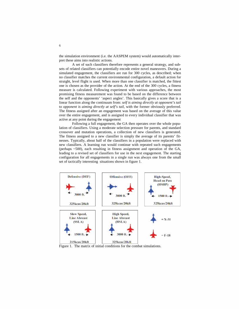
the simulation environment (i.e. the AASPEM system) would automatically inter-pret these aims into realistic actions. A set of such classifiers therefore represents a general strategy, and sub-sets of related classifiers can potentially encode entire novel maneuvers. During a simulated engagement, the classifiers are run for 300 cycles, as described; when no classifier matches the current environmental configuration, a default action for straight, level flight is used. When more than one classifier is matched, the fittest one is chosen as the provider of the action. At the end of the 300 cycles, a fitness measure is calculated. Following experiment with various approaches, the most promising fitness measurement was found to be based on the difference between the self and the opponents’ ‘aspect angles’. This basically gives a score that is a linear function along the continuum from: self is aiming directly at opponent’s tail to opponent is aiming directly at self’s tail, with the former obviously preferred. The fitness assigned after an engagement was based on the average of this value over the entire engagement, and is assigned to every individual classifier that was active at any point during the engagement Following a full engagement, the GA then operates over the whole popu-lation of classifiers. Using a moderate selection pressure for parents, and standard crossover and mutation operations, a collection of new classifiers is generated. The fitness assigned to a new classifier is simply the average of its parents’ fit-nesses. Typically, about half of the classifiers in a population were replaced with new classifiers. A learning run would continue with repeated such engagements (perhaps ~500), each resulting in fitness assignment and operation of the GA, leading to a revised set of classifiers for use in the next engagement. The starting configuration for all engagements in a single run was always one from the small set of tactically interesting situations shown in figure 1.

Figure 1. The matrix of initial conditions for the combat simulations.

7

The conditions in figure 1 were designed to generate X-31 tactics results for a balanced set of relevant situations. The early experiments described in Smith & Dike (1995) were much as just described, involving one-on-one combat, in which the LCS attempted to find novel maneuvers for the X-31, but the opponent F/A-18 aircraft used a fixed (al-though suitably reactive and challenging) set of standard maneuvers embedded in AASPEM. In short, the opponent would always attempt to execute the fastest pos-sibl turn that would leave it pointing directly at its opponent, at the same time at-tempting to match the opponent’s altitude. As reported in considerably more detail in Smith & Dike (1995), this setup led to the discovery of a wide variety of new and novel fighter maneuvers, which were evaluated in positive terms by real fighter test pilots. An example such maneuver is shown in figure 2.

Figure 2. A example of a novel maneuver evolved by the learning classifier sys-tem under the HSHP starting condition (see figure 1). The aircraft on the left is following a fixed, but reactive strategy; the aircraft on the right is following a strategy evolved by the LCS, which in turn is a new variation on the Herbst ma-neuver. The strategy discovered by the LCS in figure 2 involves pitching upwards sharply, stalling, tipping over, and then engaging the opponent with a favourable relative position. This turns out to be a variation on the ‘Herbst maneuver’ mentioned ear-

8

lier – in fact it was common for the LCS to rediscover exising maneuvers, as well as discover novel variations.

In later work (Smith et al, 2000), both opponents were controlled by a separate LCS. As Smith et al (2002) describe, in this scenario, reminiscent of the continuous iterated prisoners’ dilemma (IPD), the resulting dynamic system has four potential attractors, the most attractive of which is an ‘arms race’ dynamic, in which each pilot continuously improves his strategies. Smith et al (2000) explored various setups and indeed found that an arms race effect reliably occurs under some conditions.

Findings and Impact

Smith & Dike (1995) and Smith et al (2000) contain and discuss several more ex-amples of discovered maneuvers, including some revealing expositions of arms races that develop under the conditions of two LCSs in combat with each other. One clear result of this (still ongoing) work is the real impact it has had on its in-dustrial collaborators. In general, the aerodynamics of a new aircraft can be under-stood before the first prototype is flown; but, the complexities of piloting and combat, and consequently any real knowledge about the potential combat per-formance with skilled pilots, are much more difficult to predict. Discovering suc-cessful combat maneuvers in the way described has many advantages – in particu-lar, without the cost of test pilot time or prototype construction, LCS experiments generate rich sources of information on combat advantages (or disadvantages) that can be fed back to designers, pilots and customers. The system described briefly here, and more fully in Smith et al (2000; 2002), and Smith & Dike (1995), has re-sulted in several novel strategies that have been approved by test fighter pilots, and continue to provide useful results in a highly complex, real-world domain.

2.2 Developing an Expert Checkers Player

Our next example comes from the area of ‘computational intelligence’. The term “computational intelligence” has come to be associated largely with the major fruits of nature-inspired computing, particularly evolutionary, neural and fuzzy techniques. This is not be confused with the older, more well-established term “Artificial Intelligence”, which stands for the much wider enterprise of, by what-ever means, designing algorithms and systems that perform functions that can be called “intelligent”. Artificial intelligence (AI) includes classic areas and tech-niques such as expert systems, heuristic tree search, machine vision, natural lan-guage processing, planning, and so forth, as well as the growing range of nature-

9

inspired techniques. AI is concerned with everything from full-scale intelligent systems, through to the details of appropriate heuristics for edge detection in im-ages from a narrow domain.

Basically, almost any activity, other than those that are ‘‘easy” for computers to handle with standard techniques, can be labeled with the adjective “intelligent”. However, via natural computing, achievements have been made that will seem genuinely surprising to many people. It is no great surprise, for example, that computers can design, more successfully than humans, effective production schedules for factories with thousands of jobs per day. However it perhaps is sur-prising that we can produce software that plays checkers at the level of an expert, without encoding any expert knowledge of the game.

Blondie24

During 1999, on an internet gaming site called “The Zone”, an online checkers player with the screen name Blondie24 regularly played against a pool of 165 hu-man opponents, and achieved a rating of 2048, placing it well into the top half a percent of checkers players using that site. Blondie24 learned to play well at checkers, as did all of the good human players using that site (or otherwise). How-ever, “she” was (and still is) a computer program.

In common with many successful artificial intelligence game playing pro-grams, Blondie24 (Chellapilla & Fogel, 1999; 1999b; 2001; Fogel, 2002) incor-porates a minimax algorithm (Russell & Norvig, 2003) to traverse the game tree induced by the available moves from the current position. However, individual nodes in the tree are evaluated by an artificial neural network (ANN). The input to this ANN is a specialised representation of the current state of the game, and the output is a single value that is then used by the minimax algorithm. So far so clear – we can perhaps imagine that a well trained or well-designed ANN could be ca-pable of returning values in this context that would translate to competent check-ers playing. But how can we design, or train, such an ANN? In Blondie’s case, training was accomplished by using an evolutionary algorithm. A population of such ANNs played against each other, accumulating points over many games. The result of a game between two such ANNs comes down to a single value (per ANN) – either 1 (win), 0 (draw), or −2 (lose) – and the overarching evolutionary algorithm operates by regarding the fitness of an ANN as its total score after a number of games. In each ‘generation’ of this evolutionary algorithm, the ANNs with the lowest scores are eliminated, and new ones are generated by making mu-tant copies of the better performers, and so it continues.

For several reasons, Blondie24’s design and its success are both surprising and significant. Its prowess at checkers does not rely on tuition by human experts. In-stead, it emerges from the evolutionary algorithm process, guided only by the bare, raw total of points earned after playing several games. If an individual had a fitness of 6, for example, it was considered better (and hence had more chance for

10

selection as a parent) than an individual with fitness 4. However this takes no ac-count of the distribution of wins, losses and draws. The individual with fitness 6 may have won 6 games and drawn 4, while the individual with fitness 4 may have won 8 games and lost 2.

Guided only by this summary measure of performance, an evolutionary algo-rithm was able to traverse the space of checkers-playing-ANNs (or, more cor-rectly, ANNs for evaluating game positions in the context of minimax search) and emerge with expert-level players. It is worth covering in more detail the approach taken to generate Blondie24, which we do next, following the treatment provided in Chellapilla & Fogel (2001).

Checkers: the game

Checkers, known in some countries as ‘draughts’, involves an eight-by-eight board with squares of alternating colors, equivalent to a chessboard. Each player has 12 identical pieces, and the initial game position is as detailed in Figure 3.

Figure 3. The initial position in a game of checkers. The White player moves up-wards, and the Black player moves downwards.

When it is a player’s turn to move, the allowed moves are: an individual piece can move diagonally forward by one square; or an individual may jump over an oppo-nent’s checker into an empty square. Such a “jump” is only allowed if it takes two diagonal steps in the same direction, the first such step is occupied by an oppo-nent’s piece, and the second step is currently empty. After a jump, the opponent’s piece is removed from play.

If one or more jump moves are available, then it is mandatory for the player to make such a move. If an opponent manages to find itself in the final row (from

11

their side’s viewpoint), it becomes a “king” piece. It is then able to move either forward or backward, but otherwise follow the same rules. The object of the game is to reach a position in which your opponent has no possible moves – a common way in which this happens is for the opponent’s pieces to all have been removed.

Representing the board and evaluating moves

Chellapilla and Fogel (2001) used a straightforward and sensible approach to en-coding a board position. The current state of the game is simply represented by a vector of 32 numbers, one for each board position. The numbers in a position are either -K, -1, 0, 1, or K, where K represents a value assigned to a king. From the viewpoint of a given player, a 1 or a K at a given board position represent, respec-tively, either a standard piece or a king at that position, while the negative values are used to represent the opponent’s pieces, and zero indicates an empty position. In Chellapilla and Fogel’s work, K was not preset. Rather than bias the process towards giving a king any particular relative value over an ordinary piece, the value of K was itself subject to evolution.

When a move is to be made, Blondie24 operates by evaluating, in turn, each of its possible moves. Any such move leads to a future board position, and this future board position is evaluated by the ANN. The input to the ANN is therefore this 32-dimensional vector. As is well known from ANN theory, any reasonable ANN architecture (in terms of the number of hidden layers and the numbers of nodes in each layer) might suffice in being capable of then performing the appropriate mapping from input vector to appropriate, useful output. The difficulty, as ever, is in choosing an appropriate training regime, that promotes learning of suitable fea-tures and components of the problem state that are useful guides towards a proper evaluation. After initial experiments with a more straightforward neural network architecture (which did not encapsulate the spatial information that human players take for granted), Chellapilla and Fogel’s designed the architecture of the ANN in a way that highlighted potentially appropriate features. This was done as follows.

Each 3x3 block on the board was represented by its own unit in the first hidden layer. That is, given any specific 3x3 block, one of the units in the first hidden layer received incoming connections from that specific set of 9 inputs from the in-put layer (from the 9 parts of the vector corresponding to the component positions of that 3x3 block), and had no incoming connections from any of the other units. In this way, a specific signal emerging from this unit, for later processing in sub-sequent layers, summarises the state of play in that specific 3x3 block. The first hidden layer contained such a unit for each of the 36 different 3x3 blocks on the board. In just the same way, each 4x4 block, 5x5 block, 6x6 block, 7x7 block, and 8x8 block (of which there was of course just one) was represented in the first hid-den layer by its own unit. This resulted in a set of 91 units which comprised the first hidden layer.

12

Figure 4. The architecture of the Blondie24 artificial neural network, The complete picture of the ANN’s architecture is given in Figure 4. Between

the input layer, which simply carries 32 units, one per board position, and the first hidden layer, the connections are arranged according to the specific feature en-coded by each of the units in hidden layer 1. Between the pairs of layers, the con-nections are all complete – e.g. each unit in hidden layer 1 has a feedforward con-nection to each unit in hidden layer 2, and similar for hidden layers 2 and 3, while every unit in hidden layer 3 is connected to the single output unit. The output unit receives an additional input, which is the sum of the 32 board positions.

In total, including bias weights, there are 5046 connections in this network, each of which is a real-valued weight subject to the evolution process. In addition, every hidden layer unit has a bias input, which means an additional weight to be evolved. Each unit in the hidden layers operates in the standard way, common in most ANN applications, by calculating the weighted sum of its inputs and apply-ing the hyperbolic tanget function, resulting in an output signal strictly between -1 and 1. From the perspective of the ANN ‘player’, this ultimate scalar value is di-rectly used as an estimate of the value of this board position. The closer to 1, the better for the ANN. However, where the board position was actually a win for the ANN, the value was taken to be precisely 1, and if it was a win for the opponent the value was taken to be -1.

Full intercon-nection

. . .

32 inputs

91 feature units in hidden layer 1

. . .

Connections wired accord-ing to compo-nents of fea-tures in hidden layer 1

40 units in hidden layer 2

. . .

10 units in hidden layer 3

Full inter connection

Full inter connection plus one extra input: sum of the 32 board positions.

Single output unit

13

Evolving Checkers Players

The process begins with a population of 15 such ANNs, which are initialized ran-domly. Every connection weight and bias value is given a value chosen uniformly at random from the interval [-0.2, 0.2], and with K set initially at 2.0. In common with the practice of evolutionary programming and evolution strategies, each indi-vidual in the population also contained a vector of step size parameters. For every connection weight, and every corresponding bias unit, there was also a step-size parameter governing the range of mutations that would be applied to that parame-ter. That is, when a weight or bias parameter was mutated, this was done by add-ing a Gaussian perturbation whose mean was 0 and whose variance was provided by the associated step size parameter in the chromosome. The step-sizes were ini-tially all set at 0.05, and then subject to evolution along with the other parameters.

Whenever an ANN was selected as a parent, its offspring was generated as fol-lows: first, each of the step size parameters was mutated, by multiplying it with a random number from a specific exponential distribution, and every weight and bias parameter was mutated by adding a Gaussian perturbation whose step size was the associated step size parameter, as indicated. Finally, recall that each indi-vidual also carries its own value for K, which is also subject to evolution. This was mutated by adding a perturbation chosen uniformly at random from the set {–0.1, 0, 0.1}, but was protected from moving below 1 or above 3.

During the evolution process, Each ANN played one game each against five opponents, selected uniformly from the population. With the scoring for individual games as indicated, the ANN would therefore accumulate a score over these five games ranging from –10,(all losses) to 5 (all wins). A game was declared as a draw (zero points) if it lasted for 100 moves. Essentially, in each generation each ANN took part in around 10 games, and the top 15 (in terms of points received) became parents for the next generation. Each individual game was played using a minimax alpha-beta search set to 4-ply (with extended ply in a number of special cases). After 840 generations in which evolving ANNs played against each other, the best resulting ANN was then harvested and recruited to play against human opponents on the internet gaming site “The Zone”. In the next subsection, we summarise the surprising and remarkable resulting performance of this ANN.

Humans vs Evolved ANNs Over a two-month period, the evolved ANN, eventually named “Blondie24” (which was successful in attracting opponents) played 165 games against human opponents at “The Zone”, although opponents were not aware they were playing against a computer program. In these games, the ANN used an 8-ply search, and

14

faced a variety of opponents. The ANN’s performance placed it at better than 99.6% of all the (rated) players using the site. On one occasion, the ANN beat an expert-level player (with a rating of 2173, just below the master level of 2200) who was ranked 98th of over 80,000 registered players. Chellapilla & Fogel (2001) performed some comprehensive control ex-periments, which showed that the evolved ANN operated with a clear advantage over a system that simply used the piece differential as the basis for choosing moves in an 8-play approach. In particular, they compared the ANN with a piece-differential based player, on the basis of using equal CPU time in their lookahead search at each move; this disadvantages the ANN, since it has over 5,000 weight parameters involved in its heuristic calculation, so the piece-differential player can look further ahead in the time available. These experiments showed conclusively that the evolved ANN was a significantly better player in both equal-ply and equal CPU-time conditions. The achievement of Blondie24 is remarkable from many viewpoints: par-ticularly the essential simplicity of its approach, the fact that the search landscape for the evolutionary algorithm was so huge, and the fact that fitness assessment was a relatively coarse measure of a network’s performance. A straightforward as-sessment of Blondie24’s ‘message’ to us is that it exemplifies the flexibility and potential of evolutionary search, even when this is recruited to search a coarse-grained 10,000-dimensional landscape (the evolution strategy that was employed optimised both a weight and a step-size parameter for each connection). Achieving expert level performance (over 2,000 points) is considerably superior to most hu-mans. Perhaps not surprisingly, this is also certainly superior to a simpler (but seminal) approach in this area by Samuel (1959), which attempted to derive, by an iterative learning process, a polynomial board rating function. Chellapilla and Fogel (2001) note that this was considered to rate below 1600 in the opinion of the American Checkers Federation Games Editor.

The world champion checkers program, Chinook (Schaeffer et al, 1996), is rated at over 2800, over 100 points above its closest human competitors (Schaeffer, 1996). In fact it is now known that Chinook can never be defeated in `go-as-you-please’ checkers, in which there are no restrictions on the initial moves. The chief difference between Blondie24 and Chinook is the amount of built-in specialised knowledge. In Chinook, the level of such knowledge is very substantial indeed; in Blondie24 it is virtually none. Along with many other ele-ments informed by careful expert knowledge and tuning, Chinook incorporates a database of games from previous grand masters and a complete endgame database for all cases that start from ten pieces or fewer. Blondie24 and Chinook represent entirely different artifical intelligence approaches to designining a game-playing program. It is not difficult to argue that the approach taken by Blondie24 is the more interesting and impactful – from no prior knowledge, other than a built-in awareness of the rules of the game, an expert level player emerged from the evolu-tionary process, providing a very tough, usually unsurmountable challenge to all but a very small percentage of human players.

Finally, since the checkers research, Chellapilla & Fogel’s approach was extended to address chess, by combining the co-evolutionary spatial neural net-

15

work approach with domain-specific knowledge (Fogel et al, 2004; 2006). The re-sult was an evolved chess player that earned wins over Fritz 8, which was the 5th best computer program in the world at that time.

2.3 Discovering Financial Trading Rules

Financial markets are complex and ever-changing environments in which groups of individuals, companies and other investors are always competing for profit. There are many opportunities in this area for machine learning and optimization methods, and consequently a variety of natural computation approaches, to be ex-ploited, and a chapter in this volume is indeed devoted to this topic. In this section, we focus on one specific thread of research in this area – which has a simply grasped approach and a straightforward task to solve. This is the use of genetic programming to discover new and valuable rules for financial trading.

It is now common to see applications of evolutionary computation applied to the financial markets (Brabazon & O’Neil, 2005; this volume). Genetic Program-ming (GP) (Koza, 1992; Angeline, 1996; Banzhaf et al, 1998) is particularly prominent in terms of the degree to which it has recently been applied in finance (Chen & Yeh, 1996; Fyfe et al, 1999; Allen & Karjaleinen, 1999; Marney et al, 2001; Chen, 2002; Cheng & Khai, 2002; Farnsworth et al, 2004; Potvin et al, 2004). In this section we focus on the specific area in finance known as technical analysis (Pring, 1980; Ruggiero, 1997; Murphy, 1999; Lo et al, 2000). Technical analysis is a set of techniques that forecast the future direction of stock prices via the study of historical data. Many different methods and tools are used, all of which rely on the principle that price patterns and trends exist in markets, and that these can be identified and exploited.

Common tools in technical analysis include indicators such as moving aver-ages (the mean value of the price for a given stock or index over a given recent time period), relative strength indicators (a function of the ratio of recent upward movements to recent downward movements). There have been a number of at-tempts to use GP in technical analysis for learning technical trading rules, and a typical strategy is for such a GP-produced rule to be a combination of technical indicator ‘primitives’ with other mathematical operations. Such a rule is often called a ‘signal’. E.g. GP may be employed to find both a good buy signal and a good sell signal – that is, one rule which, if its output is above 0, indicates that it is a good time to buy, and a different rule indicating when it is a good time to sell.

Early attempts to use GP in technical trading analysis were by Chen and Yeh (1996) and Allen and Karjalainen (1999). However, although GP could produce profitable rules for the stock exchange markets, their performance did not show any benefit when compared to the standard buy-and-hold approach. ‘Buy-and-hold’ simply means, for a given period, buying the stock at the beginning of the

16

period, and selling at the end – hence, always a good idea in a market that gener-ally moves up during the period.

More recent applications of GP in this context have been more encouraging (Marney et al, 2000; 2001; Neely, 2001). We will look in particular at Becker & Seshadri’s work (2003a; 2003b; 2003c) which found GP-evolved technical trading rules that outperformed buy-and-hold (at least if dividends are excluded from stock returns). In turm, their approach was founded in Allen & Karjeleinen (1999), with various modifications. After giving some detail of the overall approach, we summarise from further experiments from Lohpetch & Corne (2009; 2010) that probed certain boundaries of the technique and examined its robustness.

Becker & Seshadri’s approach to evolving trading rules

Becker & Seshadri (2003a; 2003b; 2003c), based on Allen & Karjeleinen (1999) used a fairly standard GP approach and found rules that significantly outperformed buy-and-hold on average over a 12-year test period of trading with the Standard & Poors (S&P500) index. Their GP’s function set contained the standard arithmetic, Boolean and relational operators, and the terminal set included some basic techni-cal indicators. An example of a specific rule found by their method is in Figure 5.

Figure 5. Example of a trading rule found by Becke & Seshadri’s GP approach.

The rule in figure 5 has the following basic interpretation “ the 3-month mov-

ing average (MA-3) is less than the lower trend line (t) and the 2-month moving average (MA-2) is less than the 10-month moving average (MA-10) and the lower trend line (t) is greater than the second previous 3-month moving average maxima (MX-2)” . This signals trading behaviour in the following way: If the trader is cur-rently out of the market (no stocks invested in the S&P500), and the rule evaluates to true, then buy; if the trader is currently in the market, and the rule becomes

17

false, then sell.. This procedure assumes a fixed amount to invest (e.g. $1,000) whenever there is a buy signal.

In the remainder of this subsection we explain the approach in more detail, and try to emphasise the key points that are necessary to replicate similar perform-ance. In passing we note the main ways in which Becker & Seshadri modified the original approach of Allen & Karjeleinen. These were: monthly trading decisions rather than daily trading; a reduced function set in the GP approach; a larger ter-minal set in the GP approach (with more technical indicators); the use of a com-plexity-penalising element to avoid over-fitting; and finally, modifying fitness function to consider the number of periods with well-performing returns, rather than just the total return over the test period. In combination, these methods en-abled Becker & Seshadri to find rules that outperformed buy and hold for the pe-riod they tested, when trading on the S&P500 index. It is an open question as to which modifications were most important to this achievement, however Lohpetch & Corne (2010) begins to answer that question, as we will see, by showing (as is intuitiely the case) that it is increasingly easier to find good rules as we change the trading interval from daily to weekly, and then to monthly.

In the following, we exclusively use S&P500 data (as did Allen & Kar-jeleinen (1999) and Becker & Seshadri (2003a; b; c); so, our ‘portfolio’ is the fixed set of 500 stocks in the S&P500 index, which, aggregate to provide daily price indicators.

Function and Terminal Sets used by Becker & Seshadri

In Becker & Seshadri’s GP approach, the function set comprises simply the Boo-lean operators and, or and not, and the relational operators > and <. The terminal set comprises the following, in which ‘period’ was always month in Becker & Se-shadri’s work, but later we discuss Lohpetch & Corne (2010) in which it could be day, week or month in different experiments.

• opening, closing, high and low prices for the current period; • 2,3,5 and 10-period moving averages; • Rate of change indicator: 3-period and 12-period; • Price Resistance indicators: the two previous 3-period moving average

minima, and the two previous 3-period moving average maxima; • Trend Line Indicators: a lower resistance line based on the slope of the

two previous minima; an upper resistance line based on the slope of the two previous maxima.

The n-period moving average at period m is the mean of the closing prices of the n previous months (included m). The n-period rate of change indicator measured at period m is: (c(m) −c(m−(n−1))×100)/c(m−(n−1)), where c(x) indicates the closing price for period x. Previous maxima MX1 and MX2 are obtained by considering the 3-period moving averages at each point in the previous 12 periods. Of the two highest values, that closest in time to the current period is MX1, and the other is

18

MX2. the two previous minima are similarly defined. Finally, to identify trend line indicators, the two previous maxima are used to define a line in the obvious way, and the extrapolation of that line from the current period becomes the upper trend line indicator; the lower trend line indicator is defined similarly, using the two pre-vious minima.

Becker & Seshadri’s Fitness Function The fitness function has three main elements. First is the so-called ‘excess return’, indicating how much would have been earned by using the trading rule, in excess of the return that would have been obtained from a buy-and-hold strategy. The other elements of the fitness function were introduced by Becker and Seshadri to avoid overfitting. These were: a factor that promoted fitness for trading rules that were less complex (e.g., with reference to figure 5, a less complex rule is one in which the tree has smaller depth); and, a factor that considered ‘performance con-sistency’ (PC), favouring rules that generally were used often, each time providing a good return, rather than rules that were very fortunate in only brief periods.

In more detail, the excess return is simply bhrrE −= , where r is the return on

an investment of $1,000, and rbh is the corresponding return that would have been achieved using a buy and hold strategy. To calculate r, Allen & Karjeleinen (1999) and Becker & Seshadri (2003a; b; c) used:

)1

1ln()()()(

11 c

cntItrtIrr

T

tsf

T

tbt +

−++= ∑∑==

in which: 1loglog −−= ttt PPr , indicating the continuously compounded re-

turn, where Pt is the price at time t. The term Ib(t) is the buy signal, either 1 (the rule indicates buy at time t) or 0. The sell signal, Is(t), is analogously defined. So, first component gives the return on investment from the times when the investor is in the market, and the second component, rf(t) indicates the risk-free return which would otherwise be available, which is taken for any particular day t from pub-lished US Treasury bill data (these data are available from http://research.stlouisfed.org/fred/data/irates/tb3ms). The second component there-fore represents time out of the market, in which it is assumed that the investor’s funds are earning a standard risk-free interest. Finally, the third component is a cor-rection for transaction costs, estimating the compounded loss from the expenditure on transactions; a single transaction is assumed to cost 0.25% of the traded volum – e.g. $2.50 for a transaction of volume $1,000. The number of transactions actioned during the period by the rule is n.

The second main part of the fitness function, rbh, is calculated as:

)11

ln(c

crr tbh +

−+=∑

in which rt is as indicated above. This calculates the return over the period from risk-free investment in US Treasury bills, involving a single buy transaction.

19

Becker & Seshadri’s complexity-penalising adjustment works as follows: Given a rule that has depth depth and fitness value (excess return) f, the adjusted fitness becomes 5f/max(5,depth). This involves the constant 5 as a relatively arbi-trary desired maimal depth, and in the trading rule evolution context, there has been little paramertic investiagtion around this value so far. The other of Becker & Se-shadri’s modification to the excess return fitness function, Performance Consis-tency (PC) works as follows. The excess return E is calculated for each successive group of K windows of a certain length covering the entire test period.

The value returned is simply the number of these periods for which E was greater than both the corresponding buy and hold return (from investing in the in-dex over that period) and the risk-free return during that period. For example, if the rule is evaluated over a 5 year test period, the PC version of the fitness function might use 12-month windows. Clearly there are five such windows in the test pe-riod, and the fitness value returned will simply be an integer between 0 (the rule did not outperform buy and gold and risk-free investment in any of the five windows) and 5 (the rule was more successful than both buy-and-hold and risk-free return in all of the windows).

At last, the above background enables us to state the fitness function used (with minor variations in each case) in Becker & Seshadri (2003a; b; c) and Lohpetch & Corne (2009; 2010). The fitness of a GP tree of depth d in these studies was the performance-consistency based fitness (i.e. a number from 0 to X, where there were X windows covering the test data period), adjusted to penalise undue complexity in by 5f/max(5,d), in which f is the number of the X windows in which both the corre-sponding buy and hold return and the risk-free return were outperformed by the rule.

Some illustrative results We report here some results that show how this approach performs on various win-dows of time when trading with the S&P500 index. The results we show are some of those from Lohpetch & Corne (2010), and the subset of those that were obtained under the same test conditions as used by Becker & Seshadri (i.e. monthly trading for a specific training and test window) are quite indicative of Becker & Seshadri’s own results. However, it is worth first discussing some fruther details of the way that the genetic programming method was set up for the experiments.

Although perhaps not always the case, it seems that the precise choice of mutation and crossover methods makes little real difference in this application; the chance of evolving effective trading rules seems clearly related to a good choice of function and terminal sets for the expression trees, as well as a wise choice of fit-ness function. Although, as we will see later, the frequency of trading is a signifi-cant factor. Meanwhile, Lohpetch & Corne (2009; 2010) used standard mutation operators, as described by Angeline (1996), namely grow, switch, shrink, and cycle mutation, and used standard subtree-swap crossover (Koza, 1992). Finally, we note that, in the experiments whose results we summarise next, the population was ini-tialized by growing trees to a maximum depth of 5, however no constraint was placed on tree size beyond the initial generation, other than the pressure towards less complex trees which is a part of the fitness function.

20

We can now show some results that indicate the performance achievable by such a GP system as described in the last section. In the experiments summa-rised here, from Lohpetch & Corne (2009; 2010), a population size of 500 was used, and other relatively standard GP settings, with a run continued for 50 genera-tions. Here we show results for each of daily, weekly and monthly trading, and we find that outperfomance of buy-and-hold can indeed be achieved even for daily trading, but as we move from monthly to daily trading the performance of evolved rules becomes increasingly dependent on prevailing market conditions. The data used is the S&P500 index from 1960 onwards. In Becker & Seshadri’s demonstra-tion of outperforming buy-and-hold, only monthly trading was used, and their re-sults arise from training the rules over the1960—1991, and evaluating them on a test period spanning 1992—2003. This corresponds to “MonthlySplit1” in the fol-lowing, however it is clear from Lohpetch & Corne (2009) that more robust per-formance is obtained when a validation period is used. The following illustrative results therefore reflect a training/validation/test regime in which the GP training run evaluated fitness on the training period only, but the rule that achieved the best performance on a validation period was harvested, and this was the rule evaluated on the test period.

Results for four different monthly trading data splits are summarized below. The splits themselves are as follows, in which N gives the length of the validation period in years, immediately following the training period, and K gives the length of the test period in years, again immediately following the validation period.

• MonthlySplit1: 31 yrs training; N=12, K=5 • MonthlySplit2: 31 yrs training, N=8, K=8 • MonthlySplit3: 31 yrs training, N=9, K=9 • MonthlySplit4: 25 yrs training, N=12, K=12

Corresponding splits for the weekly and daily trading experiments are also su-marised here very briefly (for details see Lohpetch & Corne (2010)). Four different weekly trading and daily trading data splits were also investigated, roughly corre-sponding to the monthly data splits in terms of the number of data points in each split. E.g. WeeklySplit1 involved 366 weks trading, 158 weeks validation and 157 weeks testing. Similarly, the training periods for the daily splits were approxi-mately one year in length. The four different weekly and daily splits started at dif-ferent times spread evenly between 1960 and 1996.

Figure 6 shows the four Monthly data splits aligned against the S&P 500 index for the period 1960—2008. Note that the market movements were net posi-tive in each part of each split, indicating that outperforming buy-and-hold was in all cases a challenge.

21

Figure 6. The S&P500 index over the period 1960—2008, illustrating the four data splits for the case of monthly trading.

In Lohpetch & Corne’s experiments (2010), they also explored different lengths of window for the Performance Consistency element of the fitness function. In Becker and Seshadri’s work, the Performance Consistency approach clearly results in improved performance, however they only reported on the use of 12-month win-dows. Lohpetch & Corne experimented with different lengths for these windows for each trading situation, namely: 6, 12, 18 and 24 months periods for monthly trading; 12 and 24 weeks for weekly trading, and 12 and 24 days for daily trading.

For each trading period (monthly, weekly, daily), Lohpetch & Corne did 10 runs for each combination of data split and consistency of performance period. The outcome of the 10 runs is summarised in Tables 1—3, simply as the number of times that the result outperformed buy-and-hold.

Table 1. Summary of results for monthly trading

Data split PC Period

Trials outperforming buy-and-hold.

PC Period

Trials outperforming buy-and-hold.

Monthly Split1 6 10 out of 10 12 10 out of 10

Monthly Split2 6 9 out of 10 12 10 out of 10

Monthly Split3 6 10 out of 10 12 9 out of 10

Monthly Split4 6 10 out of 10 12 10 out of 10

Monthly Split1 18 10 out of 10 24 10 out of 10

Monthly Split2 18 8 out of 10 24 10 out of 10

Monthly Split3 18 8 out of 10 24 7 out of 10

Monthly Split4 18 10 out of 10 24 10 out of 10

1965 1970 1975 1980 1985 1990 1995 2000 2005

22

As Table 1 shows, monthly splits 1 and 4 were clearly well-disposed to good performance, but performance was also rather robust on the other monthly splits. Note that outperforming buy and hold would seem to be more likely, according to a priori intuition, when the performance of buy-and-hold in the test period is rela-tively weak, but this is not the case for Monthly splits 1 and 4 (see Figure 6). The results are quite impressive from many points of view. In many cases, ten tests out of ten showed that a simple trading rule evolved by genetic programming was able to outperform buy-and-hold in an upwardly moving market.

Table 2. Summary results for weekly trading

Data split PC Period

Trials outperforming buy-and-hold.

PC Period

Trials outperforming buy-and-hold.

Weekly Split1 12

2 out of 10 24

7 out of 10

Weekly Split2 12 10 out of 10 24 5 out of 10

Weekly Split3 12 4 out of 10 24 4 out of 10

Weekly Split4 12

10 out of 10 24

10 out of 10

Table 2 shows the results, summarized in the same way, for the case of weekly

trading, and Table 3 presents the corresponding results for the case of daily trading. These clearly show increasingly less robust results. It certainly seems that this rela-tively straightforward GP method can find robust rules for weekly trading that out-perform buy-and-hold in some circumstances (splits 2 and 4), with less reliable per-formance in other cases. However, Lohpetch & Corne (2009; 2010) were not able to discern any pattern that explains this from analyses of the data splits. Finallly, for daily trading, Table 3 shows that outperforming buy-and-hold is less likely, with strong performance in only one of the four data splits, and very poor performance in two of the data splits.

Table 3. Summary of results for daily trading

Data split PC Period

Trials outperforming buy-and-hold.

PC Period

Trials outperforming buy-and-hold.

Daily Split1 12

0 out of 10 24

0 out of 10

Daily Split2 12 0 out of 10 24 0 out of 10

Daily Split3 12 10 out of 10 24 9 out of 10

Daily Split4 12

2 out of 10 24 4 out of 10

23

A Brief Discussion

The investigation of genetic programming in financial applications, and in particu-lar the use of it to discover technical trading rules, remains an active thread of re-search in both industry and academia. In the published academic research, it was commonly found in earlier studies that rules found by genetic programming were profitable, but usually not competitive with straightforward “buy and hold” strate-gies. However, as we have seen, the situation is changing and it now seems that progress is being made in finding ways to use genetic programming to produce ef-fective and interesting rules that might be used by individual traders. There are sev-eral caveats, and of course this enterprise is only one thread of work in a wide area that also involves natural language understanding and many other areas of machine learning (for example, to spot ideal trading opportunities based on the latest online news). However this work represents another example of the way in which natural computation can help us generate strategies for complex situations which are com-petetive with those we design ourselves.

We should also note that the approach described in this section is far from the last word in the application of genetic programming to the specific area of technical trading. We have taken pains to describe a classic approach, and shown that it can indeed find robustly profitable trading rules under a range of conditions – however several more sophisticated ways to use GP in this area also exist. For example, rather than simply evolve a single rule that encapsulates both a buy and sell signal, different rules can be evolved separately for buying and selling. Also, we note that interested researchers may pick up code for evolving technical trading rules (writ-ten by Dome Lohpetch) from the following site:

http://www.macs.hw.ac.uk/~dwcorne/gptrcode/. It is also worth mentioning alternative directions which attempt to gain on

buy-and-hold by including risk metrics in the rules (or in their evaluation). Typi-cally, a risk measure such as the Sharpe ratio (Sharpe, 1996) is used to normalize the estimate of financial return, effectively downgrading the performance of rules that promote trading in volatile conditions, promoting rules more likely to be ap-plied by investors. For example, in attempting to build on work by Fyfe et al (1999), Marney et al (2000; 2001) included the use of metrics for calculating risk, although still did not outperform buy-and-hold. More recently, Marney et al (2005) used the Sharpe ratio and found that a technical trading rule that easily out-performed simple buy and hold in terms of unadjusted returns, but not in terms of risk-adjusted returns. There is clearly much work still to do until techniques exist in the research literature that can robustly outperform buy-and-hold in a way that satisfies risk-conscious traders, although the progress and effort in this direction makes it clear that this will be achieved, as well as suggesting that private and un-published research in commercial organizations has almost certainly achieved this already with appropriate use of genetic programming and similar technologies.

24

3. Examples of Natural Computing’s ‘Outreach’ elsewhere in Science and Engineering

In this section we select two areas of natural computation which have wider impli-cation for significant areas of science and technology. Mostly, an application of a natural computing technique may produce excellent results in its domain, and the impact of those results, though potentially significant, tend to remain solidly within that domain. Progress in general financial mathematics, for example, will not be revolutionised by the trading application we discussed in section 2. How-ever, sometimes an exemplar application will open up previously unconsidered possibilities in a whole subfield of science. In this section we discuss two exam-ples in which we can see such broader consequences. The first is the use of (mostly) multi-objective evolutionary computation in the area of closed-loop op-timisation, in order to optimise a range of processes and products in the biosci-ences, process industries and other areas. In this arena, evolutionary computing was never an `obvious’ technique to try, given the potential cost in time, however it’s use has time and again proven worthy, and this in turn leads directly to better and faster processes and products emerging from, for example, the use of the in-struments that have been configured via evolutionary techniques. The second exe-ple area we look at in this section is the concept of innovization, which exploits multi-objective evolutionary computation in a way that leads to generic design in-sights for mechanical engineering (and other) problems. In multi-objective prob-lems (see Deb, 2001; Corne et al, 2003) the result of solving the problem is a (usu-ally) large collection of diverse solutions, each optimal in a sense, but traversing a Pareto surface of optimal from (for example) highly reliable and high cost solu-tions to exceptionally cheap but less reliable ones. The notion of innovization is to exploit the prowess of evolutionary computing in obtaining such a diverse set, by further analysing this collection of designs to find, as it turns out, previously un-known generic design rules which seem to be true of all ‘optimal’ designs, wher-ever they sit on this Pareto surface. A well designed natural computing approach to a specific problem in mechanical engineering, for example, thereby leads to new design principles that can have much wider impact than simply solving the given problem.

3.1 Applications in Analytical Science: Closed-Loop Evolutionary Multiobjective Optimization

Knowles (2009) provides a detailed and comprehensive summary of historical ori-gins and current work in the broad area of closed-loop optimisation using evolu-tionary multiobjective algorithms. We provide a similar but more brief treatment

25

here, including a summary of two of the several interesting modern case studies covered in Knowles (2009).

As Knowles (2009) points out, the idea of using an evolution-inspired technique for producing solutions to optimization problems has been explored for around 60 years so far, starting in the 1950s. The celebrated British statistician George E.P. Box used the term ‘closed-loop’ in describing the kind of evolution experiments that were first investigated, while Ingo Rechenbrg (a pioneer in evo-lutionary computation) used the phrase ‘evolutionary experimentation’. In closed-loop evolution-inspired optimisation, the evolution process is a combination of computation and physical experiment. The evaluation of candidate design solu-tions is done in the real world by conducting physical experiments. Much of the pioneering work in evolutionary computation (by Rechenberg and his team) was of this kind. In much more recent times, the closed-loop approach has been used, commonly with much success, in evolvable hardware research (see chapter in this volume), in evolutionary robotics research, as well as in microbiology and bio-chemistry. In this section, some brief example case studies are described, to illus-trate the increasingly wide emerging impact of this technique at the evolu-tion/engineering interface.

With a focus on closed-loop evolutionary multiobjective optimization (CL-EMO) in particular, we look at two cases (i) instrument optimization in ana-lytical biochemistry; (ii) on-chip synthetic biomolecule design; these are described in greater detail in Knowles (2009) as well as further references detailed later, and along with other quite different examples. However, before these case notes, we will briefly look at the historical development and fundamental concepts in closed-loop optimization and CL-EMO.

Historic Highlights in Closed-Loop Optimization

In Berlin in the 1960s, Rechenberg, Schwefel, and Bienert conducted a series of studies in engineering and fluid dynamics, in which they tested the idea of using a process inspired by evolution to search for new and successful designs. Their work clearly demonstrated that complex design engineering problems (including: the optimal shape of a fluid-bearing pipe, and the design of a supersonic jet noz-zle) could be addressed in this way with rampant success (see Chapter 8 of Fogel (1998), as well as Rechenberg (1964; 2000). The design process itself was found to be efficient and scalable, and the results were highly effective. Rechenberg and his team were using an early example of an evolutionary algorithm, but in which only the selection and variation steps were done by a microprocessor; the rest, the evaluation of candidate designs, was done by constructing prototype designs and performing experiments to test their properties. Innovative solutions were found to all of the engineering design problems that they studied.

Pre-dating Rechenberg’s work, a similar principle was used by George Box, who introduced ‘evolutionary operation’ (EVOP) in 1957. This was also an ex-

26

perimental method of optimization, which Box (1957) envisaged being used regu-larly in factories and similar processing facilities. Box’s ‘closed-loop’ scheme in-volved some human input, and was somewhat more deterministic than the ap-proach taken in Berlin, but, just as Rechenberg’s work, was inspired by principles from natural evolution. Box’s methods were both successful and very influential (Hunter & Kittrell, 1966), remaining in use today. Meanwhile, the work of Re-chenberg’s team was the beginning of the field of evolution strategies, one of the foundation stones of the current field of evolutionary computation.

Since these early studies, however, evolutionary computation as a whole has largely been concerned with entirely in silico optimisation. The great majority of growth in this research area, as well as in industrial practice, concerns applications that involve convenient and entirely computational estimations of the fitness of computational abstractions of solutions. This is fine for a vast collection of scenar-ios, but there remains a need – in fact a quickly expanding one – for applications in which it makes sense for designs to be realised and evaluated physically throughout the simulated evolution process.

Research in evolvable hardware shows that, if the evolution processs is given direct access to a complex physical structure, designs can be evolved that use en-tirely different proinciples than would be used by human designers, often exploit-ing aspects of the physics of the structures involved that are unfamiliar to human experts, or simply too difficult to use as part of the design process. Thompson & Layzell’s work with Field Programmable Gate Arrays is exemplary of this. Meanwhile, evolutionary robotics projects have often relied upon the controllers being evolved in real time within physical robots, while they are performing real tasks in a real environment (Nolfi & Floreano, 2004; Trianni et al, 2006). The benefits of such evolution experiments, exposed to and exploiting the true physics of the designs being evolved, are not just confined to evolutionary robotics, e.g. Davies et al (2000), Evans et al (2001).

Later, we describe three further and recent uses of closed-loop evolutionary op-timization, from recent work in which the third author (JDK) has been involved. Each is a scenario where direct experimental evaluation of solutions is either the only option or is clearly preferable to simulation. Also they each involve multiob-jective evolution, a notable advance of the last twenty years (Fonseca & Fleming, 1995; Coello, 2000; 2006; Deb, 2001; Corne et al, 2003) which was not available to Box or Rechenberg. One of the several benefits of a multi-objective approach in these scenarios is that the different design objectives may simply be stated, with-out any need to define normalizations, weights or priorities that mangle them into a single scalar (and usually misleading) measure of quality.

At this point, it is worth noting that there is widespread use of certain statistical methods in industry, for the types of problems that we are considering in the ‘closed loop’ setting. The techniques employed are referred to as design of ex-periments (DoE) approaches, or sometimes experimental design (ED) based ap-proaches (Fisher, 1971; Chernoff, 1972; Myers & Montgomery, 1995; Box et al, 2005). Such methods emphasise rational reasoning from all the information ob-tained so far, as opposed to more randomized exploration. Standard DoE is typi-

27

cally used for probing low-dimensional parameter spaces using few experiments, while evolutionary algorithms are typically used for optimization in high-dimensional spaces, using many evaluations, and optimize many different types of structure, including permutations, graphs, networks, and so on. However, there is an increasingly disappearing divide between the two types of approach, especially since the advent of sequential DoE, which incorpates aspects of evolutionary computing. The closed-loop optimization scenarios considered in this section lie between these niches, and benefit from aspects of both approaches.

Fundamentals of Closed-Loop Evolutionary Multiobjective Optimiza-tion

In closed-loop EMO, candidate solutions to a problem are generated by an algo-rithm in computer simulation, but their evaluation is achieved by physical experi-ment. Evaluations are fed back to the algorithm and its generation of subsequent solutions is a function of these. Thus the process has the form of a closed loop, be-ing at least partially sequential. Closed-loop problems can be defined generally as multiobjective optimization problems in which, essentially, we need to find some ideal solution vector x, which simultaneously minimizes each of a collection of k objective functions f1(x), f1(x), … fk(x). Typically, a single physical experiment g(x) yields the k measurements f1(x), f1(x), … fk(x). That is, the k objectives are k different measurements that are made as the result of a single experiment, all of which we need to optimize in some way. Typically, at least some of the objectives will be in conflict (Brockhoff & Zitzler, 2006), and no single solution is a mini-mizer of all functions. Rather, the improvement of one objective is only possible by sacrificing, or trading off, quality in some other objective. The solutions corre-sponding to optimal values of the k objectives are known as the Pareto set, and when plotted in objective space, form the Pareto front (see Figure 7).

28

Figure 7: An illustration of a Pareto front for a typical optimization problem with two ob-jectives,both of which have to be minimized. Eacg of the solutions on the Pareto Front (PF) are optimal in the Pareto tradeoff sense. E.g. for any solution on the PF, no silution exists which is improved in one objective without being degraded on another objective. Often, some solutions on PFs are ‘unsupported’ – these are valid optimal solutions in the Pareto tradeoff sense, but for any linear combination of the objectives that might be used in a sin-gle-objective simplification of the problem, they would not be optimal.

Since solving such a vector optimization problem usually leads to a set of solu-

tions, rather than a single one, there is, in most practical applications, a need for decision making to select one solution from this set. This aspect of multi-objective optimization is important and well-studied (Fonseca & Fleming, 1998; Miettenen, 1999; Branke & Deb, 2005, and we will not cover the various alternative ap-proaches here. Suffice to say that in the experiences detailed later, the EMO algo-rithms were designed to find whole Pareto fronts, with the expectation that a hu-man decision maker would make the final decision using the information incorporated in the output Pareto front.

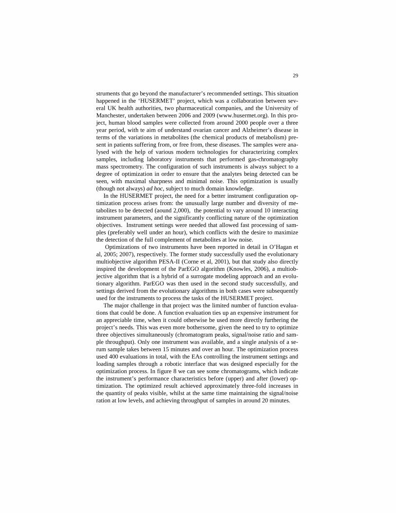
Example 1: Instrument Optimization in BioAnalytical Chemistry Modern biotechnology and bioanalytics often involves large-scale experiments which impose heavy demands on sophisticated laboratory instruments. To achieve timely throughput, these experiments often necessitate using configurations of in-

Objective 1

Objective 2 Solutions on the Pareto front

Unsupported solutions (in a concave region)

Dominated solutions (not on the Front)

29

struments that go beyond the manufacturer’s recommended settings. This situation happened in the ‘HUSERMET’ project, which was a collaboration between sev-eral UK health authorities, two pharmaceutical companies, and the University of Manchester, undertaken between 2006 and 2009 (www.husermet.org). In this pro-ject, human blood samples were collected from around 2000 people over a three year period, with te aim of understand ovarian cancer and Alzheimer’s disease in terms of the variations in metabolites (the chemical products of metabolism) pre-sent in patients suffering from, or free from, these diseases. The samples were ana-lysed with the help of various modern technologies for characterizing complex samples, including laboratory instruments that performed gas-chromatography mass spectrometry. The configuration of such instruments is always subject to a degree of optimization in order to ensure that the analytes being detected can be seen, with maximal sharpness and minimal noise. This optimization is usually (though not always) ad hoc, subject to much domain knowledge.

In the HUSERMET project, the need for a better instrument configuration op-timization process arises from: the unusually large number and diversity of me-tabolites to be detected (aound 2,000), the potential to vary around 10 interacting instrument parameters, and the significantly conflicting nature of the optimization objectives. Instrument settings were needed that allowed fast processing of sam-ples (preferably well under an hour), which conflicts with the desire to maximize the detection of the full complement of metabolites at low noise.

Optimizations of two instruments have been reported in detail in O’Hagan et al, 2005; 2007), respectively. The former study successfully used the evolutionary multiobjective algorithm PESA-II (Corne et al, 2001), but that study also directly inspired the development of the ParEGO algorithm (Knowles, 2006), a multiob-jective algorithm that is a hybrid of a surrogate modeling approach and an evolu-tionary algorithm. ParEGO was then used in the second study successfully, and settings derived from the evolutionary algorithms in both cases were subsequently used for the instruments to process the tasks of the HUSERMET project.

The major challenge in that project was the limited number of function evalua-tions that could be done. A function evaluation ties up an expensive instrument for an appreciable time, when it could otherwise be used more directly furthering the project’s needs. This was even more bothersome, given the need to try to optimize three objectives simultaneously (chromatogram peaks, signal/noise ratio and sam-ple throughput). Only one instrument was available, and a single analysis of a se-rum sample takes between 15 minutes and over an hour. The optimization process used 400 evaluations in total, with the EAs controlling the instrument settings and loading samples through a robotic interface that was designed especially for the optimization process. In figure 8 we can see some chromatograms, which indicate the instrument’s performance characteristics before (upper) and after (lower) op-timization. The optimized result achieved approximately three-fold increases in the quantity of peaks visible, whilst at the same time maintaining the signal/noise ration at low levels, and achieving throughput of samples in around 20 minutes.

30

Figure 8: Chromatograms indicating detection performance of the instrument op-timized in the HUSERMET project. (a) from the initial generation of search; (b) towards the end of the search process. In (b), both the number of peaks and the range of retention times over which peaks are detected have improved, while maintaining noise at low levels.

31

Example 2: Evolving Real DNA on Custom Microarrays

Another example covered in more detail in Knowles (2009) concerns the design of pharmacologically-active, highly-targeted macromolecules. This is a significant goal in modern medicine, especially in the context of ab initio design, where we seek a molecule with specific properties and activity, but have little or nothing to go on (in the sense of existing molecules with similar properties). In recent re-search, novel microarray-based technology has been used in the automation of such ab initio molecule design. Experimental biotecthnology platforms are now available which can synthesise, and then experimentally test in a variety of ways, any specifed DNA sequence. Being able to synthesize any given sequence, and subject it various tests, means there is far less need for computational models which, in the current state of the art, are far from good enough (or fast enough) to support such a process.

The microarray used in the work described next (and more fully in Knowles (2009) and references therein) is the so-called CustomArray technology, available from Combimatrix Corp, which can be used to synthesise up to 90,000 specific bespoke DNA sequences of up to 40 bases lomg in a single experiment. Once the sequences have been synthesized. they can be tested for a variety of properties, but usually the main property of interest is the ability to bind to a particular target molecule. In the testing (or assay) process for binding ability, the chip holding the sequences is ‘washed’ with a solution containing the target molecule, and some form of fluorescent tagging is used so that binding can be observed; further auto-mated processes can then estimate the strength of binding.

Short strands of DNA (or RNA), which bind strongly to specific targets are called aptamers, and hundreds of these have been developed for a wide variety of applications. Before the recent microarray-based work at Manchester (which is what we are discussing here, with full details in Knight et al (2008)), new aptam-ers were almost always discovered by a method called SELEX (Tuerk & Gold, 1990), or in vivo selection, in which the DNA strands are evolved in a test tube by repeated rounds of high-pressure selection and random mutation. As indicated, however, in the microarray approach we know precisely the sequence information for every sequence tested, and can even exactly specify mutations or other varia-tions to perform. This is not the case in SELEX, and one of the many benefits for the microarray approach is that it allows extremely richer possibilities for borrow-ing and exploiting algorithms from evolutionary computation, machine learning and statistics.

Knight et al (2008) reports the first use of an evolutionary algorithm to produce a DNA aptamer on the B3 Combimatrix platform. This happened after ten genera-tions of evolution, eventually discovering several 30-base long strands that bound very strongly to the target molecule, allophycocyanin. The work in Knight et al (2008) used a DNA chip that could hold 6,000 strands. With 90,000 strands on a

32

chip now possible in more modern technology, one main challenge (from the op-timization perspective) is to determine the best way to exploit such massive popu-lation sizes. Wedge et al (2009) have recently explored such questions in in silico simulations using contrived search landscapes, as well as real trials on the DNA landscape, revealing, among other findings, that higher than standard mutation rates consistently outperformed a range of other setups. This echoes findings in Corne et al (2003b), which also explored large population sizes and contrived in silico landscapes, partly to inform the (as then) emerging field of closed loop pro-tein evolution.

Some Concluding Notes on CL-EMO For the examples described above, and several more in which CL-EMO has been used, building accurate computational models that could usefully replace real ex-periments is practically infeasible. The closed-loop alternative offers a more effi-cient and effective way towards the discovery of innovative solutions, easily mak-ing up for the time and expense of tying down the physical kit for the experimental period. One question often worth asking, however, is whether we need to automate the optimization process at all in such scenarios. There is a proc-essing step in which a computational process (here, e.g. an evolutionary multiob-jective optimization algorithm) considers the latest experimental evaluation re-sults, and outputs sample designs for the next sequence of physical evaluations – but this operation could easily be done instead by a domain expert. On the other hand, though, there are several objections to such human involvement: even ex-perts can over-interpret results that are affected by noise or similar factors; simi-larly, humans are very prone to reason on the basis of simple models, ignoring in-teractions between parameters. Meanwhile there is always a very real danger of experts preferring solutions that are (or are close to) known designs.

Problems where accurate computer modeling is infeasible, and for which closed-loop optimization is the efficient solution, are really quite common. For the moment, the main focus of the third author is on problems in modern biology, where there is a growing take-up of multiobjective optimization. Meanwhile, many other substantial areas are able to benefit greatly from CL-EMO; apart from drug discovery and development, large-scale problems such as flood defence de-sign, forest fire control strategies, the location of renewable energy plants, and the task of genetically engineering more pest-resistant food crops and energy crops, can all be seen, to varying degrees, as closed-loop problems.

33

3.2 Innovization

In this section we describe a new idea, innovization, introduced in Deb & Sriniva-san (2005; 2006), which (typically) exploits multiobjective evolutionary computa-tion to find new and innovative design principles. Although optimization algo-rithms are routinely used to find an optimal solution corresponding to an optimization problem, the task of innovization stretches the scope beyond an op-timization task and attempts to unveil new and innovative design principles relat-ing to decision variables and objectives, so that a deeper understanding of the problem can be obtained.

Innovation is a common goal for engineers and designers, but there are actually very few (arguably no) systematic procedures for reliably achieving innovations. Goldberg (2002) however suggests that a ‘competent’ genetic algorithm can be an effective way to achieve an innovative design (and indeed there are numerous ex-amples of innovative designs being discovered by evolutionary computation, in-cluding some discussed elsewhere in this chapter). However, the idea of innoviza-tion (Deb & Srinivasan, 2005; 2006) extends this argument considerably, and gives a systematic procedure that can arrive at a deeper understanding of a given engineering design problem. This systematic procedure may lead to the discovery of new design principles – in particular, principles which are common to the di-verse collection of optimal trade-off solutions. Such common principles may in many cases provide a reliable recipe for solving given instances of the problem at hand. In this section we will explain the innovization procedure, and illustrate it with two examples in engineering design. The material in this section borrows much from Deb & Srinvasan (2005), which intrdocued this idea, and contains sev-eral more examples. However, before looking at the procedure and examples, it will be helpful to recall some basics about the usually conflicting nature of objec-tives in the design process.

Multiple Conflicting Objectives in Design

The central idea in innovization involves the presence of at least two conflicting objectives for the design problem at hand. This is far from a limiting constraint – as argued in many places (see in particular Corne et al (2003) for an introductory account of this argument), almost all realistic problems naturally involve several objectives.

Consider a typical design problem with two or more conflicting goals, such as an engine or generator whose mass needs to be minimized, but whose output needs to be maximized. Such a two-objective optimization task results in a set of Pareto-optimal solutions (see Figure 7). One of the ‘extreme’ solutions will be the best if we are only interested in mass, while the other extreme solution will be ideal for the output consideration, and there will usually be several solutions inbe-

34

tween these extremes, also optimal in a sense, all of which share the property that, if they are better than another Pareto optimal solution in one objective, they will be worse in the other. The intermediate solutions are invariably good compromises within the extremes, and the solution that may eventually be chosen by the de-signer will often be among these, and its choice will often by helpfully informed by the knowledge that the designer obtains by viewing the shape and the nature of the tradeoffs displayed by the entire set of solutions that form the discovered Pareto front. However, what is of particular interest here is that this set of solu-tions will typically be very diverse, but all sharing the property of Pareto optimal-ity. The idea of innovization arises from the attempt to see whether this property of Pareto-optimality, for any given problem, is manifest in concrete features that the diverse solutions share. Another aspect of this is that the process of obtaining such a wide variety of solutions is itself a significant investment in computation time; innovization is a way to exploit this significant investment by performing a posterior analysis of the obtained set of trade-off solutions, which may result in a set of ‘innovized’ principles relating to the given design problem.

In designing an electrical motor, for example, this posterior analysis might re-veal a feature of the diameter of a certain component and the power output that is shared by all of the Pareto-optimal solutions but not other solutions. Any such re-lationships discovered would clearly be of great importance to a designer, and perhaps point towards a recipe for future design tasks in the same domain, as well as spark new theoretical insights into the problem. These are just two of a range of benefits that so-called ‘innovized principles’ could lead to, as discussed further in Deb & Srinivasan (2005), along with convincing argument that we can often ex-pect such principles to exist.

How to Innovize The innovization procedure proposed by Deb & Srinivasan (2005) consists of two phases: in the first phase, the idea is to simply try to obtain the Pareto optimal so-lutions of the design problem in question. In the second phase, they then analyse the solutions and extract innovized principles. The first phase is not as straight-forward as it sounds, since, of course, we usually can never guarantee that we have found true optima for a realistic problem, unless we have performed an ex-haustive search. However, the idea of the first phase is to do as well as we can in a reasonable time, since it is expected that the chance of obtaining valid principles of Pareto-optimality is improved if we have true (or very close to true) Pareto-optimal solutions. In Deb & Srinivasan’s procedure, this centrally involves mak-ing use of NSGA-II (Deb et al, 2002) (one of the most prominent and effective evolutionary multiobjective optimisation algorithms) as the main engine in finding the Pareto front, but initially informed by a single objective method that has been used to find the extreme points on the Pareto front, and followed by various appli-cations of a local search method and the Normal Constraint Method (NCM) (Mes-

35

sac & Mattson, 2004) to locally improve the output solutions from NSGA-II as far as possible.

The second phase of innovization is then the nalysis of the assumed Pareto op-timal solutions that emerge from the first phase. There is no fixed recipe for this process, other than to employ the usual common sense and expertise that under-pins a data mining and knowledge discovery task in searching for commonality principles among these solutions that may become plausible innovized relation-ships. Deb and Srinivasan (2005) also pursue ‘higher level innovizations’ after this phase, which involve returning to the original problem, but investigating different areas of the design space by looking at neighbouring problems (e.g. with different boundaries and constraints on the design task); this then enables new principles to be discovered that are likely to be at a higher level than previously, mapping de-sign constraints to design recipes.

We now describe just two from the increasing collection of results of this above innovization procedure in engineering design applications. These were first de-scribed in Deb & Srinivasan (2005), among several other examples.

Example 1: Gear Train Design Deb & Srinivasan (2005) give the example of the design of a compound gear train, in which a specific gear ratio between the driver and driven shafts is desired. The problem is illustrated in Figure 9, and is a modification to a problem solved else-where (Kannan & Kramer, 1994; Deb, 1997). The objective is to set the number of teeth in each of the four gears in a way that minimizes the error between the ob-tained gear ratio and a required gear ratio of 6.931:1, while also minimizing the maximum size of the four gears.

36

Figure 9: A gear train with four gears (circles). The task is to achieve as close as possible a gear ratio of 6.931:1 between the driver and follower, while minimizing the sizes of each gear. The diameter of a gear is proportional to the (integer) number of teeth, so these objectives can be formalised in terms of four integer decision variables: x = (x1, x2, x3 x4) referring respectively to the numbers of teeth in gears Td (driver), Tb, Ta and Tf (follower). The problem is then o minimize both f1 and f2 below:

21

431 931.6)(

xx

xxxf −=

),,max()( 43212 xxxxxf =

subject to the following constraints:

60,,12

,5.0931.6

)(

432,1

1

≤≤

≤

xxxx

xf

The constraints ensure that the difference between the designed gear ratio and the desired gear ratio is no more than 50%. After phase one of the innovization proce-dure, a collection of assumed Pareto optimal solutions was obtained. Table 4 shows the two exreme solutions.

Ta Tb Td

Driver

Tf Follower

37

Table 4: the extreme solutions obtained for the gear train design problem in Deb &

Srinivasan (2005).

Solution Td Tb Ta Tf f1 f2

Minimum error 20 13 53 34 ~0.00023 53 Minimum maximal gear size 12 12 22 23 3.4171 23 Phase two of the process then revealed several interesting principles relating to the problem, covering the whole set of Pareto optimal solutions, which we summarise from Deb & Srinvasan’s account as follows:

First, In order to minimize the maximal gear size, gears Td and Tb need to have almost the smallest allowable number of teeth. To get as close as possible to the desired ratio (with error less than 0.1), the Tb and Td values need to grow some-what, but still remain close to their lower bounds. Another finding is that the maximum allowed gear size always occurs in a Pareto-optimal solution, either for Ta or for Tf. It is also noted that two distinct types of solutions emerged: (a) gear-trains with very low error (very close to the desired gear ratio of 6.931:1), in which there is a great variety of ways in which the numbers on teeth in the four gears combine to almost achieve the 6.931 ratio in the first objective; (b) gear-trains with a comparatively large error, with identical first and second-stage ratios (except the one with the largest error). Although a large error can happen for many different combinations of errors in the two stages, the pressure of the second ob-jective causes both stages of gear-ratios to be identical. Finally, regarding small-error gear trains, half of them have a larger first stage ratio than second stage, and half have a larger second-stage ratio.

This is a fairly simple and straioghtforward example, although it brings out several interesting properties of optimal solutions of this type of gear-train design problem which are difficult, if not impossible, to infer from the statement of the problem. One implication, for example, concerning recipes for gear train design, is that the process could be guided according to how important it is to closely meet the constraint. If a low error is desired, then it is clearly important to examine many possible combinations of gear sizes. If a higher error can be allowed, then solutions with minimal size strongly tend to have equal first-stage and second-stage ratios.

Example 2: Welded Beam Design

This is a much-studied problem in the context of single-objective optimization (Reklaitis et al, 1983), in which a beam needs to be welded onto another beam and must carry a certain load F, as illustrated in Figure 10.

38

Figure 10: the welded beam design problem.

The problem is to establish the four design parameters (beam thickness and width, respectively b and t, length and thickness of weld, respectively l and h) in a way that minimises the cost of the beam, and also minimises the vertical deflection at the end of the beam. The overhanging portion of the beam has a fixed length of 14 inches, and is subject to a force F of 6,000lb. Clearly, an ideal design in terms of cost will be less rigid and hence not ideal in terms of deflection, and vice versa. A formulation of this problem (Deb & Kumar, 1995; Deb, 2000) gives the objectives as follows, where x indicates the vector of design parameters:

btxf

lbtlhxf

⋅=

+⋅⋅+⋅⋅=

32

21

1952.2)(

)0.14(04811.010471.1)(

subject to these constraints:

0.10,1.0

0.5,125.0

6000)(

30000)(

600,13)(

≤≤≤≤

≥≥

≤≤

tl

bh

xP

hb

x

x

c

στ

l F h

t b

39

The first constraint specifies that the shear stress at the support location is below the allowable shear stress of the material (13,600 psi); the second ensures that the normal stress at the same location is below the material’s allowable yield strength (30,000 psi); the third ensures the obvious practical consideration that the weld is not thicker than the beam, and the fourth ensures that the applied load F is below the allowable buckling load of the beam. The highly nonlinear stress and buckling terms are as follows (Reklaitis et al, 1983):

( )

3

2

22

22

2222

)0282346.01(022.64746)(

/504000)(

))2(25.012/(707.02

))((25.0)5.014(6000

2

6000

))((25.0/)()()()(

tbtxP

btx

hlhl

thll

hl

thllx

c −==

+++++

=′′

=′

++′′′+′′+′=

σ

τ

τ

τττττ

Following phase one of the innovization procedure, a set of Pareto optimal solu-tions was obtained, and Table 5 shows the extreme points of this Pareto set, along with an interesting intermediate point which Deb and Srinivasan refer to as T, which comes into the innovized principles discussed next. Table 5: the two extreme solutions and an interesting intermediate solution T obtained by Deb & Srinivasan (2005) for the wedled beam design problem. The units of the design pa-rameters are inches.

Solution h l t b f1 f2

Minimum cost 0.2443 6.2151 8.2986 0.2443 2.3815 0.0157 Minimum deflection 1.5574 0.5434 10.000 5.000 36.4403 0.00044 Intermediate sol’n T 0.2326 5.3305 10.000 0.2356 2.5094 0.0093 Deb & Srinivasan’s analysis of the many Pareto solutions obtained (spread liber-ally between those shown in Table 5) revealed the following innovized principles:

First, two distinct behaviors were found: from the intermediate transition solu-tion T (shown in Table 5) towards higher-deflection solutions, the objectives be-have differently than in the rest of the trade-off region. For small-defllection solu-tions, the relationship between the objectives was almost polynomial, with f1 being roughly proportional to 1/f2

0.89. Next, it was found that, for all Pareto-optimal so-

40

lutions, the shear stress constraint is active. In the small-deflection (large-cost) cases, the chosen bending strength (30,000 psi) and allowable buckling load (6,000 lb) are quite large compared to the developed stress and applied load. Any Pareto-optimal solution must achieve the maximum shear stress value (13,600 psi). So, to improve the designs in this region without sacrificing deflection, it would be necessary to use a material with a larger shear strength capacity. A third overall principle found was that the transition point (T) between two trade-off be-haviours is related closely to the buckling constraint. Designs with larger deflec-tion (or smaller cost) reduce the buckling load capacity. When buckling load ca-pacity becomes equal to the allowable limit (6,000 lb), no further reduction is allowed. After this point (towards small-deflection solutions), the beam thickness must reduce in inverse proportion to the with deflection objective in order to retain optimality.

Next, for small-deflection solutions, the beam width remains constant. This in-dicates that for most Pareto-optimal solutions, the width must be set to its upper limit. Although the beam width has opposie effects on cost and deflection, it is in-volved in the active shear stress constraint, and since shear stress reduces as beam width increases, it can be argued that fixing beam width to its upper limit would make a design optimal. Thus, if in practice the cost objective is not paramount, so-lutions may be explored which have a fixed width (the maximum 10in in this case), thereby simplifying the inventory. However, along the Pareto tradeoff sur-face, the weld length increases with increasing deflection, and the weld thickness decreases with increasing deflection. Deb & Srinivasan (2005) noted that these phenomena are counter-intuitive and difficult to explain from the problem formu-lation. However, the innovized principles for arriving at optimal solutions seem to be as follows: for a reduced cost solution, keep beam width t fixed to its upper limit, increase weld length l, and reduce beam and weld thickness (h and b). This ‘recipe’ is valid while the applied load is strictly smaller than the allowable buck-ling load.

Beyond that point, any reduction in cost must come from reducing beam width below its upper limit, increasing beam thickness, and adjusting the weld parame-ters so as to make the buckling and shear stress constraints active. Finally, the minimum cost solution occurs when the bending stress equals the allowable strength (30,000 psi), at which point all four constraints become active.

Finally, to achieve very low cost solutions, the innovized principles are dffer-ent: for a reduced cost solution, we need a smaller beam width, but larger beam thickness and weld parameters.

Deb & Srinvasan report a higher level run of the innovization procedure for this case, in which innovization was redone separately for different values of the three allowable limits in the first, second and fourth constraints above. It was clear that all three cases produced similar dual behavior (different characteristics on either side of a single transition point) to that observed in the original case. All other in-novized principles mentioned above (such as the constant nature of beam width, beam thickness being smaller with increasing deflection, and so on) remained

41

valid,. And significant further insights were obtained into the overall design prob-lem, detailed in full in Deb & Srinivasan (2005).

Innovization: Concluding Notes When we face an optimization problem with at least two conflicting objectives, the set of optimal solutions is very diverse. Having found such a set effectively and efficiently using evolutionary multiobjective optimization (judiciously com-bined with other methods that help locally optimise), the notion of innovization is to analyse this set of solutions to see if there are commonalities and patterns that might translate into general design principles for the problem at hand. It turns out that this is true, and interesting new principles (difficult or impossible to have been obtained otherwise) have emerged from several studies to date. The emerg-ing truth seems to be that solutions along a Pareto front do often seem to share similarities that seem to be principles of optimality for the problem at hand, irre-spective of location on the Pareto front.

In this section we have borrowed results from just two case studies to illustrate the innovization principle. Deb & Srinivasan (2005) show several more examples, including spring design and multiple-disk clutch brake design, while one more re-cent study (Datta & Deb, 2009) displays an excellent example of the potential im-pact of innovization (and hence indirectly, of evolutionary multiobjective optimi-zation) by finding new innovized principles for the setup parameters of a turning process using a lathe and cutting tool that are overwhelmingly common in industry workshops. Finally, there is no particular reason to believe that innovization is constrained to engineering design. It will be interesting to see future applications of this idea in other design fields, such as electrical circuits, optical systems, communication networks, and the many other areas in which evolutionary mul-tiobjective optimization is increasingly used.

4. Logistics and Combinatorics Made Easy: Robust Solutions and New Algorithms via Natural Computation

In this section we consider two areas which exemplify how natural computing (largely, learning classifier systems and evolutionary computation) has provided us with highly successful ways to address difficult logistics problems. Logistics usually relates to scheduling and timetabling problems of various kinds, but we also include here the closely related and general field of combinatorial problems in which a discrete collection of items of some kind must be arranged in an optimal way. There are innumerable examples of natural computing applications in this domain, and our first case is simply a selection of one (of several possibilities) that combines the attributes of: ‘interesting’, ‘`real-world’, and difficult’ (we look at

42

the case of a real-world truck scheduling problem). We then move on to perhaps a more profound area that has emerged from the late 1990s, in which, rather than use evolutionary computing to solve ‘one problem at a time’, we consider the use of natural computing to discover new algorithms which can then in turn be used on entire classes of problems, solving them efficiently and effectively. This is an area within the emerging field of ‘hyper-heuristics’, but with the particular focus on designing new algorithms which we refer to as ‘super-heuristics’.

4.1 Safe Streets via Robust Route Optimization

In this section we describe an application of natural computation in a critical sea-sonal logistical task, covered more fully in Handa et al (2006). Local Authorities in countries such as the UK, with marginal winter climates, are responsible for the precautionary gritting/salting of the road network in order to allow safer travel in icy conditions. This winter road maintenance task is extremely challenging as well as critically important to the locality, with a potentially major impact on both business and day to day life.

As Handa et al (2006) note, in the case of the UK, there are around 3,000 pre-cautionary gritting routes that cover about 120,000 km (30% of the entire UK road network). On nights with forecasted snow or ice, these routes need to be treated so as to ensure the safety of road users. This typically costs between £200 to £800 per km or road (Cornford & Thornes, 1996). Accurate road surface temperature prediction is required, in order to decide which roads need to be treated, however this decision can often be uncertain. Optimization of the route to be traveled by the gritting/salting trucks also plays a crucial role here. The consequences of a wrong decision – not treating a road that eventually becomes dangerous – are seri-ous, but if grit or salt is spread when it is not actually required, there are obvious financial and environmental drawbacks. The goal of gritting route optimization is to minimize the financial and environmental costs, while ensuring that roads that need treatment will be gritted in time. Further, it is essential that gritting routes are planned in advance, to enable effective use of limited resources (e.g., trucks and salt).

Mostly, the design of gritting routes relies heavily on local knowledge and ex-perience. A ‘static,’ often paper-based, approach is typically used to optimize grit-ting routes, staying within constraints imposed by the road network itself, vehicle capacities, the number of vehicles and the available personnel. In this section, we describe the application of an evolutionary algorithm to this task. Covered in more detail in Handa et al (2006), we discuss here a Salting Route Optimization (SRO) system that combines evolutionary algorithms with the latest version of the Road Weather Information System (XRWIS) commonly used by local authorities.

43

The Salting Route Optimization (SRO) System

A very important aspect of the SRO we discuss here is its integration with XRWIS, which, recently trialled by the UK Highways Agency, is a high-resolution route-based forecast system which predicts road temperature for a 24-hour period. XRWIS models surface temperature and condition at thousands of sites in the road network. Data are collected along each gritting/salting route by conducting a survey of the ‘sky-view factor’ (a measure of the degree of sky ob-struction by buildings and trees) (Chapman et al, 2002). This is then combined with other geographic, land-use, and updated meteorological data to predict road conditions at typical spatial and temporal resolutions of 20 metres and 20 minutes respectively. The output is displayed as a colour-coded map of forecast road tem-peratures and conditions that is then disseminated to highway engineers.

In the SRO, XRWIS provides forecast temperature distributions over time that are then input to an evolutionary algorithm module. Each temperature distributions (different distributions for different future timepoints), along with commercially available routing data, is transformed into an instance of a capaci-tated arc routing problem (CARP) (Lacomme et al, 2004). That is, each tempera-ture distribution suggests a specific set of roads on the network that need to be treated. The CARP is then defined as the need to find routes that serve this spe-cific set of roads in a reasonable time-frame, using no more than the available ve-hicle numbers and capacities, and ideally minimizing the number of vehicles used. An important point is that each timepoint leads to a different CARP instance, since the set of roads that require treatment may be different. The overall goal of the SRO system is to find a suitable series of salting routes which ensure that the roads that require treatment are treated in time, but also ensuring that the routes do not vary too much, which in turn causes consdierable confusion and distraction to the workforce. In this sense, the SRO system finds a robust solution, which en-sures to cover the most important sections of the road network.

Given the series of CARP instances, the evolutionary algorithm module finds solutions that are simultaneously good for all or many of these instances. In par-ticular, a specially designed memetic algorithm is used (a combination of evolu-tionary and local search) as described next. In this approach, the fitness of a solu-tion is calculated according to the entire ensemble of CARP instances. Howeve, at each generation, the operators and local search processes concentrate on a specific instance. The different instances are weighted, and this weighting controls the se-lection of the instance in each generation, in a way described in the following.

Robust Solutions for Salting Route Optimization

Searching for robust solutions is currently a significant topic in the field of opti-mization in uncertain environments, since in many problems the decision variables or environmental parameters are subject to noise. In this case, Handa et al (2006) required that solutions to the different CARP instances be as similar to each other

44

as possible (so that daily changes in the temperature distribution do not lead to significant disturbance in the route to be followed), while at the same time requir-ing good performance in terms of the costs of the routes. Handa et al modelled a robust SRO solution as one which optimised the following:

∫= daapaXEXF )(),()(

in which X and a indicate route design variables (routes and possible tempera-tures), E(X, a) indicates the distance cost of gritting routes X given temperature a. while p(a) indicates the probability of temperature a. Hence, the idea is to find ideal gritting routes for each temperature distribution, but weighted by the prior probabilities of the forecast temperatures.

Although the distribution in temperature will vary daily across a road network, warmer (colder) sections are usually warmer (colder) than the rest of the network. So, even on cold nights, some warmer sections may not require salting, whereas colder sections may need treatment even in relatively warm conditions. The fitness function, as stated above, is impossible to compute exactly since its components are largely unknown; instead it is approximated by using a number of typical tem-perature distributions. Considering this and other issues, the fitness function used by Handa et al (2006) was as follows, given a set of temperature distributions Ae:

∑ ∈

−=eAa

i

iii aE

aEaXEwXF

)(

)(),()( *

*

in which E*(ai) represents the difficulty of finding a good route for temperature distribution ai,, and the wi are weights, summing to 1, which balance the impor-tance of different temperature distributions during the optimisation process. The weights are adapted during evolution in a way that maintains a focus on the routes that are proving more costly, while the E*(ai) values are lower bounds on the cost of the routes for each temperature distribution ai, actually pre-determined by prior runs of the memetic algorithm for this purpose described in Handa et al (2005). Handa et al (2006) used a permutation-based encoding as follows. An in-dividual solution comprised a paermutation of arc IDs (road sections), interspersed with symbols representing individual trucks. For example, the individual:

2 6 s1 5 4 7 1 s2 8 3

indicates a gritting route for two trucks; truck 1’s route is road sections 5, 4, 7 and 1 (in that order), and truck 2’s route is road sections 8, 3, 2 and 6 (note the wrap-around involved in the interpretation.

At each generation of the memetic algorithm, crossover (the EAX operator proposed by Nagata and Kobayashi (1997)), and local search methods are applied with regard to only one CARP instance (that is, one temperature distribution) in every generation. That is, the for example, the local search is guided by the fitness

45

according to the selected instance only. The choice of instance is made stochasti-cally according to the current weights of the temperature distributions. However, between generations, the fitness of each solution is calculated according to the en-semble of instances using the fitness function described, and this then guides the selection of parents for the next generation.

Comparisons and Conclusions

In experiments by Handa et al (2006) to test and validate this approach, robust so-lutions were evolved by using 10 different temperature distributions, and these were then compared with the routes currently used by South Gloucestershire Council in the UK.

Figure 11 shows an example of routes found for a cold day, comparing the SRO system’s routes (on the left) with the existing routes (on the right).

Figure 11. Left: routes optimised by the SRO system for a cold day in South Gloucestershire; Right: existing routes obtained by human experts.

In comparison with the routes that were in use at the time, the robust solutions de-livered by the SRO were able to provide more than 10% savings in terms of total distance travelled by the available trucks.

The SRO system was developed for finding optimized robust solutions for salting trucks, and as such it is an excellent example of an important real-world combinatorial problem that can be solved effectively via a system with natural computation at the core. In this case, especially given the integration with the XRWIS, the system can be regarded as proof of concept for similar tasks that need

46

careful planning in relation to weather conditions, such as waste collection and parcel delivery.

4.2 Hyper and Super Heuristics

In this section we briely consider a fairly new method in search and optimization, variously called hyper-heuristics or, as an emerging term in the community refer-ring to a specific brand of approach, super-heuristics. In the context of selected applications of natural computation, the special aspect of super heuristics is that they represent the use of a good global optimization or learning method – hence, typically evolutionary computation or a learning classifier system – to discover new algorithms that solve problems of a given kind. This is as opposed to, and substantially more general than, using optimization or learning to solve a single problem instance.

In very broad terms, the general notion of hyper-heuristics refers to the idea of using an algorithm that manipulates a set of heuristics in order to solve a given problem. This is indeed a very common activity these days, and can be seen in many published applications of evolutionary algorithms, and of meta-heuristics in general (including, for example, tabu search and simulated annealing). Typically, such an approach is sometimes called a hyper-heuristic in the case that the encdo-ing used involves lowe level heuristics in an integrated way. That is, rather than an encoding of a solution being a direct representation of a solution, the encoding is instead an indirect representation (we will later look at examples). The interesting point is that, in some cases, an encoded solution for a given problem can actually be interpreted as an algorithm that can be applied to a large collection of instances of that problem, not just the instance currently being solved. In many so-called ‘hyper-heuristic’ applications, this reuasbility of the encoding of a solution is only a side effect. When the term ‘super-heuristic’ is used herein, this is meant to refer to the idea that evolving new general and reusable algorithms (for classes of in-stances, rather than a ingle instance of interest), is the specific goal of the process. However we note that ‘super-heuristics’ seems to have been first used in the litera-ture by Lau & Ho (1999), to denote something more akin to standard hyperheuris-tics, in which a set of heuristics are engineered by higher level algorithms in order to solve a specific problem instance. In this section, we describe the ideas, amid some examples and historical notes. For alternative and more detailed accounts, we recommend a 2003 book chapter (Burke et al, 2003), or the current Wikipedia article on hyper-heuristics.

47

Potential Impact of Super-Heuristics

The impact and importance of super-heuristics is partly evidenced by a negative point: despite a large collection of case studies, standard applications of meta-heuristics tend to be ‘one-off’ and resource-intensive. For example, a particle-swarm optimisation method developed to solve a small company’s daily process scheduling problems may seem successful on its own terms, but its existence does not necessarily accelerate the potential for other companies with similar (but not the same) problems to develop similar solutions . And, typically, the solution itself may be resource intensive, tying up considerable computing resources every morning. Also, the devlopment of this solution will have typically been influ-enced by a perceived goal for producing solutions as optimal as possible, despite the fact that daily uncertainties and perturbations to the production process under-line this opimality – i.e. a large number of “reasonably good” solutions will have worked just as well.

In contrast, super-heuristics seem to open up the possibility for producing solu-tions that, though having an initial cost in development time, are much more flexi-ble. The ‘solution’ in this context would be a fast, constructive algorithm that tends to work well (as well as run much more quickly than a typical metaheuristic implementation) on the problems typically faced by the company, and may well generalise to similar problems more successfully and easily than the metah-heuristic approach.

Hyperheuristics: further notions and examples

Suppose we have an instance of a problem to solve. In particular, it is easier to think in terms of combinatorial and logistics problems, the kind in which we might build a solution step by step by making a series of decisions. For example, if we have a collection of student examinations to timetable, first we might find a room and a time for the largest exam; then we might decide which exam to look at next, then we might decide where to place this next exam, and so on. For such problem domains there is usually an available collection of ‘low level’ heuristics. For ex-ample, in timetabling a common heuristic is to first sort the events that have to be timetabled according to some measure of difficulty. There are several such meas-ures, based on the fact that some events are more difficult to place than others (e.g. can only fit in a small number of rooms, and potentially clash with many of the other events). One way to do timetabling constructively (such algorithms are often called ‘greedy’) is to repeatedly choose an event to timetable based on a difficulty measure, and then timetable it by finding a place and a time that suits. Each poten-tial difficulty measure can be considered a different heuristic. Similarly, deciding where and when to place the event are also activities that can be based on a range

48

of specialised heuristics. Very similar can be said of other, if not all, logistic or combinatorial problems.

With independent roots in the field of automated planning and scheduling systems (Minton, 1988; Gratch et al, 1993; Cross & Walker, 1994), an early and influential example of the hyper-heuristic approach being used for solving specific problem instances (i.e. one at a time) is concerned with open-shop schedulling problems in Fang et al (1994). In Fang et al’s work, several low level heuristics were considered, all of which were relevant to the problem of ‘open-shop’ sched-uling, in which there are, say, j jobs that need to be scheduled, each consisting of a certain number of tasks. Each such task must use a specific resource (usually called a machine) for a specific amount of time, although the tasks that comprise a given job may be done in any order (when the order of tasks within a job is con-strained, it is a job-shop problem). For example, PCs may arrive at a processing centre with the operating system installed, and need to have a number of applica-tions installed (for which order of installation is unimportant) by a number of ex-perts, each expert in the installation of a particular application. Each ‘job’ is a PC, which may have its own individual specification and subset of applications that need to be installed; this amounts to an open shop scheduling problem.

Fang et al (1994) used an evolutionary algorithm which constructed solutions as follows. A chromosome was a series of pairs of integers [t0,h0,t1,h1,...] inter-preted from left to right, meaning: for each i, ‘consider the ti-th uncompleted job (always interpretable, when treating the list of uncompleted jobs as circular) and use heuristic hi to select a task to insert into the growing schedule in the earliest place where it will fit’. Examples of the lower level heuristics used are:

• choose the task with the largest processing time; • choose the task with the shortest processing time; • find the tasks that can start earliest (there may be more than one) and

choose the one with largest processing time; • find the tasks that can be inserted into a gap in the schedule so far, and

pick one that best fills this gap This approach, was called ‘evolving heuristic choice’, and led to excellent re-

sults on benchmark problems, including some new best results at the time of pub-lication, and it marked the beginning of a wave of interest in what were later temed ‘hyper-heuristic’ approaches. An example following this work was that of Hart and Ross (1998), who looked at job-shop scheduling problems (where the or-dering of tasks within a job is pre-determined – e.g., in our software installation example, it could well be the case that applications need to be installed in a certain order). Their approach relied on the fact that there is always an optimal schedule which is ‘active’, meaning that to get any task completed sooner you would need to change the order in which tasks from different jobs get processed on one or more of the machines, Meanwhile, a well-known heuristic algorithm was ex-ploited (due to Giffler and Thompson (1960)) that generates active schedules. We

49

now follow the explanation by Hart & Ross (1998) and in Burke et al (2003), in explaining their approach. Giffler & Thomson’s active-schedule generation algo-rithm is as follows:

1. let C = the set of all tasks that can be scheduled next 2. let t = the minimum completion time of tasks in C,and let m= machine on

which it would be achieved 3. let G =the set of tasks in C that are to run on m whose start time is < t 4. choose a member of G, insert it in the schedule 5. go to step 1.

In step 4 there is a choice to be made, which was exploited in Hart & Ross’ hyper-heuristic approach. Now consider a simplified version of this algorithm, which only generates so-called ‘non-delay’ schedules.

1. let C = the set of all tasks that can be scheduled next 2. let G = the subset of C that can start at the earliest possible time 3. choose a member of G, insert it in the schedule 4. go to step 1. This time, there is a choice to be made in step 3. Hart & Ross’ approach was to

use an encoding of the form [a1,h1,a2,h2,…], again interpreted from left to right, where the ais are 0 or 1, indicating whether to use an iteration of the Giffler and Thompson algorithm or an iteration of the non-delay algorithm, in order to decide on the next task to schedule, and the his indicate which of twelve heuristics to use to make the choice involved in the selected algorithm. This method again pro-duced excecllent results on benchmark problems.

Finally, before we move on to two examples of what can be called ‘super-heuristics’ (.e. where we are evolving general problem solvers, rather than al-gorighms for one instance at a time), we briefly mention an early real-world appli-cation of the hyper-heuristic approach. Described in Hart et al (1998), the problem that needed to be solved was to schedule the collection of live chickens from farms in Scotland and Northern England, for delivery to one of two processing factories. A given instance of the problem arises from a set of orders from super-markets and other retailers, which have to be fulfilled within given time windows. The specific resources that needed scheduling were of two types: the collection of live chickens from farms was done by a set of ‘catching squads’ who moved around the country in mini-buses; the delivery of chickens to processing factories was done by a set of lorries. In general, catching squads needed to move from farm to farm collecting chickens, and lorries needed to arrive at farms in time to be loaded with chickens caught by the squads, and then either move to another farm if able to hold more, or proceed to unload at a processing plant (and then perhaps back to a farm). The principal aim was to keep the factories supplied with work, while attempting to ensure that live chickens did not wait too long in the

50

factory yard, for veterinary and legal reasons. There were several constraints. For example, different types of catching squad were distinguished by differences in their contractual arrangements, relating to the amounts of work they would do per day or week (including, for example, guaranteed minimum amounts of work. Meanwhile, the order in which a given squad could visit farms in one day was constrained according to the status of each farm in terms of certain chicken dis-eases, whilst lorry schedules also were subject to a range of associated constraints. Overall, the target was to create good schedules satisfying the many constraints, but that were also generally similar to the kinds of work pattern that the staff were already familiar with, and to do so quickly and reliably.

After several approaches which did not work very well, using what were the standard styles of evolutionary algorithm approach at the time (experts in classical scheduling methods had already been consulted by the company, and had tended to retreat in terror once the problem had been described to them), the eventual so-lution used two evolutionary algorithms in two stages. The first was a hyper-heuristic approach to assign tasks to individual catching squads in a way that was able to cover the current set of customer orders. In detail, a chromosome specified a permutation of customer orders followed by two sequences of heuristic choices. The first sequence of heuristics specified ways to split each order into convenient workloads, and the second sequence of heuristics specified how to assign those workloads to catching squads. The second stage was an evolutionary algorithm that took the set of tasks produced from the first stage, and delivered a schedule of lorry arrivals at each factory. For this real industry problem, a hyper-heuristics ap-proach was central to a solution that worked successfully, whereas no previous approach had met the required standards.

Before we move on to ‘super-heuristics’, we note that we have barely scratched the surface of applications that have found hyper-heuristics to be a highly flexible and successful approach, albeit at the time of writing the application areas tend to be not very diverse, with most either involving timetabling (e.g. Terashima-Marin et al, 1999; Cowling et al, 2000; Burke et al, 2002; Bilgin et al, 2006) or schedul-ing (e.g. Hart & Ross, 1998; Cowling et al, 2002;; Ayob & Kendall, 2003). For a much more comprehensive discussion of hyper-heuristics, readers may refer again to Burke et al (2003), as well as Ozcan et al (2008).

Superheuristics: evolving and learning new and effective algorithms

In an increasingly influential piece of research, Ross et al (2002) extended the no-tion of hyper-heuristics to see whether new constructive algorithms could be evolved which could deal effectively with large sets of problem instances, rather than one instance at a time. In what we term here a ‘super-heuristic’ approach, Ross et al (2002; 2003) used a learning classifier system called XCS (Wilson, 1998), and later an evolutionary algorithm, to try to learn an algorithm for solving

51

hard bin packing problems. The learning was done in Ross et al (2003) with an evolutionary algorithm aiming to optimize the parameters for a fast constructive bin packing algorithm, training on a set of test problems (i.e. a collection of differ-ent problem instances was involved in the fitness function). When the learned al-gorithm was then tested on a different set of test problems, its performance was found to be clearly competitive with state of the art human designed bin-packing constructive algorithms.

In bin-packing (as with many algorithms, and as we have discussed with scheduling), a typical constructive algorithm will build a solution one step at a time, each step involving the use of some heuristic to choose the next item to pack into a bin, and maybe another heuristic to choose which bin to place it in (or a sin-gle heuristic covering the combined decision). The overall goal is to pack a given collection of items of different sizes into a set of fixed capacity bins, using as few bins as possible. In detail, the overall idea in Ross et al (2002) and their later work (2003) is as follows. At each stage during such a constructive algorithm, we are in a particular problem ‘state’, which is characterized by the set of items left to pack, and the current partial packing of items into bins. In this state, it is reasonable to infer that some heuristics will be better than others for deciding on the next item/bin placement. So, Ross et al’s approach was to define a constructive algo-rithm as a set of rules. Each rule in the set referred to a particular problem state, and specified what heuristic to use when in that state. Clearly there are far more potential problem states than we can expect to be represented by the left hand sides of such rule; the method gets around this by having the rules essentially refer to points in the space of potential problem states, and the rule that ‘fires’ at any particular time is the one that is closest to the current problem state.

The approach was first tested using 890 benchmark bin-packing problems in Ross et al (2002), of which 667 were used to train the XCS learning classifier sys-tem, and 223 for testing. The single resulting learned constructive algorithm was able to achieve optimal results on 78.1% of the problems in the training set, and 74.6% of the problems in the unseen test set. This compared well with the best single heuristic tested, which achieved optimality 73% of the time. A notable find-ing in that work was that when the training set was confined to some of the harder problems, the learned algorithm was able to solve seven out of ten of those prob-lems to optimality (compared with zero out of ten for the comparison human-designed heuristics). This approach was improved in Ross et al (2003), with many interesting findings that showed highly competitive results for evolved algorithms on hard unseen problems.

Finally we take a brief look at a different style of super-heuristic approach ap-plied to a different domain, specifically the work of Fukunaga (2008), which con-cerns the satisfiability (SAT) problem. A SAT problem instance is a conjunctive normal form (CNF) expression, such as ‘(A or B or D) and (B or not(C)) and (D or E) …’, involving a number of logical variables (A, B, …) which may either be true or false, which in turn are the elements of a number of clauses, conjoined into the full statement. The problem is to discover whether or not an assignment of

52

truth values to each of the variables exists, which results in each of the conjuncts, and therefore the entire statement, being true. Fukunaga’s work exploited a well-known general local search framework for SAT, as follows:

1. Generate an assignment A of truth values at Random (e.g.: A = T, B = F,

C = F, …) 2. For a given maximum number of iterations:

2.1 If A satisfies the formula, return YES 2.2 Choose a variable V with a Variable Selection Heuristic 2.3 Change A by flipping the value of variable V

3. Return UNKNOWN

The algorithm uses a ‘Variable Selection Heuristic in step 2.2, and this in turn was the focus of Fukunaga’s investigations. There are several well known examples of variable selection heuristics, which are human-designed and typically used within the above algorithm framework. One example is GSAT (Selman et al, 1992), which involves choosing the variable that, if flipped, would cause the highest net gain in satisfied clauses, breaking ties randomly. Another, HSAT (Gent & Walsh, 1993), works as GSAT, but breaks ties in favour of age – so, the variable that was last flipped longest ago in the overarching local search process is the one chosen to break the tie. Yet another, of several more, is so-called GWSAT(p) (Selman et al, 1994), in which, with probability p, a random variable from a random unsatis-fied clause is selected, else GSAT is used. Fukunaga (2008) noticed that variable selection heuristics in the SAT lit-eratire have certain common building blocks, including

• Scoring variables via a gain metric • Selecting a variable from a subset of variables • Ranking variables, and choosing the best (or second best) • Consideration of a variable’s `age’ • Branching (if x do A, else do B)

An insightful comment that Fukunaga makes is that, in the history of SAT heuris-tics, developments typically come from finding new ways to combine these build-ing blocks, rather than entirely novel heuristics. This begs a number of questions, one of which is whether or not automated methods may be able to find better combinations of these building blocks. The latter is in fact exactly what Fukunaga (2008) investigated, by using genetic programming, with a function and terminal set designed in such a way that novel heuristics could be expressed in terms of the above ingredients. As with the previous super-heuristic approach we discussed, the genetic programming experiments involved using a large set of different SAT instances in the fitness function, and Fukunaga (2008) evaluates the results by testing the evolved variable selection heuristics on unseen test sets. On a collection of 1,000 unseen test instances, Fukunaga’s evolved vari-able selection heuristics are vey competitive with the state of the art variable se-lection heuristics, GWSAT, WalkSAT and Novelty (McAllester et al, 1997). A

53

handful of the new heuristics found in this way dominated the state of the at heu-ristics in terms of success rate and speed. A further rather interesting finding was that one of the heuristics in a random search of expression trees was almost as good in terms of success rate, but usually faster, than the human-designed state of the art heuristics. Some concluding notes The super-heuristics concept has the potential to play a major role in optimisation over the next few years. One way to view this development is as a thrust towards more ‘general’ optimisation systems, which, for a wide variety of application ar-eas, is a significant goal. In just one example application area, timetabling, there has been very extensive research in recent years along the lines of hyper-heuristics ans upper-heuristics; this has followed a statement in Ross et al (1997), which was, “… all this naturally suggests a possibly worthwhile direction for timetabling research involving Genetic Algorithms. We suggest that a Genetic Algorithm might be better employed in searching for a good algorithm rather than searching for a specific solution to a specific problem.” In agrrement with Burke et al (2003), we would emphasise that this suggestion can be generalised to a much wider range of problem areas than has currently been addressed with hyper- and super-heuristic technologies.

5. Design: Art, Engineering, and Software

In this penultimate section, we consider the theme of ‘Design’, and discuss three quite contrasting examples. Design is an area of especial interest when we con-sider what natural inspiration has to offer to practitioners of various sorts. Today, and for some considerable time still to come, the world is, to most intents and pur-poses, filled with two kinds of artefact – those designed by nature, and those de-signed by human designers. The chief difference between these two kinds of arte-fact is the specific design method that was employed. The naturally designed artefacts, as most scientists would agree, were designed by an evolutionary proc-ess – essentially an iterated process of randomised generation and test, in which new designs, often failures, sometimes improvements, emerge via slight random changes or randomised recombinations of old designs. With a ‘survival of the fit-test’ principle built in to this strategy, the successes are more often chosen than the failures when it comes to being the foundation for (or the parents of) new designs. Over time, this process continues to evolve new designs that are successful in their

54

environment, and the examples we see today include everything from archaea to artichokes, baobabs to brains, e-coli to elephants, and from wasps to the sophisti-cated set of processes that lead to the construction of wasp nests. It is overwhelm-ingly the case, however, that human-designed artefacts have not adopted this process. Humans prefer to design things in a rational way, that prefers the adop-tion of designs that have worked before for similar problems, and rejects the no-tion of any randomised exploration. Humans tend to stick to a battery of accepted design rules for the application in hand, and usually opt for a step-by-step con-structive approach, rather than generating and later discarding many different de-signs at once. Some criticisms of the human way of designing can be summed up in the following statement: the over-reliance on established design rules imposes severe constraints on innovation, and probably limits the effectiveness of the resulting designs. Meanwhile, nature’s method for design may well not be perfect – it does indeed seem wasteful – however it certainly beats the human method for innova-tion. We cannot yet design, with a rational approach, a biological flying machine as efficient as a mosquito, or an energy transduction system as efficient as photo-synthesis. Meanwhile, it is notable that randomisation is an integral part of na-ture’s method – undirected perturbations to designs tend to be anathema to the human approach, but are continually tried and tested in nature. Overall, it seems abundantly clear that nature has a lot to teach us about how to design things. Perhaps unsurprisingly to most of our readers, but nevertheless, we hope, inspiringly, the documented experiences so far in the arena of natural computation in design show us that novel, effective and unprecedented designs can be found by applying nature’s method to design the artefacts we need to create. We discuss in the next subsections one of the more prominent and exciting examples in recent years, which is NASA’s use of evolutionary techniques to come up with entirely novel antenna designs that have been deployed on satellite missions. But before that, we look at an example of the use of interactive evolutionary computation in artistic design, and we end this section with a brief look at how natural computa-tion is making headway into the design of software.

5.1 Interactive Evolutionary Design of Batik Patterns

Evolutionary Art Systems (EASs) are increasingly popular (Romero & Machado, 2008), commonly using evolutionary computation, usually interactively (e.g. Sims, 1991; Lutton, 2006), to generate aesthetic artworks. In some real world ap-plications, focussing on particular niches in art and design, EASs have been de-veloped specifically to facilitate a designer’s activity. One recent such case, which we describe here, is by Li et al (2009), in which an EAS tool is described for help-ing designers of Batik patterns, a traditional art in Indonesia and southeast Asia.

55

Batik is a form of painting or writing on cotton cloth, applied with the aid of a tool called a cap (Kerlogue & Zanetini, 2004). Nowadays, Batik is used in fashion, fur-nishing fabrics, and household accessories, as well as paintings and ornamenta-tions in rooms and offices. However, fine quality handmade Batik is very expen-sive, so it potentially valuable to consider ways that would decrease Batik designers’ effort and increase production of Batik.

Li et al (2009) investigated the potential for an EAS-based Batik design system with such goals in mind. In doing so, however, they had to consider the difficulties commonly faced by EAS. First, the evolutionary process is often quite limited by the lack of an explicit correlation between genotypes and phenotypes. Essentially, the common ways in which aesthetic works tend to be encoded by manipulable genes (think of fractal patterns encoded in the typical way by mathematical formu-lae) are far removed from the works themselves, so that, for example, when a hu-man designer selects what he or she thinks are good parents, they may find that none of the promising features they saw in the parents actually appears in the next generation. Another common difficulty is that the process can be tiresome for a human designer, spending hours sitting at a computer rating generated images. Li et al’s work attempted to develop a Batik design system with innovations that ad-dressed these issues. In particular, they devised a suitable encoding for various Ba-tik styles, and they devised an ‘out-breeding’ mechanism, that provided an addi-tional way to generate new pattenrs that seemed to be on the aesthetic path being pursued by the desitgner. These issues are elaborated in the following subsections, but the reader is referred to Li et al (2009) for a more complete account.

Encoding Batik Patterns

Li et al (2009) explored the space of geometrical patterns used in Batik, and clas-sified them into categories. They found that the most common features were repe-tition, and certain geometric transformations such as rotation, translation, and re-flection. This led to a way to encode patterns in genotypes, which specify a number of non-redundant primitives along with transformations. The encoding is therefore based directly on features of Batik patterns, most basic elements of which include: triangle, polygon, circle, dot, star and flower. Each feature is gen-erated from one gene in the genotype.

A genotype consists of a variable number of genes, each of which represents one feature in the phenotype. Every gene has two evolvable attributes. The first part is a specific basic pattern (e.g. a simple representation of a flower petal, or a circle or a triangle, etc.); the second part, the transformation, is a vector of matri-ces, which each epresent a transformation of the unit set. A matrix is encoded by six numbers, indicating a 2D linear transformation together with a translation This representation is straightforward and easy to manipulate. The resulting pat-tern is made up of the union of the patterns induced by the different genes. Figure 12 shows some examples of single simple genes in this encoding, with their inter-

56

pretations above, while Figure 13 shows some patterns produced using the system, contrasted with some human-designed similar Batik patterns.

Figure 12: Simple examples of Batik pattern genes, and their interpretations

Boosting the evolutionary process Li et al (2009) use what they call an ‘out-breeding’ mechanism to invigorate the pool of patterns produced during the interactive evolutionary process. In their EAS, two separate populations of patterns are maintained, displayed to the de-signer on separate panels. One population evolves in the normal way, based on treating the user’s feedback as the fitness function. However the second popula-tion evolves towards individuals that are maximally dissimilar to the what seem to be the user’s preferences, hence injecting considerable diversity in the displayed patterns. Whenever the first population seems to be stagnatint, individuals in the second population will be introduced to the first, contributing diverse input to the gene pool.

The crux of this mechanism is the idea of ‘dissimilarity’, which requires a way to compare patterns. Li et al (2009) preferred to investigate a measure that was related to the visual difference between patterns, expecting that a method based only on genotypic difference would not be satisfactory. They use a metric based on singular value decomposition (SVD)(Wang et al, 2000). In their ap-proach, a pattern A is interpreted as a matrix, and they represent each pattern in terms of the singular values arising from the SVD of A, which in turn are likely to capture salient features of the visual perception of A. A similarity metric between two patterns is then defined on the basis of a normalised comparison of their vec-tors of singular values. The outbreeding process then operates as follows: In each generation, while one population continues to regenerate patterns according to the normal process, guided by the user’s evaluations, the outbreeding population re-generates in a way guided by using dissimilarity as the fitnes measure, measured in terms of dissimilarity from the pattern that the user currently perceives as best.

57

Li et al (2009) report that the out-breeding mechanism is very effective in aiding the search for innovatiave patterns, and find that the ‘outbred’ populations tend to be more elaborate and attractive than the ‘main’ population!

Fig 13 Above: some real-world Batik patterns. below: Similar individuals gen-

erated by the mathematical model, such as appear in th einitial population of the Batik.interactive evolutionary system.

Meanwhile, concening the ‘standard’ interactively evolved population, we note that the generation of the initial population, and the subsequent evolution based on user-supplied fitnesses, relies on a collection of typical genetic operators as fol-lows. The initial population is informed by using a mathematical model of Batik pattern space on based Li et al’s preliminary characterisation. The model is used to generate collections of genes, and then mutation operators are applied to these: ei-ther Gaussian mutation (in which each point in the basic pattern element of each gene is perturbed by the same random amount), or style mutation (in which the elements of a gene reflecting line styles are perturbed, for example from straight-line to curve). During the subsequent interactive evolution proc-

58

ess, new patterns are produced by crossover and mutation of patterns deemed good by the user. Standard types crossover and mutation are used for this in Li et al’s work so far, for example including linear combination and gene-swap based crossover. Also, as explained fully in Li et al (2009), their system has other fea-tures that are meant to aid the user’s design process, such as the ability to retrieve patterns that were produced earlier in the evolution.

Empirical Notes Li et al (2009) found that some of the traditional Batik designs could be produced by the mathematical model that underpins the generataion of the initial population. In Figure 13, the top three patterns are real-world Batik, while the three under-neath were presented in initial populations.

Li et al (2009) reports on five experiments using their system, aimed partly at evaluating the outbreeding technique; each experiment ran the process twice, with and without outbreeding (but starting from the same initial populations). They measured, in particular, the time investment of the user before a satisfactory de-sign was achieved. They found that, with the outbreeding mechanism in place, the design process took on average only 54% of the time taken using the interactive system without outbreeding. Further, the time with outbreeding was roughly 17% of the time it tends to take to design a new Batik pattern by hand. Further experi-ments confirmed in other ways that the outbreeding mechanism was effective in producing patterns, throughout the process, that tended to be evaluated well by us-ers. Figure 14 shows the initial population used for all of these experiments, and Figure 15 shows some final-population designs that satisfied the users (produced with the out-breeding mexhanism in opeation), converted into tesselations.

59

Fig. 14 initial populations used in Li et al’s experiments.

Fig 15; tesselations of final-population designs using the Batik pattern interac-

tive evolutionary system (with the outbreeding mechanism).

Final points and notes The interactive Batik design system described and discussed here is a nice exam-ple of how interactive evolutionary computation is beginning to be used in an in-creasing number of applications that involve creativity. Experience with this sys-

60

tem so far shows how it can both speed up and invigorate the process of generat-ing interesting new patterns in the Batik ‘domain’. One of the keys to success in such enterprises is the wise design of the encoding, and we have seen a good ex-ample of that in this case. Li et al (2009), as we have seen, also showed an innova-tive approach to dealing with some of the ever-present problems (and hence, re-search issues) in interactive evolution. The outbreeding mechanism was able to enhance diversity in the process, at the same time as reducing the time (and hence fatigue) of human users.

5.2 Novel Antennae for Satellites: Discarding the Rule Book

As elaborated further in Hornby et al (2006), current practice in antenna design almost invariably involves designing and optimizing them by hand, and this ap-proach is very limited as a way to develop new and better antenna designs. It re-quires significant time and expertise from human experts in the domain. An ongo-ing alternative in antenna design (in common with an increasing variety of such specialist areas), is to investigate evolutionary algorithms for this purpose. This has been happening since the early 1990s, with increasing success and take-up as we have seen developments in processing power, and also improvements in the quality of software simulations of antenna performance. To date, many types of antenna have been investigated by evolutionary design approaches. A particularly interesting and useful aspect of this approach is the opportunity to to evolve an-tenna designs specifically for performance in a particular environment, so that the fitness function takes into account the effects of structures surrounding the an-tenna’s intended position. This consideration of the immediate environment is ex-tremely difficult for human expert antenna designers to take into account.

In this section, we summarise work reported in Hornby et al (2006) and other publications from that group, which describe the experience and results of using evolutionary algorithms to evolve antennas for spacecraft associated with a number of NASA missions, in particular two antennas designed for NASA’s Space Technology 5 (ST5) mission, and an antenna for a Tracking and Data Relay Satellite (TDRS) for a mission due to operate in after 2010.

Antennas for NASA’s Space Technology 5 Mission

NASA’s Space Technology 5 (ST5) mission had the goal of launching multiple miniature spacecraft to test various innovative concepts for application in future space missions. Three miniaturized satellites were involved in ST5, called micro-sats, designed to measure the effects of solar activity on the Earth’s magneto-sphere. These micro-sats were approximately half a metre across and half a metre high, weighing around 25 kilos when fully fuelled, and each had two antennas, centered on the top and bottom. They were originally designed to operate in a geo-

61

synchronous orbit at approximately 35,000 km above Earth, and had a stringent set of requirements for the communication antennas. Details of the specific re-quirements are Hornby et al (2006), and we need not discuss them here, but (in common with similar antenna design tasks), these requirements were in terms of constraints on the gain patterns, voltage standing wave ratios, and input imped-ances, at both the transmot and receive frequencies; also the mass of each antenna had to be below 165g, and the shape had to fit within a cylinder with height and diameter both below 16cm.

To meet the initial design requirements in this instance, the team decided to constrain their search to a monopole wire antenna with four identical arms, equally spaced around the vertical axis. An evolutionary algorithm was therefore set to work to evolve the shape of a single arm, which in turn defined the entire antenna. Importantly, the encoding used by the team was one that allowed almost arbitrary designs for the arm, with no reference to the limited collection of known standard designs. Essentially it was a genetic programming style approach, in which each node in a tree was an antenna-construction operator. Interpreting the tree top down from the root node, and given an initial ‘feed-wire’ of a given small length and orientation, the operators and leaves of the tree effectively specified three-dimensional movements in the style of ‘turtle graphics’, adding sections of wire of specific lengths and orientations to the current partial design.

Having decoded a tree into an antenna design, the antenna was simulated with means of a sophisticated simulation platform, which yielded estimated perform-ance characteristics which then had to be automatically evaluated against the de-sign requirements. In common with the design requirements themselves, readers are referred to Hornby et al (2006) for details of the fitness function, but suffice it to say that the requirements themselves and the simulation results are both curves involving performance characteristics at different spatial locations and frequen-cies, and the fitness function involved such things as estimates of distances be-tween desired and actual curves, weighted in specific ways according to the im-portance of different requirements.

It so happened that the requirements for the ST5 mission changed while these initial antennas were being designed. New mission requirements effectively forced a single-arm antenna design, and this led to the need to redesign the fitess function for the antenna design process. In the operating environment context of Hornby et al’s work, it is of particular interest and importance to note that an extremely ef-fective antenna design was produced for the initial set of requirements, in a short time when compared with the human expert design process. Moreover, with mis-sion requirements altered partway through the process, the evolutionary algorithm approach needed only relatively minor modification and was still able to quickly produce an effective antenna for the new requirements.

To meet the initial mission requirements, the best evolved antenna design that emerged, ‘ST5-3-10’ is shown in figure16 on the left. This antenna met the initial mission requirements, and was indeed all set to be used on the mission itself, until the mission’s orbit (and hence many other aspects) was revised. The new evolved

62

best antenna following the new requirements was the one shown on the right in figure 16, so-called ‘ST5-33-142-7’. The latter antenna design, which was deliv-ered for prototype fabrication less than a month after the changes to the ST5 mis-sion requirements, was found fully compliant with specifications when the proto-type was tested, and on March 22nd 2006 the ST5 mission was successfully launched into space using evolved antenna ST5-33-142-7. Hornby et al (2006) re-port that this was the first computer-evolved antenna to be deployed for any appli-cation and the first evolved hardware in space. We note that this is clearly valid, if we confine ourselves to hardware produced, by whatever means, in the local Solar system; but we don’t know about elsewhere.

Hornby et al (2006) note that the evolved antenna has a number of advantages over human-designed alternatives. These advantages include reduced power con-sumption, fabrication time, and complexity, and improved performance. The ST5 mission managers had actually hired a contractor to produce antenna designs in addition to awaiting the findings of the evolutionary approach. The contractor used conventional design practices, and came up with a variant of one of the many standard designs. When this design was compared in simulation with the evolved design, it was found that if an ST5 craft used two evolved antennas (recall that each craft had two antennas), efficiency would be 93% improved over the situa-tion where the craft instead used two of the contractor-designed antennas. Among other explication of the various benefits in Hornby et al (2006), we note that the evolved antenna required approximately three person-months to design and fabri-cate, versus approximately five months for the human-designed one.

Figure 16. Photographs, reproduced with permission, of prototype fabricatede-volved antennas. Left: the best obtained antenna for the initial ST5 mission re-quirements, ST5-3-10; right: the best obtained following the revised specifica-tions, ST5-33-142-7.

63

An Antenna for NASA;s TDRS-C Communications satellite Later in 2006, the same team evolved an ‘S-band phased array’ antenna element design for NASA’s TDRS-C communications satellite, part of a mission that had been scheduled for launch sometime between 2010 and 2020. This time the evolu-tionary algorithm was combined with a hillclimbing algorithm, and the antenna design was somewhat more constrained towards a standard style; nevertheless the resulting design was simpler than the potential competing human designed anten-nas, with consequently reducing testing and integration costs.

As Hornby et al (2006) reports, the TDRS-C mission will carry several anten-nas, including among them a 46 element phased array antenna. Readers unfamiliar with the terminology may see Figure 17, from which it becomes clear what the in-diidual elements are in the phased array. The design and performance specifica-tions for this antenna involved electromagnetic performance issues, as was the case for the ST5 missions, but also certain constraints on the elements and their spacing.

A simpler encoding was used by the team for this case, in which an antenna was represented as a fixed length list of real numbers. Antenna parameters were determined from these simple ‘genes’ in a fairly straightforward way, in which the majority of successive pairs of genes referred to the distance to the next element along the antenna’s axis, followed by the size of the next element.

In a similar process used for the ST5 mission antennas, the team set up around 150 separate experiments that each ran an evolutionary algorithm for a total of 50,000 evaluations (antenna simulations) each – the separate evolutionary algo-rithms s each represented a random point in parameter space, with different popu-lation sizes, mutation rates, and so forth. The best antennas from each of these 150 runs was then subject, in a second stage to further improvement via a hillclimbing algorithm for 100,000 evaluations. Finally, the best of these were subject to fur-ther hillclimbing.

At the end of this process, most of the evolved antennas were very close to meeting the rather stringent mission specifications, and one of the evolved anten-nas exceeded the specifications. That one, shown in Figure 17, was further ana-lysed by accurate electromagnetics software (WIPL-D version 5.2), and subjected to some fine tuning via another evolutionary algorithm, and finally a resulting an-tenna design was fabricated and tested. The final design, shown in Figure 17, ex-ceeds the design specifications, and it remains up to the mission leaders whether it is deployed in the TDRS-C mission.

64

Figure 17. Best evolved TDRS-C antenna

Concluding points In this section we have described the work of Hornby et al (2006) in evolving an-tennas for two NASA missions. For both the ST5 mission and the TDRS-C mis-sions it took approximately three months to set up our evolutionary algorithms and produce the initial evolved antenna designs. Following the revision in ST5 re-quirements, it took roughly one month for the team to evolve antenna ST5-33.142.7, and the team are indeed very confident (Hornby et al, 2006) that a change in requirements for the TDRS-C mission will result in a similarly fast re-design of an antenna meeting the new requirements.

As well as benefits in relative speed and ease of design, the evolutionary algo-rithm approach to designing antennas leads to many other advantages over manual design. One such advantage is the potential for performance characteristics that are simply unachievable with conventional design styles. Antenna design is one of several areas in which there is potential for unexplored areas of design space to be examined. These are areas of design space that human experts tend to steer away from, since the current state of theory and understanding is quite limited to the properties of a range of conventional designs. Evolutionary algorithms are far less

65

wary of such ill-understood areas of design space, and, by finding exemplars in such areas that have outstanding performance (such as the ST5 designs discussed in this section), may lead to more systematic study of such regions of the design space, leading to new design principles and new scientific insights.

5.3 Evolution in Software Design

As noted in Arcuri & Yao (2008), software testing is used to find bugs in com-puter programs (Myers, 1979). Even though successful testing is no guarantee that the software is bug-free, testing increases confidence in the software’s reliability, and is an integral and extremely important part of modern software engineering. However, testing is very expensive, time consuming and tedious, amounting to around half the total cost of software development (Beizer, 1990). This investment in testing is not begrudged, since releasing bug-ridden software can be immensely more costly in the long run. In fact, it is often argued that far more testing should be done than is usually the case – in the USA, for example, it is estimated that around $20 billion per year could be saved if better testing was done (Tassey, 2002). The need for cheaper and faster testing is clear.

In this section we look at recent work by Arcuri & Yao (2008), which is part of an area of research called search-based software engineering. In this par-ticular thread, the idea is to investigate the use of evolutionary computation to im-prove aspects of the testing process. In particular, Arcuri & Yao (2008) are con-cerned with unit tests (Ellims et al, 2006). This relates to writing small pieces of software code that test as many parts of the project as possible. For example, the test code might call, with specific inputs, a java method that adds two integers; the returned value is then checked against the expected value. If there is a difference, we can be sure that there is something wrong with the code. However, since test-ing all possible inputs of a method is usually infeasible, a suitable subset of tests needs to be chosen. Writing code for such ‘unit tests’ requires some way to decide on a good collection of specific input cases, and is a very resource-hungry exer-cise.

Automated ways to generate unit tests are clearly of interest to the soft-ware design process, and this is the topic of Arcuri & Yao’s work (2008). Various approaches have been studied to automatically generate unit tests (McMinn, 2004), but there is no known way to generate an optimal set of unit tests for any given program. Also, comparatively little has been done in this area for object-oriented (OO) software. In this section, we describe Arcuri & Yao’s recent work (2008) which had a focus is on a particular type of OO software construct: con-tainers. These are data structures (like arrays, lists, vectors, trees, etc.) designed to store arbitrary types of data. What usually distinguishes a container class is the computational cost of operations like insertion, deletion and retrieval of data ob-jects. They are used in almost all OO software, so their reliability in commercial code is paramount.

66

Arcuri & Yao (2007) presented a framework for automatically generating unit tests for container classes, in the context of white box testing. They analysed a number of different search algorithms, and compared them with more traditional techniques. They used a search space reduction that exploits the characteristics ofthe containers. Without this reduction, the use of search algorithms would have required too much computational time. About testing java containers In each of the many kinds of java containers (arrays, vectors, lists, trees, and so forth), we usually expect find methods such as insert, remove and find. The im-plementations (and hence computational expense) of these methods can varymuch between containers; also, the behaviour of such methods is often a function of the container’s current contents. This situation considerably complicates the design of unit tests (McMinn & Holcombe, 2003; 2005) – just because we find that a method yields the correct result with certain inputs, that does not mean it will al-ways give the correct result with those inputs, perhaps depending on the current contents of the container.

The approach to testing containers therefore explicitly considers the se-quence Si, of function calls. During a testing operation on such a container, the container is referred to here as a ‘Container under Test’ (CuT), and a function call (FC) can be seen as a triple:

<object reference; function name; input list> This simply refers to calling the given function (method) of the given object (con-tainer) with the given list of inputs. In Arcuri & Yao’s work, the CuT is subjected to a single sequence Si of such FCs, rather than a different sequence for each of the function’s branches. Natuallu, in the unit test java code, each FC is embedded in a different try/catch block, so that the paths that throw exceptions do not forbid the execution of the subsequent FCs in the sequence.

The goal in testing is to achieve a maximal level of ‘coverage’; broadly speaking, this refers to the amount of code that is tested. All software is replete, for example, with case statements and “if X then Y else ..” style branches, and, without suitable design of test cases, many branches of the code may end up not being followed during the testing process. Given a suitable coveage-related crite-rion (there are several), it is then important to aim for the short sequence of func-tion calls while achieving excellent coverage. Arcuri & Yao (2008) used branch coverage as their coverage criterion, although their approach is easily extensible to other coverage criteria.

In Arcuri & Yao’s formulation, they consider a coverage function cov(Si) which, in relation to a given CuT, returns the number of code branches covered when tested with the sequence of functional calls Si. Where len(Si) is simply the number of function calls in the sequence, Arcuri & Yao attempt to optimise both cov(Si) and len(Si), preferring a shorter sequence in the case that the coverage of two sequences is the same. To some extent it is clear that this is a multi-objective problem (see Deb (2001), and sections 3.1 and 3.2), however Arcuri & Yao indi-

67

cate a definite order of preference in this domain (coverage more important than length), which influences their decision to treat it as a single objective problem. They therefore attempted to find sequences that optimised cov(Si) + 1/(1+len(Si)), although with various modifications and adaptations detailed in Arcuri & Yao (2008). Smoothing the test landscape Arcuri & Yao (2008) detail several complex factors involved in the enterprise of treating unit testing as an application for evolutionary computation, along with their solutions to these issues. Here we will only discuss one such issue, of par-ticular pertinence to the ‘engineering’ of problems when considering artificial evo-lution of solutions. This relates to helping the evolutionary process by making the fitness assessments more informative. The problem in this case that the number of branches covered (i.e. the number returned by cov(Si)) does not give any indica-tion of how close the sequence Si is at being able to cover additional branches. Put another way, two sequences Si and Sj may have the same coverage value, but one may be much ‘nearer’ than other (i.e. requiring a mutation to just one of its FCs) to a sequence that has higher coverage.

In many branch statements, in which the predicates accessing the branch are quite simple, random sequences of FCs will have little difficulty finding inputs that force coverage of all its branches (this is why random search, as we see later, tends to achieve good coverage). But when the predicate is more complex, it is typically the case that only a very small portion of the space of potential inputs will lead to certain branches being covered. search is likely to fail.

One approach to this issue is to consider the Branch Distance (BD) (Ko-rel, 1990). Any particular branch will be entered if a given statement is true (such as 0.2<x<0.3); the BD is a real number that tells us how far the relevant predicate is from being true (in the latter case, BD will be low if x=0.4 and high if x=10). Making use of such information in the coverage metric would help the evolution-ary search process, by helping to distinguish between pairs of sequences that would otherwise have the same simple coverage value. Branch Distance is the topic of much research effort in Software Testing (e.g. Baresel et al, 2002; Har-man et al, 2002; McMinn & Holcombe, 2004). This research tends to consider ap-proaches in which different test sequences focus on different branches, without considering the issues involved with the precise sequencing of function calls af-fecting the results. A difference in Arcuri & Yao’s approach is the attempt to evolve a single test sequence that covers all branches.

The technique they adopt is to modify the cov(Si) defined earlier, incor-porating within it a simple measure of branch distance for any uncovered branch, which takes into account how many times the predicate associated with a branch is evaluated. For example, if only one FC in the sequence invokes a predicate with two branches, then only one branch will be covered. However if in another se-quence there are two FCs that test this predicate, both invoking the same branch, then it can be said that this second sequence is closer to covering the second

68

branch, since (if coverage of this other branch is possible at all) this requires only mutation of the input list of one of the FCs in the sequence. There are various ways in which the coverage metric could be modified to take branch distance into account, and it turned out important to use different variations in different circum-stances, as is mentioned later, and of course discussed more fully in Arcuri & Yao. Evaluating natural computation for this task Arcuri & Yao (2008) tested five approaches: random search, (RS), hill climbing (HC), simulated annealing (SA), a genetic algorithm (GA) and a memetic algo-rithms (MA). RS is a natural baseline used to understand the effectiveness of other presumably more sophisticated algorithms, and often it bring surprisingy good re-sults. In the current context, we can expect RS to give good results in terms of coverage. The RS worked simply by repeatedly generating random sequences, evaluating them, and returning the best at the end of the process; for pragmatic reasons it was necessary to specifiy a maximum length for each sequence.

For the other methods, it was necessary to design neighbourhood (and ge-netic) operators that would operate on sequences to produce variants. In all cases, the encoding of a sequence of FCs was entirely straightforward. The ‘chromo-some’ is simply an explicit (variable length) sequence of FCs, each a triple as des-cibed above. For neighbourhood (mutation) operators, the natural choice was made to use operators of the following type:

• Removing an FC from a sequence • Inserting a new FC into the sequence, in a random position. • Modifying the parameters of a randomly chosen FC in a sequence.

In the genetic algorithm, single point crossover was also used, in which a child se-quence was generated by using the first K (randomly chosen) FCs in one parent, and completing the child with the FCs from position K+1 onwards in the second parent. The memetic algorithm was a simple hybrid of the genetic algorithm and hillclimbing, which repeatedly ran hillclimbing on each new individual produced by the genetic algorithm until a local optimum was reached. Although the RS, HC, GA and MC were fairly standard, In their simulated annealing (SA) implementa-tion, various modifications and sophistications were included to control the accep-tance of new mutants during the search, in attempt to balance the coverage and length considerations. These details, and of course other parameteric details of all of the algorithms, are explained in Arcuri & Yao (2008).

69

Table 6: Some results from Arcuri & Yao (2008), showing coverage and lengths obtained when evolving sequences of function calls for five separate containers, using five algo-rithms, random search (RS), hill-climbing (HC), simulated annealing (SA), genetic algo-rithm (GA) and memetic algorithm (MA).

Container Algorithm Mean Coverage

Variance in coverage

Mean length

Variance in length

RS 85.21 1.52 56.99 7.73 HC 100.00 0.00 47.67 1.05 SA 99.99 0.01 45.76 1.11 GA 99.99 0.01 46.87 1.63

Vector

MA 100.00 0.00 47.89 2.64 RS 69.96 1.82 55.27 14.00 HC 84.00 0.00 38.48 10.27 SA 82.47 2.25 33.60 5.29 GA 83.83 0.26 36.66 3.64

LinkedList

MA 84.00 0.00 36.43 3.58 RS 92.92 1.17 54.45 25.97 HC 106.00 0.00 35.25 0.19 SA 105.84 0.74 34.98 0.77 GA 101.14 6.50 31.10 6.31

Hashtable

MA 106.00 0.00 35.01 0.01 RS 151.94 5.85 54.11 26.87 HC 188.76 0.71 51.23 10.08 SA 184.19 5.75 40.68 5.88 GA 185.03 3.46 42.14 8.44

TreeMap MA 188.86 0.65 50.55 10.31

Arcuri & Yao (2008) performed tests on separate java containers that imple-mented Vector, Stack, LinkedList, Hashtable and TreeMap respectively, from the Java API 1.4, package java.util, and BinTree and BinomialHeap from the exam-ples in Visser et al (2006). Here we describe only a selection of their results, fo-cussing on the four cases which involved the largest number of public functions under test (PuT). These were: Vector (34 PuT), Linked List (20 PuT), Hashtable (18 PuT) and TreeMap (17 PuT), respectively with 1019, 708, 1060 and 1636 lines of code, and achievable coverage of 100, 84, 106 and 191 branches. The lat-ter figures for achievable coverage are based on Arcuri & Yao’s experience of around a year’s worth of experimentation, with inspection of the container code confirming that non-covered branches seem unreachable. Each of the five algorithms were tested, to a limit of 100,000 sequence evaluations per trial, using 100 trials per algorithm and container pair; a selection of Arcuri & Yao’s results results are summarised in Table 6. When we consider the coverage results in the context of the highest achievable coverage mentioned above, it turns out that only TreeMap presents a particularly difficult coverage task. The MA achieves the best mean coverage result on TreeMap, and indeed the MA is reported by Arcuri & Yao (2008) as statistically superior to the other algo-

70

rithms in all cases except Vector (based on a Mann Whitney U test). In all con-tainer cases except Vector (including the others reported in Arcuri & Yao (2008)) , the MA shows either the best mean coverage, or it shares first position for cover-age while having a better mean length. Not surprisingly, random search tends to have worse performance than the other algorithms, although it can often achieve reasonable coverage. When coverage from RS is good, however, the length of the sequence of FCs tends to be poor; this is readily understood giventh enature of the ‘difficult’ branches in testing, as also indicated above. Finally it should be pointed out that Arcuri & Yao’s system was not able to generate inputs that could cover all branches in the CuT; for example, for pragmatic reasons, branches in private methods were not considered, while around 10% of the public methods were not directly callable. On related and similar work Arcuri & Yao (2008) point out the difficulties in comparing their approach with traditional systems in software testing, including the fact that there is no common benchmark scenario, and no reasonable way to replicate the ways that other au-thors instrumented the software to be tested. However they point out that tradi-tional techniques (e.g. King, 1976; Doong & Frankl, 1994; Buy et al, 2000; Mari-nov et al, 2001; Boyapati et al, 2002; Visser et al, 2004; Xie et al, 2004; 2005) tend to have considerable challenges with scalability, and invariably rely on con-siderable prior effort, such as the need to generate algebraic specifications or other formal representations of the functions to be tested; this is particularly tricky when predicates are highly nonlinear, involve loops, non-linear data types, and so forth. Arcuri & Yao’s evolutionary computation based approach, however, needs no such prior specification effort, and is applicable to any container. Meanwhile, al-though there are many difficulties with direct comparison with results from tradi-tional techniques reported in the literature, the evolutionary computing approach, especially the memetic algorithm, seems to have significant benefits in terms of speed. However much further work is warranted in this field, including hybrids of natural computation and traditional approaches.

As noted by Arcuri & Yao, the use of natural computation in software testing has been gaining a research following in recent years. Other examples in-clude Tonella (2004) who used evolutionary algorithms for generating unit tests of Java programs, while Wappler andWegener (2006) used strongly typed genetic programming (STGP) also for testing Java programs. Seesing (2006) also investi-gated STGP for a similar purpose, while Liu et al. (2005) used a hybrid approach, involving ant colony optimisation (see the Swarm Intelligence chapter in this vol-ume) to optimise the sequence of function calls, and a multi-agent evolutionary algorithm to optimise the input parameters of those function calls. Meanwhile, Arcuri & Yao’s research described in this section began with presenting a new en-coding and search operators and a dynamic search space reduction method for testing OO containers (Arcuri & Yao, 2007), also testing Estimation of Distribu-tion Algorithms on this problem (Sagarna et al, 2007).

71

Summary thoughts In this section we have seen an example of how evolutionary computation is be-ginning to be used in software engineering. The work we focussed on showed a comparison with a selection of other methods, and also discussed comparisons with standard techniques in the software engineering industry, and found advan-tages for the evolutionary computation approach in both scenarios. The empirical tests by Arcuri & Yao (2008) showed that their Memetic algorithm usually per-forms better than the other algorithms tried. However, there remains clear chal-lenges for improvement (e.g. the performance on the TreeMap container was not completely satisfactory). Arcuri & Yao conclude, based on their results as well as the neighbouring literature, that, in testing OO software, nature inspired algorithms seem to be bet-ter than the standard techniques based on symbolic execution and state matching, since they seem able to solve more complex test problems in less time. Arcuri & Yao’s work also included the unusual approach of trying to cover every branch at the same time with a single sequence. This has yet to be compared to the tradi-tional approach of testing each branch separately.

6 Concluding Notes

We have discussed a selection of application areas in which natural computation shows its value in real-world enterprises of various sorts. Our selection has been quite eclectic. Other authors will have chosen a different set; at another time, the same authors will have chosen a different collection. The main message we mean to convey by such statements is that, for the purposes of demonstrating the signifi-cant impact and potential of natural computation in practice, there is certainly no shortage of documented examples that could be selected. We have presented just ten applications, ranging from specific problems to specific domains, and ranging from cases familiar to the authors, to highlights known well in the general natural computation community. However all of them share, we hope, the property of dis-playing (each in their own way) a clear indication of the proven promise or great potential for the impact of nature-inspired computation in high-profile and impor-tant real-world applications. Similarly, we hope that these applications share the property of being inspiring to both students and practitioners; many were selected on the basis of proving particularly popular with our students, in the context of getting them interested in the study of natural computation. When designing an article such as this, the first problem one faces is that natural computation is almost too successful in practice. You may ask, for exam-ple, why we do not mention more from the thousands of successful real-world ap-plications of neural computation, or fuzzy systems? Well, first of all, we have in-

72

deed just mentioned them. But second of all, the positioning of this article in the ‘Broader Perspective’ volume suggests a focus on the novel and unusual; on the less generally known, and on areas whose potential is clear, yet only beginning to be realized in practice.

Naturally, therefore, the centre of gravity in this article has turned out to be evolutionary computation. Sandwiched between the more familiar, tried and tested topics of neural and fuzzy systems, and the several emerging areas of natural com-putation that are currently less `on the map’ with application studies, evolutionary computation is a highly flexible child of natural computation that excels in dis-playing the promise for this field. But, in passing, we have seen, in Blondie24, how different areas of nature-inspired computation collaborate to remarkable ef-fect. We have also seen, in the aircraft maneuver study, and in our discussions of super-heuristics, how learning classifier systems – themselves inspired by the adaptive behaviour of intelligent organisms – contribute towards natural comput-ing’s expanding gallery of successes. Meanwhile, other chapters in this volume cover some of the successes of swarm intelligence, simulated annealing, artificial immune systems, and more.

The real-world value of some of the more established natural computing tech-niques has been proven to be unquestionably immense. It is worth pointing out that this was never anticipated in the ‘early days’ for each individual technique. In the case of neural computation, for example, Minsky and Papert’s analysis of the capabilities of two-layer networks led (if not deliberately) to much skepticism and delay in the exploration and take-up of neural networks for pattern recognition. In evolutionary computation’s earliest days, the algorithms were usually considered as intellectual curiousities, with the occasional promising application studies con-sidered as one-offs. There seems to be a lesson here for the promise and potential of the several less mature and emerging natural computing ideas – those discussed in this volume, as well as others. In anticipation, we wait and see.

References

Allen, F. & Karjalainen, R. (1999). Using genetic algorithms to find technical trading rules, Journal of Financial Economics, 51:245-271.

Angeline, P. J. (1996). Genetic Programming’s Continued Evolution. Advances in Genetic Programming, Vol. 2, editor, P. J. Angeline and K. Kinnear, Cambridge, MA: MIT Press, pp. 89-110.

A. Arcuri and X. Yao (2007) A memetic algorithm for test data generation of object-oriented software, in: IEEE Congress on Evolutionary Computation (CEC), 2007, pp. 2048–2055.

A. Arcuri, X. Yao (2008) Search based software testing of object-oriented containers, In-formation Sciences 178: 3075–3095

M. Ayob and G. Kendall, A Monte Carlo Hyper-Heuristic to Optimise Component Place-ment Sequencing for Multi Head Placement Machine, In Proceedings of the Int. Conf. on Intelligent Technologies, 2003, 132–141.

73

Banzhaf, W., Nordin, P., Keller, R. E. & Francone, F. D. (1998). Genetic Programming - An Introduction: On the Automatic Evolution of Computer Programs and Its Applica-tions, San Francisco: Morgan Kaufmann

A. Baresel, H. Sthamer, M. Schmidt (2002) Fitness function design to improve evolution-ary structural testing, in: Genetic and Evolutionary Computation Conference (GECCO), pp. 1329–1336.

Becker, L.A. & Seshadri, M. (2003a). Comprehensibility and Overfitting Avoidance in Ge-netic Programming for Technical Trading Rules, Worcester Polytechnic Institute, Com-puter Science Technical Report WPI-CS-TR-03-09.

Becker, L.A. & Seshadri, M. (2003a). Cooperative Coevolution of Technical Trading Rules, Worcester Polytechnic Institute, Computer Science Technical Report WPI-CS-TR-03-15.

Becker, L.A. & Seshadri, M. (2003c). GP-evolved technical trading rules can outperform buy and hold, In Proc. 6th Int’l Conf. on Computational Intelligence and Natural Com-puting, North Carolina USA, September 26-30 2003.

B. Beizer (1990) Software Testing Techniques, Van Nostrand Rheinhold, New York. B. Bilgin, E. Ozcan, E.E. Korkmaz (2006) An Experimental Study on Hyper-Heuristics and

Final Exam Scheduling, In Proceedings of the 2006 International Conference on the Practice and Theory of Automated Timetabling, 2006, 123–140

G. E. P. Box (1957), “Evolutionary operation: A method for increasing industrial produc-tivity,” Appl. Stat., vol. 6, pp. 81–101,

G. Box, W. Hunter, and J. Hunter (2005), Statistics for Experimenters: Design, Innovation, and Discovery, 2nd ed. New York: Wiley, 2005.

C. Boyapati, S. Khurshid, D. Marinov, Korat (2002) Automated testing based on java predicates, in: Proceedings of the International Symposium on Software Testing and Analysis (ISSTA).

Brabazon, A. & O'Neill, M. (2005). Biologically Inspired Algorithms for Financial Model-ling (Natural Computing Series), New York: Springer.

J. Branke and K. Deb (2005), “Integrating user preferences into evolutionary multi-objective optimization,” in Knowledge Incorporation in Evolutionary Computation. New York: Springer, pp. 461–477.

D. Brockhoff and E. Zitzler (2006) “Are all objectives necessary? On dimensionality reduc-tion in evolutionary multiobjective optimization,” in Parallel Problem Solving from Na-ture—PPSN IX, vol. 4193, Lecture Notes in Computer Science. New York: Springer, 2006, pp.533–542.

E.K. Burke, G. Kendall, J. Newall, E.Hart, P. Ross, and S. Schulenburg (2003), Hyper-heuristics an Emerging Directionin Modern Search Technology, Handbook of Metaheu-ristics (eds Glover F. and Kochenberger G. A.), 2003, 457–474.

E.K.Burke, B.L.MacCarthy, S.Petrovic and R.Qu. (2002) Knowledge Discovery in a Hy-perheuristic for Course Timetabling using Case Based Reasoning. in the Proceedings of the Fourth International Conference on the Practice and Theory of Automated Time-tabling (PATAT’02),

U. Buy, A. Orso, M. Pezze (2000), Automated testing of classes, in: Proceedings of the In-ternational Symposium on Software Testing and Analysis (ISSTA), 2000, pp. 39–48.

L. Chapman, J.E. Thornes, and A.V. Bradley (2002), “Sky-view factor approximation using GPS receivers,” International Journal Climatology, vol. 22, no. 5, pp. 615–621.

Chellapilla K and Fogel DB (1999) "Evolution, Neural Networks, Games, and Intelli-gence," Proc. IEEE, Vol. 87:9, Sept., pp. 1471-1496.

Chellapilla K and Fogel DB (1999b) "Evolving Neural Networks to Play Checkers without Expert Knowledge," IEEE Trans. Neural Networks, Vol. 10:6, pp. 1382-1391.

74

Chellapilla K and Fogel DB (2001) “Evolving an Expert Checkers Playing Program with-out Using Human Expertise,” , IEEE Transactions on Evolutionary Computation, Vol. 5:4, pp.422-428.

Chen, S. H. (2002). Genetic Algorithms and Genetic Programming in Computational Fi-nance, Boston, MA: Kluwer.

Chen, S. H. & Yeh, C. H. (1996). Toward a Computable Approach to the Efficient Market Hypothesis: An Application of Genetic Programming, J. of Economic Dynamics & Con-trol, 21: 1043-1063.

Cheng, S. L. & Khai, Y. L. (2002). GP-Based Optimisation of Technical Trading Indicators and Profitability in FX Market, Proceeding of the 9th International Conference on Neu-ral Information Processing (ICONIP’ 02), Vol. 3, pp. 1159-1163.

H. Chernoff, (1972) Sequential Analysis and Optimal Design (SIAM Monograph). Philadephia, PA: SIAM, 1972.

C. Coello (2000), “An updated survey of GA-based multiobjective optimization tech-niques,” ACM Comput. Surv. (CSUR), vol. 32, no. 2, pp. 109–143, 2000.

C. Coello, (2006) “Twenty years of evolutionary multi-objective optimization: A historical view of the field,” IEEE Comput. Intell. Mag., vol. 1, no. 1, 2006.

David Corne, Kalyanmoy Deb, Peter Fleming and Joshua Knowles (2003) ‘The good of the many outweighs the good of the one: evolutionary multiobjective optimization’, coN-NectionS, 1(1): 9-13, ISSN 1543-4281.

Corne, D., Jerram, N., Knowles, J., Oates, M. (2001) PESA-II: region-based selection in evolutionary multiobjective optimization (2001) in L. Spector, E.D. Goodman, A. Wu, W.B. Langdon, H-M. Voigt, M. Gen, S. Sen, M. Dorigo, S. Pezeshk, M.H. Garzon, E. Burke (eds.) Proceedings of GECCO-2001: Genetic and Evolutionary Computation Conference, Morgan Kaufmann, pp. 283—290.

David Corne, Martin Oates and Douglas Kell (2003b) Fitness gains and mutation patterns: deriving mutation rates by exploiting landscape data, in K De Jong, R Poli and J Rowe, eds., Foundations of Genetic Algorithms 2003, San Francisco, Morgan Kauf-mann, pp. 347—364.

D. Cornford and J.E. Thornes (1996), “A comparison between spatial winter indices and expenditure on winter road maintenance in Scotland,” International Journal of Climatol-ogy, vol. 16, pp. 339–357.

P.Cowling, G.Kendall, E.Soubeiga. (2000) A Hyperheuristic Approach to Scheduling a Sales Summit. In LNCS 2079, Practice and Theory of Automated Timetabling III : Third International Conference, PATAT 2000, Konstanz, Germany, August 2000, se-lected papers (eds Burke E.K. and Erben W), Springer-Verlag, pp 176-190.

P.Cowling, G.Kendall and E.Soubeiga. (2002) Hyperheuristics: a robust optimisation method applied to nurse scheduling. Technical Report NOTTCS-TR-2002-6, University of Nottingham, UK, School of Computer Science & IT.

S.E.Cross and E.Walker (1994). Dart: applying knowledge-based planning and scheduling to crisis action planning. In M.Zweben and M.S.Fox, editors, Intelligent Scheduling. Morgan Kaufmann.

Datta, R., Deb, K. (2009) A Classical-cum-Evolutionary Multi-objective Optimization for Optimal Machining Parameters, in Proc of NABIC 2009, IEEE CIS Press.

Z. S. Davies, R. J. Gilbert, R. J. Merry, D. B. Kell, M. K. Theodorou, and G. W. Griffith, (2000) “Efficient improvement of silage additives by using genetic algorithms,” Appl. Environ. Microbiol, pp. 1435–1443, Apr. 2000.

K. Deb (1997). Mechanical component design using genetic algorithms. In D. Dasgupta and Z. Michalewicz, editors, Evolutionary Algorithms in Engineering Applications, pages 495—512, New York: Springer-Verlag.

K. Deb (2000). An efficient constraint handling method for genetic algorithms. Computer Methods in Applied Mechanics and Engineering, 1862{4):311—338.

75

Deb, K. (2001) Multi-objective optimization using evolutionary algorithms, Wiley. Farnsworth, G. V., Kelly, J. A., Othling, A. S. & Pryor, R. J. (2004). Successful Technical

Trading Agents Using Genetic Programming, SANDIA Report SAND2004-4774, Sandia National Laboratories.

K. Deb, S. Agrawal, A. Pratap, and T. Meyarivan (2002). A fast and elitist multi-objective genetic algorithm: NSGA-II. IEEE Transactions on Evolutionary Computation, 6(2):182—197.

K. Deb and A. Kumar (1995). Real-coded genetic algorithms with simulated binary cross-over: Studies on multi-modal and multi-objective problems. Complex Systems, 9(6):431—454.

Deb, K. and Srinivasan, A. (2005). Innovization: Innovation of design principles through optimization. KanGAL Report No. 2005007.

Deb, K. and Srinivasan, A. (2006). Innovization: Innovating design principles through op-timization, in Proc. GECCO 2006, pp. 1629—1636, ACM, NY.

R. Doong, P.G. Frankl (1994), The astoot approach to testing object-oriented programs, ACM Transactions on Software Engineering and Methodology, pp. 101–130.

M. Ellims, J. Bridges, D.C. Ince (2006) The economics of unit testing, Empirical Software Engineering 11 (1): 5–31.

J. R. G. Evans, M. J. Edirisinghe, and P. V. C. J. Eames, (2001) “Combinatorial searches of inorganic materials using the inkjet printer: Science philosophy and technology,” J. Eur. Ceramic Soc., vol. 21, pp. 2291–2299, 2001.

H-L Fang, P.M.Ross and D.Corne (1994) A Promising Hybrid GA/Heuristic Approach for Open-Shop Scheduling Problems'', in Proceedings of ECAI 94: 11th European Confer-ence on Artificial Intelligence, A. Cohn (ed), pp 590-594, John Wiley and Sons Ltd.

R. Fisher (1971), The Design of Experiments, 9th ed. New York: Macmillan. D. Fogel, (1998) Evolutionary Computation. The Fossil Record. Selected Readings on the

History of Evolutionary Computation. IEEE Press, 1998. Fogel, D.B. (2002) "Blondie24: Playing at the Edge of AI", Morgan Kaufmann Publishers,

Inc., San Francisco, CA. ISBN 1-55860-783-8 Fogel DB, Hays TJ, Hahn SL, and Quon J (2004) "A Self-Learning Evolutionary Chess

Program," Proceedings of the IEEE, Vol.92:12, pp. 1947-1954.. Fogel DB, Hays TJ, Hahn SL, and Quon J (2006) "The Blondie25 Chess Program Com-

petes Against Fritz 8.0 and a Human Chess Master," Proceedings of 2006 IEEE Sympo-sium on Computational Intelligence & Games, S. Louis and G. Kendall (eds.), IEEE, Reno, NV, pp. 230-235.

C. Fonseca and P. Fleming, (1995) “An overview of evolutionary algorithms in multiobjec-tive optimization,” Evol. Comput., vol. 3, no. 1, pp. 1–16, 1995.

C. Fonseca and P. Fleming (1998), “Multiobjective optimization and multiple constraint handling with evolutionary algorithms. I. A unified formulation,” IEEE Trans. Syst., Man, Cybern. A, vol. 28, no. 1, pp. 26–37, 1998.

Fukunaga, A. (2008) Automated Discovery of Local Search Heuristics for Satisfiability Testing, Evolutionary Computation, 16(1): 31—61.

Fyfe, C., Marney, J. P. & Tarbert, H. (1999). Technical Trading versus Market Efficiency: A Genetic Programming Approach, Applied Financial Economics, 9: 183-191.

I.P. Gent and T. Walsh. (1993) Towards an understanding of hill–climbing procedures for SAT. In Proceedings of AAAI’93, pages 28–33. AAAI Press / The MIT Press, Menlo Park, CA.

B.Giffler and G.L. Thompson. (1960) Algorithms for solving production scheduling prob-lems. Operations Research, 8(4): pp 487-503.

Goldberg, D. E. (1989) Genetic Algorithms in Search, Optimization, and Machine Learn-ing. Addison-Wesley.

76

D. E. Goldberg (2002) The design of innovation: Lessons from and for Competent genetic algorithms. Kluwer Academic Publishers.

J.Gratch, S.Chein, and G.de Jong (1993) Learning search control knowledge for deep space network scheduling. In Proceedings of the Tenth International Conference on Machine Learning, pp 135-142.

Grefenstette, J. J. (1988) Credit assignment in rule discovery systems based on genetic al-gorithms. Machine Learning 3. pp. 225-246.

H. Handa, L. Chapman, and X. Yao (2005), “Dynamic salting route optimisation using evo-lutionary computation,” Proceedings of the 2005 Congress on Evolutionary Computa-tion, vol. 1, pp. 158–165.

Handa, H., Chapman, L., Yao, X. (2006) Robust Route Optimization for Gritting/Salting Trucks: A CERCIA Experience, IEEE Computational Intelligence Magazine, February 2006, pp. 6—9.

M. Harman, L. Hu, R. Hierons, A. Baresel, H. Sthamer (2002), Improving evolutionary testing by flag removal, in: Genetic and Evolutionary Computation Conference (GECCO), 2002, pp. 1351–1358.

E. Hart and P.M.Ross (1998) A heuristic combination method for solving job-shop schedul-ing problems. In A.E.Eiben, T.Back, M.Schoenauer, and H-P.Schwefel, editors, Parallel Problem Solving from Nature V, LNCS 1498, pages 845-854. Springer-Verlag.

E. Hart, P.M.Ross, and J. Nelson (1998) Solving a real-world problem using an evolving heuristically driven schedule builder. Evolutionary Computation, 6(1): pp 61-80.

Holland, J. H. (1992) Adaptation in Natural and Artificial Systems MIT Press. Holland, J. H., Holyoak, K. J., Nisbett, R. E. and Thagard, P. R. (1986) Induction: Proc-

esses of inference, learning, and discovery. MIT Press, Cambridge, MA Gregory S. Hornby, Al Globus, Derek S.Linden, and Jason D. Lohn (2006) Automated An-

tenna Design with Evolutionary Algorithms" in AIAA Space 2006, San Jose, CA. W. G. Hunter and J. R. Kittrell. (1966). Evolutionary operation: A review. Technometrics

[Online]. 8(3), pp. 389–397. Available: http://www.jstor.org/stable/1266686. B. K. Kannan and S. N. Kramer (1994). An augmented lagrange multiplier based method

for mixed integer discrete continuous optimization and its applications to mechanical design. ASME Journal of Mechanical Design, 116(2):405—411.

Kerlogue, F., Zanetini, F. (2004) Batik: Design, Style and History. London: Thames and Hudson.

J.C. King (1976) Symbolic execution and program testing, Communications of the ACM (1976) 385–394.

C. G. Knight, M. Platt, W. Rowe, D. C. Wedge, F. Khan, P. J. Day, A. Mcshea, J. Knowles, and D. B. Kell (2008), “Array-based evolution of DNA aptamers allows modelling of an explicit sequence-fitness landscape,” Nucl. Acids Res., November 2008.

J. Knowles (2006), “ParEGO: A hybrid algorithm with on-line landscape approximation for expensive multiobjective optimization problems,” IEEE Trans. Evol. Comput., vol. 10, no. 1, pp. 50–66, 2006.

Knowles, J.D. (2009) Closed-Loop Evolutionary Multiobjective Optimization, IEEE Com-putational Intelligence Magazine, August 2009, pp. 77—91.

B. Korel (1990) Automated software test data generation, IEEE Transactions on Software Engineering, 870–879.

Koza, J. R. (1992). Genetic Programming: On the Programming of Computers by means of Natural Selection, Cambridge, MA: MIT Press.

P. Lacomme, C. Prins, and W. Ramdane-cherif (2004), “Competitive memetic algorithms for arc routing problems,” Annals of Operations Research, vol. 131, pp. 159–185.

Lau, T.W.E., Ho, Y.-C.(1999) Super-heuristics and their application to combinatorial prob-lems, Asian Journal of Control, 1(1):1—13.

77

Li Y, Hu CJ, Yao X. (2009) Innovative Batik design with an interactive evolutionary art system. JOURNAL OF COMPUTER SCIENCE AND TECHNOLOGY 24(6): 1035–1047 Nov. 2009

X. Liu, B. Wang, H. Liu (2005) Evolutionary search in the context of object oriented pro-grams, in: MIC2005: The Sixth Metaheuristics International Conference.

Lo, A. W., Mamaysky, H. & Wang, J. (2000). Foundations of Technical Analysis: Compu-tational Algorithms, Statistical Inference, and Empirical Implementation, The Journal of Finance, 55:1705-1770, 2000.

Lohpetch, D., Corne, D. (2009) Discovering Effective Technical Trading Rules with Ge-netic Programming: Towards Robustly Outperforming Buy-and-Hold, in World Con-gress on Nature and Biologically Inspired Computing (NABIC) 2009, IEEE Press.

Lohpetch, D., Corne, D. (2010) Outperforming Buy-and-Hold with Evolved Technical Trading Rules: Daily, Weekly and Monthly Trading, in EvoApplications, Proceedings of EvoStar 2010, Springer LNCS.

Lutton, E. (2006) Evolution of fractal shapes for artists and designers, International Journal on Artificial Intelligence Tools, 15(4): 651–672.

D. Marinov, S. Khurshid, Testera (2001) A novel framework for testing java programs, in: IEEE International Conference on Automated Software Engineering (ASE).

Marney, J. P., Fyfe, C., Tarbert, H. & Miller, D. (2001). Risk Adjusted Returns to Techni-cal Trading Rules: A Genetic Programming Approach, Computing in Economics and Finance, Soc. for Computational Economics, Yale University, USA, June 2001.

Marney, J. P., Miller, D., Fyfe, C. & Tarbert, H. (2000). Technical Analysis versus Market Efficiency: A Genetic Programming Approach, Computing in Economics and Finance, Society for Computational Economics, Barcelona, Spain, July 2000 (paper #169).

Marney, J. P., Tarbert, H. & Fyfe, C. (2005). Risk Adjusted Returns from Technical Trad-ing: A Genetic Programming Approach, Applied Financial Economics, 15: 1073-1077.

D. McAllester, B. Selman, and H. Kautz (1997). Evidence for invariants in local search. In Proceedings of the 14th National Conference on Artificial Intelligence, pages 321–326. AAAI Press / The MIT Press, Menlo Park, CA.

P. McMinn (2004) Search-based software test data generation: a survey, Software Testing, Verification and Reliability 14 (2) (2004) 105–156.

P. McMinn, M. Holcombe (2003) The state problem for evolutionary testing, in: Genetic and Evolutionary Computation Conference (GECCO), 2003, pp. 2488–2500.

P. McMinn,M. Holcombe (2004) Hybridizing evolutionary testing with the chaining ap-proach, in: Genetic and Evolutionary Computation Conference (GECCO), pp. 1363–1374.

P. McMinn, M. Holcombe (2005), Evolutionary testing of state-based programs, in: Ge-netic and Evolutionary Computation Conference (GECCO), 2005, pp. 1013–1020.

A. Messac and C. A. Mattson (2004). Normal constraint method with guarantee of even representation of complete pareto frontier. AIAA Journal, 42(10):2101—2111.

Murphy, J. J. (1999). Technical Analysis of the Financial Markets, New York: New York Institute of Finance.

K. Miettinen (1999), Nonlinear Multiobjective Optimization. New York: Springer. S.Minton. (1988) Learning Search Control Knowledge: An Explanation-based Approach.

Kluwer. G. Myers (1979) The Art of Software Testing, Wiley, New York. R. Myers and D. Montgomery (1995) Response Surface Methodology: Process and Product

Optimization Using Designed Experiments. New York: Wiley. Y. Nagata and S. Kobayashi (1997), “Edge assembly crossover: A high-power genetic algo-

rithm for the traveling salesman problem,” Proceedings of the 7th International Confer-ence on Genetic Algorithms, pp. 450–457.

78

Neely, C. (2001). Risk-adjusted, ex ante, optimal technical trading rules in equity markets, Working Papers 99-015D, Revised August 2001, Federal Reserve Bank of St. Louis.

S. Nolfi and D. Floreano (2004), Evolutionary Robotics: The Biology, Intelligence, and Technology of Self-Organizing Machines. Bradford Book, 2004.

S. O’Hagan, W. B. Dunn, M. Brown, J. D. Knowles, and D. B. Kell, (2005) “Closed-loop, multiobjective optimization of analytical instrumentation: Gas chromatography/time-off light mass spectrometry of the metabolomes of human serum and of yeast fermenta-tions,” Anal. Chem., vol. 77, no. 1, pp. 290–303, 2005.

S. O’Hagan, W. Dunn, J. Knowles, D. Broadhurst, R. Williams, J. Ashworth, M. Cameron, and D. Kell, (2007) “Closed-loop, multiobjective optimization of two-dimensional gas chromatography/mass spectrometry for serum metabolomics,” Anal. Chem., vol. 79, no. 2, pp. 464–476, 2007.

Ender Özcan1, Burak Bilgin1, Emin Erkan Korkmaz (2008), A comprehensive analysis of hyper-heuristics, Intelligent Data Analysis, 12(1):3—23.

Potvin, J. Y., Soriano, P. & Vallée, M. (2004) Generating Trading Rules on the Stock Mar-kets with Genetic Programming, Computers and Operations Research, Vol. 31, Issue 7 (June 2004): 1033 - 1047

Pring, M. J. (1980). Technical Analysis Explained, New York: McGraw-Hill. I. Rechenberg (1964), “Cybernetic solution path of an experimental problem,” Library

Transl., vol. 1122, 1964. I. Rechenberg, (2000) “Case studies in evolutionary experimentation and computation,”

Comput. Meth. Appl. Mech. Eng., vol. 186, no. 2-4, pp. 125–140, 2000. G. V. Reklaitis, A. Ravindran, and K. M. Ragsdell (1983). Engineering Optimization

Methods and Applications. New York : Wiley. Romero, J., Machado, P. (2008) The Art of Artificial Evolution: A Handbook of Evolu-

tionary Art and Music. Springer Neitherlands. P. Ross, E.Hart and D.Corne (1997). Some Observations about GA-based Exam Time-

tabling. In LNCS 1408, Practice and Theory of Automated Timetabling II : Second In-ternational Conference, PATAT 1997, Toronto, Canada, August 1997, selected papers (eds Burke E.K. and Carter M), Springer-Verlag, pp 115-129.

Ross, P. Javier G. Marín-Blázquez, Sonia Schulenburg, Emma Hart. (2003) Learning a Procedure That Can Solve Hard Bin-Packing Problems: A New GA-Based Approach to Hyper-heuristics, Proceeedings of the Genetic and Evolutionary Computation Confer-ence (GECCO 2003), Springer Lecture Notes in Computer Science vol 2724, pp 1295-1306.

P.Ross, S.Schulenburg, J.G.Marín-Blázquez and E.Hart. (2002) Hyper-heuristics: learning to combine simple heuristics in bin-packing problems. In Genetic and Evolutionary Computation Conference (GECCO 2002).

P.Ross, S.Schulenburg, J.G.Marín-Blázquez and E.Hart. (2002) Learning a Procedure That Can Solve Hard Bin-Packing Problems: A New GA-Based Approach to Hyper-heuristics, in GECCO 2003, Springer LNCS, pp.

Ruggiero, M. A. (1997). Cybernetic Trading Strategies, NY: Wiley. Russell, Stuart J.; Norvig, Peter (2003), Artificial Intelligence: A Modern Approach (2nd

ed.), Upper Saddle River, NJ: Prentice Hall, pp. 163-171 R. Sagarna, A. Arcuri, X. Yao (2007) Estimation of distribution algorithms for testing ob-

ject oriented software, in: IEEE Congress on Evolutionary Computation (CEC), 2007, pp. 438–444.

A. L. Samuel, Some studies in machine learning using the game of checkers, IBM J. Res. Develop., vol. 3, pp. 210–219, 1959.

J. Schaeffer, R. Lake, P. Lu, and M. Bryant, “Chinook: The world man-machine checkers champion,” AI Magazine., vol. 17, pp. 21–29, 1996

79

J. Schaeffer (1996) One Jump Ahead: Challenging Human Supremacy in Checkers. New York: Springer-Verlag, 1996, p. 97, 447.

A. Seesing (2006) Evotest: test case generation using genetic programming and software analysis. Master’s thesis, Delft University of Technology.

B. Selman, H. J. Levesque, and D. G. Mitchell (1992). A new method for solving hard sat-isfiability problems. In 10th AAAI, pages 440—446, San Jose, CA.

B. Selman, H.A. Kautz, and B. Cohen. (1994) Noise strategies for improving local search. In Proceedings of the 12th National Conference on Artificial Intelligence, pages 337–343. AAAI Press / The MIT Press, Menlo Park, CA.

Sharpe, W. F. (1966). "Mutual Fund Performance". Journal of Business 39 (S1): 119–138. doi:10.1086/294846.

Shaw, R. L. (1998) Fighter Combat : Tactics and Maneuvering. United States Naval Insti-tute Press.

Sims K. (1991) Artificial evolution for computer graphics. In Proc. the 18th Annual Con-ference on Computer Graphics and Interactive Techniques (SIGGRAPH 1991), New York: ACM Press, 1991, pp.319–328.

Smith , R. E., Dike, B. A., Mehra, R. K., Ravichandran , B. and El-Fallah, A. (2000). Clas-sifier Systems in Combat: Two-Sided Learning of Maneuvers For Advanced Fighter Aircraft. Computer Methods in Applied Mechanics and Engineering, 186: 431—437.

R.E. Smith, B.A. Dike, B. Ravichandran, A. El-Fallah, R.K. Mehra (2002) Discoveing novel fighter combat maneuvers: simulating test pilot creativity, in P. Bentley & D. Corne (eds.) Creative Evolutionary Systems, Morgan Kuafmann, pp. 467—486.

Smith, R. E. and Dike B. A. (1995) Learning novel fighter combat maneuver rules via ge-netic algorithms. International Journal of Expert Systems, 8(3) (1995) 247-276.

G. Tassey (2002) The economic impacts of inadequate infrastructure for software testing, final report, National Institute of Standards and Technology.

H. Terashima-Marín, P.M.Ross, and M.Valenzuela-Rendón (1999). Evolution of constraint satisfaction strategies in examination timetabling. In W. Banzhaf et al., editor, Proceed-ings of the GECCO-99 Genetic and Evolutionary Computation Conference,pp 635-642. Morgan Kaufmann.

Thompson, A. and P. Layzell (1999), “Analysis of unconventional evolved electronics,” Commun. ACM, vol. 42, no. 4, pp. 71–79, 1999.

P. Tonella (2004) Evolutionary testing of classes, in: Proceedings of the Interna-tional Symposium on Software Testing and Analysis (ISSTA), 2004, pp. 119–128

V. Trianni, S. Nolfi, and M. Dorigo (2006), “Cooperative hole avoidance in a swarm-bot,” Robot. Autonom. Syst., vol. 54, no. 2, pp. 97–103, 2006.

C. Tuerk and L. Gold (1990), “Systematic evolution of ligands by exponential enrichment: RNA ligands to bacteriophage T4 DNA polymerase,” Science, vol. 249, no. 4968, p. 505.

W. Visser, C.S. Pasareanu, S. Khurshid (2004) Test input generation with java pathfinder, in: Proceedings of the International Symposium on Software Testing and Analysis (ISSTA).

W. Visser, C.S. Pasareanu, R. Pela`nek (2006) Test input generation for java containers us-ing state matching, in: Proceedings of the International Symposium on Software Testing and Analysis (ISSTA), 2006, pp. 37–48.

Wang, Y., Tan, T., Zhu, Y. (2000) Face verification based on singular value decomposi-tion and radial basis function neural network, In Proc 4th Asian Conf. on Computer Vi-sion, pp. 432—436.

80

Wang, S.F., Wang, S., Takagi, H. (2006) User fatigue reduction by an absolute rating data-trained predictor in IEC, Proc. 2006 Congress on Evolutionary Computation, pp. 2195—2200.

S. Wappler, J. Wegener (2006) Evolutionary unit testing of object-oriented software using strongly-typed genetic programming, in: Genetic and Evolutionary Computation Con-ference (GECCO), 2006, pp. 1925–1932.

D. Wedge, W. Rowe, D. Kell, and J. Knowles (2009), “In silico modelling of directed evo-lution: Implications for experimental design and stepwise evolution,” J. Theor. Biol., vol. 257, pp. 131–141.

S. Wilson (1998) Generalisation in the XCS classifier system. In proceedings of the Third Genetic Programming Conference (J.Koza ed.), pp 665-674, Morgan Kaufmann.

T. Xie, D. Marinov, D. Notkin, (2004) Rostra: a framework for detecting redundant object-oriented unit tests, in: IEEE International Conference on Automated Software Engineer-ing (ASE), pp. 196—205.

T. Xie, D. Marinov,W. Schulte,D. Notkin (2005) Symstra:a framework for generating ob-ject-oriented unit tests using symbolic execution, in: Proceedings of the 11th Interna-tional Conference on Tools and Algorithms for the Construction and Analysis of Sys-tems, pp. 365–381.