Segmentation and Border Identification of Cells in Images ofPeripheral Blood Smear Slides

Nicola RitterSchool of Information Technology

Murdoch UniversityPerth, W.A., Australia, 6150

n.ritter@murdoch.edu.au

James CooperDepartment of Computing

Curtin University of TechnologyPerth, W.A., Australia, 6102

jc@cs.curtin.edu.au

Abstract

We present an unsupervised blood cell segmentationalgorithm for images taken from peripheral bloodsmear slides. Unlike prior algorithms the method isfast; fully automated; finds all objects—cells, cellgroups and cell fragments—that do not intersectthe image border; identifies the points interior toeach object; finds an accurate one pixel wide borderfor each object; separates objects that just touch;and has been shown to work with a wide selectionof red blood cell morphologies. The full algorithmwas tested on two sets of images. In the first setof 47 images, 97.3% of the 2962 image objects werecorrectly segmented. The second test set—51 imagesfrom a different source—contained 5417 objects forwhich the success rate was 99.0%. The time takenfor processing a 2272x1704 image ranged from 4.86to 11.02 seconds on a Pentium 4, 2.4 GHz machine,depending on the number of objects in the image.

Keywords: erythrocyte, segmentation, border de-tection, graph algorithm, blood cell.

1 Introduction

For both animals (Reagan, Sanders & DeNicola1998) and humans (Bell 1997), slides of stainedperipheral blood smears are examined to aid di-agnosis. The slides include three types of cell:white blood cells (leukocytes), red blood cells (ery-throcytes), and platelets. Analysis of these slidesby technicians aims to identify pathological condi-tions that cause changes in the blood cells. Forred blood cells (RBC) these changes include incur-sions (Reagan et al. 1998), as well as changes in cellshape, size and colour (Bessis 1973, Bessis 1977).There may also be erythrocyte fragments (shisto-cytes) (Lesesve, Salignac, Alla, Defente, Benbih,Bordigoni & Lecompte 2004), joined erythrocytes(rouleaux) (Reagan et al. 1998) or aggregated ery-throcytes (agglutination) (Foresto, D’Arrigo, Car-reras, Cuezzo, Valverde & Rasia 2000). The changesare linked to specific diseases and conditions (Bacus,Belanger, Aggarwal & Trobaugh Jr. 1976, Bell 1997),

This work was supported by a grant from the Division of Artsat Murdoch University. The slides and the first set of imageswere provided by A.Prof Phillip Clark of the Department ofClinical Pathology at Murdoch University. The second set ofimages were taken by Stanton Smith.

Copyright c©2007, Australian Computer Society, Inc. This pa-per appeared at The Thirtieth Australasian Computer ScienceConference (ACSC2007), Victoria, Australia. Conferences inResearch and Practice in Information Technology (CRPIT),Vol. 62. Gillian Dobbie, Ed. Reproduction for academic, not-for profit purposes permitted provided this text is included.

making this an important diagnostic indicator. Slidesare therefore examined to enable classification of thered blood cell morphology (Walton 1973).

The potential use of automated blood slide exam-ination is large. Ingram and Preston Jr. (1970) es-timated that in the US alone there would be over1 million slide examinations every day. By 1976the estimate had increased to over 50 million aday (Preston Jr. 1976). This number could be ex-pected to have grown exponentially along with pop-ulation since then.

However examination of slides by humans hasa number of problems. It is time consuming(Preston Jr. 1976, Rowan 1986, Di Ruberto, Demp-ster, Khan & Jarra 2002) and therefore expen-sive (Ingram & Preston Jr. 1970). It is subjec-tive (Connors & Wilson 1986, Payne, Bridgen &Edora 1996) and prone to human error (Bacus 1971,Fairbanks 1971), which means that it is difficult toget consistent results from the examination. Humananalysis usually only results in a qualitative descrip-tion of the presence of various morphologies and givesno quantitative results (Robinson, Benjamin, Cos-griff, Cox, Lapets, Rowley, Yatco & Wheeless 1994).This makes it difficult to track the progress of thecondition and its treatment.

Currently there are several instruments that dopartial differential counting of erythrocytes. A typi-cal example of such an instrument is the DM96, pro-duced by Cellavision (CellaVision DM96 Technicalspecifications 2006). However even this state-of-the-art instrument can only pre-characterise the red bloodcells based on six general classifiers: polychromasia,hypochromasia, anisocytosis, microcytosis, macrocy-tosis, and poikilocytosis. More precise classificationinto the 30+ possible RBC morphologies (Bessis 1977,Reagan et al. 1998) is still done manually. Currentlyover 16% of automatically scanned slides are man-ually reviewed afterwards (Novis, Walsh, Wilkinson,Louis & Ben-Ezra 2006).

To be useful, a computer-based red blood cell dif-ferential count will need to be fully automatic (Rowan1986), faster than a human observer, and at least asaccurate as a human observer.

2 Literature Review

The history of research into automated blood slide ex-amination dates back to 1975 (Bentley & Lewis 1975).However it is only recently that digital photography,computer speed, RAM size and secondary storage ca-pacity have made the reality possible.

Analysis of blood slides must be fully automatedto be useful (Rowan 1986). However the difficultyof the processing involved (Costin, Rotariu, Zban-cioc, Costin & Hanganu 2001) has mostly limitedpapers to comparisons based on red cells segmented

either manually (Bentley & Lewis 1975, Albertini,Teodori, Piatti, Piacentini, Accorsi & Rocchi 2003)or semi-automatically (Bacus et al. 1976, Robin-son et al. 1994, Dasgupta & Lahiri 2000, Costinet al. 2001, Gering & Atkinson 2004) from an image.Furthermore, in images from peripheral blood smearslides, the shading of the interior of the red blood cellas well as the overall shape and size of the cell (Reaganet al. 1998) exhibit meaningful variation. This neces-sitates identification of all points interior to the cellas well as accurate identification of the cell border.However no algorithm so far published finds both theborder and the interior points of red blood cells, fullyautomatically.

Thresholding has been used to pre-process imagesas an aid to segmentation (Gonzalez & Woods 2002).However with red blood cell images this causes prob-lems due to the pale nature of the interior of thecells, which then necessitates further processing. Ad-jouadi and Fernandez (2001) find the cell borders us-ing eight-directional scanning within thresholded im-ages of normal blood. However the method would notfind the whole of the border of severely deformed cellssuch as those in the image of Fig. 1(b), as these con-tain edge points that would not be reached by any ofthe eight scan-lines. Moreover the process does notresult in identification of the points within the con-tours.

Di Ruberto etal. (2000) follow thresholding witha segmentation method using morphological opera-tors combined with the watershed algorithm. How-ever their work is aimed at segmentation of red bloodcells containing parasites and is designed to increasethe compact nature and roundness of the cells. Suchassumption of roundness is not appropriate for seg-mentation of RBC images for the purpose of clas-sification, because these may contain deformed redblood cells as well as red blood cell fragments, forwhich the preservation of shape is important. Theirmethod is also complicated—requiring 9 intermediatesteps—and does not result in border identification.

Classical edge operators such as Sobel or Cannyproduce multiple thick edges as well as multiple edgesinterior to cells (Adjouadi & Fernandez 2001). Fur-thermore such an operator is merely a pre-processingtechnique which leaves the actual edge detection yetto be done. Some success has been found usinggraph theory (Martelli 1976, Pope, Parker, Clayton& Gustafson 1985, Fleagle, Johnson, Wilbricht, Sko-rton, Wilson, White, Marcus & Collins 1989, Fleagle,Thedens, Ehrhardt, Scholz & Skorton 1991) to navi-gate around edge pixels found in an edge image. How-ever this work has involved images of single objectsmanually located in an image, and does not addressthe problems of multiple objects in the image; objectlocation; removal of extraneous edges (internal to thecell); or the selection of suitable starting and endingpoints for the graph search.

Another approach to border detection is that of ac-tive contours, or snakes (Kass, Witkin & Terzopoulos1988), which can be applied either to the origi-nal image or to an edge image. However whenused to identify cell borders, the resulting contoursdo not correspond with the exact borders of thecells (Ongun, Halici, Leblebicioglu, Atalay, Beksac &Beksac 2001, Wang, He & Wee 2004), which wouldcause problems with later RBC classification, wherethe exact boundary shape is important. Other prob-lems with the use of contours for images of peripheralblood smear slides include the initial positioning ofthe multiple contours required; the tendency of thecontours to find the inner pale cell areas as well as orinstead of the outer edges; and the failure of contoursto identify pixels interior to the contour.

We present a fully automated algorithm that lo-

cates every object—cell or cell group—in an imagefrom a peripheral blood smear slide. For each ob-ject it identifies both the pixels within the cell and a1-pixel wide border of the cell.

3 Materials

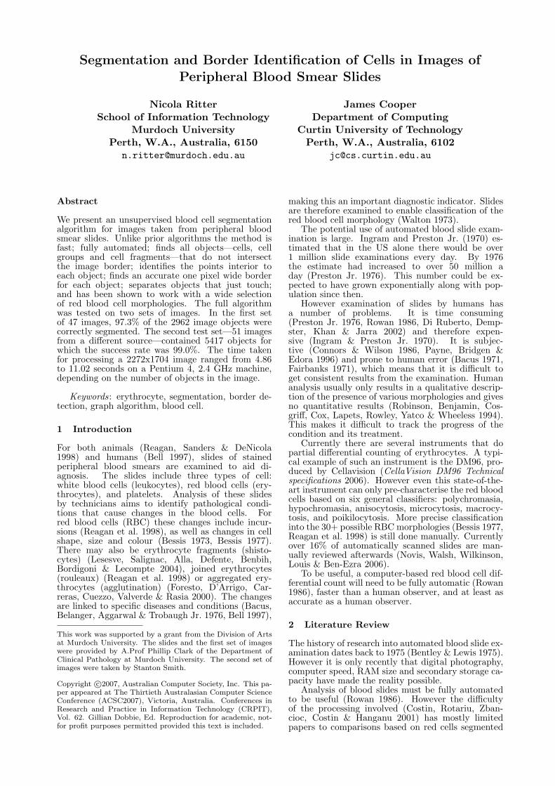
As almost all mammalian red-cells are similar inshape, we use canine blood cell slides for our process-ing as canines have the largest cells of the non-humanmammals (Reagan et al. 1998). Their blood slides arealso more easily obtained than those of human blood.

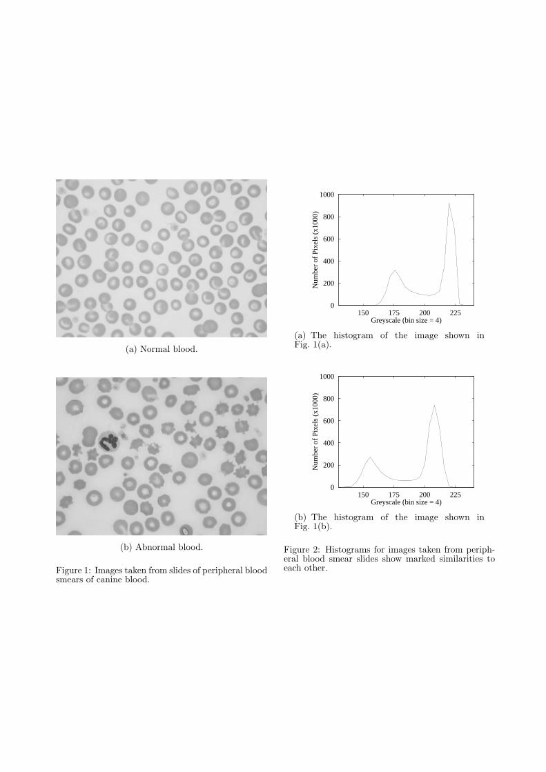
The slides were made using the ‘wedge technique’.They were then air dried, fixed in alcohol and stainedusing Wright’s and Giemsa stain. The slides weremounted in a Nikon eclipse microscope and viewed at100x magnification with oil immersion. Parts of theslide were then digitally photographed using a Nikoncoolpix camera, to give 2272x1704 colour images.The colour images were converted to greyscale to im-prove initial processing time. Figure 1 shows typi-cal greyscale images of canine peripheral blood smearslides. Figure 1(a) shows normal blood and Fig. 1(b)shows blood containing irregularly shaped, damagedred blood cells called acanthocytes. The large cellcontaining darker material—the nucleus—is a whiteblood cell, the smaller diffuse cells are platelets andthe smaller solid pieces are red-cell fragments.

4 A Fully Automated Segmentation andBoundary Identification Algorithm

4.1 Segmentation

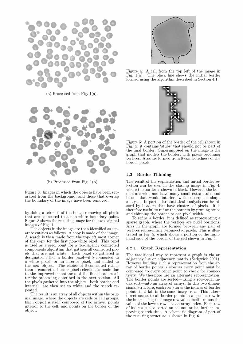
Greyscale histograms of the images in Fig. 1 areshown in Fig. 2. They were calculated using a binsize of 4, which acts to smooth the histogram. Ascan be seen, there is a marked similarity between thehistograms. This similarity holds for all images towhich we have access, suggesting that the histogramscan be used for automatic selection of a useful thresh-old (Weszaka, Nagel & Rosenfeld 1974). This is doneas follows. A search is made from the right to the leftof the histogram, for the first decrease in pixel count.This gives the location of the right peak, which cor-responds to the most common greyscale within thebackground. From there the search continues untilthe first increase in pixel count, which gives the mid-dle low point. As this low point includes pixels thatform part of the border of the cells, the threshold ischosen as the greyscale that falls 1

4 of the ‘distance’from the central minimum towards the right peak.This choice forms a good balance between separationof overlapping cells and ‘leakage’ of the backgroundinto central pale areas close to the border of a cell.

The background of the image is then identi-fied using a 4-adjacency connected components algo-rithm (Gonzalez & Woods 2002) instead of threshold-ing. The initial seed point of this algorithm is the top-left most point in the image with a greyscale greaterthan the calculated threshold. From this seed pointall connected pixels with greyscale greater than thethreshold value are converted to white. To ensurethat the seed point is not interior to a cell, the con-nected pixels are counted. If this number is muchless than the number of pixels between the centralminimum of the histogram and the right most peak,then the algorithm iterates using a new seed point,10 pixels down and to the right of the current seedpoint.

The algorithm results in a segmented image withthe background white and the foreground containingall the cells (red, white and platelets). Incompletecells that overlap the edge of the image are deleted

(a) Normal blood.

(b) Abnormal blood.

Figure 1: Images taken from slides of peripheral bloodsmears of canine blood.

0

200

400

600

800

1000

150 175 200 225N

umbe

r of

Pix

els

(x10

00)

Greyscale (bin size = 4)

(a) The histogram of the image shown inFig. 1(a).

0

200

400

600

800

1000

150 175 200 225

Num

ber

of P

ixel

s (x

1000

)

Greyscale (bin size = 4)

(b) The histogram of the image shown inFig. 1(b).

Figure 2: Histograms for images taken from periph-eral blood smear slides show marked similarities toeach other.

(a) Processed from Fig. 1(a).

(b) Processed from Fig. 1(b)

Figure 3: Images in which the objects have been sep-arated from the background, and those that overlapthe boundary of the image have been removed.

by doing a ‘circuit’ of the image removing all pixelsthat are connected to a non-white boundary point.Figure 3 shows the resulting image for the two originalimages of Fig. 1.

The objects in the image are then identified as sep-arate entities as follows. A copy is made of the image.A search is then made from the top-left most cornerof the copy for the first non-white pixel. This pixelis used as a seed point for a 4-adjacency connectedcomponents algorithm that gathers all connected pix-els that are not white. Each pixel so gathered isdesignated either a border pixel—if 8-connected toa white pixel—or an interior pixel, and added tothe new object. The choice of 8-connected ratherthan 4-connected border pixel selection is made dueto the improved smoothness of the final borders af-ter the processing described in the next section. Allthe pixels gathered into the object—both border andinternal—are then set to white and the search re-peated.

The result is an array of all objects within the orig-inal image, where the objects are cells or cell groups.Each object is itself composed of two arrays: pointsinterior to the cell, and points on the border of theobject.

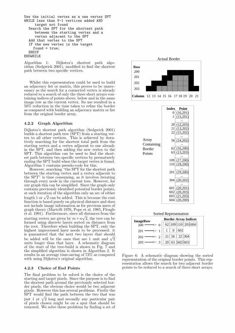
Figure 4: A cell from the top left of the image inFig. 1(a). The black line shows the initial borderformed using the algorithm described in Section 4.1.

Figure 5: A portion of the border of the cell shown inFig. 4: it contains ‘stubs’ that should not be part ofthe final border. Superimposed on the image is thegraph that models the border, with pixels becomingvertices. Arcs are formed from 8-connectedness of theborder pixels.

4.2 Border Thinning

The result of the segmentation and initial border se-lection can be seen in the closeup image in Fig. 4,where the border is shown in black. However the bor-ders are wide and have many small extra stubs andblocks that would interfere with subsequent shapeanalysis. In particular statistical analysis can be bi-ased by borders that have clusters of pixels. It istherefore useful to refine the borders by pruning stubsand thinning the border to one pixel width.

To refine a border, it is defined as representing asparse graph, where the vertices are pixel positions.Arcs in the graph are formed between any pair ofvertices representing 8-connected pixels. This is illus-trated in Fig. 5, which shows a portion of the right-hand side of the border of the cell shown in Fig. 4.

4.2.1 Graph Representation

The traditional way to represent a graph is via anadjacency list or adjacency matrix (Sedgwick 2001).However building such a representation from the ar-ray of border points is slow as every point must becompared to every other point to check for connec-tivity. We therefore use an alternate representation.The border points are sorted—using a row-order in-dex sort—into an array of arrays. In this two dimen-sional structure, each row stores the indices of borderpoints that fall in the same image row. This allowsdirect access to all border points in a specific row inthe image using the image row value itself—minus thevalue of the lowest row—as an array index. Each rowof indices is also sorted on column order, further im-proving search time. A schematic diagram of part ofthe resulting structure is shown in Fig. 6.

Use the initial vertex as a one vertex SPTWHILE less than V-1 vertices added AND

target not foundSearch the SPT for the shortest path

between the starting vertex and avertex adjacent to the SPT

Add that vertex to the SPTIF the new vertex is the target

found = true;ENDIF

ENDWHILE

Algorithm 1: Dijkstra’s shortest path algo-rithm (Sedgwick 2001), modified to find the shortestpath between two specific vertices.

Whilst this representation could be used to buildan adjacency list or matrix, this proves to be unnec-essary as the search for a connected vertex is alreadyreduced to a search of only the three short arrays con-taining indices of points above, below and in the sameimage row as the current vertex. Its use resulted in a50% reduction in the time taken to refine the borderas compared with building an adjacency matrix or listfrom the original border array.

4.2.2 Graph Algorithm

Dijkstra’s shortest path algorithm (Sedgwick 2001)builds a shortest path tree (SPT) from a starting ver-tex to all other vertices. This is achieved by itera-tively searching for the shortest total path from thestarting vertex and a vertex adjacent to one alreadyin the SPT, and then adding the new vertex to theSPT. This algorithm can be used to find the short-est path between two specific vertices by prematurelyending the SPT build when the target vertex is found.Algorithm 1 contains pseudo-code for this.

However, searching “the SPT for the shortest pathbetween the starting vertex and a vertex adjacent tothe SPT” is time consuming, as it involves iteratingthrough every node in the current tree. However, forour graph this can be simplified. Since the graph onlycontains previously identified potential border points,at each iteration of the algorithm only an arc of eitherlength 1 or

√2 can be added. This is because the cost

function is based purely on physical distance and doesnot include image information as for previous users ofgraph theory (Martelli 1976, Pope et al. 1985, Fleagleet al. 1991). Furthermore, since all distances from thestarting vertex are given by m+n

√2, the tree can be

formed using discrete layers sorted on distance fromthe root. Therefore when building the SPT, only thehighest unprocessed layer needs to be processed: itis guaranteed that the next two layers that shouldbe added will be the ones that are 1 unit and

√2

units longer than that layer. A schematic diagramof the start of the tree-build is shown in Fig. 7 andthe simplified algorithm is shown in Algorithm 2. Itresults in an average time-saving of 73% as comparedwith using Dijkstra’s original algorithm.

4.2.3 Choice of End Points

The final problem to be solved is the choice of thestarting and target pixels. Since the purpose is to findthe shortest path around the previously selected bor-der pixels, the obvious choice would be two adjacentpixels. However this has several problems. Firstly theSPT would find the path between the two that wasjust 1 or

√2 long and secondly any particular pair

of pixels chosen might be on a spur that should beremoved. We solve these problems by finding a set of

Sorted Representation

Array ContainingBorderPoints

(21,203)(20,203)

(19,200)

(18,200)

(13,202)

(13,203)

(15,202)

(14,202)

(16,200)

(17,200)

(20,200)

(12,203)

...

...

...

...

...

...

...

(20,201)

(20,202)

601

603602

604

110

304

201

109

6362

56

222120

01

(16,201)(15,201)

Index Point

203

202

200

201

Column 12 13 14 15 16 17 18 19 20 21

Row

Actual Border

109 110 201 604

1 0

62

601

21 56 22 304

20 63 602 603

2

3

1

0200

201

202

203

ImageRow Border Array Indices

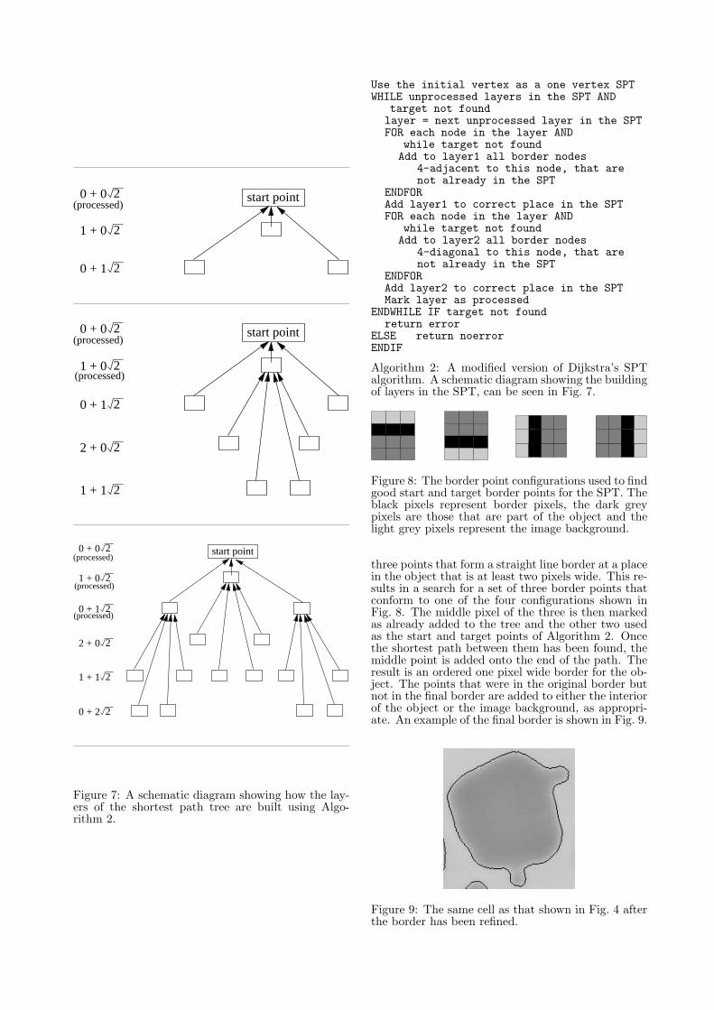
Figure 6: A schematic diagram showing the sortedrepresentation of the original border points. This rep-resentation allows the search for two adjacent borderpoints to be reduced to a search of three short arrays.

(processed)20 + 0

2

2

1 + 0

start point

0 + 1

(processed)

20 + 0

2

2

2

2

1 + 0

start point

0 + 1

2 + 0

1 + 1

(processed)

0 + 2

20 + 0

2

2

2

2

2

1 + 0

start point

0 + 1

2 + 0

1 + 1

(processed)

(processed)

(processed)

Figure 7: A schematic diagram showing how the lay-ers of the shortest path tree are built using Algo-rithm 2.

Use the initial vertex as a one vertex SPTWHILE unprocessed layers in the SPT AND

target not foundlayer = next unprocessed layer in the SPTFOR each node in the layer AND

while target not foundAdd to layer1 all border nodes

4-adjacent to this node, that arenot already in the SPT

ENDFORAdd layer1 to correct place in the SPTFOR each node in the layer AND

while target not foundAdd to layer2 all border nodes

4-diagonal to this node, that arenot already in the SPT

ENDFORAdd layer2 to correct place in the SPTMark layer as processed

ENDWHILE IF target not foundreturn error

ELSE return noerrorENDIF

Algorithm 2: A modified version of Dijkstra’s SPTalgorithm. A schematic diagram showing the buildingof layers in the SPT, can be seen in Fig. 7.

Figure 8: The border point configurations used to findgood start and target border points for the SPT. Theblack pixels represent border pixels, the dark greypixels are those that are part of the object and thelight grey pixels represent the image background.

three points that form a straight line border at a placein the object that is at least two pixels wide. This re-sults in a search for a set of three border points thatconform to one of the four configurations shown inFig. 8. The middle pixel of the three is then markedas already added to the tree and the other two usedas the start and target points of Algorithm 2. Oncethe shortest path between them has been found, themiddle point is added onto the end of the path. Theresult is an ordered one pixel wide border for the ob-ject. The points that were in the original border butnot in the final border are added to either the interiorof the object or the image background, as appropri-ate. An example of the final border is shown in Fig. 9.

Figure 9: The same cell as that shown in Fig. 4 afterthe border has been refined.

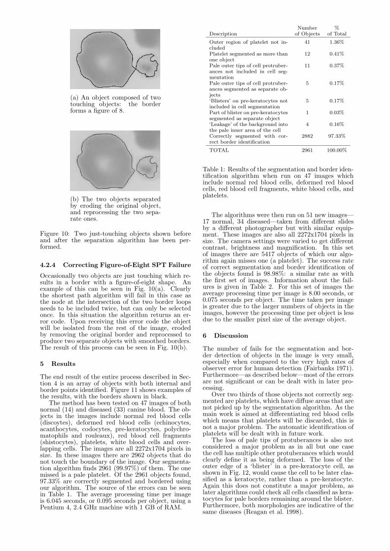
(a) An object composed of twotouching objects: the borderforms a figure of 8.

(b) The two objects separatedby eroding the original object,and reprocessing the two sepa-rate ones.

Figure 10: Two just-touching objects shown beforeand after the separation algorithm has been per-formed.

4.2.4 Correcting Figure-of-Eight SPT Failure

Occasionally two objects are just touching which re-sults in a border with a figure-of-eight shape. Anexample of this can be seen in Fig. 10(a). Clearlythe shortest path algorithm will fail in this case asthe node at the intersection of the two border loopsneeds to be included twice, but can only be selectedonce. In this situation the algorithm returns an er-ror code. Upon receiving this error code the objectwill be isolated from the rest of the image, erodedby removing the original border and reprocessed toproduce two separate objects with smoothed borders.The result of this process can be seen in Fig. 10(b).

5 Results

The end result of the entire process described in Sec-tion 4 is an array of objects with both internal andborder points identified. Figure 11 shows examples ofthe results, with the borders shown in black.

The method has been tested on 47 images of bothnormal (14) and diseased (33) canine blood. The ob-jects in the images include normal red blood cells(discoytes), deformed red blood cells (echinocytes,acanthocytes, codocytes, pre-keratocytes, polychro-matophils and rouleaux), red blood cell fragments(shistocytes), platelets, white blood cells and over-lapping cells. The images are all 2272x1704 pixels insize. In these images there are 2962 objects that donot touch the boundary of the image. Our segmenta-tion algorithm finds 2961 (99.97%) of them. The onemissed is a pale platelet. Of the 2961 objects found,97.33% are correctly segmented and bordered usingour algorithm. The source of the errors can be seenin Table 1. The average processing time per imageis 6.045 seconds, or 0.095 seconds per object, using aPentium 4, 2.4 GHz machine with 1 GB of RAM.

Number %Description of Objects of Total

Outer region of platelet not in-cluded

41 1.36%

Platelet segmented as more thanone object

12 0.41%

Pale outer tips of cell protruber-ances not included in cell seg-mentation

11 0.37%

Pale outer tips of cell protruber-ances segmented as separate ob-jects

5 0.17%

‘Blisters’ on pre-keratocytes notincluded in cell segmentation

5 0.17%

Part of blister on pre-keratocytessegmented as separate object

1 0.03%

‘Leakage’ of the background intothe pale inner area of the cell

4 0.16%

Correctly segmented with cor-rect border identification

2882 97.33%

TOTAL 2961 100.00%

Table 1: Results of the segmentation and border iden-tification algorithm when run on 47 images whichinclude normal red blood cells, deformed red bloodcells, red blood cell fragments, white blood cells, andplatelets.

The algorithms were then run on 51 new images—17 normal, 34 diseased—taken from different slidesby a different photographer but with similar equip-ment. These images are also all 2272x1704 pixels insize. The camera settings were varied to get differentcontrast, brightness and magnification. In this setof images there are 5417 objects of which our algo-rithm again misses one (a platelet). The success rateof correct segmentation and border identification ofthe objects found is 98.98%: a similar rate as withthe first set of images. Information about the fail-ures is given in Table 2. For this set of images theaverage processing time per image is 8.00 seconds, or0.075 seconds per object. The time taken per imageis greater due to the larger numbers of objects in theimages, however the processing time per object is lessdue to the smaller pixel size of the average object.

6 Discussion

The number of fails for the segmentation and bor-der detection of objects in the image is very small,especially when compared to the very high rates ofobserver error for human detection (Fairbanks 1971).Furthermore—as described below—most of the errorsare not significant or can be dealt with in later pro-cessing.

Over two thirds of those objects not correctly seg-mented are platelets, which have diffuse areas that arenot picked up by the segmentation algorithm. As themain work is aimed at differentiating red blood cellswhich means that platelets will be discarded, this isnot a major problem. The automatic identification ofplatelets will be dealt with in future work.

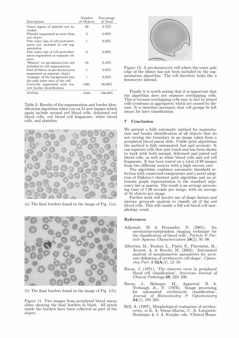
The loss of pale tips of protuberances is also notconsidered a major problem as in all but one casethe cell has multiple other protuberances which wouldclearly define it as being deformed. The loss of theouter edge of a ‘blister’ in a pre-keratocyte cell, asshown in Fig. 12, would cause the cell to be later clas-sified as a keratocyte, rather than a pre-keratocyte.Again this does not constitute a major problem, aslater algorithms could check all cells classified as kera-tocytes for pale borders remaining around the blister.Furthermore, both morphologies are indicative of thesame diseases (Reagan et al. 1998).

Number PercentageDescription of Objects of Total

Outer region of platelet not in-cluded

39 0.72%

Platelet segmented as more thanone object

3 0.06%

Pale outer tips of cell protruber-ances not included in cell seg-mentation

1 0.02%

Pale outer tips of cell protruber-ances segmented as separate ob-jects

0 0.00%

‘Blisters’ on pre-keratocytes notincluded in cell segmentation

10 0.18%

Part of blister on pre-keratocytessegmented as separate object

1 0.02%

‘Leakage’ of the background intothe pale inner area of the cell

1 0.02%

Correctly segmented with cor-rect border identification

5361 98.98%

TOTAL 5416 100.00%

Table 2: Results of the segmentation and border iden-tification algorithm when run on 51 new images whichagain include normal red blood cells, deformed redblood cells, red blood cell fragments, white bloodcells, and platelets.

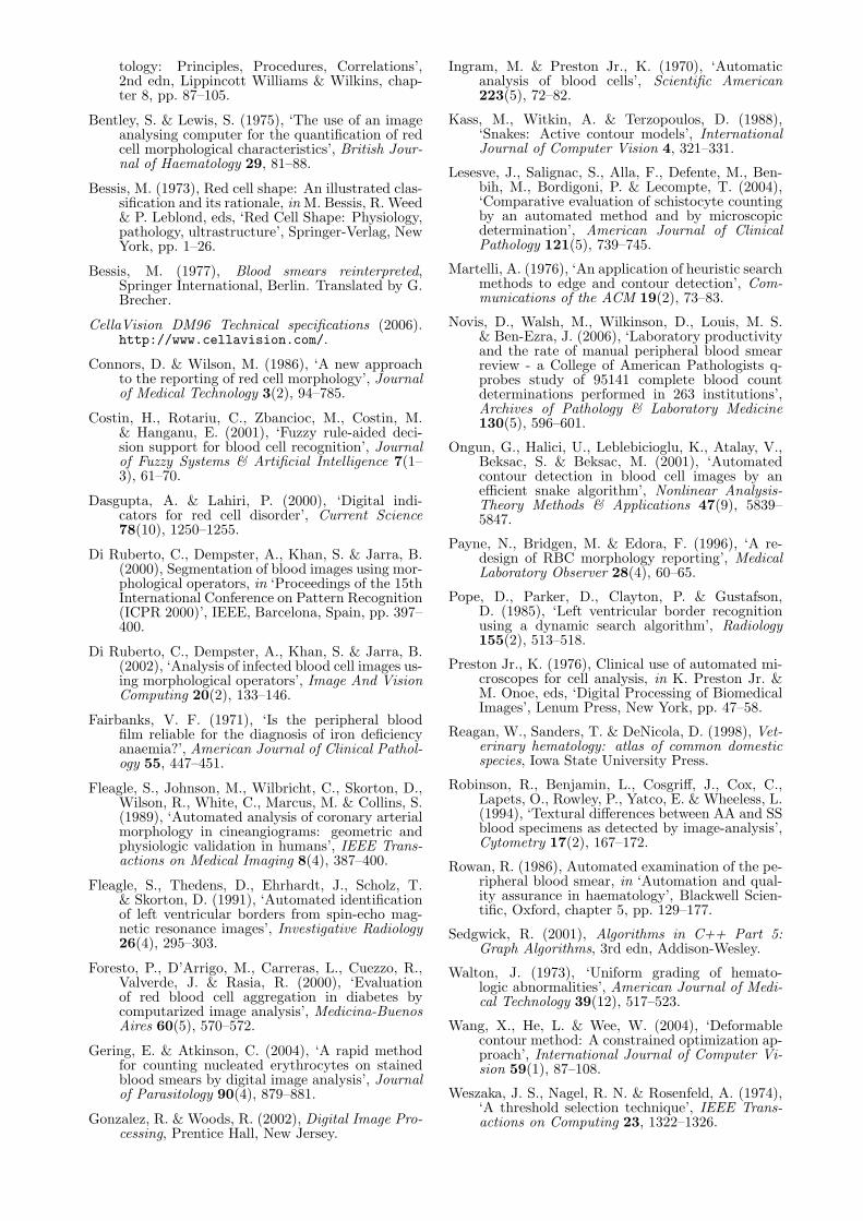
(a) The final borders found in the image of Fig. 1(a).

(b) The final borders found in the image of Fig. 1(b).

Figure 11: Two images from peripheral blood smearslides showing the final borders in black. All pixelsinside the borders have been collected as part of theobject.

Figure 12: A pre-keratocyte cell where the outer paleedge of the blister has not been included by the seg-mentation algorithm. The cell therefore looks like akeratocyte instead.

Finally it is worth noting that it is important thatthe algorithm does not separate overlapping cells.This is because overlapping cells may in fact be joinedcells (rouleaux or aggregates) which are caused by dis-ease. It is therefore necessary that cell groups be leftintact for later classification.

7 Conclusion

We present a fully automatic method for segmenta-tion and border identification of all objects that donot overlap the boundary in an image taken from aperipheral blood smear slide. Unlike prior algorithmsthe method is fully automated, fast and accurate. Itcan separate cells that just touch and has been shownto work with both normal, deformed and joined redblood cells, as well as white blood cells and red cellfragments. It has been tested on a total of 98 imagesfrom two different sources with a high success rate.

The algorithm combines automatic threshold se-lection with connected-components and a novel adap-tion of Dijkstra’s shortest path algorithm and an al-ternate graph representation to the standard adja-cency list or matrix. The result is an average process-ing time of 7.06 seconds per image, with an averageof 84 objects per image.

Further work will involve use of shape factors andinterior greyscale analysis to classify all of the redblood cells. This will enable a full red blood cell mor-phology count.

References

Adjouadi, M. & Fernandez, N. (2001), ‘Anorientation-independent imaging technique forthe classification of blood cells’, Particle & Par-ticle Systems Characterization 18(2), 91–98.

Albertini, M., Teodori, L., Piatti, E., Piacentini, M.,Accorsi, A. & Rocchi, M. (2003), ‘Automatedanalysis of morphometric parameters for accu-rate definition of erythrocyte cell shape’, Cytom-etry Part A 52A(1), 12–18.

Bacus, J. (1971), ‘The observer error in peripheralblood cell classification’, American Journal ofClinical Pathology 59, 223–230.

Bacus, J., Belanger, M., Aggarwal, R. &Trobaugh Jr., F. (1976), ‘Image processingfor automated erythrocyte classification’,Journal of Histocemistry & Cytochemistry24(1), 195–201.

Bell, A. (1997), Morphological evaluation of erythro-cytes, in E. A. Stiene-Martin, C. A. Lotspeich-Steininger & J. A. Koepke, eds, ‘Clinical Hema-

tology: Principles, Procedures, Correlations’,2nd edn, Lippincott Williams & Wilkins, chap-ter 8, pp. 87–105.

Bentley, S. & Lewis, S. (1975), ‘The use of an imageanalysing computer for the quantification of redcell morphological characteristics’, British Jour-nal of Haematology 29, 81–88.

Bessis, M. (1973), Red cell shape: An illustrated clas-sification and its rationale, in M. Bessis, R. Weed& P. Leblond, eds, ‘Red Cell Shape: Physiology,pathology, ultrastructure’, Springer-Verlag, NewYork, pp. 1–26.

Bessis, M. (1977), Blood smears reinterpreted,Springer International, Berlin. Translated by G.Brecher.

CellaVision DM96 Technical specifications (2006).http://www.cellavision.com/.

Connors, D. & Wilson, M. (1986), ‘A new approachto the reporting of red cell morphology’, Journalof Medical Technology 3(2), 94–785.

Costin, H., Rotariu, C., Zbancioc, M., Costin, M.& Hanganu, E. (2001), ‘Fuzzy rule-aided deci-sion support for blood cell recognition’, Journalof Fuzzy Systems & Artificial Intelligence 7(1–3), 61–70.

Dasgupta, A. & Lahiri, P. (2000), ‘Digital indi-cators for red cell disorder’, Current Science78(10), 1250–1255.

Di Ruberto, C., Dempster, A., Khan, S. & Jarra, B.(2000), Segmentation of blood images using mor-phological operators, in ‘Proceedings of the 15thInternational Conference on Pattern Recognition(ICPR 2000)’, IEEE, Barcelona, Spain, pp. 397–400.

Di Ruberto, C., Dempster, A., Khan, S. & Jarra, B.(2002), ‘Analysis of infected blood cell images us-ing morphological operators’, Image And VisionComputing 20(2), 133–146.

Fairbanks, V. F. (1971), ‘Is the peripheral bloodfilm reliable for the diagnosis of iron deficiencyanaemia?’, American Journal of Clinical Pathol-ogy 55, 447–451.

Fleagle, S., Johnson, M., Wilbricht, C., Skorton, D.,Wilson, R., White, C., Marcus, M. & Collins, S.(1989), ‘Automated analysis of coronary arterialmorphology in cineangiograms: geometric andphysiologic validation in humans’, IEEE Trans-actions on Medical Imaging 8(4), 387–400.

Fleagle, S., Thedens, D., Ehrhardt, J., Scholz, T.& Skorton, D. (1991), ‘Automated identificationof left ventricular borders from spin-echo mag-netic resonance images’, Investigative Radiology26(4), 295–303.

Foresto, P., D’Arrigo, M., Carreras, L., Cuezzo, R.,Valverde, J. & Rasia, R. (2000), ‘Evaluationof red blood cell aggregation in diabetes bycomputarized image analysis’, Medicina-BuenosAires 60(5), 570–572.

Gering, E. & Atkinson, C. (2004), ‘A rapid methodfor counting nucleated erythrocytes on stainedblood smears by digital image analysis’, Journalof Parasitology 90(4), 879–881.

Gonzalez, R. & Woods, R. (2002), Digital Image Pro-cessing, Prentice Hall, New Jersey.

Ingram, M. & Preston Jr., K. (1970), ‘Automaticanalysis of blood cells’, Scientific American223(5), 72–82.

Kass, M., Witkin, A. & Terzopoulos, D. (1988),‘Snakes: Active contour models’, InternationalJournal of Computer Vision 4, 321–331.

Lesesve, J., Salignac, S., Alla, F., Defente, M., Ben-bih, M., Bordigoni, P. & Lecompte, T. (2004),‘Comparative evaluation of schistocyte countingby an automated method and by microscopicdetermination’, American Journal of ClinicalPathology 121(5), 739–745.

Martelli, A. (1976), ‘An application of heuristic searchmethods to edge and contour detection’, Com-munications of the ACM 19(2), 73–83.

Novis, D., Walsh, M., Wilkinson, D., Louis, M. S.& Ben-Ezra, J. (2006), ‘Laboratory productivityand the rate of manual peripheral blood smearreview - a College of American Pathologists q-probes study of 95141 complete blood countdeterminations performed in 263 institutions’,Archives of Pathology & Laboratory Medicine130(5), 596–601.

Ongun, G., Halici, U., Leblebicioglu, K., Atalay, V.,Beksac, S. & Beksac, M. (2001), ‘Automatedcontour detection in blood cell images by anefficient snake algorithm’, Nonlinear Analysis-Theory Methods & Applications 47(9), 5839–5847.

Payne, N., Bridgen, M. & Edora, F. (1996), ‘A re-design of RBC morphology reporting’, MedicalLaboratory Observer 28(4), 60–65.

Pope, D., Parker, D., Clayton, P. & Gustafson,D. (1985), ‘Left ventricular border recognitionusing a dynamic search algorithm’, Radiology155(2), 513–518.

Preston Jr., K. (1976), Clinical use of automated mi-croscopes for cell analysis, in K. Preston Jr. &M. Onoe, eds, ‘Digital Processing of BiomedicalImages’, Lenum Press, New York, pp. 47–58.

Reagan, W., Sanders, T. & DeNicola, D. (1998), Vet-erinary hematology: atlas of common domesticspecies, Iowa State University Press.

Robinson, R., Benjamin, L., Cosgriff, J., Cox, C.,Lapets, O., Rowley, P., Yatco, E. & Wheeless, L.(1994), ‘Textural differences between AA and SSblood specimens as detected by image-analysis’,Cytometry 17(2), 167–172.

Rowan, R. (1986), Automated examination of the pe-ripheral blood smear, in ‘Automation and qual-ity assurance in haematology’, Blackwell Scien-tific, Oxford, chapter 5, pp. 129–177.

Sedgwick, R. (2001), Algorithms in C++ Part 5:Graph Algorithms, 3rd edn, Addison-Wesley.

Walton, J. (1973), ‘Uniform grading of hemato-logic abnormalities’, American Journal of Medi-cal Technology 39(12), 517–523.

Wang, X., He, L. & Wee, W. (2004), ‘Deformablecontour method: A constrained optimization ap-proach’, International Journal of Computer Vi-sion 59(1), 87–108.

Weszaka, J. S., Nagel, R. N. & Rosenfeld, A. (1974),‘A threshold selection technique’, IEEE Trans-actions on Computing 23, 1322–1326.