Efficient Identification and Utilization of Spectrum

Opportunities in Cognitive Radio Networks

by

Hyoil Kim

A dissertation submitted in partial fulfillmentof the requirements for the degree of

Doctor of Philosophy(Electrical Engineering: Systems)

in The University of Michigan2010

Doctoral Committee:

Professor Kang G. Shin, ChairAssociate Professor Achilleas AnastasopoulosAssociate Professor Jason N. FlinnAssociate Professor Mingyan Liu

c© Hyoil Kim 2010All Rights Reserved

To my wife Hee Sun, and my parents

ii

ACKNOWLEDGEMENTS

I would like to express my sincere gratitude to Professor Kang G. Shin for his

extraordinary support and guidance during my doctoral studies. He has inspired

me with many critical aspects of becoming a good researcher such as completeness,

imagination, practicality, and agility. He has advised me not only on my research,

but also on my career and life. I thus feel fortunate to work with him and proud

of being a member of his research group, Real-Time Computing Laboratory. I am

also thankful to my research committee, Professor Mingyan Liu, Professor Achil-

leas Anastasopoulos, and Professor Jason N. Flinn for their support and valuable

suggestions on my dissertation.

My special thanks go to my beloved wife, Hee Sun Min, and my parents. Hee

Sun has been my biggest supporter during my doctoral studies enduring hard times

together. I am indebted to my parents for their unconditional love and support

throughout my life. It would not have been possible to stand where I am now

without them.

I feel grateful to Professor Mingyan Liu, Dr. Carlos Cordeiro, Dr. Chun-Ting

Chou, and Professor Demosthenis Teneketzis for serving as my reference. I also thank

my mentors and collaborators, Dr. Bong-Jun Ko at IBM T.J. Watson Research

Center and Dr. Kiran Challapali and Dr. Dave Cavalcanti at Philips Research

North America. My appreciation also goes to Alexander W. Min, Dr. Jaehyuk

Choi, and Ashwini Kumar for their kind support and collaboration in co-authoring

iii

conference and journal papers, and also goes to other former/current members of

RTCL especially Dr. Daji Qiao, Dr. Taejoon Park, Dr. Jai-Jin Lim, Dr. Abhijit

Bose, Dr. Kyu-Han Kim, Dr. Min-gyu Cho, Dr. Pradeep Padala, Dr. Jisoo Yang,

Dr. Bechir Hamdaoui, Dr. Young-June Choi, Dr. Sangsoo Park, Dr. Ji-Hoon Yun,

Eugene Chai, and Xinyu Zhang.

I also want to thank for the financial support from the Korea Science and En-

gineering (KOSEF) scholarship foundation, Samsung scholarship foundation, NSF,

Intel Corporation, Philips Research North America, and NEC Labs North America.

iv

TABLE OF CONTENTS

DEDICATION . . . . . . . . . . . . . . . . . . . . . . . . . . . . . . . . . . ii

ACKNOWLEDGEMENTS . . . . . . . . . . . . . . . . . . . . . . . . . . iii

LIST OF FIGURES . . . . . . . . . . . . . . . . . . . . . . . . . . . . . . . x

LIST OF TABLES . . . . . . . . . . . . . . . . . . . . . . . . . . . . . . . . xiii

ABSTRACT . . . . . . . . . . . . . . . . . . . . . . . . . . . . . . . . . . . xiv

CHAPTER

I. INTRODUCTION . . . . . . . . . . . . . . . . . . . . . . . . . . . 1

1.1 Identification of Spectrum Opportunities . . . . . . . . . . . . 21.2 Utilization of Spectrum Opportunities . . . . . . . . . . . . . 41.3 Overview of Existing Approaches . . . . . . . . . . . . . . . . 6

1.3.1 Discovery of Spectrum Opportunities via Out-of-bandSensing . . . . . . . . . . . . . . . . . . . . . . . . . 6

1.3.2 Incumbent User Protection via In-band Sensing . . 61.3.3 Utilization of Spectrum Opportunities for Profit Max-

imization . . . . . . . . . . . . . . . . . . . . . . . . 71.4 Main Contributions . . . . . . . . . . . . . . . . . . . . . . . 81.5 System Model . . . . . . . . . . . . . . . . . . . . . . . . . . 10

1.5.1 Channel Model . . . . . . . . . . . . . . . . . . . . 101.5.2 Sensing Model . . . . . . . . . . . . . . . . . . . . . 12

1.6 Organization of the Dissertation . . . . . . . . . . . . . . . . 13

II. OUT-OF-BAND SENSING PART I: MAXIMAL DISCOV-ERY OF SPECTRUM OPPORTUNITIES . . . . . . . . . . . 14

2.1 Introduction . . . . . . . . . . . . . . . . . . . . . . . . . . . 142.1.1 Contributions . . . . . . . . . . . . . . . . . . . . . 162.1.2 Organization . . . . . . . . . . . . . . . . . . . . . . 17

2.2 Related Work . . . . . . . . . . . . . . . . . . . . . . . . . . . 172.3 System Model . . . . . . . . . . . . . . . . . . . . . . . . . . 18

v

2.3.1 Network Topology . . . . . . . . . . . . . . . . . . . 182.3.2 Channel and Sensing Model . . . . . . . . . . . . . 182.3.3 Opportunity-Usage Model . . . . . . . . . . . . . . 19

2.4 Maximal Discovery of Opportunities by Optimizing Sensing-Period . . . . . . . . . . . . . . . . . . . . . . . . . . . . . . . 20

2.4.1 Analysis of UOPP i(T iP ) . . . . . . . . . . . . . . . . 21

2.4.2 Analysis of SSOH i(TP) . . . . . . . . . . . . . . . 252.4.3 Sensing-Period Optimization Algorithm . . . . . . . 26

2.5 Channel-Parameter Estimation . . . . . . . . . . . . . . . . . 262.5.1 Maximum Likelihood (ML) Estimators . . . . . . . 272.5.2 Confidence Interval of Estimators . . . . . . . . . . 292.5.3 Estimation on Time-Varying Channels . . . . . . . 32

2.6 Performance Evaluation . . . . . . . . . . . . . . . . . . . . . 322.6.1 Simulation Setup . . . . . . . . . . . . . . . . . . . 322.6.2 The Simulation Results . . . . . . . . . . . . . . . . 34

2.7 Deployment Scenarios . . . . . . . . . . . . . . . . . . . . . . 372.7.1 Application to IEEE 802.11 . . . . . . . . . . . . . . 382.7.2 Application to licensed bands . . . . . . . . . . . . . 39

2.8 Conclusion . . . . . . . . . . . . . . . . . . . . . . . . . . . . 39

III. OUT-OF-BAND SENSING PART II: FAST DISCOVERYOF SPECTRUM OPPORTUNITIES . . . . . . . . . . . . . . . 40

3.1 Introduction . . . . . . . . . . . . . . . . . . . . . . . . . . . 403.1.1 Contributions . . . . . . . . . . . . . . . . . . . . . 413.1.2 Organization . . . . . . . . . . . . . . . . . . . . . . 42

3.2 Related Work . . . . . . . . . . . . . . . . . . . . . . . . . . . 423.3 System Model . . . . . . . . . . . . . . . . . . . . . . . . . . 44

3.3.1 Network Model . . . . . . . . . . . . . . . . . . . . 443.3.2 Channel and Sensing Model . . . . . . . . . . . . . 453.3.3 Notation Table . . . . . . . . . . . . . . . . . . . . . 45

3.4 Sequential Sensing Mechanism . . . . . . . . . . . . . . . . . 453.4.1 Opportunity Discovery Procedure . . . . . . . . . . 463.4.2 Channel Idle Probability Prediction . . . . . . . . . 48

3.5 Optimal Sensing Sequence for Minimal Opportunity-DiscoveryLatency . . . . . . . . . . . . . . . . . . . . . . . . . . . . . . 51

3.5.1 Problem Statement . . . . . . . . . . . . . . . . . . 513.5.2 Offline vs. Online Sensing Sequences . . . . . . . . . 523.5.3 Optimal Online Sensing Sequence Algorithm . . . . 553.5.4 Efficient Suboptimal Sensing Sequence Algorithm . 603.5.5 Discussion . . . . . . . . . . . . . . . . . . . . . . . 61

3.6 Backup Channel List Management . . . . . . . . . . . . . . . 633.6.1 Construction of Initial BCL . . . . . . . . . . . . . 643.6.2 Periodic BCL Update . . . . . . . . . . . . . . . . . 65

vi

3.7 Channel-Parameter Estimation . . . . . . . . . . . . . . . . . 673.7.1 Single-Step Bayesian Inference . . . . . . . . . . . . 683.7.2 Iterative Bayesian Inference . . . . . . . . . . . . . 683.7.3 Complexity Reduction . . . . . . . . . . . . . . . . 71

3.8 Performance Evaluation . . . . . . . . . . . . . . . . . . . . . 723.8.1 Test 1: Performance of Proposed Sequence . . . . . 743.8.2 Test 2: BCL Update vs. No BCL Update . . . . . . 75

3.9 Conclusion . . . . . . . . . . . . . . . . . . . . . . . . . . . . 76

IV. IN-BAND SENSING: PROTECTION OF LEGACY SPEC-TRUM USERS . . . . . . . . . . . . . . . . . . . . . . . . . . . . . 79

4.1 Introduction . . . . . . . . . . . . . . . . . . . . . . . . . . . 794.1.1 Sensor Clustering . . . . . . . . . . . . . . . . . . . 804.1.2 Scheduling of In-band Sensing . . . . . . . . . . . . 814.1.3 False Detection vs. Efficient Channel-Reuse . . . . . 824.1.4 Organization . . . . . . . . . . . . . . . . . . . . . . 83

4.2 Related Work . . . . . . . . . . . . . . . . . . . . . . . . . . . 844.3 System Model . . . . . . . . . . . . . . . . . . . . . . . . . . 84

4.3.1 IEEE 802.22 . . . . . . . . . . . . . . . . . . . . . . 844.3.2 Channel and Sensing Model . . . . . . . . . . . . . 86

4.4 Spectrum Sensor Clustering . . . . . . . . . . . . . . . . . . . 884.4.1 Cluster Size . . . . . . . . . . . . . . . . . . . . . . 884.4.2 Sensor Density . . . . . . . . . . . . . . . . . . . . . 904.4.3 Discussion . . . . . . . . . . . . . . . . . . . . . . . 91

4.5 Scheduling of In-band Sensing . . . . . . . . . . . . . . . . . 934.5.1 Sensing Requirements in IEEE 802.22 . . . . . . . . 944.5.2 TSS mechanism in IEEE 802.22 . . . . . . . . . . . 954.5.3 In-band Sensing Scheduling Algorithm . . . . . . . . 95

4.6 Feasibility of Energy Detection . . . . . . . . . . . . . . . . . 1004.6.1 Two Important Factors in In-band Sensing . . . . . 1004.6.2 Optimal Sensing Time and Frequency . . . . . . . . 1044.6.3 Energy Detection vs. Feature Detection . . . . . . . 1094.6.4 Minimum Number of Sensors for Feasible Energy

Detection at aRSS = IDT . . . . . . . . . . . . . . 1114.7 Effective Channel-Reuse Time . . . . . . . . . . . . . . . . . 1124.8 Conclusion . . . . . . . . . . . . . . . . . . . . . . . . . . . . 115

V. WHITESPACE UTILIZATION PART I: OPTIMAL CON-TROL OF SECONDARY USERS FOR PROFIT MAXI-MIZATION AT CR SERVICE PROVIDERS . . . . . . . . . . 117

5.1 Introduction . . . . . . . . . . . . . . . . . . . . . . . . . . . 1175.1.1 Contributions . . . . . . . . . . . . . . . . . . . . . 119

vii

5.1.2 Organization . . . . . . . . . . . . . . . . . . . . . . 1215.2 Related Work . . . . . . . . . . . . . . . . . . . . . . . . . . . 1215.3 System Model . . . . . . . . . . . . . . . . . . . . . . . . . . 122

5.3.1 Channel Model . . . . . . . . . . . . . . . . . . . . 1225.3.2 Spectrum Auction Model . . . . . . . . . . . . . . . 1235.3.3 Multi-class User QoS Model . . . . . . . . . . . . . 1245.3.4 End-User Pricing Model . . . . . . . . . . . . . . . 125

5.4 SMDP Formulation . . . . . . . . . . . . . . . . . . . . . . . 1265.4.1 System State and State Space . . . . . . . . . . . . 1265.4.2 Possible Actions and Action Space . . . . . . . . . . 1275.4.3 Validity of SMDP Formulation . . . . . . . . . . . . 1295.4.4 Decision Epochs . . . . . . . . . . . . . . . . . . . . 1315.4.5 State-Transition Probability . . . . . . . . . . . . . 1325.4.6 Revenue and Reimbursement Cost . . . . . . . . . . 133

5.5 Optimal User Control via a Linear Programming Algorithm . 1345.5.1 Linear Programming SMDP Algorithm: Constrained

QoS . . . . . . . . . . . . . . . . . . . . . . . . . . . 1345.5.2 Complexity of SMDP Algorithm . . . . . . . . . . . 137

5.6 Prioritized Multi-Class User Control . . . . . . . . . . . . . . 1385.7 Performance Evaluation . . . . . . . . . . . . . . . . . . . . . 141

5.7.1 System State Transition by Optimal Control . . . . 1425.7.2 Approximation Accuracy of Eq. (5.5) . . . . . . . . 1425.7.3 Achieved Optimal Profit by SMDP Algorithm . . . 1435.7.4 Tradeoffs between Two QoS Constraints . . . . . . . 147

5.8 Conclusion . . . . . . . . . . . . . . . . . . . . . . . . . . . . 149

VI. WHITESPACE UTILIZATION PART II: PRICE AND QUAL-ITY COMPETITION BETWEEN CR SERVICE PROVIDERS150

6.1 Introduction . . . . . . . . . . . . . . . . . . . . . . . . . . . 1506.1.1 Contributions . . . . . . . . . . . . . . . . . . . . . 1526.1.2 Organization . . . . . . . . . . . . . . . . . . . . . . 153

6.2 Related Work . . . . . . . . . . . . . . . . . . . . . . . . . . . 1536.3 System Model . . . . . . . . . . . . . . . . . . . . . . . . . . 154

6.3.1 Channel Model . . . . . . . . . . . . . . . . . . . . 1546.3.2 Auction Model . . . . . . . . . . . . . . . . . . . . . 1556.3.3 Service Model . . . . . . . . . . . . . . . . . . . . . 155

6.4 Two-Stage Market Competition . . . . . . . . . . . . . . . . . 1586.5 Price Competition Analysis . . . . . . . . . . . . . . . . . . . 161

6.5.1 Three Pricing Strategies . . . . . . . . . . . . . . . 1616.5.2 Optimal Price Strategy . . . . . . . . . . . . . . . . 1626.5.3 Nash Equilibrium of the Price Competition . . . . . 165

6.6 Quality Competition Analysis . . . . . . . . . . . . . . . . . . 1666.6.1 Market entry barrier . . . . . . . . . . . . . . . . . 167

viii

6.6.2 Region-specific optimal quality strategies . . . . . . 1686.6.3 Optimal quality strategy . . . . . . . . . . . . . . . 1706.6.4 Discussion . . . . . . . . . . . . . . . . . . . . . . . 172

6.7 Evaluation of Wi-Fi 2.0 Network Dynamics . . . . . . . . . . 1736.7.1 Approximation accuracy in state decomposition . . 1736.7.2 Impact of arrival rate and leasing cost . . . . . . . . 1746.7.3 Impact of eviction cost . . . . . . . . . . . . . . . . 175

6.8 Conclusion . . . . . . . . . . . . . . . . . . . . . . . . . . . . 175

VII. Conclusion and Future Direction . . . . . . . . . . . . . . . . . 178

7.1 Research Contributions . . . . . . . . . . . . . . . . . . . . . 1787.1.1 Contributions in Opportunity Discovery . . . . . . . 1787.1.2 Contributions in Opportunity Utilization . . . . . . 180

7.2 Future Direction . . . . . . . . . . . . . . . . . . . . . . . . . 1817.2.1 Energy-efficient Spectrum-agile Networking . . . . . 1817.2.2 Coexistence of Heterogeneous Wireless Networks . . 1817.2.3 Seamless Multimedia Communications . . . . . . . . 182

APPENDIX . . . . . . . . . . . . . . . . . . . . . . . . . . . . . . . . . . . . 183

BIBLIOGRAPHY . . . . . . . . . . . . . . . . . . . . . . . . . . . . . . . . 185

ix

LIST OF FIGURES

Figure

1.1 An illustration of spectrum opportunities. . . . . . . . . . . . . . . . 2

1.2 An overview of the dissertation. . . . . . . . . . . . . . . . . . . . . 10

1.3 Channel model in terms of an ON/OFF alternating renewal process 11

1.4 Spectrum sensing model with sensing-period T iP and sensing-time T i

I 12

2.1 An example of periodic sensing . . . . . . . . . . . . . . . . . . . . 15

2.2 The concept of SSOH i: channel 1’s discovered opportunity cannotbe utilized during sensing of channel 2 . . . . . . . . . . . . . . . . 21

2.3 Illustration of T i0(t), T i

1(t), T i0(t) and T i

1(t) - x/y denotes the remain-ing time in the current OFF/ON period starting from ts. In case thestate transition occurs at ts, x/y is used instead of x/y. . . . . . . . 22

2.4 The density function of the remaining time in the current OFF period 23

2.5 The observed channel-usage pattern model . . . . . . . . . . . . . . 26

2.6 The graph of P i01(T

iP ) and upper bound of T i

P . . . . . . . . . . . . 31

2.7 Achieved opportunity ratio (AOR) . . . . . . . . . . . . . . . . . . . 36

2.8 Adaptation of sensing-periods (N=3 case: channel 1) . . . . . . . . 36

2.9 Estimation of unknown channel parameters: N=3 case . . . . . . . 37

3.1 An illustration of opportunity discovery when a CRN requires twoidle channels for its operation. . . . . . . . . . . . . . . . . . . . . . 47

3.2 Pseudo-code of the dynamic programming (DP) search algorithm(S∗: optimal sequence) . . . . . . . . . . . . . . . . . . . . . . . . . 56

x

3.3 Pseudo-code of the proposed suboptimal sensing sequence algorithm(S∗: near-optimal sequence) . . . . . . . . . . . . . . . . . . . . . . 62

3.4 Transition of channel association . . . . . . . . . . . . . . . . . . . . 64

3.5 Iterative Bayesian inference . . . . . . . . . . . . . . . . . . . . . . 69

3.6 Test 1: performance of the proposed sequences . . . . . . . . . . . . 77

3.7 Test 2: proposed BCL update vs. no update . . . . . . . . . . . . . 78

4.1 Illustration of an IEEE 802.22 WRAN . . . . . . . . . . . . . . . . 85

4.2 An illustration of clustered sensor networks . . . . . . . . . . . . . . 89

4.3 An example hexagonal sensor deployment . . . . . . . . . . . . . . . 91

4.4 An example of periodic sensing when a channel transits from OFFto ON due to the returning PUs . . . . . . . . . . . . . . . . . . . . 97

4.5 The in-band sensing scheduling algorithm . . . . . . . . . . . . . . . 99

4.6 Performance comparison (in PMD(N)) of energy detection: AWGNchannel and shadow-fading channel . . . . . . . . . . . . . . . . . . 102

4.7 Inter-cell interference scenarios in 802.22 . . . . . . . . . . . . . . . 104

4.8 The worst-case channel assignment to have maximal inter-cell inter-ference . . . . . . . . . . . . . . . . . . . . . . . . . . . . . . . . . . 104

4.9 Energy detection: sensing-overhead and sensing-frequency . . . . . . 106

4.10 Pilot detection: sensing-overhead and sensing-frequency . . . . . . . 107

4.11 Energy detection vs. pilot detection: location of aRSSthreshold . . . . 108

4.12 Number of sensors (i.e., N) vs. optimal sensing-overhead (aRSS =IDT , 1 dB noise uncertainty) . . . . . . . . . . . . . . . . . . . . . 112

4.13 Treuse, Nmin, and sensing overhead TI/TP with varying PmaxFA . . . . 116

5.1 Inter-plane interactions in the dynamic spectrum market . . . . . . 118

xi

5.2 The preemptive spectrum lease model . . . . . . . . . . . . . . . . . 120

5.3 Time-varying channel capacity . . . . . . . . . . . . . . . . . . . . . 123

5.4 An example of channel allocation with M = 2, K = 3, and C = 5. . 125

5.5 The size of the search space according to (M ,K) . . . . . . . . . . . 138

5.6 The state-transition diagrams of the proposed SMDP algorithm, ac-cording to user arrivals (shown for m = 2) . . . . . . . . . . . . . . 143

5.7 Approximation accuracy of Eq. (5.5) for two types of ON/OFF dis-tributions . . . . . . . . . . . . . . . . . . . . . . . . . . . . . . . . 144

5.8 Comparison of SMDP and two variations of CS in terms of theirachieved profits . . . . . . . . . . . . . . . . . . . . . . . . . . . . . 145

5.9 Optimal profit with various end-user pricing . . . . . . . . . . . . . 147

5.10 The tradeoffs between Pb and Pd . . . . . . . . . . . . . . . . . . . . 148

6.1 The three-tier Wi-Fi 2.0 market . . . . . . . . . . . . . . . . . . . . 151

6.2 The preemptive lease model with ON-OFF channels . . . . . . . . . 153

6.3 A duopoly Wi-Fi 2.0 network . . . . . . . . . . . . . . . . . . . . . 156

6.4 State transition of WSP i’s system . . . . . . . . . . . . . . . . . . 159

6.5 Nash Equilibrium of the price competition . . . . . . . . . . . . . . 163

6.6 Five decision regions of (u1, u2) . . . . . . . . . . . . . . . . . . . . 168

6.7 The Nash Equilibrium of the quality competition . . . . . . . . . . 171

6.8 Decomposition approximation accuracy . . . . . . . . . . . . . . . . 174

6.9 Fundamental tradeoffs in the duopoly market . . . . . . . . . . . . . 177

xii

LIST OF TABLES

Table

2.1 General evaluation parameters . . . . . . . . . . . . . . . . . . . . . 34

2.2 AOR test parameters . . . . . . . . . . . . . . . . . . . . . . . . . . 34

2.3 Channel-usage pattern parameters . . . . . . . . . . . . . . . . . . . 34

3.1 Summary of notations . . . . . . . . . . . . . . . . . . . . . . . . . 46

3.2 Test-specific simulation parameters, i ∈ {1, . . . , M} . . . . . . . . . 73

4.1 Incumbent detection threshold (IDT ) of primary signals . . . . . . 92

4.2 RSS thresholds under various noise uncertainty . . . . . . . . . . . . 109

4.3 RSS thresholds under various inter-CRN interference . . . . . . . . 110

4.4 The minimum number of sensor (Nmin) necessary for energy detec-tion to become feasible at aRSS = IDT . . . . . . . . . . . . . . . 111

5.1 The list of common test parameters . . . . . . . . . . . . . . . . . . 142

5.2 The list of test-specific parameters . . . . . . . . . . . . . . . . . . . 142

xiii

ABSTRACT

There has been an exponential increase in spectrum demands due to new emerging

wireless services and applications, making it harder to find unallocated spectrum

bands for future usage. This potential resource scarcity is rooted at inefficient uti-

lization of spectrum under static spectrum allocation. Therefore, a new concept

of dynamic spectrum access (DSA) has been proposed to opportunistically utilize

the legacy spectrum bands by cognitive radio (CR) users. Cognitive radio is a key

technology for alleviating this inefficient spectrum utilization, since it can help dis-

cover spectrum opportunities (or whitespaces) in which legacy spectrum users do not

temporarily use their assigned spectrum bands.

In a DSA network, it is crucial to efficiently identify and utilize the whitespaces.

We address this issue by considering spectrum sensing and resource allocation. Spec-

trum sensing is to discover spectrum opportunities and to protect the legacy users

(or incumbents) against harmful interference from the CR users. In particular, sens-

ing is an interaction between PHY and MAC layers where in the PHY-layer signal

detection is performed, and in the MAC-layer spectrum sensing is scheduled and spec-

trum sensors are coordinated for collaborative sensing. Specifically, we propose an

efficient MAC-layer sensing scheduling algorithm that discovers spectrum opportuni-

ties as much as possible for better quality-of-service (QoS), and as fast as possible for

seamless service provisioning. In addition, we propose an optimal in-band spectrum

sensing algorithm to protect incumbents by achieving the detectability requirements

set by regulators (e.g., FCC) while incurring minimal sensing overhead.

xiv

For better utilization of discovered spectrum opportunities, we pay our attention

to resource allocation in the secondary spectrum market where legacy license holders

temporarily lease their own spectrum to secondary wireless service providers (WSPs)

for opportunistic spectrum access by CR users. In this setting, we investigate how a

secondary WSP can maximize its profit by optimally controlling the admission and

eviction of its customers (i.e., CR users). In addition, we also focus on the price

and quality competition between co-located WSPs where they contend for enticing

customers by providing more competitive service fee while leasing the channels with

best matching quality.

xv

CHAPTER I

INTRODUCTION

Over the last two decades, there has been an exponential increase in spectrum

demands due to the new emerging wireless services, which causes a shortage of al-

locatable wireless spectrum resources. According to the current static spectrum

allocation policy, each new wireless service/protocol should be assigned a spectrum

band which has never been allocated, and therefore most parts of the spectrum under

3GHz are now allocated to specific use. Although wireless spectrum is considered

in theory an unlimited resource, its poor transmission characteristics at higher fre-

quency bands (e.g., 60GHz) restrict their usage to specific applications (e.g., personal

area networks). As a result, in the near future we expect a shortage of allocatable

spectrum bands with fair transmission characteristics.

This potential resource scarcity is actually solvable, since the shortage derives

from inefficient utilization of spectrum by the static spectrum allocation. A recent

measurement study [55] revealed that the average spectrum utilization is only about

5.2% over time for spectrum bands under 3GHz, measured at many geographical

locations. Nevertheless, the remaining unused portion of time in those bands cannot

be used for other purposes, since the current static policy strictly prohibits such

usage. Therefore, since 2000, FCC has been searching for a new spectrum policy to

1

Channel (frequency)

Wide-band

devices

Time

Power

Narrow-band

devices

PU’s activity

Spectrum opportunities

(white spaces)

Figure 1.1: An illustration of spectrum opportunities.

dynamically utilize the legacy spectrum bands [24–28].

Dynamic Spectrum Access (DSA) is a new paradigm for alleviating the inefficient

spectrum-utilization problem by exploiting the spectrum agility (SA) feature of the

Cognitive Radio (CR) technology. In DSA, (unlicensed) secondary users (SUs) form a

CR network (CRN) and are allowed to opportunistically utilize the spectrum bands

of (licensed) primary users (PUs) as long as the SUs do not cause any harmful

interference to the PUs. The time period when SUs can reuse a licensed band is

called spectrum opportunity or spectrum whitespaces (WS) [41]. Spectrum agility

becomes realizable with the recent progress in wireless communications, such as

Software Defined Radios (SDRs) and smart antennas. The concept of spectrum

opportunity is illustrated in Fig. 1.1.

1.1 Identification of Spectrum Opportunities

It is crucial for CRNs to identify spectrum opportunities efficiently and correctly,

for which spectrum sensing is essential. Spectrum sensing is an act of monitoring a

spectrum band/channel1 for a pre-determined amount of time (called sensing-time)

to detect PU signals in order to determine its availability to SUs. The sensing-time

1The terms spectrum band and channel are used interchangeably throughout the dissertation.

2

depends on the characteristics of PU signals as well as the detection method used.

A single measurement result is called a sample, indicating whether a channel is busy

or idle. Once a channel is sensed idle (i.e., no PU signal is present), it can be utilized

by SUs until its PUs return to the channel.

Spectrum sensing can be realized as a two-layer mechanism. The PHY-layer sens-

ing focuses on efficiently detecting PU signals to identify opportunities by properly

choosing its detection method. Several well-known PHY-layer detection methods,

such as energy detection, matched filter and feature detection [7, 73, 91], have been

proposed as candidates for the PHY-layer sensing. On the other hand, the MAC-

layer sensing generally focuses on two issues: (1) scheduling of sensing, and (2)

collaboration between sensors. Sensing scheduling tries to determine when to sense

and which channel to sense. Sensor collaboration implies concurrent sensing, where

multiple sensors participate in sensing the same channel simultaneously to enhance

the detectability of PU signals.

Sensing can also be categorized into two types: in-band sensing performed on in-

band channels, and out-of-band sensing performed on out-of-band channels. Here,

in-band channels refer to those channels currently in use by SUs; all others are

referred to as out-of-band channels . In-band sensing focuses on protecting PUs via

fast detection of PUs returning to in-band channels. Since the PUs are given priority

in accessing their own channel, SUs must vacate the channel as soon as they detect

the PUs (called channel vacation). Next, out-of-band sensing focuses on providing

enough bandwidth for quality-of-service (QoS) provisioning to SUs, by discovering

spectrum opportunities from out-of-band channels. Out-of-band sensing is further

divided into two types, periodic and reactive sensing, where the choice of a sensing

mode (i.e., periodic vs. reactive) depends on how much demand for opportunities

3

there exists in CRNs.

The two objectives of spectrum sensing, protecting PUs and promoting QoS of

SUs, often conflict. For maximal protection of PUs, it is desirable to perform in-band

sensing as frequently as possible, so that latency of detecting the returning PUs can

be minimized. Such in-band sensing, however, often incurs high sensing-overhead fre-

quently interrupting data transmission between SUs. Therefore, triggering in-band

sensing only if necessary is key to both protect PUs and promote SUs’ QoS. On the

other hand, out-of-band sensing should not be performed more than necessary, be-

cause it forces SUs to reconfigure their antenna frequency to an out-of-band channel

and thus interrupts their in-band transmission.

In this dissertation, we propose medium access control (MAC) layer schemes that

efficiently schedule in-band and out-of-band spectrum sensing so that PUs can be

protected from harmful interference while QoS of SUs can be properly supported.

Specifically, we try to address the following two issues in out-of-band sensing: (1)

how to maximize the amount of opportunities discovered by sensing, and (2) how

to minimize the latency in finding additional opportunities when needed. In terms

of in-band sensing, we focus on how to achieve the maximal protection of legacy

spectrum users while incurring sensing overhead as minimal as possible.

1.2 Utilization of Spectrum Opportunities

Efficient utilization of the discovered spectrum opportunities is also important

since the major objective of DSA is to enhance the overall utilization of legacy

spectrum. In particular, we address this issue in the context of secondary spectrum

market. In a DSA network, the primary license holders may temporarily transfer

their spectrum usage rights to CR users [5, 10] via the secondary spectrum market.

4

The license holders can temporarily lease their channels to the CR users and generate

additional revenue by charging for their opportunistic use of paid-but-idle channels.

The CR end-users can also benefit from this because they can access the spectrum

at a much lower cost than legacy services. However, the CR users are allowed to use

the leased channels only when they are not occupied by the licensed (or primary)

users because the licensed users are given priority over the CR end-users.

The Dynamic Spectrum Market (DSM) is a secondary spectrum market that facil-

itates the transfer of spectrum rights via an auction mechanism. DSM is composed of

three interacting layers/planes: spectrum plane, service plane, and user plane [10,72].

The spectrum is auctioned by a Spectrum Broker (SB) at the top plane where bidders

are the secondary wireless service providers (WSPs) at the middle plane [6,86]. Here,

the SB might be either the regulatory authorities (e.g., FCC in USA and Ofcom in

UK) or an authorized third-party. A secondary WSP leases spectrum via auction

and subleases a portion of the leased channels to the CR end-users at the bottom

plane [44].

This dissertation focuses on two issues in DSM: (1) how a secondary WSP can

maximize its profit by user admission and eviction control when the spectrum de-

mand varies with CR users and applications, e.g., audio/video users will need more

spectrum bandwidth than text only users, and (2) how co-located WSPs can compete

for the price of their service in the customer market and the quality of the leased

spectrum in the auction market.

5

1.3 Overview of Existing Approaches

1.3.1 Discovery of Spectrum Opportunities via Out-of-band Sensing

The following papers are related to the issue of maximal discovery of opportu-

nities. Chou [14] proposed a proactive sensing algorithm with non-adaptive and

randomly-chosen sensing periods. Zhao et al. [99] introduced a Decentralized Cog-

nitive MAC (DC-MAC) with reactive sensing focusing on slotted-time CSMA-based

channel access with synchronized slot information. Sankaranarayanan et al. [71] pro-

posed an Ad-hoc Secondary system MAC (AS-MAC) which is a proactive scheme

with slotted-time-based channel access.

In the context of fast discovery of opportunities, Jiang et al. [45] investigated the

optimal sensing sequence in a multi-channel cognitive MAC protocol, and Shu and

Krunz [81] studied the problem of sequential sensing for throughput efficiency along

with finding the optimal sensing time. Lai et al. [53] considered a scenario in which

SUs can sense more than one channel simultaneously and utilize all discovered idle

channels for their transmission.

1.3.2 Incumbent User Protection via In-band Sensing

There have been many proposals to protect incumbent users via PHY-layer signal

detection schemes such as energy detection [35, 77, 90] and feature detection [13, 18,

36,78]. However, such numerous existing studies are based on the single-time signal

detection, which can be greatly enhanced by the MAC-layer support such as sensing

scheduling and sensor clustering.

Scheduling of sensing in-band channels is to immediately detect returning PUs to

the in-band channels. For example, Cordeiro et al. [18] evaluated the performance of

fast sensing in 802.22 by scheduling it (1 ms) every 40 ms, but they did not optimize

6

the sensing-time and sensing-period. Hoang and Liang [42] introduced an adaptive

sensing scheduling method to capture the tradeoff between SUs’ data-transmission

and spectrum-sensing.

There have also been continuing discussions on use of clustered sensor networks.

Chen et al. [13] proposed a mechanism to form a cluster among neighboring nodes and

then interconnect such clusters. Pawelczak et al. [62] proposed cluster-based sensor

networks to reduce the latency in reporting sensor measurements by designating the

cluster head as a local decision maker. Sun et al. [88] enhanced performance by

clustering sensors where the benefit comes from cluster and sensor diversities.

1.3.3 Utilization of Spectrum Opportunities for Profit Maximization

Once spectrum sensing discovers spectrum opportunities, they can be utilized

by CRNs for various purposes. In particular, this dissertation discusses the eco-

nomic aspects of the whitespace utilization in terms of profit maximization of WSPs.

The profit maximization can be achieved by considering two necessary techniques:

CR user control in terms of customer admission and eviction, and the competition

between co-located WSPs.

The following papers are related to the admission and eviction control of CR users,

although none of them have discussed both types of control in the same context.

Ishibashi et al. [43] considered multi-homed primary users, where a primary user is

either classical or cognitive. However, the classical primaries are assumed not to have

priority over the cognitive primaries, thus unaccounting for channel eviction. Wang et

al. [95] proposed a primary-prioritized Markov approach where primary users have

exclusive rights to access their own channels, without considering the admission

control. Ross and Tsang [66] addressed the problem of optimal admission control

7

on user arrivals with various spectrum demands, in the framework of traditional

networks where the channels are always available without any time-varying patterns.

In the DSM, co-located WSPs compete for leasing the spectrum with the best

quality to run their service and enticing more customers by providing a competi-

tive service tariff. Jia and Zhang [44] studied price and capacity competition in a

duopoly DSA market, assuming that the customer arrival rate is determined by a

quadratic utility function, not by price. Duan et al. [23] studied a similar prob-

lem with consideration to physical-layer characteristics of heterogeneous end-users

and derived threshold-type pricing rules, assuming a constant spectrum leasing cost.

Kasbekar et al. [46] considered a hierarchical game of quantity–price competition,

with a two-level prioritized service available to the end-users. None of the mentioned

papers, however, considered time-varying spectrum availability, which is one of the

key contributions of this dissertation.

1.4 Main Contributions

The objective of this dissertation is to provide an efficient framework for spectrum

sensing and whitespace utilization, where its main contributions are:

• Maximal discovery of spectrum opportunities via periodic out-of-

band sensing. We address the problem of supporting QoS for SUs by discov-

ering as many spectrum opportunities as possible, so that the overall utilizable

bandwidth can be maximized to achieve a higher throughput. In our proposed

scheme, spectrum opportunities in out-of-band channels are discovered by pe-

riodic sensing. These sensing-periods are optimized to strike a balance between

the discovered spectrum opportunities and the sensing overheads, since periodic

sensing of out-of-band channels will interrupt SUs utilizing in-band channels.

8

• Fast discovery of spectrum opportunities via sequential out-of-band

sensing. We address the problem of finding additional spectrum opportuni-

ties whenever an in-band channel is vacated due to the returning PUs. We

focus on minimizing the delay in finding the necessary amount of opportuni-

ties, since it can help promote seamless service provisioning. To minimize the

delay, we propose an optimal sensing sequence found by dynamic programming

(DP) by considering the heterogeneous channel characteristics. To alleviate the

computational complexity of DP, we also propose a suboptimal sequence with

polynomial-time complexity that yields a near-optimal performance.

• Optimal scheduling of in-band sensing for protection of PUs. We

address the problem of protecting PUs against harmful interference from SUs

by optimally scheduling in-band spectrum sensing, where we propose an op-

timal in-band sensing with optimal sensing-time and sensing-frequency. We

also compare simple energy detection with complicated feature detection, and

propose a better detection method in terms of the incurred sensing overhead

according to the given sensing environment.

• Profit maximization of secondary WSPs via optimal admission and

eviction control. We propose an optimal admission and eviction control of

CR users to maximize the profit of a secondary WSP. The optimization prob-

lem is modeled as a semi-Markov decision process and a linear programming

(LP) algorithm is formulated to derive the optimal actions to be taken upon

each user arrival and channel vacation. The two constraints on the user QoS,

the probabilities of user blocking and dropping, are also considered for user

satisfaction.

9

EFFICIENT IDENTIFICATION of

SPECTRUM OPPORTUNITIES

(via Spectrum Sensing)

Opportunity Discovery

(out-of-band sensing)

Incumbent Protection

(in-band sensing)

EFFICIENT UTILIZATION of

SPECTRUM OPPORTUNITIES

(via Resource Allocation)

Profit Maximization of

Secondary WSPs

Maximal Discovery

Fast Discovery

Energy vs. Feature Detection

Admission/Eviction Control

Profit Maximization of

Co-located WSPs

Price & Quality Competition

Figure 1.2: An overview of the dissertation.

• Profit maximization of co-located WSPs via price and quality com-

petition. We consider co-located WSPs competing against each other to lease

the spectrum with the best quality at the spectrum auction and to entice cus-

tomers with competitive service pricing. The problem is modeled and analyzed

using game theory where two WSPs try to find the Nash Equilibrium of their

service tariffs and the quality of channels to lease in terms of channel utilization.

Fig. 1.2 shows an overview of the dissertation.

1.5 System Model

This section describes the channel and sensing models used throughout the dis-

sertation, to facilitate understanding of our approaches in the following technical

chapters.

1.5.1 Channel Model

In this dissertation, we model a channels as an ON-OFF source where the channel

is ON (or busy) if PU signals are present and the channel is OFF (or idle) if PU

10

ON OFF

Z i(t) :

ON (busy)

OFF (idle)

i

OFFT

i

ONTw.p. 1

w.p. 1time

Figure 1.3: Channel model in terms of an ON/OFF alternating renewal process

signals are absent. Hence, SUs can utilize the channel when it is in the OFF state

without causing any harmful interference to PUs. This type of channel model has

been introduced in [32, 50, 57] where its potential for modeling the channel-usage

pattern of PUs was demonstrated.

More formally, we model channel i as an ON-OFF alternating renewal process

[20,68] as illustrated in Fig. 1.3, where we reserve i as the channel index throughout

the dissertation. Then, let Zi(t) denote the state (ON or OFF) of channel i at time

t which is given as:

Zi(t) =

1, if channel i is ON at t,

0, otherwise.

The sojourn times of ON and OFF states are represented by random variables T iON

and T iOFF with probability density functions (pdfs) fT i

ON(t) and fT i

OFF(t), t > 0,

respectively. Note that fT iON

(t) and fT iOFF

(t) can be any distribution functions. In

addition, ON (or OFF) periods are independent and identically distributed, and ON

and OFF periods are independent of each other.

In addition, we define channel utilization, denoted by ui ∈ [0, 1], as the fraction

of time in which channel i is in ON state, which is determined as

ui =E[T i

ON ]

E[T iON ] + E[T i

OFF ].

11

sensing-time (TI

i)

ON

OFF

1 0samples

sensing

0 0 1

sensing-period (TP

i)

Figure 1.4: Spectrum sensing model with sensing-period T iP and sensing-time T i

I

1.5.2 Sensing Model

Spectrum sensing is akin to the sampling procedure of a given channel process

{Zi(t), t ≥ 0} since it measures the channel’s state at the sensing moment to discover

its availability to SUs. Each sensing monitors a channel for a pre-defined amount

of time, called sensing-time denoted by T iI , and detects the presence of PU signals

during the moment.

The value of T iI is determined to achieve the desired detection performance. For

example, in the IEEE 802.22 CR standard [18], spectrum sensing must achieve the

false-alarm and mis-detection probabilities less than 0.1 in PU signal detection, for

which the minimum duration of T iI can be derived. More details on deciding a proper

value of T iI will be discussed in Chapter IV.

Figure 1.4 illustrates spectrum sensing on an ON/OFF channel with an exam-

ple of periodic sensing with sensing-period T iP . Note, however, that sensing is not

necessarily scheduled periodically. As seen in the figure, sensing produces a binary

random sequence for each channel because the ON/OFF channel states correspond

to the value of Zi(t) = 1/0.

12

1.6 Organization of the Dissertation

The rest of the dissertation is organized as follows. Chapter II presents maximiza-

tion of opportunity discovery via out-of-band sensing with optimal sensing-periods,

along with ML estimation of ON/OFF channel-usage patterns by PUs. Chapter III

proposes an optimal sensing sequence of out-of-band channels to minimize the la-

tency in discovery the necessary amount of opportunities at needed. Chapter IV

presents an in-band sensing schedule algorithm with optimal choice of sensing-time

and sensing-period, which also selects the better of energy and feature detection.

Chapter V presents the problem of maximizing a WSP’s profit by using a Semi-

Markov Decision Process (SMDP) to derive the optimal admission/eviction control

of CR users. Chapter VI discusses price and quality competition between co-located

WSPs according to the time-varying spectrum availability. Finally, Chapter VII

concludes the dissertation with possible future research directions.

13

CHAPTER II

OUT-OF-BAND SENSING PART I: MAXIMAL

DISCOVERY OF SPECTRUM

OPPORTUNITIES

2.1 Introduction

Spectrum sensing is a key building block of the cognitive radio (CR) technology

that enables dynamic spectrum access (DSA) in wireless networks by discovering

spectrum opportunities and protecting primary users (PUs) from secondary users

(SUs) via various signal detection methods. Sensing can be enhanced by the MAC-

layer scheduling methods that are essential to enhancing the quality-of-service (QoS)

of CR networks (CRNs) and protection of PUs. Therefore, important MAC-layer

sensing scheduling issues will be discussed in the first three technical chapters, start-

ing from this chapter. This chapter, in particular, focuses on an important issue of

sensing scheduling: how to maximally discover opportunities residing in the licensed

channels for a CRN.

When a CRN has a limited bandwidth requirement, it would suffice to discover a

necessary number of idle channels and stay with the channels without searching for

more idle channels until one of the in-band channels is re-claimed by its PUs. In this

case, sensing is performed on demand only when channel vacation occurs, and thus

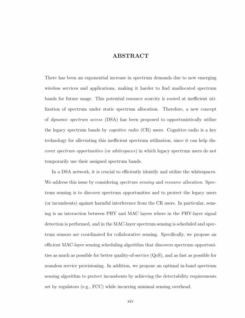
14

3

Ch 1:

Ch 2:

Ch 3:

Logical channel:

time

TIi

Utilized opportunities

Periodic sensing

1

TPi

Sensing overhead:

3 1,3 1 1,3 1 2 1,23 2

Figure 2.1: An example of periodic sensing

this type of sensing is called reactive sensing. On the contrary, a CRN may want to

seek more bandwidth than just staying with a few in-band channels. By discovering

as many in-band channels as possible, the SUs in a CRN may transmit packets at a

higher data rate due to the larger capacity. To discover more idle channels, sensing

is performed proactively even without channel vacation, which is called proactive

sensing. In this chapter, we study proactive sensing with an emphasis on how we

can maximize discovery of opportunities by sensing out-of-band channels. However,

the issues in reactive sensing will be also discussed later in Chapter III.

To discover more idle channels, we consider periodic sensing of out-of-band chan-

nels where each channel has its own sensing-period T iP . Any idle channel discovered

by the periodic sampling becomes a new in-band channel which then can provide

more bandwidth. Although the periodic sensing is performed on every channel in-

dependently, the concurrent sensing of N channels must be scheduled in such a way

that there would be no other scheduled sensing while a measurement on channel

i is being performed for T iI seconds. An example of periodic sensing is shown in

15

Figure 2.1.

In general, more frequent sensing discovers more opportunities. However, one has

to account for the fact that each sensing costs a SU T iI time units without any packet

transmission on the discovered opportunities since there is only a single antenna

for both sensing and transmission. Hence, there is a tradeoff between sensing-time

overhead and discovery of opportunities. In Section 2.4, we propose a sensing-period

optimization for the proactive sensing by making the tradeoff between the discovered

opportunities and the sensing overhead.

The sensing-period optimization approach depends on the underlying channel-

usage patterns which we model as ON-OFF alternating processes. Hence, the key is

to estimate distribution parameters of ON/OFF periods to formulate our objective

functions. Section 2.5 introduces a maximum likelihood (ML) estimation procedure

that can estimate and track time-varying channel parameters.

2.1.1 Contributions

Our contribution in this chapter is two-fold. First, we propose in Section 2.4

an optimal sensing-period mechanism that maximizes the discovered and utilized

amount of spectrum opportunities by considering the tradeoff between discovery of

opportunities and interruption of discovered opportunities. Exploiting the proper-

ties of the renewal process, the optimal sensing-periods are derived for generally-

distributed ON/OFF periods. Second, we introduce in Section 2.5 an ML estimation

technique of the unknown and time-varying channel parameters based on the channel-

state samples produced by sensing. Confidence intervals of the proposed estimators

are also derived and the impact of the length of ON/OFF periods is discussed.

16

2.1.2 Organization

The rest of the chapter is organized as follows. Section 2.2 briefly overviews re-

lated work, and Section 2.3 presents our network model and assumptions. Section 2.4

presents the sensing-period optimization technique to achieve maximum discovery of

opportunities. Section 2.5 introduces the channel-usage pattern estimation method.

The MATLAB-based simulation results are presented and analyzed in Section 2.6.

Example deployment scenarios of the proposed schemes are discussed in Section 2.7.

Finally, we conclude the chapter in Section 2.8.

2.2 Related Work

There have been a limited number of publications on the MAC-layer sensing.

The authors of [14] proposed a proactive sensing algorithm with non-adaptive and

randomly-chosen sensing periods, in which they did not consider how to maximize

discovery of opportunities. [99] proposed a Decentralized Cognitive MAC (DC-MAC)

with reactive sensing focusing on slotted-time CSMA-based channel access with

synchronized slot information. [71] proposed an Ad-hoc Secondary system MAC

(AS-MAC) which is a proactive scheme with slotted-time-based channel access. [99]

and [71], however, did not consider the inherent tradeoff between sensing overhead

and discovery of opportunities. Although [54] pointed out the impact of number

of samples on confidence of estimation, it did not recognize the importance of the

upper-bound approach in adapting sensing-periods as discussed in Section 2.5.

17

2.3 System Model

2.3.1 Network Topology

A group of SUs is assumed to form a single-hop CRN within the transmission

range of which there are no other CRNs interfering or cooperating with that CRN.

In a practical CRN, however, such as an IEEE 802.22 network [1], the interference

among adjacent CRNs should be dealt with in the context of inter-network coordi-

nation of channel sensing and allocation. Although the coordination issue is not the

main focus of this chapter, our proposed scheme can coexist with any coordination

scheme by dynamically adapting the pool of available channels for a CRN in such a

way that those channels are not used simultaneously by other CRNs.

Every SU in the CRN is assumed to be equipped with a single identical antenna

which can be tuned to any combination of N consecutive licensed channels. This

can be done by the Orthogonal Frequency Division Multiplexing (OFDM) technique

with adaptive and selective allocation of OFDM sub-carriers to utilize any subset of

N licensed channels at the same time [14,47,64]. Note that equipping each SU with

more than one antenna might cause severe interference among its antennas, thus

degrading the SU’s performance [49]. We, therefore, focus on SUs, each equipped

with a single antenna. Each SU works as a transceiver as well as a sensor in its CRN.

2.3.2 Channel and Sensing Model

We follow the channel and sensing model introduced in Chapter I. Each sensing

performs signal detection to identify signals from PUs, where energy and feature

detections are two prominent PHY-sensing schemes. It is assumed that all SUs in

a CRN should participate in sensing a channel at the same time for each scheduled

measurement, which is known as collaborative sensing. Collaborative sensing exploits

18

location diversity of multiple nearby sensors and enhances detection performance of

PU signals in terms of mis-detection and false-alarm probabilities [31,34,94] even in

fading/shadowing environments. Since collaborative sensing itself is not our major

focus, we will use a simple collaboration policy of letting all SUs participate in

simultaneously sensing a channel, as a baseline study.

In collaborative sensing, the sample of a channel collected by a SU must be

shared/synchronized with other SUs so that each SU can decide on the channel’s

availability. The authors of [34] introduced a simple rule (OR-rule) in which a channel

is considered ON if at least one SU reports that the channel is busy. Since the

cooperation among SUs is not a focus of this chapter, we assume the sensing-time

T iI includes both PHY-layer detection time (e.g., 1 ms for energy detection [18]) and

data synchronization time in collaborative sensing.

2.3.3 Opportunity-Usage Model

Whenever sensing is performed on a channel and an opportunity on the channel

is discovered, the channel is merged into a pool of available channels where the

pool is called a logical channel. Therefore, a logical channel can include 0 ∼ N

licensed channels depending on their availability at that instant. The logical channel

is treated as if it were a single channel whose capacity is equal to the sum of all

licensed channels merged into it. This can be done by using the OFDM technique

with selective allocation of sub-carriers to the channels to be utilized [14, 47, 64]. In

this way, more than one (possibly non-adjacent) channels in the logical channel can

be simultaneously utilized by SUs.

Return of PUs to an in-band channel should be detected promptly to minimize

interference on them. This can be done by in-band sensing which will be actively

19

discussed in Chapter IV. Hence, we assume returning PUs can be detected within a

reasonably small amount of time so that the channel can be vacated by SUs promptly.

To vacate the channel due to returning PUs, OFDM should reconfigure sub-carriers

to exclude the channel band from usage.

2.4 Maximal Discovery of Opportunities by Optimizing Sensing-Period

When proactive sensing is employed by a CRN and each channel is sensed peri-

odically with its own sensing-period, we would like to optimize the set of N sensing-

periods (T iP ’s) to maximize the discovery of opportunities.

Since sensing is nothing but a sampling process, it is not possible to exactly iden-

tify each state transition between ON and OFF periods. Hence, the time portion of

a discovered OFF period between the start-time and the discovery-time of the OFF

period cannot be utilized. In addition, some OFF periods may remain undiscovered

at all if sensing is infrequent. However, blindly increasing the sensing frequency is

not desirable, as it will increase the sensing overhead, which is proportional to the

sum of (T iI/T

iP ). Note that the sensing overhead is the time-overhead during which

all data traffic among SUs must be suspended to measure a channel’s availability.

This tradeoff must be captured in the construction of an equation to find the opti-

mal sensing frequencies/periods. So, for each channel i we define two mathematical

terms, UOPP i(T iP ) (Unexplored Opportunity) and SSOH i(TP) (Sensing Overhead)

where TP = (T 1P , T 2

P , . . . , TNP ). UOPP i(T i

P ) is defined as the average fraction of time

during which channel i’s opportunities are not discovered, in case the channel i is be-

ing periodically sensed with its sensing-period T iP . On the other hand, SSOH i(TP)

is defined as the average fraction of time during which channel i’s discovered op-

20

Channel 2

Channel 1Sensing on channel 1 & 2

Discovered opportunity

in channel 1

Channel 1’s opportunity

interrupted due to

sensing channel 2

Figure 2.2: The concept of SSOH i: channel 1’s discovered opportunity cannot beutilized during sensing of channel 2

portunities are interrupted and not utilized due to sensing of one of N channels.

An already-discovered opportunity within a channel will be interrupted by sensing

because we assumed: (i) a SU is equipped with a single antenna, and (ii) all SUs

in the CRN must participate in sensing a channel. That is, the SUs must suspend

use of a discovered channel when it senses other channels, since data transmission

and sensing cannot take place at the same time with one antenna. This situation is

depicted in Figure 2.2.

Since ui is defined as the average fraction of time channel i is busy, the average

sum of opportunities per unit time is given as (1 − ui). Our objective function is

then to find optimal sensing-periods of N channels, such that

TP∗ = arg max

TP

{N∑

i=1

{(1− ui)− SSOH i(TP)− UOPP i(T iP )}

}

= arg minTP

{N∑

i=1

{SSOH i(TP) + UOPP i(T iP )}

} (2.1)

where TP∗ = (T 1

P∗, . . . , TN

P∗) is a vector of optimal sensing-periods. As a boundary

condition of T iP ,

N∑i=1

T iI

T iP

< 1 should be satisfied, providing a lower-bound of T iP .

2.4.1 Analysis of UOPP i(T iP )

We define T id(t) (d = 0, 1) as the average of opportunities (measured in time

units) on channel i during (ts, ts + t), provided a sample d is collected at time ts.

21

0 1( ) = ( - )

i iT t x + T t x%% %

(i) (ii)

0( ) =

iT t t

ts

1 ( ) :i

T t (i) (ii)

1 0( ) = ( - )

i iT t T t y% %

ts+ t ts ts+ t

ts ts+ t ts ts+ t

01 ( ) =i

T t

x% x% -t x%

y% y%

0( ) :

iT t

x0 ( ) :i

T t% t - x

0 1( ) = ( - )

i iT t x + T t x% %

(i) (ii)

y

x

0( ) =

iT t t%

ts

1 ( ) :i

T t% (i) (ii)

1 0( ) = ( - )i i

T t T t y% %

y

ts+ t ts ts+ t

ts ts+ t ts ts+ t

01

( ) =iT t%

Figure 2.3: Illustration of T i0(t), T i

1(t), T i0(t) and T i

1(t) - x/y denotes the remainingtime in the current OFF/ON period starting from ts. In case the statetransition occurs at ts, x/y is used instead of x/y.

In case the state transition (ON→OFF or OFF→ON) occurs at ts, T id(t) (instead of

T id(t)) is used to denote the same metric. Possible scenarios of those four functions

T i0(t), T i

1(t), T i0(t) and T i

1(t) are illustrated in Figure 2.3. Note that T id(TP

i) implies

the average amount of channel availability between two consecutive samples in case

the first sample is d.

According to the renewal theory, for an alternating renewal process which has

been started a long time ago, the remaining time x in the current state (say, OFF

22

~ ( )iOFF

i

OFF TT f x

ts

... ( )~ ( )

[ ]

iOFF

iOFF

Ti

OFF iTOFF

xT f x

E T=

%

%% %

x

x%

Figure 2.4: The density function of the remaining time in the current OFF period

state) from the sampling time ts has its p.d.f. of FT iOFF

(x)/E[T iOFF ], x > 0 [20, 68],

where FT iOFF

(x) = 1− FT iOFF

(x) and FT iOFF

(x) is the c.d.f. of the OFF period. This

is illustrated in Figure 2.4, where T iOFF is a random variable of the remaining time

in the OFF period. Similarly, the p.d.f. of the remaining time in ON state from ts is

given as FT iON

(y)/E[T iON ], y > 0.

Since these are asymptotic pdfs, application of the pdfs produces approximate

solutions. However, using the asymptotic pdfs helps us to analyze the problem even

with generally distributed ON/OFF periods, not just for exponentially distributed

ones. The impact of such approximation will be evaluated in Chapter V, where it

will turn out that our approximation technique is very effective to model the general

renewal channels with reasonably small errors.

Using the above facts, we can derive the following equations:

T i0(t) = t

∫ ∞

t

FT iOFF

(x)

E[T iOFF ]

dx +

∫ t

0

FT iOFF

(x)

E[T iOFF ]

(x + T i

1(t− x))

dx,

T i1(t) =

∫ t

0

FT iON

(y)

E(T iON)

T i0(t− y)dy,

T i0(t) = t

∫ ∞

t

fT iOFF

(x)dx +

∫ t

0

fT iOFF

(x)(x + T i

1(t− x))

dx,

T i1(t) =

∫ t

0

fT iON

(y)T i0(t− y)dy.

23

By performing the Laplace transform, we get

T i0

∗(s) = {FXi

∗(0)− FXi∗(s)} /

{E[T i

OFF ] · s2}

+ FXi∗(s)T i∗

1 (s)/E[T iOFF ],

T i1

∗(s) = FT i

ON

∗(s)T i∗0 (s)/E[T i

ON ],

T i∗1 (s) = fT i

ON

∗(s)T i∗0 (s),

T i∗0 (s) =

{fT i

OFF

∗(0)− fT iOFF

∗(s)}

/s2 + fT iOFF

∗(s)T i∗1 (s).

Hence it leads to:

T i∗0 (s) =

1

E[T iOFF ] · s2

·[F∗T i

OFF(0)− F∗T i

OFF(s) ·

1− f ∗T i

OFF(0)f ∗

T iON

(s)

1− f ∗T i

OFF(s)f ∗

T iON

(s)

],

T i∗1 (s) =

F∗T i

ON(s)

E(T iON) · s2

·f ∗

T iOFF

(0)− f ∗T i

OFF(s)

1− f ∗T i

OFF(s)f ∗

T iON

(s).

Now, we develop an expression of UOPP i(T iP ) in terms of T i

0(t) and T i1(t).

1 A

new term UOPP i(d)(T

iP ) is defined as the average fraction of time during which usable

opportunities are not discovered between two consecutive samples in case the first

sample is d. Then, UOPP i(T iP ) = (1− ui) · UOPP i

(0)(TiP ) + ui · UOPP i

(1)(TiP ).2

In case d = 1 is collected at time ts, opportunities existing in (ts, ts + T iP ) cannot

be discovered since there is no more sensing between two sampling times ts and

ts + T iP . Since the amount of opportunities in (ts, ts + T i

P ) is given as T i1(TP

i),

UOPP i(1)(T

iP ) =

[T1(T

iP )

T iP

].

In case d = 0 is collected at time ts, the opportunity discovered at ts starts to be

utilized until PUs’ return. If the OFF period lasts more than T iP after ts, there will

not be any unexplored portion of opportunities in (ts, ts + T iP ). On the contrary, if

PUs emerge at te (ts < te < ts + T iP ), any opportunities in (te, ts + T i

P ) could not be

1Note that T id(t) can be derived from T i

d(t).2Note that a channel is assumed to be in its equilibrium state, and in such a case, ui is the

probability that a sample 1 is collected from channel i at a random time point [20,68].

24

explored since the next sampling time is ts + T iP . Hence,

UOPP i(0)(T

iP ) =

1

T iP

∫ T iP

0

FT iOFF

(x)

E[T iOFF ]

T i1(T

iP − x)dx

which completes the derivation of UOPP i(T iP ).

Two examples of UOPP i(T iP ) are introduced here. In case channel i’s ON/OFF

periods are Erlang-distributed, we have

fT iOFF

(x) = xe−x, fT iON

(y) = ye−y (x, y > 0), (2.2)

UOPP i(T iP ) =

1

2− 3

4T iP

+e−T i

P

4

(3

T iP

+ 1

).

On the other hand, for exponentially-distributed ON/OFF periods, we have

fT iOFF

(x) = λT iOFF

e−λ

TiOFF

x(x > 0), fT i

ON(y) = λT i

ONe−λ

TiON

y(y > 0), (2.3)

UOPP i(T iP ) = (1− ui) ·

{1− 1− e

−λTi

OFFTP

i

λT iOFF

TPi

}.

These results are reasonable in the sense that limTP

i→∞UOPP i(T i

P ) = 1 − ui. As

TPi →∞, no opportunity is discovered since no sensing will be performed. Therefore,

UOPP i(T iP ) becomes (1− ui).

2.4.2 Analysis of SSOH i(TP)

As defined earlier, SSOH i(TP) is the average fraction of time during which

channel i’s discovered opportunities cannot be utilized due to sensing of N channels.

To express SSOH i(TP) mathematically, we introduce a concept of observed channel-

usage pattern. Since a channel’s ON-OFF usage pattern is partially observed by SUs

via sensing at discrete-time points, the exact renewal times (i.e., state transition

times such as ON → OFF or OFF → ON) cannot be observed by SUs. Instead, we

use observed ON-OFF pattern of channel i to derive SSOH i(TP). In the observed

ON-OFF model, a channel’s OFF period starts when the OFF period is discovered.

25

original channel observed channel

Figure 2.5: The observed channel-usage pattern model

Once an OFF period is discovered, however, the next state transition to the following

ON period is assumed to be recognized via the Listen-before-Talk policy. Figure 2.5

illustrates the concept of the new model. This model’s channel utilization is called

modified channel utilization, denoted by ui, which is given as ui = ui +UOPP i(T iP ).

Using the new model, SSOH i(TP) can be derived as

SSOH i(TP) = (1− ui)N∑

j=1

(T j

I

T jP

).

In the above equation of SSOH i(TP), (1 − ui) implies the time fraction in which

channel i’s opportunities are discovered. The reason for using ui instead of ui is

that SSOH i is only concerned with the discovered portion of OFF periods by its

definition. The second termN∑

j=1

(T j

I

T jP

)means the cumulative sensing overhead due to

sensing on N channels.

2.4.3 Sensing-Period Optimization Algorithm

Based on the derived expressions of UOPP i(T iP ) and SSOH i(TP), the optimal

sensing periods can be determined by solving Eq. (2.1).

2.5 Channel-Parameter Estimation

The estimation of the underlying channel-usage patterns is important to the pro-

posed sensing-period optimization approach, since its solution is expressed with the

unknown channel parameters. Therefore, we introduce an ML estimation technique

26

to estimate the time-varying distribution parameters of an ON/OFF alternating re-

newal channel.

2.5.1 Maximum Likelihood (ML) Estimators

Suppose we have a vector of ri samples from channel i, Zi = (Zit1, Z i

t2, . . . , Z i

tri),

where tj (j = 1, . . . , ri) denotes the timestamp of sample Zitj. Suppose the density

functions of ON and OFF periods are m-variate, then a total of 2m parameters

should be estimated. On the other hand, the joint probability mass function of ri

samples can be expressed with 4 types of transition probabilities (0→0, 0→1, 1→0,

1→1) as follows:

θi = (θi1, . . . , θ

i2m),

L(θi) = P (Zi; θi) = Pr(Zit1

= z1; θi) ·

ri∏

k=2

Pr(Zitk

= zk|Zitk−1

= zk−1; θi)

= Pr(Zit1

= z1; θi)

ri∏

k=2

P izk−1zk

(tk − tk−1; θi)

where the Markovian property has been applied. P izk−1zk

(tk − tk−1) denotes the

probability that a sample zk−1 is followed by a sample zk and the inter-sample-

collection time is tk − tk−1. Then, the estimates of parameters of ON/OFF density

functions can be found by maximum likelihood estimation, such as

∂lnL(θi)

∂θil

= 0, l = 1, . . . , 2m.

Now, the remaining task is to express the likelihood function in a mathematical

form. The first component of the likelihood function is given as Pr(Zit1

= z1; θi) =

(ui)z1(1 − ui)1−z1 since ui is the probability that channel i is busy (i.e., ON) at a

random time (t1 in this case). Note that the estimator of ui is simply given as the

sample mean of ri samples.

27

Another part of the likelihood function is P izk−1zk

(tk−tk−1; θi), which is one of four

transition probabilities: P i00(tk−tk−1), P

i01(tk−tk−1), P

i10(tk−tk−1) and P i

11(tk−tk−1).

The renewal theory [20] suggests that P i11(∆), ∆ = tk − tk−1, is expressed as

P i11(∆) =

∫ ∞

∆

FT iON

(u)

E[T iON ]

du +

∫ ∆

0

hi10(u)FT i

ON(∆− u)du (2.4)

where hi10(u) is the renewal density of OFF state given that the renewal process

started from ON state. It is proven in [20] that hi∗10(s) is expressed as

hi∗10(s) =

f ∗T i

OFF(s)

{1− f ∗

T iON

(s)}

E[T iON ] · s

{1− f ∗

T iON

(s)f ∗T i

OFF(s)

} .

By applying the Laplace transform, Eq. (2.4) becomes

P i∗11(s) =

1

s−

{1− f ∗

T iON

(s)}{

1− f ∗T i

OFF(s)

}

E[T iON ] · s2

{1− f ∗

T iON

(s)f ∗T i

OFF(s)

} .

Similarly, P i00(∆) can be easily derived by switching the role of state ON and

OFF such as

P i∗00(s) =

1

s−

{1− f ∗

T iOFF

(s)}{

1− f ∗T i

ON(s)

}

E[T iOFF ] · s2

{1− f ∗

T iOFF

(s)f ∗T i

ON(s)

} .

Finally, P i10(∆) and P i

01(∆) can be derived by using the following relationship:

P i10(∆) = 1− P i

11(∆) and P i01(∆) = 1− P i

00(∆).

For example, for a channel with exponentially-distributed ON/OFF periods as

shown in Eq. (2.3), transition probabilities are given as

P i00(t) = (1− ui) + ui · e−(λ

TiOFF

+λTi

ON)t,

P i01(t) = ui − ui · e−(λ

TiOFF

+λTi

ON)t,

P i11(t) = ui + (1− ui) · e−(λ

TiOFF

+λTi

ON)t,

P i10(t) = (1− ui)− (1− ui) · e−(λ

TiOFF

+λTi

ON)t.

(2.5)

28

Then, there are two parameters to be estimated: λT iOFF

and λT iON

. Since ui =

E[T iON ]

E[T iON ]+E[T i

OFF ]=

λTi

OFF

λTi

ON+λ

TiOFF

, we can estimate λT iOFF

and ui, instead of λT iOFF

and

λT iON

.

As already discussed, the estimator of ui is given as

ui =1

ri

ri∑

k=1

Zitk

.

On the other hand, the estimator of λT iOFF

can be derived by solving the equation

∂lnL(θ)/∂λT iOFF

= 0, yielding

λT iOFF

= − ui

T iP

ln

[−B +√

B2 − 4AC

2A

],

where

A = (ui − (ui)2)(ri − 1),

B = −2A + (ri − 1)− (1− ui)n0 − ui · n3,

C = A− ui · n0 − (1− ui)n3.

Note that n0/n1/n2/n3 indicates the number of 0→0/0→1/1→0/1→1 transitions

from the total of (ri − 1) transitions among ri samples. For instance, in case a

sequence of samples is given as (0,1,1,1,0,1,1,0), ri = 8, we have n0 = 0, n1 = 2, n2 =

2, n3 = 3.

2.5.2 Confidence Interval of Estimators

It is also important to understand how much one can have confidence in the de-

rived estimators. The confidence interval is an efficient measure to determine the

level of confidence. In most cases, however, it is not easy, or sometimes impossi-

ble to derive the confidence interval in a closed form with generally-formed density

functions of ON/OFF periods. Here, we show derivation of confidence intervals with

exponentially-distributed ON/OFF periods.

29

Confidence interval of ui

When channel i is periodically sensed at an interval T iP , the difference between

any two timestamps Ztk1and Ztk2

(k1, k2 ∈ {1, 2, . . . , ri}) is an integer multiple of T iP .

In such a case, the correlation coefficient of any two samples Ztk1and Ztk2

(k1 > k2)

is found to be

E[Ztk1Ztk2

] = Pr(Ztk1= 1|Ztk2

= 1) Pr(Ztk2= 1) = P i

11(|k1 − k2| · T iP ) · ui

⇒ ρk1k2 =E[Ztk1

Ztk2]− (ui)2

ui − (ui)2= e

−(λTi

OFF/ui)·|k1−k2|T i

P .

(2.6)

This shows that the correlation is decaying fast (exponentially) as the separation

of two sampling times becomes large. Since the rate of decrease is proportional to

(λT iOFF

/ui)T iP , ri samples can be assumed to be weakly-correlated as ri are large

unless (λT iOFF

/ui)T iP is close to 0. Using this fact, we can derive the confidence

interval. When (λT iOFF

/ui)T iP is not close to 0, Zi−E[Zi]√

var[Zi]→ N(0, 1) as ri →∞ by the

Central Limit Theorem.3 Hence, 100(1− α)(%) confidence interval is given as

[Zi −

√var[Zi] ·N−1(1− α/2), Zi +

√var[Zi] ·N−1(1− α/2)

].

where var[Zi] is a function of ri. If β ≡√

var[Zi] ·N−1(1 − α/2), ri can be related

to the level α of confidence with the interval length of 2β. In general, we need more

samples (i.e., bigger ri) to achieve a higher level of confidence (i.e., smaller α or β).

Confidence interval of λT iOFF

The ML estimator of λT iOFF

has already shown. Unfortunately, the high non-

linearity of λT iOFF

makes it difficult to find its exact confidence interval. Instead,

an upper bound of T iP could be derived to ensure a reasonable level of confidence.

Note that each of four transition probabilities tends to converge to a constant (ui or

3 Zi is the sample mean of Zi = (Zit1 , Z

it2 , . . . , Z

itri

).

30

0 1 2 3 4 5 6 7 8 9 100

0.05

0.1

0.15

0.2

0.25

0.3

0.35

0.4

u = 0.347826

TP

(sensing period)

P0

1( TP

)

(1 γ ) ⋅ u

upper bound

Figure 2.6: The graph of P i01(T

iP ) and upper bound of T i

P

1−ui), as T iP goes to infinity. Since lnL(θi) is expressed with transition probabilities,

an ML estimator cannot guarantee accurate estimation with a large T iP with which

the likelihood function tends to be a constant. Hence we will bound the value of

P i01(T

iP ) below a certain threshold (1 − γ)ui to ensure the probability would not be

too close to its limit. This concept is shown in Figure 2.6. Then, an upper bound of

T iP can be derived as

|ui − P i01(T

iP )| ≥ γ × ui ⇒ T i

P ≤ui

λT iOFF

ln

(1

γ

).

Hence, the optimal sensing-period in Section 2.4 should be determined subject to

the constraint of the upper bound of T iP given here.

Discussion

We can apply the same intuition derived from the case of exponentially-distributed

ON/OFF periods to general distributions. First, upon estimation of channel utiliza-

tion ui, the more samples are given, the more accurate estimates. On the other hand,

if we want to estimate E[T iOFF ] and E[T i

ON ], it is important to upper-bound T iP so

that a sufficient number of samples would be collected within each OFF/ON period.

31

If T iP increases, both E[T i

OFF ] and E[T iON ] will be over-estimated, as many OFF/ON

periods would be missed by the sensing. So, the number of samples and sensing

frequency are two important factors that control the confidence level of estimation.

2.5.3 Estimation on Time-Varying Channels

The ON-OFF patterns of licensed channels are often time-varying, implying that

the parameter estimation must be adaptive in time. Here we assume that the channel

parameters of ON/OFF periods are slowly time-varying so that the SUs can track

their variations by using a moving time-window in collecting samples and making

estimation. That is, channel i’s sensing results (binary samples) are preserved for

those whose sampling timestamps are no older than T iwindow, where T i

window indicates

the time-window size of channel i. The estimation procedure must be executed

frequently enough to track the variation of parameters. As an extreme case, new

estimates might be produced every time when a new sample is collected from a

channel, although it may incur high processing cost. Therefore, in Section 2.6, we

compute estimates once every Testimation seconds, which is much smaller than T iwindow.

Note that whenever new estimates are computed, the optimal sensing periods derived

in Section 2.4 must be re-calculated and adapted accordingly.

2.6 Performance Evaluation

2.6.1 Simulation Setup

To measure the effectiveness of the proposed schemes, we define a performance

metric called Achieved Opportunity Ratio (AOR). AOR measures the ratio of the

total discovered spectrum availability to the total existing availability. This metric

will show the efficiency of the proposed sensing-period optimization in terms of the

percentage of total opportunities it can discover. Ideally, if all estimates are perfect,

32

AOR will be as high as

AORmax =

N∑i=1

{(1− ui)− SSOH i(T∗

P)− UOPP i(T iP∗)}

N∑i=1

(1− ui)

where the numerator comes from Eq. (2.1). In practice, however, AORmax cannot

be achieved since estimates are not perfect. We will show how much the actual

simulation results deviate from AORmax.

In addition to the above, we also study how close the estimation results would

be to the actual channel-parameters, and how well estimates track time-varying

channels.

We conducted simulation using MATLAB, and all N channels are assumed to

have exponentially-distributed ON/OFF periods. A total of 9 heterogeneous channels

have been used (i = 1, 2, . . . , 9), where (λiTOFF

, λiTON

) are independently chosen. We

tested different channel conditions by changing the number of channels to be sensed

such as: (1) 3 channels (channel 1,2,3), (2) 6 channels (channel 1,2,. . .,6), and (3) 9

channels (channel 1,2,. . .,9). For each case, a simulation ran for 5,000 seconds and

AOR was measured. To observe the average behavior, the simulation under the same

condition was repeated 10 times.

To emulate time-varying channel conditions, the channel parameter λiTOFF

/λiTON

decreases/increases its value by 10% once every 1,000 seconds. This allows us to show

the efficiency of parameter tracking of our estimation with a moving time-window.

The proposed sensing-period optimization scheme is comparatively evaluated

against a reference scheme without sensing-period optimization. Since there is no

sensing-period adaptation in the reference scheme, it starts with a randomly-chosen

initial sensing-period which will not be adapted. The reference scheme is tested

with four different initial T iP : 0.05, 0.1, 0.5, and 1.0 seconds (∀i). For the pro-

33

γ T iwindow (∀i) Testimation T i

I (∀i)0.2 200(sec) 20(sec) 2(ms)

Table 2.1: General evaluation parameters

AOR test Proposed Reference

Initial T iP 0.5(sec) 0.05/0.1/0.5/1.0 (sec)

Table 2.2: AOR test parameters

Ch 1 Ch 2 Ch 3 Ch 4 Ch 5 Ch 6 Ch 7 Ch 8 Ch 9

E[T iOFF ] 1.50 0.50 1.00 3.00 1.00 3.50 4.00 0.50 0.75

E[T iON ] 0.80 2.50 1.00 2.50 2.00 0.50 1.00 5.50 2.00

Table 2.3: Channel-usage pattern parameters

posed scheme, the algorithm starts with the initial T iP of 0.5 (seconds), and is then

adapted and optimized gradually. This comparison will clearly show the importance

of sensing-period optimization to efficient collection of more opportunities.

The parameters used for the simulation are shown in Tables 2.1, 2.2, and 2.3,

where E[T iOFF ] and E[T i

ON ] are in seconds.

2.6.2 The Simulation Results

Achieved Opportunity Ratio

Figure 2.7 plots the AOR of the proposed and reference schemes. The x-axis

represents the number N of licensed channels and y-axis presents AOR in %. 100%

indicates that a scheme can discover/utilize all existing opportunities of∑N

i=1(1−ui),

which is in practice impossible to achieve due to the sensing overhead (SSOH i)

and the missed portion of opportunities (UOPP i). Thus, it is more meaningful to

consider the analytical maximum of utilizable opportunities (AORmax).

The results in the figure show the superiority of the proposed algorithm. The

sensing-period optimization offers more than 98% of the analytical maximum of

34

discovered spectrum availability regardless of the tested conditions (N = 3, 6, or 9).

The small deviation of the performance from AORmax comes from three factors: (1)

the time for estimates to converge to the time-varying parameters, (2) the time for

sensing-periods to be adapted to optimal ones, and (3) small deviation of estimates

from the actual parameters. It also discovers up to 22% more opportunities than the

reference schemes which do not offer sensing-period optimization. This improvement

may become greater as the initial T iP is chosen smaller than 0.05 second, or larger

than 1.0 second. In fact, no reference scheme can outperform the proposed scheme.

As initial T iP is chosen farther away from the optimal one, the performance of the

reference scheme degrades greatly for two reasons. First, if T iP grows, SSOH i gets

smaller but UOPP i becomes larger and dominant, resulting in many missed OFF

periods. In contrast, if T iP decreases, UOPP i gets smaller and more OFF periods are

discovered, but SSOH i becomes larger, resulting in frequent interrupts in utilizing

discovered opportunities on a channel due to sensing channels. Hence, in either case

the reference scheme cannot reach AORmax.

One may claim that in some cases (e.g., initial T iP = 0.1 at N = 3) the reference

scheme nearly achieved AORmax. The reference scheme, however, chooses initial T iP

randomly and does not optimize it. Therefore, it would be just a pure luck if the

reference scheme chooses its initial T iP close to the optimal one. In addition, non-

adaptive T iP cannot track time-varying channel environments and will eventually

yield poor performance if the simulation was run long enough. On the other hand,

the sensing periods in the proposed scheme are adapted to the optimal values in a

few cycles and they also track changing optimal values as shown in Figure 2.8, where

adaptation is performed every Testimation (sec). Dashed lines indicate analytically-

derived target optimal sensing-periods.

35

3 6 90

10

20

30

40

50

60

70

80

90

100

# of channels

Ach

iev

ed O

pp

ort

un

ity

Ra

tio

(%

)

AORmax

Proposed

Reference ( TP

init =0.05)

Reference ( TP

init =0.1)

Reference ( TP

init =0.5)

Reference ( TP

init =1.0)

AORmax

Proposed

Figure 2.7: Achieved opportunity ratio (AOR)

0 500 1000 1500 2000 2500 3000 3500 4000 4500 50000

0.02

0.04

0.06

0.08

0.1

0.12

0.14

0.16

0.18

0.2

Elapsed Simulation Time (sec)

TP (s

ensi

ng-p

erio

d)

Figure 2.8: Adaptation of sensing-periods (N=3 case: channel 1)

Channel-Parameter Estimation Accuracy

Figure 2.9 shows the accuracy of our channel-usage pattern estimation. Each

point in the figure indicates the estimate produced within an estimation cycle,

Testimation. Dashed lines represent the actual target channel parameters. The plot

of ui as well as λT iOFF

follow the actual channel parameters very closely even when

they are time-varying. The difference between estimates and target values can be

36

0 500 1000 1500 2000 2500 3000 3500 4000 4500 50000

0.1

0.2

0.3

0.4

0.5

0.6

0.7

0.8

0.9

1

Elapsed Simulation Time (sec)

u (

cha

nn

el u

tili

zati

on

)

channel 1

channel 2

channel 3

(a) ui

0 500 1000 1500 2000 2500 3000 3500 4000 4500 50000

0.5

1

1.5

2

2.5

3

3.5

4

Elapsed Simulation Time (sec)

λOFF

channel 1

channel 2

channel 3

(b) λiOFF

Figure 2.9: Estimation of unknown channel parameters: N=3 case

controlled by adapting γ and T iwindow, which are related to the number of samples

and confidence intervals of estimators.

2.7 Deployment Scenarios

This section discusses how our proposed schemes can be applied to IEEE 802.11

systems as well as other licensed bands.

37

2.7.1 Application to IEEE 802.11

First, due to limitations in CSMA, 802.11 cannot be directly used as a platform of

the proposed schemes. The Clear Channel Assessment (CCA) in CSMA uses energy

detection to determine if there is any signal activity in each time slot, and hence,

cannot differentiate SU signals from PU signals. As a result, all SUs could be backed

off in case there is a PU signal within a contention period, since every SU may think

the channel is occupied by another SU, not by PUs. It is, however, not desirable

because all SUs have to vacate the channel if there exists any PU.

Hence, the current CCA of 802.11 should be modified in such a way that during

a quiet period, no random back-off or data transmission is performed. In addition,

the measurement result (busy or idle) of every slot during the quiet period must be

reported to the MAC layer, and the MAC should also be modified so that the sensing

results can be distributed to and shared by SUs.

To support periodic sensing scheduling on in-band and out-of-band channels,

802.11 MAC should introduce a new feature to reserve quiet periods. It can be done

by using beacons or regular packets exchanged among SUs.

One example of using the 802.11 platform/protocol to implement sensing func-

tionalities is described in [49] where an incumbent detection mechanism has been

implemented using a commercial WLAN device (Atheros) and its open source de-

vice driver, MadWifi. In terms of sensing-periods, a in-band channel is regularly

monitored once every frame (100 ms) to detect returning PUs (emulated by a signal

generator emitting signals on one of WiFi bands). The sensing-period adaptation,

however, can also be implemented by reserving a quiet period (at MAC level) every

n frames and adapting n accordingly.

38

2.7.2 Application to licensed bands

The proposed sensing-period optimization scheme is designed to be adaptive to

time-varying channel environments in order to track diverse channel-usage behavior

of heterogeneous applications (e.g., voice, video streaming, web browsing, etc.). For

example, if there exists a long ON period on a TV band, the proposed adaptive

estimation technique with a moving time-window will accumulate 1 (ON) samples

and its estimates of mean ON/OFF periods will eventually converge to the max-

imum/minimum values. As a result, the channel’s sensing-period is adapted to a

larger value since the channel is not likely to be available.

In case a licensed band has very short ON/OFF periods, spectrum agility may

not bring much benefit due to high sensing overhead to track the fast ON/OFF

state transitions. Our goal in this chapter, however, is to provide a general sensing

framework which can be applied to any application on any band, by providing an

adaptive sensing method and estimation technique.

2.8 Conclusion

In this chapter, we have proposed a sensing-period adaptation scheme used to

discover spectrum opportunities more efficiently. The proposed scheme strives to dis-

cover as many utilizable spectrum opportunities as possible. Channel-usage pattern

estimation was also proposed by deriving ML estimators and their confidence inter-

vals. The simulation results demonstrated the advantages of the proposed schemes,

such as a larger amount of discovered opportunities and robust parameter estima-

tion.

39

CHAPTER III

OUT-OF-BAND SENSING PART II: FAST

DISCOVERY OF SPECTRUM

OPPORTUNITIES

3.1 Introduction

Opportunity discovery is an act of sensing out-of-band channels to locate an

enough amount of whitespaces to meet the total spectrum demand of a cognitive

radio network (CRN), which may be achieved by a few high-capacity idle channels

or by many low-capacity idle channels by combining their capacities. In this chap-

ter, we consider opportunity discovery in multi-channel CR communications where a

CRN can simultaneously utilize multiple (idle) in-band channels. In such a scenario,

opportunity discovery is triggered when the CRN experiences a shortage of whites-

paces due to the return of primary users (PUs) at one of the in-band channels. The

appearance of PUs incurs channel vacation which, in turn, reduces the amount of

whitespaces the CRN can utilize. Note that the return of PUs is detected by in-band

sensing [51], which will be discussed in Chapter IV.

Fast opportunity discovery is essential to seamless service provisioning for the

secondary users (SUs) in a CRN, because the CRN may not provide its service in full

strength while it experiences a shortage of bandwidth and the discovery of additional

40

opportunities incurs a non-trivial delay. Therefore, it is desired to derive an optimal

way of searching out-of-band channels that minimizes the delay in discovering a

necessary amount of additional bandwidth via out-of-band sensing.

3.1.1 Contributions

Our contribution in this chapter is three-fold. First, we propose an optimal

sensing sequence that minimizes the latency of discovering available out-of-band

channels to achieve the target amount of opportunities. We consider heterogeneous

channel characteristics in terms of signal detection time, channel capacity, and the

probability θi that a channel to be idle, and discuss the difference between offline

and online sequences to show that the optimal sequence is an online sequence. Then,

we derive the optimal online sequence using dynamic programming (DP), and show

that the optimal sequence takes a simple form when channels have homogeneous

capacities. To overcome the computational complexity of the DP algorithm, we also

propose a suboptimal sequence algorithm that shows a near-optimal performance

while incurring insignificant overhead.

Next, we categorize out-of-band channels as backup or candidate channels, as

introduced in IEEE 802.22 [1]. To promote faster discovery of idle channels, we

sort and search backup channels at the time of opportunity discovery where the

backup channels are specially chosen among those that are more probable to have

whitespaces; out-of-band channels other than backup channels are called candidate

channels, and they are not sensed until they are designated as backup channels. Using

this concept, we propose an efficient mechanism that constructs a backup channel

list (BCL) and dynamically updates its entries. The proposed scheme maintains a

moderate size of the BCL and updates its entries by importing/exporting channels

41

from/to the candidate channel list (CCL) with a small computational overhead.

Finally, we propose a strategy that estimates ON/OFF channel-usage patterns

to predict channel availability, by selectively applying ML and Bayesian estimation.

We capture the tradeoff between two estimation techniques: the former is simple but

its performance degrades greatly with infrequent samples; the latter requires more

computation but performs better with a small number of samples [4]. In addition,

our scheme considers imperfect sensing with nonzero probabilities of miss detection

(PMD) and false alarms (PFA) in predicting θi.

3.1.2 Organization

The rest of the chapter is organized as follows. We first overview related work

in Section 3.2, and introduce our system models and assumptions in Section 3.3.

Section 3.4 describes the opportunity discovery mechanism via sequential sensing.

In Section 3.5, we derive the optimal sensing-sequence and a suboptimal sensing-

sequence that achieves a near-optimal performance with small computational over-

head. Section 3.6 presents construction of the initial BCL and an BCL-update al-

gorithm to keep the list up-to-date. Section 3.7 introduces a strategy to estimate

ON/OFF channel-usage patterns using ML and Bayesian inference. The performance

of the proposed schemes are evaluated in Section 3.8, and then the chapter concludes

in Section 3.9.

3.2 Related Work

Among a number of studies on spectrum sensing, several notable bodies of work

are found to be related to fast opportunity discovery. Chang and Liu [9] proposed

a strategy that optimally determines which channel to probe and when to transmit,

but they focused on the case of single channel transmission only. Kim and Shin

42

[50] introduced a sensing-sequence that sorts channels in descending order of the

probability θi, which we call a probabilistic sequence. However, such a sequence only

maximizes the chance of finding an idle channel, instead of minimizing the overall

discovery-delay. Jiang et al. [45] investigated the optimal sensing sequence in a

multi-channel cognitive MAC protocol, and Shu and Krunz [81] studied the problem

of sequential sensing for throughput efficiency along with finding the optimal sensing

time, but both work focused on the case of single channel transmission and identical

sensing time over all channels. In contrast, this chapter considers the case where

CR-to-CR transmission occurs on a multi-channel environment via channel bonding,

and also takes account for heterogeneous channel characteristics with different sensing

times and channel capacities. On the other hand, Ahmad et al. [2] derived an optimal

myopic policy in finding the best channel to sense per each time slot, but their

approach was limited to the single channel sensing per slot and thus different from

our multi-channel sequencing problem. Lai et al. [53] considered a scenario in which

SUs can sense more than one channel simultaneously and utilize all discovered idle

channels for their transmission, but the problem is not based on the specific target

amount of bandwidth to discover as in our case.

On the other hand, Motamedi and Bahai [57] used Bayesian learning to predict

the availability of a channel, where the learning process is simplified by assuming a

geometric distribution for channel-usage patterns. In this chapter, we use a general

alternating renewal process and develop a multi-stage iterative Bayesian inference.

43

3.3 System Model

3.3.1 Network Model

In this chapter, we focus on a single-hop CRN with a central controller (e.g., an

Access Point) and a group of SUs (i.e., CR end-terminals) where the CRN utilizes a

set of M licensed channels from which it harvests the necessary amount of spectrum

opportunities. The M licensed channels are assumed to be determined and given

a priori through an inter-CRN coexistence mechanism such as IEEE SCC 41 [96]

and the coordinated channel allocation schemes [15,60]. The inter-CRN coexistence

scheme coordinates resource allocation between neighboring CRNs which is necessary

to avoid collision by simultaneous channel access, through which the licensed channels

can be assigned to the CRNs in a non-overlapping fashion. Since such schemes are

beyond the scope of this chapter, we focus on selecting backup channels from the

given M channels and optimally sequencing them at opportunity discovery.

Each SU is assumed to have been equipped with a single antenna, widely-tunable

to any combination of M channels. That is, a SU can utilize possibly non-contiguous

multiple idle channels at the same time, which is made possible by using signal

processing techniques such as NC-OFDM [64]. Having one antenna per SU may help

reduce the size of a secondary device and avoid potential interference between co-

located antennas due to their close proximity [49]. A SU is assumed to act as either

a spectrum sensor or a secondary transceiver, by dynamically reconfiguring itself.

We assume the central controller coordinates inter-SU transmission, spectrum

sensing, and channel switching. The SU coordination is performed by a CR MAC

protocol such as C-MAC [19] and OS-MAC [39], which is beyond the scope of this

paper. Using the proposed sensing sequence in Section 3.5, the controller can assign

as many SUs/sensors as necessary to achieve the PU protection requirements (e.g.,

44

PMD and PFA). Note that the optimality of the proposed sensing sequences is intact

regardless of which MAC protocol is employed.

3.3.2 Channel and Sensing Model

We follow the channel model introduced in Chapter I. We also assume channel

i has a capacity of Ci which is a physical bandwidth or Shannon capacity, taken

as a long-term average considering time-varying channel conditions (e.g., fading).

Although instantaneous capacity can also be used in view of fast fading statistics

at each instant, we avoid using such fast-changing channel conditions in achieving

the target amount of opportunities because we do not want overly-sensitive channel

switching due to the short-term degradation of channel quality.

In addition, we use the sensing model introduced in Chapter I. When a SU acts

as a spectrum sensor, it monitors channel i during sensing-time T iI , and determines

the channel state between ON and OFF. T iI is assumed small relative to E[T i

OFF ]

and E[T iON ] such that channel i’s state remains unchanged during the sensing-time.

The value of T iI is determined by the underlying detection method (e.g., energy or

feature detection) and the type of PU signals [18], and thus it varies with channels.

3.3.3 Notation Table

We summarize the frequently used notations in Table 3.1.

3.4 Sequential Sensing Mechanism

In this section, we overview the sequential sensing mechanism for opportunity

discovery, to enhance the understanding of our proposed schemes in the later sections.

45

M number of licensed channels

N number of backup channels (N ≤ M)

i channel index

Zi(t) ∈ {0, 1} channel state at time t (0:OFF, 1:ON)

ui ∈ [0, 1] channel utilization factor

T iI sensing-time

Ci channel capacity

θi channel idle probability at opportunity discovery

Table 3.1: Summary of notations

3.4.1 Opportunity Discovery Procedure

Let Breq denote the total amount of bandwidth a CRN requires, which is the sum

of spectrum demands of all SUs in the CRN. Breq may be achieved by utilizing just

one idle channel with Ci ≥ Breq or by simultaneously utilizing multiple idle channels

whose combined capacity exceeds Breq. Therefore, there exist one or more in-band

channels the CRN currently utilizes.

Opportunity discovery is triggered whenever one of the in-band channels has to

be vacated due to the returning PUs. At opportunity discovery, the CRN needs to

find a set of new idle channels whose collective capacity achieves Btarget, which is

given as

Btarget = max {Breq −Bin−band, 0} ,

where Bin−band is the sum capacity of the remaining in-band channels after the chan-

nel vacation.

New idle channels are discovered by sequentially sensing backup channels such

that SUs synchronously tune to one backup channel at a time following a given

sensing-sequence. Once a backup channel is detected idle, it becomes an in-band

46

ON (busy)

OFF (idle)Ch 1

Ch 2

Ch 3

channel vacation utilized whitespaces

Ch 4

sensing discovery delay

Figure 3.1: An illustration of opportunity discovery when a CRN requires two idlechannels for its operation.

channel and merged into the “logical” channel whose capacity equals the combined

capacity of all in-band channels. Opportunity discovery completes when the logical

channel’s capacity reaches or exceeds Breq. Note that the concept of logical channel

is introduced to help the CRN’s central controller instantly see how much more

bandwidth is required at each channel vacation.

Fig. 3.1 shows an example where all four channels have the same capacity and

the CRN requires two idle channels to meet its Breq. In the figure, the delay of

each opportunity discovery is also shown, which is the sum of sensing-times spent to

sequentially sense the backup channels until Breq is achieved by the newly found idle

channel. Although in this example it suffices to find just one more idle channel per

discovery, we will consider more general cases in the next section where achieving

Breq may require to find more than one idle channel.

Discussion

This chapter focuses on the sequential sensing of backup channels assuming that

all SUs in the CRN participate in sensing an out-of-band channel at each sensing. In

47

reality, however, the CRN may be able to sense more than one channel simultane-

ously if it has a sufficient number of SUs in its network. Since each sensing requires

participation of 10–20 collaborative sensors to enhance the performance of detecting

PUs by exploiting location diversity [31,34,56], the number of backup channels that

can be simultaneously sensed depends on the total number of terminals in the CRN.

For example, if we have 20 SUs and need 10 sensors per channel for collaborative

sensing, then we can sense two channels at the same time. Even in such a case,

however, the sequential sensing still plays a significant role in minimizing the oppor-

tunity discovery delay, since we can first optimally sort all channels and group them

according to the number of channels that can be sensed at the same time.

3.4.2 Channel Idle Probability Prediction

In this chapter, we characterize a channel by a tuple of {T iI , Ci, θi} where T i

I is the

sensing-time, Ci the channel capacity, and θi the probability that channel i would

be idle if the channel is sensed at opportunity discovery. Although derivation of θi

for alternating renewal channels is described in Chapter II, we briefly overview the

procedure here for completeness of the presentation.

θi varies with channels and time since it depends on the ON/OFF usage pattern

and the history of sensing results (or samples). Therefore, calculation of θi first

requires estimation of channel parameters. In Chapter II, an ML estimator and its

confidence interval was derived when a set of samples from channel i is given as

Zi = (Zi(t1), Zi(t2), . . . , Z

i(tr)) where t1 < t2 < . . . < tr. The r samples can be

collected at any time, i.e., they are not necessarily periodic, since they are produced

by (1) sequential sensing at opportunity discovery (if the channel is selected and

sensed), and/or (2) extra sampling scheduled by the central controller who assigns

48

some idle SUs (i.e., SUs with no transmission) to sense out-of-band channels (even

when no opportunity discovery is necessary). The extra sampling is to enhance the

accuracy of estimation but is outside of the scope of this chapter.

Then, Chapter II showed that having t as the opportunity discovery time, θi of

the renewal processes is given as

θi =Pr(Zi(t) = 0|Zi(t1), . . . , Zi(tr)) = Pr(Zi(t) = 0|Zi(tr))

where Pr(Zi(t) = 0|Zi(tr)) is the transition probability between the most recent

sample at time tr and an imaginary sample 0 at time t. The transition probability

is expressed with the estimated channel parameters. For example, exponentially-

distributed ON/OFF periods lead to the following

θi =

(1− ui) + ui · e−(ψiOFF +ψi

ON )(t−tr), if Zi(tr) = 0,

(1− ui){

1− e−(ψiOFF +ψi

ON )(t−tr)}

, otherwise,

which correspond to P i00(t− tr) and P i

10(t− tr) in Eq. (2.5) in Chapter II. Here, two

channel parameters ψiON and ψi

OFF are from

fT iOFF

(t) =ψiOFF e−ψi

OFF t,

fT iON

(t) =ψiONe−ψi

ON t,

(3.1)

where E[T iON ] = 1/ψi

ON and E[T iOFF ] = 1/ψi

OFF .

One can notice that θi 6= (1 − ui) since ui is a long-term average utilization

of channel i while θi is the instantaneous channel idle probability considering the

past channel samples. This also implies that θi reflects the correlation between the

samples. For example, if Zi(tr) = 0 and (t− tr) is small, it is likely that the channel

is still in its OFF state, thus making θi very close to 1. On the contrary, if Zi(tr) = 1

and (t− tr) is small, it is likely that the channel is still in its ON state, thus making

49

θi very close to 0. In addition, once a channel with a long ON period enters the ON

state, the channel’s θi becomes very small until enough time passes.

Sensing Error Compensation

Although the derivation of θi is exact, its correctness relies on how accurately

the samples reflect the actual channel state. In reality, spectrum sensing is imperfect

since PMD and PFA are nonzero. Since the impact of imperfect sensing on θi was

not considered in Chapter II, we introduce here Bayesian state estimation that can

compensate for the sensing error [82]. For the ease of notation, we will omit i in this

subsection.

Suppose Z(tk) ∈ {0, 1} denotes the actual state of a channel at time tk. Assuming

the pdf of the initial state Z(t0) is known, the estimator is

f(Z(t0)|Z0) = f(Z(t0)),

where Zk = {Z(t1), Z(t2), . . . , Z(tk)} for k ≥ 1 and Z0 = ∅. For each k ≥ 1, we

evaluate

f(Z(tk)|Zk−1) =∑

Z(tk−1)

f(Z(tk)|Z(tk−1))f(Z(tk−1)|Zk−1),

f(Z(tk)|Zk) =f(Z(tk)|Z(tk))f(Z(tk)|Zk−1)∑

Z(tk) f(Z(tk)|Z(tk))f(Z(tk)|Zk−1),

where f(Z(tk)|Zk−1) is the prior pmf of Z(tk) before observing Z(tk) and f(Z(tk)|Zk)

is the posterior pmf of Z(tk) after observing Z(tk).

Prior and posterior pmfs are updated whenever a new sample Z(tk) is obtained.

Then, when opportunity discovery is triggered at time t, θ can be estimated as

θ = f(Z(tk)|Zk−1)∣∣∣tk=t,Z(tk)=0

.

50

In the above procedure, f(Z(tk)|Z(tk−1)) and f(Z(tk)|Z(tk)) are yet to be de-

termined. f(Z(tk)|Z(tk−1)) is the transition probability between two consecutive

samples at times tk−1 and tk, which has been fully derived in Chapter II. On the

other hand, f(Z(tk)|Z(tk)) is easily determined according to the definition of PMD

and PFA such as

f(Z(tk)|Z(tk)) =

1− PFA, if (Z(tk), Z(tk)) = (0, 0),

PFA, if (Z(tk), Z(tk)) = (0, 1),

1− PMD, if (Z(tk), Z(tk)) = (1, 0),

PMD, if (Z(tk), Z(tk)) = (1, 1).

3.5 Optimal Sensing Sequence for Minimal Opportunity-DiscoveryLatency

In this section, we derive an optimal sensing-sequence of backup channels that

incurs the minimal delay in discovering a necessary amount of opportunities, and

propose a computationally-efficient sequence algorithm that provides a near-optimal

performance. As introduced in Section 3.4, backup channels are characterized by a

tuple of {T iI , Ci, θi} and the opportunity discovery is triggered at channel vacation

of an in-band channels where the target amount of bandwidth to discover is denoted

by Btarget. For the notational ease, we will use B to denote Btarget throughout this

section.

3.5.1 Problem Statement

Suppose there are N (≤ M) backup channels, and let S = {s1, s2, . . . , sN} ∈ S

be an ordered list of N channels where sj is the channel index of the j-th channel

in the sequence (sj: positive integer, 1 ≤ sj ≤ N) and S is the set of all possible

51

channel-sequences (|S| = N !). Also suppose T iI , Ci and θi are known a priori.

Our objective is to determine the optimal sensing-sequence S∗ that minimizes the

average delay in finding idle channels whose cumulative capacity exceeds B. This

can be stated formally as:

Find S∗ = argminS∈S

Eθ

[N∑

i=1

T siI · I{∑i−1

j=1 Csj ·(1−Zsj )<B}]

where

θ = (θ1, θ2, . . . , θN),

I{?} =

1, if the statement ? is true,

0, otherwise.

(3.2)

In the above problem statement, the indicator function I{∑i−1j=1 Csj ·(1−Zsj )<B} implies

that once B is achieved, the sequential sensing stops.1

3.5.2 Offline vs. Online Sensing Sequences

To find the optimal sensing sequence, we need to consider two types of sensing

sequence: offline and online sequences. In what follows, we will introduce the con-

cept of the two sequences and discuss the reason why the online sequence must be

considered to find the optimal sensing sequence.

Offline Sequence

An offline sensing sequence is a static sequence which strictly follows the initially

determined sequence regardless of the channel states observed during the sequential

1In practice, θ must be updated after sensing each channel by re-calculating θi’s based on theelapsed time due to sensing of the last chosen channel. Although updating θ is always possibleby following the procedure in [50], here we assume T i

I ’s are small enough to make the impact ofadjusting θi’s negligible, for the purpose of easier illustration. In fact, this assumption is applicablein most practical scenarios because T i

I is usually in the order of milliseconds (or even less) whilethe ON/OFF periods are typically in the order of seconds or minutes.

52

sensing. The optimal offline sensing sequence is built by considering θ while ignoring

the actual channel states to be observed, and the average discovery delay D of a given

offline sequence S = {s1, s2, . . . , sN} is given as

D =1∑

z1=0

1∑z2=0

. . .

1∑zN=0

{N∏

v=1

(θsv)1−zv(1− θsv)

zv

×(

T s1I +

N∑v=2

T svI · I{∑v−1

w=1 Csw (1−zw)<B}

)}. (3.3)

Then, the optimal offline sequence is determined as the sequence that minimizes

Eq. (3.3) among N ! possible sequences.

As an example, let us consider the following scenario:

N = 3, B = 2.0, (C1, C2, C3) = (0.5, 1.5, 2.0),

(T 1I , T 2

I , T 3I ) = (1, 2, 3), (θ1, θ2, θ3) = (0.5, 0.3, 0.1). (3.4)

By defining θsj:= 1− θsj

, Eq. (3.3) becomes

D = θs1 θs2 θs3(Ts1I + T s2

I + T s3I ) (3.5)

+ θs1 θs2θs3(Ts1I + T s2

I + T s3I )

+ θs1θs2 θs3(Ts1I + T s2

I + T s3I · I{Cs2<B})

+ θs1θs2θs3(Ts1I + T s2

I + T s3I · I{Cs2<B})

+ θs1 θs2 θs3(Ts1I + T s2

I · I{Cs1<B} + T s3I · I{Cs1<B})

+ θs1 θs2θs3(Ts1I + T s2

I · I{Cs1<B} + T s3I · I{Cs1<B})

+ θs1θs2 θs3(Ts1I + T s2

I · I{Cs1<B} + T s3I · I{Cs1+Cs2<B})

+ θs1θs2θs3(Ts1I + T s2

I · I{Cs1<B} + T s3I · I{Cs1+Cs2<B}).

Then, by comparing all 3! sequences, the optimal offline sequence that minimizes

Eq. (3.5) is found to be {1, 2, 3}.

53

Online Sequence

An online sensing sequence, on the other hand, is a dynamic sequence which can

update itself each time it sense a channel in the sequence such that the remaining

unsensed channels are re-ordered to form an updated sub-sequence according to the

observed channel states. Such a dynamic sequence is necessary to derive the optimal

sensing sequence since the optimality condition changes whenever we sense a new

channel and observe its actual state.

To show the impact of online observation of channel states, let us consider again

the example in Eq. (3.4). Once the first channel in the optimal offline sequence (i.e.,

channel 1) is sensed, the capacity-to-go (i.e., the remaining capacity to achieve at

the subsequent sensing) is updated as

B′ =

B − Cs1 , if channel 1 is sensed idle,

B, otherwise.

(3.6)

Then, we need to find the best channel to sense next to minimize the subsequent

sensing delay D′ in sensing S ′ = {s2, s3}, where

D′ = θs2 θs3(Ts2I + T s3

I ) + θs2θs3(Ts2I + T s3

I )

+ θs2 θs3(Ts2I + T s3

I · I{Cs2<B′}) + θs2θs3(Ts2I + T s3

I · I{Cs2<B′}).

Using B′ and D′ and comparing all (N − 1)! possible subsequences, it can be seen

that the optimal choice of s2 minimizing D′ is given as

s2 =

2, if channel 1 is sensed idle,

3, otherwise.

Therefore, the optimal offline sequence {1, 2, 3} is no longer optimal if the first chan-

nel is sensed busy. Intuitively speaking, when channel 1 is idle, we have B′ = 1.5

54

and thus, we may still want to sense channel 2 next since C2 = 1.5 is large enough to

fulfill B′. When channel 1 is busy, however, we have B′ = 2.0 and we may want to

sense channel 3 instead since channel 2 cannot fulfill B′ while channel 3 can (since

C3 = 2.0). That is, if s2 = 2, the subsequent delay always becomes (T 2I + T 3

I ) re-

gardless of the state of channel 2, whereas the delay might become T 3I if s2 = 3 and

channel 3 is sensed idle.

3.5.3 Optimal Online Sensing Sequence Algorithm

As shown in Section 3.5.2, we need to find the optimal online sequence to mini-

mize the opportunity discovery delay. To find the optimal online sequence, we pro-

pose a dynamic-programming-based search algorithm. We will also show the optimal

sequence takes a simple form for the special case of homogeneous channel capacities.

Let us define an N -stage decision problem where at stage k we have (N − k + 1)

channels to choose from and (k − 1) channels already sensed. Our objective is then,

at stage k, to make an optimal decision on which channel to sense next, to minimize

the overall delay in achieving the target amount of bandwidth, based on the already-

discovered idle channels. For this, we define control uk as the chosen channel to sense

at stage k. We also define xk = (Uk, Bk) as the state at stage k where Uk is the set of

remaining channels to choose from and Bk is the accumulated bandwidth achieved

from the idle channels among the already-sensed. Finally, we define gk(xk, uk) as the

cost incurred at stage k by the chosen control uk, which is in fact the sensing time

T ukI of the chosen channel uk because our goal is to minimize the overall sensing time.

55

B := the total amount of bandwidth to discover;

U1 := {1, 2, . . . , N};B1 := 0;

k := 1;

For all possible combinations of xN = (UN , BN),

derive JN(xN) and uN(xN) by Eq. (3.7);

Using JN(xN), derive all preceding Jk(xk) and uk(xk)

according to Eq. (3.7), for k = N − 1, N − 2, . . . , 1;

while (k ≤ N) {S∗k := uk(xk);

Sensing sequence S∗ := {S∗1 , S∗2 , . . . , S∗k};Sense S∗k and discover its channel state Z;

if (Z == 0) then

Bk+1 := Bk + CS∗k ;

else Bk+1 := Bk;

if (Bk+1 ≥ B) then

Stop the sequential sensing;

return;

Uk+1 := Uk \ {S∗k};k := k + 1;

}return;

Figure 3.2: Pseudo-code of the dynamic programming (DP) search algorithm (S∗:optimal sequence)

Now, the DP algorithm for the optimal online sequence is formulated as follows.

JN(xN) =gN(xN),

Jk(xk) = minuk∈Uk

{Eθ[gk(xk, uk) + Jk+1(xk+1)]},

uk(xk) =arg minu∈Uk{Eθ[gk(xk, u) + Jk+1(xk+1)]},

(3.7)

56

where

gk(xk, uk) = T ukI · I{Bk<B}.

Eq. (3.7) can be further analyzed using the following relationship,

Uk+1 =Uk \ {uk},

Bk+1 =

Bk + Cuk, if channel uk is idle,

Bk, otherwise,

(3.8)

such as

Jk(xk) = minuk∈Uk

{T ukI · IBk<B + θuk

· Jk+1(Uk+1, Bk + Cuk) + (1− θuk

) · Jk+1(Uk+1, Bk)}.

As an initial condition, we have

U1 = {1, 2, . . . , N}, B1 = 0.

Fig. 3.2 presents the pseudo-code of the proposed DP algorithm.

Algorithm Complexity Analysis

Once JN(xN) is computed for every possible xN ’s, Jk(xk) for k ≤ N − 1 can

be iteratively derived. Therefore, the complexity of the algorithm depends on the

number of possible combinations of UN and BN . Since UN is a set of a single element,

there are N possible choices of UN . For a given UN , BN is determined by considering

all possible combinations of the channel states (i.e., idle or busy) of the preceding

N−1 channels—that is, 2N−1. As a result, there are N ·2N−1 possible choices of xN =

(UN , BN) which gives us the complexity of O(N · 2N), and hence the DP algorithm

is not a polynomial-time solution. In Section 3.5.4, we propose a computationally-

efficient suboptimal algorithm that yields a near-optimal performance.

57

A Special Case: Homogeneous Channel Capacity

In this section, we will prove that in a special case with homogeneous channel

capacities, i.e., Ci = C, ∀i, the optimal online sensing-sequence takes a much simpler

form. In Lemma 3.5.1, we first prove that the optimal offline sensing-sequence takes

a trivial form with Ci = C, and then in Theorem 3.5.1 we prove that the optimal

offline sequence becomes the optimal online sequence under the same condition.

Lemma 3.5.1. If Ci = C, ∀i, then the optimal offline sensing-sequence is built by

sorting channels in ascending order of T iI/θi.

Proof. Let L be the optimal sensing-sequence and L′ be its counterpart constructed

by switching the order of the k-th and (k + 1)-th channels in L. That is,

L = (l1, . . . , lk−1, lk, lk+1, lk+2, . . . , lN),

L′ = (l1, . . . , lk−1, lk+1, lk, lk+2, . . . , lN).

On the other hand, DBL is defined as the average delay in locating idle channels

whose cumulative capacity exceeds B, using a sensing-sequence L. PBL is defined as

the probability that the sum of capacities of idle channels in a sensing-sequence L

may be strictly less than B.

In addition, let us define the following ordered lists:

Lk−1 = (l1, l2, . . . , lk−1),

Lk = (l1, l2, . . . , lk),

Lk+1 = (l1, l2, . . . , lk+1),

Lk−1,k+1 = (l1, l2, . . . , lk−1, lk+1),

Lk−1,k+1,k = (l1, l2, . . . , lk−1, lk+1, lk),

Lck+1 = (lk+2, . . . , lN).

58

Since a channel is sensed only when those channels preceding in the list provide

less opportunities than B, we can express DBL and DB

L′ as

DBL = DB

Lk−1+ PB

Lk−1· T lk

I + PBLk· T lk+1

I + PBLk+1

· DBLc

k+1,

DBL′ = DB

Lk−1+ PB

Lk−1· T lk+1

I + PBLk−1,k+1

· T lkI + PB

Lk−1,k+1,k· DB

Lck+1

.

Since DBL ≤ DB

L′ and PBLk+1

= PBLk−1,k+1,k

, we have

PBLk−1

· T lkI + PB

Lk· T lk+1

I ≤ PBLk−1

· T lk+1

I + PBLk−1,k+1

· T lkI

which reduces to

T lkI

(PBLk−1

− PB−ClkLk−1

)θlk

≤ Tlk+1

I

(PBLk−1

− PB−Clk+1

Lk−1)θlk+1

, (3.9)

since PBLk

= PBLk−1

· (1− θlk) + PB−ClkLk−1

· θlk .

By substituting C for Clk and Clk+1in Eq. (3.9), the inequality condition reduces

to:

T lkI

θlk

≤ Tlk+1

I

θlk+1

, for 1 ≤ k ≤ N − 1, (3.10)

which is a necessary condition for optimality. However, since there exists a single and

unique sequence satisfying such a necessary condition,2 the condition also becomes

sufficient. Therefore, the resulting sequence is optimal.

Now, using Lemma 3.5.1, we present the following theorem on the optimal online

sensing sequence.

Theorem 3.5.1. If Ci = C, ∀i, then the optimal online sensing sequence is built

in the same way as the optimal offline sensing sequence, by sorting channels in

ascending order of T iI/θi.

2Note that since θi ∈ [0, 1], it is not likely to have ties with the same T iI/θi. If it happens, we

can still sort them uniquely in ascending/descending order of channel index i.

59

Proof. The optimal online sequence is built by repeatedly searching for the opti-

mal offline subsequences. Let us denote by S the optimal offline sequence of all N

channels. According to Lemma 3.5.1, S is simply constructed by sorting channels

in ascending order of T iI/θi. Then, the first channel in S, say s, becomes the first

channel in the optimal online sequence. Now, to find the next channel in the optimal

online sequence, we need to sort S \{s}, again, according to Lemma 3.5.1. However,

since Eq. (3.10) does not depend on B, the sorted sequence of S \ {s} is still the

same as S \ {s}. Therefore, the second channel in the optimal online sequence is the

second entry of S. By the same argument, S becomes the optimal online sequence,

which proves the theorem.

3.5.4 Efficient Suboptimal Sensing Sequence Algorithm

The proposed DP algorithm suffers from high computational complexity. There-

fore, we propose a computationally efficient algorithm that determines a suboptimal

sequence in polynomial time while providing a near-optimal performance.

To derive a suboptimal sequence, we utilize the necessary condition for optimality

in Eq. (3.9). We first recognize that the first channel in the sequence (i.e., k = 1)

satisfies Lk−1 = ∅, and thus we have PBLk−1

= 1 and

PB−ClkLk−1

=

0, if Clk ≥ B,

1, otherwise,

by the definition of PBL .3 Then, we get

T lkI

(PBLk−1

− PB−ClkLk−1

)θlk

=

T lkI /θlk , if Clk ≥ B,

∞, otherwise.

3Note that the sum capacity of idle channels in an empty set is equal to zero.

60

Therefore, to satisfy Eq. (3.9), the first channel should be the one with the small-

est T iI/θi among all unsensed channels satisfying Ci ≥ B. In case all unsensed

channels have Ci < B, we have PB−ClkLk−1

= 1, and thus the term PBLk−1

− PB−ClkLk−1

in

Eq. (3.9) cancels out. As a result, the first channel in this case (i.e., Ci < B for all

unsensed channels) is determined as the one with the smallest T iI/θi.

Once the first channel is determined, we sense the channel and observe its channel

state. Depending on the state, we update B as in Eq. (3.6) and find the next

channel to sense. Since the problem becomes identical to the initial problem of

finding the first channel except the updated B and the set of unsensed channels (i.e.,

one less unsensed channels by excluding the one just sensed), we can apply the same

procedure described above to find the next channel. Finally, the procedure completes

when the updated B satisfies B ≤ 0.

The pseudo-code of the proposed suboptimal sequence algorithm is described in

Fig. 3.3. In Section 3.8, we will show the near-optimal performance of the proposed

sequence.

Algorithm Complexity Analysis

The algorithm sorts (N − k + 1) channels at stage k, where k = 1, 2, . . . , N .

Therefore, the number of computations required is N + (N − 1) + . . . + 1 = N(N +

1)/2, and thus we have O(N2). Therefore, the suboptimal algorithm is solvable in

polynomial time, significantly reducing the computational overhead compared to the

DP algorithm.

3.5.5 Discussion

A CRN may sometimes fail to find the necessary amount of opportunities (i.e.,

B) after searching all N channels. In such a case, the CRN must retry opportunity

61

B := the total amount of bandwidth to discover;

U := {1, 2, . . . , N};k := 1;

while (k ≤ N) {U ′ := {channels in U with Ci ≥ B};if (U ′ == ∅) then

U ′ := U ;

S∗k := the channel in U ′ with smallest T iI/θi;

Sensing sequence S∗ := {S∗1 , S∗2 , . . . , S∗k};Sense S∗k and discover its channel state Z;

if (Z == 0) then

B := B − CS∗k ;

else B := B;

if (B <= 0) then

Stop the sequential sensing;

return;

U := U \ {S∗k};k := k + 1;

}return;

Figure 3.3: Pseudo-code of the proposed suboptimal sensing sequence algorithm (S∗:near-optimal sequence)

discovery after waiting for a certain amount of time, and it should keep retrying until

enough opportunities are discovered. The reason for waiting is that the channels

sensed busy may still be in the same state if the CRN performs an instant retry. We

denote the period of such retries by tRETRY, which is a design parameter.

Once the first opportunity discovery fails, the total discovery delay to accomplish

B depends more on tRETRY due to the subsequent retries. Therefore, it is desirable

62

to have an enough number of ‘good’ channels in BCL to promote successful oppor-

tunity discovery at the first trial. The construction of such a BCL will be discussed

in Section 3.6.

An idle channel discovered by sequential sensing could become busy again be-

fore the sequential sensing completes, because there is a gap between the moment

the channel is sensed and the time the sequential sensing completes. However, such

state transition is detected by in-band sensing as shown in [51], and the detected

channel is vacated immediately triggering opportunity discovery once more. How-

ever, the effectiveness of the proposed channel sequence is still valid since it can also

minimize the delay in finding additional idle channels by such subsequent opportunity

discovery.

3.6 Backup Channel List Management

The objective of BCL is to find and maintain ‘good’ channels among the exces-

sively many licensed channels, e.g., 68 TV channels in the VHF/UHF bands [17],

to achieve the following two goals: (1) increase the chance of finding spectrum op-

portunities as much as necessary at each opportunity discovery, and (2) mitigate an

overhead in ordering channels by keeping a minimal number of backup channels. To

achieve both objectives, we propose a BCL management strategy that constructs

an initial BCL and periodically updates its entries via importing, exporting, and

swapping channels between BCL and CCL.

Fig. 3.4 illustrates how a channel changes its association among in-band, backup

and candidate channels, according to our BCL management strategy. A backup

channel becomes an in-band channel if it is sensed idle during opportunity discov-

ery, and channel vacation of an in-band channel makes it a backup channel again.

63

Backup

Channel

Candidate

Channel

In-band

Channel

Channel

Vacation

Opportunity

Discovery

Channel

Export

Channel

Import

Out-of-band

channel

Channel

Swap

Figure 3.4: Transition of channel association

Channel exports/imports/swaps are triggered to update the entries of BCL: (1) if

the BCL contains backup channels more than necessary, the backup channels with

‘poor’ quality can be exported to CCL, (2) if the BCL needs more channels to pro-

vide enough spectrum opportunities, a set of candidate channels can be imported

to BCL, and (3) a channel swap exchanges the worst backup channel with the best

candidate channel.

3.6.1 Construction of Initial BCL

Initially, we assume there are M licensed channels with no prior knowledge on

their channel availability (i.e., θi), because samples are not yet collected from those

channels. Without knowing θi, we contruct the initial BCL by randomly selecting

N channels from the M channels. From the thus-chosen N channels, the CRN finds

in-band channels to start its network with by performing an initial scan. Then, the

remaining (M −N) channels are placed in the initial CCL. Note that we define BCL

as a combination of in-band channels and (out-of-band) back-up channels, and thus

N will henceforth be used to denote the number of in-band channels plus the number

of back-up channels.

One may want to restrict N within some range such as Nlower ≤ N ≤ Nupper,

where Nlower and Nupper are design parameters. Nlower helps reserve a minimal num-

64

ber of backup channels so that opportunity-discovery may be successful. On the other

hand, Nupper upper-bounds the computational overhead in sorting backup channels.

3.6.2 Periodic BCL Update

The entries of BCL must be constantly updated for the following reasons. First,

as the sensing accumulates samples of backup channels,4 channel parameters are

estimated more accurately, and thus, θi can be predicted more reliably. Second, the

channel parameters of the ON/OFF distribution may vary with time.

Our goal is to maintain ‘good’ N channels so that they may contain opportunities

more than Breq with probability thPOTENTIAL, which is a pre-defined threshold

(e.g., thPOTENTIAL= 0.9). More formally, we build a sequence of channels LN =

{l1, l2, . . . , lN} where in-band channels are placed first (in any order) and the backup

channels are placed last in descending order of Ci ·θi which is called effective capacity

of channel i. Then, we calculate CBreq

LN, capacity potential of Breq in LN , representing

the probability that LN may contain more opportunities than Breq, such that

CBreq

LN:=

1∑z1=0

1∑z2=0

. . .

1∑zN=0

{N∏

v=1

(θlv)1−zv(1− θlv)

zv

×(I{∑N

w=1 Clw (1−zw)≥Breq})}

= 1− PBreq

LN.

Using CBreq

LN, we propose an efficient and light-weight BCL update strategy that

sorts BCL or CCL separately and only when necessary. In this strategy, BCL is

updated periodically every tUPDATE seconds, and at BCL update CBreq

LNis calculated

using the most recent channel estimates. According to CBreq

LN, one of the following

actions is taken: channel export (BCL → CCL), channel import (BCL ← CCL), and

channel swap (BCL ↔ CCL).

4As discussed in Section 3.4.2, the samples are collected via opportunity discovery (if the channelis a backup channel) and/or extra sampling scheduled by the central controller.

65

Channel export

If CBreq

LN> thPOTENTIALupper, we export a certain number of least preferred

channels from BCL since it contains more channels than necessary. We use

thPOTENTIALupper = thPOTENTIAL+ ε1 (ε1 > 0) to avoid any impetuous channel

export. To export channels, we find the optimal N = N∗ using the sequence LN

such that

N∗ = min{

N |CBreq

LN≥ thPOTENTIAL

}.

Then, we export the last min{N − N∗, Nbackup} channels in the sequence to CCL,

where Nbackup implies the number of backup channels. Here the term Nbackup is

necessary to avoid exporting current in-band channels.

Channel import

If CBreq

LN< thPOTENTIALlower, a number of candidate channels are imported

from CCL to satisfy CBreq

L′N≥ thPOTENTIAL, where L′N is an extended BCL after

importing the CCL channels. We use thPOTENTIALlower = thPOTENTIAL −

ε2 (ε2 > 0) to avoid impetuous channel import. To import channels, candidate

channels are sorted in descending order of Ci · θi and are imported to BCL one

by one to augment LN by adding the imported channels at the end, until CBreq

L′N≥

thPOTENTIAL is met. In case the imported channel has never been sensed, we

assume it has θi = 1/2.

Channel swap

When Nlower and Nupper are used, channel export (or import) cannot be processed

if N∗ = Nlower (or Nupper). In such a case, we swap the least preferred backup channel

with the most preferred candidate channel if the swap helps decrease/increase CBreq

LN

66

as desired.

3.7 Channel-Parameter Estimation

In Section 3.4, we described how to predict θi, an element indispensable to the

formulation of the optimal sensing sequence. There we also showed that θi is a

function of the ON/OFF distribution parameters, and thus, the estimation of the

channel parameters’ accuracy is a key to the performance of the optimal sensing

sequence.

In [50] we introduced an ML estimator of the channel parameters, showing that

the sampling period must be proportional to min{E[T iON ], E[T i

OFF ]} to maintain

a similar level of parameter estimation accuracy over channels. To achieve such

sampling rates, the central controller of a CRN needs to perform extra sampling

on backup channels in addition to the samples produced from opportunity discov-

ery. However, the extra sampling may not be practical for the channels with short

ON/OFF periods due to the high sensing overhead, making the ML estimator an

unsuitable choice.

To overcome this problem, we introduce a hybrid estimation technique that uti-

lize both ML and Bayesian estimation. Unlike large-sample asymptotic estimators

(e.g., ML) whose estimation accuracy degrades as the channel is less infrequently

sampled, Bayesian estimation is known to perform reasonably well even if the num-

ber/frequency of samples is limited [4]. Exploiting such features, we propose the

following hybrid estimation strategy:

• Class-S channels: perform Bayesian estimation, and

• Class-L channels: perform ML estimation,

67

where class-S channels imply the channels with short ON/OFF periods and class-L

channels imply the channels with long ON/OFF periods.

In what follows, we first introduce single-step Bayesian inference and its exten-

sion to multi-stage iterative estimation. We will then discuss how to reduce the

computational complexity of the Bayesian estimation.

3.7.1 Single-Step Bayesian Inference

A single-step Bayesian inference [4] is summarized as follows. Suppose we have

a vector of samples from channel i such as Zik = (Zi(t1), Z

i(t2), . . . , Zi(tk)), whose

joint probability mass function (pmf) is f(Zik|ψi) which depends on the vector ψi ∈

Ψi of the channel parameters of fT iON

(t) and fT iOFF

(t). Denoting by π(ψi) a prior

distribution of ψi, the posterior distribution of ψi after observing Zik, denoted by

π(ψi|Zik), is given as

π(ψi|Zik) =

π(ψi)f(Zik|ψi)

f(Zik)

=π(ψi)f(Zi

k|ψi)∫Ψi π(ψi)f(Zi

k|ψi)dψi ,

where f(Zik) is the marginal joint pmf of Zi

k. Then, the estimates of ψi are obtained

as

ψi= E[ψi],

where E[·] is taken over the distribution π(ψi|Zik).

3.7.2 Iterative Bayesian Inference

We extend the single-step procedure in 3.7.1 to provide an iterative Bayesian

process where estimates are produced each time a new sample is collected. Fig. 3.5

illustrates the concept of our iterative Bayesian inference. The process starts with an

initial prior distribution π(ψi), and the first stage begins upon collection of the first

two samples. Upon arrival of the (k + 1)-th sample (i.e., at stage k), the k-th pair

68

(k+1)-th

sample

stage k:

Bayesian

estimator

Figure 3.5: Iterative Bayesian inference

of new estimates are computed by using π(ψi) and f(Zik+1|ψi) of (k + 1) samples.

Note that henceforth the channel index i will be omitted unless it causes ambiguity.

For an illustrative purpose, we use exponentially-distributed ON and OFF periods

with pdfs of Eq.(3.1) to present the proposed procedure. Then, channel parameters

to estimate are given as

ψ = (ψON , ψOFF ), Ψ = {0,∞}× {0,∞}.

It should be noted, however, that the proposed procedure can be applied to any

general pdfs of TON and TOFF .

The initial prior distribution π(ψ) is usually chosen with subjective reason-

ing. The criteria in selecting the prior is based on the prior knowledge of ψ. For

exponentially-distributed ON and OFF periods, π(ψ) = π(ψON , ψOFF ) should be

chosen to satisfy the following condition:

ψON > 0, ψOFF > 0, (3.11)

by the definition of exponential distribution. On the other hand, if some statistics

are available on average ON and OFF periods on a large time-scale (e.g., a day or

a week), such knowledge can be reflected in the choice of the prior. For example,

suppose τON and τOFF are the average ON and OFF periods in a day. Then, the

prior knowledge can be used to form π(ψ) such that

τON = 1/E[ψON ], τOFF = 1/E[ψOFF ], (3.12)

69

since ψON = 1/E[TON ] and ψOFF = 1/E[TOFF ].

Here we assume τON and τOFF are given, and the prior distribution is set as

π(ψON , ψOFF ) = τONe−τONψON · τOFF e−τOFF ψOFF ,

or equivalently

π(u, ψOFF ) = τONτOFF e(τON−τOFF−τON/u)ψOFF ,

where ψON and ψOFF are assumed to be exponentially-distributed with mean τON and

τOFF , respectively.5 Setting the prior distribution as above can satisfy the conditions

(3.11) and (3.12).

Considering the fact that an alternating renewal process is semi-Markov [20],

f(Zk+1|ψ) at stage k becomes

f(Zk+1|ψ) = f(Zt1|ψ)f(Zt2|Zt1 , ψ) · · · f(Ztk+1|Ztk ,ψ).

The derivation of the transition probability f(Ztj+1|Ztj ,ψ), j = 1, 2, . . . , k, for

arbitrarily-formed fTON(t) and fTOFF

(t) can be found in [20]. For example, with

exponentially-distributed ON and OFF periods, we can show

f(Zt1|ψ) = (1− u)1−Zt1uZt1 ,

f(Ztj+1|Ztj ,ψ) = (1− u)1−Ztj+1 · uZtj+1 + (−1)Ztj +Ztj+1 ·

u1−Ztj · (1− u)Ztj · e−ψOFF ∆j/u, (3.13)

where ∆j = tj+1 − tj.

5Note that modeling ψOFF and ψON to be exponentially-distributed has nothing to do withexponentially-distributed ON and OFF periods.

70

Now, fk(Zk+1) at stage k is derived as

fk(Zk+1) =

∫ ∞

0

∫ ∞

0

π(ψ)f(Zk+1|ψ)dψONdψOFF

=

∫ 1

0

∫ ∞

0

π(u, ψOFF ) · (1− u)1−Zt1uZt1

·{

k∏j=1

f(Ztj+1|Ztj ,ψ)

}·(

ψOFF

u2

)dψOFF du,

which provides a closed-form solution by transforming the product of sums with k

terms,∏k

j=1 f(Ztj+1|Ztj ,ψ), into a sum of products with 2k terms. We then obtain

two estimates ψON and ψOFF at stage k as

ψON,k =

∫ ∞

0

∫ ∞

0

ψON · π(ψ|Zk+1)dψONdψOFF

=

∫ 1

0

∫ ∞

0

ψOFF

(1

u− 1

)π(u, ψOFF )f(Zk+1|ψ)

fk(Zk+1)·(

ψOFF

u2

)dψOFF du,

ψOFF,k =

∫ ∞

0

∫ ∞

0

ψOFF · π(ψ|Zk+1)dψONdψOFF

=

∫ 1

0

∫ ∞

0

ψOFFπ(u, ψOFF )f(Zk+1|ψ)

fk(Zk+1)·(

ψOFF

u2

)dψOFF du,

where both of which provide closed-form estimators with the same transformation

as in fk(Zk+1). The derived Bayesian estimators work as fast as ML estimators since

both are expressed in closed forms.

3.7.3 Complexity Reduction

Despite its simplicity and good performance, Bayesian inference suffers from com-

putational complexity inherent in integration of pdfs to produce fk(Zk+1) and ψ. In

case there are no closed-form solutions for them, the complexity grows exponentially

as the number of stages increases, although the number of samples increases linearly.

To overcome this problem, we make a few adjustments to the proposed scheme.

First, MAX BS STAGE, a design parameter, is introduced such that the process

resets to stage 1 whenever the current stage number reaches MAX BS STAGE. When

71

it resets, the prior distribution π(ψ) is updated with the most recent estimates. That

is, τON and τOFF in π(ψ) are replaced by 1/ψON and 1/ψOFF respectively, where

ψON and ψOFF are the most recent estimates.

Next, a pre-computed look-up table is used to evaluate the integrals. When

an integration does not provide an analytical solution, numerical integration (e.g.,

Simpson’s rule) or Monte Carlo integration [4] can be used. Through a series of

computations, the estimates of unknown parameters can be pre-computed for each

possible pair of sample values and their timestamps. This way, the computational

complexity of Bayesian estimation can be bounded reasonably small.

3.8 Performance Evaluation

To demonstrate the efficacy of the proposed schemes, we conducted two types

of simulation. The first test in Section 3.8.1 compares the average opportunity-

discovery delay of the proposed near-optimal sequence with the optimal DP-based

sequence and previously-proposed probabilistic sequences (i.e., sorting channels in

descending order of θi) in [45,50]. The second test in Section 3.8.2 demonstrates the

performance improvement of the BCL update strategy compared to the case without

BCL update.

The simulation parameters for the tests are summarized in Table 3.2. For channel

i, we set

T iI =Tmax

I − (2 · TmaxI − 26) · (i− 1)/(M − 1) in msec,

ui =0.4 · (i− 1)/(M − 1) + (u− 0.2),

where TmaxI and u are shown in Table 3.2.

Channels are simulated as alternating renewal processes with exponentially-distributed

ON and OFF periods. The channel parameters ψON and ψOFF are assumed time-

72

Test 1 Test 2

M = 12 M = 18

Ci = 1.0 for i ∈ {1, 2, 3} Ci = 1.0 for i ∈ {1, 2, 3}Ci = 2.5 for i ∈ {4, 5, 6} Ci = 2.5 for i ∈ {4, 5, 6, 7}Ci = 4.0 for i ∈ {7, 8, 9} Ci = 4.0 for i ∈ {8, 9, 10, 11}Ci = 5.5 for i ∈ {10, 11, 12} Ci = 5.5 for i ∈ {12, 13, 14, 15}

Ci = 7.0 for i ∈ {16, 17, 18}Test 1(a): Breq = 8, Tmax

I = 25, u = 0.4− 0.6

Test 1(b): Breq = 6− 10, TmaxI = 25, u = 0.4

Test 1(c): Breq = 8, TmaxI = 14.5− 25, u = 0.4

Table 3.2: Test-specific simulation parameters, i ∈ {1, . . . , M}

varying and increasing/decreasing by 10% every 100 seconds. In addition, Test 1 sets

1.0 ≤ E[T iON ] ≤ 1.45 (in seconds) and Test 2 uses 12 channels with 1.0 ≤ E[T i

ON ] ≤

1.45 and 6 channels with E[T iON ] ∈ {15, 20}.

For every test, a single simulation ran for 1,000 seconds, and the same test was re-

peated 10 times to take the average performance. Other test parameters are set as fol-

lows: tRETRY = 0.1, tUPDATE = 5, thPOTENTIAL = 0.9, thPOTENTIALlower =

0.88, thPOTENTIALupper = 0.93, Nlower = 5, and Nupper = 10.

For all tests, we use the average delay as a yardstick in discovering opportuni-

ties. The average discovery-delay is captured by considering two different cases: (1)

when opportunity discovery completes during the first round of searching backup

channels (called Type-I delay), and (2) when it completes during the successive re-

tries, provided the first round failed (called Type-II delay). The Type-I delay says

how efficient a sensing sequence is, whereas the Type-II delay shows how efficiently

the BCL is constructed/updated so that opportunity discovery may be successful at

early rounds.

73

In our simulations, we assume perfect estimates and perfect sensing (i.e., PMD ≈ 0

and PFA ≈ 0), which helps us focus on the efficacy of the proposed sensing-sequence

and BCL update strategies. It should be noted, however, that this assumption is

made only for an illustrative purpose, and our schemes can adopt the schemes in

Section 3.7 for estimation and Section 3.4.2 for imperfect sensing.

3.8.1 Test 1: Performance of Proposed Sequence

In this test, the proposed suboptimal sensing-sequence is compared with the

optimal sequence given by the DP algorithm, along with the probabilistic sequence

that sorts channels in descending order of θi and a random sequence. We tested three

scenarios where either u, Breq, or TmaxI varies. The case of varying Tmax

I corresponds

to the standard deviation of T iI ’s varying from 1 to 8. In addition, no BCL update

is performed to focus on the performance of the sequences.

Fig. 3.6 plots the simulation results. The proposed suboptimal sequence shows a

near-optimal performance in all three scenarios incurring only a 0.16–1.3% (average:

0.5%) longer delay than the optimal performance. Moreover, the proposed scheme is

shown to enhance the delay by 19.8–50.1% (average: 41.2%) against the probabilistic

sequence and by 15.3–38.0% (average: 30.9%) against the random sequence. Inter-

estingly, the previously-proposed probabilistic sequence performs even worse than

the random one in the tested scenario, since the channels with smaller ui (i.e., lower-

indexed channels) incur larger sensing-time while providing smaller capacities. This

shows that the optimal sequence can only be derived by considering all three channel

characteristics defined by the tuple of (Ci, TiI , θi).

We have also measured how many times channel-state conversion occurs, which

is the event where at least one idle channel discovered by sequential sensing becomes

74

busy again at the completion of the sequential sensing. In the tested scenarios, each

sequential sensing senses 4.4 channels on the average, and after sensing the chan-

nels channel-state conversion occurs 5.9% of the time on the average. The reason

we have such a moderate conversion rate is that each sequential sensing requires

to discover only a few idle channels to compensate for the bandwidth of the va-

cated channel. Even if channel-state conversion occurs, however, in-band sensing

detects the event and immediately triggers a subsequent sequential sensing where

the proposed (near)optimal sequence still plays a significant role in minimizing the

additional delay, as discussed in Section 3.5.5.

3.8.2 Test 2: BCL Update vs. No BCL Update

In this test, the efficiency of the proposed BCL update strategy is evaluated

and compared with another scheme with no BCL update. Both schemes initialize

their BCL assuming no prior knowledge on the ON/OFF usage patterns. As the

simulation progresses, however, the proposed scheme updates BCL via channel im-

port/export/swap and adjusts the BCL size accordingly, whereas the latter scheme

always stays with its initial BCL entries. In addition, both schemes use the proposed

suboptimal sequence.

In Fig. 3.7, we plot the average ‘overall’ delay (i.e., Type-I and Type-II combined)

with the delay-type ratio between the number of Type-I events and that of Type-II

events. The proposed BCL update scheme flexibly adjusts its BCL size from 5 to

10 to maximize the chance of successful opportunity discovery at the first round of

sequential sensing, and thus the BCL update case incurs more Type-I events than

Type-II events compared to the no-update case (as shown for u ≥ 0.45) reducing the

overall delay by 7.7–49.9% (average: 35.7%). This is because the Type-II delay is

75

more costly due to the huge delays in retrying sequential sensing.

3.9 Conclusion

In this paper, we proposed a DP-based optimal sensing-sequence and a com-

putationally efficient near-optimal sensing-sequence for fast discovery of spectrum

opportunities to promote seamless service provisioning of CRNs while minimizing

QoS degradation. To support the proposed fast opportunity discovery mechanism,

we also proposed an efficient backup channel list (BCL) management algorithm and

a hybrid estimation strategy of ML and Bayesian inference for reliable estimation of

channel-usage patterns.

76

0.4 0.45 0.5 0.55 0.60

10

20

30

40

50

average utilization

av

era

ge

de

lay

(m

s)

Proposed

Optimal (DP)

Probabilistic

Random

(a) Varying ui

6 7 8 9 100

10

20

30

40

50

B req

av

era

ge

de

lay

(m

s)

Proposed

Optimal (DP)

Probabilistic

Random

(b) Varying Breq

1 2 4 6 80

10

20

30

40

50

STD(TI)

av

era

ge

de

lay

(m

s)

Proposed

Optimal (DP)

Probabilistic

Random

(c) Varying T iI

Figure 3.6: Test 1: performance of the proposed sequences

77

0.4 0.45 0.5 0.55 0.60

150

300

450

av

g. d

ela

y

0.4 0.45 0.5 0.55 0.60

2

4

6

average utilization

de

lay

typ

e r

ati

o BCL Update

No Update

Figure 3.7: Test 2: proposed BCL update vs. no update

78

CHAPTER IV

IN-BAND SENSING: PROTECTION OF

LEGACY SPECTRUM USERS

4.1 Introduction

One of the major challenges in cognitive radio networks (CRNs) is to strike a

balance between (1) protection of primary users (PUs) against interference from sec-

ondary users (SUs) and (2) efficient reuse of legacy spectrum. For maximal protection

of PUs, the FCC has set a strict guideline on in-band sensing. For example, in IEEE

802.22 Wireless Regional Area Networks (WRANs), the world’s first international

CR standard, PUs should be detected within 2 seconds of their appearance with the

probabilities of misdetection (PMD) and false detection (PFA) no greater than 0.1.

To meet these requirements, in-band sensing must be run frequently enough (at least

once every 2 seconds) and a detection method (e.g., energy or feature detection [18])

that yields the best performance should be selected. The impact of spectrum sensing

on SUs’ quality-of-service (QoS) impairment should also be considered since sensing

is performed during quiet periods [1,18], within which communications between SUs

are suspended.

In this chapter, we present several techniques for efficient in-band sensing in IEEE

802.22. We first advocate use of clustered sensor networks and identify its unsolved

79

research issues. We then show how to schedule in-band sensing in order to enhance

both sensing performance and SUs’ QoS in CRNs. Finally, we investigate how strict

detection requirements should be, in order to avoid unnecessary channel-switches

due to false detection of incumbents.

4.1.1 Sensor Clustering

Collaborative sensing [31] is known to be essential for accurate detection of PUs

as it exploits sensor diversity via simultaneous sensing of a channel at multiple lo-

cations. Presence/absence of PUs on a channel is determined by data fusion of the

simultaneous measurements, and OR-rule [34] is the most common fusion rule under

which a channel is considered occupied by PUs if at least one sensor reports so. Its

sensing performance with N cooperative sensors has been shown as

PMD(N) = (PMD)N and PFA(N) = 1− (1− PFA)N (4.1)

under the assumption that every sensor has the same PMD and PFA for a given signal.

Eq. (4.1), however, does not hold in a large CRN such as the IEEE 802.22 WRAN

in which a base station (BS) covers an area of radius ranging from 33 km (typical) to

100 km [18]. In such a case, the average received signal strength1 (RSS) of a primary

signal at two distant sensor locations (e.g., CPE A and CPE B in Fig. 4.1) may

vary greatly. Therefore, the heterogeneity of sensors’ PMD and PFA values must be

considered in analyzing the performance of collaborative sensing, making it harder

to determine how many and which sensors are needed to achieve the target sensing

performance.

This problem can be avoided or alleviated by using a clustered sensor network,

which groups sensors in close proximity into a cluster so that they can acquire a

1Note that the average received signal strength is given by empirical large-scale path loss in theshadow-fading channel model in [37].

80

similar average RSS of any primary signal and thus Eq. (4.1) can still hold. Sensor

clustering also mitigates the control overhead in data fusion, because each cluster

head (CH) makes a local decision based on intra-cluster (i.e., local) measurements

and then reports it to the BS.

Contributions — Although there has been considerable research into clustered

CR sensor networks [13, 62, 88], two important issues have not yet been addressed:

(1) cluster-area size and (2) sensor density. Section 4.4 addresses these two issues

as follows. First, we will derive the maximum radius of a cluster’s area so as to

upper-bound the variation of the average RSS within a cluster by 1 dB. Second,

we will derive the maximum sensor density to guarantee near-independent sensor

observations, by suppressing the shadow-fading correlation [38] to be below 0.3. With

this approach, one-time (collaborative) in-band sensing in a cluster can be effectively

captured by Eq. (4.1) with N as the number of sensors within the cluster.

4.1.2 Scheduling of In-band Sensing

IEEE 802.22 provides the two-stage sensing (TSS) mechanism that selectively

uses energy and feature detection in a quiet period. Although energy detection

requires less sensing time (e.g., 1 ms), its susceptibility to noise uncertainty [89] limits

its usability. By contrast, feature detection is less susceptible to noise uncertainty

[90], while it requires a larger sensing time (e.g., 24.2 ms [18]).

The current IEEE 802.22 draft standard, however, does not specify how often

to schedule sensing and which detection method to use, and under what condition.

Although there have been several studies on the performance of energy and feature

detection [11, 36, 77], they were all based on a one-time detection. Hence, we will

study how to enhance detection performance by scheduling sensing and investigate

81

which of energy and feature detection is preferred under what conditions.

Contributions — In Section 4.5, we propose periodic sensing scheduling that

(1) minimizes sensing overhead by optimizing the sensing period (TP ) and the sensing

time (TI), and (2) chooses the better of energy or feature detection in a given sensing

environment. Then, in Section 4.6, we consider SNRwall [89,90], the minimum SNR

threshold due to noise uncertainty below which a detector completely fails to detect a

signal regardless of the sensing time. Although it has been believed that the SNRwall

of energy detection is an absolute barrier, we will show it is true only with the AWGN

channel while in reality the barrier becomes obscure with the shadowing channel,

making the energy detection still a good candidate due to its small TI . Finally, two

important factors affecting the detection performance—noise uncertainty and inter-

CRN interference—will be considered in deriving two SNR thresholds above which

energy detection becomes (1) feasible to use and (2) preferred to feature detection.

We also derive the minimum number of collaborative sensors required for feasible

energy detection.

4.1.3 False Detection vs. Efficient Channel-Reuse

The current 802.22 draft requires the detection performance should satisfy PMD ≤

0.1 and PFA ≤ 0.1, where their purposes on spectrum reuse are vastly different. First,

the constraint on PMD focuses on the protection of PUs by encouraging prompt and

accurate detection of the returning PUs. On the contrary, the constraint on PFA

aims to enhance the QoS of SUs by avoiding impatient channel-switching caused by

false detection of PUs.

Despite its importance, the impact of PFA has been received less attention. As

PFA becomes larger, a CRN will unnecessarily vacate an in-band channel and switch

82

to another channel even at PUs’ absence. Once a channel is vacated, it is not allowed

to be sensed or reused at least for 10 minutes [84], and hence, the pool of idle channels

will soon be depleted as the CRN makes such unnecessary channel-switches. This

implies that PFA should be set small enough not to impair SUs’ operation.

Contributions — In Section 4.7, we investigate if the current upper-bound of

0.1 on PFA is efficient in terms of the expected reuse time of an in-band channel.

For this, we express the expected channel-reuse time as a function of PFA, and vary

the upper-bound of PFA from 0.001 to 0.1 to evaluate how much we can enhance the

channel-reuse time, and at what cost. Based on these results, we will show that PFA

needs to be set to be below 0.001, not 0.1, for practically meaningful channel-reuse,

and will also show that the new constraint induces similar sensing overhead as in the

PFA ≤ 0.1 case when both achieving PMD ≤ 0.1.

4.1.4 Organization

The rest of the chapter is organized as follows. Section 4.2 briefly overviews re-

lated work, followed by Section 4.3 which reviews IEEE 802.22 and PHY-layer signal

detection methods. In Section 4.4, we introduce the concept of sensor clustering,

and derive the maximum radius of a cluster as well as the maximum sensor density.

Section 4.5 describes the proposed in-band sensing algorithm that can be used in a

cluster. Then, in Section 4.6, we study if simple energy detection is feasible to meet

the detection requirements in a very low SNR environment and under what condition

it becomes more efficient than feature detection, considering two important factors:

noise uncertainty and inter-CRN interference. Finally, Section 4.7 investigates how

strict detection requirements should be for efficient reuse of an idle channel without

incurring too frequent channel-switches, and the chapter concludes in Section 4.8.

83

4.2 Related Work

There have been continuing discussions on use of clustered networks in CRs. Chen

et al. [13] proposed a mechanism to form a cluster among neighboring nodes and

then interconnect such clusters. Pawelczak et al. [62] proposed cluster-based sensor

networks to reduce the latency in reporting sensor measurements by designating the

cluster head as a local decision maker. Sun et al. [88] enhanced performance by

clustering sensors where the benefit comes from cluster and sensor diversities. None

of these authors, however, mentioned the importance of optimizing cluster size and

sensor density.

Despite numerous existing studies on the performance of one-time signal detection

in CRs, the optimal scheduling of in-band sensing has not received much attention.

Cordeiro et al. [18] evaluated the performance of fast sensing in 802.22 by scheduling

it (1 ms) every 40 ms, but they did not optimize the sensing-time and sensing-

period. Datla et al. [21] proposed a backoff-based sensing scheduling algorithm, but

their scheme was not designed for detecting returning PUs in an in-band channel.

Hoang and Liang [42] introduced an adaptive sensing scheduling method to capture

the tradeoff between SUs’ data-transmission and spectrum-sensing. Their scheme,

however, did not focus on protection of in-band PUs.

4.3 System Model

4.3.1 IEEE 802.22

In this chapter, we consider important issues of in-band sensing in IEEE 802.22

WRANs. The IEEE 802.22 WRAN is an infrastructure-based wireless network where

a Base Station (BS) coordinates nodes in a single-hop cell which covers an area of

radius ranging from 33 km (typical) to 100 km. End-users of an 802.22 cell are called

84

TV transmitter

150.3 km (keep-out radius)

BS

33 km (typical)

CPEsCPE A

CPE B

Figure 4.1: Illustration of an IEEE 802.22 WRAN

Consumer Premise Equipments (CPEs) representing households in a rural area (and

hence stationary nodes).

802.22 reuses UHF/VHF bands where three types of primary signals present:

Analog TV (ATV), Digital TV (DTV), and wireless microphone (WM). Our pro-

posed schemes in this chapter mostly consider DTV transmitters as the major source

of primary transmission, and their extension for WMs is also discussed.2 By con-

sidering the minimum D/U (Desired to Undesired) signal ratio of 23 dB and the

DTV protection contour of 134.2 km, the keep-out radius of CPEs from the DTV

transmitter is given as 150.3 km [77]. CPEs within this keep-out radius are forced

to avoid use of the DTV channel. Fig. 4.1 illustrates this scenario.

In 802.22, sensing must be performed during a quiet period within which no CPEs

are allowed to transmit so that any signal detected by sensors should originate from

PUs. The quiet periods have to be synchronized among sensors in the same cell

as well as between neighboring cells, which is achieved by exchanging Coexistence

Beacon Protocol (CBP) frames [18].

2After ATV to DTV transition, ATV is no more of our interest.

85

4.3.2 Channel and Sensing Model

We follow the channel and sensing model introduced in Chapter I. In addition,

we assume each sensing performs either energy or feature detection. Therefore, we

briefly overview the two detection methods used in IEEE 802.22, along with their

theoretical performance in terms of PMD and PFA.

Energy Detection

Energy detection is the most popular detection method due to its simple design

and small sensing time. Shellhammer et al. [77] analyzed the energy detection of a

DTV signal using its discrete-time “PHY-layer” samples, where the signal is sampled

by its Nyquist rate of 6 MHz.3 The detection threshold γ to yield PFA is then

γ = NdB

(1 +

Q−1(PFA)√Ms

), (4.2)

and PMD with γ is given as

PMD = Q

( √Ms

P + NdB[(P + NdB)− γ]

). (4.3)

where Ms is the number of samples,4 Nd the noise power spectral density (PSD), B

the signal bandwidth (6 MHz), P the signal power, and Q(·) the Q function.

Note that the effect of multipath fading is insignificant in detecting a DTV signal

due to frequency diversity over the 6 MHz band [77, 90]. Instead, the impact of

shadow fading must be considered in the variation of RSS at different sensor locations.

Ghasemi and Sousa [35] derived the average performance of energy detection by

numerically integrating PMD over the fading statistics.

3The DTV signal ranges from -3 MHz to +3 MHz in the baseband.4By ‘sample,’ we mean a “PHY-layer” sample at the ADC, which has nothing to do with the

“MAC-layer” sample indicating ‘idle’ or ‘busy’. That is, the ADC samples a channel Ms timesduring TI at each sensing time.

86

Feature Detection

Feature detection captures a specific signature of a DTV signal, such as pilot,

field sync, segment sync, or cyclostationarity [18]. Each feature detector is reviewed

briefly for completeness.

ATSC uses 8-VSB to modulate a DTV signal, and an offset of 1.25 is added to

the signal which creates a pilot signal at a specific frequency location. The authors

of [78] introduced pilot energy detection which filters the DTV signal with a 10

KHz narrowband filter at the pilot’s frequency location. They showed that the pilot

signal’s SNR is 17 dB higher than the DTV signal’s SNR, making it a strong feature

to detect.

A DTV data segment starts with a data segment sync of pattern {+5 -5 -5 +5}.

A data field consists of 313 data segments, and the first data segment of each data

field is called a field sync segment which contains special pseudo-random sequences:

PN511 and PN63. Therefore, segment sync and field sync can be used as a unique

feature to detect. Detectors of such features are introduced in [13,18,74], where PMD

and PFA are not analytical derived but evaluated only by simulation.

Since the DTV signal is digitally modulated, it shows the cyclostationary fea-

ture. The cyclostationary detection of ATSC and DVB-T DTV signals has been

studied in [13, 36, 40], where its performance is investigated by simulation because

it is mathematically intractable to derive PMD and PFA of cyclostationary detectors

for complex modulation schemes (e.g., 8-VSB) [69].

In this chapter, we use the pilot energy detector (henceforth called simply “pilot

detector”) as an illustrative example of the feature detectors to evaluate the tradeoffs

between energy and feature detection. The pilot detector has an advantage of others

since its PMD and PFA have been completely analyzed [78], but other types of feature

87

detectors can also be considered by evaluating their PMD and PFA via simulation

at various detection thresholds for which the real DTV signal capture [92] and the

sensing simulation model [80] can be utilized.

In [78], PMD and PFA of the pilot detector are derived similarly to energy de-

tection, using a 70 KHz bandpass filter in capturing the pilot signal to overcome

uncertainty in the pilot locations and inaccuracy in the local oscillator (LO). Hence,

we will use the sampling frequency of 70 KHz, instead of 10 KHz, in our analysis.

Unlike energy detection in a 6 MHz bandwidth, Rayleigh fading becomes a signifi-

cant factor due to the narrow band of 70 KHz, and we thus consider both Rayleigh

and lognormal shadow fading to derive PMD and PFA.

4.4 Spectrum Sensor Clustering

As discussed in Section 4.1, sensor clustering can make the behavior of collabora-

tive sensing more predictable and can achieve scalability in collecting measurements

for data fusion by enabling cluster heads (CHs) to make local decisions. The concept

of the 2-tiered sensor cluster network is illustrated in Fig. 4.2. In this section, we

identify two important but yet-unsolved challenges in sensor clustering: cluster size

and sensor density.

4.4.1 Cluster Size

We derive the maximum radius of a sensor cluster such that the variation of the

average RSS in the cluster is bounded by 1 dB, to make it possible to use Eq. (4.1) in

modeling the performance of a collaborative sensor network. The effect of fading is

considered by averaging PMD in Eq. (4.3) over the fading statistics (Rayleigh and/or

lognormal) and by substituting it into Eq. (4.1).

In a cluster, the variation of the average RSS is maximized by the two sensors

88

BS

CPEs

Sensor

cluster

Additional

sensor

BSCluster

head

802.22 cell

Figure 4.2: An illustration of clustered sensor networks

located at (R−Rc) and at (R + Rc) meters away from a primary transmitter (PT),

respectively, where R is the distance between the PT and the center of the cluster,

and Rc is the radius of the cluster. Then, using the polynomial power decay path-loss

model [70] where the average RSS at a sensor r meters away from the PT is given

as P1r−α12 (P1 is the PT’s transmit power and α12 is the path loss exponent), the

maximum cluster size is determined as

10α12log10

(R + Rc

R−Rc

)≤ 1(dB),

which gives

Rc =β − 1

β + 1R, β = 100.1/α12 . (4.4)

For example, for a cluster at the keep-out radius (i.e., R = 150.3 km), Rc is given

as 5.76 km, using α12 = 3 suggested in the Hata model [83].5

5Although the Hata model is not the best fit for 802.22 since it is designed for signal propagation

89

4.4.2 Sensor Density

We now explore the maximum sensor density to guarantee enough distance be-

tween sensors for near-independent observations to use Eq. (4.1) for a collaborative

sensor network. The need for near-independence also comes from the fact that a

few tens of independent sensors provide as much collaborative gain as many more

correlated sensors whose collaborative gain is limited by geographical correlation in

shadowing [56]. That is, a blind increase in sensor density does not yield a linear

increase of collaborative gain.

According to the Gudmundson’s model [38], the shadow correlation between two

locations that are d meters apart is given as R(d) = e−ad (a = 0.002 in a suburban

area) which decays exponentially fast. Then, we want to suppress the correlation

to be, on average, less than 0.3 between any two neighboring sensors such that

R(d) = e−0.002d ≤ 0.3 resulting in d ≥ 602 meters.

Assuming the hexagonal deployment of sensors as in Fig. 4.3, where the minimum

distance between neighbors is d, the density of sensors (DS) is shown to be

DS =2√3d2

(sensors/m2),

and for d = 602 m, the maximum sensor density is

DmaxS = 3.18(sensors/km2).

The minimum sensor density (DminS ) is determined by the household density, since

a household represents a CPE which plays role as both a sensor and a transceiver.

According to the WRAN reference model [16], the minimum household density in a

up to 20 km from the transmitter, it works better than the widely-accepted Okumura model [65]which does not deal with rural environments. Here, we consider α12 as a design parameter andevaluate our schemes with α12 = 3 as an example. Determination of α12 is outside of the scope ofthis chapter.

90

23

4d

Figure 4.3: An example hexagonal sensor deployment

rural area is 0.6 (houses/km2), thus giving

DminS = 0.6(sensors/km2).

The next question is: at DminS , are there enough (e.g., at least 10) sensors in a

cluster for collaboration? Using the above-derived DminS and Dmax

S , the number of

sensors in a cluster ranges between Nminsensor and Nmax

sensor where

Nminsensor = Dmin

S · πRc2, Nmax

sensor = DmaxS · πRc

2.

With Rc = 5.76km, this gives 62∼331 sensors per cluster which exceeds the recom-

mendation in [56]. Therefore, the CH can select a subset of sensors at each quiet

period such that its area can be covered evenly.

4.4.3 Discussion

Sensor locations

In reality, the location of CPEs may not follow the hexagonal model since they

are likely to be cluttered within small areas (e.g., a town or a village) where the

actual sensor density is much higher than the average household density (e.g., 0.6

houses/km2). Moreover, CPEs are rare outside the populated areas. Therefore, we

91

Analog TV (NTSC) -94 dBm (at peak of sync of

the NTSC picture carrier)

Wireless Microphones -107 dBm (200 KHz bandwidth)

Digital TV (ATSC) -116 dBm (6 MHz bandwidth)

Table 4.1: Incumbent detection threshold (IDT ) of primary signals

take two approaches: (1) the CHs in a populated area should selectively choose CPEs

according to the recommended sensor density to avoid correlated measurements, and

(2) additional sensors should be deployed in less-populated areas to achieve DminS

(as shown in Fig. 4.2). In either case, the hexagonal model may be still useful in

selecting proper CPEs for sensing or in deploying more sensors.

Sub-clusters

A sensor cluster may be further divided into smaller sub-clusters to detect local-

ized deep shadow fading which is not represented well by the lognormal model. Then,

more than Nmaxsensor sensors can be elected in each cluster to utilize their correlated

measurements for identification of the localized shadowing. Further development of

sub-clustering is left as our future work.

Sensor clustering for low-power incumbents

The typical EIRP of wireless microphones (WMs) is 50 mW in VHF bands and

250 mW in UHF bands. Due to their use of low power, the footprints of WMs

cover a relatively small area compared to high-power primaries, and hence, it is very

difficult to find a sufficient number of collaborative sensors in a cluster with identical

and independent observations.

To quantify this difficulty, we consider a sensor cluster whose center is Ru km

away from the microphone such that the sensor at its center would experience average

92

RSS of −107 dBm. Here, −107 dBm is chosen because it is the Incumbent Detection

Threshold (IDT ) of WMs in IEEE 802.22, where the IDT is the weakest primary

signal power (in dBm) above which sensors should be able to detect. IDT s for three

types of primary signals (in the US) [1] are shown in Table 4.1. Then,

Ru =(10−10.7/Pu

)−1/α′12 ,

where Pu is the transmit power of the WM (in mW) and α′12 is the path loss exponent.

For Pu = 50 mW,

Ru =

13.58 km , if α′12 = 3,

1.25 km , if α′12 = 4.

Replacing R and α12 in Eq. (4.4) with Ru and α′12 gives

Rc =

0.52 km , if α′12 = 3,

0.036 km , if α′12 = 4.

Finally, applying the maximum sensor density DmaxS = 3.18 will result in 2.7(α′12 = 3)

and 0.01(α′12 = 4) sensors per cluster. Hence, sensor collaboration is not practical

for detecting low-power primaries due to the limited number of available sensors.

Fortunately, however, recent work has shown that even a single sensor can meet the

detection requirement of wireless microphones by exploiting their special features

[12, 98]. So, we will focus on DTV detection via sensor clustering in the remaining

part of the chapter.

4.5 Scheduling of In-band Sensing

In this section, we propose an in-band sensing scheduling algorithm that optimizes

sensing-time and sensing-period to achieve detection requirements in IEEE 802.22

93

with minimal sensing overhead. We first briefly overview the sensing requirements

and the two-stage sensing (TSS) mechanism in IEEE 802.22, and then describe the

proposed sensing scheduling algorithm with detailed analysis. As mentioned earlier,

we will focus on in-band DTV detection.

4.5.1 Sensing Requirements in IEEE 802.22

Channel detection time (CDT ) is given to be ≤2 seconds, within which the re-

turning PUs must be detected with PMD ≤ 0.1, regardless of the number of times

sensing is performed during CDT . Similarly, PFA ≤ 0.1 must also be met when the

same sensing algorithm used to meet PMD ≤ 0.1 is run for CDT seconds during

which no PUs are present. The requirement on PMD is to guarantee minimal in-

terference to incumbents, whereas the requirement on PFA is to avoid unnecessary

channel switching due to the false detection of PUs.

Based on the above interpretation of PMD and PFA, the two performance metrics

can be expressed as

PMD = Pr(detect PT within CDT |H1) ≤ 0.1,

PFA = Pr(detect PT within CDT |H0) ≤ 0.1, (4.5)

where H0 and H1 are two hypotheses on the presence of PUs in the channel:

H0 : No PU exists in the channel,

H1 : PUs exist in the channel.

Note that PMD and PFA in Eq. (4.5) have different meanings from those in

Eq. (4.1). PMD and PFA in Eq. (4.5) are the probabilities measured by monitor-

ing an in-band channel for CDT seconds during which sensing may be scheduled

multiple times , whereas PMD and PFA in Eq. (4.1) are the probabilities of one-time

94

sensing. To avoid any confusion, we will henceforth replace PMD and PFA in Eq. (4.5)

with PCDTMD and PCDT

FA .

4.5.2 TSS mechanism in IEEE 802.22

To support a sensing algorithm to meet the detectability requirements shown in

Eq. (4.5), IEEE 802.22 provides the two-stage sensing (TSS) mechanism. With TSS,

a sensing algorithm schedules either fast or fine sensing in each quiet period (QP),

where fast sensing employs energy detection while fine sensing uses feature detection.

Although the QPs can be scheduled as many as necessary, there are some restric-

tions on the sensing period. For example, the QP of fast sensing, usually less than 1

ms, should be scheduled at the end of an 802.22 MAC frame (10 ms) at most once

in each frame. Hence, the period of fast sensing becomes a multiple of the frame size

(i.e., n · 10 ms, n ∈ N). In addition, in case fine sensing adopts a feature-detection

scheme that requires sensing-time longer than one MAC frame (e.g., 24.2 ms for DTV

field sync detection), its QP should be scheduled over consecutive MAC frames.

4.5.3 In-band Sensing Scheduling Algorithm

An efficient sensing algorithm must capture the tradeoff between fast and fine

sensing, i.e., for one-time sensing, (1) fast sensing consumes a minimum amount of

time but its performance is more susceptible to noise uncertainty, and (2) fine sensing

usually requires much more time than fast sensing, but its performance is better than

fast sensing. Therefore, a sensing algorithm may have to schedule fast sensing at a

high frequency, or it may decide to schedule fine sensing at a low frequency. In either

case, the scheduling goal is to minimize the overall time spent for sensing (called

sensing-overhead) while meeting the detectability requirements.

95

Analysis of In-band Sensing Scheduling

We consider periodic fast or fine sensing. Suppose both fast and fine sensing

consume less than 10 ms (i.e., one MAC frame size) for one-time sensing. Then, the

sensing-period TP is given as

TP = n · FS, 1 ≤ n ≤⌊

CDT

FS

⌋, n ∈ N,

where FS is the MAC frame size. The upper-bound of TP is necessary since sensing

must be performed at least once every CDT seconds.

When the channel transits from OFF to ON due to the returning PUs as shown in

Fig. 4.4, periodic sensing will measure the channel M times in CDT seconds, where

M =

⌊CDT − τ

TP

⌋+ 1.

Each (one-time) sensing in Fig. 4.4 represents collaborative sensing with N sensors

whose performance is described by Eq. (4.1). The value of N lies between Nminsensor

and Nmaxsensor which were derived in Section 4.4.

We assume that τ/TP is uniformly distributed in [0, 1] since ON/OFF periods (in

the order of hours) are in general much larger than TP (less than 2 seconds). Under

this assumption, the probability mass function (pmf) of M is derived as:

p(M1) = Pr

(M =

⌊CDT

TP

⌋)= 1− CDT

TP

+

⌊CDT

TP

⌋,

p(M2) = Pr

(M =

⌊CDT

TP

⌋+ 1

)=

CDT

TP

−⌊

CDT

TP

⌋.

96

ON

OFF

τ

CDT

PT

# sensing = 1 −

+ P

CDT

T

τ

sensing

… …

Figure 4.4: An example of periodic sensing when a channel transits from OFF to ONdue to the returning PUs

Then, PCDTMD can be expressed as:6

PCDTMD =

∑M

Pr(M sensings detect no PU|H1)p(M)

=∑M

(PMD(N))M p(M)

=∑M

(PMD)NM p(M) ≤ 0.1. (4.6)

Similarly, PCDTFA can be expressed as:

PCDTFA = 1−

∑M

Pr(M sensings detect no PU|H0)p(M)

= 1−∑M

(1− PFA(N))M p(M)

= 1−∑M

(1− PFA)NM p(M) ≤ 0.1. (4.7)

In Eqs. (4.6) and (4.7), PMD and PFA are detection-method specific. They also

depend on TI and the RSS of the primary signal. PMD and PFA of energy and pilot

detectors are fully described by Eqs. (4.2) and (4.3).

6Here we assume that N sensors experience the same average RSS, thus having the same PMD,since we focus on network planning before deploying sensors without knowledge of actual realizationof shadow-fading. In case a network designer prefers to use the actual RSS, however, one can extendour equation by introducing P s

MD where s is the sensor index.

97

The Proposed Sensing Scheduling Algorithm

Our objective is to find the optimal sensing-period TP for given TI and RSS,

that minimizes the sensing overhead while satisfying two conditions of Eqs. (4.6)

and (4.7). The sensing-overhead of a sensing algorithm is defined as the fraction of

time in which sensing is performed, i.e.,

sensing-overhead = TI/TP

for periodic sensing.

The problem of optimizing TP is identical to that of maximizing n that satisfies

Eqs. (4.6) and (4.7). Therefore, the proposed algorithm examines n from its upper

bound bCDT/FSc and decreases n until the one that meets the condition is found.

Since PCDTFA is a monotonic function7 of PFA and there is a one-to-one mapping

between PFA and PMD, we first want to find the value of PFA that solves the equality

of Eq. (4.7). Then, PMD corresponding to PFA can be found from the ROC curve

between them. Finally, the feasibility of the tested n can be checked by substituting

PMD into Eq. (4.6). If the tested n does not satisfy Eq. (4.6), then n is decreased by

1 and the above procedure is repeated.

If there does not exist any n satisfying both equations, the detection method

considered cannot meet the detectability requirements with given TI and RSS. On

the contrary, if the optimal sensing period is found at n = nopt, its sensing overhead

is determined as: TI/(nopt · FS).

Finally, to find an optimal pair (TI , TP ) that gives the minimal sensing-overhead

for given RSS, we vary TI within a possible range of interest so that the proposed

algorithm finds the best TP for each TI . Then, among multiple pairs of (TI , TP ),

7This can be shown by differentiating PCDTFA with respect to PFA.

98

n := bCDT/FSc;while (n > 0) {

PFA := {x|1−∑M (1− x)NM p(M) = 0.1};

γ := NdB(1 + Q−1(PFA)/√

M);

PMD := Q([(P + NdB)− γ] · √M/(P + NdB));

if (PCDTMD (PMD) ≤ 0.1) then {

〈set sensing-period: TP = n · FS〉;return;

}else n := n− 1;

}〈mark the current detection method infeasible〉;return;

Figure 4.5: The in-band sensing scheduling algorithm

we choose an optimal pair with minimal sensing-overhead. More details on this

procedure are provided in Section 4.6.2.

The pseudo-code of the proposed algorithm for energy and pilot detection is given

in Fig. 4.5.

Discussion

An important aspect of the proposed algorithm is that it computes the optimal

sensing periods offline, and the optimal periods can be looked up from the database

with two inputs, TI and RSS, at runtime. A sensor can create/store one database

per detection method, and adaptively choose the best method with optimal (TI , TP ).

In Section 4.6, we will evaluate and compare the performance of energy and pilot

detection. The optimal sensing strategy (i.e., optimal detection method, sensing-

period, and sensing-time) with the average RSS varying from −120 dBm to −90

dBm will also be proposed.

99

In practice, the dissemination of sensing results should also be accounted for.

The dissemination delay, however, depends on the type of reporting mechanism used.

For example, the dissemination delay can be reduced significantly if the cluster head

collects ’busy’ samples only. Since selecting a reporting mechanism is beyond the

scope of this chapter, we focus on the detection overhead, but our scheme can be

easily extended to include the additional delay by re-defining the sensing time as

the sum of detection and dissemination times. Moreover, such an additional delay

is common to both energy and feature detection, hence unchanging the tradeoff

between two detection schemes in Section 4.6.

We, therefore, focus on the tradeoff between energy and feature detection, in-

vestigating energy-only and feature-only schemes. As a possible extension, one can

consider a hybrid of the two schemes or a more complex dynamic scheduling scheme

than simple periodic sensing, which are left as our future work.

4.6 Feasibility of Energy Detection

In this section, we study the feasibility of energy detection in achieving the de-

tectability requirements, and investigate the condition under which energy detection

is preferred to feature detection. In addition, we derive the minimum number of

sensors necessary for feasible energy detection when the average RSS equals IDT .

4.6.1 Two Important Factors in In-band Sensing

We first briefly overview the impact of noise uncertainty and inter-CRN interfer-

ence in in-band sensing.

100

Noise Uncertainty

Below SNRwall [89], energy detection in an AWGN channel completely fails to

detect a signal regardless of the sensing-time spent. SNRwall is due to the uncertainty

in the noise power (called noise uncertainty) where their relationship is

SNRwall = (ρ2 − 1)/ρ,

when ρ = 10x/10 and x is the noise uncertainty in dB. According to [75], noise

uncertainty depends on four factors: calibration error, thermal variation, changes in

low-noise amplifier (LNA) gain, and interference. For example, the noise uncertainty

under 20 ◦K of temperature variation is given as ±1 dB.

Therefore, energy detection is often considered unsuitable for CRNs which must

detect a very weak signal power (e.g., as low as −116 dBm for DTV signals). How-

ever, we found that SNRwall can actually be overcome even when the average SNR

(modeled by aRSS) of the collaborative sensors is below SNRwall, since the energy

detection of DTV signals will experience a lognormal shadow-fading channel, and

thus at some sensor locations, instantaneous SNR may exceed SNRwall due to the

location diversity.

Fig. 4.6(a) shows the impact of shadow-fading, where dB-spread of 5.5 dB is

assumed as in the ITU propagation model of 802.22 [76]. With noise uncertainty

of 1 dB,8 none of the N sensors overcomes SNRwall of −3.33 dB under the AWGN

channel (illustrated as a vertical dotted line at RSS = −98.5 dBm) as predicted

in [89]. With shadow-fading, however, some sensors under constructive fading9 may

8We followed the worst-case analysis in [79] where the upper (lower) limit of noise PSD is usedto calculate PFA (PMD), when noise uncertainty is ∆ dB and the range of noise PSD is given as−163±∆(dBm/Hz).

9Constructive fading happens under lognormal shadowing, because the instantaneous RSS (indB) is modeled as “average RSS (dB) + X (dB)” where X is a zero-mean Gaussian random variable.

101

-120 -115 -110 -105 -100 -95 -900

0.2

0.4

0.6

0.8

1

average received signal strength (dBm)

PM

D(N

)

noise uncertainty = 1 dB, N = 10, PFA(N)=0.1

AWGN (77 us)AWGN (231 us)AWGN (770 us)Shadow (77 us)Shadow (231 us)Shadow (770 us)

Shadow

AWGN

SNRwall

(a) AWGN channel vs. shadow-fading channel

-120 -115 -110 -105 -100 -95 -900

0.2

0.4

0.6

0.8

1

average received signal strength (dBm)

PM

D(N

)

noise uncertainty = 1 dB, 77 us, PFA(N)=0.1

Shadow (N=10)Shadow (N=20)Shadow (N=30)

SNRwall

(b) Shadow-fading channel (TI=77us)

Figure 4.6: Performance comparison (in PMD(N)) of energy detection: AWGN chan-nel and shadow-fading channel

experience SNR greater than SNRwall contributing to the performance enhancement,

while other sensors under destructive fading does not degrade the performance since

their instantaneous RSSs are already below SNRwall under which PMD = 1. In

addition, Fig. 4.6(b) shows that the performance of collaborative sensing improves

as the number of sensors N increases.

Unlike energy detection, SNRwall of feature detection decays as the channel coher-

ence time increases [90], meaning that SNRwall in feature detection is insignificant,

since 802.22 CPEs and BSs are stationary devices.

102

Inter-CRN Co-channel Interference

Although the perfect synchronization of QPs between neighboring 802.22 cells

is guaranteed by the CBP protocol, 802.22 cells more than one-hop apart may be

assigned the same channel. In such a case, they could introduce non-negligible inter-

ference to the CPEs. Moreover, future CRN standards other than IEEE 802.22 may

co-exist in the same TV bands, which will cause additional interference to 802.22

cells. We call this type of interference inter-CRN co-channel interference.

We first evaluate how much interference is expected between 802.22 cells that are

m hops away from each other. Fig. 4.7 shows two scenarios of co-channel interference.

In Fig. 4.7(a), cell A’s two-hop neighbor cell B uses the same channel 1, which will

interfere with the sensor at the border of cell A. According to [16], a BS with coverage

radius of 35 km will have a transmit EIRP of 23.5 dBW, when its antenna has a

typical height of 75 m [8]. The interference power of cell B’s BS to the sensor10 is

then found to be −96.5 dBm since

Pcell B’s BS · (3Rcell)−α = 1023.5 · (3 · 33× 103)−3 W,

which is comparable to the noise power of −95.2 dBm in the 6 MHz band [77]. In

Fig. 4.7(b), however, the three-hop neighbor cell B’s interference power is −103 dBm

which is negligible. Hence, we only consider interference from two-hop neighbors.

Note that additional noise uncertainty due to this inter-CRN interference can be

reduced by letting neighboring CRNs exchange the information on their transmission

power.

Fig. 4.8 shows the worst-case scenario of channel assignment for the central 802.22

cell to have maximal inter-CRN interference. There can be up to 6 two-hop interfer-

10Note that the CPEs in cell B are not significant interferers as a CPE uses a directional antennato communicate with its BS which minimizes its emitted power to the outside of its cell.

103

Figure 4.7: Inter-cell interference scenarios in 802.22

Figure 4.8: The worst-case channel assignment to have maximal inter-cell interfer-ence

ing neighbors of a cell. Thus, the interference power will vary from −∞ dBm (i.e.,

no interference) to −88.7 dBm (6 times more than −96.5 dBm) in our numerical

analysis.

4.6.2 Optimal Sensing Time and Frequency

We evaluate energy and pilot detection to find the optimal sensing-time (TI)

and sensing-period (TP ) to minimize the sensing overhead, when they meet the de-

tectability requirements of PCDTMD , PCDT

FA ≤ 0.1.

104

Each detection scheme is evaluated while varying the average RSS (of the 6 MHz

DTV signal) from −120 dBm to −90 dBm in step of 0.1 dBm. This RSS range is

chosen because (1) the IDT of DTV signal is −116 dBm, and (2) RSS at the keep-out

radius of a DTV transmitter is −96.48 dBm [77]. Therefore, our interest lies in the

range between −116 dBm and −96.48 dBm, which is well covered by the simulated

RSS range.

We study the impact of noise uncertainty by varying the uncertainty to 0 dB,

0.5 dB, 1 dB, or 2 dB. The effect of inter-CRN interference is also evaluated by

changing the number of interfering 802.22 cells to 1, 2, 4, or 6 cells while fixing noise

uncertainty at 1 dB. For both tests, the number of cooperative sensors is fixed at

N = 10.

Energy Detection

Since one data segment of a DTV signal is 77 µs, we tested 10 different sensing-

times for energy detection, such as k · (77µs), k = 1, 2, . . . , 10. During each sensing-

time, the proposed sensing scheduling algorithm searches for the optimal sensing-

frequency and the minimal sensing-overhead at every RSS value. After optimizing

the sensing-frequency, the sensing overheads from 10 different sensing-times are com-

pared and the best sensing-time at each RSS input is chosen.

First, we show the effects of noise uncertainty. Fig. 4.9(a) compares energy de-

tection under the noise uncertainty of 0 dB vs. 2 dB. For an illustrative purpose,

three sensing-times (1, 3, 10 segments) are presented. For the 0 dB case, energy

detection performs very well at any RSS with a negligible overhead of less than

0.3%. By contrast, for the 2 dB case, energy detection becomes infeasible for RSS

< −111.7 dBm. Note that the blank between −113 dBm and −111.7 dBm implies

105

120 118 116 114 1120

50

100

noise uncertainty = 0 dB

sensi

ng

frequ

ency

(# s

ensi

ng / s

ec)

120 118 116 114 1120

2

4

6

8x 10

3

sensi

ng

ove

rhead

(ratio

)

average received signal strength (dBm)

113 110 105 1000

50

100

noise uncertainty = 2 dB

sensi

ng

frequ

ency

(# s

ensi

ng / s

ec)

113 110 105 1000

0.02

0.04

0.06

0.08

sensi

ng

ove

rhead

(ratio

)

average received signal strength (dBm)

1 segments (77 us)3 segments10 segments SNR

wall at 95.4 dBm

SNRwall

at 95.4 dBm

(a) Various noise uncertainty (left: 0 dB; right: 2 dB)

116 114 112 110 1080

50

100

# interfering cells = 1

sen

sin

g fr

eq

ue

ncy

(# s

en

sin

g /

se

c)

116 114 112 110 1080

0.02

0.04

0.06

0.08

sen

sin

g o

verh

ea

d(r

atio

)

average received signal strength (dBm)

115 110 1050

50

100

# interfering cells = 6se

nsi

ng

fre

qu

en

cy(#

se

nsi

ng

/ s

ec)

115 110 1050

0.02

0.04

0.06

0.08

sen

sin

g o

verh

ea

d(r

atio

)

average received signal strength (dBm)

1 segments (77 us)3 segments10 segments

SNRwall

at

96.1 dBm

SNRwall

at

91.1 dBm

(b) Various inter-CRN interference (left: 1 cell; right: 6 cells)

Figure 4.9: Energy detection: sensing-overhead and sensing-frequency

that there is no TP satisfying the detectability requirements. However, compared to

the AWGN’s SNRwall of −95.4 dBm, energy detection’s feasibility region is enlarged

significantly thanks to the sensor diversity under the shadow-fading. Interestingly,

at the 2 dB case, the performance (in terms of sensing overhead) does not get better

as the sensing-time grows, since the impact of SNRwall becomes more dominant at

106

120 118 116 1140

0.5

1noise uncertainty = 0 dB

sensi

ng

frequency

(# s

ensi

ng / s

ec)

120 118 116 1140

2

4

6

8x 10

3

sensi

ng

ove

rhead

(ratio

)

average received signal strength (dBm)

120 118 116 114 112 1100

50

100

noise uncertainty = 2 dB

sensi

ng

frequency

(# s

ensi

ng / s

ec)

120 118 116 114 112 1100

0.25

0.5

0.75

1

sensi

ng

ove

rhead

(ratio

)

average received signal strength (dBm)

6 ms7 ms8 ms9 ms

SNRwall

at 103.5 dBm

(a) Various noise uncertainty (left: 0 dB; right: 2 dB)

120 118 116 114 1120

5

10

15# interfering cells = 1

sensi

ng

frequency

(# s

ensi

ng / s

ec)

120 118 116 114 1120

0.025

0.05

0.075

0.1

sensi

ng

ove

rhead

(ratio

)

average received signal strength (dBm)

120 118 116 114 1120

10

20

30

40

5055

# interfering cells = 6se

nsi

ng

frequency

(# s

ensi

ng / s

ec)

120 118 116 114 1120

0.1

0.2

0.3

0.4

0.5

sensi

ng

ove

rhead

(ratio

)

average received signal strength (dBm)

6 ms7 ms8 ms9 ms

SNRwall

at 104.1 dBm SNRwall

at 99.2 dBm

(b) Various inter-CRN interference (left: 1 cell; right: 6 cells)

Figure 4.10: Pilot detection: sensing-overhead and sensing-frequency

a larger noise uncertainty.

Second, we vary the number of interfering 802.22 cells to observe the behavior

of energy detection. Fig. 4.9(b) shows two extreme cases: 1 cell vs. 6 cells. As

expected, an increase of interfering cells increases the noise plus interference power

107

120 115 110 105 1000

2

4

6

8x 10

3 noise uncertainty = 0 dB

min

imal

sensi

ng

ove

rhead

(ratio

)

120 115 110 105 1000

0.02

0.04

0.06

0.08noise uncertainty = 0.5 dB

120 115 110 105 1000

0.025

0.05

0.075

0.1noise uncertainty = 1 dB

min

imal

sensi

ng

ove

rhead

(ratio

)

average received signal strength (dBm) 120 115 110 105 100

0

0.025

0.05

0.075

0.1noise uncertainty = 2 dB

average received signal strength (dBm)

EnergyPilot

EnergyPilot

EnergyPilot

EnergyPilot

(a) Various noise uncertainty

120 115 110 1050

0.02

0.04

0.06

0.08# interfering cells = 1

min

ima

l

sen

sin

g o

verh

ea

d(r

atio

)

120 115 110 1050

0.025

0.05

0.075

0.1# interfering cells = 2

120 115 110 1050

0.05

0.1

0.15# interfering cells = 4

min

ima

l

sen

sin

g o

verh

ea

d(r

atio

)

average received signal strength (dBm) 120 115 110 105

0

0.1

0.2# interfering cells = 6

average received signal strength (dBm)

EnergyPilot

EnergyPilot

EnergyPilot

EnergyPilot

(b) Various inter-CRN interference

Figure 4.11: Energy detection vs. pilot detection: location of aRSSthreshold

which impairs performance due to degraded SNR.

Feature (Pilot) Detection

Since pilot (energy) detection is based on the energy measurement of a pilot

signal, it requires a sufficient number of samples to yield satisfactory results. Due

to its lower sampling frequency, sensing-time of pilot detection is chosen to be 85

108

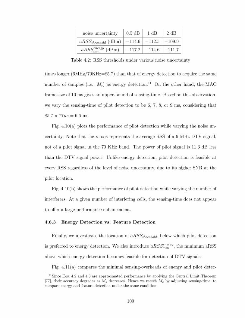
noise uncertainty 0.5 dB 1 dB 2 dB

aRSSthreshold (dBm) −114.6 −112.5 −109.9

aRSSenergymin (dBm) −117.2 −114.6 −111.7

Table 4.2: RSS thresholds under various noise uncertainty

times longer (6MHz/70KHz=85.7) than that of energy detection to acquire the same

number of samples (i.e., Ms) as energy detection.11 On the other hand, the MAC

frame size of 10 ms gives an upper-bound of sensing-time. Based on this observation,

we vary the sensing-time of pilot detection to be 6, 7, 8, or 9 ms, considering that

85.7× 77µs = 6.6 ms.

Fig. 4.10(a) plots the performance of pilot detection while varying the noise un-

certainty. Note that the x-axis represents the average RSS of a 6 MHz DTV signal,

not of a pilot signal in the 70 KHz band. The power of pilot signal is 11.3 dB less

than the DTV signal power. Unlike energy detection, pilot detection is feasible at

every RSS regardless of the level of noise uncertainty, due to its higher SNR at the

pilot location.

Fig. 4.10(b) shows the performance of pilot detection while varying the number of

interferers. At a given number of interfering cells, the sensing-time does not appear

to offer a large performance enhancement.

4.6.3 Energy Detection vs. Feature Detection

Finally, we investigate the location of aRSSthreshold, below which pilot detection

is preferred to energy detection. We also introduce aRSSenergymin , the minimum aRSS

above which energy detection becomes feasible for detection of DTV signals.

Fig. 4.11(a) compares the minimal sensing-overheads of energy and pilot detec-

11Since Eqs. 4.2 and 4.3 are approximated performance by applying the Central Limit Theorem[77], their accuracy degrades as Ms decreases. Hence we match Ms by adjusting sensing-time, tocompare energy and feature detection under the same condition.

109

# of interferers 1 2 4 6

aRSSthreshold (dBm) −112.9 −112.3 −111.3 −110.5

aRSSenergymin (dBm) −115.4 −115.1 −114.5 −114

Table 4.3: RSS thresholds under various inter-CRN interference

tion under various noise uncertainty conditions. With no noise uncertainty, energy

detection is the best to use. As the noise uncertainty grows, however, pilot detec-

tion becomes preferable at a low aRSS and aRSSthreshold increases accordingly. The

position of aRSSthreshold is shown in Table 4.2 along with aRSSenergymin . With 1 or 2

dB noise uncertainty, pilot detection becomes feasible and preferable even at −120

dBm, but it incurs more than 10% of sensing overhead.

aRSSthreshold and aRSSenergymin of various inter-CRN interference are also presented

in Fig. 4.11(b) and Table 4.3. With 1 or 2 dB noise uncertainty, pilot detection incurs

more than 15% of sensing overhead at −120 dBm.

From Tables 4.2 and 4.3, one can see that the feasibility region of energy detection

is reduced just by 1.4 dB between 1 cell and 6 cells, whereas the gap is 5.5 dB between

noise uncertainty of 0.5 dB and 2 dB. As a result, noise uncertainty seems to have a

more significant influence on energy-detection’s performance.

Other Feature Detectors

From Figs. 4.11(a) and 4.11(b), one can observe that energy detection, above

aRSSthreshold, incurs at most 0.385% of sensing overhead. Here, we compare this

overhead with three other types of feature detectors than pilot-energy detection: the

pilot-location detection in [19], the PN511 detection in [18], and the cyclostationary

detection in [11]. Since sensing-times for such feature detectors are 30 ms, 24.1 ms,

and 19.03 ms, respectively, their sensing overheads are given as at least 1.5, 1.2, and

0.95 % even when sensing is scheduled only once every CDT seconds. Therefore, en-

110

noise uncertainty 0 0.5 1 2 # of interferers 1 2 4 6

Nmin 1 5 24 221 Nmin 30 38 58 86

Table 4.4: The minimum number of sensor (Nmin) necessary for energy detection tobecome feasible at aRSS = IDT

ergy detection performs better in its preferred region (i.e., above aRSSthreshold) than

the pilot-energy as well as other three types of feature detectors under consideration.

4.6.4 Minimum Number of Sensors for Feasible Energy Detection ataRSS = IDT

As shown in Fig. 4.6(b), the performance of collaborative sensing improves as N

grows. Thus, as we increase N , aRSSenergymin also becomes smaller. This means that

we can find a minimum N , denoted by Nmin, with which energy detection can be

feasible even at aRSS = IDT . Here we investigate such Nmin and its relationship

with other optimization parameters, such as TI and TP .

Fig. 4.12 illustrates the tradeoff between sensing-overhead and Nmin. As we allow

higher sensing-overhead by introducing longer TI and smaller TP , we can achieve the

same target detection performance (i.e., PCDTMD = 0.1 and PCDT

FA = 0.1) with smaller

N , and vice versa. Therefore, to find Nmin, we allow maximum possible overhead,

TI = 770 µs and TP = 10 ms, in the scenario considered in Section 4.6.2. Then,

the corresponding Nmin becomes the lower bound of all possible N ’s below which no

energy detection becomes feasible at aRSS = IDT . Table 4.4 shows the Nmin for

various noise uncertainty and inter-CRN interference. In both cases, the maximum

Nmin (i.e., 221 and 86) does not exceed 331 sensors, which is the maximum number

of sensor in a cluster derived in Section 4.4.

111

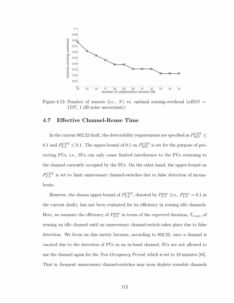
24 25 26 27 28 29 30 31 32 33 34 350

0.01

0.02

0.03

0.04

0.05

0.06

0.07

0.08

0.09

0.1

min

ima

l se

nsi

ng

-ove

rhe

ad

number of collaborative sensors (N)

Figure 4.12: Number of sensors (i.e., N) vs. optimal sensing-overhead (aRSS =IDT , 1 dB noise uncertainty)

4.7 Effective Channel-Reuse Time

In the current 802.22 draft, the detectability requirements are specified as PCDTMD ≤

0.1 and PCDTFA ≤ 0.1. The upper-bound of 0.1 on PCDT

MD is set for the purpose of pro-

tecting PUs, i.e., SUs can only cause limited interference to the PUs returning to

the channel currently occupied by the SUs. On the other hand, the upper-bound on

PCDTFA is set to limit unnecessary channel-switches due to false detection of incum-

bents.

However, the chosen upper-bound of PCDTFA , denoted by Pmax

FA (i.e., PmaxFA = 0.1 in

the current draft), has not been evaluated for its efficiency in reusing idle channels.

Here, we measure the efficiency of PmaxFA in terms of the expected duration, Treuse, of

reusing an idle channel until an unnecessary channel-switch takes place due to false

detection. We focus on this metric because, according to 802.22, once a channel is

vacated due to the detection of PUs in an in-band channel, SUs are not allowed to

use the channel again for the Non-Occupancy Period, which is set to 10 minutes [84].

That is, frequent unnecessary channel-switches may soon deplete reusable channels

112

even if there are many idle ones.

Thus, we would like to see if the requirement PmaxFA = 0.1 is strict enough by

analyzing Treuse for a given PmaxFA , and determine a proper Pmax

FA allowing practically

long enough reuse of idle channels. For this purpose, we consider periodic in-band

sensing, as in Fig. 4.4, on an idle channel during its long OFF period, where we

assume that each sensing operation is performed by N cooperating sensors with PFA

as the single-sensor’s false alarm probability.

First, we denote PFA(N) by PNFA for notational simplicity, and express Eq. (4.7) as

a function of PNFA, i.e., the false alarm probability of single-time cooperative sensing

as given in Eq. (4.1), as follows

PCDTFA (PN

FA) = 1−∑M

(1− PN

FA

)Mp(M). (4.8)

Then, it is trivial to show that Eq. (4.8) is a monotonic increasing function of PNFA.

Hence, having PCDTFA upper-bounded by Pmax

FA is the same as having PNFA upper-

bounded by PmaxFA , where PCDT

FA (PmaxFA ) = Pmax

FA .

Next, the expected channel-reuse duration, Treuse, is derived as

Treuse = TP · (1− PNFA)PN

FA + 2TP · (1− PNFA)2PN

FA + · · ·

=∞∑i=0

iTP · (1− PNFA)iPN

FA = TP

(1− PN

FA

PNFA

). (4.9)

Therefore, the smaller PNFA, the longer an idle channel can be reused without false

detection of PUs. This implies that we need to set PmaxFA small enough to make Treuse

reasonably large.

We now want to evaluate the efficiency of the current detectability requirement in

the 802.22 draft, i.e., PmaxFA = 0.1. While varying Pmax

FA from 0.001 to 0.1, we compute

Nmin for each PmaxFA value, where Nmin is defined the same as in Section 4.6.4. Then,

for each pair (PmaxFA , Nmin), our in-band sensing scheduling algorithm is applied to

113

determine the optimal sensing-period TP and sensing-time TI with minimal sensing

overhead. Finally, we calculated Treuse using the chosen PmaxFA , the derived TP , and

Eq.(4.9). The results are plotted in Fig. 4.13.

As shown in Fig. 4.13(a), Treuse at PmaxFA = 0.1 turns out to be just 20 seconds.

That is, with the currently-chosen upper-bound 0.1, a WRAN can reuse an idle

channel for an average of only 20 seconds before making an unnecessary channel-

switch. This implies that a WRAN may require at least 30 idle channels exclusively

assigned for its use to provide a seamless service to CPEs, considering the Non-

Occupancy Period of 10 minutes. However, there are only 68 channels in TV bands,

and thus, it is unlikely to have 30 concurrently idle channels while there are many

active TV stations. In addition, self co-existence between neighboring WRANs will

make it harder to find an enough number of idle channels reserved for a certain

WRAN.

To resolve this issue, we can impose a much more strict upper-bound on the

false alarm probability by reducing PmaxFA significantly. Fig. 4.13(a) indicates that

by using PmaxFA = 0.001, the expected channel-reuse time is enhanced by two orders-

of-magnitude (i.e., E[Treuse] = 2, 000 seconds) which is reasonably long for SUs to

operate on an idle channel. Although one may wonder if the new constraint on

PmaxFA might increase Nmin and the sensing overhead significantly, Figs. 4.13(b) and

4.13(c) show a minimal increase in Nmin (just 3 more sensors) and a bounded sensing

overhead between 0.069 and 0.077 when PmaxFA varies.

As a result, we recommend PmaxFA = 0.001 as a new requirement on the false-alarm

probability. Using this new value of PmaxFA , combined with the proposed in-band

sensing scheduling, we can still meet the detectability requirements with a slight

increase in the number of collaborative sensors while enhancing the channel-reuse

114

time significantly.

4.8 Conclusion

In this chapter, we discussed three important aspects of in-band spectrum sensing

in the IEEE 802.22: sensor clustering, sensing scheduling, and detectability require-

ments. First, we showed the necessity of sensor clustering and derived the maxi-

mum sensor cluster size and sensor density. Next, we proposed an in-band sensing

scheduling algorithm that minimizes sensing-overhead while meeting the detectabil-

ity requirements, and evaluated its performance with respect to noise uncertainty

and inter-CRN interference. We also derived the SNR threshold above which energy

detection is preferred to feature detection and the minimum number of collabora-

tive sensors for feasible energy detection at a given SNR. Finally, we investigated

how strict the detectability requirement must be to guarantee efficient channel reuse

without incurring unnecessarily often channel-switches.

115

10-3

10 -2

10 -1

101

102

103

104

upper bound of PFACDT

T

reu

se (in s

eco

nds)

(a) Expected Treuse

10-3

10 -2

10 -1

24

25

26

27

upper bound of PFA

CDT

Nm

in

(b) Nmin

10-3

10 -2

10 -1

0.068

0.07

0.072

0.074

0.076

0.078

upper bound of PFA

CDT

optim

al sensin

g o

verh

ead

(c) Sensing overhead TI/TP

Figure 4.13: Treuse, Nmin, and sensing overhead TI/TP with varying PmaxFA

116

CHAPTER V

WHITESPACE UTILIZATION PART I:

OPTIMAL CONTROL OF SECONDARY

USERS FOR PROFIT MAXIMIZATION AT CR

SERVICE PROVIDERS

5.1 Introduction

The application of dynamic spectrum access (DSA) ranges from public to com-

mercial and military networks. In this chapter, we focus on a commercial DSA

application, cognitive radio (CR) Wi-Fi hotspots, which is an attractive and promis-

ing example of DSA. A CR Wi-Fi hotspot (henceforth simply referred to as CR

hotspot) consists of a CR access point and CR-enabled customer terminals where a

CR wireless service provider (WSP) opportunistically utilizes the licensed spectrum

to provide Internet access to the CR customers. The use of spectrum whitespaces

for this Wi-Fi-like service has been identified as an important step in DSA de-

velopment, due to its similarity to today’s Wi-Fi and more favorable propagation

characteristics of the licensed spectrum (e.g., TV bands) than the ISM bands like

larger coverage and the wall-penetrating ability [10]. Although the Wi-Fi-like service

over whitespaces has been given different names such as Wi-Fi 2.0 [22], WhiteFi [3],

and 802.11af [48], this chapter focuses on its general aspects of customer flow control

117

A Pool of Licensed spectrum

Spectrum Lease

• Temporal usage right transfer

(e.g., periodic spectrum auction)

End-Customers

(CR devices)

Wireless Service Providers(CR Hotspots)

Service Provisioning

Spectrum plane Service plane

Spectrum

Broker

User plane

• Short-term contract

(e.g., by sessions)

Figure 5.1: Inter-plane interactions in the dynamic spectrum market

under the time-varying spectrum availability.1

The concept of CR hotspots can be better understood in the framework of dy-

namic spectrum market (DSM) [44] (also called secondary market) in which the

primary license holders can temporarily transfer their spectrum usage rights to CR

users. The DSM consists of three interacting layers/planes—spectrum, service, and

user planes—as shown in Fig. 5.1. In the spectrum plane, a spectrum broker (SB)

leases licensed spectrum to the (CR) WSPs at the service plane, where the SB is

either the regulatory authorities (e.g., FCC in USA and Ofcom in UK) or an autho-

rized third-party. The WSPs compete with each other to lease as many spectrum

bands as necessary which will be opportunistically utilized to provide the CR hotspot

service to the CR users at the user plane.

The dynamic spectrum lease can be described by one of the three prevailing mod-

els in the CR literature: dynamic exclusive-use, shared-use, and private commons [5].

In the dynamic exclusive-use model, licensees can dynamically lease their spectrum

to the lessees (i.e., secondary users (SUs)) who temporarily own an exclusive right

to access the spectrum, but the spectrum leasing is not performed in real-time and

the SUs’ service should be the same type as the licensees. In the shared-use model,

1Note that Wi-Fi over whitespaces is not necessarily based on the same type of protocol as IEEE802.11, as pointed out in [48].

118

SUs are allowed to freely access licensed bands opportunistically in the absence of

primary users (PUs), without paying any leasing fees. Lastly, the private commons

model enables more flexible integration of DSA in the licensed spectrum via real-time

spectrum leasing by the dynamic spectrum auction where the licensees can also set

their own rules on how their spectrum is used by the SUs. Among the three models,

the private commons model is believed to be a viable market option that benefits

both licensees and CR users [5] since the licensees can make extra profit via spectrum

leasing (unlike shared-use) and the CR users are given full flexibility in utilizing the

whitespaces (unlike dynamic exclusive-use).

5.1.1 Contributions

Our contribution in this chapter is two-fold. First, we propose a new spectrum

reuse model called preemptive spectrum lease which is a realization of the private

commons, as illustrated in Fig. 5.2. In our model, the license holders temporarily

lease their channels to CR WSPs via periodic dynamic spectrum auction (e.g., hourly)

and charge them for their opportunistic use of paid-but-idle channels. The WSPs

are allowed to use the leased channels only when they are temporarily unoccupied by

the PUs because the licensed users are given priority over the unlicensed CR users.

Therefore, the CR users must vacate a channel to which PUs return (called channel

vacation) where the channel state changes from ‘available to SUs’ to ‘occupied by

PUs’, and should utilize the remaining idle channels afterwards. When PUs no longer

transmit on the vacated channel, it can be used again by the SUs. Once a leasing

term ends, the leased channels are all returned to the licensees and the WSPs must

re-participate in the auction to lease new channels.

Next, we solve the profit maximization problem of a WSP by optimizing two types

119

ON

OFF

ON

OFF

ON

OFF

3 leased channels 4 leased channels 2 leased channels

…

Leasing period (utilizes only OFF periods)

Return leased channels è Re-participate the auction

Figure 5.2: The preemptive spectrum lease model

of user control: admission and eviction. Admission control determines if a newly-

arriving customer should be admitted to or rejected from the service, to achieve better

profit. Although optimal user admission control in isolation was studied in [66] for

the case of static spectrum availability, CR networks face a unique challenge—time-

varying spectrum availability due to PUs’ activities—that necessitates joint control of

user admission and eviction. At channel vacation, the customers previously assigned

to the channel (called in-service users) have to be relocated by the WSP to the

other remaining idle channels. However, in case the remaining idle channels cannot

fully support spectrum demands of all in-service users,2 the WSP should determine

which users to be evicted from its network. The evicted users will be compensated

with some form of reimbursement, which may differ by the user-specific spectrum

demands and thus affect the WSP’s profit.

To derive the optimal user admission and eviction controls, we first model it as a

semi-Markov decision process (SMDP) and a linear programming (LP) algorithm is

2QoS degradation (i.e., assigning less bandwidth than a user requested) is not considered in thischapter, which is our future work.

120

proposed to derive the solution. QoS provisioning for CR end-users is also considered

by adding two constraints to the LP algorithm: the probability of blocking newly-

arriving users and the probability of evicting/dropping in-service users, so that the

WSP can strike a balance between profit maximization and customer satisfaction.

5.1.2 Organization

The rest of the chapter is organized as follows. Section 5.2 overviews related work,

and then Section 5.3 introduces the system model and the basic assumptions used

throughout this chapter. In Section 5.4, the problem of maximizing a WSP’s profit is

modeled as an SMDP and its relevant components are derived. Section 5.5 presents

an LP-based SMDP algorithm to determine the optimal user admission and eviction

policies with constraints on the blocking and dropping probabilities. Section 5.6

introduces a prioritized multi-class service at CR hotspots and derives its optimal

user controls. The proposed scheme is evaluated in Section 5.7 via numerical analysis

and in-depth simulation, and the chapter concludes with Section 5.8.

5.2 Related Work

Mutlu et al. [58] studied how to maximize a WSP’s average profit, focusing on

an optimal pricing policy without considering user admission control which could

increase the WSP’s profit further. Moreover, they assumed that PUs and SUs can

simultaneously access the same channel, thus unneeding user eviction control, which

is not possible if PUs are given priority over SUs. Ishibashi et al. [43] considered

multi-homed PUs, where each PU is either conventional or CR-enabled. They inves-

tigated enhancement of resource utilization with cognitive PUs switching between

channels, and derived the blocking and dropping probabilities in such a scenario.

However, no priority in channel access is given to the conventional PUs, thus unac-

121

counting for user eviction. Wang et al. [95] proposed a primary-prioritized Markov

approach where PUs have exclusive rights to access their own channels. Although

they considered giving priority to PUs, user admission control was ignored and only

one channel and two SUs were considered, thus limiting its applicability. Ross and

Tsang [66] investigated the problem of optimal admission control on the users with

different spectrum demands. However, their problem was limited to the case when

channels are always available, thus unneeding user eviction control.

5.3 System Model

In this section, we introduce the system model and assumptions to be used

throughout this chapter.

5.3.1 Channel Model

A channel is modeled as an ON/OFF alternating renewal process, as introduced

in Chapter I. It is assumed that the transitions between ON and OFF states can be

detected by either spectrum sensing or a PU signalling mechanism. First, spectrum

sensing, as described in Chapter I, is a process of sampling the channel state (i.e., ON

or OFF) to identify spectrum whitespaces, which has been discussed in Chapters II,

III, and IV. Second, the PU signalling mechanism is a method with which the

licensee indicates the presence/absence of the PUs in its channels so that the lessee

can notice the status of the leased channels. Since the licensee can achieve extra profit

via spectrum leasing, it is reasonable to assume that the licensee may be willing to

build such an auxiliary mechanism to entice more CR WSPs to the secondary market

and to protect its PUs more effectively.

Let Ci denote the capacity (or bandwidth) of channel i. In this chapter, we

assume channel capacities are homogeneous, i.e., Ci = C, ∀i, for ease of presentation.

122

ON

OFF

ON

OFF

ON

OFF

3

2

1

0

Number of idle

channels m:

Figure 5.3: Time-varying channel capacity

However, our SMDP model can be easily extended to the case of heterogeneous

channel capacities at the expense of increased state/action spaces. With M (possibly

non-contiguous) leased channels, a WSP’s instantaneous capacity is given as m · C,

0 ≤ m ≤ M , according to the ON/OFF channel-usage patterns, where m is the

number of idle channels (i.e., channels in their OFF states) at that instant as shown

in Fig. 5.3. We assume that the pool of idle channels is treated as one logical channel,

whose capacity is equal to m · C bandwidth-units. This can be realized by the

Orthogonal Frequency Division Multiplexing (OFDM) techniques with adaptive and

selective allocation of OFDM sub-carriers, like NC-OFDM (Non-Contiguous OFDM)

proposed in [64].

5.3.2 Spectrum Auction Model

We consider a multi-winner periodic spectrum auction [30,97] where an SB (auc-

tioneer) auctions off the licensed channels periodically (e.g., hourly, daily, or even

weekly) every Tauction, and multiple WSPs bid for the number of channels they want

to lease. Once a WSP wins M channels, it pays the (leasing) price of pbid(M) per

unit-time to obtain temporary rights to reuse the channels for the period of Tauction.

123

After Tauction, the leased channels are returned to the licensees.

We make the following assumption on the bidding cost function pbid(M), pbid(0) =

0, which is commonly accepted in the the CR auction market literature [44,61].

Assumption 1. pbid(M) is a positive, non-decreasing and convex function of M .

This assumption is reasonable because the winning bid is likely to increase faster

than proportionally to M due to the competition between WSPs contending for the

limited amount of spectrum resources auctioned off in the market. The actual form

of pbid(M) should depend on the auction market, and hence, we assume pbid(M) is

given a priori in order to focus on user-control issues. For an illustrative purpose,

our simulation in Section 5.7 will use pbid(M) = D1 · MD2 , D2 ≥ 1, which was

introduced in [44,61] and satisfies Assumption 1. Note that D2 represents the degree

of competition in the auction.

5.3.3 Multi-class User QoS Model

A customer at a CR hotspot is a CR-capable device that is assumed to have a

spectrum demand in one of the following K QoS-classes:

B = (B1, B2, . . . , BK)T,

where Bk is the bandwidth requirement of class-k customers and T represents ‘trans-

pose’. Without loss of generality, we can assume Bmin = B1 < B2 < . . . < BK =

Bmax. Note that we reserve k as the index of user class.

Based on selective OFDM sub-carrier allocation, each CR user is assumed to be

capable of tuning its antenna to any portion of the logical channel for its bandwidth

assignment of Bk, as illustrated in Fig. 5.4. In this way, at a channel’s OFF→ON

transition, the users on the channel can be redistributed to other idle channels, by

124

CH 1

CH 2

User 2 (B3=3)User 1 (B2=2)

User 3 (B1=1)

User 4 (B1=1)

User 5 (B1=1)

User 6 (B1=1)

User 7 (B1=1)

Figure 5.4: An example of channel allocation with M = 2, K = 3, and C = 5.

updating the mapping of OFDM subcarriers to the users. MAC-layer beaconing

might be used to perform this re-mapping in real time.

We assume the arrival of class-k customers follows the Poisson distribution with

rate λk, since the service requests from the CR users are made at the connection level

and user-oriented connection requests are modeled well as a Poisson process [63].

For mathematical tractability, the service time of an in-service class-k customer is

assumed exponentially distributed with mean 1/µk, capturing the reality of some

applications such as phone-call traffic with exponentially-distributed talk spurt [87].

5.3.4 End-User Pricing Model

The revenue of a WSP is generated by the CR end-users who pay fees for their

opportunistic spectrum usage. The vector of the usage fees for K QoS-classes, in

terms of price per unit-time per unit-bandwidth, is denoted by

p = (p1, p2, . . . , pK)T.

The arrival rate is price-dependent, and therefore, it is represented by λk(pk).

λk(pk) is a non-increasing function of pk, since a WSP advertising higher prices

should expect less customer arrivals than the others offering lower prices. The actual

125

price-arrival relationship depends strongly on the WSP’s tariff and the degree of

competition, which must be treated as a separate marketing problem. Here we

assume λk(pk) is given a priori and confine our discussion to the optimal user control.

We leave λk(pk) as a general parameter in the analysis, and in Section 5.7 we will

use an example of λk(pk) = λmaxk e−δkpk as introduced in [29], for an illustrative

purpose. Here, λmaxk indicates that the maximum user population at a CR hotspot

is bounded, and δk represents the rate of decrease of the arrival rate as pk increases,

which is related to the degree of competition between WSPs.

5.4 SMDP Formulation

The profit maximization at a CR hotspot poses a unique challenge due to time-

varying channel availability that necessitates joint user admission and eviction control

by the CR WSP. In such a case, SMDP is a useful tool to determine the optimal

actions achieving maximal profit, and thus in this section we formulate the system

as an SMDP. We first show the validity of SMDP formulation for the problem con-

sidered, and then we derive the basic and essential components of the SMDP by

accounting for time-varying channel availability and possible actions to be taken for

user admission and eviction. In Section 5.5, we will use the derived components

to construct our proposed LP algorithm that determines the optimal actions and

achieves the maximal profit.

5.4.1 System State and State Space

We start with the definition of system state as

s = (n,w), and

n = (n1, n2, . . . , nK)T,

w = (w1, w2, . . . , wM)T,

(5.1)

126

where nk is the number of class-k customers in service, and wi is the channel state

defined as

wi =

1, channel i is occupied by PUs (i.e., ON),

0, channel i is not occupied by PUs (i.e., OFF).

Then, the sub-state-space of w, denoted by Λw, and the sub-state-space of n given

w, denoted by Λn|w, are defined as

Λw = {w : wi ∈ {0, 1}},

Λn|w = {n : nk ≥ 0, nTB ≤ mC, m = (1−w)T1},

where m is the number of idle channels and 1 is a vector of 1’s. Therefore, the state

space Λ is given as

Λ = {s : w ∈ Λw,n ∈ Λn|w}.

5.4.2 Possible Actions and Action Space

In our SMDP formulation, an action is taken and updated at each decision epoch

under the chosen policy, where a natural choice of the decision epoch is the instant

when a channel’s state changes, i.e., (1) at a class-k customer’s arrival/departure

and (2) at channel i’s state-transition (ON→OFF or OFF→ON).

We define the action at a certain decision epoch as

α = (a,b), and

a = (a1, a2, . . . , aK)T,

b = (b1, b2, . . . , bK)T,

where a is the admission policy for future customer arrivals such that

ak =

0, reject all future class-k arrivals,

1, admit all future class-k arrivals,

127

and b is the eviction policy for in-service customers where bk indicates the number

of class-k customers to be evicted at the time of channel vacation, i.e., at state-

transition OFF→ON on a certain channel. That is, even if b 6= 0, we do not evict

any customer if the next event is an arrival, departure, or state-transition ON→OFF.

Then, for a given state s, the action space A is defined as

A(s) =

{α : a = 0, b = 0} , if m = 0,

{α : a ∈ A1(s), b ∈ A2(s)} , otherwise,

(5.2)

with A1(s) and A2(s) being defined as

A1(s) = { a : ak ∈ {0, 1}; ak = 0 if (n + uk)TB > mC } , (5.3)

A2(s) = { b : 0 ≤ bk ≤ nk; b = 0 if nTB ≤ (m− 1)C;

(n− b + uk)TB > (m− 1)C, for ∀k s.t.

bk 6= 0, and (n− b)TB ≤ (m− 1)C } , (5.4)

where uj is a unit vector with a single 1 at the j-th position and 0’s elsewhere. In

the definition of A2(s), the constraint

(n− b + uk)TB > (m− 1)C for ∀k s.t. bk 6= 0

implies that b should be minimal so as not to evict more in-service customers than

necessary. That is, b is not minimal if there exists k such that b′ = b − uk and

(n − b′)TB ≤ (m − 1)C, i.e., evicting one less customer than b still fits in (m − 1)

channels. Obviously, the choice of minimal b for given s is not unique. For example,

in case m = 2, C = 5 and B = (1, 2), there are three possible minimal b’s for

n = (5, 2): b = (4, 0), b = (2, 1) and b = (0, 2).

128

5.4.3 Validity of SMDP Formulation

Before deriving the other essential components of the SMDP, we need to check if

the system under consideration can be modeled as an SMDP. In [93], an SMDP is

defined as follows.

Definition 1. A dynamic system is said to be a semi-Markov decision process if the

following property is satisfied: if at a decision epoch the action α is chosen in state

s, then the time until the state at, and revenue/cost incurred until, the next decision

epoch depend only on s and α.

To check if a system under consideration satisfies Definition 1, we first consider

(1) a combined process of K-class user arrivals and departures, (2) M independent

processes of channel-state transitions, and (3) a combined process of (1) and (2).

A combined process of user arrivals and departures

Inter-arrival and inter-departure times of class-k customers are all assumed to

be exponentially distributed. Since the arrival and departure processes are indepen-

dent of each other, the inter-event time, denoted by T0, of the combined random

process is also exponentially distributed with mean 1/ρ, where ρ := nTµ + aTλ,

λ = (λ1, λ2, . . . , λK)T, and µ = (µ1, µ2, . . . , µK)T.

M independent processes of channel-state transitions

For generally-distributed ON/OFF periods, the time until the next state-transition

on channel i depends not only on wi but also on the elapsed time since the last state-

transition, denoted by ei. To satisfy the conditions in Definition 1, the previous

definition of state s can be extended as

s = (n,w, e), e = (e1, e2, . . . , eM)T.

129

This approach, however, is impractical since ei is continuous, introducing infinitely

many possible states.

To derive a mathematically tractable but reasonably accurate model, we take an

approximation-based approach using renewal theory [20] as follows.

Proposition 1 (Cox [20]). Given that a renewal process of channel i has started

a long time ago, the residual time in the current state, regardless of how much time

has elapsed since the last state-transition, has the pdf of

(1− FT iOFF

(t))/E[T iOFF ], t > 0, if wi = 0,

(1− FT iON

(t))/E[T iON ], t > 0, if wi = 1,

(5.5)

where FT iOFF

(t) and FT iON

(t) are the cumulative distribution functions (cdfs) of T iOFF

and T iON .

Proposition 1 indicates that as the current time progresses farther away from the

time origin of a renewal channel, the pdf of the remaining time until the next state-

transition will converge to Eq. (5.5). Note that exponential distribution is the only

instance with which Eq. (5.5) coincides with fT iOFF

(t) and fT iON

(t).

Using this property, we can keep the definition of s same as Eq. (5.1) while

approximating the system as an SMDP because the pdfs in Eq. (5.5) do not depend

on ei’s and are thus memoryless. In Section 5.7, we will show that this approximation,

in fact, produces reasonably accurate results.

The overall combined process

Using the fact that the combined arrival/departure process and renewal processes

of M channels are independent of each other, the cdf of the remaining time T until

130

the next decision epoch is given as

P (T ≤ t) = 1− P (T = min(T0, T1, . . . , TM) > t)

= 1− P (T0 > t, T1 > t, . . . , TM > t)

= 1−M∏

l=0

P (Tl > t) = 1−M∏

l=0

(1− P (Tl ≤ t)),

(5.6)

where Tl (1 ≤ l ≤ M) is a random variable representing the residual time until the

next state-transition on channel l whose pdf is given as Eq. (5.5).

As a result, the system model considered in this chapter becomes an SMDP since

it possesses the properties in Definition 1:

• The time until the next decision epoch depends only on (s, α) since Eq. (5.6)

is a function of n, a, w.

• The state s′ = (n′,w′) at the next decision epoch depends only on s and α

such that (1) n′ = n + uk, w′ = w, at a class-k user’s arrival, (2) n′ = n− uk,

w′ = w, at a class-k user’s departure, (3) n′ = n− b, w′ = w + ui, at channel

i’s OFF→ON transition, and (4) n′ = n, w′ = w−ui, at channel i’s ON→OFF

transition.

• The revenue and cost accrued until the next decision epoch depend only on s

and α since they are a function of n, b, and the time until the next decision

epoch. The definition of revenue and cost will be detailed in Section 5.4.6.

5.4.4 Decision Epochs

The expected time between two decision epochs, denoted by τs(α), is determined

as

τs(α) =

∫ ∞

0

tfT (t)dt, fT (t) =dP (T ≤ t)

dt,

131

where P (T ≤ t) is from Eq. (5.6).

For example, with exponentially-distributed ON and OFF durations with mean

1/µiON and 1/µi

OFF , the expected time between two decision epochs is determined

as

τs(α) =[nTµ + aTλ + (1−w)TµOF F + wTµON

]−1,

where µOF F = (µ1OFF , µ2

OFF , . . . , µMOFF )T and µON = (µ1

ON , µ2ON , . . . , µM

ON)T. This

result can be understood intuitively as follows. Since channel i’s residual time in

ON (or OFF) state is exponentially distributed with mean 1/µiON (or 1/µi

OFF ), the

time between state-transitions becomes exponentially distributed with mean 1/((1−

wi)µiOFF +wiµ

iON). Therefore, with M independent channels, the combined random

process is also exponentially distributed with mean[(1−w)TµOF F + wTµON

]−1.

As a result, the combined process of user arrivals/departures with M channel state-

transitions becomes exponentially distributed with mean[nTµ + aTλ + (1−w)TµOF F

+wTµON

]−1.

5.4.5 State-Transition Probability

The probability that the state of the SMDP switches from s = (n,w) to s′ =

(n′,w′) at the next decision epoch is given as in Eq.(5.7), where Ta, T−a, Td, and

T−d are exponentially-distributed random variables with mean 1/akλk, 1/(ρ− akλk),

1/nkµk, and 1/(ρ− nkµk).

132

ps,s′(α) =

P (Ta ≤ T−a, Ta ≤ T1, . . . , Ta ≤ TM), at a class-k user’s arrival,

P (Td ≤ T−d, Td ≤ T1, . . . , Td ≤ TM), at a class-k user’s departure,

P (Ti ≤ T0, Ti ≤ T1, . . . , Ti ≤ TM), at channel i’s OFF↔ON,

=

∫∞0

∫∞ta· · · ∫∞

ta

{fTa(ta)fT−a(t−a)fT1(t1) · · · fTM

(tM)}dt−adt1 · · · dtMdta,∫∞

0

∫∞td· · · ∫∞

td

{fTd

(td)fT−d(t−d)fT1(t1) · · · fTM

(tM)}dt−ddt1 · · · dtMdtd,∫∞

0

∫∞ti· · · ∫∞

ti{fT0(t0)fT1(t1) · · · fTM

(tM)}dt0 dt1 · · · dtM︸ ︷︷ ︸except ti

dti.

(5.7)

For example, for exponentially-distributed ON/OFF periods, we have

ps,s′(α) =

akλkτs(α), n′ = n + uk, w′ = w, class-k arrival,

nkµkτs(α), n′ = n− uk, w′ = w, class-k departure,

µiOFF τs(α), n′ = n− b, w′ = w + ui, channel i: OFF→ON,

µiONτs(α), n′ = n, w′ = w − ui, channel i: ON→OFF.

5.4.6 Revenue and Reimbursement Cost

Let rs(α) and cs(α) denote the expected revenue and the cost incurred by cus-

tomers until the next decision epoch if action α is chosen at state s, respectively.

Since the revenue comes from the usage fee paid by the admitted customers, rs(α)

is given as

rs(α) =∑

k

pkBknkτs(α).

Assuming a fixed amount of reimbursement Ik for an evicted class-k customer, cs(α)

is

cs(α) =∑

k

Ikbk · qVs (α),

133

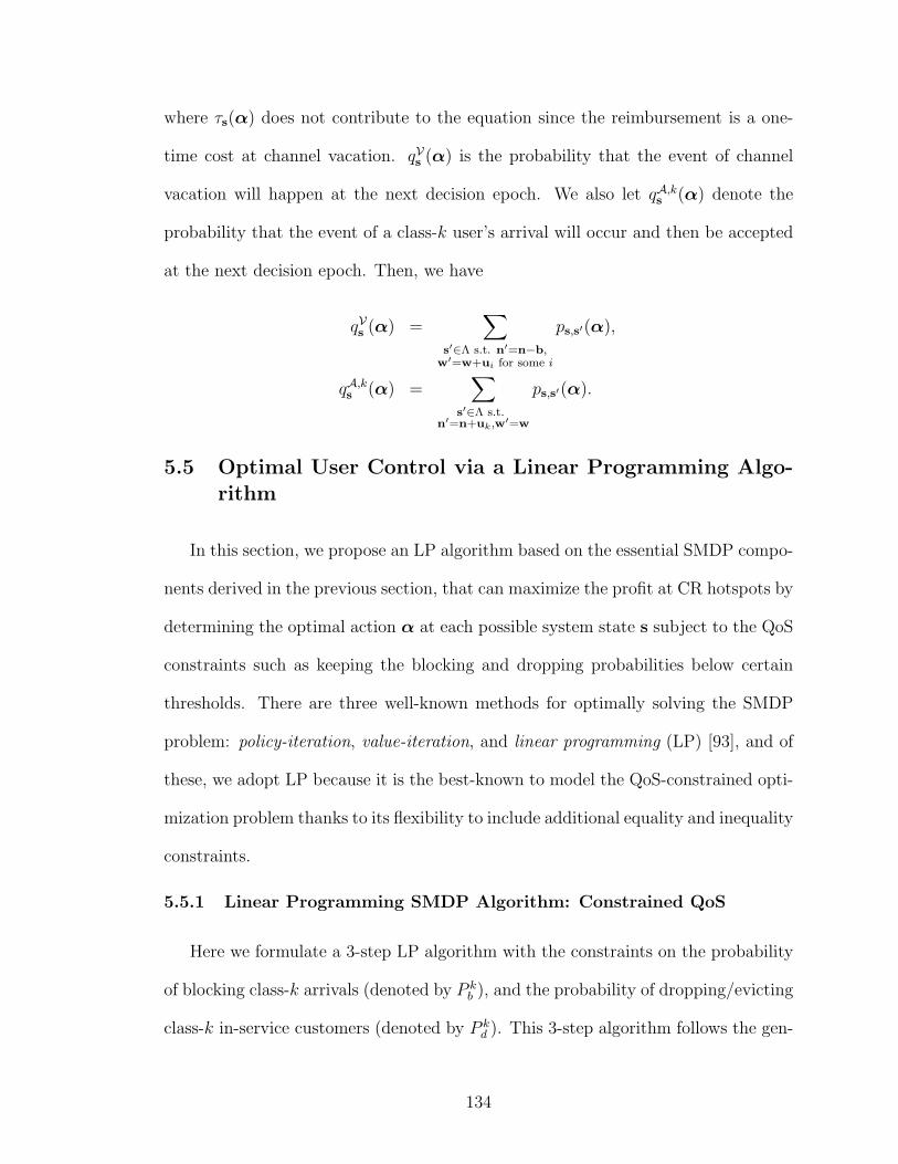
where τs(α) does not contribute to the equation since the reimbursement is a one-

time cost at channel vacation. qVs (α) is the probability that the event of channel

vacation will happen at the next decision epoch. We also let qA,ks (α) denote the

probability that the event of a class-k user’s arrival will occur and then be accepted

at the next decision epoch. Then, we have

qVs (α) =∑

s′∈Λ s.t. n′=n−b,w′=w+ui for some i

ps,s′(α),

qA,ks (α) =

∑

s′∈Λ s.t.n′=n+uk,w′=w

ps,s′(α).

5.5 Optimal User Control via a Linear Programming Algo-rithm

In this section, we propose an LP algorithm based on the essential SMDP compo-

nents derived in the previous section, that can maximize the profit at CR hotspots by

determining the optimal action α at each possible system state s subject to the QoS

constraints such as keeping the blocking and dropping probabilities below certain

thresholds. There are three well-known methods for optimally solving the SMDP

problem: policy-iteration, value-iteration, and linear programming (LP) [93], and of

these, we adopt LP because it is the best-known to model the QoS-constrained opti-

mization problem thanks to its flexibility to include additional equality and inequality

constraints.

5.5.1 Linear Programming SMDP Algorithm: Constrained QoS

Here we formulate a 3-step LP algorithm with the constraints on the probability

of blocking class-k arrivals (denoted by P kb ), and the probability of dropping/evicting

class-k in-service customers (denoted by P kd ). This 3-step algorithm follows the gen-

134

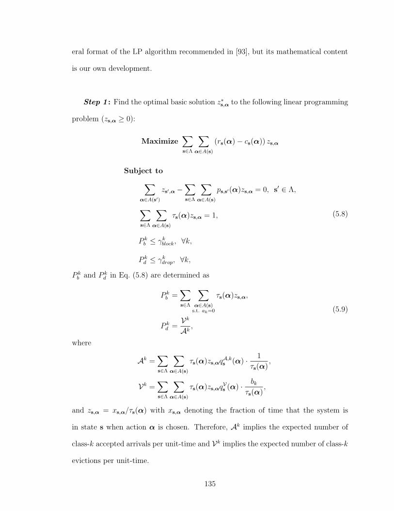
eral format of the LP algorithm recommended in [93], but its mathematical content

is our own development.

Step 1 : Find the optimal basic solution z∗s,α to the following linear programming

problem (zs,α ≥ 0):

Maximize∑s∈Λ

∑

α∈A(s)

(rs(α)− cs(α)) zs,α

Subject to

∑

α∈A(s′)

zs′,α −∑s∈Λ

∑

α∈A(s)

ps,s′(α)zs,α = 0, s′ ∈ Λ,

∑s∈Λ

∑

α∈A(s)

τs(α)zs,α = 1,

P kb ≤ γk

block, ∀k,

P kd ≤ γk

drop, ∀k,

(5.8)

P kb and P k

d in Eq. (5.8) are determined as

P kb =

∑s∈Λ

∑

α∈A(s)s.t. ak=0

τs(α)zs,α,

P kd =

Vk

Ak,

(5.9)

where

Ak =∑s∈Λ

∑

α∈A(s)

τs(α)zs,αqA,ks (α) · 1

τs(α),

Vk =∑s∈Λ

∑

α∈A(s)

τs(α)zs,αqVs (α) · bk

τs(α),

and zs,α = xs,α/τs(α) with xs,α denoting the fraction of time that the system is

in state s when action α is chosen. Therefore, Ak implies the expected number of

class-k accepted arrivals per unit-time and Vk implies the expected number of class-k

evictions per unit-time.

135

The form of P kd makes this a nonlinear programming (NLP) problem. Fortunately,

however, by properly manipulating the constraint P kd ≤ γk

drop, it can be converted to

a linear programming (LP) problem as follows:

Vk

Ak≤ γk

drop ⇒ Vk − γkdropAk ≤ 0

⇒∑s∈Λ

∑

α∈A(s)

(qVs (α) · bk − γk

dropqA,ks (α) · 1)zs,α ≤ 0,

which is a linear constraint on zs,α’s.

Step 2 : Start with a non-empty set

S :=

s|

∑

α∈A(s)

z∗s,α > 0

,

and for any state s ∈ S, set the decision as

R∗(s) := α for some α such that z∗s,α > 0.

Step 3 : If S = Λ, then the algorithm terminates with the optimal policy R∗.

Otherwise, determine some state s /∈ S and action α ∈ A(s) such that ps,s′(α) > 0

for some s′ ∈ S. For the chosen s, set R∗(s) := α and update S := S ∪{s}, and then

repeat Step 3.

By repeatedly performing Step 3, the algorithm runs until S becomes Λ. The

computational complexity of executing this final step is trivial since ps,s′(α) > 0

has already been computed in Step 1 for all possible combinations of (s, s′,α). In

addition, the optimality of the derived policy is guaranteed in [93], although the

algorithm may not produce a unique solution due to the conditions ‘some α’ and

‘some s′’ in Steps 2 and 3.

136

Then, the optimal profit g∗ per unit-time is determined as

g∗ =∑s∈Λ

α=R∗(s)

(rs(α)− cs(α))zs,α − pbid(M). (5.10)

5.5.2 Complexity of SMDP Algorithm

The complexity of the proposed algorithm is measured by the size of the search

space Λ×A(s). In Fig. 5.5, one can see that |Λ×A(s)| increases almost exponentially

as M or K increases, because |Λw| = 2M and |A1(s)| = 2K in the worst case.

However, the complexity issue can be managed properly in the real scenarios due to

the following two reasons.

First, in commercial applications, a reasonable range of (M, K) could be 1 ≤

K, M ≤ 3 in which case we have a moderate and reasonable level of complexity

since |Λ × A(s)| ≤ 2, 167 in Fig. 5.5. For example, K = 3 for a service with Gold,

Silver, and Bronze classes, and K = 2 for a service with Premium and Basic classes.

In fact, the premium/basic classification is commonly found in today’s commercial

Wi-Fi hotspot services. In addition, if we compare the effective capacity of our Wi-

Fi-like service over whitespaces with that of the traditional Wi-Fi, a CR hotspot

utilizing M ON/OFF channels has M · (1−u)C provided the channels have a similar

utilization factor of u such that

u = E[T iON ]/{E[T i

ON ] + E[T iOFF ]},

while the traditional Wi-Fi utilizing a single and always-idle channel has C. In prac-

tice, licensed bands with lower utilization (e.g., u < 0.5) have more whitespaces, and

thus they are more preferred for DSA deployment. In such channels, it is sufficient

to have M ≥ 2 to achieve a capacity equal to or larger than C. As a result, most

practical scenarios will incur manageable complexity.

137

12

34

5

12

34

50

2.5

5

7.5

10

x 104

MK

|Λ ×

A(s

)|

Figure 5.5: The size of the search space according to (M ,K)

Next, the LP can be solved off-line before a WSP starts a new spectrum-leasing

period (i.e., Tauction), so the derived optimal control can be stored in a database. Us-

ing the database, the WSP can perform user admission control in real time by simply

looking up the database upon every user arrival/departure or channel ON/OFF tran-

sition.

5.6 Prioritized Multi-Class User Control

So far, we have investigated the optimal user control at CR hotspots for multi-

class customers, each requiring a different level of QoS, without assuming any priority

in service provisioning between them. In this section, we introduce the case when

different priority is given to each user class, and discuss how optimal actions are

derived in such a case.

Without loss of generality, we assume that a larger-index class is given higher

priority, i.e., class K gets the highest priority and class 1 gets the lowest priority in

either admission or eviction control. This type of service may be viewed as a hybrid

service of two types of today’s commercial Wi-Fi services—free (e.g., at some coffee

138

A1(s) =

{a : aK =

{1, if (nK + 1)BK ≤ mC,

0, otherwise,and

ak<K =

{1, if

∑Kl=k+1 nlBl + (nk + 1)Bk ≤ mC,

0, otherwise.

}. (5.11)

A2(s) =

{b : bK = βK , and bk<K =

{nk, if

∑Kl=k+1 nlBl ≥ (m− 1)C,

βk, otherwise.

},

βK = min{

nK ≥ β ≥ 0 : (nK − β)BK ≤ (m− 1)C}

,

βk = min

{nk ≥ β ≥ 0 :

K∑

l=k+1

nlBl + (nk − β)Bk ≤ (m− 1)C

}.

(5.12)

cκk =

0, if κ ≤ k,

nk, if κ > k,

K∑

l=k+1

nlBl + Bκ > mC,

ωmin, otherwise,

where (5.13)

ωmin = min{

ω : 0 ≤ ω ≤ nk, andK∑

l=k+1

nlBl + Bκ + (nk − ω)Bk ≤ mC}

.

shops) and charged Wi-Fi access (e.g., AT&T Wi-Fi access). For example, for K = 2,

by making p2 > 0 and p1 = 0, customers with less important jobs may choose a best-

effort free service (class 1) while customers with important or resource demanding

jobs, such as multimedia applications, may choose a reliable-but-fee-paying service

(class 2).

In prioritized admission control (p-AC), user eviction is allowed not only at the

time of channel vacation but also at the customer arrivals. Under this new policy,

an arriving user is always accepted for the service unless there is no room even after

evicting all lower-class users. When accepting the newly-arrived user, the system

should evict a certain number of lower-priority in-service users, but no more than

139

necessary. To model such an action, we need to modify the action space A1(s) in

Eq. (5.3) to express the prioritized admission control, as shown in Eq.(5.11).

In prioritized eviction control (p-EC), an in-service user is never evicted from the

system unless there is no room even after evicting all lower-class users. This rule is

modeled by modifying the action space A2(s) in Eq. (5.4) as shown in Eq.(5.12).

Note that if both p-AC and p-EC are employed, the action at given state s is

uniquely determined as can be seen from Eqs. (5.11) and (5.12). In case either p-AC

or p-EC is not applied, however, the LP algorithm in Section 5.5 should still be used

in deriving optimal actions.

For the prioritized service, we may need to modify/re-define some SMDP com-

ponents introduced earlier. First, to differentiate user eviction at customer arrivals

from user eviction at channel vacation, we re-define the action α as

α = (a,b, c1, . . . , cK). (5.14)

In Eq.(5.14), cκ, 1 ≤ κ ≤ K, is defined as

cκ = (cκ1 , c

κ2 , . . . , c

κK)T,

where cκk is the number of class-k in-service users to be evicted if the next event is a

class-κ customer arrival, which is determined as in Eq.(5.13).

Then, upon a class-κ customer’s arrival, we have n′ = n + uκaκ − cκaκ instead

of n′ = n + uκ. Note that when p-AC is not applied, we set cκk = 0,∀(k, κ).

Next, P kd is re-defined as

P kd =

Vk + Vkarr

Ak,

Vkarr =

∑s∈Λ

∑

α∈A(s)

∑κ

τs(α)zs,αqA,κs (α) · cκ

kaκ

τs(α),

140

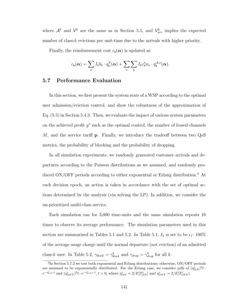
where Ak and Vk are the same as in Section 5.5, and Vkarr implies the expected

number of class-k evictions per unit-time due to the arrivals with higher priority.

Finally, the reimbursement cost cs(α) is updated as

cs(α) =∑

k

Ikbk · qVs (α) +∑

κ

∑

k

Ikcκkaκ · qA,κ

s (α).

5.7 Performance Evaluation

In this section, we first present the system state of a WSP according to the optimal

user admission/eviction control, and show the robustness of the approximation of

Eq. (5.5) in Section 5.4.3. Then, we evaluate the impact of various system parameters

on the achieved profit g∗ such as the optimal control, the number of leased channels

M , and the service tariff p. Finally, we introduce the tradeoff between two QoS

metrics, the probability of blocking and the probability of dropping.

In all simulation experiments, we randomly generated customer arrivals and de-

partures according to the Poisson distributions as we assumed, and randomly pro-

duced ON/OFF periods according to either exponential or Erlang distribution.3 At

each decision epoch, an action is taken in accordance with the set of optimal ac-

tions determined by the analysis (via solving the LP). In addition, we consider the

un-prioritized multi-class service.

Each simulation ran for 3,000 time-units and the same simulation repeats 10

times to observe its average performance. The simulation parameters used in this

section are summarized in Tables 5.1 and 5.2. In Table 5.1, Ik is set to be εI · 100%

of the average usage charge until the normal departure (not eviction) of an admitted

class-k user. In Table 5.2, γblock = γkblock and γdrop = γk

drop for all k.

3In Section 5.7.2 we test both exponential and Erlang distributions; otherwise, ON/OFF periodsare assumed to be exponentially distributed. For the Erlang case, we consider pdfs of (ηi

ON )2t ·e−ηi

ON ·t and (ηiOFF )2t · e−ηi

OF F ·t, t > 0, where ηiON = 2/E[T i

ON ] and ηiOFF = 2/E[T i

OFF ].

141

Channel C = 5, E[T iOFF ] = 10, E[T i

ON ] = 5, ∀iAuction pbid(M) = 0.7 ·M2

Customers Bk = k, µk = 1/7, ∀k,

λk(pk) = λmaxk e−pk , where (λmax

1 , λmax2 , λmax

3 ) = (5.5, 4.5, 5.5)

Eviction Ik = εI × pkBk/µk, εI = 0.5

Table 5.1: The list of common test parameters

Section M K γblock γdrop p

5.7.1 3 2 1.0 1.0 (1, 1.5)T

5.7.2 1-5 3 1.0 1.0 (1, 1.5, 2)T

5.7.3 1-5 3 1.0 1.0 (1, 1.5, 2)T

5.7.3 1-5 3 1.0 1.0 (1, 1.5, 2)T

5.7.3 3 2 1.0 1.0 0.5 ≤ p1, p2 ≤ 3.5

5.7.4 4 3 0.65-0.85 0.25-0.65 (1, 1.5, 2)T

Table 5.2: The list of test-specific parameters

5.7.1 System State Transition by Optimal Control

Fig. 5.6 illustrates the optimal actions derived by the proposed SMDP algorithm

in the form of state-transition diagram, when M = 3 and K = 2. For simplicity, the

state-transition diagram is drawn for m = 2 (i.e., when there are two idle channels)

and only the transitions by the user arrivals are presented. As shown, the optimal

admission policy deliberately rejects certain arrivals to maximize the profit, disabling

some possible state-transitions (shaded regions). It is also observed that the derived

optimal control is not threshold-type [67] as found in traditional networks with static

spectrum availability.

5.7.2 Approximation Accuracy of Eq. (5.5)

Fig. 5.7 shows the difference between the analytically-predicted results given by

Eq. (5.10) and the simulation results, for two different ON/OFF distributions: expo-

142

n1

n2

10 2 3 4 5 6 7 8 9 10

1

2

3

4

5

class 2

arrivals

class 1

arrivals

Figure 5.6: The state-transition diagrams of the proposed SMDP algorithm, accord-ing to user arrivals (shown for m = 2)

nential and Erlang. To focus on the accuracy of our analysis, we plot g∗ + pbid(M).

In Fig. 5.7(a), it is seen that the two results match well each other since there ex-

ists no approximation error in case ON/OFF periods are exponentially-distributed.

On the other hand, when ON/OFF periods are Erlang-distributed as in Fig. 5.7(b),

there exists only up to 4.4% difference between the simulated and analytic results

showing that the approximation in Eq. (5.5) produces reasonably accurate results.

The difference gets slightly larger as M grows due to the increase in the number of

channels where approximation is used.

5.7.3 Achieved Optimal Profit by SMDP Algorithm

We now show the optimal profit achieved by the proposed SMDP under various

test scenarios. We first compare the optimal profit of SMDP with the profit of the

simple complete-sharing (CS) algorithm [66], and show the impact of the system

parameters on the achieved profit such as the number of leased channels and the

service tariff.

143

1 2 3 4 50

5

10

15

20

# channels (M)g

* +

pb

id(M

)

SMDP (analysis)

SMDP (simulation)

(a) Exponential distribution

1 2 3 4 50

5

10

15

20

# channels (M)

g*

+ p

bid

(M)

SMDP (analysis)

SMDP (simulation)

(b) Erlang distribution

Figure 5.7: Approximation accuracy of Eq. (5.5) for two types of ON/OFF distribu-tions

Optimal vs. Non-optimal Control

We compare the performance of the proposed SMDP algorithm with the CS

algorithm in terms of g∗ and g∗ + pbid(M). The CS algorithm provides a simple

admission control that accepts any arrivals as long as there is room in the WSP’s

spectrum resources. Since CS is not designed to deal with eviction control, we

consider two possible variations of CS: CS with random eviction (denoted by ‘CS

+ Random’), and CS with optimal eviction control (denoted by ‘CS + EC’). At

channel vacation, ‘CS + Random’ chooses the users to evict one-by-one through

random selection, until the remaining users can fit in the available idle channels. On

144

1 2 3 4 5-6

-4

-2

0

2

4

# channels (M)

op

tim

al

pro

fit

(g*

)

SMDP

CS + EC

CS + Random

(a) optimal profit g∗

1 2 3 4 50

5

10

15

20

# channels (M)

g*

+ p

bid

(M)

SMDP

CS + EC

CS + Random

(b) g∗ + pbid(M)

Figure 5.8: Comparison of SMDP and two variations of CS in terms of their achievedprofits

the other hand, ‘CS + EC’ is derived by applying our SMDP procedure in Sections 5.4

and 5.5 by updating A1(s) in Eq. (5.3) as

A1(s) =

a : ak =

0 if (n + uk)TB > mC,

1 otherwise.

.

Fig. 5.8 shows that SMDP always achieves more profit than CS. In the tested

scenario, SMDP achieves up to 44% more profit than ‘CS + Random’ and up to 22.5%

more profit than ‘CS + EC’, in terms of g∗ + pbid(M).4 Comparison of ‘CS + EC’

4The reason why we consider g∗ + pbid(M) is to eliminate the effect of the bidding price for faircomparison, focusing on the profit achievement solely by the optimal control, since pbid(M) is givenand thus cannot be optimized.

145

and ‘CS + Random’ shows that the performance of CS is enhanced significantly by

employing the optimal eviction control. In addition, the performance gap between

the optimal SMDP and ‘CS + EC’ is much smaller than the gap between ‘CS +

EC’ and ‘CS + Random’, suggesting that eviction control makes more impact on

the achieved profit than the admission control does. It also shows that ‘CS + EC’

coincides with ‘CS + Random’ at M = 1 since there exists only one possible eviction

control at channel vacation (i.e., evict all users), and the performance gap between

two becomes more significant as M grows. This implies that the effect of eviction

control becomes dominant as the number of leased channels increases, due to the

time-varying spectrum availability.

Impact of Number of Leased Channels M

In Fig. 5.8(a), one can see that g∗ varies with M , having a peak value at M = 3.

This phenomenon stems from the tradeoff between the revenue generated by cus-

tomers (i.e., g∗ + pbid(M)) and the bidding cost (i.e., pbid(M)), because (1) a larger

M generates more revenue and less reimbursement cost due to more room available

to accommodate user arrivals, but (2) the gain will eventually be saturated due to

the bounded user population, and therefore, leasing more channels than necessary

becomes counter-productive, considering that pbid(M) grows faster than proportion-

ally to M as assumed in Section 5.3.2. Therefore, finding a proper M is essential

to profit maximization which can be achieved by determining and comparing g∗(M)

for various M using the proposed SMDP algorithm.

Impact of Service Tariff p

Due to the price-dependent arrival rate (i.e., λk(pk) = λmaxk e−pk), varying pk may

produce a different amount of profit. To show its impact on g∗, we evaluated the case

146

0.51

1.52

2.53

3.5

0.51

1.52

2.53

3.5-5

0

5

p1

p2

op

tim

al

pro

fit

(g*)

Figure 5.9: Optimal profit with various end-user pricing

of M = 3 and K = 2 while varying p such that 0.5 ≤ p1, p2 ≤ 3.50. Fig. 5.9 plots

the resulting g∗. It can be seen that as either p1 or p2 (or both) gets closer to 0.5

or 3.5, the resultant profit decreases dramatically due to the bounded user arrivals

by λmaxk (the case of 0.5) and decrease of the user arrival rate by e−pk (the case of

3.5), respectively. As a result, the profit function becomes concave, where the largest

profit can be attained at p = (2.0, 2.5). Therefore, a WSP must consider the impact

of its pricing policy on the overall profit, for which research on market demands and

customer statistics should be helpful to find the price–arrival rate relationship.

5.7.4 Tradeoffs between Two QoS Constraints

Fig. 5.10 plots the tradeoff between Pb and Pd. To show the relationship between

the two, we first fix γblock = 1.0 and vary γdrop in (a). Similarly, in (b), we fix

γdrop = 1.0 and vary γblock. As γdrop decreases, the QoS requirement on Pd becomes

stricter so that more in-service users may be protected from eviction at channel

vacation. For this, user arrivals must be blocked more often since the longer stay of

in-service users implies less idle resources for newly-arriving users. Thus, Pb increases

to compensate for the decrease of Pd which can be observed from Fig. 5.10(a) and (b),

147

0.25 0.3 0.35 0.4 0.45 0.5 0.55 0.6 0.650

0.1

0.2

0.3

0.4

0.5

0.6

0.7

0.8

0.9

1

γdrop

Pro

bab

ilit

y (

an

aly

sis)

Pb

1

Pb

2

Pb

3

Pd

1

Pd

2

Pd

3

(a) Varying γdrop

0.65 0.675 0.7 0.725 0.75 0.775 0.8 0.825 0.850

0.1

0.2

0.3

0.4

0.5

0.6

0.7

0.8

0.9

1

γblock

Pro

bab

ilit

y (

an

aly

sis)

Pb

1

Pb

2

Pb

3

Pd

1

Pd

2

Pd

3

(b) Varying γblock

Figure 5.10: The tradeoffs between Pb and Pd

more apparently at class 1. By contrast, as γblock decreases, the QoS requirement

on Pb becomes stricter so that less users may be rejected upon their arrival. To

accommodate more users, the WSP has to reserve more room by evicting more

users at channel vacation, thus increasing Pd. This phenomenon is clearly seen in

Fig. 5.10(b) at class 1.

148

5.8 Conclusion

In this chapter, we proposed the optimal admission and eviction control of CR

users to maximize a WSP’s profit at a CR hotspot. The problem was modeled

as an SMDP, and an LP algorithm was proposed to derive the optimal actions.

The two QoS constraints—user blocking and dropping probabilities—have also been

considered to strike a balance between profit maximization and user satisfaction. We

also introduced two types of prioritized user control to enable differentiated service

provisioning. The proposed LP algorithm is shown to outperform the CS algorithm,

and its sensitivity to the number of channels and the chosen pricing policy has been

studied.

149

CHAPTER VI

WHITESPACE UTILIZATION PART II: PRICE

AND QUALITY COMPETITION BETWEEN

CR SERVICE PROVIDERS

6.1 Introduction

The commercial use of dynamic spectrum access (DSA) has been encouraged

by the FCC’s ruling released in 2008 [28] that allows unlicensed radio operation in

the DTV bands by fixed and portable devices. The fixed devices represent high-

power stationary transceivers designed for the last-mile services in rural areas such

as IEEE 802.22 [1], and the portable devices represent short-range communication

devices in urban areas such as customer terminals for WiFi-like Internet access in

spectrum whitespaces (WS), often referred to as Wi-Fi 2.0 [3, 22, 52, 85]. Of these,

Wi-Fi 2.0 is considered as a promising commercial application of DSA with much

higher speed and less collision than today’s Wi-Fi using the ISM band, thanks to

the improved propagation characteristics of the WS such as larger coverage and the

wall-penetrating ability of the UHF/VHF bands [10].

The Wi-Fi 2.0 can be modeled as a three-tier dynamic spectrum market (DSM) [5]

consisting of three types of network entity: spectrum license holders, WSPs, and

cognitive radio (CR) customers, as illustrated in Fig. 6.1. The license holders can

150

End-Customers

(CR devices)

Wireless Service Providers

Wi-Fi like service

Spectrum Broker(Auctioneer)

Spectrum auction

Figure 6.1: The three-tier Wi-Fi 2.0 market

temporarily lease their spectrum to the WSPs via the multi-winner periodic spectrum

auction managed by the spectrum broker (SB). Once a WSP wins a channel at the

auction, it provides Internet access to the CR customers (or end-users) by utilizing

the leased spectrum, at popular public sites like coffee shops, libraries, or airports.

Once a leasing term ends, all channels are returned to the licensees and the WSPs

go through the auction again.

We employ the preemptive spectrum lease model in Chapter V. In this model,

when a WSP leases an ON/OFF channel, the primary users (PUs) of the channel

can preempt the leased channel for their own use during ON periods, thus restricting

the secondary users (SUs) to accessing only OFF periods as illustrated in Fig. 6.2.

Hence, the licensee collects the channel leasing fee only for the OFF periods. In fact,

this model is a realization of the private commons model in [5] which is considered

as a viable market option to benefit both PUs and SUs by enabling shared channel

access between PUs and SUs while making extra profit by leasing unused portions

of their spectrum.

In this chapter, we consider a duopoly Wi-Fi 2.0 network1 where two co-located

WSPs face price and quality competitions. Each WSP leases a licensed channel with

time-varying availability due to the ON-OFF channel usage patterns, and hence upon

1This chapter studies duopoly for the ease of analysis, but the duopoly scenario can still provideus enough insight into the network dynamics of Wi-Fi 2.0. In fact, the procedures introduced inSections 6.5 and 6.6 can be extended to the multi-WSP case, which is left as our future work.

151

appearance of PUs the WSP should evict all in-service customers from its network

(called channel vacation) to protect the PUs.2 We assume the WSP provides the

evicted customers with a monetary compensation by (partially) reimbursing their

service charges for the sake of customer satisfaction. Therefore, a WSP should lease

a channel with a proper quality in terms of channel utilization by PUs, that incurs less

eviction and smaller leasing cost. Each WSP should also determine the optimal price

strategy in terms of the service tariff, because a higher price than its competitor will

result in less customer arrivals and less profit according to the customers’ preference

on services. However, the price must be set high enough to be profitable, exceeding

the sum of the channel leasing and eviction costs.

6.1.1 Contributions

Our contribution in this chapter is three-fold. First, we model the interaction

between WSPs as a joint game with price and quality competitions while accounting

for time-varying spectrum availability. The existing game-theoretic approaches to

the dynamic spectrum market [23, 44, 46] have been limited to static idle channels,

and to the best of our knowledge, this is the first attempt to incorporate the effect of

time-varying channel availability in the game-theoretic framework. Next, we analyze

the market dynamics using a Markov chain and derive the Nash Equilibria (NE)

of the price and quality games. As to quality competition, we also discover the

market entry barrier for a WSP. Finally, we perform an extensive numerical analysis

to provide insightful results about the market dynamics of the Wi-Fi 2.0 network.

2Although the WSP can also keep customers in the system while suspending its service duringON periods, it cannot achieve seamless service provisioning.

152

ON

OFF

WSP leases a channel WSP returns the channel

(1) WSP utilizes only

OFF periods

(2) WSP is charged

leasing fee for

only OFF periods

…

Leasing period

Figure 6.2: The preemptive lease model with ON-OFF channels

6.1.2 Organization

The rest of the chapter is organized as follows. Section 6.2 briefly reviews related

work, and Section 6.3 introduces the system model and assumptions used in this

chapter. Section 6.4 models the problem as a Markov Chain and derives the profit

and cost functions. Then, Section 6.5 and Section 6.6 formulate and analyze the

price and quality competitions, respectively. The market dynamics under various

network conditions are shown via an extensive numerical analysis in Section 6.7, and

the chapter concludes with Section 6.8.

6.2 Related Work

Jia and Zhang [44] studied price and capacity competition in a duopoly DSA

market, assuming that the customer arrival rate is determined by a quadratic utility

function. However, it may not apply to our case where customers choose a service

based on price. Duan et al. [23] studied a similar problem with consideration to

physical-layer characteristics of heterogeneous end-users, and derived threshold-type

pricing rules. However, they assumed that the spectrum leasing cost is constant

and does not depend on the total demand in the spectrum auction. Kasbekar et

al. [46] considered a hierarchical game of quantity–price competition, with a two-

level prioritized service available to the end-users. None of the above-mentioned

153

work, however, considered time-varying spectrum availability, while assuming that a

leased channel is always idle during a leasing term.

6.3 System Model

In this section, we describe the system model and assumptions used throughput

the chapter.

6.3.1 Channel Model

We follow the channel model introduced in Chapter I. We also assume that WSP i

(i = 1, 2) leases a single channel with the capacity of Ci from the spectrum auction3

where each channel has exponentially distributed ON and OFF periods with rate

λONi and λOFF

i . Then, the channel utilization by PUs, denoted by ui,4 is given as

ui =1/λON

i

(1/λONi + 1/λOFF

i )=

λOFFi

(λONi + λOFF

i ).

Estimation of the channel parameters (i.e., λONi , λOFF

i , and ui) is possible via

spectrum sensing, as discussed in Chapter II. Detection of the ON/OFF patterns can

also be achieved via spectrum sensing, which has also been discussed in Chapters II,

III, and IV.

We assume homogeneous channel capacities such that Ci = C, ∀i, which would

be the case when the same type of licensed bands are considered (e.g., multiple DTV

channels).

3In this chapter, we use i as an index of a WSP and −i as an index of the competitor of WSPi, by slightly abusing the notation i which was previously reserved as channel index in Chapter I.However, this does not incur any ambiguity within the chapter since we only discuss single-channelWSPs.

4Note that this chapter uses ui instead of ui for the ease of notation.

154

6.3.2 Auction Model

We consider a multi-winner periodic spectrum auction [30, 97], where WSP i

leases a channel with the utilization of ui and pays the leasing fee of Li per unit-

time. To describe the form of Li, we introduce the concept of effective channel

capacity, denoted by Ceffi , given as

Ceffi = (1− ui)C,

which implies the total effective amount of leased spectrum available for WSP i.

Then, the DSA auction model in [44, 61] has shown that the unit price function

l, i.e., the leasing price per unit-bandwidth, is given as

l = γ1

(Ceff

i + Ceff−i

)γ2

, γ1 > 0, γ2 ≥ 1,

which is a positive, non-decreasing and convex function of (Ceffi + Ceff

−i ). That is,

the leasing cost depends on the total spectrum demand in the auction market, where

γ1 is the baseline cost when the total demand is unity. In addition, the leasing cost

increases faster than proportionally to the total demand (i.e., Ceffi +Ceff

−i ) due to the

competition between WSPs for the limited spectrum resources auctioned off, where

the degree of competition is described by γ2.

Finally, the leasing cost function Li of WSP i is given as

Li =Ceffi · l = γ1(1− ui)(2− ui − u−i)

γ2 , (6.1)

where γ1 = γ1C1+γ2 > 0 is the normalized γ1.

6.3.3 Service Model

Customer arrivals and departures

We assume that customer arrivals follow a Poisson distribution with rate λ and

their service time is exponentially distributed with mean 1/µ. We define ρ := λ/µ

155

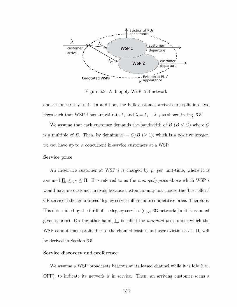
Co-located WSPs

customer

arrival

WSP 1

WSP 2

Eviction at PUs’appearance

Eviction at PUs’appearance

customer

departure

customer

departure

Figure 6.3: A duopoly Wi-Fi 2.0 network

and assume 0 < ρ < 1. In addition, the bulk customer arrivals are split into two

flows such that WSP i has arrival rate λi and λ = λi + λ−i as shown in Fig. 6.3.

We assume that each customer demands the bandwidth of B (B ≤ C) where C

is a multiple of B. Then, by defining α := C/B (≥ 1), which is a positive integer,

we can have up to α concurrent in-service customers at a WSP.

Service price

An in-service customer at WSP i is charged by pi per unit-time, where it is

assumed Πi ≤ pi ≤ Π. Π is referred to as the monopoly price above which WSP i

would have no customer arrivals because customers may not choose the ‘best-effort’

CR service if the ‘guaranteed’ legacy service offers more competitive price. Therefore,

Π is determined by the tariff of the legacy services (e.g., 3G networks) and is assumed

given a priori. On the other hand, Πi is called the marginal price under which the

WSP cannot make profit due to the channel leasing and user eviction cost. Πi will

be derived in Section 6.5.

Service discovery and preference

We assume a WSP broadcasts beacons at its leased channel while it is idle (i.e.,

OFF), to indicate its network is in service. Then, an arriving customer scans a

156

predetermined range of channels (e.g., a list of DTV channels reserved for Wi-Fi

2.0) to find in-service WSPs at its location, and selects the one advertising smallest

service price.5 In case the WSP chosen by the customer is fully occupied by SUs,

the customer is assumed to leave the Wi-Fi 2.0 site.6

When a WSP’s channel is occupied by PUs (i.e., ON), it cannot broadcast beacons

and no customer visits its network. Therefore, even if pi > p−i, WSP i can have

arrivals while WSP −i’s channel is busy. In summary, when pi > p−i, (1) λi = 0 and

λ−i = λ while WSP −i’s channel is idle, and (2) λi = λ and λ−i = 0 while WSP −i’s

channel is busy and WSP i’s channel is idle. In addition, when pi = p−i, we have

λi = λ−i = λ/2 while both WSPs have idle channels.

User eviction

At appearance of PUs, a WSP should evict all in-service customers from the net-

work to protect the PUs.7 Each evicted user is compensated by a reimbursement of

I, where I = β · pi/µ, β > 0, i.e., β times the average service charge of a normally

terminated session without eviction. We also assume β ≤ 1 to make the compen-

sation upper-bounded by what customers pay on average. In addition, we assume

λOFFi /µ = (1/µ)/

(1/λOFF

i

)< 1, because it is not beneficial to lease a channel that

cannot serve even a single session in an OFF period.

5One can consider other factors in service preference including QoS, data rate, and channelquality. In this chapter, we focus on the price as a sole factor.

6This is a reasonable assumption since the WSP-customer relationship is volatile due to theflexible design of CR devices [52]. That is, CR customers may choose different services (e.g., Wi-Fi,3G networks) by reconfiguring themselves if the desired WSP’s service is not instantly available.

7We assume the evicted customers will use alternative services such as Wi-Fi or 3G networks,due to the flexibility of the CR devices.

157

6.4 Two-Stage Market Competition

The market competition between WSPs can be modeled as a two-stage game,

consisting of price and quality games. The quality game is performed periodically

at every auction, where each WSP competes for the desired quality of spectrum

resources to lease, in terms of ui. The quality game is a one-shot game, and thus a

WSP cannot return or change the leased channel during a leasing term. During a

leasing term, two WSPs perform a price competition to determine the optimal price

pi for their maximal profit. The quality game is also called a full -game in the sense

that the optimal quality of spectrum is determined by assuming the NE prices of the

two WSPs achieved at a price sub-game.

As the main objective of a WSP is to maximize its profit, the profit function

must be analytically derived before investigating the price and quality competition.

To derive the profit, we define the system state of WSP i as si = (mi, ni) where mi

is the channel state such that

mi =

0 if channel is busy,

1 if channel is idle,

and ni is the number of in-service customers with ni ∈ [0,miα]. Then, the system

state transition can be modeled as a Markov Chain under the assumption of Poisson

arrivals, exponential service times, and exponential ON and OFF periods.

Fig. 6.4 illustrates the state-transition diagram of the Markov Chain. The hor-

izontal transitions represent the state transitions by the customer arrivals and de-

partures, and the vertical transitions represent the state transitions due to ON-OFF

channel state changes. A customer arrival is accepted by the system if ni < miα.

When an idle channel becomes busy, all ni customers are evicted from the system.

158

1, 11, 0 1,

0, 0

iλ

µ 2µ

ON

iλ OFF

iλ …

System state = (mi , n

i)

mi: channel state (0 or 1)

ni: number of in-service customers

ααµ

idle

busy

1, 2

3µ

…

OFF

iλ OFF

iλOFF

iλ

iλ

iλ

iλ

Figure 6.4: State transition of WSP i’s system

From Fig. 6.4, we first notice that

π0,0 = ui,α∑

ni=0

π1,ni= 1− ui,

where πsi= πmi,ni

denotes the stationary distribution of the system. Then, the

global balance equations can be derived in a matrix form as follows.

A

(π1,0 π1,1 . . . π1,α

)T

=

(u · λON

i

µ0 . . . 0

)T

, (6.2)

where

A =

f(0) −1 0 0 . . . 0 0 0

−ρi f(1) −2 0 . . . 0 0 0

0 −ρi f(2) −3 . . . 0 0 0

. . . . . . . . . . . . . . . . . . . . . . . . . . . . . . . . . . . . . . . . . . . . . . . . . . . . .

0 0 0 0 . . . −ρi f(α− 1) −α

0 0 0 0 . . . 0 −ρi f(α)− ρi

,

by defining f(k) := ρi + λOFFi /µ + k and ρi := λi/µ. Therefore, using Eq.(6.2) the

stationary probability is found as

(π1,0 π1,1 . . . π1,α

)T

= A−1

(u · λON

i

µ0 . . . 0

)T

.

159

Although a numerical analysis can be used to find A−1, the stationary probability

in a closed-form is preferred in analyzing the price and quality games to obtain

an insight in the form of the price and quality NEs. Therefore, we approximate

the original Markov Chain by applying a state decomposition technique introduced

in [33].

According to [33], we can group the states in Fig. 6.4 with the same mi (i.e., the

states in the same row) together as long as the vertical state-transition rates are much

smaller than the horizontal state-transition rates. In DSA, this condition is expected

to be met in many applications because spectrum reuse is intended for under-utilized

channels with relatively longer ON/OFF periods (e.g., TV bands) compared to the

customer arrival/departure by the SUs. In Section 6.7, we will quantify the impact

of this approximation on the accuracy of the analysis through extensive numerical

experiments.

After the decomposition, the system becomes M/M/α/α while the channel is

idle. Hence, we can express πsias

πsi≈ πni|mi

· P (mi) =

ui if si = (0, 0),

πni· (1− ui) if mi = 1.

where πniis the stationary probability of a M/M/α/α system such that

πni(ρi) =

(ρi)ni/ni!∑α

n=0 (ρi)n/n!, ∀ni. (6.3)

Then, revenue and eviction cost occurs only when channel is idle because ni = 0

for a busy channel. Hence, for mi = 1, we derive the revenue rate R(pi, ρi) (the

160

average revenue per unit time) and the eviction cost E(pi, ρi) as follows:

R(pi, ρi) =α∑

ni=0

pini · πni(ρi) = piρi

∑α−1n=0 (ρi)

n/n!∑αn=0 (ρi)n/n!

E(pi, ρi) =α∑

ni=0

Ini · πni(ρi) · λOFF

i = βλOFF

i

µR(pi, ρi)

where λOFFi is the transition probability due to the OFF→ON transition of an idle

channel.

The derived R(pi, ρi) and E(pi, ρi) will become our bases in the later sections to

calculate the profit rate of WSP i under the various market conditions. For the ease

of notation, we define

∆(pi, ρi) := R(pi, ρi)− E(pi, ρi).

6.5 Price Competition Analysis

In this section, we investigate a price competition sub-game to find the best tariff

strategy of WSP i in terms of pi, when (ui, u−i) are given. We also study the necessary

condition for the existence of the price NE and derive the NE at such conditions.

The derived price NE will be applied to the quality full-game in Section 6.6, in

determining the profit at the equilibrium price for a given set of quality.

6.5.1 Three Pricing Strategies

At WSP i, the price of the competitor WSP −i (i.e., p−i) is known since the

WSP −i advertises its tariff via the beacons. Then, the WSP i can take one of the

following three pricing strategies according to the relationship between pi and p−i:

(1) pi < p−i, (2) pi > p−i, and (3) pi = p−i. We overview each strategy to derive the

conditional profit of WSP i.

161

• Under strategy 1 (pi < p−i): WSP i can monopolize the market and hence its

profit is maximized at pi = p−i − ε, ε > 0, where ε can be arbitrarily small. In this

case, the profit rate of WSP i becomes

F{pi<p−i}i = (1− ui) ·∆(p−i − ε, ρ)− Li. (6.4)

• Under strategy 2 (pi > p−i): WSP i loses the entire market to its competitor

(i.e., λi = 0 and λ−i = λ) if WSP −i has an idle channel (i.e., m−i = 1). On the

contrary, while m−i = 0, it becomes λi = λ and λ−i = 0 if WSP i’s channel is idle.

Therefore, with probability u−i ·(1−ui), the stationary probability of WSP i’s system

follows Eq. (6.3). In this case, WSP i’s profit is maximized at pi = Π since WSP −i

is out-of-service, and thus WSP i’s profit rate is given as

F{pi>p−i}i = (1− ui)u−i ·∆(Π, ρ)− Li. (6.5)

• Under strategy 3 (pi = p−i): Here, we need to consider two cases. First, when

mi = m−i = 1, two WSPs take an equal share of the market such that λi = λ−i =

λ/2. Second, when mi = 1 and m−i = 0, we have λi = λ and λ−i = 0 since the

arriving customers cannot find the service beacons of WSP −i. Therefore, by setting

pi = p−i, the profit rate of WSP i becomes

F{pi=p−i}i =(1− ui)

{u−i ·∆(p−i, ρ) + (1− u−i) ·∆(p−i,

ρ

2)}− Li. (6.6)

6.5.2 Optimal Price Strategy

The goal of WSP i is to maximize its profit by optimally determining its price pi

for a given p−i. Hence, we will compare the profit rates of the three pricing strategies

in Section 6.5.1 to derive the optimal pi.

162

p1

p2

p1(p2)

p2(p1) p1=p2

Π

2∏

1∏ Π

1u

Π2u

Π

No NE

exists!ε

(a) Π1 ≤ u1Π, Π2 ≤ u2Π

p1

p2 p1=p2p2(p1)

p1(p2)

No NE

exists!2∏

Π

Π1∏

ε

Π1u

Π2u

(b) Π1 ≤ u1Π, Π2 > u2Π

p1

p2

NE =

p1=p2

Π1∏

2∏

Π

p2(p1)

p1(p2)

( )2 2

,∏− ∏ ε

ε

Π2u

Π1u

(c) Π1 > u1Π, Π2 > u2Π

Figure 6.5: Nash Equilibrium of the price competition

Comparison of price strategies 1 and 3

We first compare strategies 1 and 3 in terms of their profit rates given by Eqs. (6.4)

and (6.6) as follows (when ε → 0+):

F{pi<p−i}i − F

{pi=p−i}i = (1− ui)(1− u−i)p−i

(1− β

λOFFi

µ

)Ar (6.7)

where

Ar := ρ

{∑α−1n=0 ρn/n!∑αn=0 ρn/n!

− 1

2·∑α−1

n=0 (ρ/2)n/n!∑αn=0 (ρ/2)n/n!

}.

163

Lemma 6.5.1. For 0 < ρ < 1 and α ≥ 1, Ar > 0.

Proof. See Appendix A.

Theorem 6.5.1. Price strategy 3 (pi = p−i) is strictly dominated by price strategy

1 (pi < p−i).

Proof. In Eq.(6.7),(1− βλOFF

i /µ)

> 0 since β ≤ 1 and λOFFi /µ < 1 by our assump-

tion, and Ar > 0 by Lemma 6.5.1. Therefore, we have F{pi<p−i}i > F

{pi=p−i}i , ∀p−i,

which completes the proof.

Comparison of price strategies 1 and 2

Next, we compare strategies 1 and 2 in terms of their profit rates given by

Eqs. (6.4) and (6.5) as follows (when ε → 0+):

F{pi<p−i}i − F

{pi>p−i}i = (1− ui) (p−i − u−iΠ)

(1− β

λOFFi

µ

)ρ

∑α−1n=0 ρn/n!∑α

n=0 ρn/n!. (6.8)

Theorem 6.5.2. The optimal price strategy is

• Strategy 1 (pi = p−i − ε), if p−i > u−i · Π,

• Strategy 2 (pi = Π), if p−i ≤ u−i · Π.

Proof. By Theorem 6.5.1, price strategy 3 cannot be optimal. Hence, we only need

to compare strategies 1 and 2. In the proof of Theorem 6.5.1, it has been shown that

(1− βλOFF

i /µ)

> 0. Therefore, by considering the form of Eq. (6.8), it is seen that

strategy 1 is optimal (i.e., F{pi<p−i}i > F

{pi>p−i}i ) if p−i > u−i · Π; otherwise strategy

2 is optimal.

164

6.5.3 Nash Equilibrium of the Price Competition

Using the derived optimal price strategy, we can find the Nash Equilibrium of

the price competition. We first describe how to determined the marginal price for

each WSP, and then derive the NE and its existence condition.

Finding the Marginal Price

We define the marginal price Πi as the minimal price to guarantee a non-negative

profit for WSP i even at the worst case. That is, when pi = Πi, the WSP i should

be able to achieve at least a break-even (zero profit) regardless of p−i.

When we fix pi = Πi, the profit rate Fi previously given as Eqs. (6.4),(6.5),(6.6)

becomes

• F{pi<p−i}i = (1− ui) ·∆(Πi, ρ)− Li,

• F{pi>p−i}i = (1− ui) · u−i∆(Πi, ρ)− Li,

• F{pi=p−i}i = (1− ui)

{u−i∆(Πi, ρ) + (1− u−i)∆(Πi,

ρ2)}− Li.

It can be observed that F{pi>p−i}i is the worst. Therefore, to guarantee Fi ≥ 0,

we need to set

Πi =Li/u−i

(1− ui) ·∆(Πi, ρ)/Πi

=Li/u−i

(1− ui)χi(ρ)=

γ1(2− ui − u−i)γ2

u−iχi(ρ), (6.9)

where Eq.(6.1) is applied. Here, χi(ρi) is defined as

χi(ρi) :=

(1− β

λiOFF

µ

)ρi

∑α−1n=0 (ρi)

n/n!∑αn=0 (ρi)n/n!

. (6.10)

Note that if the determined Πi satisfies Πi > Π, WSP i cannot make positive

profit for any pi since λi = 0 for pi > Π making the profit strictly negative such as

Fi = −Li. Therefore, WSP i should opt out of the market when Πi > Π in order not

to incur any channel leasing cost. In the next section, this will be modeled as forcing

165

ui = 1 at the quality competition where the channel leasing cost becomes zero since

Ceffi = 0.

Finding the Nash Equilibrium

To find the NE, we consider the case where Πi ≤ Π and Π−i ≤ Π so that both

WSPs may participate in the market competition. Fig. 6.5 shows the NE of the price

competition, where the solid plot represents p1(p2), i.e., the best response function of

WSP 1 given p2, and the dashed plot represents p2(p1). The best response functions

are drawn by following the optimal strategy in Theorem 6.5.2. Note that WSP i

never decreases its price pi smaller than Πi, and hence pi(p−i) is lower-bounded by

Πi.

It can be seen from Figs. 6.5(a),(b) that there exists no NE when (1) Πi ≤ uiΠ

and Π−i ≤ u−iΠ, or (2) Πi ≤ uiΠ and Π−i > u−iΠ, since p1(p2) and p2(p1) never

intersect with each other.

As shown in Fig. 6.5(c), the NE exists when Πi > uiΠ and Π−i > u−iΠ, where

the NE is given as (Π2 − ε, Π2) for Π2 > Π1. Due to symmetry, the NE becomes

(Π1, Π1 − ε) for Π1 > Π2. Therefore, as ε → 0, there exist a unique NE described as

follows in Theorem 6.5.3.

Theorem 6.5.3. The NE of the price competition exists only when Πi > uiΠ and

Π−i > u−iΠ, and the unique NE is determined as (p1, p2) = (p∗, p∗), where p∗ =

max{Π1, Π2} and Πi is given as in Eq.(6.9).

6.6 Quality Competition Analysis

The goal of the quality competition is to find the best channel to lease with

optimal quality in terms of ui that achieves maximal profit of WSP i at the equi-

166

librium price found in Section 6.5. Having the NE of the price competition as

pi = p−i = max{Π1, Π2}, the resulting profit of WSPs is given as Eq. (6.6), and

we want to find the best response function ui(u−i) to maximize such profit.

As introduced in the channel model, ui = λOFFi /(λOFF

i + λONi ), and thus there

exist infinitely many possible pairs of (λOFFi , λON

i ) for a given ui. Therefore, we

would like to consider a scenario where λOFFi = λOFF ,∀i, representing the case

when channels have identically distributed intervals between PU activities. It is also

possible to consider another scenario where λONi = λON ,∀i (i.e., the duration of PU

activities follows the same distribution over channels), which is left as our future

work.

Note that even though the optimal ui can be found for any γ2 ≥ 1, we are

particularly interested in the case of γ2 = 1 as an illustrative example.

6.6.1 Market entry barrier

WSP i’s profit becomes strictly negative in case its marginal price becomes greater

than the monopoly price (i.e., Πi > Π), because there will be no customer arrival

while the channel leasing fee must be still paid. If this happens, the WSP would

rather shut down its service by leasing no channel (equivalently, leasing a channel

with ui = 1). Therefore, there exists a market entry condition for a WSP, which is

described by Πi ≤ Π. For a given u−i, this condition results in the following interval

of ui:

2−(

1 +Πχi(ρ)

γ1

)u−i ≤ ui. (6.11)

In addition, the same claim applies to WSP −i by switching the role of i and −i.

167

1

u1

u2

uA

1

20

2uA

2

2uA

21 uu =

2

1

11 )

)(1(2 uu

γ

ρχΠ+−=

)2()(

))(

1(2 2

21

111

1

22 uuuu −

Π+=⇔

Π+−=

ρχγ

γ

γ

ρχ

Region I

Region II

Region

III

Region

IV

Region

V

uB

uB

Figure 6.6: Five decision regions of (u1, u2)

6.6.2 Region-specific optimal quality strategies

According to the market entry points of the two WSPs, we can divide the area

of (u1, u2) into five regions as shown in Fig. 6.6.

Region I and II (below the market entry barrier)

The region I is a rectangular area where 0 ≤ ui ≤ 1 and 0 ≤ u−i < uA. The

region represents the case when WSP i cannot overcome the market entry barrier

and it leaves the market. Therefore, the best response function in u−i ∈ [0, uA) is

ui(u−i) = 1.

The region II, that does not include the line ui = 2 − (1 + Πχi(ρ)/γ1

)u−i, also

belongs to the case when WSP i cannot overcome the market entry barrier. However,

the region does not include ui = 1, and hence no possible solution exists. As a result,

we can ignore this region in deriving ui(u−i).

168

Region III (a monopoly market)

The region III includes the line 2 − (1 + Πχi(ρ)/γ1

)u−i = ui, but excludes the

line u−i = 2 − (1 + Πχ−i(ρ)/γ1

)ui. Therefore, p−i > Π in the region due to the

market entry condition, and thus WSP −i will not have any customer arrival. As a

result, WSP i monopolizes the market with pi = Π. With the monopoly price, WSP

i’s profit rate becomes

F IIIi =(1− ui)×

{Πχi(ρ)− γ1(2− u−i − ui)

}(6.12)

Region IV (a duopoly market)

In the region IV, both WSPs can enter the market, and satisfy the condition

ui ≤ u−i where we have Πi ≤ Π−i. Therefore, the NE price becomes p∗ = Π−i and

WSP i’s profit rate becomes

F IVi =(1− ui)× {(u−iχi(ρ) + (1− u−i)χi(ρ/2)) p∗ − γ1(2− u−i − ui)}

=γ1(1− ui)(2− u−i − ui) (ψ − ui) · 1

ui

,

(6.13)

where ψ = u−i + (1 − u−i)χi(ρ/2)/χ−i(ρ). For ui ∈[

γ1

γ1+Πχ−i(ρ)(2− u−i), u−i

],

Eq. (6.13) is maximized at ui = γ1

γ1+Πχ−i(ρ)(2 − u−i), because Fi → ∞ as ui → 0

and u−i ≤ ψ < 1 ≤ (2− u−i) where ψ < 1 is given by Lemma 6.5.1.

Region V (a duopoly market)

Similar to the region IV, the region V also belongs to the duopoly market. As

seen, the region satisfies the condition ui ≥ u−i where we have Πi ≥ Π−i. Therefore,

the NE price becomes p∗ = Πi, and WSP i’s profit rate becomes

F Vi = (ui − 1)(ui + u−i − 2) · γ1(1− u−i)χi(ρ/2)

u−iχi(ρ). (6.14)

169

Then, due to the form of the region V, two distinct cases are considered. First, for

u−i ∈ [uA, uB), we have 0 < 2− (1 + Πχi(ρ)/γ1

)u−i ≤ ui ≤ 1. Since 1 ≤ (2− u−i),

Eq. (6.14) is maximized at ui = 2− (1 + Πχi(ρ)/γ1

)u−i.

Next, for u−i ∈ [uB, 1], we have ui ∈ [u−i, 1], and thus Eq. (6.14) is maximized at

ui = u−i.

6.6.3 Optimal quality strategy

Finally, we derive the optimal quality strategy, i.e., the best response function

ui(u−i) for all possible intervals of u−i. As already shown, the best response function

in u−i ∈ [0, uA) is ui(u−i) = 1. For u−i ∈ [uA, uB), we compare the regions II and V,

but as pointed out earlier, we can ignore the region II. Therefore, the best response

function in u−i ∈ [uA, uB) is ui(u−i) = 2− (1 + Πχi(ρ)/γ1

)u−i.

For u−i ∈ [uB, 1], we need to compare all three regions (III, IV, and V) in order

to determine the best response function. First, it can be easily shown that the

best profit in the region V cannot exceed the best profit of the region IV for the

following reason. The maximal profit of the region V for u−i ∈ [uB, 1] is achieved at

ui = u−i, which is a shared line with region IV. However, ui = u−i does not provide

the maximal profit in the region IV, and thus the maximal profit of the region IV is

larger than that of the region V.

Next, for given u−i, let uIVi denote the optimal ui in the region IV such as

uIVi = γ1

γ1+Πχ−i(ρ)(2 − u−i). Let us also consider ui = uIV

i − ε, ε > 0, which is in the

region III. If we compare Eq. (6.13) at ui = uIVi and Eq. (6.12) at ui = uIV

i − ε for

an arbitrarily small ε, then we can easily observe that the leasing cost is arbitrarily

close to each other in both regions while Πχi(ρ) > (u−iχi(ρ) + (1− u−i)χi(ρ/2)) Π−i.

Therefore, we can conclude that the best profit in the region IV cannot exceed the

170

1u1

u2

1

0

21uu =

u1(u2)

u2(u1)

uA

2uA

uB

2uAuB

NE = (uB, uB)

Figure 6.7: The Nash Equilibrium of the quality competition

profit in the region III at ui = uIVi − ε, and thus the best response function exists in

the region III.

Fig. 6.7 plots the resulting best response ui(u−i) for u−i ∈ [0, 1], where u−i(ui)

is also drawn using the symmetry. It is observed that, regardless of the optimal ui

in the region III, there exists a NE of the quality game at (uB, uB) where uB is an

intersection of ui = u−i and ui = 2−(1 + Πχi(ρ)/γ1

)u−i, resulting in Theorem 6.6.1

as follows.

Theorem 6.6.1. The NE of the quality competition exists at (u1, u2) = (u∗, u∗),

where u∗ = 2γ1/{2γ1 + Πχ1(ρ)}.

Note that there exist two additional NEs other than (u1, u2) = (u∗, u∗): (u, 1)

and (1, u), where 0 ≤ u < uA. However, according to the concept of the focal point

introduced in [23,59], these NEs are not likely to be chosen by the WSPs since such

NEs exclude either WSP from the market thus impairing the fairness.

From Theorem 6.6.1, we obtain the following two corollaries.

171

Corollary 6.6.1. At the NE of the quality competition, the NE price becomes p∗ = Π.

Proof. By applying ui = u−i = u∗ to Eq. (6.9), we obtain Πi = Π since χ1(ρ) = χ2(ρ).

Therefore, p∗ = Π by Theorem 6.5.3.

Corollary 6.6.2. The NE of the quality competition satisfies the equilibrium price

existence condition.

Proof. Since Πi = Π, we have Πi > uiΠ and Π−i > u−iΠ for ui = u−i = u∗ 6= 1.

6.6.4 Discussion

WSPs may, in reality, not be able to find the channel that exactly matches their

needs, whose utilization factor equals u∗. In such a case, they should make a reason-

able assumption that both WSPs would act rationally to bid for the best matching

channel whose utilization factor is closest to u∗. This strategy is reasonable in that

the quality competition is a one-shot game performed once at each periodic auction,

and thus a WSP cannot make any adjustment on its leased channel until the next

auction.

In case u takes its value from a countable set in a discrete manner, the quality

competition becomes a combinatorial matching problem that should consider all

possible pairs of (u1, u2) from the given channel set. The problem formulation in

such a case becomes quite different from the procedure presented in this chapter, as

the best response function is no more continuous. We leave the case as our future

work.

The quality competition problem can be further extended to a joint quantity/quality

competition when we consider WSPs, each operating with multiple channels. That

172

is, WSP i leases more than one channel, say Mi channels, and combine them into a

one logical channel with a larger capacity (e.g., Mi · C). In such a case, we need to

find the best quantity/quality pair of (Mi, ui),8 for a given pair of (M−i, u−i). Hence,

the decision space becomes N × [0, 1] where N is a set of natural numbers, with

additional complexity coming from the choice of Mi. We also leave such extension

as our future work.

6.7 Evaluation of Wi-Fi 2.0 Network Dynamics

We now conduct an extensive numerical analysis to provide insight into the mar-

ket dynamics of the Wi-Fi 2.0 network. First, we compare the profit observed from

a simulated scenario with the analytically-derived profit to investigate the condition

under which our state decomposition approach can be applied with a tolerable ap-

proximation error. Next, we study the fundamental tradeoffs between the network

parameters at equilibrium, including the arrival rate λ, the leasing cost γ1, and the

eviction cost β.

In each scenario, we set a list of common parameters as follows: C = 5, B = 1,

and γ2 = 1.

6.7.1 Approximation accuracy in state decomposition

We compare the profit observed from the simulation with the profit given by the

analysis to derive the condition under which state decomposition performs reasonably

well. In the simulation, we randomly generate 200 pairs of exponential ON and

OFF periods and also emulate user arrivals and departures. A simulation is run by

applying the optimal price and quality found by the analysis, and repeats 10 times

to derive the average performance. Other simulation parameters are set as Π = 2,

8Assuming all Mi channels are of the same quality ui.

173

0 0.05 0.1 0.15 0.20

0.2

0.4

0.6

0.8

λOFF

/µ

Profit

AnalysisS imulation

Figure 6.8: Decomposition approximation accuracy

ρ = 0.9, γ1 = 0.1, and β = 0.25.

From Fig. 6.8, one can see that the profit predicted by analysis gets fairly close to

the actual achieved profit at a small λOFF /µ, and the gap between them gradually

increases as λOFF /µ grows. At λOFF /µ = 0.1, the approximation error is found

to be less than 9.5%, which becomes around 15% at λOFF /µ = 0.15. In case the

tolerable error is less than 10%, the state decomposition approach is effective for

λOFF /µ ≤ 0.1, implying that an OFF period, on average, can accommodate at

least 10 consecutive user sessions. Note that this is a plausible scenario since DSA

targets to reuse under-utilized channels with relatively larger ON/OFF periods than

customer arrivals/departures.

6.7.2 Impact of arrival rate and leasing cost

In Fig. 6.9(a), we plot the achieved profit of a WSP at its equilibrium while

varying the arrival rate λ (equivalently ρ). The leasing cost is also varied by testing

three selected values of γ1. In this test, the simulation parameters are set as Π = 1,

174

µ = 1/5, λOFF = 1/500, λON = 1/50, and β = 0.25. It can be seen that as

the arrival rate increases (i.e., ρ → 1), the WSP achieves more profit due to the

increased revenue. The profit also enhances as γ1 decreases, due to the less leasing

cost by Li.

In Fig. 6.9(b), we also plot the quality equilibrium u∗ under the same test condi-

tions. As the arrival rate increases, u∗ is monotonically decreasing because the WSP

can overcome the leasing cost by accommodating more customers using a less busy

channel (i.e., smaller u∗). Therefore, when ρ → 0, the best strategy is to leave the

market by setting u∗ = 1. On the other hand, at the same ρ, u∗ increases as γ1

increases, because it can compensate the increased leasing cost by leasing a less idle

channel.

6.7.3 Impact of eviction cost

In Fig. 6.9(c), we plot the achieved profit at equilibrium versus the average OFF

period (i.e., 1/λOFF ) under the various eviction costs given by β. Other simulation

parameters are set as Π = 1, ρ = 0.9, γ1 = 0.3, and λON = 1/50.

At the same 1/λOFF , a larger profit is achieved at a smaller β due to the amount of

reimbursement to the evicted users, and the difference becomes more pronounced as

1/λOFF decreases. This implies that eviction becomes more dominant in a dynamic

channel environment (i.e., channels with small ON and OFF periods) than in a static

environment, due to more frequent evictions.

6.8 Conclusion

In this chapter, we studied the competition between WSPs in the duopoly Wi-Fi

2.0 network while considering time-varying spectrum availability. We modeled the

problem as a joint price and quality game where two co-located WSPs compete for

175

leasing limited spectrum resources and enticing customers to their service. A WSP’s

profit function is derived by considering the dependency of revenue on the pricing

policy, the eviction cost due to the reimbursement of the evicted customers, and the

channel leasing cost. It is shown that the price game has a unique NE at a larger

marginal price of the two WSPs, and the quality game has a NE that balances the

marginal price with the monopoly price. Using an extensive numerical analysis, we

have demonstrated the fundamental tradeoffs in the Wi-Fi 2.0 network due to the

factors, such as customer arrival rate, channel dynamics, and eviction cost.

176

0 0.2 0.4 0.6 0.8 10

0.05

0.1

0.15

0.2

0.25

0.3

0.35

Profit

ρ

γ1=0.1

γ1=0.2

γ1=0.3

(a) Profit Fi vs. arrival rate λ

0 0.2 0.4 0.6 0.8 10

0.2

0.4

0.6

0.8

1

u*

ρ

γ1=0.1

γ1=0.2

γ1=0.3

(b) Quality NE u∗ vs. arrival rate λ

101

102

103

0.1

0.15

0.2

0.25

0.3

0.35

1/λOFF

Profit

β=0.0

β=0.25

β=0.5

β=0.75

β=1

(c) Profit Fi vs. eviction cost β

Figure 6.9: Fundamental tradeoffs in the duopoly market

177

CHAPTER VII

Conclusion and Future Direction

This dissertation addresses the issues of efficient discovery and utilization of spec-

trum opportunities to better integrate the dynamic spectrum access (DSA) mecha-

nism into the current wireless networking paradigm. This chapter summarizes our

contributions and presents possible future research directions.

7.1 Research Contributions

The major contributions of this research are grouped into two categories: effi-

cient opportunity discovery and efficient opportunity utilization. In particular, we

addresses opportunity discovery in the context of spectrum sensing of in-band and

out-of-band channels, and addresses opportunity utilization in the application of

Wi-Fi-like whitespace utilization.

7.1.1 Contributions in Opportunity Discovery

The success of DSA hinges on how to strike a balance between the following two

conflicting objectives: (1) to efficiently discover opportunities with minimal sensing

overhead, and (2) to protect PUs against harmful interference from SUs. We ad-

dressed this issue by proposing two types of out-of-band sensing techniques and an

in-band sensing scheme.

178

In Chapter II, we consider a bandwidth-craving CR network (CRN) which aims

to discover as much opportunities as possible from out-of-band channels to achieve a

higher throughput. We propose a periodic out-of-band sensing scheme that optimizes

sensing-periods of multiple out-of-band channels to maximize the utilizable portion

of opportunities. The utilizable opportunity implies the portion of opportunities

discovered by out-of-band sensing which are uninterrupted by out-of-band sensing of

other channels in case a sensor and a transceiver are co-located at each SU.

In Chapter III, we consider a bandwidth-limited CRN which seeks a specific

amount of bandwidth determined as the sum of spectrum demands from all SUs in

the CRN. In such a setup, we focus on the case where channel vacation incurs a

shortage of spectrum opportunities and triggers reactive out-of-band sensing to find

additional spectrum opportunities to compensate for the loss of bandwidth due to

the channel vacation. We propose an optimal sequence of out-of-band channels that

minimizes the delay in finding the necessary amount of opportunities to promote

seamless service provisioning. The optimal sensing sequence is derived by dynamic

programming (DP) with consideration of the heterogeneous channel characteristics,

and a near-optimal sequencing algorithm is also proposed which reduces the compu-

tational complexity of DP by finding the suboptimal sequence in polynomial-time.

In Chapter IV, we study PU protection via periodic in-band sensing with an

objective of detecting returning PUs at in-band channels within a hard deadline

determined by the FCC requirement. Especially, we optimally schedule periodic in-

band sensing by deriving optimal sensing-time and sensing-period incurring minimal

sensing overhead while achieving all the PU detection requirements such as sensing

latency, sensitivity, and accuracy. We also identify a tradeoff between energy and

feature detection and compare the two schemes to determine a better detection

179

method in terms of sensing overhead according to the varying sensing environments.

7.1.2 Contributions in Opportunity Utilization

The discovered spectrum opportunities should be utilized in a way that SUs can

benefit from DSA and the legacy spectrum can be used more efficiently. We focus

on Wi-Fi-like whitespace applications where SUs can access the Internet via DSA-

enabled access points (called CR hotspot) operated by the secondary wireless service

providers (WSPs). Such applications may appear in early stages of DSA deployment

due to its popularity in the current consumer market. In this context, we address two

issues in the problem of WSP’s profit maximization: (1) CR customer flow control

at each CR hotspot, and (2) competition between co-located WSPs.

In Chapter V, we propose an optimal admission and eviction control of CR users

at CR hotspots where a multi-class service is provided and spectrum availability is

time-varying due to the ON/OFF channel usage patterns by PUs. We address the

issues in the dynamic spectrum market (DSM) where the license holders lease their

own spectrum to WSPs via dynamic spectrum auction. According to the system

state in terms of the number of in-service customers, the arriving customers are

either admitted or rejected, and at channel vacation in-service customers are selec-

tively evicted from the service to fit into the remaining spectrum opportunities. The

optimization problem is modeled as a semi-Markov decision process (SMDP) and a

linear programming (LP) algorithm is formulated to derive the optimal control.

In Chapter VI, we consider price and quality competition between co-located

WSPs where they compete for leasing the spectrum with the best quality at spectrum

auction and for enticing more customers by providing more competitive pricing. The

problem is modeled as a duopoly game and the Nash Equilibria of the service tariff

180

and the quality of the leased channel are derived.

7.2 Future Direction

This section describes possible future research directions related to the efficient

integration of DSA into the future wireless networks.

7.2.1 Energy-efficient Spectrum-agile Networking

Although DSA may help support better quality-of-service (QoS) in wireless com-

munications, the cost in deploying and managing CR sensors must be taken into

account. Among the various issues in CR sensor management, energy efficiency is

an interesting issue which can be addressed as follows. First, an efficient sensing al-

gorithm needs to be developed to choose the best sensors to collaborate according to

the sensors’ heterogeneous lifetime distribution and their surrounding environments

(e.g., fading). Next, to enhance the lifetime of each sensor, the sensing algorithm

should be able to mitigate sensing overhead, radio reconfiguration time, and sensing

report dissemination time. Finally, when there are multimedia users competing for a

limited spectrum resource, a dynamic resource sharing algorithm can be developed to

derive an optimal sharing strategy with minimal collision and contention, for which

game theory can be adopted.

7.2.2 Coexistence of Heterogeneous Wireless Networks

Due to the exponential growth of wireless services, coexistence of heterogeneous

networks has become a serious issue. CR techniques may help mitigate such prob-

lems, since CR networks are inherently required to coexist with legacy systems. In

the context of coexistence, “spectrum etiquette” implies a scheme that describes

how collocated networks can share spectrum resources through resource negotiation,

181

renting, and contention. Therefore, we can extend the spectrum etiquette concept

for coexistence of the various types of emerging wireless networks. Potential re-

search topics include development of a spectrum etiquette protocol to enable spatial

reuse of spectrum, and construction of cooperative and non-cooperative discovery

mechanisms of neighboring networks.

7.2.3 Seamless Multimedia Communications

DSA can be adopted to achieve more reliable and seamless multimedia service

provisioning. One possible direction is to use CR techniques in searching for extra

bandwidth by collecting unused portion of the licensed spectrum, thus supporting

multi-dimensional network objectives such as bandwidth, delay, data rates, and dead-

lines. DSA can be also used in cellular networks in terms of dynamic resource leasing

between service providers to maintain seamless services and to exploit extra revenue

from the temporary transfer of spectrum usage rights.

182

APPENDIX

183

APPENDIX A

Proof of Lemma 6.5.1

Let’s consider the following:

∑αn=0 ρn/n!∑α−1n=0 ρn/n!

− 2 ·∑α

n=0 (ρ/2)n/n!∑α−1n=0 (ρ/2)n/n!

= 1 +ρα/α!∑α−1n=0 ρn/n!

− 2 ·(

1 +(ρ/2)α/α!∑α−1n=0 (ρ/2)n/n!

)

=ρα/α!∑α−1n=0 ρn/n!

− 1− 2 · (ρ/2)α/α!∑α−1n=0 (ρ/2)n/n!

< 0,

since ρα/α!∑α−1n=0 ρn/n!

< 1 because (1) ρα/α! < 1, for 0 < ρ < 1 and α ≥ 1, and (2)

∑α−1n=0 ρn/n! = 1 +

∑α−1n=1 ρn/n! > 1. This completes the proof.

184

BIBLIOGRAPHY

185

BIBLIOGRAPHY

[1] IEEE 802.22 Working Group on Wireless Regional Area Networks.http://www.ieee802.org/22/.

[2] S.H.A. Ahmad, M. Liu, T. Javidi, Q. Zhao, and B. Krishnamachari. Optimalityof Myopic Sensing in Multichannel Opportunistic Access. IEEE Trans. Inf.Theory, 55(9):4040–4050, September 2009.

[3] P. Bahl, R. Chandra, T. Moscibroda, R. Murty, and M. Welsh. White SpaceNetworking with Wi-Fi like Connectivity. In Proc. ACM SIGCOMM, August2009.

[4] J.O. Berger. Statistical Decision Theory and Bayesian Analysis, second edition.Springer Science, New York, NY, 2006.

[5] M.M. Buddhikot. Understanding Dynamic Spectrum Access: Models, Taxon-omy and Challenges. In Proc. IEEE DySPAN, April 2007.

[6] M.M. Buddhikot and K. Ryan. Spectrum Management in Coordinated DynamicSpectrum Access Based Cellular Networks. In Proc. IEEE DySPAN, November2005.

[7] D. Cabric, S.M. Mishra, and R.W. Brodersen. Implementation Issues in Spec-trum Sensing for Cognitive Radios. In Proc. Asilomar Conference on Signals,Systems and Computers, November 2004.

[8] W. Caldwell. Draft Recommended Practice. IEEE 802.22-06/0242r06, March2007.

[9] N.B. Chang and M. Liu. Optimal Channel Probing and Transmission Schedulingfor Opportunistic Spectrum Access. In Proc. ACM MobiCom, September 2007.

[10] J.M. Chapin and W.H. Lehr. The Path to Market Success for Dynamic Spec-trum Access Technology. IEEE Commun. Mag., 45(5):96–103, May 2007.

[11] H.-S. Chen, W. Gao, and D.G. Daut. Spectrum Sensing Using CyclostationaryProperties and Application to IEEE 802.22 WRAN. In Proc. IEEE GLOBE-COM, November 2007.

186

[12] H.-S. Chen, W. Gao, and D.G. Daut. Spectrum Sensing for Wireless MicrophoneSignals. In Proc. IEEE SECON, June 2008.

[13] T. Chen, H. Zhang, G.M. Maggio, and I. Chlamtac. CogMesh: A Cluster-basedCognitive Radio Network. In Proc. IEEE DySPAN, Apr. 2007.

[14] C.-T. Chou. Adaptive Quality-of-Service Provisioning in Wireless/Mobile Net-works. PhD thesis, The University of Michigan, 2004.

[15] C.-T. Chou, S. Shankar N, H. Kim, and K.G. Shin. What and How Much toGain by Spectral Agility. IEEE J. Sel. Areas Commun., 25(3):576–588, April2007.

[16] G. Chouinard. WRAN Reference Model. IEEE 802.22-04/0002r12, September2005.

[17] C. Cordeiro, K. Challapali, D. Birru, and S. Shankar N. IEEE 802.22: AnIntroduction to the First Wireless Standard based on Cognitive Radios. Journalof Communications, 1(1):38–47, April 2006.

[18] C. Cordeiro, K. Challapali, and M. Ghosh. Cognitive PHY and MAC Layers forDynamic Spectrum Access and Sharing of TV Bands. In Proc. ACM TAPAS,August 2006.

[19] C. Cordeiro, M. Ghosh, D. Cavalcanti, and K. Challapali. Spectrum Sensing forDynamic Spectrum Access of TV Bands. In Proc. CrownCom, July 2007.

[20] D.R. Cox. Renewal Theory. Butler & Tanner Ltd, London, UK, 1967.

[21] D. Datla, R. Rajbanshi, A.M. Wyglinski, and G.J. Minden. Parametric Adap-tive Spectrum Sensing Framework for Dynamic Spectrum Access Networks. InProc. IEEE DySPAN, Apr. 2007.

[22] S. Deb, V. Srinivasan, and R. Maheshwari. Dynamic Spectrum Access in DTVWhitespaces: Design Rules, Architecture and Algorithms. In Proc. ACM Mo-biCom, September 2009.

[23] L. Duan, J. Huang, and B. Shou. Competition with Dynamic Spectrum Leasing.In Proc. IEEE DySPAN, April 2010.

[24] FCC. Spectrum Policy Task Force Report. ET Docket No. 02-135, November2002.

[25] FCC. Facilitating Opportunities for Flexible, Efficient, and Reliable SpectrumUse Employing Cognitive Radio Technologies. ET Docket No. 03-108, December2003.

[26] FCC. Notice of Proposed Rule Making and Order. ET Docket No. 03-322,December 2003.

187

[27] FCC. Notice of Proposed Rulemaking and Order. ET Docket No. 04-113, May2004.

[28] FCC. Second Report and Order and Memorandum Opinion and Order. FCC08-260, November 2008.

[29] G. Gallego and G.v. Ryzin. Optimal Dynamic Pricing of Inventories withStochastic Demand over Finite Horizons. Management Science, 40(8):999–1020,August 1994.

[30] S. Gandhi, C. Buragohain, L. Cao, H. Zheng, and S. Suri. A General Frameworkfor Wireless Spectrum Auctions. In Proc. IEEE DySPAN, April 2007.

[31] G. Ganesan and Y. Li. Cooperative Spectrum Sensing in Cognitive Radio Net-works. In Proc. IEEE DySPAN, November 2005.

[32] S. Geirhofer, L. Tong, and B.M. Sadler. Dynamic Spectrum Access in theTime Domain: Modeling and Exploiting White Space. IEEE Commun. Mag.,45(5):66–72, May 2007.

[33] S. Ghani and M. Schwartz. A Decomposition Approximation for the Analysis ofVoice/Data Integration. IEEE Trans. Commun., 42(7):2441–2452, July 1994.

[34] A. Ghasemi and E.S. Sousa. Collaborative Spectrum Sensing for OpportunisticAccess in Fading Environments. In Proc. IEEE DySPAN, November 2005.

[35] A. Ghasemi and E.S. Sousa. Opportunistic Spectrum Access in Fading ChannelsThrough Collaborative Sensing. Journal of Communications, 2(2):71–82, March2007.

[36] L.P. Goh, Z. Lei, and F. Chin. DVB Detector for Cognitive Radio. In Proc.IEEE ICC, June 2007.

[37] A. Goldsmith. Wireless Communications. Cambridge University Press, Cam-bridge, NY, 2005.

[38] M. Gudmundson. Correlation Model for Shadow Fading in Mobile Radio Sys-tems. Electronic Letters, 27(23):2145–2146, November 1991.

[39] B. Hamdaoui and K. G. Shin. OS-MAC: An Efficient MAC Protocol forSpectrum-Agile Wireless Networks. IEEE Trans. Mobile Comput., 7(8):915–930, August 2008.

[40] N. Han, S. Shon, J.H. Chung, and J.M. Kim. Spectral correlation based signaldetection method for spectrum sensing in IEEE 802.22 WRAN systems. InProc. ICACT, February 2006.

[41] S. Haykin. Cognitive Radio: Brain-empowered Wireless Communications.IEEE J. Sel. Areas Commun., 23(2):201–220, February 2005.

188

[42] A.T. Hoang and Y.-C. Liang. Adaptive Scheduling of Spectrum Sensing Periodsin Cognitive Radio Networks. In Proc. IEEE GLOBECOM, November 2007.

[43] B. Ishibashi, N. Bouabdallah, and R. Boutaba. QoS Performance Analysis ofCognitive Radio-based Virtual Wireless Networks. In Proc. IEEE INFOCOM,April 2008.

[44] J. Jia and Q. Zhang. Competitions and Dynamics of Duopoly Wireless ServiceProviders in Dynamic Spectrum Market. In Proc. ACM MobiHoc, May 2008.

[45] H. Jiang, L. Lai, R. Fan, and H.V. Poor. Optimal Selection of Channel Sens-ing Order in Cognitive Radio. IEEE Trans. Wireless Commun., 8(1):297–307,January 2009.

[46] G. S. Kasbekar, E. Altman, and S. Sarkar. A Hierarchical Spatial Game overLicenced Resources. In Proc. GameNets, June 2009.

[47] T. Keller and L. Hanzo. Adaptive Multicarrier Modulation: A ConvenientFramework for Time-frequency Processing in Wireless Communications. Proc.IEEE, 88(5):611–640, May 2000.

[48] R. Kennedy and P. Ecclesine. IEEE P802.11af Tutorial. IEEE 802.11-10/0742r0, July 2010. https://mentor.ieee.org/802.11/dcn/10/11-10-0742-00-0000-p802-11af-tutorial.ppt.

[49] H. Kim, C. Cordeiro, K. Challapali, and K.G. Shin. An Experimental Ap-proach to Spectrum Sensing in Cognitive Radio Networks with Off-the-ShelfIEEE 802.11 Devices. In Proc. IEEE CCNC, January 2007.

[50] H. Kim and K.G. Shin. Efficient Discovery of Spectrum Opportunities withMAC-Layer Sensing in Cognitive Radio Networks. IEEE Trans. Mobile Com-put., 7(5):533–545, May 2008.

[51] H. Kim and K.G. Shin. In-band Spectrum Sensing in Cognitive Radio Networks:Energy Detection or Feature Detection? In Proc. ACM MobiCom, September2008.

[52] H. Kim and K.G. Shin. Understanding Wi-Fi 2.0: From the EconomicalPerspective of Wireless Service Providers. IEEE Wireless Commun. Mag.,17(4):41–46, August 2010.

[53] L. Lai, H.E. Gamal, H. Jiang, and H.V. Poor. Cognitive Medium Access: Ex-ploration, Exploitation and Competition. IEEE Trans. Mobile Comput., 2010.

[54] X. Liu and S. Shankar N. Sensing-based Opportunistic Channel Access. J.Mobile Netw. Appl., 11(4):577–591, August 2006.

[55] M. A. McHenry. NSF Spectrum Occupancy Measurements Project Summary.Shared Spectrum Company Report, August 2005.

189

[56] S.M. Mishra, A. Sahai, and R.W. Brodersen. Cooperative Sensing among Cog-nitive Radios. In Proc. IEEE ICC, June 2006.

[57] A. Motamedi and A. Bahai. MAC Protocol Design for Spectrum-agile WirelessNetworks: Stochastic Control Approach. In Proc. IEEE DySPAN, April 2007.

[58] H. Mutlu, M. Alanyali, and D. Starobinski. Spot Pricing of Secondary SpectrumUsage in Wireless Cellular Networks. In Proc. IEEE INFOCOM, April 2008.

[59] R.B. Myerson. Game Theory: Analysis of Conflict. Harvard University Press,Cambridge, MA, 2002.

[60] N. Nie and C. Comaniciu. Adaptive channel allocation spectrum etiquette forcognitive radio networks. Mobile Netw. Appl., 11(6):779–797, December 2006.

[61] D. Niyato and E. Hossain. A Game-Theoretic Approach to Competitive Spec-trum Sharing in Cognitive Radio Networks. In Proc. IEEE WCNC, March 2007.

[62] P. Pawelczak, C. Guo, R.V. Prasad, and R. Hekmat. Cluster-based SpectrumSensing Architecture for Opportunistic Spectrum Access Networks. IRCTR-S-004-07 Report, February 2007.

[63] V. Paxson and S. Floyd. Wide-Area Traffic: The Failure of Poisson Modeling.IEEE/ACM Trans. Netw., 3(3):226–244, June 1995.

[64] R. Rajbanshi, Q. Chen, A.M. Wyglinski, G.J. Minden, and J.B. Evans.Quantitative Comparison of Agile Modulation Techniques for Cognitive RadioTransceivers. In Proc. IEEE CCNC, January 2007.

[65] T.S. Rappaport. Wireless Communications: Principles and Practices. PrenticeHall PTR, 2nd edition, 2002.

[66] K.W. Ross and D.H.K. Tsang. Optimal Circuit Access Policies in an ISDN Envi-ronment: A Markov Decision Approach. IEEE Trans. Commun., 37(9):934–939,September 1989.

[67] K.W. Ross and D.H.K. Tsang. The Stochastic Knapsack Problem. IEEE Trans.Commun., 37(7):740–747, July 1989.

[68] S.M. Ross. Stochastic Processes. John Wiley & Sons, Inc., New York, NY, 1983.

[69] A. Sahai and D. Cabric. Cyclostationary Feature Detection. Tu-torial presented at IEEE DySPAN 2005 (Part II), November 2005.http://www.eecs.berkeley.edu/ sahai/Presentations/Dy-SPAN05 part2.ppt.

[70] A. Sahai, R. Tandra, S.M. Mishra, and N. Hoven. Fundamental Design Tradeoffsin Cognitive Radio Systems. In Proc. ACM TAPAS, August 2006.

190

[71] S. Sankaranarayanan, P. Papadimitratos, and A. Mishra. A Bandwidth SharingApproach to Improve Licensed Spectrum Utilization. In Proc. IEEE DySPAN,November 2005.

[72] S. Sengupta, M. Chatterjee, and S. Ganguly. An Economic Framework forSpectrum Allocation and Service Pricing with Competitive Wireless ServiceProviders. In Proc. IEEE DySPAN, April 2007.

[73] S. Shankar, C. Cordeiro, and K. Challapali. Spectrum Agile Radios: Utilizationand Sensing Architectures. In Proc. IEEE DySPAN, November 2005.

[74] S. Shellhammer. An ATSC Detector using Peak Combining. IEEE 802.22-06/0243r0, November 2006.

[75] S. Shellhammer. Numerical Spectrum Sensing Requirements. IEEE 802.22-06/0088r0, June 2006.

[76] S. Shellhammer and G. Chouinard. Spectrum Sensing Requirements Summary.IEEE 802.22-06/0089r1, June 2006.

[77] S. Shellhammer, S. Shankar N., R. Tandra, and J. Tomcik. Performance ofPower Detector Sensors of DTV Signals in IEEE 802.22 WRANs. In Proc.ACM TAPAS, August 2006.

[78] S. Shellhammer and R. Tandra. An Evaluation of DTV Pilot Power Detection.IEEE 802.22-06/0188r0, July 2006.

[79] S. Shellhammer and R. Tandra. Performance of the Power Detector with NoiseUncertainty. IEEE 802.22-06/0134r0, July 2006.

[80] S. Shellhammer, V. Tawil, G. Chouinard, M. Muterspaugh, and M. Ghosh.Spectrum Sensing Simulation Model. IEEE 802.22-06/0028r10, September2006.

[81] T. Shu and M. Krunz. Throughput-efficient Sequential Channel Sensing andProbing in Cognitive Radio Networks Under Sensing Errors. In Proc. ACMMobiCom, September 2009.

[82] D. Simon. Optimal State Estimation: Kalman, H∞, and Nonlinear Approaches.John Wiley & Sons, Inc., Hoboken, NJ, 2006.

[83] E. Sofer and G. Chouinard. WRAN Channel Modeling. IEEE 802.22-05/0055r07, September 2005.

[84] C.R. Stevenson, C. Cordeiro, E. Sofer, and G. Chouinard. Functional Require-ments for the 802.22 WRAN Standard. IEEE 802.22-05/0007r47, January 2006.

[85] A. Stirling. White Spaces - the New Wi-Fi? International Journal of DigitalTelevision, 1(1):69–83, 2010.

191

[86] A.P. Subramanian, H. Gupta, S.R. Das, and M.M. Buddhikot. Fast SpectrumAllocation in Coordinated Dynamic Spectrum Access Based Cellular Networks.In Proc. IEEE DySPAN, April 2007.

[87] S.N. Subramanian and T. Le-Ngoc. Traffic Modeling in a Multimedia Environ-ment. In Proc. IEEE CCECE/CCGEI, 1995.

[88] C. Sun, W. Zhang, and K.B. Letaief. Cluster-based Cooperative SpectrumSensing in Cognitive Radio Systems. In Proc. IEEE ICC, June 2007.

[89] R. Tandra and A. Sahai. Fundamental Limits on Detection in Low SNR underNoise Uncertainty. In Proc. WirelessCom, June 2005.

[90] R. Tandra and A. Sahai. SNR Walls for Feature Detectors. In Proc. IEEEDySPAN, April 2007.

[91] H. Tang. Some Physical Layer Issues of Wide-band Cognitive Radio Systems.In Proc. IEEE DySPAN, November 2005.

[92] V. Tawil. DTV Signal Captures. IEEE 802.22-06/0038r0, March 2006.

[93] H.C. Tijms. Stochastic Modelling and Analysis: A Computational Approach.John Wiley & Sons, New York, NY, 1986.

[94] E. Visotsky, S. Kuffner, and R. Peterson. On Collaborative Detection of TVTransmissions in Support of Dynamic Spectrum Sharing. In Proc. IEEE DyS-PAN, November 2005.

[95] B. Wang, Z. Ji, and K.J.R. Liu. Primary-Prioritized Markov Approach forDynamic Spectrum Access. In Proc. IEEE DySPAN, April 2007.

[96] J. Wang, M. S. Song, S. Santhiveeran, K. Lim, G. Ko, K. Kim, S. H. Hwang,M. Ghosh, V. Gaddam, and K. Challapali. First Cognitive Radio NetworkingStandard for Personal/Portable Devices in TV White Spaces. In Proc. IEEEDySPAN, April 2010.

[97] Y. Wu, B. Wang, K.J.R. Liu, and T.C. Clancy. A Multi-Winner CognitiveSpectrum Auction Framework with Collusion-Resistant Mechanisms. In Proc.IEEE DySPAN, October 2008.

[98] S. Xu, Y. Shang, and H. Wang. SVD based Sensing of a Wireless MicrophoneSignal in Cognitive Radio Networks. In Proc. ICCS, June 2008.

[99] Q. Zhao, L. Tong, and A. Swami. Decentralized Cognitive MAC for DynamicSpectrum Access. In Proc. IEEE DySPAN, November 2005.

192