SEDIMENT TRANSPORT ON CAPE SABLE, EVERGLADES NATIONAL PARK

SEDIMENT TRANSPORT ON CAPE SABLE, EVERGLADES NATIONAL PARK, FLORIDA

Mark Zucker, Physical Scientist, USGS, Ft. Lauderdale, FL, [email protected];

Carrie Boudreau, Hydrologic Technician, USGS, Ft. Lauderdale, FL, [email protected]

Abstract The Cape Sable peninsula is located on the southwestern tip of the Florida peninsula within Everglades National Park (ENP). Lake Ingraham, the largest lake within Cape Sable, is now connected to the Gulf of Mexico and western Florida Bay by canals built in the early 1920’s. Some of these canals breached a natural marl ridge located to the north of Lake Ingraham. These connections altered the landscape of this area allowing for the transport of sediments to and from Lake Ingraham. Saline intrusion into the formerly fresh interior marsh has impacted the local ecology. Earthen dams installed in the 1950’s and 1960’s in canals that breached the marl ridge have repeatedly failed. Sheet pile dams installed in the early 1990’s subsequently failed resulting in the continued alteration of Lake Ingraham and the interior marsh. The Cape Sable Canals Dam Restoration Project, funded by ENP, proposes to restore the two failed dams in Lake Ingraham. The objective of this study was to collect discharge and water quality data over a series of tidal cycles and flow conditions to establish discharge and sediment surrogate relations prior to initiating the Cape Sable Canals Dam Restoration Project. A dry season synoptic sampling event was performed on April 27-30, 2009.

INTRODUCTION

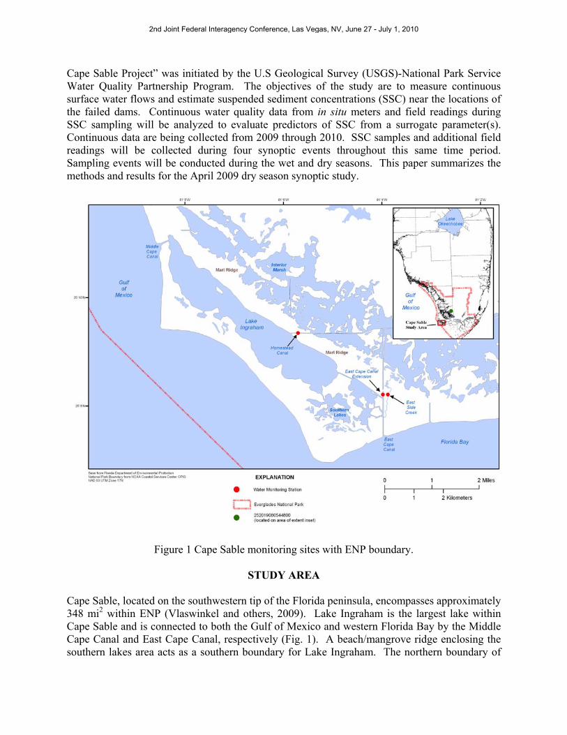
The Cape Sable peninsula is located within Everglades National Park (ENP) on the southwestern tip of the Florida peninsula (Fig. 1). Lake Ingraham, the largest lake within Cape Sable, has been connected to the Gulf of Mexico and western edge of Florida Bay as a result of canal construction that was completed in the early 1920’s. Prior to construction of the canals, Lake Ingraham had minimal connections to the Gulf of Mexico and Florida Bay (Wanless and others, 2005). Some of the canals were cut through a natural marl ridge to drain the interior marsh to promote agricultural and residential development in the area. The connections to the Gulf of Mexico and Florida Bay through the Middle Cape and East Cape Canals, respectively, allowed for continuous tidal flows to Lake Ingraham and the interior marsh, which increased the salinity in these water bodies. The tidal flows also increased sedimentation in Lake Ingraham from the interior marsh and Florida Bay. These connections have resulted in increased saline intrusion in the marsh that damaged vegetation and, as a result, increased erosion (Vlaswinkel and others, 2009). To protect the interior marsh from tidal flows and saline intrusion, ENP installed earthen dams in the 1950’s and 1960’s (ENP, 2009). After the earthen dams failed in the early 1990’s, sheet pile dams were installed. By the late 1990’s, the sheet pile dams had failed resulting in continued saline intrusion into the interior marsh and erosion of sediments. In 2009, ENP received funding from the American Reinvestment and Recovery Act to restore the failed dams. Construction for the Cape Sable Canals Dam Restoration Project is scheduled to begin in October 2010. In order to gather baseline data prior to restoration of the dams on East Cape Canal Extension and the Homestead Canal, a study entitled “The Sediment Transport and Saline Intrusion on

2nd Joint Federal Interagency Conference, Las Vegas, NV, June 27 - July 1, 2010

Cape Sable Project” was initiated by the U.S Geological Survey (USGS)-National Park Service Water Quality Partnership Program. The objectives of the study are to measure continuous surface water flows and estimate suspended sediment concentrations (SSC) near the locations of the failed dams. Continuous water quality data from in situ meters and field readings during SSC sampling will be analyzed to evaluate predictors of SSC from a surrogate parameter(s). Continuous data are being collected from 2009 through 2010. SSC samples and additional field readings will be collected during four synoptic events throughout this same time period. Sampling events will be conducted during the wet and dry seasons. This paper summarizes the methods and results for the April 2009 dry season synoptic study.

Figure 1 Cape Sable monitoring sites with ENP boundary.

STUDY AREA

Cape Sable, located on the southwestern tip of the Florida peninsula, encompasses approximately 348 mi2 within ENP (Vlaswinkel and others, 2009). Lake Ingraham is the largest lake within Cape Sable and is connected to both the Gulf of Mexico and western Florida Bay by the Middle Cape Canal and East Cape Canal, respectively (Fig. 1). A beach/mangrove ridge enclosing the southern lakes area acts as a southern boundary for Lake Ingraham. The northern boundary of


Lake Ingraham is composed of a storm deposit known as the marl ridge, which separated Lake Ingraham from the interior marsh before channelization. The marl ridge has been breached by a series of smaller man-made canals and natural estuarine creeks, and high tides that periodically overtop the ridge. Cape Sable is dependent on seasonal rainfall to mitigate local salinity conditions. The Everglades experiences distinct wet (May to October) and dry (November to April) seasons. A USGS precipitation rain gage at Upstream North River (ID 252019080544800) measured 56.2 inches of rain in 2009 with approximately 83 % of the rainfall occurring in the wet season. The area is highly susceptible to damage from hurricanes. In the past century, landscape changes in Cape Sable have been linked to the following four major storms: 1926 (Great Miami Hurricane), 1935 (Labor Day Hurricane), 1960 (Hurricane Donna), and 1992 (Hurricane Andrew) (Wanless and Vlaswinkel, 2005).

METHODS

Station Instrumentation Three real-time surface water monitoring stations were installed in December 2008. One station was installed in the East Cape Canal Extension (N25°08’13”, W 81°03’59”) and another in the Homestead Canal (N25°09’21”, W 81°05’42”) downstream from the dams that have failed (Fig. 1). These two sites were selected to provide data for initial construction permits and to evaluate the current conditions prior to restoration of the dams. A third station was installed in East Side Creek (N25°08’13”, W 81°03’53) as a reference station to evaluate the effects of the Cape Sable Canals Dam Restoration Project.

Each station was instrumented to collect continuous water level, water velocity, salinity, temperature, and turbidity data every 15 minutes. An acoustic Doppler velocity meter (ADVM) was mounted off of the station platform near the channel bank to measure the water velocity of a portion of the canal as an index velocity and the water level. Water quality parameters were measured by a water quality sonde mounted at a fixed location in the cross section. The datum of the gage was determined using Global Position Systems (GPS) technology operating in static GPS mode (C. Lindstedt, Mactec Inc., written commun., 2009). Water level data are referenced to the North American Vertical Datum of 1988.

Discharge Computation he index velocity method was used to compute continuous discharge from a relation developed between the index velocities, measured by the ADVM, and the mean channel velocities. The mean channel velocities were determined from discharges measured over a range of tidal flows and water levels. Simple linear regression was used to develop the relation between the index velocity and the mean channel velocity. The index velocity method is discussed in more detail in Hittle and others (2001), Morlock and others (2002), and Ruhl and others (2005).

Discharge measurements were collected using an acoustic Doppler current profiler (ADCP). The collection and processing of discharge measurements using ADCPs is discussed in more detail in Oberg and others (2005) and Mueller and others (2009). Field water levels were verified by performing down-to-water measurements from a fixed point of known elevation. A relation between water level and the standard cross section was developed to compute the cross sectional


area for continuous records of discharge. The processing of continuous water level data is discussed in more detail in Sauer (2002).

Continuous Water Quality Data and Sampling Continuous salinity, temperature, and turbidity data were collected at a fixed location in the cross section. Water quality sondes were routinely serviced to maintain data quality and correct for fouling and electric drift when applicable. Field data were collected, processed and published following guidelines by Wagner and others (2006). In addition, cross sectional profiles of water temperature, salinity and turbidity were collected at each station during the synoptic to determine if the in situ monitor mounted at a fixed location was representative of the entire cross section.

One goal of the synoptic was to collect a large number of suspended sediment samples to develop the relation between in situ turbidity and SSC at each station. Automatic samplers were deployed at each monitoring station during the synoptic to collect SSC samples near the in situ turbidity sensors over roughly two tidal cycles. The automatic samplers were programmed to collect approximately 900 mL samples every 2 hours. A few cross sectional SSC samples were collected during the synoptic using a modified vertical sampling approach (MVS) to determine if the SSC collected from the automatic sampler was representative of the cross section (Wilde and others, 2008). The MVS was taken from five equally spaced locations across the stream perpendicular to flow. At each sampling location either a wading rod or weighted bottle sampler was used depending on the ambient flow conditions. During low flow conditions, a wide mouth polyethylene bottle was attached to a wading rod using a DH-81A adaptor, plastic cap, and 5/16 inch nozzle. During higher flow conditions a narrow mouth polyethylene bottle was inserted into a weighted bottle sampler using a 3/16 inch nozzle. The sample bottle was lowered to the desired depth and raised back to the surface at a relatively constant transit rate, which allowed the sampling bottle to collect the sample.

Analysis Methods All suspended sediment samples were shipped to the USGS Kentucky Water Science Center Sediment Laboratory for processing and analysis. The laboratory employed methods discussed by Guy (1969) for the processing of suspended sediment concentrations and sand/fine separation. All suspended sediment samples were processed using the filtration method because concentrations were less than 10,000 mg/L and were not dominated by sand or clay (Shreve and others, 2005). Analysis of sand/fine separation was performed on selected samples.

RESULTS The following section summarizes the continuous and discrete data collected on April 27-30, 2009. Continuously measured data include water level, discharge, turbidity, and salinity. A total of 156 discharge measurements and 149 suspended sediment samples were collected for the development of the water velocity and surrogate (turbidity) relations (Table 1). The index velocity rating and turbidity surrogate model from East Cape Canal Extension are presented.


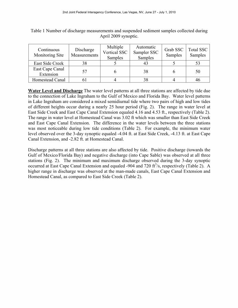
Table 1 Number of discharge measurements and suspended sediment samples collected during April 2009 synoptic.

Continuous Monitoring Site

Discharge Measurements

Multiple Vertical SSC

Samples

Automatic Sampler SSC

Samples

Grab SSC Samples

Total SSC Samples

East Side Creek 38 5 43 5 53 East Cape Canal

Extension 57 6 38 6 50

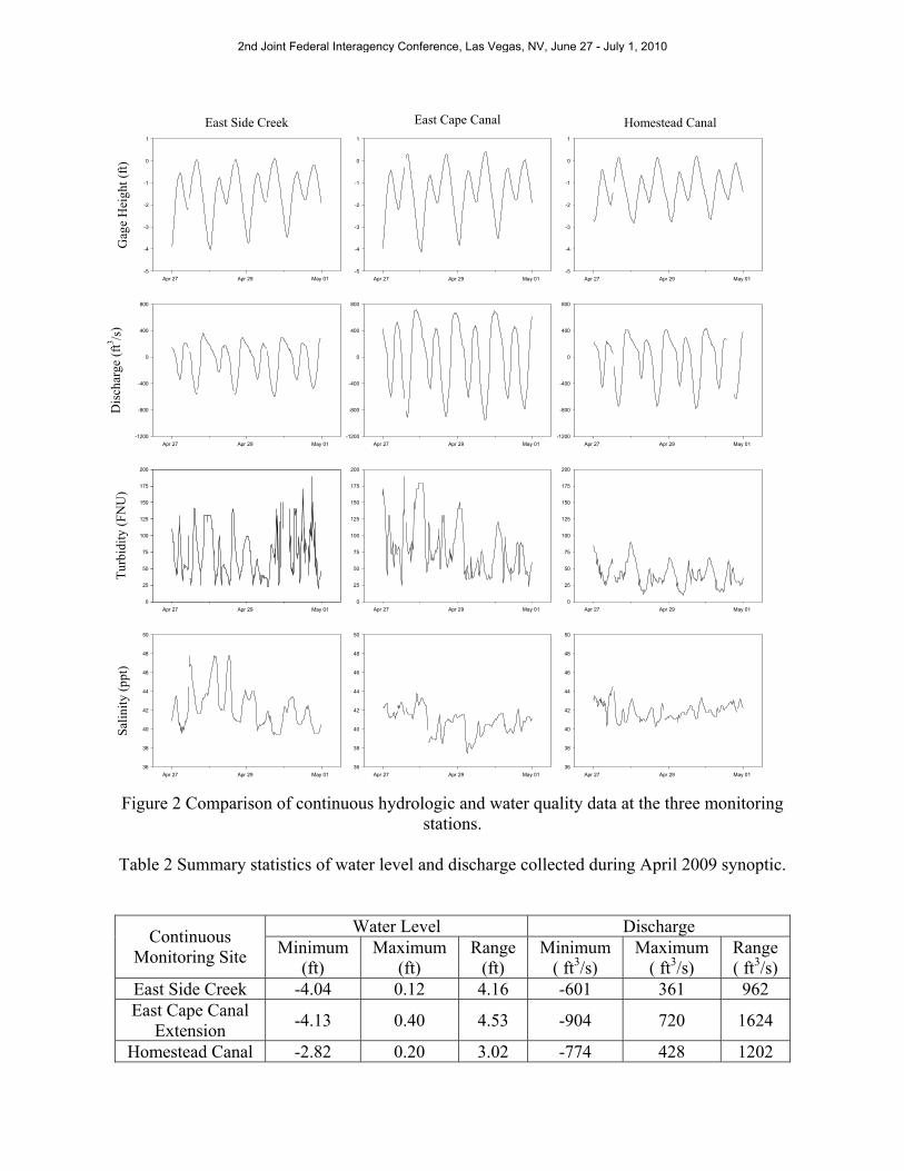
Homestead Canal 61 4 38 4 46 Water Level and Discharge The water level patterns at all three stations are affected by tide due to the connection of Lake Ingraham to the Gulf of Mexico and Florida Bay. Water level patterns in Lake Ingraham are considered a mixed semidiurnal tide where two pairs of high and low tides of different heights occur during a nearly 25 hour period (Fig. 2). The range in water level at East Side Creek and East Cape Canal Extension equaled 4.16 and 4.53 ft., respectively (Table 2). The range in water level at Homestead Canal was 3.02 ft which was smaller than East Side Creek and East Cape Canal Extension. The difference in the water levels between the three stations was most noticeable during low tide conditions (Table 2). For example, the minimum water level observed over the 3-day synoptic equaled -4.04 ft. at East Side Creek, -4.13 ft. at East Cape Canal Extension, and -2.82 ft. at Homestead Canal. Discharge patterns at all three stations are also affected by tide. Positive discharge (towards the Gulf of Mexico/Florida Bay) and negative discharge (into Cape Sable) was observed at all three stations (Fig. 2). The minimum and maximum discharge observed during the 3-day synoptic occurred at East Cape Canal Extension and equaled -904 and 720 ft3/s, respectively (Table 2). A higher range in discharge was observed at the man-made canals, East Cape Canal Extension and Homestead Canal, as compared to East Side Creek (Table 2).


East Side Creek

Apr 27 Apr 29 May 01

Gag

e H

eigh

t (ft

)

-5

-4

-3

-2

-1

0

1


Dis

char

ge (

ft3 /s

)

-1200

-800

-400

0

400

800


Tur

bidi

ty (

FN

U)

0

25

50

75

100

125

150

175

200


Sal

init

y (p

pt)

36

38

40

42

44

46

48

50

East Cape Canal


-5

-4

-3

-2

-1

0

1


-1200

-800

-400

0

400

800


0

25

50

75

100

125

150

175

200


36

38

40

42

44

46

48

50

Homestead Canal


-5

-4

-3

-2

-1

0

1


-1200

-800

-400

0

400

800


0

25

50

75

100

125

150

175

200


36

38

40

42

44

46

48

50

Figure 2 Comparison of continuous hydrologic and water quality data at the three monitoring

stations.

Table 2 Summary statistics of water level and discharge collected during April 2009 synoptic.

Water Level Discharge Continuous

Monitoring Site Minimum (ft)

Maximum (ft)

Range (ft)

Minimum ( ft3/s)

Maximum ( ft3/s)

Range ( ft3/s)

East Side Creek -4.04 0.12 4.16 -601 361 962 East Cape Canal

Extension -4.13 0.40 4.53 -904 720 1624

Homestead Canal -2.82 0.20 3.02 -774 428 1202


Turbidity and Salinity The range of in situ turbidity at East Side Creek, East Cape Canal and Homestead Canal equaled 170, and 167, and 81 Formazin Nephelometric Units (FNU), respectively (Table 3). The range of in situ turbidity at Homestead Canal was roughly half of the observed range at East Side Creek and East Cape Canal Extension. The continuous in situ turbidity values at East Side Creek increased on day 3 of the synoptic but the increase in turbidity was not observed at East Cape Canal Extension or Homestead Canal (Fig. 2). The majority of the outliers identified at East Side Creek during the development of the turbidity surrogate model occurred on April 30, 2009, which coincided with the increase in the in situ turbidity record. Erratic in situ turbidity data were observed at East Side Creek but not at East Cape Canal Extension and Homestead Canal. No independent measurements of turbidity were recorded on April 30th to confirm the accuracy of the in situ turbidity record at East Side Creek. The continuous in situ salinity was greater than 35 ppt at all three sites during the 3-day synoptic (Fig. 2). The median salinity values at East Side Creek, East Cape Canal Extension, and Homestead Canal equaled 41.8, 40.9, and 41.8 ppt, respectively (Table 3).

Table 3 Summary statistics of turbidity and salinity collected during the April 2009 synoptic.

Turbidity Salinity Continuous

Monitoring Site Minimum (FNU)

Maximum (FNU)

Median (FNU)

Minimum (ppt)

Maximum (ppt)

Median (ppt)

East Side Creek 20 190 60 39.5 47.8 41.8 East Cape Canal

Extension 23 190 74 37.4 43.8 40.9

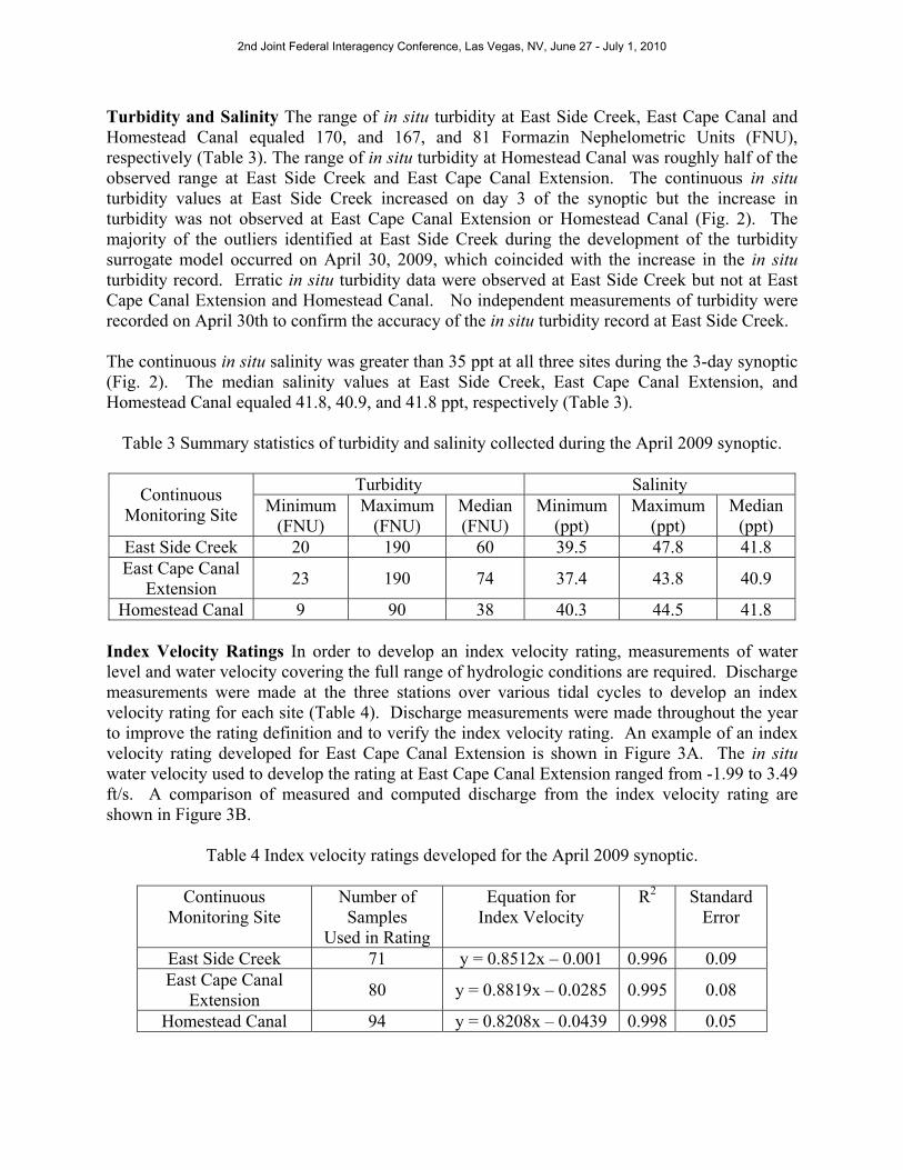
Homestead Canal 9 90 38 40.3 44.5 41.8 Index Velocity Ratings In order to develop an index velocity rating, measurements of water level and water velocity covering the full range of hydrologic conditions are required. Discharge measurements were made at the three stations over various tidal cycles to develop an index velocity rating for each site (Table 4). Discharge measurements were made throughout the year to improve the rating definition and to verify the index velocity rating. An example of an index velocity rating developed for East Cape Canal Extension is shown in Figure 3A. The in situ water velocity used to develop the rating at East Cape Canal Extension ranged from -1.99 to 3.49 ft/s. A comparison of measured and computed discharge from the index velocity rating are shown in Figure 3B.

Table 4 Index velocity ratings developed for the April 2009 synoptic.


Number of Samples

Used in Rating

Equation for Index Velocity

R2 Standard Error

East Side Creek 71 y = 0.8512x – 0.001 0.996 0.09 East Cape Canal

Extension 80 y = 0.8819x – 0.0285 0.995 0.08

Homestead Canal 94 y = 0.8208x – 0.0439 0.998 0.05


Apr 27 Apr 28 Apr 29 Apr 30

Dis

char

ge (

ft3 /s

)

-1200

-1000

-800

-600

-400

-200

0

200

400

600

800

1000

Computed Discharge

ADCP Measurements

Sontek Velocity (ft/s)

-2 0 2 4

Mea

sure

d V

eloc

ity

(ft/

s)

-3

-2

-1

0

1

2

3

4

Index Velocity Rating Points

y = 0.8819x - 0.0285 R2

= 0.9948

A B

Figure 3 (A) Index velocity rating developed for East Cape Canal Extension, (B) A comparison

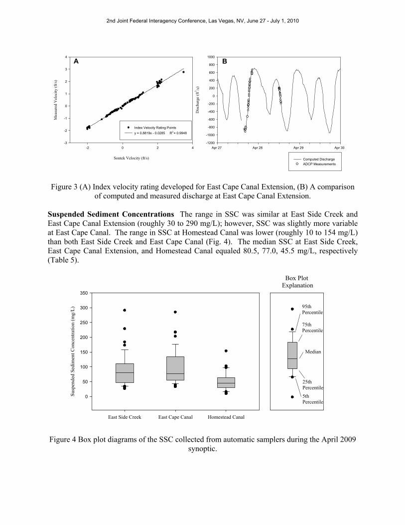
of computed and measured discharge at East Cape Canal Extension. Suspended Sediment Concentrations The range in SSC was similar at East Side Creek and East Cape Canal Extension (roughly 30 to 290 mg/L); however, SSC was slightly more variable at East Cape Canal. The range in SSC at Homestead Canal was lower (roughly 10 to 154 mg/L) than both East Side Creek and East Cape Canal (Fig. 4). The median SSC at East Side Creek, East Cape Canal Extension, and Homestead Canal equaled 80.5, 77.0, 45.5 mg/L, respectively (Table 5).

East Side Creek East Cape Canal Homestead Canal

Sus

pend

ed S

edim

ent C

once

ntra

tion

(m

g/L

)

0

50

100

150

200

250

300

350

Box Plot Explanation

95thPercentile

75thPercentile

25thPercentile

5th Percentile

Median

Figure 4 Box plot diagrams of the SSC collected from automatic samplers during the April 2009 synoptic.


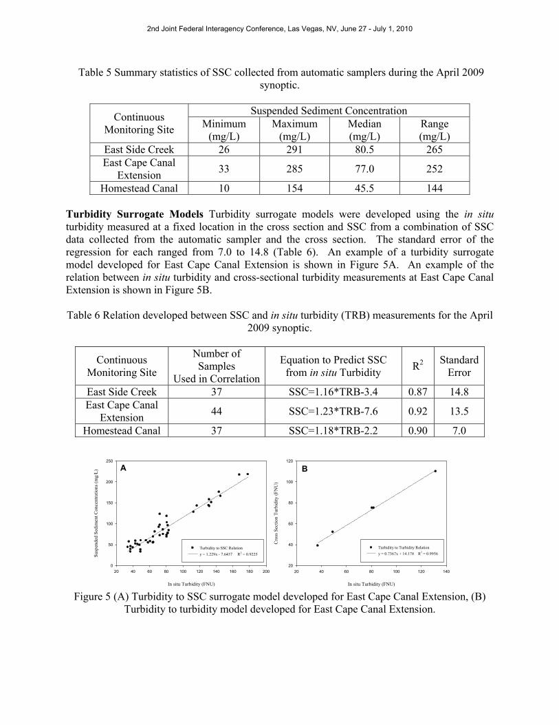
Table 5 Summary statistics of SSC collected from automatic samplers during the April 2009 synoptic.

Suspended Sediment Concentration

Continuous Monitoring Site Minimum

(mg/L) Maximum

(mg/L) Median (mg/L)

Range (mg/L)

East Side Creek 26 291 80.5 265 East Cape Canal

Extension 33 285 77.0 252

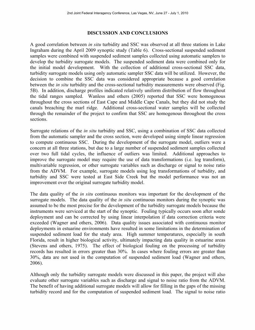
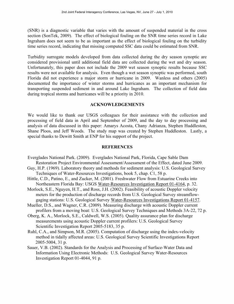
Homestead Canal 10 154 45.5 144 Turbidity Surrogate Models Turbidity surrogate models were developed using the in situ turbidity measured at a fixed location in the cross section and SSC from a combination of SSC data collected from the automatic sampler and the cross section. The standard error of the regression for each ranged from 7.0 to 14.8 (Table 6). An example of a turbidity surrogate model developed for East Cape Canal Extension is shown in Figure 5A. An example of the relation between in situ turbidity and cross-sectional turbidity measurements at East Cape Canal Extension is shown in Figure 5B. Table 6 Relation developed between SSC and in situ turbidity (TRB) measurements for the April

2009 synoptic.


Number of Samples

Used in Correlation

Equation to Predict SSC from in situ Turbidity

R2 Standard

Error

East Side Creek 37 SSC=1.16*TRB-3.4 0.87 14.8 East Cape Canal

Extension 44 SSC=1.23*TRB-7.6 0.92 13.5

Homestead Canal 37 SSC=1.18*TRB-2.2 0.90 7.0

In situ Turbidity (FNU)

20 40 60 80 100 120 140 160 180 200

Sus

pend

ed S

edim

ent C

once

ntra

tions

(m

g/L

)

0

50

100

150

200

250

Turbidity to SSC Relation

y = 1.229x - 7.6437 R2 = 0.9225

In situ Turbidity (FNU)

20 40 60 80 100 120 140

Cro

ss S

ectio

n T

urbi

dity

(F

NU

)

20

40

60

80

100

120

Turbidity to Turbidity Relation

y = 0.7367x + 14.178 R2 = 0.9956

A B

Figure 5 (A) Turbidity to SSC surrogate model developed for East Cape Canal Extension, (B)

Turbidity to turbidity model developed for East Cape Canal Extension.


DISCUSSION AND CONCLUSIONS

A good correlation between in situ turbidity and SSC was observed at all three stations in Lake Ingraham during the April 2009 synoptic study (Table 6). Cross-sectional suspended sediment samples were combined with suspended sediment samples collected using automatic samplers to develop the turbidity surrogate models. The suspended sediment data were combined only for the initial model development. With the collection of additional cross-sectional SSC data, turbidity surrogate models using only automatic sampler SSC data will be utilized. However, the decision to combine the SSC data was considered appropriate because a good correlation between the in situ turbidity and the cross-sectional turbidity measurements were observed (Fig. 5B). In addition, discharge profiles indicated relatively uniform distribution of flow throughout the tidal ranges sampled. Wanless and others (2005) reported that SSC were homogenous throughout the cross sections of East Cape and Middle Cape Canals, but they did not study the canals breaching the marl ridge. Additional cross-sectional water samples will be collected through the remainder of the project to confirm that SSC are homogenous throughout the cross sections. Surrogate relations of the in situ turbidity and SSC, using a combination of SSC data collected from the automatic sampler and the cross section, were developed using simple linear regression to compute continuous SSC. During the development of the surrogate model, outliers were a concern at all three stations, but due to a large number of suspended sediment samples collected over two full tidal cycles, the influence of outliers was limited. Additional approaches to improve the surrogate model may require the use of data transformations (i.e. log transform), multivariable regression, or other surrogate variables such as discharge or signal to noise ratio from the ADVM. For example, surrogate models using log transformations of turbidity, and turbidity and SSC were tested at East Side Creek but the model performance was not an improvement over the original surrogate turbidity model.

The data quality of the in situ continuous monitors was important for the development of the surrogate models. The data quality of the in situ continuous monitors during the synoptic was assumed to be the most precise for the development of the turbidity surrogate models because the instruments were serviced at the start of the synoptic. Fouling typically occurs soon after sonde deployment and can be corrected by using linear interpolation if data correction criteria were exceeded (Wagner and others, 2006). Data quality issues associated with continuous monitor deployments in estuarine environments have resulted in some limitations in the determination of suspended sediment load for the study area. High summer temperatures, especially in south Florida, result in higher biological activity, ultimately impacting data quality in estuarine areas (Stevens and others, 1975). The effect of biological fouling on the processing of turbidity records has resulted in errors greater than 30%. In cases where fouling errors are greater than 30%, data are not used in the computation of suspended sediment load (Wagner and others, 2006).

Although only the turbidity surrogate models were discussed in this paper, the project will also evaluate other surrogate variables such as discharge and signal to noise ratio from the ADVM. The benefit of having additional surrogate models will allow for filling in the gaps of the missing turbidity record and for the computation of suspended sediment load. The signal to noise ratio


(SNR) is a diagnostic variable that varies with the amount of suspended material in the cross section (SonTek, 2009). The effect of biological fouling on the SNR time series record in Lake Ingraham does not seem to be as important as the effect of biological fouling on the turbidity time series record, indicating that missing computed SSC data could be estimated from SNR. Turbidity surrogate models developed from data collected during the dry season synoptic are considered provisional until additional field data are collected during the wet and dry season. Unfortunately, this paper does not include the 2009 wet season synoptic results because SSC results were not available for analysis. Even though a wet season synoptic was performed, south Florida did not experience a major storm or hurricane in 2009. Wanless and others (2005) documented the importance of winter storms and hurricanes as an important mechanism for transporting suspended sediment in and around Lake Ingraham. The collection of field data during tropical storms and hurricanes will be a priority in 2010.

ACKNOWLEDGEMENTS

We would like to thank our USGS colleagues for their assistance with the collection and processing of field data in April and September of 2009, and the day to day processing and analysis of data discussed in this paper: Amarys Acosta, Chany Adrianza, Stephen Huddleston, Shane Ploos, and Jeff Woods. The study map was created by Stephen Huddleston. Lastly, a special thanks to Dewitt Smith at ENP for his support of the project.

REFERENCES

Everglades National Park. (2009). Everglades National Park, Florida, Cape Sable Dam

Restoration Project Environmental Assessment/Assessment of the Effect, dated June 2009. Guy, H.P. (1969). Laboratory theory and methods for sediment analysis: U.S. Geological Survey

Techniques of Water-Resources Investigations, book 5, chap. C1, 58 p. Hittle, C.D., Patino, E., and Zucker, M. (2001). Freshwater Flow from Estuarine Creeks into

Northeastern Florida Bay: USGS Water-Resources Investigation Report 01-4164, p. 32. Morlock, S.E., Nguyen, H.T., and Ross, J.H. (2002). Feasibility of acoustic Doppler velocity

meters for the production of discharge records from U.S. Geological Survey streamflow-gaging stations: U.S. Geological Survey Water-Resources Investigations Report 01-4157.

Mueller, D.S., and Wagner, C.R. (2009). Measuring discharge with acoustic Doppler current profilers from a moving boat: U.S. Geological Survey Techniques and Methods 3A-22, 72 p.

Oberg, K. A., Morlock, S.E., Caldwell, W.S. (2005). Quality assurance plan for discharge measurements using acoustic Doppler current profilers: U.S. Geological Survey Scientific Investigation Report 2005-5183, 35 p.

Ruhl, C.A., and Simpson, M.R. (2005). Computation of discharge using the index-velocity method in tidally affected areas: U.S. Geological Survey Scientific Investigations Report 2005-5004, 31 p.

Sauer, V.B. (2002). Standards for the Analysis and Processing of Surface-Water Data and Information Using Electronic Methods: U.S. Geological Survey Water-Resources Investigation Report 01-4044, 91 p.


Shreve, E.A., and Downs, A.C. (2005). Quality-Assurance Plan for the Analysis of Fluvial Sediment by the U.S. Geological Survey Kentucky Water Science Center Sediment Laboratory: U.S. Geological Survey Open-File Report 2005-1230, 28 p.

SonTek. (2009). SonTek Argonaut-SL System Manual: San Diego, Calif., 330 p. Stevens, H.H., Ficke, J.F., and Smoot, G.F. (1975). Water temperature - Influential factors, field

measurement, and data presentation: U.S. Geological Survey Techniques of Water-Resources Investigations, book 1, chap. D1, 65 p.

Vlaswinkel, B.M. and Wanless, H.R. (2009). Rapid recycling and deposition of organic-rich carbonates within the coastal complex of southwest Florida, In: Perspectives in Carbonate Geology: IAS Special Publication no. 41.

Wagner, R.J., Boulger, R.W., Jr., Oblinger, C.J., and Smith, B.A. (2006). Guidelines and standard procedures for continuous water-quality monitors—Station operation, record computation, and data reporting: U.S. Geological Survey Techniques and Methods 1–D3, 51 p. at http://pubs.water.usgs.gov/tm1d3.

Wanless, H.R and Vlaswinkel, B.M. (2005). Coastal landscape and Channel Evolution Affecting Critical Habitats at Cape Sable, Everglades National Park.

Wilde, F.D., ed. (2008). Field measurements: U.S. Geological Survey Techniques of Water- Resources Investigations, book 9, chap. A6, at http://pubs.water.usgs.gov/twri9A6/.


Documents

SEDIMENT TRANSPORT ON CAPE SABLE, EVERGLADES NATIONAL PARK