Embed Size (px)
Citation preview
MAE 5420 - Compressible Fluid Flow 1
Section 3: Lecture 2 ���Alternative Forms of the One-Dimensional
Energy Equation
Anderson: Chapter 3 pp. 71-86
MAE 5420 - Compressible Fluid Flow 2
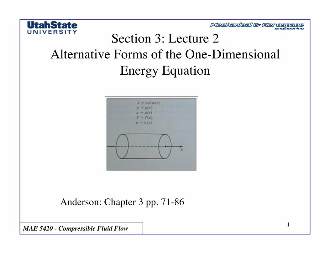
Review: 1-D, Steady, Flow: Collected Equations
• Continuity
• Momentum
• Energy
→ ρiVi = ρeVe
→ pi + ρiVi2 = pe + ρeVe
2
→ q•+ hi +
Vi2
2= he +
Ve2
2
MAE 5420 - Compressible Fluid Flow 3
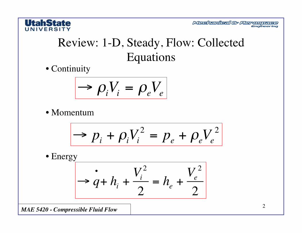
Review:���Effect of Mach Number on Flow Properties
Mach number is a measure of the ratio of the fluid Kinetic energy to the fluid internal energy (direct motion To random thermal motion of gas molecules)
V 2
2e
=V 2
2cvT
=V 2
2Rgγ −1⎛
⎝⎜⎞
⎠⎟T=
γγ
V 2
2Rgγ −1⎛
⎝⎜⎞
⎠⎟T=γ γ −1( )2
V 2
γ RgT=γ γ −1( )2
M 2
MAE 5420 - Compressible Fluid Flow 4
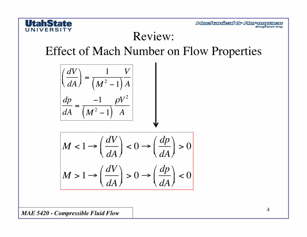
Review:���Effect of Mach Number on Flow Properties
dVdA
⎛⎝⎜
⎞⎠⎟=
1M 2 −1( )
VA
dpdA
=−1
M 2 −1( )ρV 2
A
M < 1→ dVdA
⎛⎝⎜
⎞⎠⎟< 0→ dp
dA⎛⎝⎜
⎞⎠⎟> 0
M > 1→ dVdA
⎛⎝⎜
⎞⎠⎟> 0→ dp
dA⎛⎝⎜
⎞⎠⎟< 0

MAE 5420 - Compressible Fluid Flow 5
Review:���Fundamental Properties of Supersonic���
and Supersonic Flow
MAE 5420 - Compressible Fluid Flow 6
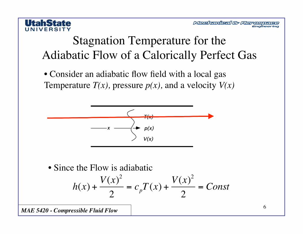
Stagnation Temperature for the���Adiabatic Flow of a Calorically Perfect Gas • Consider an adiabatic flow field with a local gas Temperature T(x), pressure p(x), and a velocity V(x)
x
T(x)
V(x)
p(x)
• Since the Flow is adiabatic
h(x) + V (x)2
2= cpT (x) +
V (x)2
2= Const
MAE 5420 - Compressible Fluid Flow 7
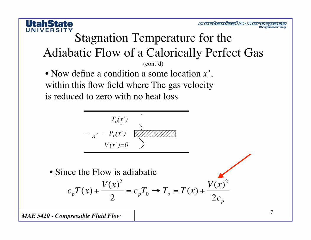
Stagnation Temperature for the���Adiabatic Flow of a Calorically Perfect Gas
(cont’d) • Now define a condition a some location x’, within this flow field where The gas velocity is reduced to zero with no heat loss
• Since the Flow is adiabatic
y
To(y)
V(y)=0
po(y)
cpT (x) +V (x)2
2= cpT0 → To = T (x) +
V (x)2
2cp
T0(x’)
P0(x’) V (x’)=0
x’

MAE 5420 - Compressible Fluid Flow 8
Stagnation Temperature for the���Adiabatic Flow of a Calorically Perfect Gas
(cont’d) • From Earlier Analysis
V 2
2cvT
=γ γ −1( )2
M 2 →
V 2
2γ cv=
V 2
2cpcvcv=V 2
2cp= T
γ −1( )2
M 2
• Therefore
To = T (x) + T (x)γ −1( )2
M (x)2Holds anywhere Within an adiabatic Flow field

MAE 5420 - Compressible Fluid Flow 9
Stagnation Temperature for the���Adiabatic Flow of a Calorically Perfect Gas (cont’d)
• In general for an adiabatic Flow Field the Stagnation Temperature is defined by the relationship
• Stagnation Temperature is Constant Throughout An adiabatic Flow Field
• T0 is also sometimes referred to at Total Temperature
• T is sometimes referred to as Static Temperature
T0T= 1+
γ −1( )2
M 2
MAE 5420 - Compressible Fluid Flow 10
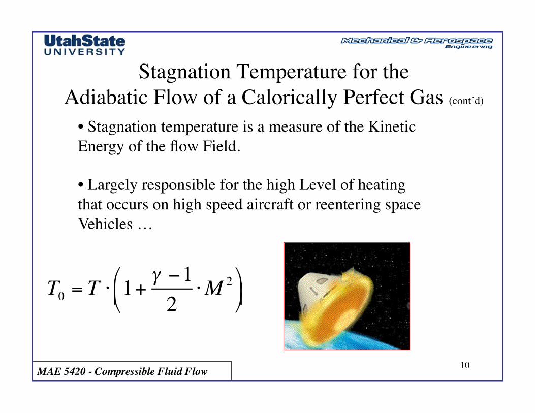
Stagnation Temperature for the���Adiabatic Flow of a Calorically Perfect Gas (cont’d)
• Stagnation temperature is a measure of the Kinetic Energy of the flow Field.
• Largely responsible for the high Level of heating that occurs on high speed aircraft or reentering space Vehicles …
T0 = T ⋅ 1+γ −12
⋅M 2⎛⎝⎜
⎞⎠⎟

MAE 5420 - Compressible Fluid Flow 11
Hypersonic Flow of a “Real Gas” ?
Let’s Revisit Hypersonic Flow
MAE 5420 - Compressible Fluid Flow 12
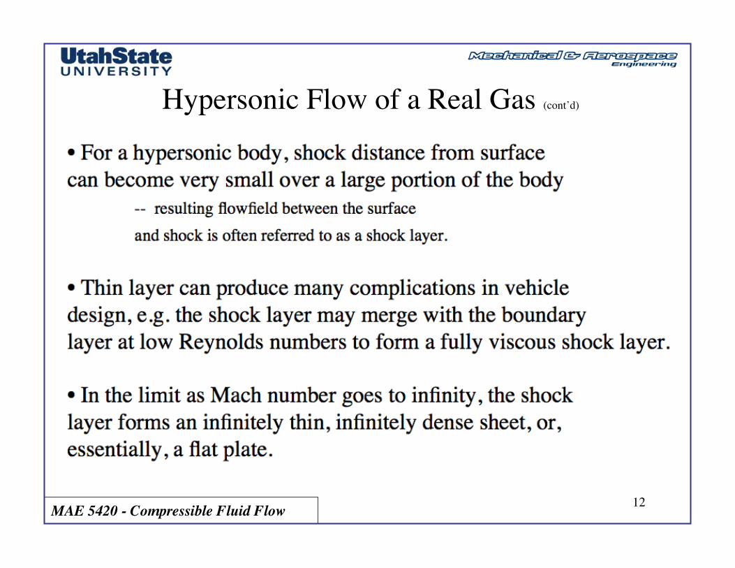
Hypersonic Flow of a Real Gas (cont’d)
MAE 5420 - Compressible Fluid Flow 13
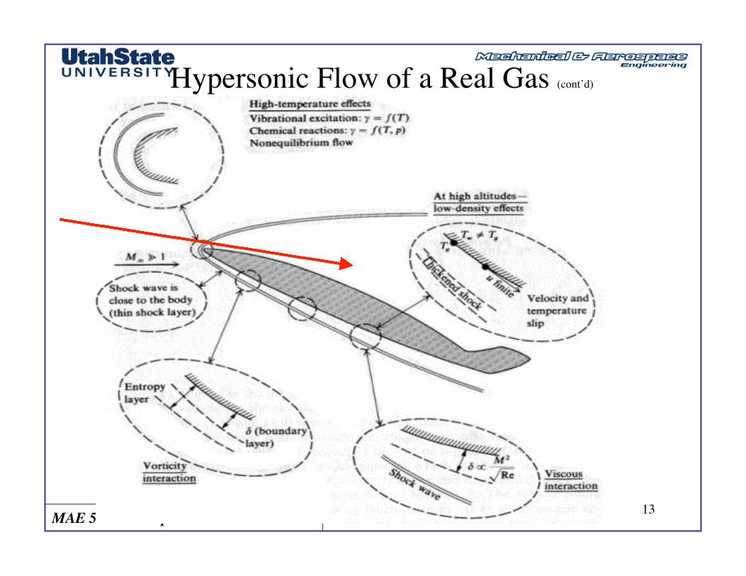
Hypersonic Flow of a Real Gas (cont’d)
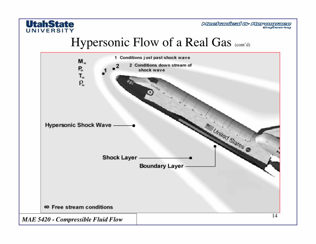
MAE 5420 - Compressible Fluid Flow 14
Hypersonic Flow of a Real Gas (cont’d) ���

MAE 5420 - Compressible Fluid Flow 15
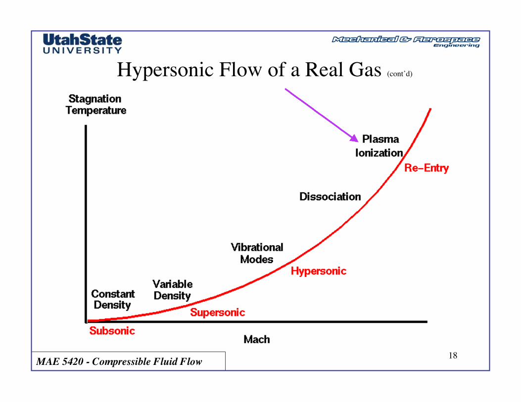
Hypersonic Flow of a Real Gas (cont’d) ���•Hypersonic vehicles dissipate so much kinetic energy and Produce such high temperatures due to shock wave that they cause chemical changes to occur in the fluid through which they fly.
• Gas chemistry effects are important factor in dissipation of heat on hypersonic vehicles

MAE 5420 - Compressible Fluid Flow 16
Hypersonic Flow of a Real Gas (cont’d) ���
cp =∂h∂T
→ cp ,cv ,γ{ }≠Const
MAE 5420 - Compressible Fluid Flow 17
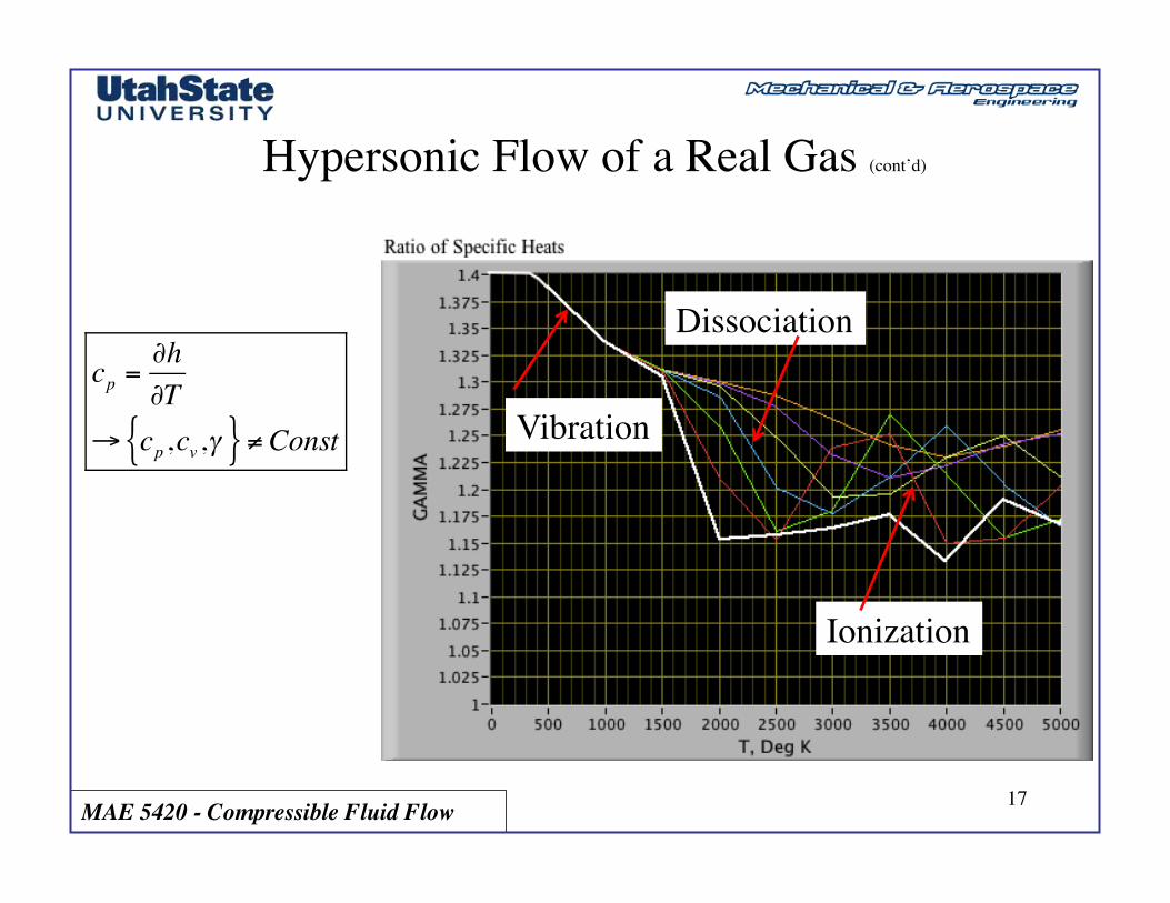
Hypersonic Flow of a Real Gas (cont’d) ���
cp =∂h∂T
→ cp ,cv ,γ{ }≠Const Vibration
Dissociation
Ionization
MAE 5420 - Compressible Fluid Flow 18
Hypersonic Flow of a Real Gas (cont’d) ���
MAE 5420 - Compressible Fluid Flow 19
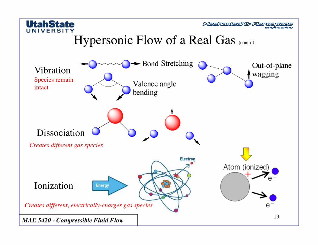
Hypersonic Flow of a Real Gas (cont’d) ���
Vibration Species remain intact
Dissociation
Ionization
Creates different gas species
Creates different, electrically-charges gas species
MAE 5420 - Compressible Fluid Flow 20
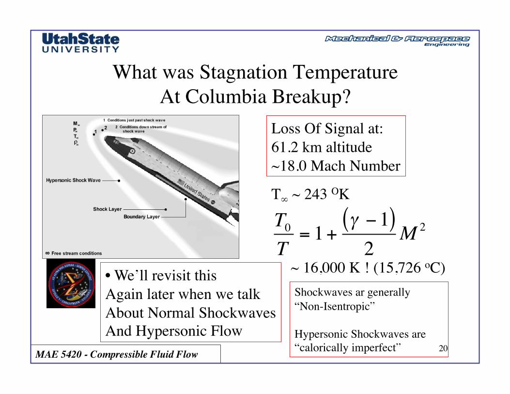
What was Stagnation Temperature���At Columbia Breakup?
Loss Of Signal at: 61.2 km altitude ~18.0 Mach Number
T∞ ~ 243 ΟK
T0T= 1+
γ −1( )2
M 2
• We’ll revisit this Again later when we talk About Normal Shockwaves And Hypersonic Flow
Shockwaves ar generally “Non-Isentropic”
Hypersonic Shockwaves are “calorically imperfect”
~ 16,000 K ! (15,726 oC)
MAE 5420 - Compressible Fluid Flow 21
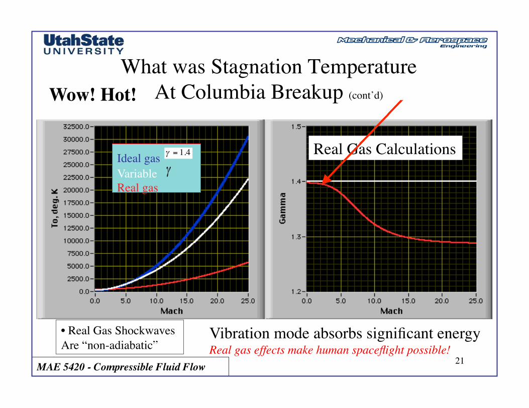
What was Stagnation Temperature���At Columbia Breakup (cont’d) Wow! Hot!
Ideal gas Variable Real gas
• Real Gas Shockwaves Are “non-adiabatic”
γγ = 1.4 Real Gas Calculations
Vibration mode absorbs significant energy Real gas effects make human spaceflight possible!
MAE 5420 - Compressible Fluid Flow 22
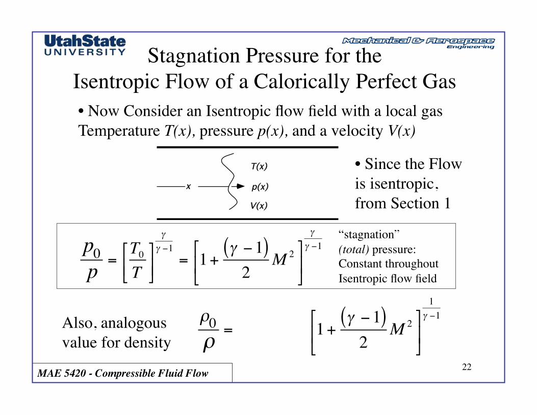
Stagnation Pressure for the���Isentropic Flow of a Calorically Perfect Gas • Now Consider an Isentropic flow field with a local gas Temperature T(x), pressure p(x), and a velocity V(x)
x
T(x)
V(x)
p(x)
• Since the Flow is isentropic, from Section 1
p0p =
T0T⎡
⎣⎢⎤
⎦⎥
γ
γ −1= 1+
γ −1( )2
M 2⎡
⎣⎢
⎤
⎦⎥
γ
γ −1“stagnation” (total) pressure: Constant throughout Isentropic flow field
ρ0ρ
=T0T⎡
⎣⎢⎤
⎦⎥
γ
γ −1= 1+
γ −1( )2
M 2⎡
⎣⎢
⎤
⎦⎥
1γ −1Also, analogous
value for density

MAE 5420 - Compressible Fluid Flow 23
Characteristic or “Sonic” Flow Parameters ���for Isentropic Flow Fields
x
T(x)
V(x)
p(x)
y
To(y)
V(y)=0
po(y)
• Stagnation properties Of a flow field result when Flow is isentropically Slowed from local velocity To zero
y
To(y)
V(y)=0
po(y)
T0(x’)
P0(x’) V (x’)=0
x’

MAE 5420 - Compressible Fluid Flow 24
Characteristic or “Sonic” Flow Parameters ���for Isentropic Flow Fields (cont’d)
x
T(x)
V(x)
p(x) • Define a new set of parameters where flow field is Either decelerated (supersonic) or accelerated (subsonic) From local velocity to sonic velocity -- { T*,P*,ρ* …}
yT*P*c*
x’
MAE 5420 - Compressible Fluid Flow 25
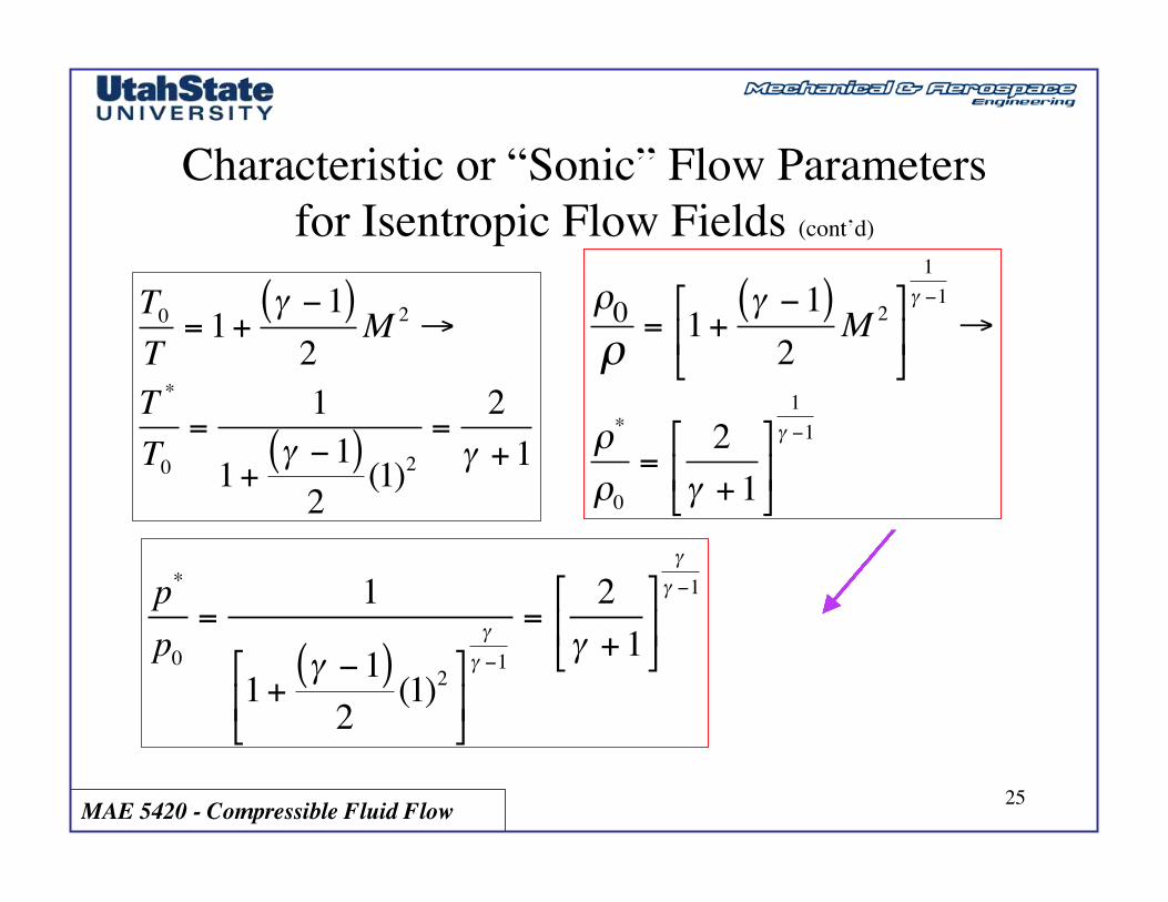
Characteristic or “Sonic” Flow Parameters ���for Isentropic Flow Fields (cont’d)
T0T= 1+
γ −1( )2
M 2 →
T *
T0=
1
1+γ −1( )2
(1)2=
2γ +1
p*
p0=
1
1+γ −1( )2
(1)2⎡
⎣⎢
⎤
⎦⎥
γ
γ −1
=2
γ +1⎡
⎣⎢
⎤
⎦⎥
γ
γ −1
ρ0ρ
= 1+γ −1( )2
M 2⎡
⎣⎢
⎤
⎦⎥
1γ −1
→
ρ*
ρ0=
2γ +1⎡
⎣⎢
⎤
⎦⎥
1γ −1
MAE 5420 - Compressible Fluid Flow 26
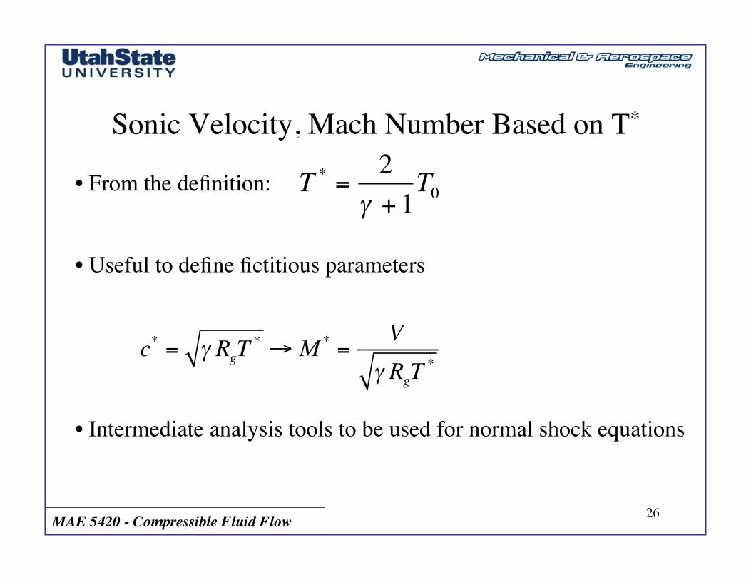
Sonic Velocity, Mach Number Based on T*
• From the definition:
• Useful to define fictitious parameters
• Intermediate analysis tools to be used for normal shock equations
T * =2
γ +1T0
c* = γ RgT* → M * =
Vγ RgT
*

MAE 5420 - Compressible Fluid Flow 27
Sonic Velocity, Mach Number Based on T*���(cont’d)
• From Energy equation for adiabatic flow
cpT +V 2
2= cpT
* +c*2
2→
γγ −1
RgT +V 2
2=
γγ −1
RgT* +
c*2
2→
c2
γ −1+V 2
2=
c*2
γ −1+c*2
2=
γ +12 γ −1( )
c*2

MAE 5420 - Compressible Fluid Flow 28
Sonic Velocity, Mach Number Based on T*���(concluded)
• Reorganizing terms
2c /V( )2
γ −1+1 = γ +1
γ −1( )c* /V( )2 →
2M 2 γ −1( )
=γ +1
M *2 γ −1( )−1→
1M 2 =
12γ +1M *2 −
γ −1( )2
→
M 2 =1
12γ +1M *2 −
γ −1( )2
=2M *2
γ +1− γ −1( )M *2
• M* = “characteristic Mach number”

MAE 5420 - Compressible Fluid Flow
Characteristic Mach Number (M*)
29
• One undesirable characteristic of the true Mach number is that it is not directly indicative of the local flow velocity.
—> Sonic velocity itself is also function of temperature.
• Consider two fluid particles that are proceeding within the first stage of a compressor and that of a turbine section with the same velocity.
—> Because the compressor particle is exposed to a much lower temperature than the turbine particle, the sonic speeds at these locations will be significantly different, and so will the Mach numbers.
• Sometimes it is advantageous to replace the Mach number with an alternative nondimensional-velocity ratio
—> the magnitude of M* is more directly indicative of the local velocity. ! M* approaches a constant value at high velocities

MAE 5420 - Compressible Fluid Flow 30
MAE 5420 - Compressible Fluid Flow
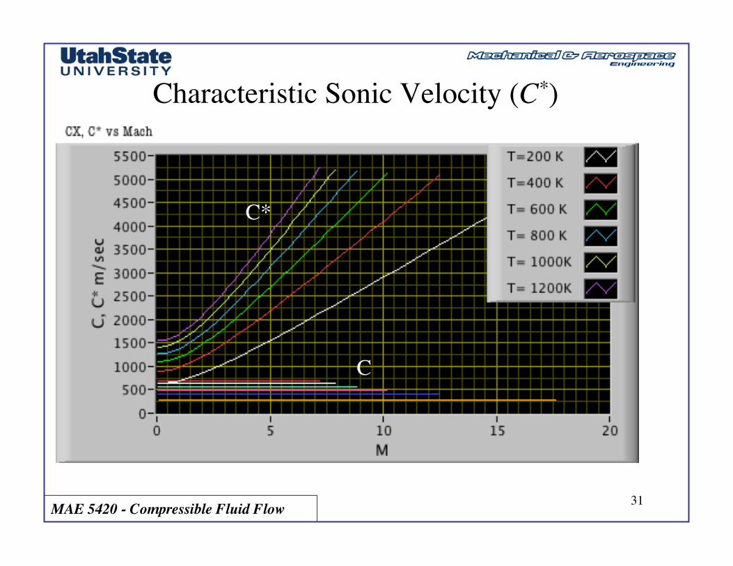
Characteristic Sonic Velocity (C*)
31
C*
C

MAE 5420 - Compressible Fluid Flow
Characteristic Sonic Velocity (C*)
32
C*
C
MAE 5420 - Compressible Fluid Flow 33
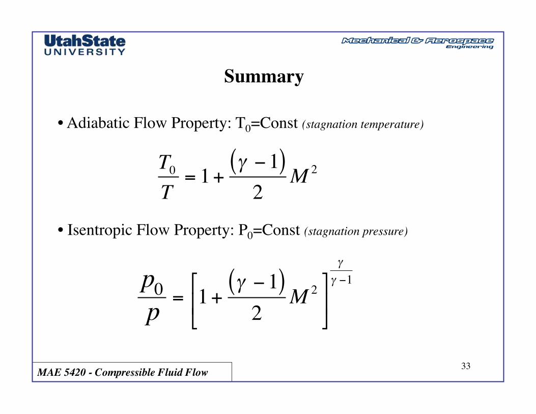
Summary
• Adiabatic Flow Property: T0=Const (stagnation temperature)
• Isentropic Flow Property: P0=Const (stagnation pressure)
T0T= 1+
γ −1( )2
M 2
p0p = 1+
γ −1( )2
M 2⎡
⎣⎢
⎤
⎦⎥
γ
γ −1
MAE 5420 - Compressible Fluid Flow
34
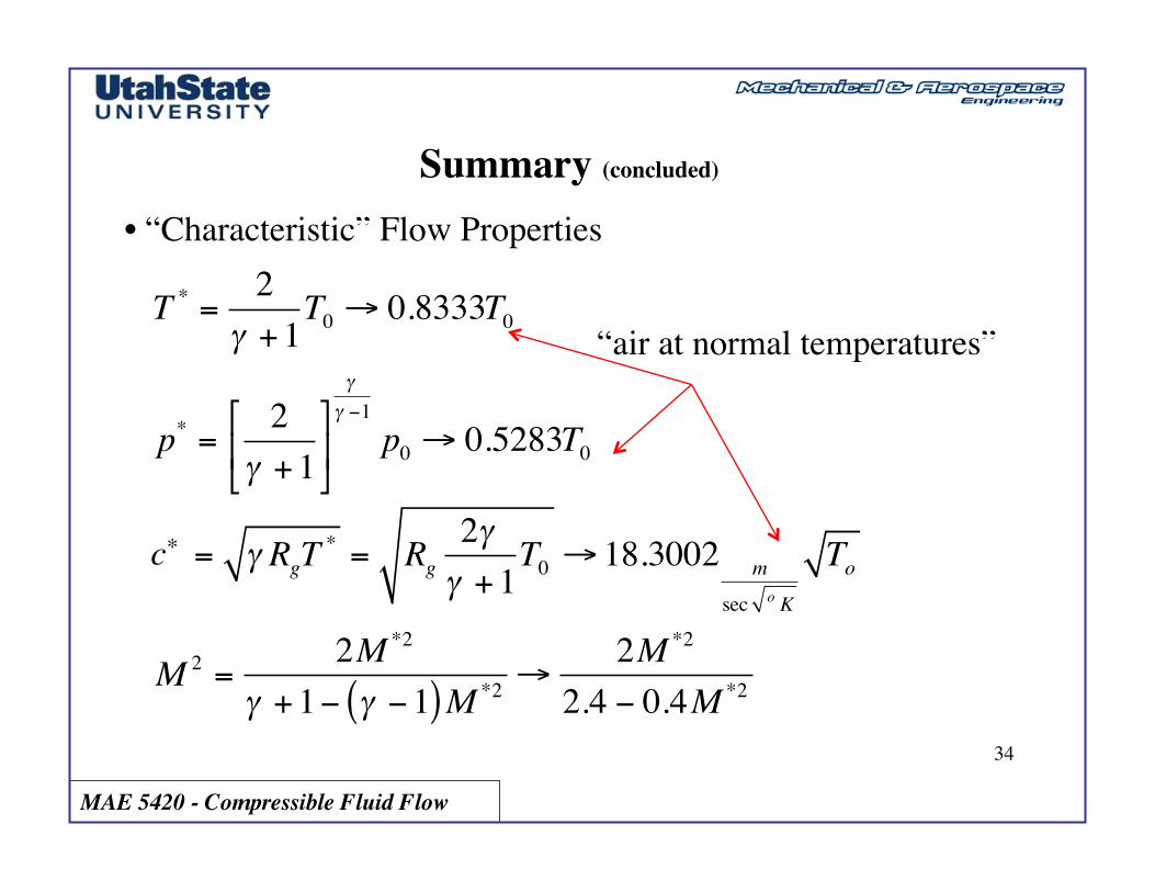
Summary (concluded) • “Characteristic” Flow Properties
T * =2
γ +1T0 → 0.8333T0
p* = 2γ +1⎡
⎣⎢
⎤
⎦⎥
γ
γ −1p0 → 0.5283T0
a* = γ RgT* = Rg
2γγ +1
T0 → 18.3002 m
sec o K
To
M 2 =2M *2
γ +1− γ −1( )M *2 →2M *2
2.4 − 0.4M *2
“air at normal temperatures”
c*

MAE 5420 - Compressible Fluid Flow 35
Revisit De Laval Nozzle
• What Pressure Ratio “Choked” De Laval’s Nozzles?
Assume VI ≈ 0
for Mt =1→ pt = p* pIpt( )
=γ +1
2⎛
⎝⎜
⎞
⎠⎟
γγ+1→ steam ≡
γ ≈ 1.286pIpt=1.824
MAE 5420 - Compressible Fluid Flow 36
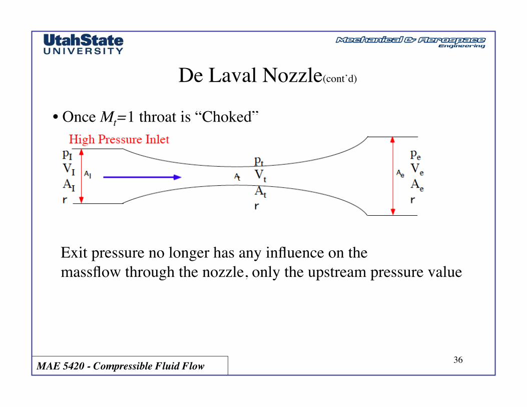
De Laval Nozzle(cont’d)
• Once Mt=1 throat is “Choked”
Exit pressure no longer has any influence on the massflow through the nozzle, only the upstream pressure value
MAE 5420 - Compressible Fluid Flow 37
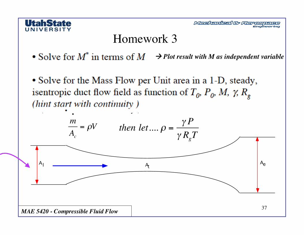
Homework 3
• Solve for M* in terms of M
• Solve for the Mass Flow per Unit area in a 1-D, steady, isentropic duct flow field as function of T0, P0, M, γ, Rg���(hint start with continuity )
m•
Ac= ρV
AeAI At
then let.... ρ = γ Pγ RgT
! Plot result with M as independent variable

MAE 5420 - Compressible Fluid Flow 38
Homework 3 (cont’d)
• Allowing that for isentropic flow .. Also show that for quasi 1-D flow
m•
A=
γRg
p0T0
M
1+γ −1( )2
M 2⎡
⎣⎢
⎤
⎦⎥
γ +12 γ −1( )
i.e. … Show that …. for Quasi 1-D isentropic flow
P0
T0T= 1+ γ −1
2M 2⎛
⎝⎜
⎞
⎠⎟
P0p= 1+ γ −1
2M 2⎛
⎝⎜
⎞
⎠⎟
γγ−1
→!mA= P0
2γγ −1( ) Rg ⋅T0( )
pP0
⎛
⎝⎜
⎞
⎠⎟
2γ
−pP0
⎛
⎝⎜
⎞
⎠⎟
γ+1γ
⎡
⎣
⎢⎢⎢
⎤
⎦
⎥⎥⎥
MAE 5420 - Compressible Fluid Flow 39
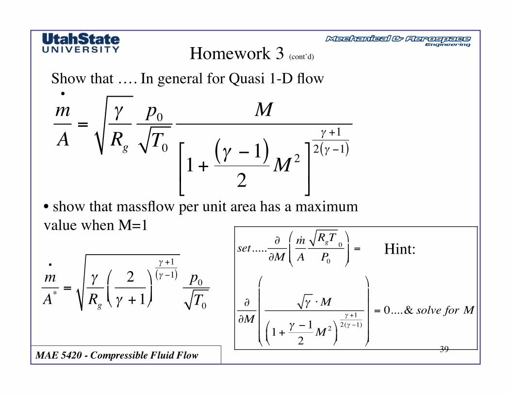
Homework 3 (cont’d)
• show that massflow per unit area has a maximum value when M=1
m•
A*=
γRg
2γ +1⎛
⎝⎜⎞
⎠⎟
γ +1γ −1( ) p0
T0
m•
A=
γRg
p0T0
M
1+γ −1( )2
M 2⎡
⎣⎢
⎤
⎦⎥
γ +12 γ −1( )
Show that …. In general for Quasi 1-D flow
Hint:
set..... ∂
∂M!mA
RgT 0
P0
⎛
⎝⎜⎜
⎞
⎠⎟⎟=
∂
∂Mγ ⋅M
1+ γ −12
M 2⎛⎝⎜
⎞⎠⎟
γ +12(γ −1)
⎛
⎝
⎜⎜⎜⎜⎜
⎞
⎠
⎟⎟⎟⎟⎟
= 0....& solve for M
MAE 5420 - Compressible Fluid Flow 40
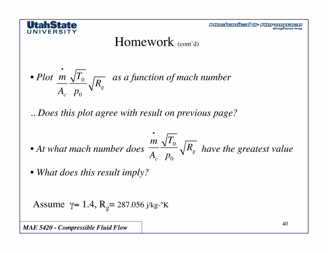
Homework (cont’d)
• Plot as a function of mach number
.. Does this plot agree with result on previous page?
• At what mach number does have the greatest value
• What does this result imply?
Assume γ= 1.4, Rg= 287.056 j/kg-°K
m•
Ac
T0p0
Rg
m•
Ac
T0p0
Rg