Embed Size (px)
Citation preview


UNIVERSITY OFILLINOIS LIBRARY
AT URBANA-CHAMPAIGNBOOKSTACKS

THE HECKMAN BINDERY, INC.
North Manchester, Indiana
JUST FONT SLOT TITLE
H CC 1
21 LTYWUuXING
19 PAPER
H CC N 8 1983-847 NO. 991-1
H CC
H CC
330B385<"CV">no. 991-1009cop. 2
<IMPRINT>U. of ILL.library"URBANA
DMF
BINDING COPY
PERIODICAL. CUSTOM STANDARD ECONOMY D THESIS
BOOK CUSTOM MUSIC ECONOMY AUTH. 1ST
RUBOR TITLE I.D.
SAMPLEACCOUNT LIBRARY NEW
672 001ACCOUNT NAME
7 OP ILLINOISACCOUNT INTERNAL I.D.
OLORFOIL MATERIAL
WHI
ISSN.
912400NOTES
14COLLATING
35
ADDITIONAL INSTRUCTIONS
BINDING WHEEL SYS. I.D.
FREQUENCY
:76
Dept=STX4 Lot=201 Item- zY#1CR2ST3CR MARK BY # B4 S
SEP. SHEETS PTS. BD. PAPER
INSERT MAT.
PRODUCT TYPE
Ll_HEIGHT
TAPE STUBS FILLER
SPECIAL PREP LEAF ATTACH
ACCOUNT LOT NO.
201ACCOUNT PIECE NO.
VOL. THIS
hv:PIECE NO
^COVER SIZE
X 001247943

FACULTY WORKINGPAPER NO. 1005
THE LIBRARY OF THE
FEB 2 1 1984
UNIVERSE.ATI)
Alternative Forms and Properties of the Score Test
Anil K. SeraColin R. McKenzie
College cf Corr.rriBrca and Business Administration
Bureau cf Economic and Business ResearchUniversity cf Illinois. Urbana-Champa«gn

BEBRFACULTY WORKING PAPER NO. 1005
College of Commerce and Business Administration
University of Illinois at Urbana-Champaign
January 1984
Alternative Forms and Propertiesof the Score Test
Anil K. Bera, Assistant ProfessorDepartment of Economics
Colin R. McKenzieAustralian National University and
Economic Planning Agency, Tokyo

Revised: December 1983
ALTERNATIVE FORMS AND PROPERTIESOF THE SCORE TEST
Anil K. BeraUniversity of Illinois
and
Colin R. McKenzieAustralian National University and Economic Planning Agency , Tokyo
ABSTRACT: Two different issues relating to the score(S) test are
investigated. Firstly, we study the finite sample properties of a
number of asymptotically equivalent forms of the S test. From our
simulation results we observe that these forms can behave very dif-ferently In finite samples. Secondly, we investigate the power prop-erties of the S test and find that it compares favorably to those of
the likelihood ratio (LR) test although the former does not use infor-mation about the precise forms of the alternatives.
KEYWORDS: Comparison of power, finite sample properties, heterosce-dasticity, likelihood ratio test, non-normality, score test, serialcorrelation, simulated critical value, simulation study.

Digitized by the Internet Archive
in 2011 with funding from
University of Illinois Urbana-Champaign
http://www.archive.org/details/alternativeforms1005bera
1. INTRODUCTION
In the statistical literature three basic principles are available
for hypothesis testing, namely the likelihood ratio (LR) , Wald (W) and
score (S) principles. In most cases, the LR and W tests are used.
However, when the alternative hypothesis is complicated, which arises
very frequently in econometric model specification tests, these two
tests tend to be unpopular because both require estimation under the
alternative hypothesis. Estimation under the alternative hypothesis
sometimes may prove to be difficult while test statistics based on the
S principle can usually be calculated easily because it requires esti-
mation only under the null hypothesis. Thus S tests can examine the
validity of a null model against a general alternative model without
estimating the latter and hence provide handy tools to tackle the
complex problem of model specification.
An uneasy feature of the S test is that a number of asymptotically
equivalent forms of the test can easily be developed. Some of them
can be discarded on analytical or computational grounds. Still there
remains a choice among the several asymptotically equivalent versions
of the test which could have very different finite sample properties.
The question is which one should be used in what situation. We
attempt to provide a partial answer to this question in the next sec-
tion through a simulation study. One interesting property of the LM
test is its invariance to a class of alternative hypotheses. In other
words, it does not utilize the precise information regarding the
alternative. In Section 3, we investigate whether this affects the
-2-
power properties of Che S test. In general, the power is not
affected. In the last section we present some concluding remarks.
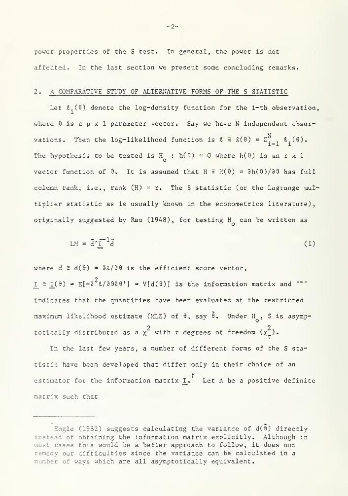
2. A COMPARATIVE STUDY OF ALTERNATIVE FORMS OF THE S STATISTIC
Let £.(9) denote the log-density function for the i-th observation,
where 9 is a p x 1 parameter vector. Say we have N independent obser-
Nvations. Then the log-likelihood function is i = £(9) = E I (9).
The hypothesis to be tested is H : h(9) = where h(9) is an r x 1
vector function of 9. It is assumed that H = H(9) = 3h(9)/39 has full
column rank, i.e., rank (H) r. The S statistic (or the Lagrange mul-
tiplier statistic as is usually known in the econometrics literature)
,
originally suggested by Rao (1948), for testing H can be written as
LM - d'f^d (1)
where d = d(9) = 3.Z./39 is the efficient score vector,
1.= 1(9) = E[-32Z/3939»] = V[d(9)] is the information matrix and
"""
indicates that the quantities have been evaluated at the restricted
maximum likelihood estimate (MLE) of 9, say 9. Under H , S is asymp-
2 2totically distributed as a x with r degrees of freedom (x )•
In the last few years, a number of different forms of the S sta-
tistic have been developed that differ only in their choice of an
estimator for the information matrix _I_. Let A be a positive definite
matrix such that
Engle (1982) suggests calculating the variance of d(9) directlyinstead of obtaining the information matrix explicitly. Although in
most cases this would be a better approach to follow, it does not
remedy our difficulties since the variance can be calculated in a
number of ways which are all asymptotically equivalent.
-3-
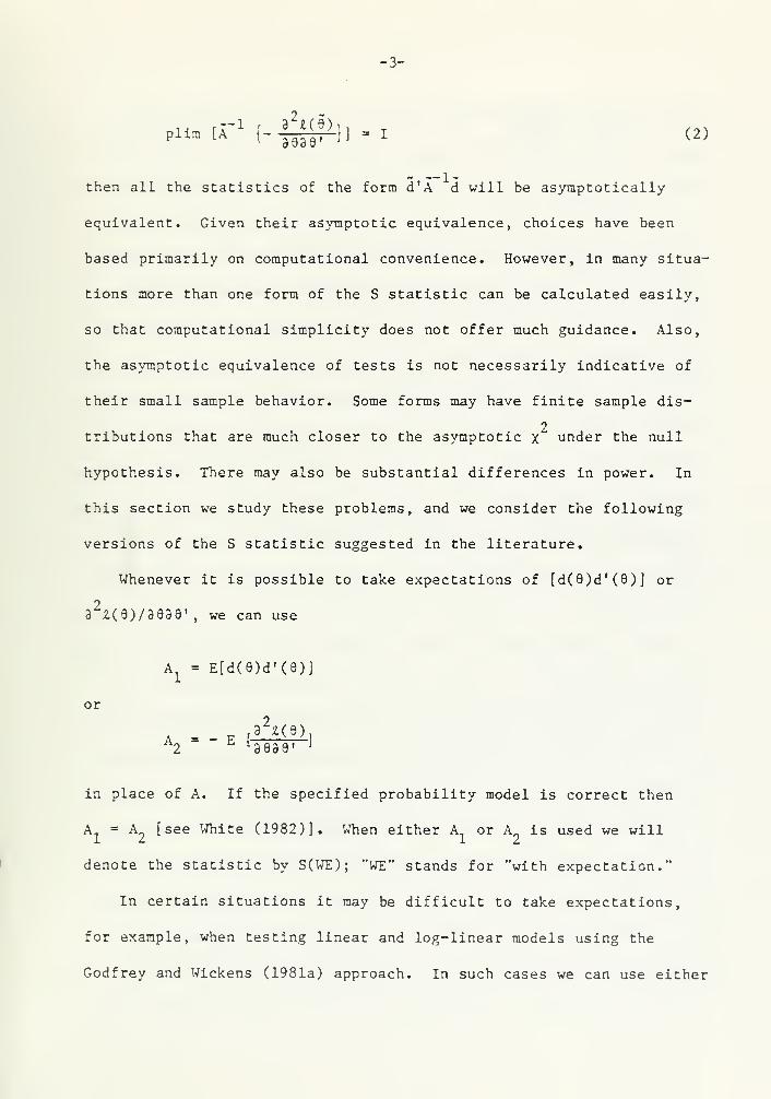
then all the statistics of the form d'A d will be asymptotically
equivalent. Given their asymptotic equivalence, choices have been
based primarily on computational convenience. However, in many situa-
tions more than one form of the S statistic can be calculated easily,
so that computational simplicity does not offer much guidance. Also,
the asymptotic equivalence of tests is not necessarily indicative of
their small sample behavior. Some forms may have finite sample dis-
2tributions that are much closer to the asymptotic x under the null
hypothesis. There may also be substantial differences in power. In
this section we study these problems, and we consider the following
versions of the S statistic suggested in the literature.
Whenever it is possible to take expectations of [d(9)d'(9)j or
32£(9)/3939' , we can use
Ax
= E[d(9)d'(8)J
or
A = - E [lmi
]A2
L 3939* J
in place of A. If the specified probability model is correct then
A = A [see White (1982)]. When either A or A is used we will
denote the statistic by S(WE); "WE" stands for "with expectation."
In certain situations it may be difficult to take expectations,
for example, when testing linear and log-linear models using the
Godfrey and Wickens (1981a) approach. In such cases we can use either
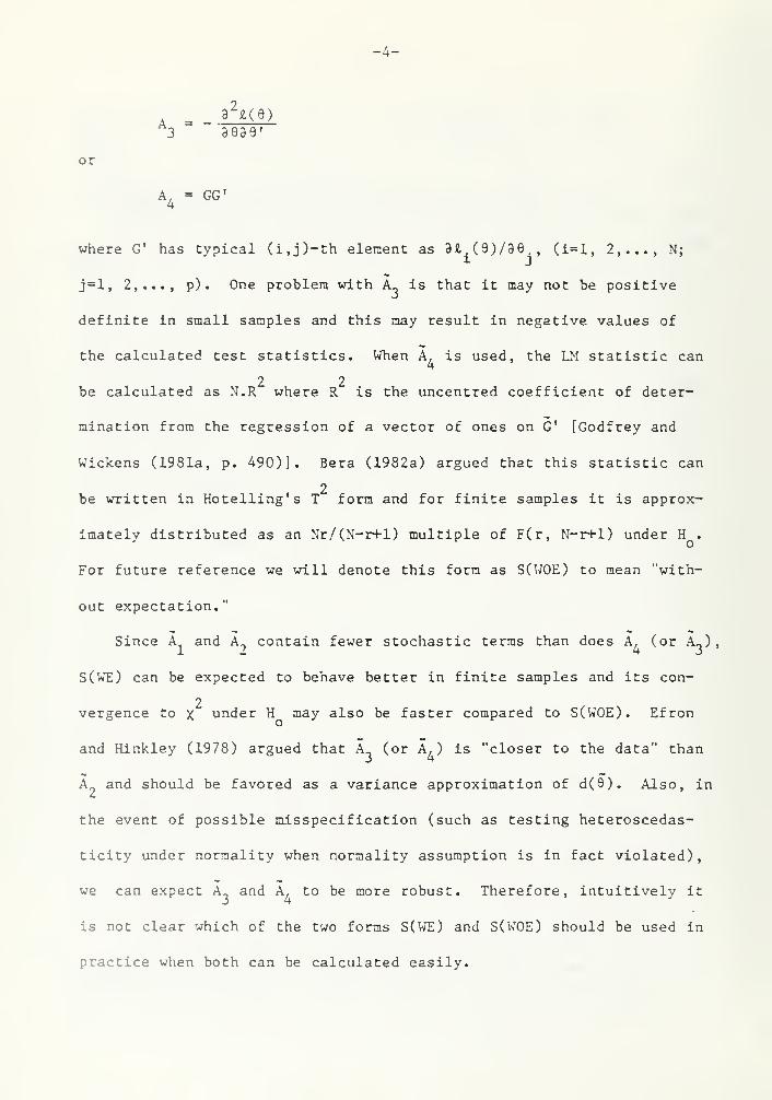
— 4+—
. 32Ji(e)
A„ =
or
3 3999*
A, = GG'4
whe re G' has typical (i,j)-th element as 3£ (9)/36., (i=l, 2,..., N;
j=l, 2,..., p) . One problem with A. is that it may not be positive
definite in small samples and this may result in negative values of
the calculated test statistics. When A, is used, the LM statistic can4
2 2be calculated as N.R where R is the uncentred coefficient of deter-
mination from the regression of a vector of ones on G* [Godfrey and
Wickens (1981a, p. 490)]. Bera (1982a) argued that this statistic can
2be written in Hotelling's T form and for finite samples it is approx-
imately distributed as an Nr/(N-r+l) multiple of F(r, N-r+1) under H .
For future reference we will denote this form as S(WOE) to mean "with-
out expectation."
Since A, and A_ contain fewer stochastic terms than does A. (or A_),12 4 3
S(WE) can be expected to behave better in finite samples and its con-
2vergence to x under H may also be faster compared to S(WOE). Efron
and Hinkley (1978) argued that A (or A.) is "closer to the data" than
A„ and should be favored as a variance approximation of d(9). Also, in
the event of possible misspecif ication (such as testing heteroscedas-
ticity under normality when normality assumption is in fact violated),
we can expect A_ and A, to be more robust. Therefore, intuitively itJ 4
is not clear which of the two forms S(WE) and S(WOE) should be used in
practice when both can be calculated easily.
-5-
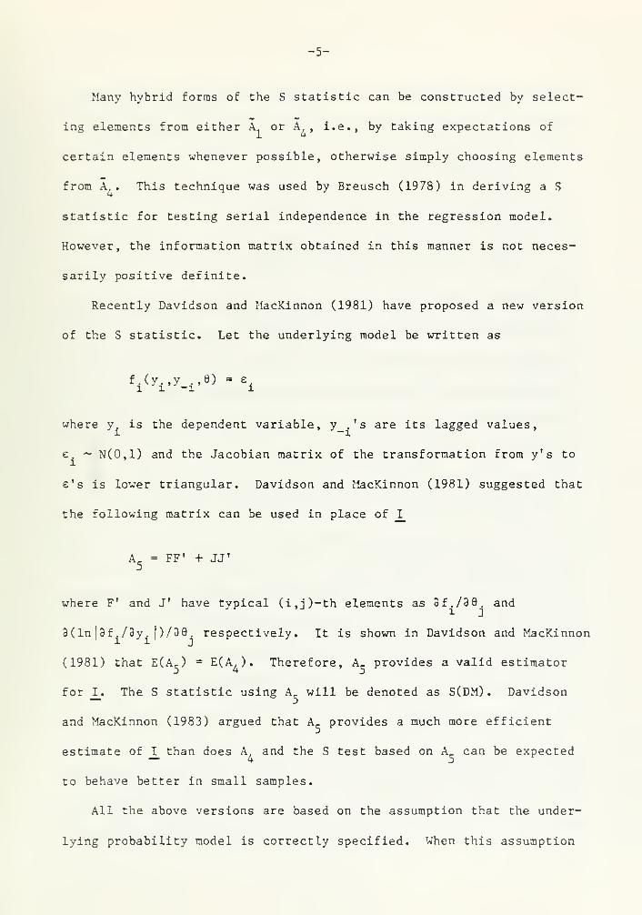
Many hybrid forms of the S statistic can be constructed by select-
ing elements from either /L or A , i.e., by taking expectations of
certain elements whenever possible, otherwise simply choosing elements
from A, . This technique was used by Breusch (1978) in deriving a S4
statistic for testing serial independence in the regression model.
However, the information matrix obtained in this manner is not neces-
sarily positive definite.
Recently Davidson and MacKinnon (1981) have proposed a new version
of the S statistic. Let the underlying model be written as
f.(y.,y .,e) - e,
where y. is the dependent variable, y .'s are its lagged values,
e. ~ N(0,1) and the Jacobian matrix of the transformation from y' s to
e's is lower triangular. Davidson and MacKinnon (1981) suggested that
the following matrix can be used in place of I
A - FF' + JJ'
where F' and J' have typical (i,j)-th elements as 3f./38. and
3 ( In I 3 f . /3y . f)/39. respectively. It is shown in Davidson and MacKinnon1 i i J
(1981) that E(A-) = E(A,). Therefore, A provides a valid estimator
for J_.The S statistic using A will be denoted as S(DM) . Davidson
and MacKinnon (1983) argued that A_ provides a much more efficient
estimate of I than does A, and the S test based on A_ can be expected— 4 5
to behave better in small samples.
All the above versions are based on the assumption that the under-
lying probability model is correctly specified. When this assumption
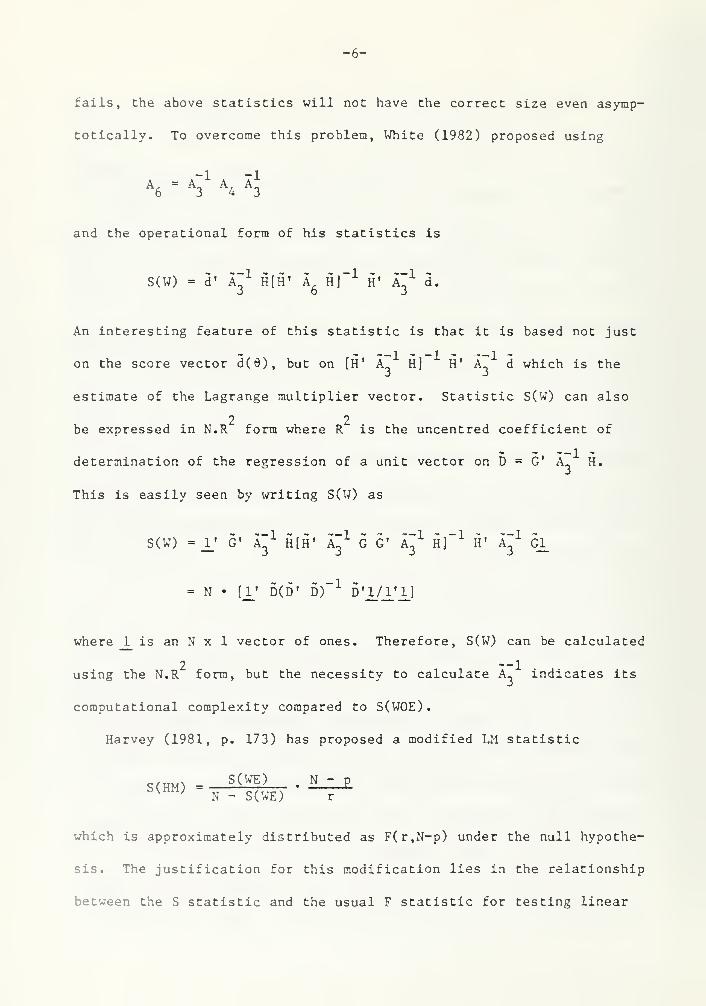
-6-
fails, the above statistics will not have the correct size even asymp-
totically. To overcome this problem, White (1982) proposed using
A6
= A3
A4
A3
and the operational form of his statistics is
S(W) = d' A"1
S[H' A, H]"1
H' A"1
d.Jo J
An interesting feature of this statistic is that it is based not just
— I ~ -i , — i -
on the score vector d(6), but on [H' A H] H' A_ d which is the
estimate of the Lagrange multiplier vector. Statistic S(W) can also
2 2be expressed in N.R form where R is the uncentred coefficient of
determination of the regression of a unit vector on D = G' A H.
This is easily seen by writing S(W) as
s(w) = v g 1 a"1
h[h* a"1
g g' a"1
h]"1
iv a^1
gi
- N • [V 5(5' 5)" 1D'J7J_'_1_]
where _1 is an N x 1 vector of ones. Therefore, S(W) can be calculated
2 —
1
using the N.R form, but the necessity to calculate A_ indicates its
computational complexity compared to S(WOE).
Harvey (1981, p. 173) has proposed a modified LM statistic
S(HM ) =S(UE)
•N - PbkHA)
N - SUE) r
which is approximately distributed as F(r,N-p) under the null hypothe-
sis. The justification for this modification lies in the relationship
between the S statistic and the usual F statistic for testing linear
-7-
restrictions in the linear regression model with normal disturbances.
Kiviet (19S1) reports some simulation results in the context of test-
ing serial independence, suggesting that this modification can lead to
a closer correspondence between the nominal and actual significance
levels.
Davidson and MacKinnon (1983) have examined the small sample per-
formances of S(WOE) and S(DM) for testing linear and log-linear models
within a Box-Cox transformation framework. Their main findings are
2that (i) under the null hypothesis S(DM) is closer to x distribution
in small samples than is S(WOE) and (ii) there is not much difference
in terms of power between these two statistics. We took a different
model for our simulation study since all the above S statistics cannot
be calculated for testing linear and log-linear models. Also we
wanted to have a sufficiently flexible model that permitted the study
of the behavior of all the statistics under different circumstances.
Our study examines the small sample performance of the S statistics
listed above for testing jointly the homoscedasticity (H) and serial
independence (I_) of normal regression disturbances. For the alterna-
tive hypothesis the data were gathered by violating _H, _I_ and normality
(N) as well as their various combinations. This provides us with an
opportunity to compare the performances of the statistics under dif-
ferent situations such as "undertesting" (when the statistic fails to
test all departures that occur), "exact testing" (the situation for
which the statistic is designed) and "overtesting" (when we test for
more departures than actually occur) [for a detailed discussion of
these concepts, see 3era and Jarque (1982)].
-8-
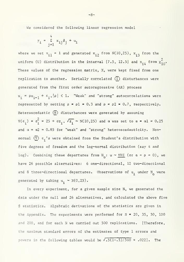
We considered the following linear regression model
4
j - Z x 6 + u.
j-l
where we set x.. = 1 and generated x._ from N(10,25), x _ from the
2uniform (U) distribution in the interval [7.5, 12. 5] and x , from X in
»
These values of the regression matrix, X, were kept fixed from one
replication to another. Serially correlated (I_) disturbances were
generated from the first order autoregressive (AR) process
u. = Pu._, + e.,|p| < 1. "Weak" and "strong" autocorrelations were
represented by setting p = pi = 0.3 and p = p2 = 0.7, respectively.
Heteroscedastic (H_) disturbances were generated by assuming
2 ,
—
V(c.) = o. = 25 + az., /z7 ~ N(10,25) and a was set to a = al = 0.2511 11and a = a2 = 0.85 for "weak" and "strong" heteroscedasticity . Non-
normal (N) e ' s were obtained from the Student's distribution with
five degrees of freedom and the log-normal distribution (say t and
log). Combining these departures from H : u ~ NHI (or a = p =0), we
have 26 possible alternatives: 6 one-directional, 12 two-directional
and 8 three-directional departures. Observations of u. under H were10generated by taking u. ~ N(0,25).
In every experiment, for a given sample size N, we generated the
data under the null and 26 alternatives, and calculated the above five
S statistics. Algebraic derivations of the statistics are given in
the Appendix. The experiments were performed for N = 20, 35, 50, 100
and 200, and for each N we carried out 500 replications. [Therefore,
the maximum standard errors of the estimates of type 1 errors and
powers in the following tables would be /.5( 1-. 5)/500 = .022]. The
_Q-
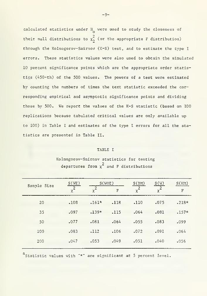
calculated statistics under H were used to study the closeness ofo J
2 .
their null distributions to x9 (° r tne appropriate F distribution)
through the Kolraogorov-Smirnov (K-S) test, and to estimate the type I
errors. These statistics values were also used to obtain the simulated
10 percent significance points which are the appropriate order statis-
tics (450-th) of the 500 values. The powers of a test were estimated
by counting the numbers of times the text statistic exceeded the cor-
responding empirical and asymptotic significance points and dividing
those by 500. We report the values of the K-S statistic (based on 100
replications because tabulated critical values are only available up
to 100) in Table I and estimates of the type I errors for all the sta-
tistics are presented in Table II.
TABLE I
Kolmogorov-Smirnov statistics for testing2
departures from x and F distributions
Sample SizeS(WE)
2X
S(WOE) S(DM)2
X
S(W)
2X
S(HM)2
X F F
20 .108 .161* .118 .110 .075 .218*
35 .097 .139* .115 .064 .081 .157*
50 .077 .081 .064 .055 .083 .099
100 .083 .112 .106 .072 .091 .064
200 .047 .053 .049 .051 .040 .056
Statistic values with "*" are significant at 5 percent level.
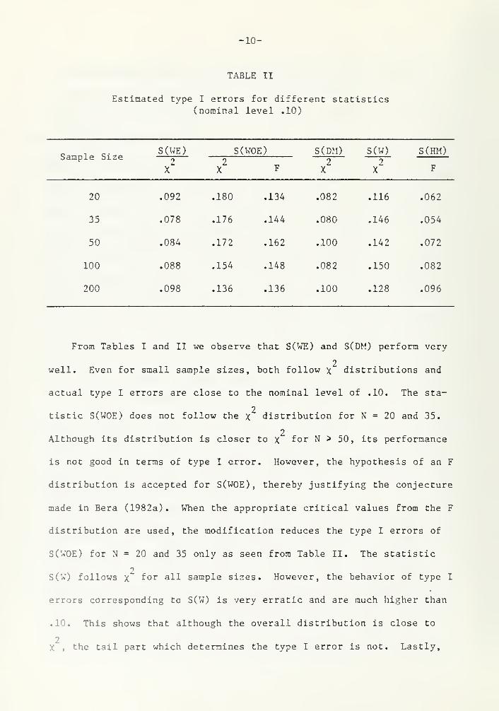
-10-
TABLE II
Estimated type I errors for different statistics(nominal level .10)
Sample SizeS(WE)
2X
S(WOE) S(DM)2
X
S(W)
2X
S(HM)2
X F F
20 .092 .180 .134 .082 .116 .062
35 .078 .176 .144 .080 .146 .054
50 .084 .172 .162 .100 .142 .072
100 .088 .154 .148 .082 .150 .082
200 .098 .136 .136 .100 .128 .096
From Tables I and II we observe that S(WE) and S(DM) perform very
2well. Even for small sample sizes, both follow x distributions and
actual type I errors are close to the nominal level of .10. The sta-
2tistic S(WOE) does not follow the x distribution for N = 20 and 35.
2Although its distribution is closer to x for N > 50, its performance
is not good in terms of type I error. However, the hypothesis of an F
distribution is accepted for S(WOE), thereby justifying the conjecture
made in Bera (1982a). When the appropriate critical values from the F
distribution are used, the modification reduces the type I errors of
S(WOE) for N = 20 and 35 only as seen from Table II. The statistic
2S(W) follows x f° r aH sample sizes. However, the behavior of type I
errors corresponding to S(W) is very erratic and are much higher than
.10. This shows that although the overall distribution is close to
2, the tail part which determines the type I error Is not. Lastly,

-11-
Harvey's correction does not work in our case. This is in contrast to
the results obtained by Kiviet (1981).
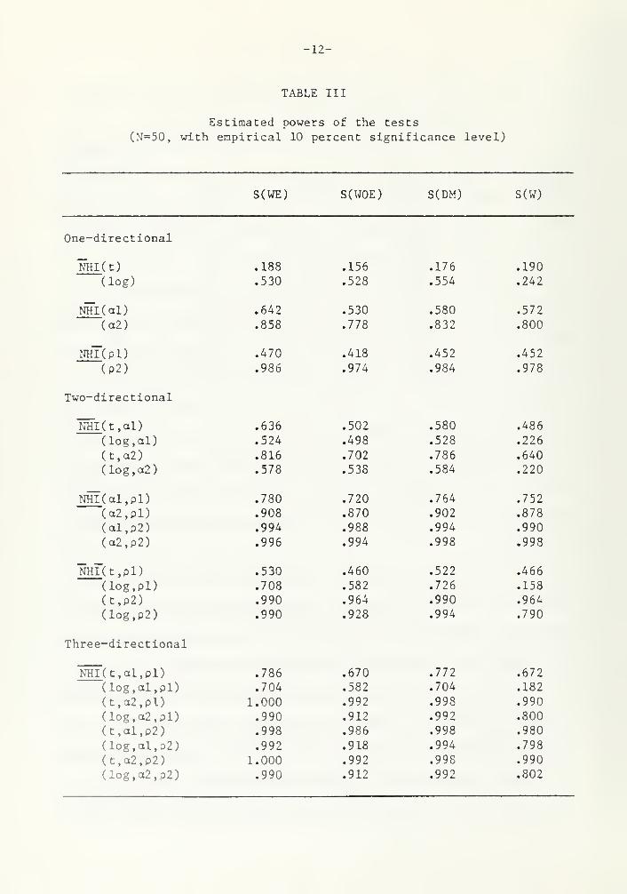
The estimated powers of the tests, calculated using simulated crit-
ical points are presented in Table III for N » 50. Since the behavior
of the tests differs under the null hypothesis, as illustrated in
Tables I and II, any meaningful power comparison requires the use of
estimated (rather than asymptotic) critical values. For S(HM) , esti-
mated powers, using simulated critical points, are the same as those
for S(WE) since the former is a monotonic transformation of the latter,
The left hand column in Table III indicates the characteristics of the
regression disturbances. Recall that pi and p2 denote "weak" and
"strong" first order serial correlation, ctl and a2 denote "weak" and
"strong" heteroscedasticity and, "t" and "log" denote that the errors
e. were obtained from student t and log-normal distributions respec-
tively. So, for example, u ~ NHI (al ,p2) indicates the errors are nor-
mally distributed, "weakly" heteroscedastic and "strongly" serially
correlated.
All the test statistics being investigated are designed to test
the null hypothesis of white noise, homoscedastic and normal distur-
bances (u ~ NHI ) against the alternative of first order serially cor-
related and heteroscedastic but normal errors (u ~ NHI ) . For such
alternatives, on the basis of the relative numerical magnitudes of the
powers, the preference ordering would be S(WE) , S(DM) , S(W) , and
S( T.vOE). Although it should be said that the power differences are not
substantial (maximum power difference between the most powerful and
least powerful test is only 0.06). In the case of overtesting, where
-12-
TABLE III
Estimated powers of the tests
(N=50, with empirical 10 percent significance level)
S(WE) S(WOE) S(DM) S(W)
One-directional
NHI (t)
dog)
NHI (al)
(a2)
nhT(pD(p2)
Two-directional
NHI( t , al
)
(log.al)(t,a2)(log,a2)
NHI (al,pl)(a2,pl)(al,p2)(a2,p2)
NHl"(t,pl)
(log.pl)(t,p2)(log,p2)
Three-directional
.188 .156 .176 .190
.530 .528 .554 .242
.642 .530 .580 .572
.858 .778 .832 .800
.470 .418 .452 .452
.986 .974 .984 .978
.636 .502 .580 .486
.524 .498 .528 .226
.816 .702 .786 .640
.578 .538 .584 .220
.780 .720 .764 .752
.908 .870 .902 .878
.994 .988 .994 .990
.996 .994 .998 .998
.530 .460 .522 .466
.708 .582 .726 .158
.990 .964 .990 .964
.990 .928 .994 .790
NHI(t,al,pl) .786 .670 .772 .672
(log,al,pl) .704 .582 .704 .182
(t,a2,pl) 1.000 .992 .998 .990
(log,o2,pl) .990 .912 .992 .800
(t,al, P 2) .998 .986 .998 .980
(log,al,p2) .992 .918 .994 .798
(t,a2,p2) 1.000 .992 .998 .990
(log,a2,p2) .990 .912 .992 .802
-13-
we test for more departures from the null hypothesis than actually
occur, i.e., u ~ NHI or u ~ NHI , the preference ordering remains the
same. When the underlying assumption of normality is violated, i.e.,
u ~ NHI , u ~ NHI, u ~ NHI or u ~ NHI, some interesting results arise.
For example, when there is undertesting, u ~ NHI , the powers of S(WE)
,
S(WOE) and S(DM) are not adversely affected. However, quite surpris-
ingly, that is not the case for S(W) . It loses substantial power when
the alternative is contaminated by the log-normal distribution. For
example, when u ~ NHI(al ,pl) the power is 0.752 but this falls to
0.182 when u ~ NHI (log,al ,pl) . The power loss is smaller but still
significant for the other log-normal cases. The S(W) statistic
suffers a similar loss of power when the alternative of serially
correlated errors or heteroscedastic errors is contaminated by the
log-normal distribution. The other tests also tend to have lower
power in these cases. For the alternatives u ~ NHI and u ~ NHI , S(WE)
is best followed by S(DM) , S(WOE) and S(W). When the model is com-
pletely misspecif ied , such as when the alternative is NHI , one would
expect S(W) to perform "better" with a power around 0.10 since it is
designed for the case when the probability model is not correctly spec-
ified. For NHI ( t) , the performance of LM(W) and all the other statis-
tics is not good. However, when the alternative is NHI (log) , S(W)'s
performance while still not good is far superior to the other tests.
Similar observations can be made on the power of the tests for N =
20 35 100 and 200. ^n fact > f° r these values of N, S(DM) performs
+
Results corresponding to these values of N are available from theauthors on request.
-14-
marginally better than S(WE). On the basis of the above limited simu-
lation study our recommendation would be to use S(DM) or S(WE) , and
when there is a possibility of raisspecif ication S(W) can be used with
some caution. In certain cases, S(WE) cannot be obtained whereas S(DM)
can be obtained easily, for example, while testing linear and log-
linear models within Box-Cox framework. There are also circumstances
where S(DM) is not applicable such as for specification tests in the
limited dependent variable models [see Bera et al. (1983)]. When both
are available either of them can be used since in terms of type I
error and power there is not much difference among these two versions
of the S test.
3. INVARIANCE OF THE S STATISTIC
A striking feature of the S test is its invariance to different
alternatives. There are many interesting examples of this, but here
we will mention only a few. The S statistic for testing normality
suggested in Bera and Jarque (1981) with the Pearson family of distri-
butions as the alternative, remains unchanged under Gram-Charlier
(type A) alternatives [see Bera (1982b, p. 98)]. Statistics for test-
ing homoscedasticity are invariant to different forms of alternatives
such as multiplicative and additive heteroscedasticity , as has been
noted by Breusch and Pagan (1979) and Godfrey and Wickens (1981b).
Testing serial independence against q-th order autoregressive [AR(q)J
or q-th order moving average [MA(q)] processes lead to the same test
statistic; see for instance, Breusch (1978) and Godfrey (1978).
Pesaran (1979) found that the S test is "incapable of differentiating
-15-
between polynomial lags and rational distributed lags." These exam-
ples raise the question whether the S test will be inferior to other
asymptotically equivalent tests with respect to power since it does
not use precise information of the alternative.
Godfrey (1981) took up this question and compared the powers of
the S and LR tests for local alternatives in the context of testing
serial independence when the alternatives are AR(1) and MA(1) pro-
cesses. Using his analysis it can be shown that AR(1) and MA(1) pro-
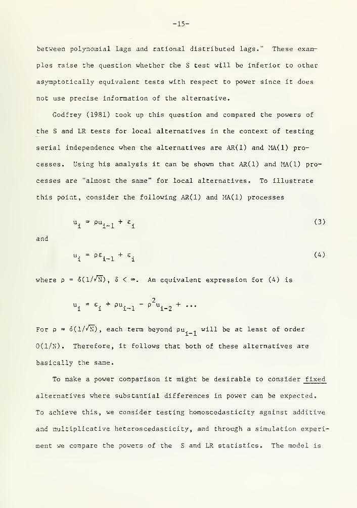
cesses are "almost the same" for local alternatives. To illustrate
this point, consider the following AR(1) and MA(1) processes
and
a - pu e (3)
u. = PVl + e. (4)
where p = 6(1//>T), 5 < ». An equivalent expression for (4) is
ui
= £i+ pU
i-l " p2ui-2
+ •'•
For p = 6(1//n), each term beyond Pu._nwill be at least of order
0(1/N). Therefore, it follows that both of these alternatives are
basically the same.
To make a power comparison it might be desirable to consider fixed
alternatives where substantial differences in power can be expected.
To achieve this, we consider testing horaoscedasticity against additive
and multiplicative heteroscedasticity , and through a simulation experi-
ment we compare the powers of the S and LR statistics. The model is
-16-
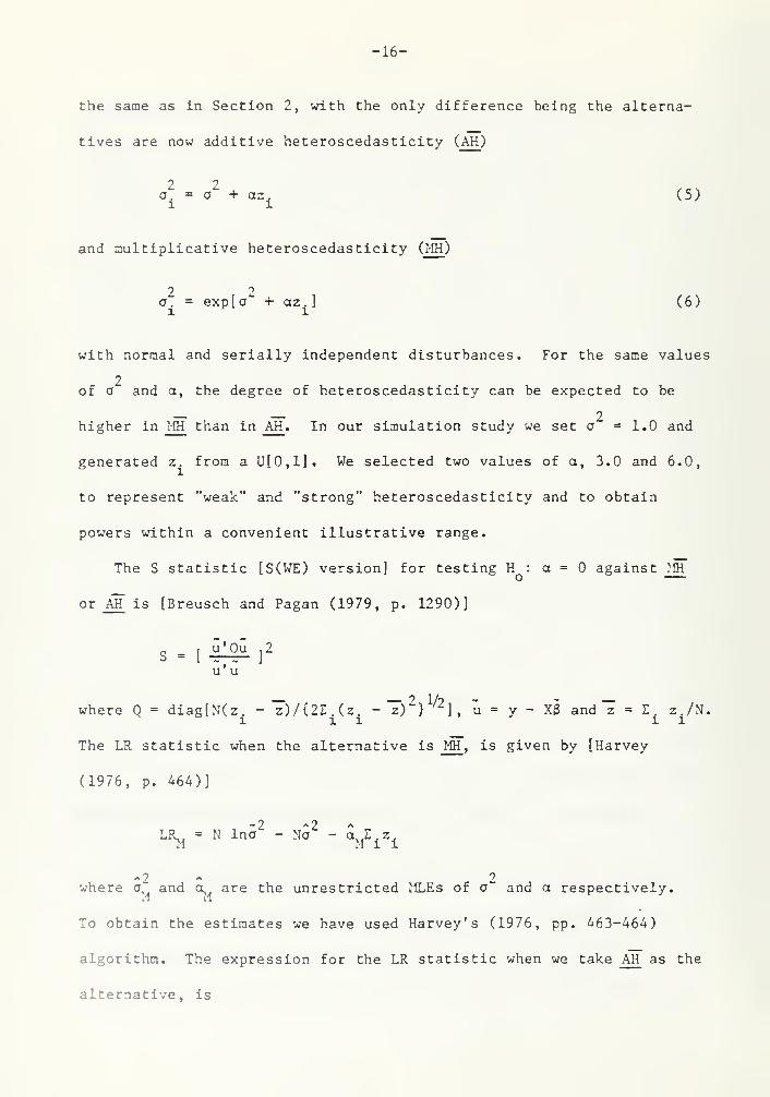
the same as in Section 2, with the only difference being the alterna-
tives are now additive heteroscedasticity (AH )
2 2a. = a + az. (5)i i
and multiplicative heteroscedasticity (MH )
2 2a. = exp[ a + az.
]
(6)
with normal and serially independent disturbances. For the same values
2of a and a, the degree of heteroscedasticity can be expected to be
higher in MH than in AH . In our simulation study we set a = 1.0 and
generated z. from a U[0,1]. We selected two values of a, 3.0 and 6.0,
to represent "weak" and "strong" heteroscedasticity and to obtain
powers within a convenient illustrative range.
The S statistic [S(WE) version] for testing H : a = against MH
or AH is [Breusch and Pagan (1979, p. 1290)]
u' u
where Q = diag[N(z. - 7)/{2Z.(z. - T)2}
fl] , u = y - XS and 7 = Z . z./N.
1 11 11The LR statistic when the alternative is _MH, is given by [Harvey
(1976, p. 464)]
-2 -2...a - NaLR., = N Ina - Ma - a„E , z
"7. 2where a" and a are the unrestricted MLEs of a" and a respectively.
1*1 M
To obtain the estimates we have used Harvey's (1976, pp. 463-464)
algorithm. The expression for the LR statistic when we take AH as the
alternative, is
-17-
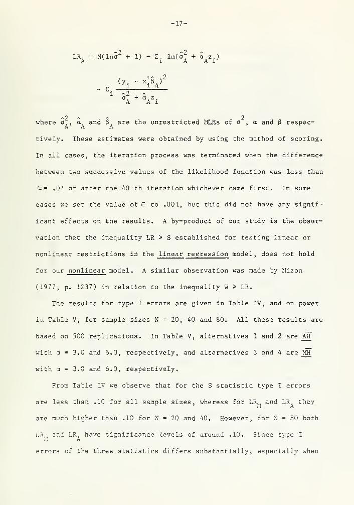
1
LRA
= N(lna + 1) - E. ln(at+ a
Az.)
A i A A l
.( -vi" xiV
2
i -2a. + a z.A A l
where a., a, and 3. are the unrestricted MLEs of a , a and 3 respec-A A A
tively. These estimates were obtained by using the method of scoring.
In all cases, the iteration process was terminated when the difference
between two successive values of the likelihood function was less than
6 = .01 or after the 40-th iteration whichever came first. In some
cases we set the value of € to .001, but this did not have any signif-
icant effects on the results. A by-product of our study is the obser-
vation that the inequality LR > S established for testing linear or
nonlinear restrictions in the linear regression model, does not hold
for our nonlinear model. A similar observation was made by Mizon
(1977, p. 1237) in relation to the inequality W > LR.
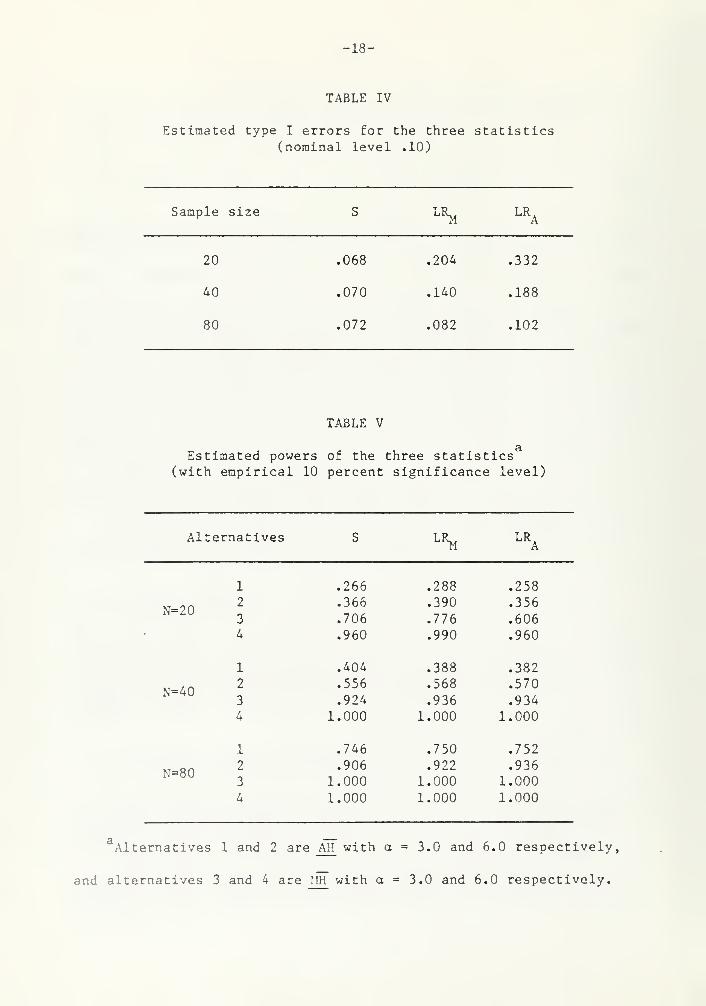
The results for type I errors are given in Table IV, and on power
in Table V, for sample sizes N = 20, 40 and 80. All these results are
based on 500 replications. In Table V, alternatives 1 and 2 are AH
with a = 3.0 and 6.0, respectively, and alternatives 3 and 4 are MH
with a = 3.0 and 6.0, respectively.
From Table IV we observe that for the S statistic type I errors
are less than .10 for all sample sizes, whereas for LR,. and LR, they
are much higher than .10 for N = 20 and 40. However, for N = 80 both
LR,, and LR, have significance levels of around .10. Since type IA A
errors of the three statistics differs substantially, especially when
-18-
TABLE IV
Estimated type I errors for the three statistics(nominal level .10)
Sample size S LR>1
LRA
20 .068 .204 .332
40 .070 .140 .188
80 .072 .082 .102
TABLE V
aEstimated powers of the three statistics
(with empirical 10 percent significance level)
Alternatives S LRM
LRA
1 .266 .288 .258
N=202
3
.366
.706
.390
.776
.356
.6064 .960 .990 .960
1 .404 .388 .382
N=402
3
.556
.924
.568
.936
.570
.934
4 1.000 1.000 1.000
1 .746 .750 .752
N=802
3
.906
1.000.922
1.000.936
1.000
4 1.000 1.000 1.000
aAlternatives 1 and 2 are _AH with a = 3.0 and 6.0 respectively,
and alternatives 3 and 4 are !IH with a = 3.0 and 6.0 respectively.
-19-
the sample size is small, we have used simulated critical points for
calculating power. It is observed from Table V that powers for alter-
natives 3 and 4 are higher than those for alternatives 1 and 2, as
expected. For alternatives 3 and 4, LR,, does better than LR. as oneM A
would expect. However, for alternatives 1 and 2, LR does not alwaysA
have higher power than LR^ . Comparing the powers for S with those for
LR, and LR , it is seen that for N = 20 , the power of S lies betweenA A
the powers of LK^ and LR , and for N = 40 and 80, S has slightly less
power than the other two statistics. Therefore, the S test is effec-
tive in detecting both kinds of heteroscedasticity. Godfrey (1981)
reached to a similar conclusion when he compared the S and LR proce-
dures in the context of testing serial independence against AR(1) and
MA(1) alternatives. These observations show that although the alge-
braic form of the S statistic does not take account of the specific
alternatives, its numerical values do take account of the data.
Therefore, the invariance of the S test to a class of alternatives is
not necessarily a drawback of the procedure. Given the computational
complexities of the LR procedure, the S test may be preferred. More-
over, even though the LR statistic uses specific information concern-
ing the alternative, it does not provide any guidance about the exact
nature of the alternative. For instance, from Table V it is seen that
LR^ ( LRA
) has very high power against aTT(MH). Therefore, if the LR
statistic is found to be significant, we cannot infer much about the
alternative - the same complaint levelled against the S test.

-20-
4. CONCLUSION
In this paper we have studied some of the properties of the S test
procedure. It has been observed that various asymptotically equiva-
lent forms of the S test can have different finite sample properties.
On the basis of the results of Section 2, we recommend the use of S(WE)
and S(DM) versions. We found that the S test has good power to detect
heteroscedasticity per se, in spite of its inability to discriminate
between various forms of the alternative hypothesis..
As an end-note on this paper, we should add that since our conclu-
sions are based on the simulation results they are open to many criti-
cisms. However, in the absence of analytical results, we do feel, our
study sheds further lights on the behavior of the S statistics in
addition to the findings of Davidson and MacKinnon (1983) and Godfrey
(1981). And since our primary interest is the relative performances
of various statistics which have been calculated from the same samples
(and hence are positively correlated), the standard errors of the dif-
ferences of powers can be expected to be less than those of the esti-
mates of powers [see Godfrey (1981, p. 1451)].
-21-
APPENDIX
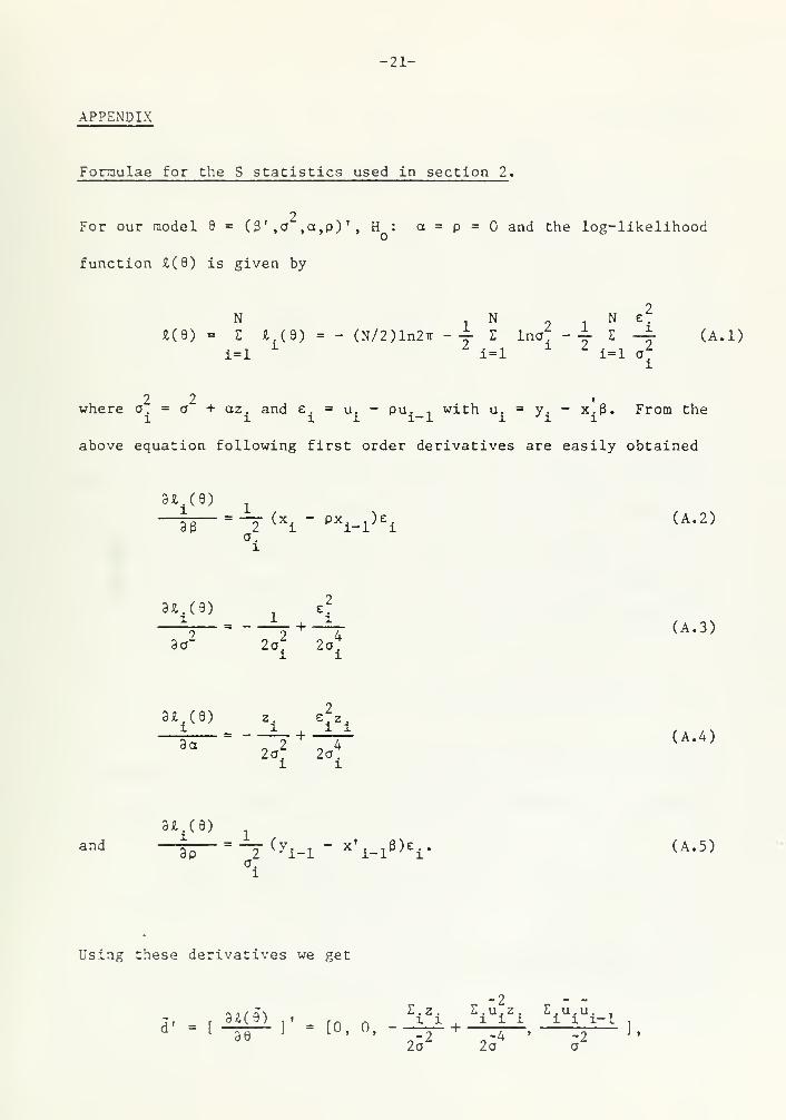
Formulae for the S statistics used in section 2 .
2For our model 9 = (0' ,a ,a,p) f
, H : a = p = and the log-likelihood
function 4(9) is given by
2N N N £7
£(9) = Z £.(9) = - (N/2)ln2ir - i- E lno\ - i- Z -|- (A.l)
i=l1
i=lX Z
i=l afi
2 2 »
where a. = a + az. and e, = u. - pu. , with u. = y. - x.3. From thel l i l l-l l J \ l
above equation following first order derivatives are easily obtained
34.(9) ,
(x. - px. ,)e. (A. 2)33 2
v~iK
i-1 ia.i
34.(3) , e2
i l,ii 2 4
3a 2a? 2ai l
(A. 3)
34,(9) z. eV+-M (A.4)3a
2a2
2a4
i l
34.(9)
and —Tp-
=
"T (yi-l " x'i-l
B)ei*
(A * 5)a.i
Using these derivatives we get
-2« a ,- ^ \ £ . z . Z.u.z. Z.u.u.,
d =1-39— J " 10, 0, "-T2-+ 4 . T2 ''
2a 2a a
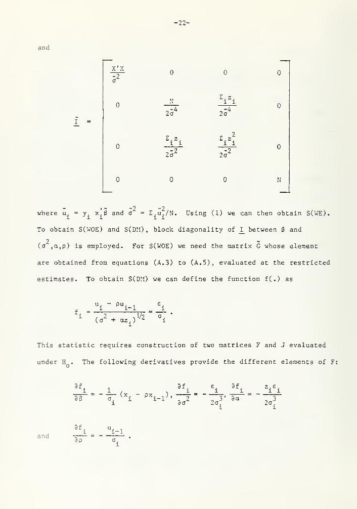
and
-22-
I =
X'X
N
2i"
2.z.1 1
2 a2
254
r 2
-92a""
N
o
where u. = y x.3 and a = S.u./N. Using (1) we can then obtain SCUTO.
To obtain S(WOE) and S(DM) , block diagonality of J_ between and
2(a ,a,p) is employed. For S(WOE) we need the matrix G whose element
are obtained from equations (A. 3) to (A. 5), evaluated at the restricted
estimates. To obtain S(DM) we can define the function f(.) as
f. =1
ui
~ pui-i h
(a2 + a2 .)
V2" °1
This statistic requires construction of two matrices F and J evaluated
under H . The following derivatives provide the different elements of F:
z.e
.
1 13f, , 3f. £. 3f.
1 1 , v _1 X_ 1"
a.^ x
ipx
i-l;
' 2 ' 3* 3a ' 31 do la . 2a
.
1 1
30
and
3fi
~3p~'i-1
-23-
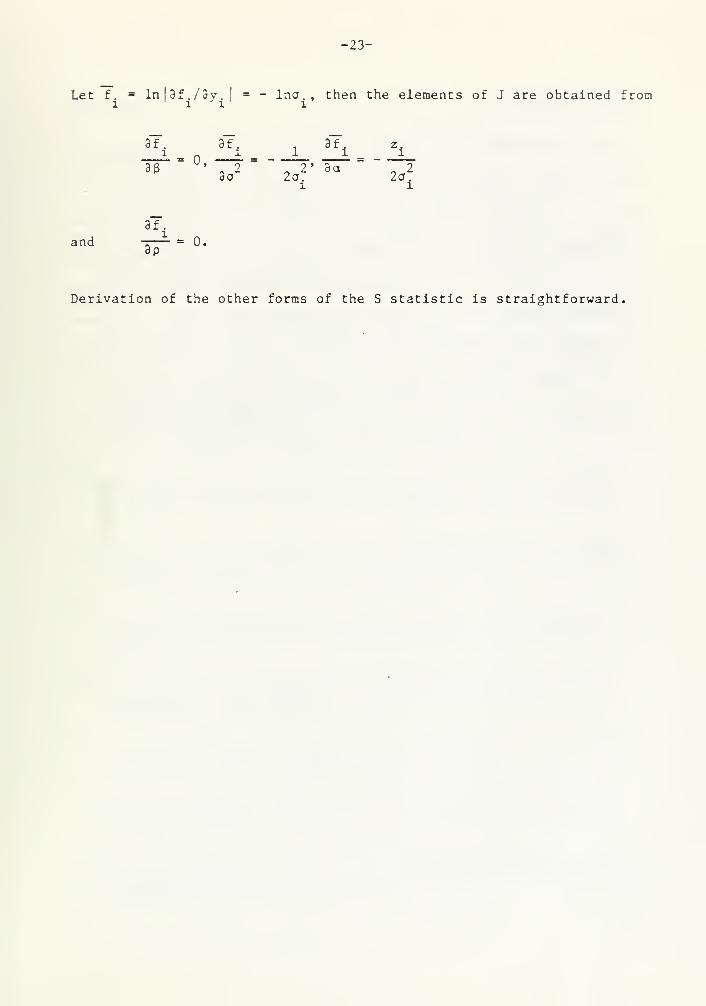
Let f. ln|3f./3v.l = - lna. , then the elements of J are obtained fron1 1 ' 1 i
3~f~. 37. . if. z.—i- o —i- --i 1---L.da za. la,
i i
3fi
and — = 0.3p
Derivation of the other forms of the S statistic is straightforward.

-24-
ACKXOWLEDGEMENTS
We would like to thank Ray Byron, Michael McAleer, Grayham Mizon,
Adrian Pagan, Jean Marie Rolin, Deane Terrell and especially Jan
Kiviet for helpful comments, Russell Davidson and James MacKinnon for
permission to refer to their unpublished paper and helpful suggestions,
Errors, of course, remain our sole responsibility. The second author
gratefully acknowledges the financial support provided by the Japanese
Government's Department of Education and the research support provided
by the Economic Planning Agency. The views and opinions expressed in
this paper are not necessarily those of the Economic Planning Agency.
-25-
REFERENCES
Bera, A. K. (1982a), "A new test for normality," Economics Letters , 9,263-268.
Bera, A. K. (1982b), Aspects of Econometric Modelling , unpublishedPh.D. dissertation, The Australian National University.
Bera, A. K. and C. M. Jarque (1981), "An efficient large-sample test
for normality of observations and regression residuals," WorkingPapers in Economics and Econometrics, N° 040, The AustralianNational University.
Bera, A. K. and C. M. Jarque (1982), "Model specification tests: Asimultaneous approach," Journal of Econometrics , 20 , 59-82.
Bera, A. K. , C. M. Jarque and L. F. Lee (1983), "Testing for the
normality assumption in limited dependent variable models,"International Economic Review , 25 , (forthcoming).
Breusch, T. S. (1978), "Testing for autocorrelation in dynamic linear
models," Australian Economic Papers , 17 , 334-355.
Breusch, T. S. and A. R. Pagan (1979), "A simple test for heterosce-dasticity and random coefficient variation," Econometrica , 47
,
1287-1294.
Davidson, R. and J. G. MacKinnon (1981), "Model specification testsbased on artificial linear regressions," Discussion Paper N° 426,Department of Economics, Queen's University.
Davidson, R. and J. G. MacKinnon (1983), "Small sample properties of
alternative forms of the Lagrange multiplier test," EconomicsLetters , 12 , 269-275.
Efron, B. and D. V. Hinkley (1978), "Assessing the accuracy of the
maximum likelihood estimator: Observed versus expected Fisherinformation," Biometrika , 65 , 457-487.
Engle, R. F. (1982), "A general approach to Lagrange multiplier modeldiagnostics," Journal of Econometrics , 20 , 83-104.
Godfrey, L. G. (1978), "Testing against general autoregressive andmoving average error models when the regressors include laggeddependent variables," Econometrica , 46 , 1293-1302.
Godfrey, L. G. (1981), "On the invariance of the Lagrange multipliertest with respect to certain changes in the alternative hypothesis,Econometrica, 49, 1443-1455.
-26-
Godfrey, L. G. and M. R. Wickens (1981a), "Testing linear and log-linear regressions for functional form," Review of EconomicStudies , 48 , 487-496.
Godfrey, L. G. and M. R. Wickens (1981b), "Tests of misspecif icationusing locally equivalent alternative models," Discussion Paper 66,Department of Economics and Related Studies, University of York.
Harvey, A. C. (1976), "Estimating regression models with multiplicativeheteroscedasticity," Econometrica , 44 , 461-465.
Harvey, A. C. (1981), The Econometric Analysis of Time Series , (Oxford:Philip Allan)
.
Kiviet, J. F. (1981), "On the rigour of some specification tests for
modelling dynamic relationships," Report AE 11/81, Faculty of
Actuarial Science and Econometrics, University of Amsterdam.
Mizon, G. E. (1977), "Inferential procedures in nonlinear models:An application in a UK industrial cross section study of factorsubstitution and return to scale," Econometrica , 45 , 1221-1242.
Pesaran, M. H. (1979), "Diagnostic testing and exact maximum likelihoodestimation of dynamic models," in Proceedings of the EconometricSociety European Meeting , 1979, ed. E. G. Charatsis, (Amsterdam:
North Holland), pp. 63-87.
Rao, C. R. (1948), "Large sample tests of statistical hypothesesconcerning several parameters with applications to problems of
estimation," Proceedings of the Cambridge Philosophical Society,
44 , 50-57.
White, H. (1982), "Maximum likelihood estimation of misspecifiedmodels," Econometrica, 50, 1-25.
D/74
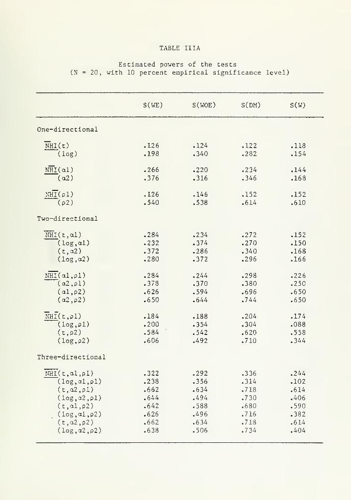
TABLE IIIA
Estimated powers of the tests
(N = 20, with 10 percent empirical significance level)
S(WE) S(WOE) S(DM) S(W)
One-directional
NHI( t)
(log)
NHI( al)(a2)
nhT(pD(P2)
Two-directional
NHI ( t , al
)
(log,al)(t,a2)(log,a2)
NHI( al.pl)(a2,pl)(al,p2)(a2,p2)
KHUt.pl)(log, pi)
(t,p2)(log,p2)
Three-directional
.126 .124 .122 .118
.198 .340 .282 .154
.266 .220 .234 .144
.376 .316 .346 .168
.126 .146 .152 .152
.540 .538 .614 .610
284 .234 .272 .152
232 .374 .270 .150372 .286 .340 .168280 .372 .296 .166
284 .244 .298 .226378 .370 .380 .250
626 .594 .696 .650650 .644 .744 .650
184 .188 .204 .174
200 .354 .304 .088584 .542 .620 .558
606 .492 .710 .344
NHI(t,al,pl) .322 .292 .336 .244
(log,al,pl) .238 .356 .314 .102
(t,a2,pl) .662 .634 .718 .614
(log,a2,pl) .644 .494 .730 .406(t,al, P 2) .642 .588 .680 .590
(log,al, P 2) .626 .496 .716 .382
(t,a2,p2) .662 .634 .718 .614
(log,a2,p2) .638 .506 .734 .404
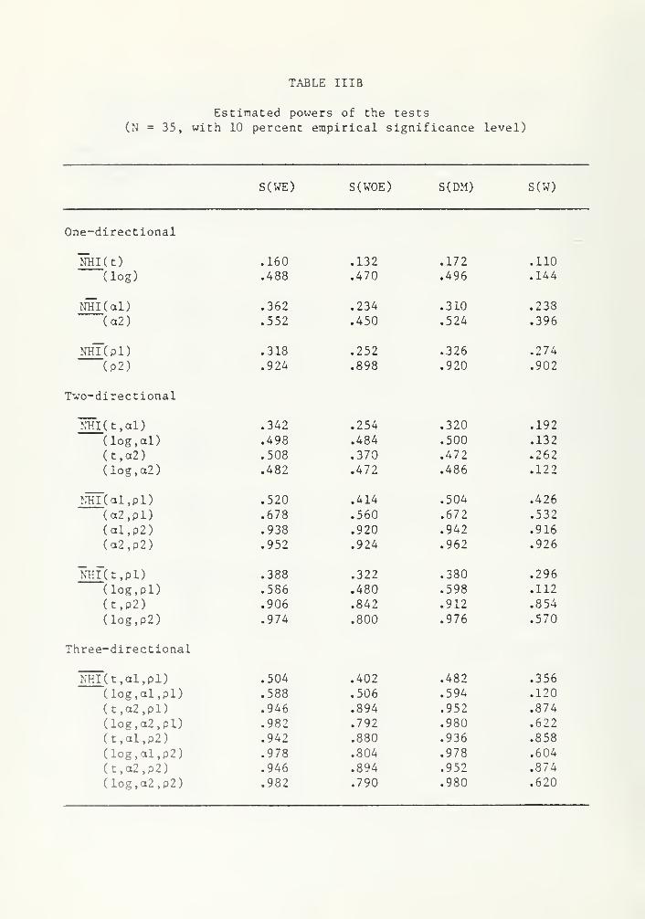
TABLE IIIB
Estimated powers of the tests(N = 35, with 10 percent empirical significance level)
S(WE) S(WOE) S(DM) S(W)
One-directional
NHI (t)
(log)
NHI ( al
)
(a2)
NH~(pl)(P2)
Two-directional
NHI( t,al)(log,al)(t,a2)(log,a2)
NHlC al.pl)(a2,pl)(al,p2)(a2,p2)
~NHl"(t,pl)
(log, pi)(t,p2)
(log,p2)
Three-directional
.160 .132 .172 .110
.488 .470 .496 .144
.362 .234 .310 .238
.552 .450 .524 .396
.318 .252 .326 .274
.924 .898 .920 .902
.342 .254 .320 .192
.498 .484 .500 .132
.508 .370 .472 .262
.482 .472 .486 .122
.520 .414 .504 .426
.678 .560 .672 .532
.938 .920 .942 .916
.952 .924 .962 .926
.388 .322 .380 .296
.586 .480 .598 .112
.906 .842 .912 .854
.974 .800 .976 .570
NHI(t,al,pl) .504 .402 .482 .356
(log,al,pl) .588 .506 .594 .120
(t,a2,pl) .9^6 .894 .952 .874
(log,a2,pl) .982 .792 .980 .622
(t,al,p2) .942 .880 .936 .858
(log,al,p2) .978 .804 .978 .604
(t,a2,p2) .946 .894 .952 .874
(log,a2,p2) .982 .790 .980 .620
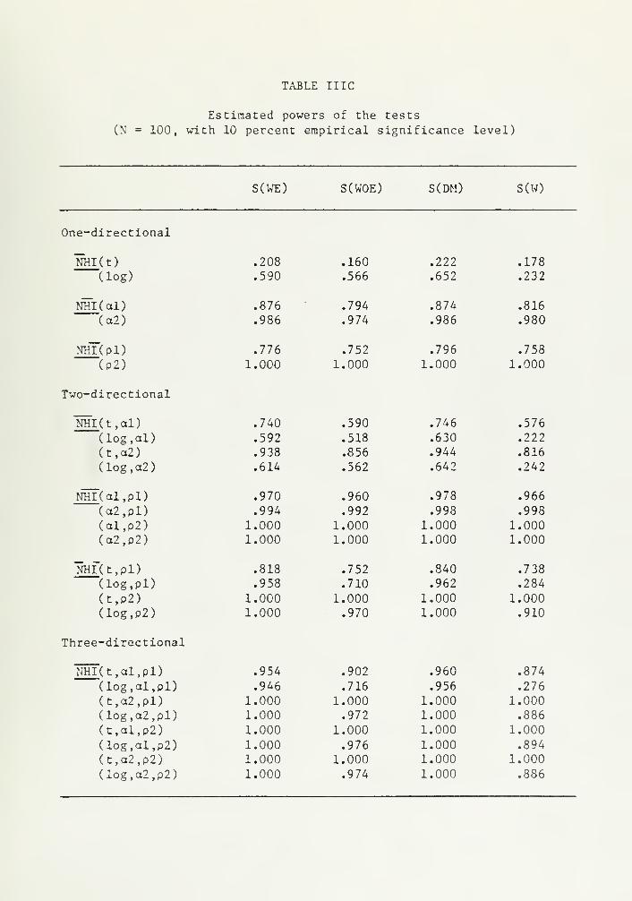
TABLE IIIC
Estimated powers of the tests
(N = 100, with 10 percent empirical significance level)
S(WE) S(WOE) S(DM) S(W)
One-directional
NHI(t)(log)
NTTl(al)
(a2)
nhT(pD(P2)
Two-directional
~NHI (t,al)
(log,al)(t,a2)(log,a2)
NHl"( al.pl)(a2,pl)(al,p2)(o2,p2)
NHI(t,pl)(log, pi)
(t,p2)(log,p2)
Three-directional
.208 .160 .222 .178
.590 .566 .652 .232
.876 .794 .874 .816
.986 .974 .986 .980
.776 .752 .796 .758
1.000 1.000 1.000 1.000
.740 .590 .746 .576
.592 .518 .630 .222
.938 .856 .944 .816
.614 .562 .642 .242
.970 .960 .978 .966
.994 .992 .998 .998
1.000 1.000 1.000 1.0001.000 1.000 1.000 1.000
.818 .752 .840 .738
.958 .710 .962 .284
1.000 1.000 1.000 1.0001.000 .970 1.000 .910
NHI(t,al,pl) .954 .902 .960 .874
(log,al,pl) .946 .716 .956 .276
(t,a2,pl) 1.000 1.000 1.000 1.000Uog,a2,pl) 1.000 .972 1.000 .886
(t,al,p2) 1.000 1.000 1.000 1.000
(log,al,p2) 1.000 .976 1.000 .894
(t,a2,p2) 1.000 1.000 1.000 1.000(log,a2,p2) 1.000 .974 1.000 .886
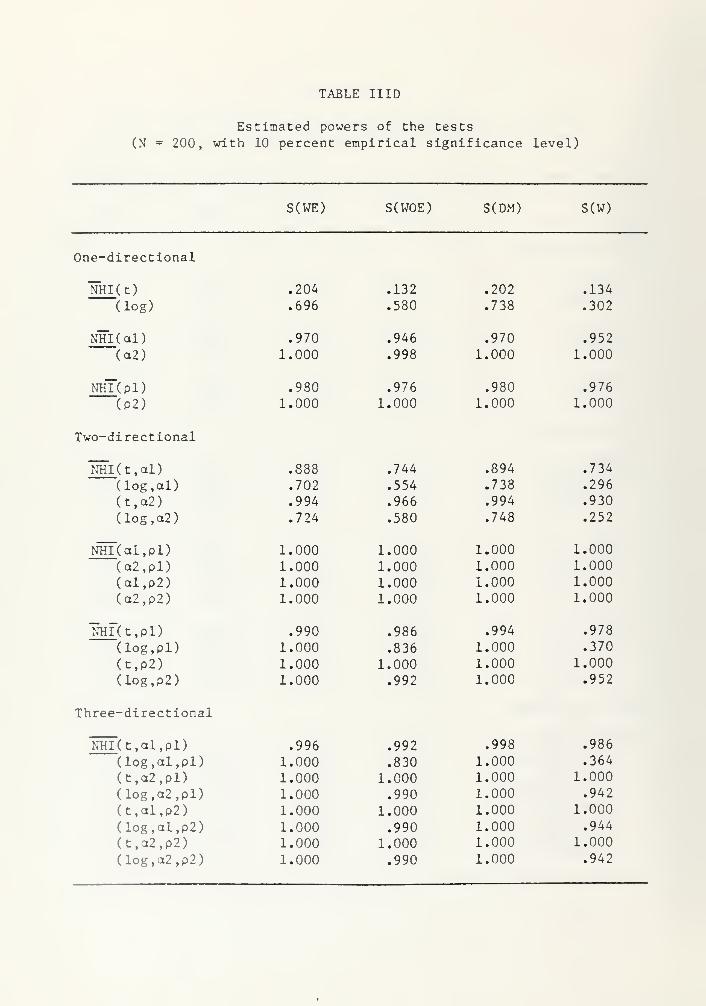
TABLE HID
Estimated powers of the tests
(N = 200, with 10 percent empirical significance level)
S(WE) S(WOE) S(DM) S(W)
One-directional
NHI( t)
(log)
NHI( al)(o2)
nhT(pD(P2)
Two-directional
NHI ( t , ol
)
(log,al)(t,a2)
(log,o2)
NHI( al,pl)(a2,pl)(ol,p2)(a2,p2)
NHI(t,pl)(log, pi)
(t,p2)(log,p2)
Three-directional
.204 .132 .202 .134
.696 .580 .738 .302
.970 .946 .970 .952
1.000 .998 1.000 1.000
.980 .976 .980 .976
1.000 1.000 1.000 1.000
.888 .744 .894 .734
.702 .554 .738 .296
.994 .966 .994 .930
.724 .580 .748 .252
1.000 1.000 1.000 1.000
1.000 1.000 1.000 1.000
1.000 1.000 1.000 1.000
1.000 1.000 1.000 1.000
.990 .986 .994 .978
1.000 .836 1.000 .370
1.000 1.000 1.000 1.000
1.000 .992 1.000 .952
NHI(t,al,pl) .996 .992 .998 .986
(log,al,pl) 1.000 .830 1.000 .364
(t,a2,pl) 1.000 1.000 1.000 1.000
(log,a2,pl) 1.000 .990 1.000 .942
(t,al,p2) 1.000 1.000 1.000 1.000
(log,al,p2) 1.000 .990 1.000 .944
(t,a2,p2) 1.000 1.000 1.000 1.000
(log,a2,p2) 1.000 .990 1.000 .942


I
1ECKMAN3INDERY INC.
JUN95* N MANCHESTER.
emi -To-Ha* INDIANA 46962