Embed Size (px)
Citation preview
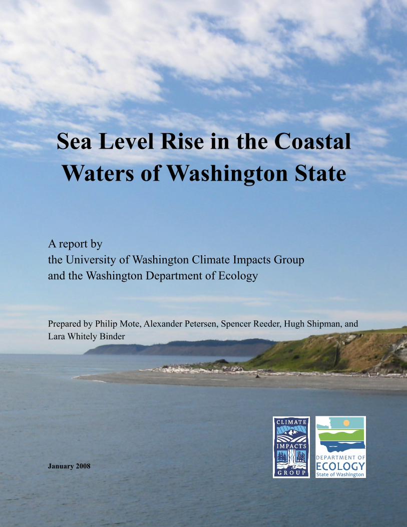
Sea Level Rise in the Coastal Waters of Washington State
A report by the University of Washington Climate Impacts Group and the Washington Department of Ecology
Prepared by Philip Mote, Alexander Petersen, Spencer Reeder, Hugh Shipman, and Lara Whitely Binder
January 2008
CONTENTS
................................................................................................................................1. Background 4.......................................................................................2. Observed rates of global sea level rise 4
...........................................................................................................3. Sea level rise projections 4...............................................................................................................3.1 Thermal expansion 4
......................................................................................................3.2 Cryospheric contribution 5..............................................................................................3.3 Local atmospheric circulation 6
.....................................................................................................3.4 Local tectonic movement 7............................................................4. Synthesis: Summary and calculation of SLR projections 9
.................................................................................5. Unknowns and additional considerations 10......................................................................................................................................References 11
The authors would like to thank the following persons who reviewed this report: Jim Simmonds, Supervi-sor for Water Quality and Quantity, and Angela Grout, Oceanographer, for King County, Washington; Dr. Ian Joughin, University of Washington Polar Science Center; Ray Weldon, Professor, University of Ore-gon; and Susan Tonkin, Coastal Engineer, Moffatt & Nichol. In addition, we wish to thank Dr. Tim Mel-bourne, Associate Professor, Andrew Miner, Researcher, and Marcelo Santillan, Scientific Programmer and GPS Data Analyst, Central Washington University, for providing Figure 8.
Note: Units less than centimeters (cm) are not converted into English units. Centimeter conversions to inches are rounded to the nearest whole unit for ease of reading.
Photo: Whidbey Island near Fort Casey. Photo by Philip Mote.
2
This publication is partially funded by the Joint Institute for the Study of the Atmosphere and Ocean (JISAO) under NOAA Cooperative Agreement No. NA17RJ1232, Contribution # 1474.
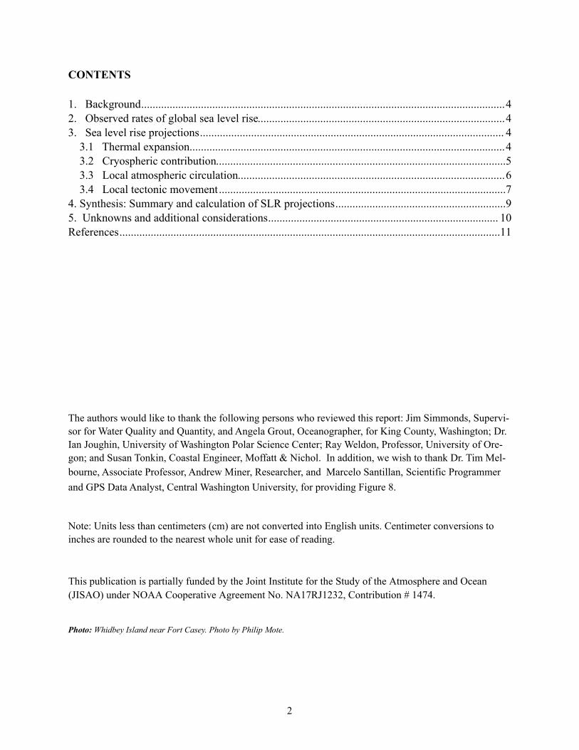
Summary. Local sea level rise (SLR) is produced by the combined effects of global sea level rise and local factors such as vertical land deformation (e.g., tectonic movement, isostatic rebound) and seasonal ocean elevation changes due to atmospheric circulation effects. In this document we re-view available projections of these factors for the coastal wa-ters of Washington and provide low, medium, and high esti-mates of local SLR for 2050 and 2100.
The fourth Assessment Report of the Intergovernmental Panel on Climate Change (IPCC) projects global SLR over the course of this century to be between 18 and 38 cm (7-15”) for their lowest emissions scenario, and between 26 and 59 cm (10-23”) for their highest emissions scenario. Based on the current science, our “medium” estimate of 21st century SLR in Washington is that in Puget Sound, local SLR will closely match global SLR. On the northwest Olympic Peninsula, very little relative SLR will be apparent due to rates of local tectonic uplift that currently exceed pro-jected rates of global SLR. On the central and southern Washington coast, the number of continuous monitoring sites with sufficiently long data records is small, adding to the un-certainty of SLR estimates for this region. Available data points suggest, however, that uplift is occurring in this region, but at rates lower than that observed on the NW Olympic Penin-sula.
The application of SLR estimates in decision making will depend on location, time frame, and risk toler-ance. For decisions with long timelines and low risk tolerance, such as coastal development and public infrastructure, users should consider low-probability high-impact estimates that take into account, among other things, the potential for higher rates of SLR driven by recent observations of rapid ice loss in Green-land and Antarctica, which though observed were not factored into the IPCC’s latest global SLR esti-mates. Combining the IPCC high emissions scenario with 1) higher estimates of ice loss from Green-land and Antarctica, 2) seasonal changes in atmospheric circulation in the Pacific, and 3) vertical land deformation, a low-probability high-impact estimate of local SLR for the Puget Sound Basin is 55 cm (22”) by 2050 and 128 cm (50”) by 2100. Low-probability, high impact estimates are smaller for the central and southern Washington coast (45 cm [18”] by 2050 and 108 cm [43”] by 2100), and even lower for the NW Olympic Peninsula (35 cm [14”] by 2050 and 88 cm [35”] by 2100) due to tectonic up-lift (see Table III). The authors intend to continue investigating the factors contributing to local SLR and will provide updates to this report.
3
Projected sea level rise in Washington’s wa-ters relative to 1980-99, in inches. Shading roughly indicates likelihood.
Sea Level Rise Summary Figure:
3”
6”
30”
50”
2050 2100
13”
40”
20”
10”
6”
1. BackgroundSea level rise (SLR) is increasingly being
considered by private and public entities when making decisions about the placement and pro-tection of structures near shorelines. The Cli-mate Impacts Group (CIG) at University of Washington has recently received inquiries from several municipalities, consultants, and private citizens concerning the likely rates of SLR at specific locations in the waters of Washington State during the 21st century. This document is intended to address those questions and to provide guidance on the use of SLR projections.
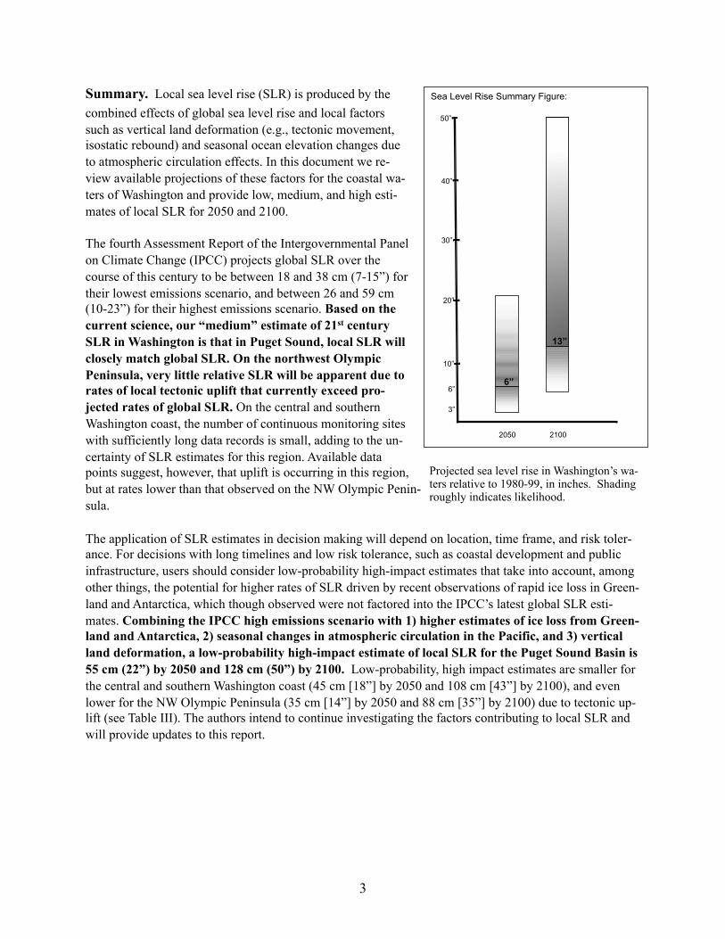
2. Observed rates of global sea level riseGlobal estimates of SLR (Figure 1) can be derived
by considering tide gauge records in combination with models or actual measurements of Earth’s local tec-tonic movement. The average rate of global SLR for 1961-2003 is 1.8 ± 0.5 mm/yr (IPCC SPM, 2007). Satellite altimetry measurements by the TOPEX/Poseidon and Jason 1 satellites covering the years 1993-2003 provide a value of 3.1 ± 0.7 mm/yr (IPCC 2007, Nerem et al. 2006).
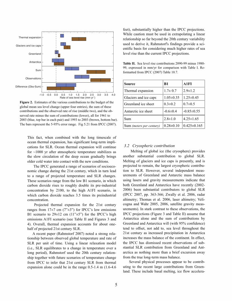
Table I shows the estimated contribution of various processes to observed SLR during those two time periods. The agreement between the sum of contributions and the observed change in SLR is substantially better for the 1993-2003 period than for the 1961-2003 period, and the difference between the sum and the observed change is no longer statistically significant. This convergence is due
Table I. SLR contributions in mm/yr, from IPCC 2007 (Table 5.3). See also Figure 2.
Source 1961-2003 1993-2003
Thermal expansion 0.42 ± 0.12 1.6 ± 0.5
Glaciers and ice caps 0.5 ± 0.18 0.77 ± 0.22
Greenland ice sheet 0.05 ± 0.12 0.21 ± 0.07
Antarctic ice sheet 0.14 ± 0.41 0.21 ± 0.35
Sum 1.1 ± 0.5 2.8 ± 0.7
Observed 1.8 ± 0.5 3.1 ± 0.7
Difference 0.7 ± 0.7 0.3 ± 1.0
mainly to improvements in data collection tech-niques. For the 1993-2003 period, the largest term (and the largest increase from the previous era) is the thermal expansion term.
3. Sea level rise projectionsFour main drivers of local SLR are (1) global
SLR (Table II and Figure 3) driven by the thermal expansion of the ocean; (2) global SLR driven by the melting of land-based ice; (3) local dynamical SLR driven by changes in wind, which push coastal waters toward or away from shore; and (4) local dynamical SLR driven by local movement of the land itself, due primarily to tectonic forces. We now discuss each of these factors. Changes related to the storage of sur-face water in reservoirs and aquifers are estimated to be substantially smaller than the other terms and thus are not discussed.
3.1 Thermal expansionThe ocean has absorbed roughly 80% of the
heating of the climate system associated with rising greenhouse gases during the past ~50 years (IPCC SPM 2007), leading to substantial ocean warming. Because seawater expands slightly when warmed, the volume of the ocean has increased and the ocean is expected to continue expanding as a result of pro-jected increases in 21st century global temperature.
4
Figure 1. Annual averages of the global mean sea level (mm). The red curve shows reconstructed sea level fields since 1870, the blue curve shows coastal tide gauge measurements since 1950, and the black curve is based on satellite altimetry. Error bars show 90% confidence inter-vals. Figure 5.13 from IPCC (2007).
410
Observations: Oceanic Climate Change and Sea Level Chapter 5
The TAR chapter on sea level change provided
estimates of climate and other anthropogenic
contributions to 20th-century sea level rise, based
mostly on models (Church et al., 2001). The
sum of these contributions ranged from –0.8 to
2.2 mm yr–1, with a mean value of 0.7 mm yr–1,
and a large part of this uncertainty was due to the
lack of information on anthropogenic land water
change. For observed 20th-century sea level rise,
based on tide gauge records, Church et al. (2001)
adopted as a best estimate a value in the range of 1
to 2 mm yr–1, which was more than twice as large as
the TAR’s estimate of climate-related contributions.
It thus appeared that either the processes causing
sea level rise had been underestimated or the rate
of sea level rise observed with tide gauges was
biased towards higher values.
Since the TAR, a number of new results have
been published. The global coverage of satellite
altimetry since the early 1990s (TOPography
EXperiment (TOPEX)/Poseidon and Jason) has
improved the estimate of global sea level rise and
has revealed the complex geographical patterns
of sea level change in open oceans. Near-global
ocean temperature data for the last 50 years have
been recently made available, allowing the first observationally
based estimate of the thermal expansion contribution to sea
level rise in past decades. For recent years, better estimates of
the land ice contribution to sea level are available from various
observations of glaciers, ice caps and ice sheets.
In this section, we summarise the current knowledge of
present-day sea level rise. The observational results are assessed,
followed by our current interpretation of these observations in
terms of climate change and other processes, and ending with a
discussion of the sea level budget (Section 5.5.6).
5.5.2 Observations of Sea Level Changes
5.5.2.1 20th-Century Sea Level Rise from Tide Gauges
Table 11.9 of the TAR listed several estimates for global and
regional 20th-century sea level trends based on the Permanent
Service for Mean Sea Level (PSMSL) data set (Woodworth
and Player, 2003). The concerns about geographical bias in
the PSMSL data set remain, with most long sea level records
stemming from the NH, and most from continental coastlines
rather than ocean interiors. Based on a small number (~25) of
high-quality tide gauge records from stable land regions, the
rate of sea level rise has been estimated as 1.8 mm yr–1 for the
past 70 years (Douglas, 2001; Peltier, 2001), and Miller and
Douglas (2004) find a range of 1.5 to 2.0 mm yr–1 for the 20th
century from 9 stable tide gauge sites. Holgate and Woodworth
(2004) estimated a rate of 1.7 ± 0.4 mm yr–1 sea level change
averaged along the global coastline during the period 1948 to
2002, based on data from 177 stations divided into 13 regions.
Church et al. (2004) (discussed further below) determined
a global rise of 1.8 ± 0.3 mm yr–1 during 1950 to 2000, and
Church and White (2006) determined a change of 1.7 ±
0.3 mm yr–1 for the 20th century. Changes in global sea level
as derived from analyses of tide gauges are displayed in Figure
5.13. Considering the above results, and allowing for the
ongoing higher trend in recent years shown by altimetry (see
Section 5.5.2.2), we assess the rate for 1961 to 2003 as 1.8 ±
0.5 mm yr–1 and for the 20th century as 1.7 ± 0.5 mm yr–1.
While the recently published estimates of sea level rise over
the last decades remain within the range of the TAR values
(i.e., 1–2 mm yr–1), there is an increasing opinion that the best
estimate lies closer to 2 mm yr–1 than to 1 mm yr–1. The lower
bound reported in the TAR resulted from local and regional
studies; local and regional rates may differ from the global
mean, as discussed below (see Section 5.5.2.5).
A critical issue concerns how the records are adjusted for
vertical movements of the land upon which the tide gauges
are located and of the oceans. Trends in tide gauge records are
corrected for GIA using models, but not for other land motions.
The GIA correction ranges from about 1 mm yr–1 (or more) near
to former ice sheets to a few tenths of a millimetre per year in
the far field (e.g., Peltier, 2001); the error in tide-gauge based
global average sea level change resulting from GIA is assessed
as 0.15 mm yr–1. The TAR mentioned the developing geodetic
technologies (especially the Global Positioning System; GPS)
that hold the promise of measuring rates of vertical land
movement at tide gauges, no matter if those movements are
due to GIA or to other geological processes. Although there
has been some model validation, especially for GIA models,
systematic problems with such techniques, including short data
spans, have yet to be fully resolved.
Figure 5.13. Annual averages of the global mean sea level (mm). The red curve shows reconstructed sea level fields since 1870 (updated from Church and White, 2006); the blue curve shows coastal tide gauge measurements since 1950 (from Holgate and Woodworth, 2004) and the black curve is based on satellite altimetry (Leuliette et al., 2004). The red and blue curves are deviations from their averages for 1961 to 1990, and the black curve is the deviation from the average of the red curve for the period 1993 to 2001. Error bars show 90% confidence intervals.
This fact, when combined with the long timescale of ocean thermal expansion, has significant long-term impli-cations for SLR. Ocean thermal expansion will continue for ~1000 yr after atmospheric temperature stabilizes as the slow circulation of the deep ocean gradually brings older cold water into contact with the new conditions.
The IPCC generated a range of scenarios of socioeco-nomic change during the 21st century, which in turn lead to a range of projected temperature and SLR changes. These scenarios range from the low B1 scenario, in which carbon dioxide rises to roughly double its pre-industrial concentration by 2100, to the high A1FI scenario, in which carbon dioxide reaches 3.5 times its preindustrial concentration.
Projected thermal expansion for the 21st century ranges from 17±7 cm (7”±3”) for IPCC’s low emissions B1 scenario to 29±12 cm (11”±5”) for the IPCC’s high emissions A1FI scenario (see Table II and Figures 3 and 4). Overall, thermal expansion accounts for about one-half of projected 21st century SLR.
A recent paper (Rahmstorf 2007) noted a strong rela-tionship between observed global temperature and rate of SLR per unit of time. Using a linear relaxation model (i.e., SLR equilibrates to a change in temperature over a long period), Rahmstorf used the 20th century relation-ship together with future scenarios of temperature change from IPCC to infer that 21st century SLR from thermal expansion alone could be in the range 0.5-1.4 m (1.6-4.6
feet), substantially higher than the IPCC projections. While caution must be used in extrapolating a linear relationship so far beyond the 20th century variability used to derive it, Rahmstorf's findings provide a sci-entific basis for considering much higher rates of sea level rise than the current IPCC projections.
Table II. Sea level rise contributions 2090-99 minus 1980-99, expressed in mm/yr for comparison with Table I. Re-formatted from IPCC (2007) Table 10.7.
Source B1 A1FI
Thermal expansion 1.7± 0.7 2.9±1.2
Glaciers and ice caps 1.05±0.35 1.25±0.45
Greenland ice sheet 0.3±0.2 0.7±0.5
Antarctic ice sheet -0.6±0.4 -0.85±0.55
Sum 2.8±1.0 4.25±1.65
Sum (meters per century) 0.28±0.10 0.425±0.165
3.2 Cryospheric contribution Melting of global ice (the cryosphere) provides
another substantial contribution to global SLR. Melting of glaciers and ice caps is presently, and is projected to remain, the largest cryospheric contribu-tion to SLR. However, several independent meas-urements of Greenland and Antarctic mass balance using lasers and gravity measurements indicate that both Greenland and Antarctica have recently (2002-2006) been substantial contributors to global SLR (IPCC 2007, pp. 363-366; Zwally et al. 2006, radar altimetry; Thomas et al. 2006, laser altimetry; Veli-cogna and Wahr 2005, 2006, satellite gravity meas-urements). In stark contrast to these observations, the IPCC projections (Figure 3 and Table II) assume that Antarctica alone and the sum of contributions by Greenland and Antarctica will (with 95% confidence) tend to offset, not add to, sea level throughout the 21st century as increased precipitation in Antarctica increases the mass balance of the continent. In effect, the IPCC has dismissed recent observations of sub-stantial SLR contribution from Greenland and Ant-arctica as nothing more than a brief excursion away from the true long-term mass balance.
Several physical processes appear to be contrib-uting to the recent large contributions from Green-land. These include basal melting, ice flow accelera-
5
419
Chapter 5 Observations: Oceanic Climate Change and Sea Level
and –1.9 to +1.0 mm yr–1 for 1990. However, indirect evidence
from considering other contributions to the sea level budget
(see Section 5.5.6) suggests that the land contribution either is
small (<0.5 mm yr–1) or is compensated for by unaccounted or
underestimated contributions.
5.5.6 Total Budget of the Global Mean Sea Level Change
The various contributions to the budget of sea level change
are summarised in Table 5.3 and Figure 5.21 for 1961 to 2003
and 1993 to 2003. Some terms known to be small have been
omitted, including changes in atmospheric water vapour and
climate-driven change in land water storage (Section 5.5.5),
permafrost and sedimentation (see, e.g., Church et al., 2001),
which very likely total less than 0.2 mm yr–1. The poorly known
anthropogenic contribution from terrestrial water storage (see
Section 5.5.5.4) is also omitted.
For 1961 to 2003, thermal expansion accounts for only
23 ± 9% of the observed rate of sea level rise. Miller and
Douglas (2004) reached a similar conclusion by computing
steric sea level change over the past 50 years in three oceanic
regions (northeast Pacific, northeast Atlantic and western
Atlantic); they found it to be too small by about a factor of
three to account for the observed sea level rise based on nine
tide gauges in these regions. They concluded that sea level rise
in the second half of the 20th century was mostly due to water
mass added to the oceans. However, Table 5.3 shows that the
sum of thermal expansion and contributions from land ice is
smaller by 0.7 ± 0.7 mm yr–1 than the observed global average
sea level rise. This is likely to be a significant difference. The
assessment of Church et al. (2001) could allow this difference
to be explained by positive anthropogenic terms (especially
groundwater mining) but these are expected to have been
outweighed by negative terms (especially impoundment). We
conclude that the budget has not yet been closed satisfactorily.
Given the large temporal variability in the rate of sea level rise
evaluated from tide gauges (Section 5.5.2.4 and Figure 5.17),
the budget is rather problematic on decadal time scales. The
thermosteric contribution has smaller variability (though still
substantial; Section 5.5.3) and there is only moderate temporal
correlation between the thermosteric rate and the tide gauge
rate. The difference between them has to be explained by ocean
mass change. Because the thermosteric and climate-driven land
water contributions are negatively correlated (Section 5.5.5.3.),
Table 5.3. Estimates of the various contributions to the budget of global mean sea level change for 1961 to 2003 and 1993 to 2003 compared with the observed rate of rise. Ice sheet mass loss of 100 Gt yr–1 is equivalent to 0.28 mm yr–1 of sea level rise. A GIA correction has been applied to observations from tide gauges and altimetry. For the sum, the error has been calculated as the square root of the sum of squared errors of the contributions. The thermosteric sea level changes are for the 0 to 3,000 m layer of the ocean.
Sea Level Rise (mm yr–1) Source 1961–2003 1993–2003 Reference
Thermal Expansion 0.42 ± 0.12 1.6 ± 0.5 Section 5.5.3
Glaciers and Ice Caps 0.50 ± 0.18 0.77 ± 0.22 Section 4.5
Greenland Ice Sheet 0.05 ± 0.12 0.21 ± 0.07 Section 4.6.2
Antarctic Ice Sheet 0.14 ± 0.41 0.21 ± 0.35 Section 4.6.2
Sum 1.1 ± 0.5 2.8 ± 0.7
Observed 1.8 ± 0.5 Section 5.5.2.1
3.1 ± 0.7 Section 5.5.2.2
Difference (Observed –Sum) 0.7 ± 0.7 0.3 ± 1.0
Figure 5.21. Estimates of the various contributions to the budget of the global mean sea level change (upper four entries), the sum of these contributions and the observed rate of rise (middle two), and the observed rate minus the sum of contributions (lower), all for 1961 to 2003 (blue) and 1993 to 2003 (brown). The bars represent the 90% error range. For the sum, the error has been calculated as the square root of the sum of squared errors of the contributions. Likewise the errors of the sum and the observed rate have been combined to obtain the error for the difference.
Figure 2. Estimates of the various contributions to the budget of the global mean sea level change (upper four entries), the sum of these contributions and the observed rate of rise (middle two), and the ob-served rate minus the sum of contributions (lower), all for 1961 to 2003 (blue, top bar in each pair) and 1993 to 2003 (brown, bottom bar). The bars represent the 5-95% error range. Fig 5.21 from IPCC (2007).
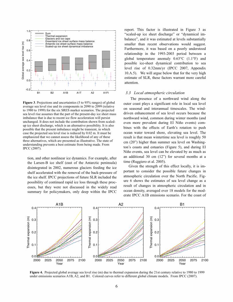
tion, and other nonlinear ice dynamics. For example, after the Larsen-B ice shelf (east of the Antarctic peninsula) disintegrated in 2002, numerous glaciers feeding the ice shelf accelerated with the removal of the back-pressure of the ice shelf. IPCC projections of future SLR included the possibility of continued rapid ice loss through these proc-esses, but they were not discussed in the widely read summary for policymakers, only deep within the IPCC
report. This factor is illustrated in Figure 3 as “scaled-up ice sheet discharge” or “dynamical im-balance”, and it was estimated at levels substantially smaller than recent observations would suggest. Furthermore, it was based on a poorly understood relationship in the 1993-2003 period between a global temperature anomaly 0.63°C (1.1°F) and possible ice-sheet dynamical contribution to sea level rise of 0.32mm/yr (IPCC 2007, Appendix 10.A.5). We will argue below that for the very high estimate of SLR, these factors warrant more careful attention.
3.3 Local atmospheric circulationThe presence of a northward wind along the
outer coast plays a significant role in local sea level on seasonal and interannual timescales. The wind-driven enhancement of sea level occurs because the northward wind, common during winter months (and even more prevalent during El Niño events) com-bines with the effects of Earth’s rotation to push ocean water toward shore, elevating sea level. The result is that mean wintertime sea level is roughly 50 cm (20”) higher than summer sea level on Washing-ton’s coasts and estuaries (Figure 5), and during El Niño events, sea level can be elevated by as much as an additional 30 cm (12”) for several months at a time (Ruggiero et al. 2005).
Given the strength of this effect locally, it is im-portant to consider the possible future changes in atmospheric circulation over the North Pacific. Fig-ure 6 shows the estimates of sea level change as a result of changes in atmospheric circulation and in ocean density, averaged over 18 models for the mod-erate IPCC A1B emissions scenario. For the coast of
6
821
Chapter 10 Global Climate Projections
In all scenarios, the average rate of rise during the 21st century
is very likely to exceed the 1961 to 2003 average rate of 1.8 ± 0.5
mm yr–1 (see Section 5.5.2.1). The central estimate of the rate
of sea level rise during 2090 to 2099 is 3.8 mm yr–1 under A1B,
which exceeds the central estimate of 3.1 mm yr–1 for 1993 to
2003 (see Section 5.5.2.2). The 1993 to 2003 rate may have a
contribution of about 1 mm yr–1 from internally generated or
naturally forced decadal variability (see Sections 5.5.2.4 and
9.5.2). These sources of variability are not predictable and not
included in the projections; the actual rate during any future
decade might therefore be more or less than the projected rate
by a similar amount. Although simulated and observed sea level
rise agree reasonably well for 1993 to 2003, the observed rise
for 1961 to 2003 is not satisfactorily explained (Section 9.5.2),
as the sum of observationally estimated components is 0.7 ± 0.7
mm yr–1 less than the observed rate of rise (Section 5.5.6). This
indicates a deficiency in current scientific understanding of sea
level change and may imply an underestimate in projections.
For an average model (the central estimate for each scenario),
the scenario spread (from B1 to A1FI) in sea level rise is only
0.02 m by the middle of the century. This is small because of the
time-integrating effect of sea level rise, on which the divergence
among the scenarios has had little effect by then. By 2090 to
2099 it is 0.15 m.
In all scenarios, the central estimate for thermal expansion
by the end of the century is 70 to 75% of the central estimate for
the sea level rise. In all scenarios, the average rate of expansion
Figure 10.33. Projections and uncertainties (5 to 95% ranges) of global average sea level rise and its components in 2090 to 2099 (relative to 1980 to 1999) for the six SRES marker scenarios. The projected sea level rise assumes that the part of the present-day ice sheet mass imbalance that is due to recent ice flow acceleration will persist unchanged. It does not include the contribution shown from scaled-up ice sheet discharge, which is an alternative possibility. It is also possible that the present imbalance might be transient, in which case the projected sea level rise is reduced by 0.02 m. It must be emphasized that we cannot assess the likelihood of any of these three alternatives, which are presented as illustrative. The state of understanding prevents a best estimate from being made.
during the 21st century is larger than central
estimate of 1.6 mm yr–1 for 1993 to 2003
(Section 5.5.3). Likewise, in all scenarios the
average rate of mass loss by G&IC during
the 21st century is greater than the central
estimate of 0.77 mm yr–1 for 1993 to 2003
(Section 4.5.2). By the end of the century,
a large fraction of the present global G&IC
mass is projected to have been lost (see, e.g.,
Table 4.3). The G&IC projections are rather
insensitive to the scenario because the main
uncertainties come from the G&IC model.
Further accelerations in ice flow of the
kind recently observed in some Greenland
outlet glaciers and West Antarctic ice streams
could increase the ice sheet contributions
substantially, but quantitative projections
cannot be made with confidence (see Section
10.6.4.2). The land ice sum in Table 10.7
includes the effect of dynamical changes in
the ice sheets that can be simulated with a
continental ice sheet model (Section 10.6.4.2).
It also includes a scenario-independent term
of 0.32 ± 0.35 mm yr–1 (0.035 ± 0.039 m in
110 years). This is the central estimate for
1993 to 2003 of the sea level contribution
from the Antarctic Ice Sheet, plus half of that
from Greenland (Sections 4.6.2.2 and 5.5.5.2). We take this as
an estimate of the part of the present ice sheet mass imbalance
that is due to recent ice flow acceleration (Section 4.6.3.2), and
assume that this contribution will persist unchanged.
We also evaluate the contribution of rapid dynamical
changes under two alternative assumptions (see, e.g., Alley et
al., 2005b). First, the present imbalance might be a rapid short-
term adjustment, which will diminish during coming decades.
We take an e-folding time of 100 years, on the basis of an
idealised model study (Payne et al., 2004). This assumption
reduces the sea level rise in Table 10.7 by 0.02 m. Second,
the present imbalance might be a response to recent climate
change, perhaps through oceanic or surface warming (Section
10.6.4.2). No models are available for such a link, so we assume
that the imbalance might scale up with global average surface
temperature change, which we take as a measure of the magnitude
of climate change (see Appendix 10.A). This assumption adds
0.1 to 0.2 m to the estimated upper bound for sea level rise
depending on the scenario (Table 10.7). During 2090 to 2099,
the rate of scaled-up antarctic discharge roughly balances the
increased rate of antarctic accumulation (SMB). The central
estimate for the increased antarctic discharge under the SRES
scenario A1FI is about 1.3 mm yr–1, a factor of 5 to 10 greater
than in recent years, and similar to the order-of-magnitude
upper limit of Section 10.6.4.2. It must be emphasized that we
cannot assess the likelihood of any of these three alternatives,
which are presented as illustrative. The state of understanding
prevents a best estimate from being made.
Figure 3. Projections and uncertainties (5 to 95% ranges) of global average sea level rise and its components in 2090 to 2099 (relative to 1980 to 1999) for the six SRES marker scenarios. The projected sea level rise assumes that the part of the present-day ice sheet mass imbalance that is due to recent ice flow acceleration will persist unchanged. It does not include the contribution shown from scaled-up ice sheet discharge, which is an alternative possibility. It is also possible that the present imbalance might be transient, in which case the projected sea level rise is reduced by 0.02 m. It must be emphasized that we cannot assess the likelihood of any of these three alternatives, which are presented as illustrative. The state of understanding prevents a best estimate from being made. From IPCC (2007).
Figure 4. Projected global average sea level rise (m) due to thermal expansion during the 21st century relative to 1980 to 1999 under emissions scenarios A1B, A2, and B1. Colored curves refer to different global climate models. From IPCC (2007).
812
Global Climate Projections Chapter 10
10.6 Sea Level Change in the 21st Century
10.6.1 Global Average Sea Level Rise Due to Thermal Expansion
As seawater warms up, it expands, increasing the volume
of the global ocean and producing thermosteric sea level rise
(see Section 5.5.3). Global average thermal expansion can be
calculated directly from simulated changes in ocean temperature.
Results are available from 17 AOGCMs for the 21st century
for SRES scenarios A1B, A2 and B1 (Figure 10.31), continuing
from simulations of the 20th century. One ensemble member
was used for each model and scenario. The time series are rather
smooth compared with global average temperature time series,
because thermal expansion reflects heat storage in the entire
ocean, being approximately proportional to the time integral of
temperature change (Gregory et al., 2001).
During 2000 to 2020 under scenario SRES A1B in the
ensemble of AOGCMs, the rate of thermal expansion is 1.3 ±
0.7 mm yr–1, and is not significantly different under A2 or B1.
This rate is more than twice the observationally derived rate
of 0.42 ± 0.12 mm yr–1 during 1961 to 2003. It is similar to
the rate of 1.6 ± 0.5 mm yr–1 during 1993 to 2003 (see Section
5.5.3), which may be larger than that of previous decades partly
because of natural forcing and internal variability (see Sections
5.5.2.4, 5.5.3 and 9.5.2). In particular, many of the AOGCM
experiments do not include the influence of Mt. Pinatubo, the
omission of which may reduce the projected rate of thermal
expansion during the early 21st century.
During 2080 to 2100, the rate of thermal expansion is
projected to be 1.9 ± 1.0, 2.9 ± 1.4 and 3.8 ± 1.3 mm yr–1 under
scenarios SRES B1, A1B and A2 respectively in the AOGCM
ensemble (the width of the range is affected by the different
numbers of models under each scenario). The acceleration is
caused by the increased climatic warming. Results are shown
for all SRES marker scenarios in Table 10.7 (see Appendix
10.A for methods). In the AOGCM ensemble, under any given
SRES scenario, there is some correlation of the global average
temperature change across models with thermal expansion
and its rate of change, suggesting that the spread in thermal
expansion for that scenario is caused both by the spread in
surface warming and by model-dependent ocean heat uptake
efficiency (Raper et al., 2002; Table 8.2) and the distribution of
added heat within the ocean (Russell et al., 2000).
10.6.2 Local Sea Level Change Due to Change in Ocean Density and Dynamics
The geographical pattern of mean sea level relative to the
geoid (the dynamic topography) is an aspect of the dynamical
balance relating the ocean’s density structure and its circulation,
which are maintained by air-sea fluxes of heat, freshwater
and momentum. Over much of the ocean on multi-annual
time scales, a good approximation to the pattern of dynamic
topography change is given by the steric sea level change, which
can be calculated straightforwardly from local temperature
and salinity change (Gregory et al., 2001; Lowe and Gregory,
2006). In much of the world, salinity changes are as important
as temperature changes in determining the pattern of dynamic
topography change in the future, and their contributions can
be opposed (Landerer et al., 2007; and as in the past, Section
5.5.4.1). Lowe and Gregory (2006) show that in the UKMO-
HadCM3 AOGCM, changes in heat fluxes are the cause of many
of the large-scale features of sea level change, but freshwater
Figure 10.31. Projected global average sea level rise (m) due to thermal expansion during the 21st century relative to 1980 to 1999 under SRES scenarios A1B, A2 and B1. See Table 8.1 for model descriptions.
western North America, the sum of these contri-butions in the annual mean is about 2-3 cm (about 1”) below the global average.
CIG has analyzed over 30 scenarios from global climate models (Mote et al. 2007) and the mean changes in wintertime northward wind are indeed minimal. Consequently, we subtract 1 and 2 cm (less than 1”) from the “very low” SLR estimates for 2050 and 2100, respectively, and consider this component to be negligible for the “medium” SLR estimate. However, several models produce increases in northward wind in wintertime of sufficient strength to add as much as 15 cm (6”) to mean sea level for 2050-2099 compared with 1950-1999, so for the “very high” SLR estimate we add 15 cm (6”).
3.4 Local tectonic movementDirect measurements of sea level at tide
gauges are difficult to interpret because tide gauges record the difference between local sea level and local land level, with interannual variability and measurement uncertainty clouding the picture. Differ-ences in rates of sea level rise can be substantial. For example, the linear trend in sea level for 1973-2000 was 2.82±1.05 mm/yr at Toke Point (Willapa Bay, southern coast) and 1.39±0.94 mm/yr at Cherry Point (near Bel-lingham; Zervas 2001). Without additional evidence it is difficult to separate sea level rise from local land level change, which itself could be caused by a variety of fac-tors including tectonic movement or soil compaction. Trends also change over time: 50-year trends at Seattle
(1898-2000) range from 1.04 mm/yr to 2.80 mm/yr (ibid). Linear trends are influenced by fluctuation in annual and decadal rates of global sea level rise as well as variations in the rate of local vertical land movement (VLM). Deducing the contribution of local VLM formerly required a model of Earth's crustal movement. Recently, direct measurements of sea level from satellites, and of land move-ment from global positioning system (GPS) sensors, have improved our understanding of these two contributions to tide gage meas-urements of sea level.
Crustal deformation associated with plate tectonics and isostatic rebound (adjustments to the disappearance of the great ice sheets) pro-
duces local vertical land movement. Western Wash-ington sits on the edge of the North American conti-nental plate, under which the Juan de Fuca oceanic plate is subducting. This subduction tends to produce uplift in the western extent of the region over time (although historically, large subduction zone earth-quakes of magnitude > 8.0 in the region have resulted in sudden land subsidence of 1 meter (3.3 ft) or more [Leonard et al. 2004, Jacoby et al. 1997]).
7
Figure 6. Local sea level change (m) due to ocean density and circulation change relative to the global average (i.e., positive values indicate greater local sea level change than global) during the 21st century, calculated as the differ-ence between averages for 2080 to 2099 and 1980 to 1999, as an ensemble mean over 16 AOGCMs forced with the SRES A1B scenario. Stippling de-notes regions where the magnitude of the multi-model ensemble mean divided by the multi-model standard deviation exceeds 1.0. From IPCC (2007).
813
Chapter 10 Global Climate Projections
flux change dominates the North Atlantic and momentum flux
change has a signature in the north and low-latitude Pacific and
the Southern Ocean.
Results are available for local sea level change due to ocean
density and circulation change from AOGCMs in the multi-
model ensemble for the 20th century and the 21st century.
There is substantial spatial variability in all models (i.e., sea
level change is not uniform), and as the geographical pattern of
climate change intensifies, the spatial standard deviation of local
sea level change increases (Church et al., 2001; Gregory et al.,
2001). Suzuki et al. (2005) show that, in their high-resolution
model, enhanced eddy activity contributes to this increase, but
across models there is no significant correlation of the spatial
standard deviation with model spatial resolution. This section
evaluates sea level change between 1980 to 1999 and 2080 to
2099 projected by 16 models forced with SRES scenario A1B.
(Other scenarios are qualitatively similar, but fewer models
are available.) The ratio of spatial standard deviation to global
average thermal expansion varies among models, but is mostly
within the range 0.3 to 0.4. The model median spatial standard
deviation of thermal expansion is 0.08 m, which is about 25%
of the central estimate of global average sea level rise during
the 21st century under A1B (Table 10.7).
The geographical patterns of sea level change from different
models are not generally similar in detail, although they have
more similarity than those analysed in the TAR by Church et al.
(2001). The largest spatial correlation coefficient between any
pair is 0.75, but only 25% of correlation coefficients exceed
0.5. To identify common features, an ensemble mean (Figure
10.32) is examined. There are only limited areas where the
model ensemble mean change exceeds the inter-model standard
deviation, unlike for surface air temperature change (Section
10.3.2.1).
Like Church et al. (2001) and Gregory et al. (2001), Figure
10.32 shows smaller than average sea level rise in the Southern
Ocean and larger than average in the Arctic, the former possibly
due to wind stress change (Landerer et al., 2007) or low
thermal expansivity (Lowe and Gregory, 2006) and the latter
due to freshening. Another obvious feature is a narrow band of
pronounced sea level rise stretching across the southern Atlantic
and Indian Oceans and discernible in the southern Pacific. This
could be associated with a southward shift in the circumpolar
front (Suzuki et al., 2005) or subduction of warm anomalies
in the region of formation of sub antarctic mode water (Banks
et al., 2002). In the zonal mean, there are maxima of sea level
rise in 30°S to 45°S and 30°N to 45°N. Similar indications are
present in the altimetric and thermosteric patterns of sea level
change for 1993 to 2003 (Figure 5.15). The model projections
do not share other aspects of the observed pattern of sea level
rise, such as in the western Pacific, which could be related to
interannual variability.
Figure 10.32. Local sea level change (m) due to ocean density and circulation change relative to the global average (i.e., positive values indicate greater local sea level change than global) during the 21st century, calculated as the difference between averages for 2080 to 2099 and 1980 to 1999, as an ensemble mean over 16 AOGCMs forced with the SRES A1B scenario. Stippling denotes regions where the magnitude of the multi-model ensemble mean divided by the multi-model standard deviation exceeds 1.0.
Monthly Mean Sea Level
2005 Jan Apr Jul Oct 2006 Jan Apr Jul Oct 2007 Jan Apr Jul Oct2.0
2.2
2.4
2.6
2.8
3.0
3.2
3.4
m
La Push: 0.48m
Toke Point: 0.62m
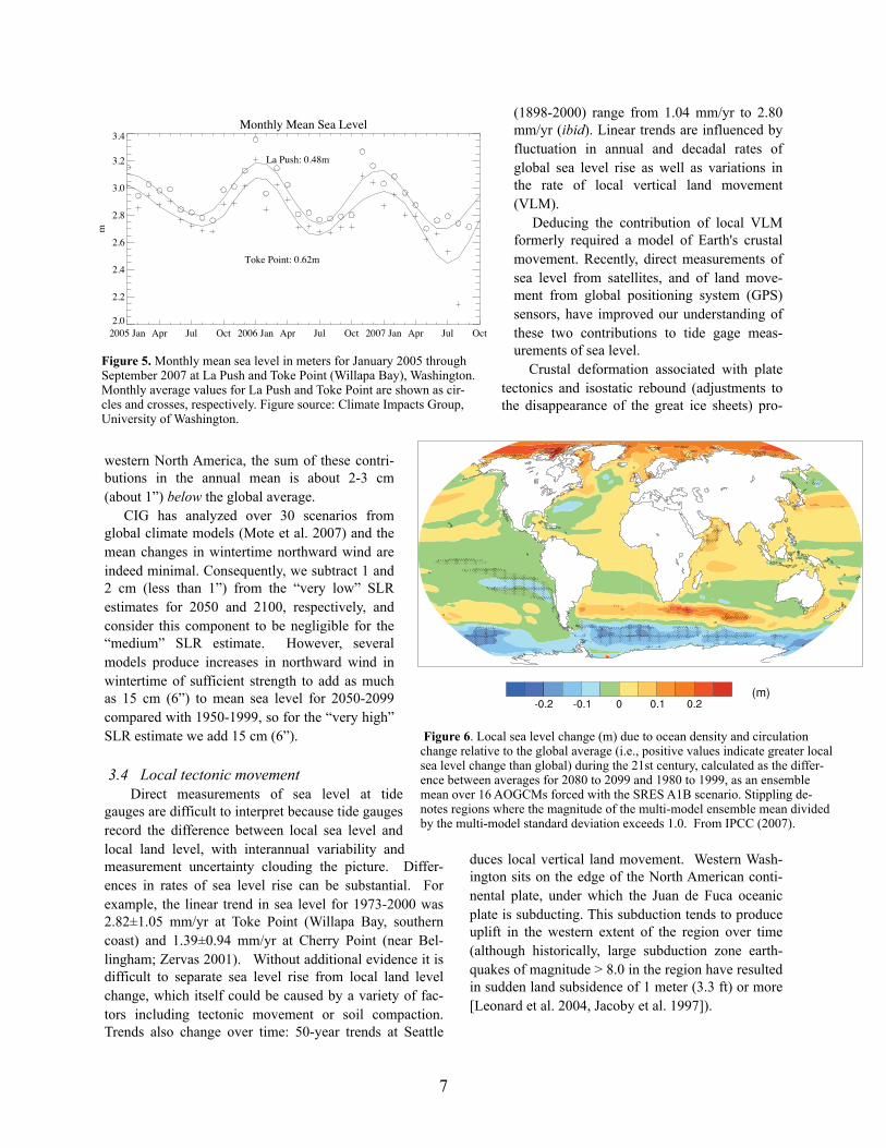
Figure 5. Monthly mean sea level in meters for January 2005 through September 2007 at La Push and Toke Point (Willapa Bay), Washington. Monthly average values for La Push and Toke Point are shown as cir-cles and crosses, respectively. Figure source: Climate Impacts Group, University of Washington.
An earlier analysis of records in the Pacific North-west (Holdahl et al. 1989) suggested that south Puget Sound was subsiding at a rate of approximately 2 mm/yr and the northwest Olympic Peninsula was rising at a comparable rate, while VLM on most of the Washington coast and the rest of Puget Sound was mostly less than 1 mm/yr. Another study by Mitchell et al. (1994) found little VLM in Puget Sound, but similar VLM for the coast as those of Holdahl et al. (1989).
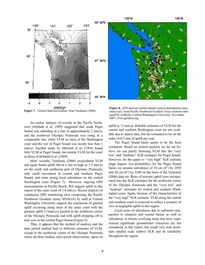
More recently, Verdonck (2006) recalculated VLM and again found uplift, but at a rate as high as 3.5 mm/yr on the north and northwest part of Olympic Peninsula, only small movement in central and southern Puget Sound, and some strong local subsidence on the central Washington coast (Figure 7). However, ongoing GPS measurements at Pacific Beach, WA suggest uplift in this region of the outer coast of 1.8 mm/yr. Recent analysis of continuous GPS monitoring sites comprising the Pacific Northwest Geodetic Array (PANGA) by staff at Central Washington University support the conclusion of general uplift occurring along most of the outer coast with the greatest uplift (>3mm/yr) located in the northwest corner of the Olympic Peninsula and with uplift dropping off to near zero in the central Puget Sound (Figure 8).
Thus, it appears that the method of analysis and the time period studied lead to different estimates of VLM, except in the northwest corner of the Olympic Peninsula where all three studies, and current observations, agree on
uplift at >2 mm/yr. Reliable estimates of VLM for the central and southern Washington coast are not avail-able due to sparse data, but are estimated to be on the order of 0-2 mm of uplift per year.
The Puget Sound basin seems to be the least consistent. Based on current analysis we do not be-lieve we can justify factoring VLM into the “very low” and “medium” SLR estimates for Puget Sound. However, for the upper or “very high” SLR estimate (high impact, low-probability) for the Puget Sound basin, we assume subsidence of 10 cm (4”) by 2050 and 20 cm (8”) by 2100 on the basis of the Verdonck (2006) data set. Rates of tectonic uplift were incorpo-rated into the SLR estimates for the northwest corner of the Olympic Peninsula and the “very low” and “medium” estimates for central and southern Wash-ington coast. Again, because of the characteristics of the “very high” SLR estimate, VLM along the central and southern coast is removed to reflect a scenario of zero or negligible uplift in this region.
Local areas of subsidence due to sediment com-paction in estuaries and coastal basins as well as subsidence in terrain overlying areas that have expe-rienced significant groundwater extraction are not considered in this report, but could very well domi-nate smaller scale relative SLR and its variability throughout the region.
8
Figure 7. Vertical land movements, from Verdonck (2006).Figure 8. GPS derived current annual vertical deformation rates (mm/year), from Pacific Northwest Geodetic Array (stations indi-cated by symbols), Central Washington University, November 2007, www.geodesy.org
4. Synthesis: Summary and calculation of SLR projections
Three important questions need to be considered in the use of SLR estimates in decision making:
1) what is the location of interest? 2) what time horizon should be considered?, and 3) what risk level is acceptable?
As indicated by Sections 3.3 and 3.4, location is important as rates of SLR vary depending on oceanographic condi-tions and on local VLM.
Time horizon is very important and will be defined by the nature of the decision being made; decisions with long life spans or long-term implications should be based on longer-term estimates of sea level rise. Note that time horizon is not just a function of the lifespan of a specific structure. The choice of time horizon should take into account the overall “footprint” of the decision, i.e., the committed long-term use of the site once it is developed.
For some factors that contribute to local SLR, changes will probably be linear with time so the 2050 value will be half the 2100 value. However, this is not the case for the most important term, global SLR: in most scenarios the rate of global SLR increases over time (the curve is concave upward or accelerating). Hence, it is inappropri-ate to estimate SLR in 2050 simply by halving an estimate of change that applies to the year 2100.
Finally, risk tolerance determines whether the medium or a less likely but higher (or lower) impact estimate is used. Risk tolerance will vary from community to com-munity, person to person, and project to project.
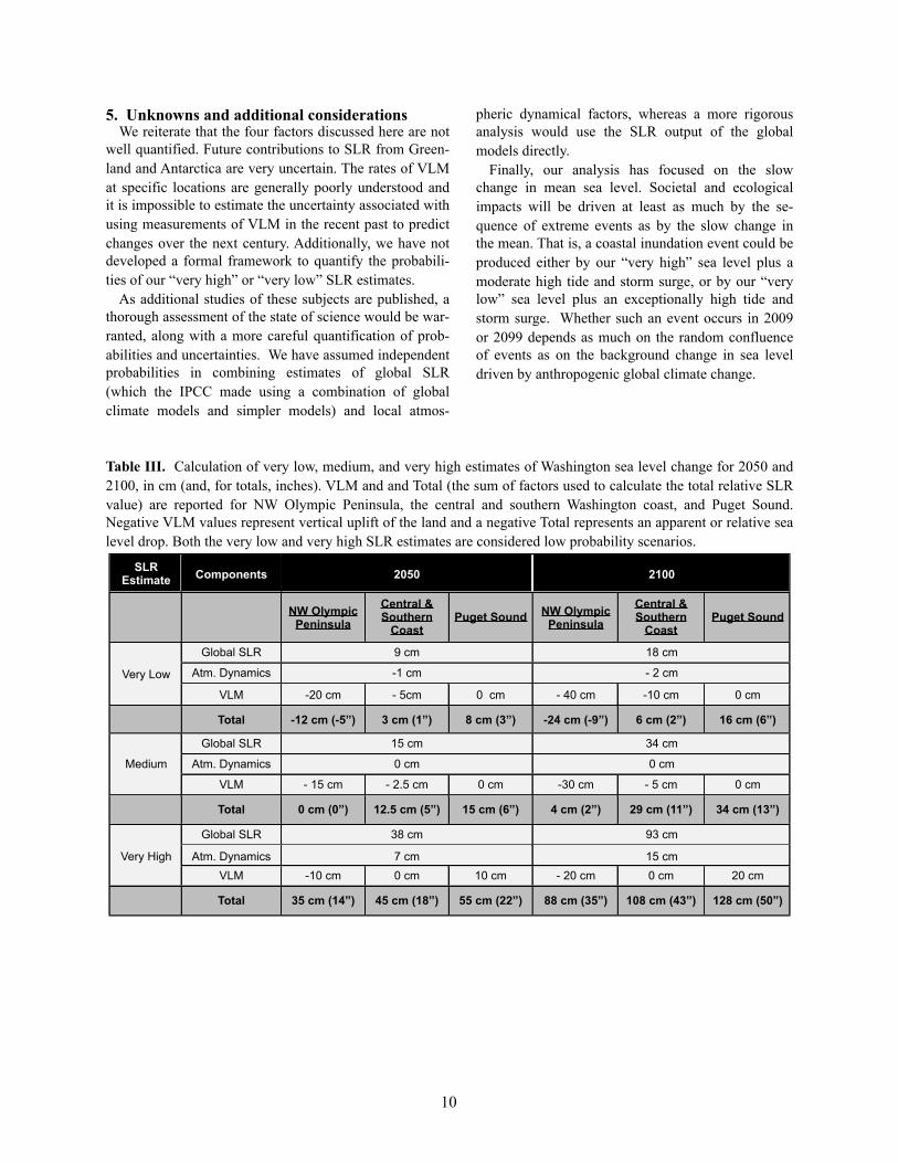
We now attempt to combine the factors in the above discussion to construct estimates of SLR for the NW Olympic Peninsula, the central and southern Washington coast, and Puget Sound for 2050 and 2100 (Table III). We stress that (1) these calculations have not formally quantified the probabilities, (2) SLR cannot be esti-mated accurately at specific locations, and (3) these numbers are for advisory purposes and are not actual predictions.
For the end-of-century “very low” SLR estimate, we use the 5% value of the B1 SLR scenario, namely 18 cm (7”) by 2100. The atmospheric component is assumed to be the same for all three areas and contributes –2 cm (less than –1”). For local contributions from VLM we take the low end of the various estimates discussed above: uplift in the NW Olympic Peninsula of 4 mm/yr (translates to a local SLR of –16” per century) and no uplift for Puget Sound. Uplift for the central and southern Washington coast is estimated at 1 mm/year (translates to a SLR of about –4” per century). Furthermore, global temperatures
in the B1 scenario level off by 2100. Consequently, the SLR profile is approximately linear (Figure 4), so the values in 2050 are half those in 2100.
For the end-of-century “medium” SLR estimate, we use the average of the six central values from the six IPCC scenarios (34 cm or 13”). The value for 2050 is somewhat below half of this value owing to the acceleration of SLR in all scenarios except B1 (Figure 4), with a low of 39% for A2 and a high of 50% for B1 and a mean of 45%. The atmospheric contribution is approximately zero. For the VLM term, we take the uplift value of 3mm/yr (translates to a SLR of –12” per century) for the NW Olympic Peninsula and 0.5 mm/yr (translates to a SLR of –2” per century) for the central and southern coast. For the Puget Sound basin, we again assume no change.
For the end-of-century “very high” SLR estimate, we start with the A1FI 95% value of 59 cm (23”) by 2100 but allow the possibility that the recent cryospheric contributions could continue and even increase in the 21st century. Although it is difficult to quantify the importance of such processes over the span of the 21st century, we take as a starting point the calculation in IPCC 2007 (Appendix 10.A.5). They presumed a linear relationship between global temperature anomalies (0.63°C) and enhanced ice sheet loss from these dynamical processes (0.32 mm/yr), and arrived at an estimate of 0-17 cm (0-7”) for the 21st century SLR. However, observations cannot constrain their estimate of 0.32 mm/yr within a factor of two. For example, one could posit a situation in which the difference between observed SLR and the sum of known terms during 1993-2003 (Table I) is entirely due to these processes; this gives an upper estimate of 1.3mm/yr, roughly a factor of 4 larger than their estimate. Likewise, there are small uncer-tainties in the estimated global temperature anomaly used in this ratio. Since an error of a factor of two in this ratio is plausible, we take that as a rough estimate of the upper limit of ice sheet contributions, adding 34 cm (13”) for 2100.
The atmospheric contribution in all areas is 15 cm (6”) by 2100 and 7 cm (3”) for 2050.
For the VLM term in our “very high” SLR esti-mate, we use an uplift value of 2 mm/yr (SLR about –8” per century) at the NW Olympic Peninsula. For the central and southern Washington coast, we as-sume zero VLM. For the Puget Sound region, subsi-dence of 2 mm/year (SLR about 8” per century) is used.
9
5. Unknowns and additional considerationsWe reiterate that the four factors discussed here are not
well quantified. Future contributions to SLR from Green-land and Antarctica are very uncertain. The rates of VLM at specific locations are generally poorly understood and it is impossible to estimate the uncertainty associated with using measurements of VLM in the recent past to predict changes over the next century. Additionally, we have not developed a formal framework to quantify the probabili-ties of our “very high” or “very low” SLR estimates.
As additional studies of these subjects are published, a thorough assessment of the state of science would be war-ranted, along with a more careful quantification of prob-abilities and uncertainties. We have assumed independent probabilities in combining estimates of global SLR (which the IPCC made using a combination of global climate models and simpler models) and local atmos-
pheric dynamical factors, whereas a more rigorous analysis would use the SLR output of the global models directly.
Finally, our analysis has focused on the slow change in mean sea level. Societal and ecological impacts will be driven at least as much by the se-quence of extreme events as by the slow change in the mean. That is, a coastal inundation event could be produced either by our “very high” sea level plus a moderate high tide and storm surge, or by our “very low” sea level plus an exceptionally high tide and storm surge. Whether such an event occurs in 2009 or 2099 depends as much on the random confluence of events as on the background change in sea level driven by anthropogenic global climate change.
Table III. Calculation of very low, medium, and very high estimates of Washington sea level change for 2050 and 2100, in cm (and, for totals, inches). VLM and and Total (the sum of factors used to calculate the total relative SLR value) are reported for NW Olympic Peninsula, the central and southern Washington coast, and Puget Sound. Negative VLM values represent vertical uplift of the land and a negative Total represents an apparent or relative sea level drop. Both the very low and very high SLR estimates are considered low probability scenarios.
SLR Estimate Components 2050 2100
NW Olympic Peninsula
Central & Southern
CoastPuget Sound NW Olympic
Peninsula
Central & Southern
CoastPuget Sound
Very Low
Global SLR 9 cm 18 cm
Atm. Dynamics -1 cm - 2 cm
VLM -20 cm - 5cm 0 cm - 40 cm -10 cm 0 cm
Total -12 cm (-5”) 3 cm (1”) 8 cm (3”) -24 cm (-9”) 6 cm (2”) 16 cm (6”)
Medium
Global SLR 15 cm 34 cm
Atm. Dynamics 0 cm 0 cm
VLM - 15 cm - 2.5 cm 0 cm -30 cm - 5 cm 0 cm
Total 0 cm (0”) 12.5 cm (5”) 15 cm (6”) 4 cm (2”) 29 cm (11”) 34 cm (13”)
Very High
Global SLR 38 cm 93 cm
Atm. Dynamics 7 cm 15 cmVLM -10 cm 0 cm 10 cm - 20 cm 0 cm 20 cm
Total 35 cm (14”) 45 cm (18”) 55 cm (22”) 88 cm (35”) 108 cm (43”) 128 cm (50”)
10
ReferencesChurch, J.A., and N.J. White, 2006: A 20th century ac-
celeration in global sea-level rise. Geophysical Research Letters 33, L01602, doi:10.1029/2005GL024826.
Holdahl, S.R., F. Faucher, and H. Dragert. 1989. Contempo-rary vertical crustal motion in the Pacific Northwest, in: Choen and Vanicek (eds), Slow deformation and transmis-sion of stress in the earth. American Geophysical Union, Geophysical Monograph 49.
Holgate, S.J., and P.L. Woodworth, 2004: Evidence for en-hanced coastal sea level rise during the 1990s. Geophysical Research Letters, 31, L07305, doi:10.1029/2004GL019626.
IPCC, 2007: Climate Change 2007: The Physical Science Basis. Contribution of Working Group I to the Fourth As-sessment Report of the Intergovernmental Panel on Climate Change [S. Solomon, D. Qin, M. Manning, Z. Chen, M. Marquis, K.B. Averyt, M. Tignor and H.L. Miller (eds.)]. Cambridge University Press, Cambridge, United Kingdom and New York, NY, USA.
(IPCC SPM) IPCC, 2007: Summary for Policymakers. In: Climate Change 2007: The Physical Science Basis. Contri-bution of Working Group I to the Fourth Assessment Report of the Intergovernmental Panel on Climate Change [Solo-mon, S., D. Qin, M. Manning, Z. Chen, M. Marquis, K.B. Averyt, M. Tignor and H.L. Miller (eds.)]. Cambridge Uni-versity Press, Cambridge, United Kingdom and New York, NY, USA.
Jacoby, G.C., D.E. Bunker, B.E. Benson, 1997: Tree-Ring evidence for an A.D. 1700 Cascadia earthquake in Wash-ington and northern Oregon. Geology 25(11): 999-1002
Leonard, L.J., R.D. Hyndman, S. Mazzotti, 2004: Coseismic subsidence in the 1700 great Cascadia earthquake: Coastal estimates versus elastic dislocation models. GSA Bulletin 116: 655-670, doi: 10.1130/ B25369.1
Leuliette, E.W., R.S. Nerem, and G.T. Mitchum, 2004: Cali-bration of TOPEX/Poseidon and Jason altimeter data to construct a continuous record of mean sea level change. Mar. Geodesy 27(1-2): 79-94.
Manizade, and C. Martin, 2006: Progressive increase in ice loss from Greenland. Geophysical Research Letters 33, L10503, doi: 10.1029/2006GL026075.
Mitchell, C.E., P. Vincent, R.J. Weldon II, and M.A. Richards, 1994: Present-day vertical deformation of the Cascadia margin, Pacific Northwest, United States. Journal of Geo-physical Research 99 (B6): 12257–12277.
Mote, P., E. Salathé, and E. Jump, 2007: Scenarios of future climate for the Pacific Northwest. A report prepared by the Climate Impacts Group (Center for Science in the Earth System, University of Washington, Seattle.)
Nerem, R., Leuliette, E., Cazenave, A., 2006: Present-day sea-level change: A review. C. R. Geoscience 338: 1077-1083.
Rahmstorf, S., 2007: A Semi-empirical approach to projecting future sea-level rise. Science. 315: 368-370.
Ruggiero, P., G.M. Kaminsky, G. Gelfenbaum, and B. Voigt, 2005: Seasonal to interannual morphodynamics along a high-energy- dissipative littoral cell. Journal of Coastal Research 21(3): 553-578. West Palm Beach (Florida), ISSN 0749-0208
Thomas, R., E. Frederick, W. Krabill, S. Manizade, and C. Martin, 2006: Progressive increase in ice loss from Green-land, Geophys. Res. Lett., 33, L10503, doi:10.1029/2006GL026075.
Velicogna, I., and J. Wahr, 2005: Greenland mass balance from GRACE. Geophysical Research Letters 32, L18505, doi:10.1029/2005GL023955.
Velicogna, I., and J. Wahr, 2006: Measurements of time vari-able gravity show mass loss in Antarctica. Science 311(5768): 1754–1756, doi:10.1126/ science.1123785.
Verdonck, D, 2006: Contemporary vertical crustal deforma-tion in Cascadia. Technophysics 417: 221–230.
Zervas, C, 2001: Sea Level Variations of the United States 1854-199. NOAA Technical Report NOS CO-OPS 36, National Oceanic and Atmospheric Administration, Na-tional Ocean Service, Center for Operational Oceano-graphic Products and Services, Silver Spring, MD.
Zwally, H.J., et al., 2006: Mass changes of the Greenland and Antarctic ice sheets and shelves and contributions to sea level rise: 1992-2002. Journal of Glaciology 51: 509–527.
11