Final Report of Senior Design Project Spring 2003

The University of California at Riverside Department of Electrical Engineering

Software Defined Radio Receiver

Prepared by: John Cortes, Varoon Malhotra Faculty Advisor: Yingbo Hua

Submitted on: June 9, 2003

2

Abstract:

The purpose of this project was to design a Software defined radio receiver for a

select set of signals. Software Radio has recently become a major investment area. It

offers portability, because software is much easier media to change than hardware. It is

also easier to design new modulation and demodulation schemes.

For the beginning of this project, research was done to see what kind of signals

could be easily captured, and to see if any could be affordably interfaced with existing

sound cards on computers. We propose the details for design of a cheap RF front end, and

some details on writing demodulation schemes in software for AM radio, NTSC, and FM

signals.

The result of this project produced an RF Front End that is portable and a set of

Matlab scripts for running various demodulation schemes that are portable to a vector

processing type computer. The one thing we did not accomplish was being able to

interface our Front End, for both AM and FM reception, to our computer through the

sound card due to difficulties in amplifying the signal with too much noise.

Keywords: AM, FM, Quadrature Demodulation, VCO, PLL, NTSC, Software Defined Radio, USB, LSB

3

Table of Contents: Page: Chapter One – Introduction 1.1 Introduction 4 1.2 Historical Perspective 5 1.3 Glossary of Acronyms and Abbreviations 6 Chapter Two - Design and Technical Results 2.1 Problem Statement 7 2.2 Design Specifications 7 2.3 Overall Goals 9 Chapter Three - Method of Solution 3.1 Introduction 10 3.2 AM Modulation 10 3.3 AM Receiver 12 3.4 Solution for AM receiver: 16 3.5 FM Front End and Quadrature Demodulator 18 3.6 R/C (Radio Control) Car Transmitters and Receivers 21 3.7 NTSC signal Demodulation 26

Chapter Four – Evaluation 4.1 Introduction 30 4.2 Discussion of Results/ Test Plan 30 4.3 Design Comparison / Design Trade Off 32 Chapter Five – Administrative 5.1 Introduction 33 5.2 Budget and/or Cost Analysis 33 Chapter Six – Elements of Design 6.1 The Final Product 34 Chapter Seven – Conclusion 7.1 Introduction 35 7.2 Expansion and Improvement 35 Acknowledgements 36 References 37 Appendix A: Parts List 38 Appendix B: Equipment List 39 Appendix C: Software List 40 Appendix D: Special Resources 59 Appendix E: Schematic Drawings 60 Appendix F: Pictures of Receiver and Quadrature Demodulator 64

4

Chapter One - Introduction 1.1 Introduction: Software defined radio reflects the convergence of two dynamically developing

technological forces of the 1990s – digital radio and software technology. The former

facilitated the wireless revolution that gave birth to the mobile phone mass market whilst

the latter, over the same period, has both facilitated the Internet wave. The massive

growth and convergence of these two markets is both enabling new applications on

second (2G) and third generation (3G) mobile communications networks and

simultaneously changing the preexisting ground rules of the wireless industry.

A software radio is a radio whose channel modulation waveforms are

defined in software. That is, waveforms are generated as sampled digital signals,

converted from digital to analog via a wideband DAC and then possibly upconverted

from IF to RF. The receiver, similarly, employs a wideband Analog to Digital Converter

(ADC) that captures all of the channels of the software radio node. The receiver then

extracts, down converts and demodulates the channel waveform using software on a

general purpose processor. Software radios employ a combination of techniques that

include multi-band antennas and RF conversion; wideband ADC and Digital to Analog

conversion (DAC); and the implementation of IF, baseband and bitstream processing

functions in general purpose programmable processors. The resulting software-defined

radio (or "software radio") in part extends the evolution of programmable hardware,

increasing flexibility via increased programmability. And in part it represents an ideal

that may never be fully implemented but that nevertheless simplifies and illuminates

tradeoffs in radio architectures that seek to balance standards compatibility, technology

insertion and the compelling economics of today's highly competitive marketplaces.

5

1.2 Historical Perspective

Originally a military and academic problem, SDR has now come to be notice as

the future of wireless communications. The idea of software patches for enabling phones

to operation in different environments and standards seems as the survival of the next

generation of phones.

The idea of a pure software radio is to connect the A/D converter as close to the

antenna as possible. The rest of the design is to design the software to work in emulation

of the effects of hardware, and at the end produce a usable baseband audio signal of

interest. This idea, at this moment, is unfeasible due to the frequency coverage of current

global telecommunications. The A/D converter would have to work up to a rate of a

Giga-samples/sec and beyond. This is not really feasible so therefore it becomes of

interest to design a front-end to this system: a hardware system that is able to select the

proper portion of the radio spectrum and down convert the signal, via superhetrodyne

techniques, to a more manageable frequency where it may be sampled and converted to

digital.

Figure 1: Pure Software Radio Concept

6

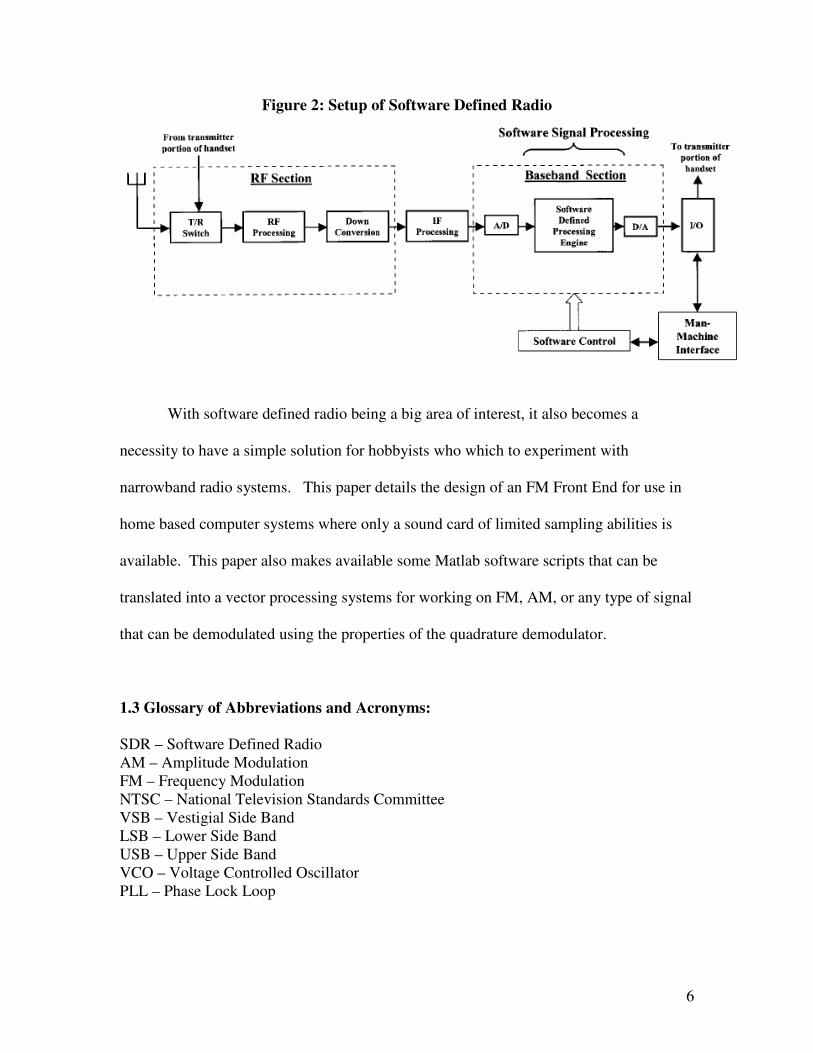
Figure 2: Setup of Software Defined Radio

With software defined radio being a big area of interest, it also becomes a

necessity to have a simple solution for hobbyists who which to experiment with

narrowband radio systems. This paper details the design of an FM Front End for use in

home based computer systems where only a sound card of limited sampling abilities is

available. This paper also makes available some Matlab software scripts that can be

translated into a vector processing systems for working on FM, AM, or any type of signal

that can be demodulated using the properties of the quadrature demodulator.

1.3 Glossary of Abbreviations and Acronyms: SDR – Software Defined Radio AM – Amplitude Modulation FM – Frequency Modulation NTSC – National Television Standards Committee VSB – Vestigial Side Band LSB – Lower Side Band USB – Upper Side Band VCO – Voltage Controlled Oscillator PLL – Phase Lock Loop

7

Chapter Two - Design and Technical Results:

2.1 Problem Statement

The goal of this project is to try and receive a radio signal by capturing that signal

through the sound card, then demodulating that signal in software, preferably in real time,

then output to the screen or audio the demodulated signal.

2.2 Design Specifications

For this project we are going to design a low cost solution for PC based hardware

radio. We will use an already common feature of computers to sample the signal: the

sound card. For this setup we will design the receiver system with hardware IF and

connect its output directly to one of the sound card’s input ports. From there we work on

the demodulation schemes for decoding Narrowband signals, preferably AM. If we get

these basics done quickly then we may continue to working on a tuner for FM signals,

and then work on a user interface for allowing of choosing a specific radio channel. If we

get everything working, then one of the final things we wish to accomplish is to be able

to decode regular NTSC TV signals.

Some of the framework for dealing with vector samples has been provided by the

GNU Radio project. This allows for a variety of software based demodulation schemes

to be conducted in any manner possible. The framework allows for the design of a

receiver. The project’s current work is being able to decode ATSC (Digital Television

signal) (edit: of which is now complete as of 6/2003).

8

The receiver will be designed to tune into specific frequencies and be able to

down convert the signal to an IF. From there we will sample the signal using the

soundcard of the computer system. Hopefully if everything is done correctly, the

sampled signal will be of good quality and will not have any aliasing in it; though it

seems that Narrowband signals are our only option right now.

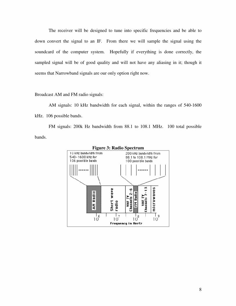
Broadcast AM and FM radio signals:

AM signals: 10 kHz bandwidth for each signal, within the ranges of 540-1600

kHz. 106 possible bands.

FM signals: 200k Hz bandwidth from 88.1 to 108.1 MHz. 100 total possible

bands.

Figure 3: Radio Spectrum

9

For the receiver and IF design, the design will be based on most of the work

developed by the American Radio Relay League (ARRL) society’s published material.

After the signal is sampled, depending on how fast the system performs, we will process

the signal using various DSP algorithms devised for demodulation of the signal. I/Q

channel separation, Digital IF, etc..., will all be emulated in software.

2.3 Overall Goals: The overall goal of this project is to have designed a working RF Front-End

system, this is reasonably low cost and not to difficult to build using off the shelf parts

and components easily orderable from Digi-Key and other IC providers. The system

design will allow it to be connected to any computer with reasonable audio capture

capabilities and design some software demodulation algorithms that will work for this

specific type of setup for working with AM and FM radio. We hope to contribute to the

some knowledge to the current workings of the GNU Software Defined Radio Project.

10

Chapter Three - Method of Solution:

3.1 Introduction:

The following set of materials describe the process of how we came up with the

AM Reciever, FM Front End, Quadrature Demodulator, and a description of the FM

transmitting system we purchased for testing our system. It also includes the information

on what we know about NTSC signals.

3.2 AM Modulation: The objective of modulation is to take a baseband signal that contains information

(voice, music, video, etc) and translate the signal to a new frequency so that it can be

transmitted easily and accurately over a communications channel. AM modulation is just

one of the different forms of modulation. AM has an output in which a carrier signal has

sideband energy generated by the modulation process added to or subtracted from the

carrier. The carrier is a steady unchanging signal and represents the middle of the

required communications channel. There is no information in the carrier, it is all in the

sideband signals. When one tunes in to a radio station the carrier frequency is the signal

you tune to.

If the baseband signal is m(t) then by multiplying this baseband signal by a cosine

wave at the carrier frequency the result is m(t) cos wct. This type of modulation shifts the

spectrum of m(t) to the carrier frequency. In this equation w is the frequency of the

modulating signal or baseband signal and wc is the carrier frequency.

m(t) cos (wct) <= > ½ [M(w + wc) + M(w-wc) ].

11

12

The upper sideband is (w+wc) and the lower sideband is (w-wc). Since AM has two

sidebands that are sopies of the original signal, the occupied bandwidth will be twice that

of the original signal. So for example if a baseband voice signal of about 3 kHz requires a

channel bandwidth of about 6 kHz.

3.3 AM Receiver:

To demodulate an AM signal you have to first downshift the signal to an

appropriate frequency. This is done by the process of mixing. Mixing is the same process

as Modulation for an AM signal. By multiplying the carrier with a local oscillator two

signals are produced; the sum and difference in frequency of the two inputs.

If the real carrier is y = cos(wot) and the local oscillator is cos(wt) when we mix these

two signals we get the product of the two inputs.

(cos wot) (cos wt) = [(e^jw0t + e^-jwot)/2] * [(e^jw0t + e^-jwot)/2]

= ¼ *[ [e^j(w + wo) + e^-j(w + wo)] + [e^j(wo-w)t + e^-j(wo-w)t] ]

= 1/2[ cos( wo + w)t + cos(wo-w)t]

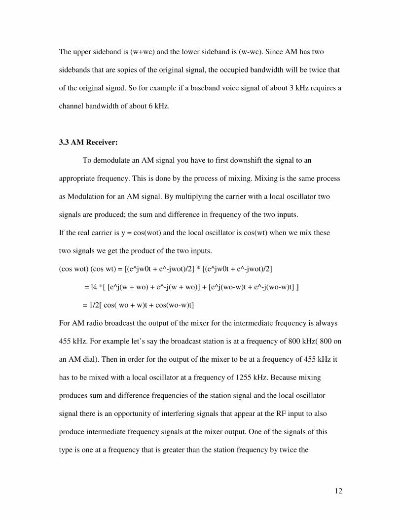
For AM radio broadcast the output of the mixer for the intermediate frequency is always

455 kHz. For example let’s say the broadcast station is at a frequency of 800 kHz( 800 on

an AM dial). Then in order for the output of the mixer to be at a frequency of 455 kHz it

has to be mixed with a local oscillator at a frequency of 1255 kHz. Because mixing

produces sum and difference frequencies of the station signal and the local oscillator

signal there is an opportunity of interfering signals that appear at the RF input to also

produce intermediate frequency signals at the mixer output. One of the signals of this

type is one at a frequency that is greater than the station frequency by twice the

13

intermediate frequency. These interfering signals are called image frequencies. So for

example if a station is at 600kHz and the local oscillator is changed to 1055 to tune in to

the station, then a station frequency at 1510 kHz is an image frequency because 1510-

1055 also produces an IF of 455 kHz. Image frequencies are produced at frequencies that

are twice the intermediate frequency away from the station frequency. One can reduce the

problems associated with image frequencies if you make sure that you decrease the

amplitude of the image frequencies before the mixer.

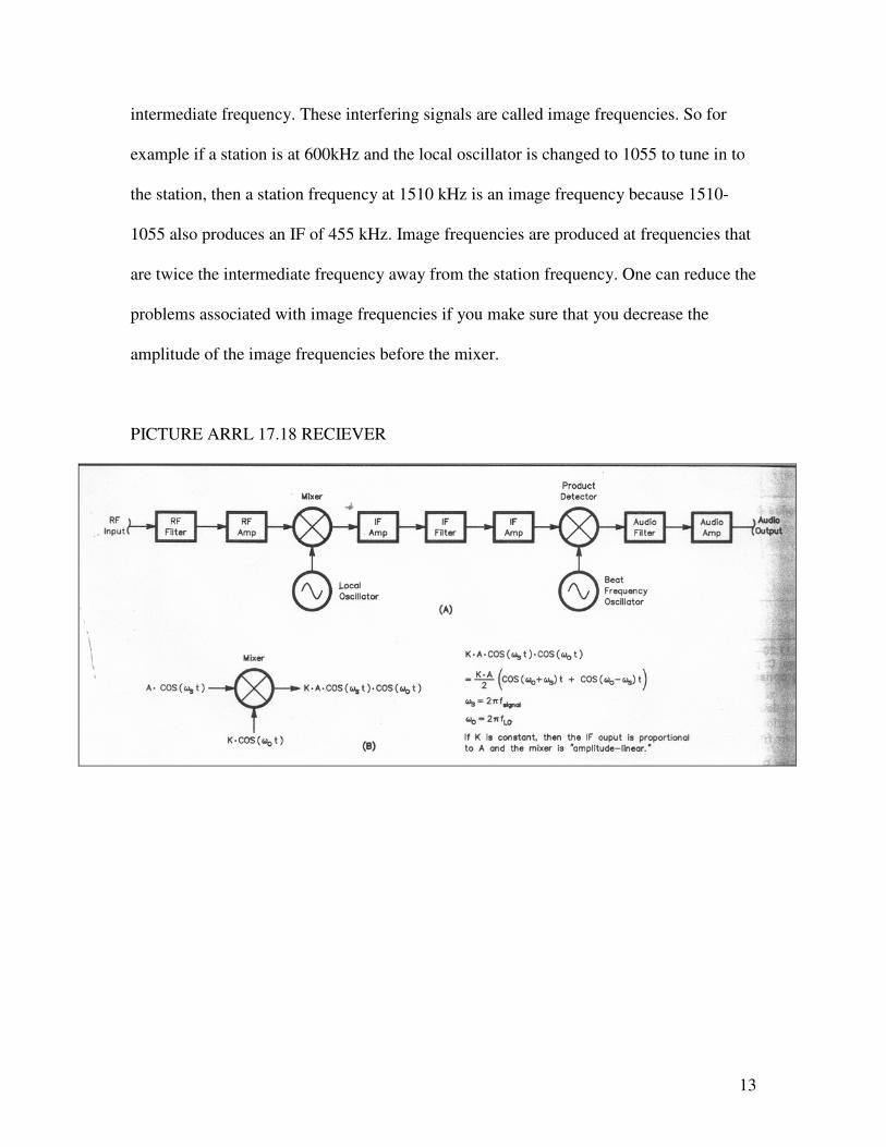
PICTURE ARRL 17.18 RECIEVER

14

The detector is used to demodulate the AM signal and produce the baseband signal from

the modulated signal. Detection translates the signal in the frequency spectrum back

down to the baseband frequency.

PICTURE ARRL AM DETECTION 15.8

15

3.4 Solution for AM receiver:

One of our goals was to be able to receive an AM signal and be able to

demodulate this signal using MATLAB. To demodulate an AM signal you have to take

the signal from the IF stage which is at 455 kHz. The problem was that we could not

demodulate the signal straight from the IF stage. An AM radio signal has a bandwidth of

10kHz so the total frequency range of the desired signal is from 450kHz – 460 kHz.

Therefore the maximum frequency present in the signal is 460 kHz. In order to

demodulate the signal directly one would need a 920 kHz sampler. This holds due to the

Nyquist criteria which states that in order to not lose information in a signal one must

sample the signal at a rate of twice the maximum frequency present in the signal. We are

using a soundcard as our A/D conversion unit and the soundcard works at 44.1 kHz. So in

order to not lose any information the signal that is sampled can’t be at a frequency higher

than 22.05 kHz.

We bought an AM receiver kit instead of building a receiver because we didn’t

want to run into the same problems that occurred with the FM receiver (for the RC car).

In order to not lose any information in the AM signal we had to first downshift the signal

at the IF (455 kHz) to about 15 kHz. Then we could easily use software demodulation

techniques in order to recover the baseband signal.

The problems occurred when we had to downshift the AM signal from the IF

frequency. In order to downshift the signal we used a voltage controlled oscillator and the

AM 455 kHz signal as inputs to a mixer.

16

It was very difficult to pick up any radio station due to the fact that the antenna

that the kit came with was poor. At most stations noise was all that was heard. The

voltage controlled oscillator was set to output a signal at 443 kHz. The VCO (voltage

controlled oscillator) was used as the low input for the mixer. The problem was that the

output of the mixer circuit would never be at the desired frequency. The output of the

mixer was just noise and no clean signal was seen when I analyzed this on the

oscilloscope. I added a low pass filter to the outputs of both the IF frequency and the

VCO to cancel unwanted signals. When viewed on the oscilloscope the output of the

VCO occurred in harmonics. In other words if there was a signal at 443 kHz then there

would also be a signal at 2*443kHz, 3*443kHz, etc. This is why we used a low pass filter

on the output of the VCO. The cutoff frequency for this filter was 443 kHz. We also used

a low pass filter for the output from the AM signal’s IF frequency. The cutoff frequency

for the filter was 460 kHz. The filters worked fine as was easy to see from the output on

the oscilloscope. The problem was that the voltage for both signals had to be the same for

the mixer to work correctly. If the voltages of both these signals differed by any amount

then the mixer would not function correctly.

The voltage level for the output of the VCO stayed at a fairly constant level of

approximately 1.4 volts, however the voltage at the output of the IF frequency fluctuated

drastically. Even if a clean signal was heard, the output fluctuated between a good signal

and noise very often. I believe that this fluctuation was ultimately the problem with the

circuit. The output voltage at the IF frequency was at times a few hundred millivolts and

at times was much higher. If the signal was looked at in the frequency domain on the

oscilloscope a clear peak was seen at 455 kHz but in the time domain the peak to peak

17

voltage amplitude was very unstable. We added an op-amp to amplify the output at the IF

frequency but this ultimately did not improve the situation. I believe that equipment was

the flaw in this aspect of the design. The AM receiver kit was not very good and that’s

why it was hard to pickup a good signal. It might have been possible to find another

mixer which outputs the difference of both frequencies even if the power is different in

both signals, but I’m not sure about this. More time was spent designing the FM receiver

for the RC car so maybe if there was more time better equipment could be bought for an

AM receiver. More knowledge of RF hardware design also would have helped in this part

of the design.

3.5 FM Front End and Quadrature Demodulator:

When we started out this project we found out from many papers that quadrature

demodulation was the best thing to go with. If a system has 2 lines for input, say like a

stereo line input for a computer, then quadrature demodulation will offer twice the

normal bandwidth of just a normal single channel system. In Gerald Youngblood’s

article, “A Software-Defined Radio for the Masses”, his system used a system similar to

the quadrature demodulator and had been demonstrated to work ok with a good sound

card sampler. Using his general layout of the system we decided to base our front end

system on it.

18

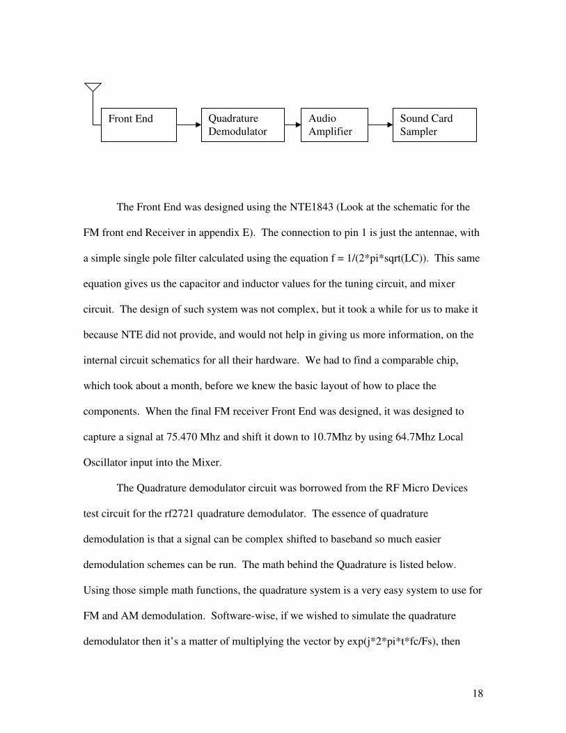
The Front End was designed using the NTE1843 (Look at the schematic for the

FM front end Receiver in appendix E). The connection to pin 1 is just the antennae, with

a simple single pole filter calculated using the equation f = 1/(2*pi*sqrt(LC)). This same

equation gives us the capacitor and inductor values for the tuning circuit, and mixer

circuit. The design of such system was not complex, but it took a while for us to make it

because NTE did not provide, and would not help in giving us more information, on the

internal circuit schematics for all their hardware. We had to find a comparable chip,

which took about a month, before we knew the basic layout of how to place the

components. When the final FM receiver Front End was designed, it was designed to

capture a signal at 75.470 Mhz and shift it down to 10.7Mhz by using 64.7Mhz Local

Oscillator input into the Mixer.

The Quadrature demodulator circuit was borrowed from the RF Micro Devices

test circuit for the rf2721 quadrature demodulator. The essence of quadrature

demodulation is that a signal can be complex shifted to baseband so much easier

demodulation schemes can be run. The math behind the Quadrature is listed below.

Using those simple math functions, the quadrature system is a very easy system to use for

FM and AM demodulation. Software-wise, if we wished to simulate the quadrature

demodulator then it’s a matter of multiplying the vector by exp(j*2*pi*t*fc/Fs), then

Front End Quadrature Demodulator

Audio Amplifier

Sound Card Sampler

19

running a simple FIR low-pass filter. A feat not to hard in software especially in

MATLAB.

Table 3.1: The math of Quadrature Demodulation

��������� ����

�������

���������� �

��

��

�� ��������

�� ��������

������ ���� ����

)()(

)())2sin()2)(cos((

))((/))(/)(arctan()(

)()(

)2sin()()()2cos()()(

2

2

22

fofXetx

etxftjfttx

tdtdFM

tItQt

tQtIAM

fttxtQ

fttxtI

ftj

ftj

−==+

Θ==Θ

+=

==

π

πππ

ππ

20

For the audio amplifier part of the circuit, we used low noise audio amplifier that we

purchased from Digi-Key, the LT1115 IC’s. The circuits were pretty self explanatory.

We used electrolyte capacitors to filter out the DC power, and we used a low pass non-

inverting setup, with frequency cutoff around 30Khz.

3.6 R/C (Radio Control) Car Transmitters and Receivers:

Since I was already using a pre-made FM transmitter, we had to learn as much as

we could about the specifications about how the FM transmitter was designed and how it

functions. I purchased an R/C transmitter and receiver system from Tower Hobbies, the

Hitec Ranger III FM 3 channel Transmitter and Receiver.

21

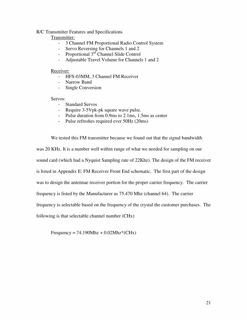
R/C Transmitter Features and Specifications Transmitter:

- 3 Channel FM Proportional Radio Control System - Servo Reversing for Channels 1 and 2 - Proportional 3rd Channel Slide Control - Adjustable Travel Volume for Channels 1 and 2

Receiver: - HFS-03MM, 3 Channel FM Receiver - Narrow Band - Single Conversion

Servos:

- Standard Servos - Require 3-5Vpk-pk square wave pulse. - Pulse duration from 0.9ms to 2.1ms, 1.5ms as center - Pulse refreshes required ever 50Hz (20ms)

We tested this FM transmitter because we found out that the signal bandwidth

was 20 KHz. It is a number well within range of what we needed for sampling on our

sound card (which had a Nyquist Sampling rate of 22Khz). The design of the FM receiver

is listed in Appendix E: FM Receiver Front End schematic. The first part of the design

was to design the antennae receiver portion for the proper carrier frequency. The carrier

frequency is listed by the Manufacturer as 75.470 Mhz (channel 64). The carrier

frequency is selectable based on the frequency of the crystal the customer purchases. The

following is that selectable channel number (CHx)

Frequency = 74.190Mhz + 0.02Mhz*(CHx)

22

R/C Transmitter Specs: From Data Acquisition to FM Modulation and

Transmission

Analog Pot. Control Stick 0 – 5V range, centered at 2.5V

Read 3 channels into Microcontroller using A/D and compare to 2.5V in software (2.5 V considered as center = 1.5ms pulse width)

Allot 0.9 to 2.1ms of pulse time to each channel on the 20ms stream

FM modulate signal around a center frequency, 10.7Mhz

Shift spectra to a specified frequency chosen by the manufacturer’s crystal set (79.470Mhz)

2.0 ms = 5.0 V 1.5 ms = 2.5 V 1.0 ms = 0.0 V PW = 1.5*voltage + 1ms

Pulse Stream output reading channels sequentially and leaving empty space until 50Hz synchronization

Hardware Software/ MicroController

23

R/C Receiver Specs: From Reception to Final Output

Receive Signal at 79.470 Mhz, and Shift Down to 10.7Mhz

Hardware Software/ Microcontroller

FM Demodulate Signal at 10.7Mhz

Amplify Signal into a sharp Square Wave using a Voltage Comparator to convert into 50Hz 5Vpk-pk

Synchronize signal to 50Hz and do Input Capture on rising edges

Channel 1 = 1st edge Channel 2 = 2nd edge Channel 3 = 3rd edge Sync to 20ms

Output each Channel to difference Output ports on microcontroller

Each output port is fed into individual servos

24

Pulse Width Information:

Figure X: Servo Signals and FM Receiver Signals for Positive and Negative Shift Modulation

Positive Shift Modulation: Approximately 1ms to 2ms total pulse with time so therefore 0.5us dedicated up Pulse time, with rest of time filled in as 0. Negative Shift Modulation: Vice versa of Positive Shift Modulation. In order to decode this in software, the properties of the microcontroller must be

able to sync to the 50Hz signal from the r/c car transmitter. In Matlab it’s a matter of

being able to count the proper number of steps in the signal given the proper sampling

rate. Since most of the hardware was not working until near the end of the quarter, we

decided to simulate the pulse stream by reading the output directly into the HC11 then

mixing the signals and sending the final output stream to MATLAB. Appendix C lists

Servo 1

Servo 2

Servo 3

Pulse Train +Shift Modulation

Pulse Train -Shift Modulation

25

the PulseStream.h and PulseStream.cpp files that were generated to work with the Analog

outputs of the HC11 and simulate the FM transmitter, before modulation, and then the

output is applied to the sound card. Beyond that, since we were near the end, we decided

not to demodulate the pulse stream and therefore decided to dedicate more of our time

towards demodulation of the NTSC signal.

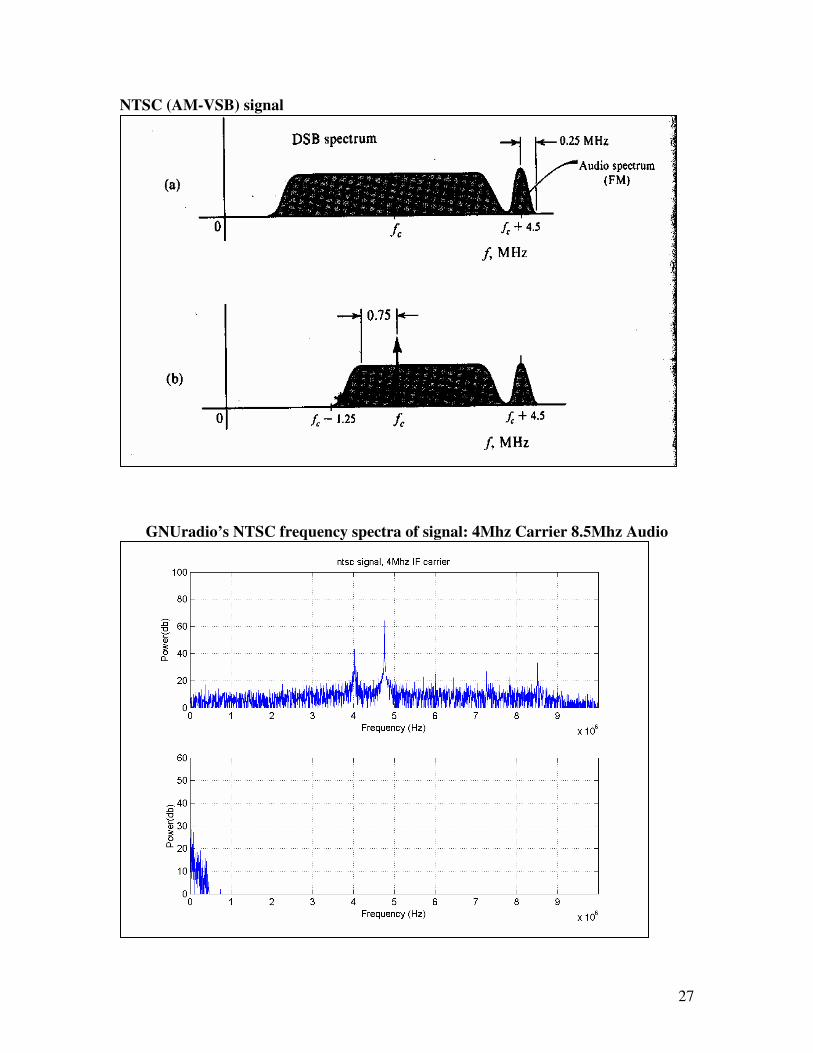
3.7 NTSC signal Demodulation:

NTSC is a special type of AM modulation that cuts of a portion of the lower

sideband, aka vestigial sideband modulation, and then attaches a carrier frequency to the

signal and an fm audio signal signal at 4.5MHz + carrier frequency. The demodulated

signal consists of a monochrome signal plus a quadrature modulated color component.

For our system we worked directly in software, and our NTSC data was provided from

the gnuradio’s leader: Eric Blossom.

NTSC Information: 525 Lines, VBI after 525/2 Lines 525 elements per line Interlaced frames at 60Hz 1 picture transmitted at 30Hz Bandwidth of 4.1Mhz essential information In order to demodulate the signal, first a quadrature demodulator is run at the

4Mhz carrier frequency. The signal is then processed through a Low Pass filter of

0.5Mhz, so only the monochrome (grayscale image stays). The final signal is then passed

through a syncing detector that first detects the VBI (Vertical Blanking Interval) then

starts capturing the Horizontal information on each of the horizontal peaks. The

grayscale information is mapped from one horizontal peak to the next. The Matlab code

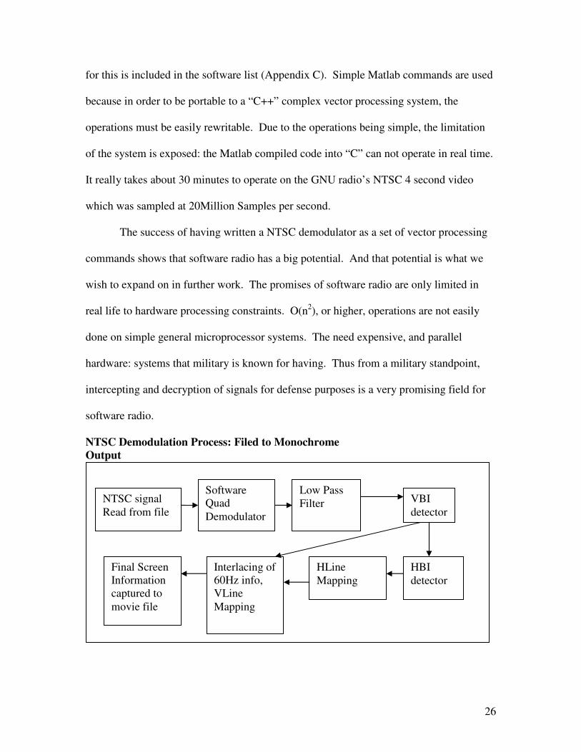
26

for this is included in the software list (Appendix C). Simple Matlab commands are used

because in order to be portable to a “C++” complex vector processing system, the

operations must be easily rewritable. Due to the operations being simple, the limitation

of the system is exposed: the Matlab compiled code into “C” can not operate in real time.

It really takes about 30 minutes to operate on the GNU radio’s NTSC 4 second video

which was sampled at 20Million Samples per second.

The success of having written a NTSC demodulator as a set of vector processing

commands shows that software radio has a big potential. And that potential is what we

wish to expand on in further work. The promises of software radio are only limited in

real life to hardware processing constraints. O(n2), or higher, operations are not easily

done on simple general microprocessor systems. The need expensive, and parallel

hardware: systems that military is known for having. Thus from a military standpoint,

intercepting and decryption of signals for defense purposes is a very promising field for

software radio.

NTSC Demodulation Process: Filed to Monochrome Output

NTSC signal Read from file

Software Quad Demodulator

Low Pass Filter VBI

detector

HBI detector

HLine Mapping

Interlacing of 60Hz info, VLine Mapping

Final Screen Information captured to movie file

27

NTSC (AM-VSB) signal

GNUradio’s NTSC frequency spectra of signal: 4Mhz Carrier 8.5Mhz Audio

28

NTSC demodulated signal : Horizontal & Vertical Syncing information

Demodulated NTSC time domain signal: Peaks represent Horizontal Syncs

29

Chapter Four – Evaluation

4.1 Introduction

We wanted to rest each part individually and see how the operate as a functioning

unit. If the meet the specs then all parts were to be combined, and interfaced. We had

three functioning units to test: the FM receiver, the Quadrature Demodulator, the

interface to the computer through the computer’s sound card.

4.2 Discussion of Results/ Test Plan

The hardware quadrature demodulate was a fine piece of material. To test it we

applied to signals, both of some frequency difference so that we would expect the

frequency mixing to work. When mixing two cosine signals, the expected output has

signal peaks at the sum and difference of the frequencies. Example: if we mix a signal of

75Mhz with a signal of 65MHz, the expected output should have a signal with peak

centered at 10Mhz( 75Mhz -65Mhz) and 140Mhz( 75Mhz + 65Mhz).

The rated specs of the quadrature list that a Local Oscillator x 2 must be applied

to the LO input of the rf2721 input; the chip divides the Local Oscillator frequency by

two so that it doesn’t leak into the output. The rated specs of the chip state that the inputs

must have a 100mv pk-pk input for both the low and the RF-IF. We tested the circuit

giving multiple range of frequencies, and the output matched what we expected when

mixing two signals of equal strength. The quadrature proved itself to work just fine, and

assuming we gave it the proper mixing frequency, the expected output would be correct.

For our computer system, we had to if each of the lines gave a descent input with

the sound card. To test it we decided to use the Matlab Data Acquisition Toolbox and

30

run the fft_demoai.m file to see the FFT spectra of the signal along with the real time

signal. One thing we discovered near the end was that the sound card, even though we

selected to input on 2 lines, the system was of low quality that the Left Channel leaked

into the Right channel, and vice versa for the Right Channel. Due to this problem we

decided to forgo using the hardware PCB quadrature demodulator because we would

never get a 2 channel system working, therefore we wrote the quadrature demodulate in

the software, which is only about 2 lines of Matlab code.

The FM Receiver had to receiver a power signal at 75.470Mhz and then had to

shift the signal to 10.7Mhz. Even though no images of the shifted output are included,

the NTE1843 did its job; all we had to do was supply the proper biasing voltage and

shunting capacitors, plus the LC values for each of the tuning and mixing circuits.

Since our Quadrature Demodulator didn’t work, we decided to instead use and

NTE1103 mixing circuit for mixing the signal down to near DC values; a frequency

where the sound card could pick it up. We didn’t use the quadrature demodulator single

I(t) output to the sound card because when we tried amplifying the output, the amplifiers

gave a lot of noise. We spent most of the second quarter trying to debug how to lower

the noise, but it came to no avail. We next tried the NTE1103 because it had a better

noise resilience, but in the end it ended up acting terribly because the amplification our

sound card required was well beyond 100x and the amplifier setup we designed couldn’t

accept a gain of that much and expect to fight noise in the same time.

One problem of why we couldn’t interface our FM receiver, then mix the signal

down to near-DC frequencies was that the noise of the system increased exponentially as

we came closer to DC, especially at 11.05Khz. One type of noise is listed as the 1/f

31

noise, ie: noise increases as you decreased the frequency. The same thing happened

when we tried mixing the AM signal of 455Khz to 11.05Khz, there was just too much

noise. Noise was our major problem, and if we could have gotten the noise suppressed

and a descent amplifier with large gain built, I believe we could have accomplished our

goals of this project for designing a narrowband FM and AM receiver.

On the software side, the scripts are provided and were tested using the GNU

radio’s library of sampled data. The had a couple of examples of FM modulated signals,

and one NTSC signal, along with an ATSC (hdtv) signal. The software portion of the

project worked just fine if we applied normalization to the signal.

4.3 Design Comparison/ Design Trade Off

What we did manage to complete was a set of Matlab scripts which were able to

read from a specific file and then demodulate the output using the software version of

quadrature demodulation. The output could then be AM demodulated, (gain of the

complex baseband signal) or FM demodulated (derivate of the phase of the signal, simple

FM demodulator shown on the Software Attachement: process_file.m). Since we had a

working AM demodulator, we designed a simple NTSC demodulator; the code is

provided.

32

Chapter Five – Administrative

5.1 Introduction

For this project we didn’t really want to spend a lot of money on hardware. One

of our initial specs was to work as little as possible on hardware, and write as much as

possible on software. In the end it didn’t turn out that way.

5.2 Budget and Cost Analysis:

We set up our budget at around $100. It was a reasonable sum to work from.

Each of the chips we purchased was around $5 each. We purchased most of the

capacitors from Electronics Warehouse for about $6. The resistors, we found available in

the EE communications lab cabinet for free. The RF2721 Quadrature demodulator we

got for free at RFmicro Devices (rfmicro.com). The TI CD74HC7046A VCO we got for

free at www.ti.com. The total parts price came out to $57, for the FM front end and

Quadrature Demodulator circuits. It was well within our rules for designing our FM

Front End.

Near the end of our project we couldn’t get the FM interfacing to work so we

decided to purchase an AM receiver circuit and use the 455Khz IF output. The kit cost

$35.

The final parts list came out to $97.

33

Chapter Six – Elements of Design

6.1 The Final Product

The outcome of this project produced a working FM receiver for any frequency

band that can be tuned down to 10.7 Mhz. The working system can, for aesthetic

qualities, be miniaturized to co-exist with the quadrature demodulator as a single chip

system powered by a 9v battery supply.

The only problem with SDR, on the ethics front, is that it if a transceiver design is

produced then any frequency band of choice is open for transmission and thus will cause

problems with the FCC. It would be advisable for the user of the system to consider

getting a ham license for operator of such equipment, for the right to transmit on the ham

frequencies.

The social impacts of this product are not easily identifiable, though the Software

Defined Radio concept has been creeping up in years and is demonstrated today on the

cellular networks, a very important part of many people’s lives. As for other design

factors, since the final product could not be completed, and the working model was

designed to work on a select set of frequencies there were no other easily identifiable

safety and economic factors.

34

Chapter Seven – Conclusion

7.1 Introduction:

In the area of SDR, there is no complete set of tools that can be easily design. A

working system must be specific on what type of signals the user is willing to decode,

and what range of frequencies the user wishes to work on. In our case we wanted to

decode a FM and AM narrowband signals,

We tried interfacing the outputs from the receiver circuits, but interfacing these

signals to our sound card could not be completed because of too much noise. Since we

wanted to demonstrate the functionality of SDR we chose to decode an NTSC raw signal.

Decoding of the signal was accomplished, at least for the monochrome signal. The

success of this proved to us, that SDR is a very good field of work which has lots of

potential because of it’s feasibility and portable setup.

7.2 Expansion and Improvement:

An idea for improvement of this project would be in the future to totally bypass

most of the capturing on the computer. A separate RF Front End programmable module

that sends a quadrature demodulated signal down a USB2 or IEEE1394 port. One would

need to look at special DSP chips and build the surrounding circuitry, which in itself is

another senior design project.

35

Acknowledgements

Thanks to Dr. Yingbo Hua for helping guide us on our project. Thanks to the EE175 professors for making this a wonderful course. Thanks to Dan Giles for helping us on the Cadence set of programs, and for producing our quadrature demodulator PCB, and also finally for being just a technical reference for most of us. Thanks to Eric Blossom for making the radio samples available online at www.comsec.com, especially the NTSC signal. Without those samples, it would have been impossible to write up any code to test our hypothesis.

36

References [1] Read, Dana G. The ARRL Handbook For Radio Communications, CT: The American Radio Relay League, 2003. [2] Jesme, Ron, Micro R/C Receiver, 3M Company. [3] Bowick, Chris. RF Circuit Design, MA: Elsevier Science, 1997. [4] B.P. Lathi, Modern Digital and Analog Communications Systems, New York, Oxford University Press, 1998. [5] D. Pulley, B. Rupert, “A Total Cost Approach to Evaluating Different Reconfigurable Architectures for Baseband Processing in Wireless Receivers,” IEEE Communications Magazine, Vol. 41, No. 1, pp. 105-113, 2003. [6] Tuttlebee, Walter. Software Defined Radio, John Wiley & Sons, Ltd. 2002, ISBNs: 0-470-84318-7 (Hardback); 0-470-84600-3 (Electronic). [7] Tuttlebee, Walter. Software Defined Radio: Origins, Drivers and International Perspectives. John Wiley & Sons, Ltd. 2002 ISBNs: 0-470-84464-7 (Hardback); 0-470-84601-1 (Electronic). [8] G. Youngblood, “A Software-Defined Radio for the Masses, Part 1”, QEX magazine, American Radio Relay League, July/August 2002

37

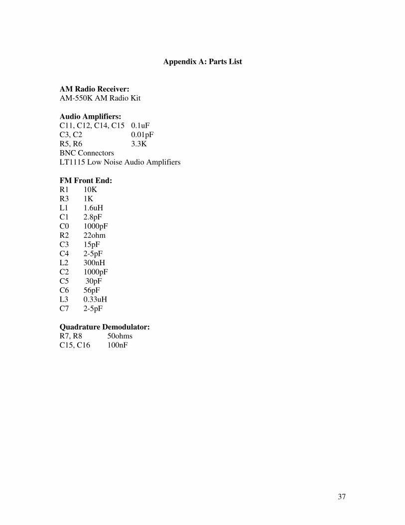
Appendix A: Parts List

AM Radio Receiver: AM-550K AM Radio Kit Audio Amplifiers: C11, C12, C14, C15 0.1uF C3, C2 0.01pF R5, R6 3.3K BNC Connectors LT1115 Low Noise Audio Amplifiers FM Front End: R1 10K R3 1K L1 1.6uH C1 2.8pF C0 1000pF R2 22ohm C3 15pF C4 2-5pF L2 300nH C2 1000pF C5 30pF C6 56pF L3 0.33uH C7 2-5pF Quadrature Demodulator: R7, R8 50ohms C15, C16 100nF

38

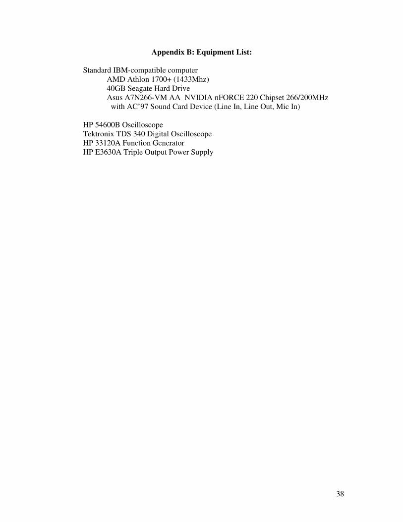
Appendix B: Equipment List: Standard IBM-compatible computer AMD Athlon 1700+ (1433Mhz) 40GB Seagate Hard Drive Asus A7N266-VM AA NVIDIA nFORCE 220 Chipset 266/200MHz with AC’97 Sound Card Device (Line In, Line Out, Mic In) HP 54600B Oscilloscope Tektronix TDS 340 Digital Oscilloscope HP 33120A Function Generator HP E3630A Triple Output Power Supply

39

Appendix C: Software List Matlab v6 GNU c++ compiler Cadence Pspice

40

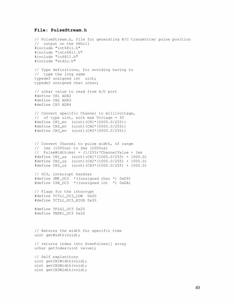
File: PulseStream.h // PulseStream.h, file for generating R/C transmitter pulse position // output on the 68hc11 #include "int6811.h" #include "intr6811.h" #include "io6811.h" #include "stdio.h" // Type definitions, for avoiding having to // type the long name typedef unsigned int uint; typedef unsigned char uchar; // uchar value to read from A/D port #define CH1 ADR2 #define CH2 ADR3 #define CH3 ADR4 // Convert specific Channel to millivoltage, // of type uint, with max Voltage = 5V #define CH1_mv (uint)(CH1*(5000.0/255)) #define CH2_mv (uint)(CH2*(5000.0/255)) #define CH3_mv (uint)(CH3*(5000.0/255)) // Convert Channel to pulse width, of range // 1ms (1000us) to 2ms (2000us) // PulseWidth(ms) = (1/255)*ChannelValue + 1ms #define CH1_us (uint)(CH1*(1000.0/255) + 1000.0) #define CH2_us (uint)(CH2*(1000.0/255) + 1000.0) #define CH3_us (uint)(CH3*(1000.0/255) + 1000.0) // OC3, interrupt handler #define JMP_OC3 *((unsigned char *) 0xD9) #define ISR_OC3 *((unsigned int *) 0xDA) // Flags for the interrupt #define TCTL1_OC3_LOW 0x20 #define TCTL1_OC3_HIGH 0x30 #define TFLG1_OC3 0x20 #define TMSK1_OC3 0x20 // Returns the width for specific time uint getWidth(void); // returns index into DownPulses[] array uchar getIndex(uint value); // Self explanitory uint getCH1Width(void); uint getCH2Width(void); uint getCH3Width(void);

41

// Array of Pulse times, converse to 0.5us up Pulse const uint DownPulses[] = { 1000,1200,1400,1600,1800, 2000,2200,2400,2600,2800, 3000 }; // Constant Up Pulse Time const uint UpPulse = 1000; // Total Pulse time that can be taken by multiplexing the // signals, 20ms(50Hz) = 40000 Pulses at 5e-7seconds const uint TotalPulseWidth = 40000; // Temp variables for counting uint current_cnt = 0; uint taken_width = 0; // Pulse Width time are stored into these values // only being read in the while(1) of main(void) uint CH1_width = 0; uint CH2_width = 0; uint CH3_width = 0;

42

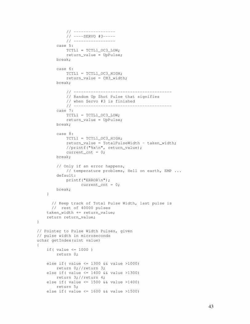
File: PulseStream.cpp #include "pulseStream.h" // Interrupt handler for OC3 to output // multiplex Pulse Stream :) interrupt void oc3_handler(void) { TFLG1 |= TFLG1_OC3; TOC3 = TCNT + getWidth(); } // Returns Pulse Width for current status of // Multiplexing uint getWidth(void) { uint return_value =0; current_cnt++; // Stream is as follows: // 1 2 3 4 5 6 7 8 20ms // ___ ___ ___ ___ // __| |___| |___| |___| |______________| switch(current_cnt) { // ----------------- // ----SERVO #1----- // ----------------- // Current spot is #1, generate 0.5us Up Pulse case 1: taken_width = 0; TCTL1 = TCTL1_OC3_LOW; return_value = UpPulse; break; // #2, Generate Rest of Pulse Time = PulseTime - 0.5us, // but read from table directly case 2: TCTL1 = TCTL1_OC3_HIGH; return_value = CH1_width; break; // ----------------- // ----SERVO #2----- // ----------------- case 3: TCTL1 = TCTL1_OC3_LOW; return_value = UpPulse; break; case 4: TCTL1 = TCTL1_OC3_HIGH; return_value = CH2_width; break;

43

// ----------------- // ----SERVO #3----- // ----------------- case 5: TCTL1 = TCTL1_OC3_LOW; return_value = UpPulse; break; case 6: TCTL1 = TCTL1_OC3_HIGH; return_value = CH3_width; break; // ---------------------------------------- // Random Up Shot Pulse that signifies // when Servo #3 is finished // ---------------------------------------- case 7: TCTL1 = TCTL1_OC3_LOW; return_value = UpPulse; break; case 8: TCTL1 = TCTL1_OC3_HIGH; return_value = TotalPulseWidth - taken_width; //printf("%x\n", return_value); current_cnt = 0; break; // Only if an error happens, // temperature problems, Hell on earth, EMP ... default: printf("ERROR\n"); current_cnt = 0; break; } // Keep track of Total Pulse Width, last pulse is // rest of 40000 pulses taken_width += return_value; return return_value; } // Pointer to Pulse Width Pulses, given // pulse width in microseconds uchar getIndex(uint value) { if( value <= 1000 ) return 0; else if( value <= 1300 && value >1000) return 0;//return 3; else if( value <= 1400 && value >1300) return 3;//return 4; else if( value <= 1500 && value >1400) return 5; else if( value <= 1600 && value >1500)

44

return 7;////return 6; else if( value <= 2000 && value >1600) return 10;//return 7; return 0; // This part intentionally commented out // so that Searching time is much smaller, // but proportionally it works just fine, // unless the ATV is readjusted, // Croc hunter's voice: "bad...bad...bad" /* else if( value <= 1100 && value >1000 ) return 1; else if( value <= 1200 && value >1100) return 2; else if( value <= 1300 && value >1200) return 0;//return 3; else if( value <= 1400 && value >1300) return 3;//return 4; else if( value <= 1500 && value >1400) return 5; else if( value <= 1600 && value >1500) return 7;////return 6; else if( value <= 1700 && value >1600) return 10;//return 7; else if( value <= 1800 && value >1700) return 8; else if( value <= 1900 && value >1800) return 9; else if( value <= 2000 && value >1900) return 10; return 0; */ } // Just a random wait time void wait(void) { uint i=0; for(i=0; i<40000; i++); } // Initializations void init(void) { // Set OC3 interrupt flag TMSK1 = 0x20; // Clear oc3 flag

45

TFLG1 |= 0x20; // set next output to zero TCTL2 = 0x20; // Point to interrupt handler for this // function JMP_OC3 = 0x7e; ISR_OC3 = (unsigned int) oc3_handler; enable_interrupt(); } void main(void) { // Activate A/D ports, works on ports PE4 - PE7 ADCTL = 0xB7; // Wait till CCF flag set (A/D conversion done) while( (ADCTL&0X80) != 0x80 ); //printf("sizeof long = %d\n", sizeof(long)); //printf("Sizeof short = %d\n", sizeof(short)); //printf("Sizeof int = %d\n", sizeof(int)); //printf("TMSK2 = %x\n", TMSK1); init(); while(1){ // Read, Convert, and Decipher the // channel pulse width CH1_width = DownPulses[getIndex(CH1_us)]; CH2_width = DownPulses[getIndex(CH2_us)]; CH3_width = DownPulses[getIndex(CH3_us)]; //printf("%d\r", CH3_width); }; /* while(1){ wait(); printf("--------------------\n"); printf("Ch1 = %d mv | %d us | %d \n", CH1_mv, CH1_us, DownPulses[getIndex(CH1_us)]); printf("Ch2 = %d mv | %d us | %d \n", CH2_mv, CH2_us, DownPulses[getIndex(CH2_us)]); printf("Ch3 = %d mv | %d us | %d \n", CH3_mv, CH3_us, DownPulses[getIndex(CH3_us)]); } */ }

46

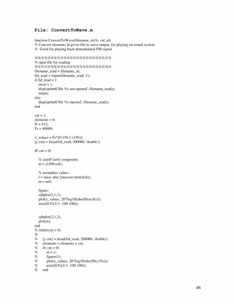
File: ConvertToWave.m function ConvertToWave(filename_in)%, val_id) % Convert elements in given file to wave output, for playing on sound system % Good for playing back demodulated FM signal %%%%%%%%%%%%%%%%%%%%%%%% % open file for reading %%%%%%%%%%%%%%%%%%%%%%%% filename_read = filename_in; fid_read = fopen(filename_read, 'r'); if fid_read < 1 error = 1; disp(sprintf('file %s not opened', filename_read)); return; else disp(sprintf('file %s opened', filename_read)); end cnt = 1; elements = 0; N = 512; Fs = 40000; x_values = Fs*[0:1/N:1-(1/N)]; [y cnt] = fread(fid_read, 200000, 'double'); if( cnt > 0) % cutoff early compoents m = y(500:cnt); % normalize values l = max( abs( [max(m) min(m)])); m = m/l; figure; subplot(2,1,1); plot(x_values, 20*log10(abs(fft(m,N)))); axis([0 Fs/2-1 -100 100]); subplot(2,1,2); plot(m); end % while(cnt > 0) % % [y cnt] = fread(fid_read, 200000, 'double'); % elements = elements + cnt; % if( cnt > 0) % m = y; % figure(1); % plot(x_values, 20*log10(abs(fft(y,N)))); % axis([0 Fs/2-1 -100 100]); % end

47

% % end disp(sprintf('read %d elements', elements)); fclose(fid_read); wavwrite(m,40000,sprintf('%s.wav',filename_read)); disp('finished reading elements'); File: process_file.m function [return_value] = process_file(filename_in, filename_out, frequency_center, Fs) % filename_in = 'fm95_5.dat'; % filename_out = 'as.dat'; % frequency_center = 7.15e6; % Fs = 20e6; %%%%%%%%%%%%%%%%%%%%%%%% % open file for reading %%%%%%%%%%%%%%%%%%%%%%%% filename_read = filename_in; fid_read = fopen(filename_read, 'r'); if fid_read < 1 error = 1; disp(sprintf('file %s not opened', filename_read)); return; else disp(sprintf('file %s opened', filename_read)); end %%%%%%%%%%%%%%%%%%%%%%%%% % open writing output to %%%%%%%%%%%%%%%%%%%%%%%%% filename_write = filename_out; fid_write = fopen(filename_write, 'w'); if fid_write < 1 error = 1; disp(sprintf('file %s not opened', filename_write)); return; else disp(sprintf('file %s opened', filename_write)); end %%%%%%%%%%%%%% % Parameters %%%%%%%%%%%%%% TRUE = 1; FALSE = 0; DFT_size = 1024*5; Sampling_Frequency = Fs; Samples_Per_Process = 40000; Do_DFT = TRUE;

48

return_value = -1; Fs = Sampling_Frequency; Samples = Samples_Per_Process; N = DFT_size; Center_Frequency = frequency_center; first_decimate = 125; second_decimate = 4; first_Fs = Fs/first_decimate; second_Fs = first_Fs/second_decimate; disp(sprintf('%s being processed', filename_in)); disp(sprintf('Fs = %d, Cf = %d', Sampling_Frequency, Center_Frequency)); disp(sprintf('CFIR = %d, quad_rate = %d', first_decimate, first_Fs)); disp(sprintf('RFIR = %d, audio_rate = %d', second_decimate, second_Fs)); last_read_size = 0; counter = 0; cnt = 1; c = 0; % [N_b,W_b] = buttord(0.16,0.22,0.5,40); % [B,A] = butter(N_b,W_b); [N_tv, W_tv] = buttord(0.03, 0.05, 0.01, 20); [B_tv, A_tv] = butter(N_tv,W_tv); % B_tv = fir1(N_tv, W_tv, 'low'); % A_tv = 1; % Quadrature Demodulation in one Line :-O z = exp([0:Samples-1]*2*pi*j*(Center_Frequency/Sampling_Frequency)); % z = real(z); dec_value = 1; normalized_once = FALSE; while( cnt>0) counter = counter + 1; [v cnt] = fread(fid_read, Samples, 'uint16'); last_read_size = last_read_size +cnt; if( normalized_once == FALSE ) normalized_once = TRUE; [y, slope, b]= normalize_data(v); else y = slope*v + b; end if( cnt > 0) %len = length(y); %v = [0:len-1]; % frequency shift q = z(1:length(y)).*y'; %r = abs(m);%decimate(m, 2);

49

r = filter(B_tv, A_tv, q); m = amplitude_demodulate(r); %m = decimate(m,dec_value); % m = decimate(q, first_decimate);%, 'FIR'); % %m = filter(B,A,m); % %phi = angle(x); % Get angle % %phi = angle(m); % % Do first difference using filtering [1 -1] % fm_vector = fm_demodulate(m); % % % %fm_vector = filter(B,A,fm_vector); % l = decimate(fm_vector, second_decimate);%, 'FIR'); c = fwrite(fid_write, m, 'double') + c; if( Do_DFT == TRUE ) figure(2); Fs = Sampling_Frequency; x_values = Fs*[0:1/N:1-(1/N)]; subplot(2,1,1), plot(x_values, 20*log10(abs(fft(y,N)))); %title(sprintf('%d/%d samples, step %d, Fs = %d', cnt, Samples, counter, Fs)); title('ntsc signal, 4Mhz IF carrier'); axis([0 Fs/2-1 0 100]); grid on; xlabel('Frequency (Hz)'); ylabel('Power(db)'); Fs = Sampling_Frequency; x_values = Fs*[0:1/N:1-(1/N)]; subplot(2,1,2), plot(x_values, 20*log10(abs(fft(m,N)))); axis([0 Fs/2-1 0 60]); grid on; xlabel('Frequency (Hz)'); ylabel('Power(db)'); figure(1); t = (1000/Fs)*[0:length(m) - 1]; plot(t, v); xlabel('ms'); axis([0 t(length(t)) 6.538e4 6.546e4]); title('time domain ntsc signal'); return end end end

50

disp(sprintf('counter = %d, %d element read', counter, last_read_size)); disp(sprintf('%d elements written to %s', c, filename_out)); % close file fclose(fid_read); fclose(fid_write); return_value = 1; return function [y, slope, b] = normalize_data(in) % map from max/min to -1 1 x1 = min(in); y1 = -1; x2 = max(in); y2 = 1; slope = (y1-y2)/(x1-x2); b = y1 - slope*x1; y = slope*in + b; return function [x] = amplitude_demodulate(y) x = abs(y); return % AKA Quadrature Detector function [x] = fm_demodulate(y) siz = length(y); lastVal = y(1); i = 0; while( siz > 0) i = i+1; siz = siz-1; val = y(i); product = val * conj(lastVal); lastVal = val; x(i) = angle(product); end return File: process_ntsc.m function process_ntsc(a) fid = fopen('ntsc_output.data', 'r'); if fid < 1 disp('couldnt open ntsc_output.data'); return; else disp('opened ntsc_output.data'); end

51

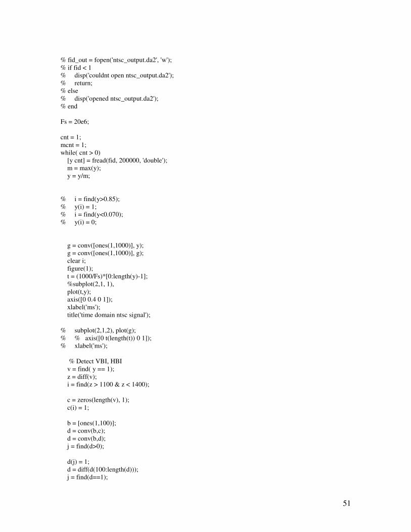
% fid_out = fopen('ntsc_output.da2', 'w'); % if fid < 1 % disp('couldnt open ntsc_output.da2'); % return; % else % disp('opened ntsc_output.da2'); % end Fs = 20e6; cnt = 1; mcnt = 1; while( cnt > 0) [y cnt] = fread(fid, 200000, 'double'); m = max(y); y = y/m; % i = find(y>0.85); % y(i) = 1; % i = find(y<0.070); % y(i) = 0; g = conv([ones(1,1000)], y); g = conv([ones(1,1000)], g); clear i; figure(1); t = (1000/Fs)*[0:length(y)-1]; %subplot(2,1, 1), plot(t,y); axis([0 0.4 0 1]); xlabel('ms'); title('time domain ntsc signal'); % subplot(2,1,2), plot(g); % % axis([0 t(length(t)) 0 1]); % xlabel('ms'); % Detect VBI, HBI v = find( y == 1); z = diff(v); i = find(z > 1100 & z < 1400); c = zeros(length(v), 1); c(i) = 1; b = [ones(1,100)]; d = conv(b,c); d = conv(b,d); j = find(d>0); d(j) = 1; d = diff(d(100:length(d))); j = find(d==1);

52

[mcnt] = get_syncs(y, v(i), v(j), mcnt); end fclose(fid); return; function [mcnt] = get_syncs(y, hsyncs_index, vsyncs_index, mcnt) for j = 1:length(vsyncs_index)-1, b = find( hsyncs_index > vsyncs_index(j)); b = min(b); cnt = 0; m = 0; r = cell(2,1); while( hsyncs_index(b) < vsyncs_index(j+1) ) aline = y( hsyncs_index(b):hsyncs_index(b+1)); if( length(aline) > m) m = length(aline); end b = b+1; cnt = cnt + 1; r{cnt} = aline; end save(sprintf('rframe%03d', mcnt), 'r'); disp(sprintf('wrote rframe%03d', mcnt)); mcnt = mcnt + 1; % g = get_picture(r); end return; function [g] = get_picture(r) % r = r(1:(length(r)-1)) % % % frame1 = cell(525,1); % % cnt = 0; % for i=1:length(r) % cnt = cnt + 1; % % if( length( r{cnt} ) < 1400) % frame1{cnt} = r{cnt}; % else % for j=0:ceil((length(r{cnt})/1250)-1)

53

% frame1{cnt} = r{j*1250+1:1250 + j*1250}; % % end % end % % end return File: process_ntsc_lines.m function [frame_out] = process_ntsc_lines (frame_in, std_size) % map from 1:1270 to 1:525 x1 = 1; x2 = 1270; y1 = 1; y2 = 525; m = (y1-y2)/(x1-x2); b = y1 - m*x1; for x=1:std_size; y = slope_intercept(m,b,x); frame_out(:,y) = frame_in(:,x); end return function [y] = slope_intercept(m,b,x) y = round(m*x + b); return File: process_frames.m function process_frames(a) clear all; close all; clc; Fs = 20e6; std_size = 63.5e-6*Fs; frame1 = []; last_frame = []; mov = avifile('my_rframes.avi'); mov.quality = 100; mov.fps = 10; mov.compression = 'Indeo5'; FALSE = 0;

54

TRUE = 1; first = TRUE; for frame_num = 1:103, load(sprintf('rframe%03d', frame_num)); disp(sprintf('reading rframe%03d', frame_num)); rf_len = length(r); frame1 = []; linecnt = 0; framecnt = 0; newline = 0; while linecnt < rf_len, linecnt = linecnt + 1; aline = r{linecnt}; len_aline = length(aline); for i=0:(round( length(aline)/std_size)-1), framecnt = framecnt + 1; frame1(framecnt, :) = ones(1,std_size); len_left = length( aline(i*std_size+1:len_aline)); if( len_left >= std_size) newline = aline(i*std_size+1:(i+1)*std_size); frame1(framecnt, :) = newline'; else newline = aline(i*std_size+1:len_aline); frame1(framecnt, 1:len_left) = newline'; end end end if( ~isempty(last_frame)) frame_out = merge_frames(last_frame, frame1, std_size); frame_out = process_ntsc_lines(frame_out, std_size); if( first == TRUE ) [row,col] = size(frame_out); row = row - 20; col = col - 20; first = FALSE; end h = figure(1);imshow(frame_out(1:row,1:col)); title(sprintf('frame %03d', frame_num));

55

F = getframe(gca); mov = addframe(mov,F); end last_frame = frame1; end mov = close(mov); File: merge_frames.m function [frame_out] = merge_frames(frame1, frame2, std_size) [len1,c] = size(frame1); [len2,c] = size(frame2); lmax = max([len1 len2]); frame_out = ones(lmax*2, std_size); jcnt = 0; for i=1:lmax, if( i <= len1 ) frame_out(i*2-1,:) = frame1(i,:); end if( i <= len2 ) frame_out(i*2 ,:) = frame2(i,:); end end return File: ReadFM95_5.m function ReadFM95() clear all; close all; clc; % % disp('before file naming'); % pause; %%%%%%%%%%%%%%%%%%%%%%%% % open file for reading %%%%%%%%%%%%%%%%%%%%%%%% filename_read = 'fm95_5.dat'; filename_write1 = '7_15.dat'; freq1 = 7.15e6; filename_write2 = '5_75.dat'; freq2 = 5.75e6; filename_write3 = '2_95.dat'; freq3 = 2.95e6; % disp('before file processing'); % pause;

56

sampling_frequency = 20e6; filename_out = filename_write1; freq = freq1; val = 1; r = process_file(filename_read, filename_out, freq, sampling_frequency); disp(sprintf('%s = %d', filename_out, r)); % ConvertToWave(filename_out, val); % % filename_out = filename_write2; % freq = freq2; % val = 2; % r = process_file(filename_read, filename_out, freq, sampling_frequency); % disp(sprintf('%s = %d', filename_out, r)); % ConvertToWave(filename_out, val); % % filename_out = filename_write3; % freq = freq3; % val = 3 % r = process_file(filename_read, filename_out, freq, sampling_frequency); % disp(sprintf('%s = %d', filename_out, r)); % ConvertToWave(filename_out, val); File: Readntsc.m function DoNTSC(y) filename_read = 'ntsc.dat'; filename_write1 = 'ntsc_output.data'; freq1 = 4e6; filename_write2 = 'b.dat'; freq2 = 8.57e6; filename_write3 = 'd.dat'; freq3 = 4.75e6; global van; van = 1; sampling_frequency = 20e6; r = process_file(filename_read, filename_write1, freq1, sampling_frequency); disp(sprintf('%s = %d', filename_write1, r)); % r = process_file(filename_read, filename_write2, freq2, sampling_frequency);; % disp(sprintf('%s = %d', filename_write2, r)); % % % r = process_file(filename_read, filename_write3, freq3, sampling_frequency); % disp(sprintf('%s = %d', filename_write3, r)); File: sine_wave_test.m close all; clear all; clc; fs = 44.1e3; % fs = 44.1Khz

57

t_total = 2; % number of seconds of data n_samples = fs*t_total; % number of samples % Generated frequencies f1 = 5000; % Frequency generated f2 = 0; step_size = 1/fs; t = 0:step_size:t_total-step_size; % time of the samples y1 = sin(2*pi*f1*t); % generate wave y2 = sin(2*pi*f2*t); y = y1 + y2; s = 1024; m = s/2; c = (1/s)*[0:s-1]*(fs/1000); Y = ( abs( fft(y,s) )); plot(c(1:m),Y(1:m)); ylabel('Magnitude'); xlabel('Frequency (kHz)'); wavplay(y,fs);

58

59

Appendix D: Special Resources http://www.gnu.org/software/gnuradio/gnuradio.html www.ti.com www.rfmicro.com

60

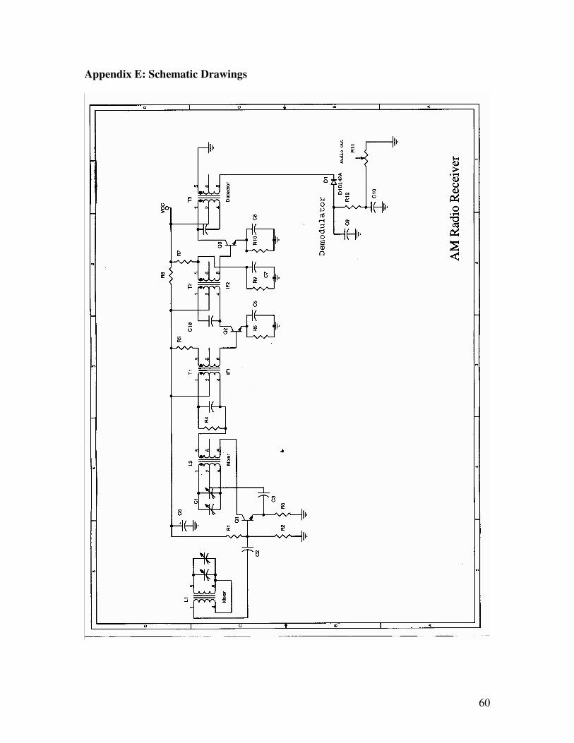
Appendix E: Schematic Drawings

61

62

63

64

Appendix F: Pictures of Receiver and Quadrature Demodulator

Audio Amplfier

Quadrature Demodulator

65

FM Front End: