Embed Size (px)
Citation preview
Scilab Codes forDigital Signal Processingby Proakis and Manolakis1
Created byHasan Ali Stationwala
B.Tech., 2nd Year StudentElectronics and Communication Engineering,
National Institute Of Technology,Tiruchirappalli
College teacherMadhu N. Belur, IIT Bombay
ReviewerPrashant Dave, IIT Bombay
15 July, 2010
1Funded by a grant from the National Mission on Education through ICT,http://spoken-tutorial.org/NMEICT-Intro
Book Details
Authors: Proakis and Manolakis
Title: Digital Signal Processing: Principle, algorithms and applications
Publisher: Dorling Kindersley India Pvt. Ltd.(licensees of Prentice Education in South Asia)
Edition: 4th
Year: 2007
Place: New Delhi
Scilab numbering policy used in this document and the relation to the abovebook is as follows.
Prb Problem (Unsolved problem) These are at the end of each chapter.
Exa Example (Solved example)
Sec Section (Particular section of the above book)
For example, Prb 2.67 means Problem 2.67 of the above book. Scilab codehaving number Sec 2.6 means a scilab code whose theory is explained inSection 2.6 of the book.
1
Contents
List of Scilab Codes 4
2 Impulse Response and Correlation 22.4 Impulse response . . . . . . . . . . . . . . . . . . . . . . . . 22.66 Problem . . . . . . . . . . . . . . . . . . . . . . . . . . . . . 32.67 Problem . . . . . . . . . . . . . . . . . . . . . . . . . . . . . 52.6 Correlation . . . . . . . . . . . . . . . . . . . . . . . . . . . 62.65 Problem . . . . . . . . . . . . . . . . . . . . . . . . . . . . . 8
5 Quantization and Filter Design by placing poles and zeros 155.1 Function “quantize()” . . . . . . . . . . . . . . . . . . . . . 155.14 Problem . . . . . . . . . . . . . . . . . . . . . . . . . . . . . 175.4 Filter Design by placing poles and zeros . . . . . . . . . . . 185.43 Problem . . . . . . . . . . . . . . . . . . . . . . . . . . . . . 18
8 The discrete fourier transform (DFT) and the fast fouriertransform (FFT) 208.1 Function “mydft()” . . . . . . . . . . . . . . . . . . . . . . . 208.2 Function “divdft()” . . . . . . . . . . . . . . . . . . . . . . . 218.3 Function “r2fft()” . . . . . . . . . . . . . . . . . . . . . . . . 238.36 Problem . . . . . . . . . . . . . . . . . . . . . . . . . . . . . 24
9 Implementation of FIR and IIR filters 279.2 Function “direct1()”, ”lattfir()” and ”lattimpulse()” . . . . . 27
9.2.1 Function ”direct()” . . . . . . . . . . . . . . . . . . . 279.2.4 Function “lattfir()” . . . . . . . . . . . . . . . . . . . 29
9.3 Function ”lattimpulse()” . . . . . . . . . . . . . . . . . . . . 309.4 Function “lattladd()” and ”llimpulse()” . . . . . . . . . . . . 31
2
9.40 Problem . . . . . . . . . . . . . . . . . . . . . . . . . . . . . 34
10 FIR and IIR Filter Design 3610.2 FIR filter design by window method . . . . . . . . . . . . . . 3610.3 IIR fiter design by Butterworth filter design and Bi-linear
Transformation . . . . . . . . . . . . . . . . . . . . . . . . . 40
Solved examples from book’s appendix 45
3
List of Scilab Codes
Sec 2.4 Impulse.sce . . . . . . . . . . . . . . . . . . . . . . . . 2Prb 2.66 Impulse.sce . . . . . . . . . . . . . . . . . . . . . . . . 3Prb 2.67 Problem 2.67 . . . . . . . . . . . . . . . . . . . . . . . 5Sec 2.6 Correlation . . . . . . . . . . . . . . . . . . . . . . . . 7Prb 2.65 Problem 2.65 . . . . . . . . . . . . . . . . . . . . . . . 8Sec 5.14 quantize.sce . . . . . . . . . . . . . . . . . . . . . . . . 15Prb 5.14 Problem 5.14 . . . . . . . . . . . . . . . . . . . . . . . 17Prb 5.43 5.43.sce . . . . . . . . . . . . . . . . . . . . . . . . . . 18Sec 8.1 mydft.sce . . . . . . . . . . . . . . . . . . . . . . . . . 20Sec 8.2 divdft.sce . . . . . . . . . . . . . . . . . . . . . . . . . 22Sec 8.3 r2fft.sce . . . . . . . . . . . . . . . . . . . . . . . . . . 24Prb 8.36 Problem 8.36 . . . . . . . . . . . . . . . . . . . . . . . 24Prb 8.36 Problem 8.36 . . . . . . . . . . . . . . . . . . . . . . . 25Sec 9.2 direct1.sce . . . . . . . . . . . . . . . . . . . . . . . . 28Sec 9.2 lattfir.sce . . . . . . . . . . . . . . . . . . . . . . . . . 29Sec 9.2 lattimpulse.sce . . . . . . . . . . . . . . . . . . . . . . 30Sec 9.3 lattladd.sce . . . . . . . . . . . . . . . . . . . . . . . . 32Sec 9.3 llimpulse.sce . . . . . . . . . . . . . . . . . . . . . . . 33Prb 9.40 Problem . . . . . . . . . . . . . . . . . . . . . . . . . . 34Sec 10.2 Low pass FIR filter . . . . . . . . . . . . . . . . . . . . 37Sec 10.2 High pass FIR filter . . . . . . . . . . . . . . . . . . . 38Sec 10.2 Bandpass FIR filter . . . . . . . . . . . . . . . . . . . 38Sec 10.2 Bandstop FIR filter . . . . . . . . . . . . . . . . . . . 39Sec 10.3 buttordc.sce . . . . . . . . . . . . . . . . . . . . . . . 41Sec 10.3 buttord.sce . . . . . . . . . . . . . . . . . . . . . . . . 42Sec 10.3 butterc.sce . . . . . . . . . . . . . . . . . . . . . . . . 42Sec 10.3 butterd.sce . . . . . . . . . . . . . . . . . . . . . . . . 43Exa 16 Example 16, page 1098 . . . . . . . . . . . . . . . . . 45
4

Exa 17 Example 17, page no. 1103 . . . . . . . . . . . . . . . 45Exa 18 Example 18, page no. 1104 . . . . . . . . . . . . . . . 45Exa 25 Example 25, page no. 1114 . . . . . . . . . . . . . . . 46Exa 25 Example 29, page no. 1120 . . . . . . . . . . . . . . . 46
5
List of Figures
2.1 Problem 2.66 . . . . . . . . . . . . . . . . . . . . . . . . . . 112.2 Problem 2.66 . . . . . . . . . . . . . . . . . . . . . . . . . . 122.3 Problem 2.66 . . . . . . . . . . . . . . . . . . . . . . . . . . 132.4 Problem 2.65 . . . . . . . . . . . . . . . . . . . . . . . . . . 14
1
Chapter 2
Impulse Response andCorrelation
2.4 Impulse response
When unit impulse is fed as input, the output of the system is called as theimpulse response of the system. It is usually denoted by h(n). This functioncalculates the impulse response of system described by following differenceequation:
y(n) = a1y(n−1)+a2y(n−2)+a3y(n−3)...+b0x(n)+b1x(n−1)+b2x(n−2)...(2.1)
This function takes following parameters as arguments:
• a-array of a1, a2... (a row vector)
• b-array of b0, b1, b2... (a row vector)
• n-size of impulse response (a scalar)
it is assumed that size of a is greater than size of b
Scilab code Sec 2.41 / / f u n c t i o n t o c a l a i m p u l s e r e s p o n s e o f
g i v e n d i f f e q .
2 / / i n p u t s a , b ( r o w v e c t o r s ) a n d %n ( s c a l a r )
3
2
4 function h=impulse ( a , b ,%n)5
6 %a=length ( a ) ;7
8 / / z e r o − p a d d i n g i n o r d e r t o m a k e e l e m e n t w i s e s u m m a t i o n
c o m p a t i b l e
9 [ b ]=[b , zeros (1 ,%n−length (b) ) ] ;10 h=[zeros ( 1 , 1 ) ] ;11 h (1 , 1 )=b (1 , 1 ) ;12 %index=2;13
14 / / c o m p u t i n g f i r s t %a t e r m s
15 while %index <= %a,16 h (1 , %index )=−a ( 1 , 1 : %index−1)∗(h (1 , %index−1:−1:1) . ’ )+b
(1 , %index ) ;17 %index=%index+1;18 end19
20 / / c o m p u t a t i o n o f t e r m s a f t e r f i r s t %a t e r m s
21 while %index <= %n,22 h (1 , %index )=−a ( 1 , 1 : $ )∗h (1 , $ :−1:$−%a+1) . ’+b (1 , %index ) ;23 %index=%index+1;24 end25
26 endfunction
2.66 Problem
Scilab code Prb 2.661 / / P r o b l e m 2 . 6 6 D i g i t a l S i g n a l
P r o c e s s i n g b y P r o a k i s M a n o l a k i s F o u r t h E d i t i o n
2 a=[−0.8 , 0 . 6 4 ] ;3 b = [ 0 . 8 6 6 ] ;4
5 / / l e n g t h o f r e s p o n s e
6 %n=50;7
3
8 %a=length ( a ) ;9 / / z e r o − p a d d i n g i n o r d e r t o m a k e e l e m e n t w i s e s u m m a t i o n
c o m p a t i b l e
10 b=[b , zeros (1 ,%n−length (b) ) ] ;11 h=[zeros ( 1 , 1 ) ] ;12 h (1 , 1 )=b (1 , 1 ) ;13 %index=2;14
15 / / c o m p u t i n g f i r s t %a t e r m s
16 while %index <= %a,17 h (1 , %index )=−a ( 1 , 1 : %index−1)∗h (1 , %index−1:−1:1) . ’+b
(1 , %index ) ;18 %index=%index+1;19 end20
21 / / c o m p u t a t i o n o f t e r m s a f t e r f i r s t %a t e r m s
22 while %index <= %n,23 h (1 , %index )=−a ( 1 , 1 : $ )∗h (1 , $ :−1:$−%a+1) . ’+b (1 , %index
) ;24 %index=%index+1;25 end26
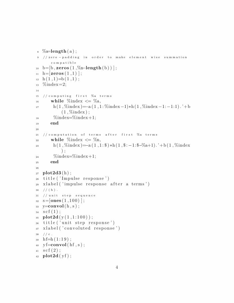
27 plot2d3 (h) ;28 t i t l e ( ’ Impulse re sponse ’ )29 x l a b e l ( ’ impulse re sponse a f t e r a terms ’ )30 / / ( b ) .
31 / / u n i t s t e p s e q u e n c e
32 s =[ones (1 ,100) ] ;33 y=convol (h , s ) ;34 s c f (1 ) ;35 plot2d ( y ( 1 , 1 : 1 0 0 ) ) ;36 t i t l e ( ’ un i t s tep response ’ )37 x l a b e l ( ’ convoluted response ’ )38 / / c .
39 hf=h ( 1 : 1 9 ) ;40 yf=convol ( hf , s ) ;41 s c f (2 ) ;42 plot2d ( y f ) ;
4
43 t i t l e ( ’ un i t s tep response ’ )44 x l a b e l ( ’ convoluted response ’ )45 / / p l o t w i t h t h e p i l l a r s i s i m p u l s e r e s p o n s e a n d t h a t
w i t h s m o o t h c u r v e i s u n i t s t e p r e s p o n s e
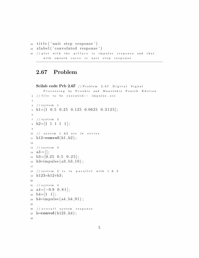
2.67 Problem
Scilab code Prb 2.671 / / P r o b l e m 2 . 6 7 D i g i t a l S i g n a l
P r o c e s s i n g b y P r o a k i s a n d M a n o l a k i s F o u r t h E d i t i o n
2 / / f i l e t o b e e x e c u t e d : − i m p u l s e . s c e
3
4 / / s y s t e m 1
5 h1=[1 0 .5 0 .25 0 .125 0 .0625 0 . 3 1 2 5 ] ;6
7 / / s y s t e m 2
8 h2=[1 1 1 1 1 ] ;9
10 / / s y s t e m 1 &2 a r e i n s e r i e s
11 h12=convol ( h1 , h2 ) ;12
13 / / s y s t e m 3
14 a3 = [ ] ;15 b3 =[0.25 0 .5 0 . 2 5 ] ;16 h3=impulse ( a3 , b3 , 1 0 ) ;17
18 / / s y s t e m 3 i s i n p a r a l l e l w i t h 1 & 2
19 h123=h12+h3 ;20
21 / / s y s t e m 4
22 a4=[−0.9 0 . 8 1 ] ;23 b4=[1 1 ] ;24 h4=impulse ( a4 , b4 , 9 1 ) ;25
26 / / o v e r a l l s y s t e m r e s p o n s e
27 h=convol ( h123 , h4 ) ;28
5
29 plot2d3 (h) ;
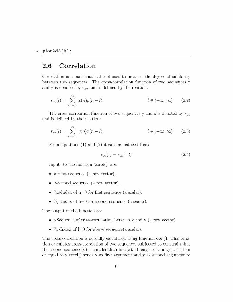
2.6 Correlation
Correlation is a mathematical tool used to measure the degree of similaritybetween two sequences. The cross-correlation function of two sequences xand y is denoted by rxy and is defined by the relation:
rxy(l) =∞∑
n=−∞x(n)y(n− l), l ∈ (−∞,∞) (2.2)
The cross-correlation function of two sequences y and x is denoted by ryxand is defined by the relation:
ryx(l) =∞∑
n=−∞y(n)x(n− l), l ∈ (−∞,∞) (2.3)
From equations (1) and (2) it can be deduced that:
rxy(l) = ryx(−l) (2.4)
Inputs to the function ’corel()’ are:
• x-First sequence (a row vector).
• y-Second sequence (a row vector).
• %x-Index of n=0 for first sequence (a scalar).
• %y-Index of n=0 for second sequence (a scalar).
The output of the function are:
• r-Sequence of cross-correlation between x and y (a row vector).
• %r-Index of l=0 for above sequence(a scalar).
The cross-correlation is actually calculated using function cor(). This func-tion calculates cross-correlation of two sequences subjected to constrain thatthe second sequence(y) is smaller than first(x). If length of x is greater thanor equal to y corel() sends x as first argument and y as second argument to
6
cor(). But if length of x is smaller than y, it sends y as first argument andx as second argument to cor(), i.e. cor() actually calculates ryx and thencorel() calculates rxy from ryx using relation above.
The function ’cor()’ calculates cross-correlation between two sequences,with constraint that the second sequence should be smaller than the firstsequence. Inputs to the function are:
• x-First sequence (a row vector)
• y-Second sequence (a row vector)
The output of the function is:
• r-The cross-correlation sequence (a row vector)
The lth term of cross-correlation of two sequences is calculated first byshifting second sequence by l units.
Scilab code Sec 2.61 / / f u n c t i o n t o c a l c u l a t e c o r r e l a t i o n b e t w e e n s i g n a l s
2 / / i n p u t s : − x , y t w o r o w v e c t o r s , %x , %y t w o s c a l a r s
3 / / o u t p u t s : −R r o w v e c t o r , %R s c a l a r
4
5 function [R,%R]= c o r e l (x , y ,%x,%y)6
7 %R=length ( y )−%y+%x; / / c a l c u l a t i n g i n d e x o f l =0 i n R
8 i f ( length ( x )>=length ( y ) )9 R=cor (x , y ) ; / / c a l c u l a t i n g o f R x y
10 else11 R=cor (y , x ) ; / / c a l c u l a t i n g R y x
12 R=R(1 , $ :−1:1) ; / / r e v e r s i n g t h e s e q u e n c e f o r R x y
13 end14
15 endfunction16
17
18 / / f u n c t i o n t o f i n d c o r e l a t i o n
19
20 function R= cor (a , b)
7
21
22 R=[zeros (1 , length ( a )+length (b)−1) ] ;23 %r=length (b)−1;24
25 %index=0;26 while %index<=(length (b)−1) ; / / c a l c u l a t i n g f i r s t
l e n g t h ( b ) t e r m s
27 r=a ( 1 , 1 : ( %index+1) ) .∗b (1 , $−%index : $ ) ; / / s h i f t i n g
a n d m u l t i p l i c a t i o n
28 R(1 , %index+1)=sum( r , 2 ) ; / / a d d i t i o n
29 %index=%index+1;30 end31
32 %index=1;33 while %index<=(length ( a )−length (b) ) ; / / c a l c u l a t i n g
n e x t l e n g t h ( a ) t e r m s
34 r=b ( 1 , 1 : $ ) .∗ a (1 , %index+1: length (b)+%index ) ;35 R(1 , %index+length (b) )=sum( r , 2 ) ;36 %index=%index+1;37 end38
39 %index=1; / / c a l c u l a t i n g r e m a i n i n g t e r m s
40 while %index<=(length (b)−1) ,41 r=b ( 1 , 1 : $−%index ) .∗ a (1 , $−length (b)+%index+1:$ ) ;42 R(1 , %index+length ( a ) )=sum( r , 2 ) ;43 %index=%index+1;44 end45
46 endfunction
2.65 Problem
Scilab code Prb 2.651 / / P r o b l e m 2 . 6 5 d i g i t a l s i g n a l
p r o c e s s i n g b y P r o a k i s a n d M a n o l a k i s F o u r t h e d i t i o n
2 / / f i l e t o b e e x e c u t e d : − c o r e l . s c e
3 / / t h e d e l a y ’ d ’ c a n b e e s t i m a t e d b y c a l c u l a t i n g
8
4 / / c r o s s c o r r e l a t i o n b e t w e e n r e c e i v e d s i g n a l &
t r a n s m i t t e d s i g n a l .
5 / / A u t o c o r r e l a t i o n o f t r a n s m i t t e d s i g n a l
6 / / d i s t a n c e b e t w e e n t h e p e e k s o f t w o p l o t s g i v e s t h e
d e l a y
7
8
9 / / ( b )
10
11 / / t r a n s m i t t e d s e q u e n c e
12 x=[1 1 1 1 1 −1 −1 1 1 −1 1 −1 1 ] ;13
14 / / n o i s e s e q u e n c e
15 v=grand (1 ,200 , ”nor” , 0 , 0 . 0 1 ) ;16
17 / / r e c e i v e d s e q u e n c e
18 y =0.9∗ [ zeros (1 , 20 ) x zeros (1 , length ( v )−20−length ( x ) ) ]+v;
19
20 / / c a l c u l a t i n g r y x
21 [ r , %r]= c o r e l (y , x , 0 , 0 ) ;22
23 / / s e l e c t i n g f i r s t 5 9 t e r m s
24 r =[ r (1 ,%r : %r+59) ] ;25
26 / / p l o t t i n g
27 plot2d3 ( r )28 t i t l e ( ’ c r o s s c o r r e l a t i o n between r e c e i v e d s i g n a l and
transmit ted s i g n a l ’ )29 x l a b e l ( ’ r−c r o s s c o r r e l a t i o n sequence ’ )30
31
32 / / P e a k o f t h i s f u n c t i o n i s a t n = 2 0 w h i c h i s e x p e c t e d
33 / / w h e n v a l u e o f v a r i a n c e i s i n c r e a s e d i n l i n e n o 1 3 (
f o u r t h a r g u m e n t o f f u n c t i o n g r a n d ( ) ) t h e p e a k
b e c o m e s l e s s d o m i n a n t
34 / / h e n c e t h e v a l u e o f d e l a y c a n b e e s t i m a t e d p r o p e r l y
o n l y i f v a r i a n c e o f n o i c e i s k e p t l o w .
9

10
Figure 2.1: Problem 2.66
11
Figure 2.2: Problem 2.66
12
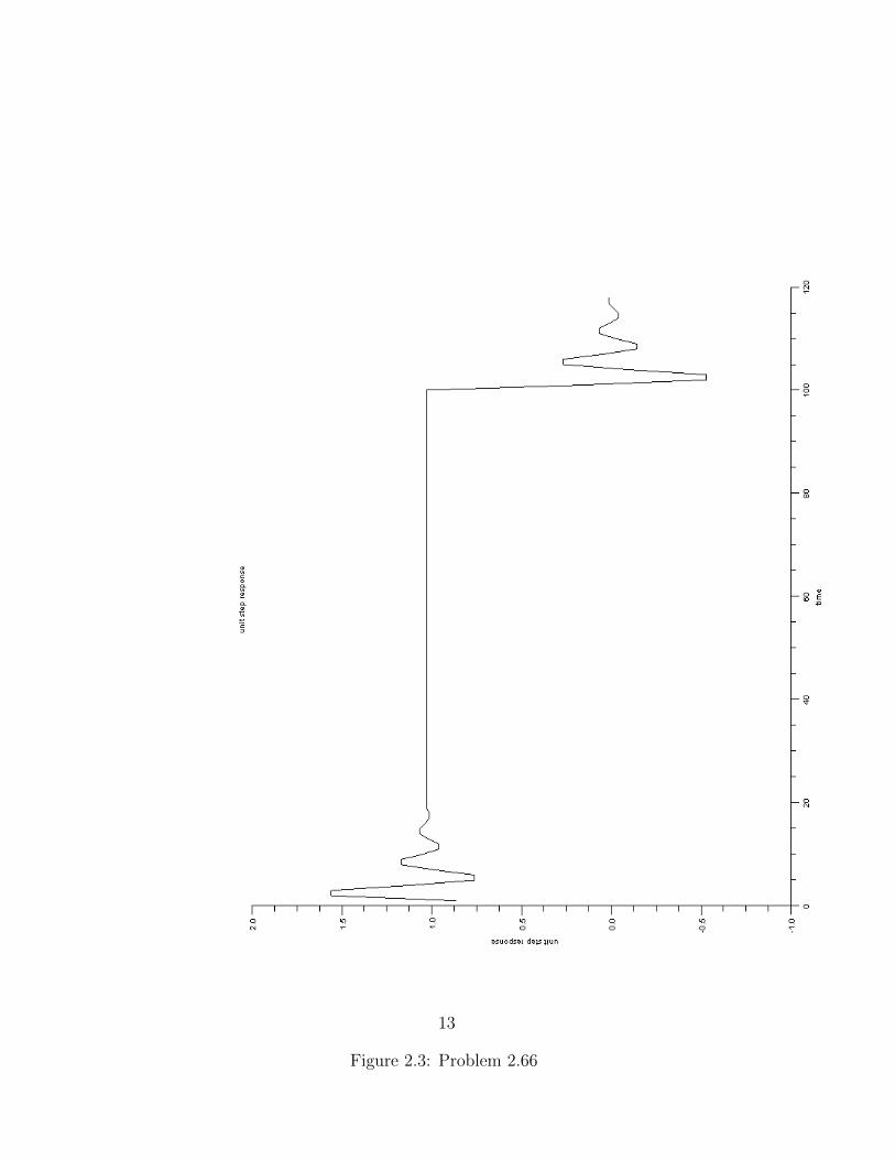
Figure 2.3: Problem 2.66
13
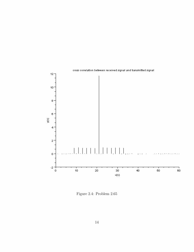
Figure 2.4: Problem 2.65
14
Chapter 5
Quantization and Filter Designby placing poles and zeros
5.1 Function “quantize()”
In the code presented here, the given sequence is quantized to desired numberof bits. Inputs to the function ’quantize()’ are:
• x-the sequence to be quantized (a row vector)
• b-no. of bits (a scalar)
• max-maximum value in given sequence (a scalar)
• min- minimum value in given sequence (a scalar)
Output is:
• xq-the quantized sequence (a row vector).
The function first finds two consecutive quantization levels within which aparticular element falls, then it checks if that element falls above or belovecorresponding decision level.
Scilab code Sec 5.141 / / f u n c t i o n t o q u a n t i z e g i v e n s e q u e n c e
2 / / i n p u t s : x , ( a r o w v e c t o r ) ; b , mx , mn ( a l l s c a l a r s )
3 / / o u t p u t : x q , ( a r o w v e c t o r )
15
4
5 function xq=quant ize (x , b ,mx,mn)6
7 / / l e v e l s
8 l =2ˆb ;9
10 / / s t e p s i z e
11 s=(mx−mn) / l ;12
13 / / q u a n t i z a t i o n l e v e l s
14 q l =[mn: s :mx ] ;15
16 / / d i c e s i o n l e v e l s
17 dl =[mn+(s /2) : s :mx ] ;18 index =1;19 xq = [ ] ;20
21 while index<=length ( x )22 count =2;23 while count<=length ( q l )24 i f x ( index )>q l ( count )25 count=count +1;26 cont inue27 else28 i f x ( index )<=dl ( count−1)29 xq (1 , index )=q l ( count−1) ;30 else31 xq (1 , index )=q l ( count ) ;32 end33 end34 break ;35 end36 index=index +1;37 end38
39 endfunction
16
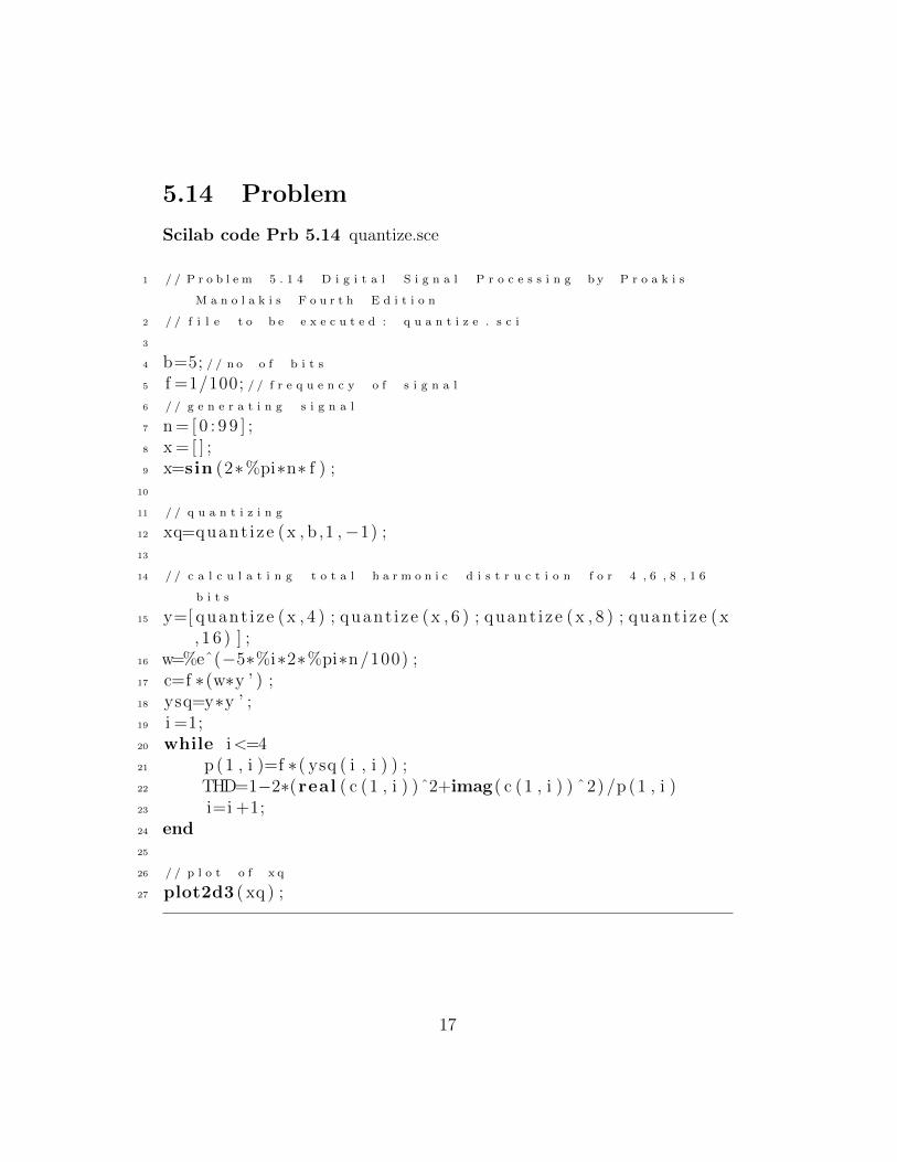
5.14 Problem
Scilab code Prb 5.14 quantize.sce
1 / / P r o b l e m 5 . 1 4 D i g i t a l S i g n a l P r o c e s s i n g b y P r o a k i s
M a n o l a k i s F o u r t h E d i t i o n
2 / / f i l e t o b e e x e c u t e d : q u a n t i z e . s c i
3
4 b=5; / / n o o f b i t s
5 f =1/100; / / f r e q u e n c y o f s i g n a l
6 / / g e n e r a t i n g s i g n a l
7 n = [ 0 : 9 9 ] ;8 x = [ ] ;9 x=sin (2∗%pi∗n∗ f ) ;
10
11 / / q u a n t i z i n g
12 xq=quant ize (x , b ,1 ,−1) ;13
14 / / c a l c u l a t i n g t o t a l h a r m o n i c d i s t r u c t i o n f o r 4 , 6 , 8 , 1 6
b i t s
15 y=[ quant i ze (x , 4 ) ; quant i ze (x , 6 ) ; quant i ze (x , 8 ) ; quant i ze (x, 1 6 ) ] ;
16 w=%eˆ(−5∗%i∗2∗%pi∗n/100) ;17 c=f ∗(w∗y ’ ) ;18 ysq=y∗y ’ ;19 i =1;20 while i<=421 p (1 , i )=f ∗( ysq ( i , i ) ) ;22 THD=1−2∗(real ( c (1 , i ) )ˆ2+imag( c (1 , i ) ) ˆ2) /p (1 , i )23 i=i +1;24 end25
26 / / p l o t o f x q
27 plot2d3 ( xq ) ;
17
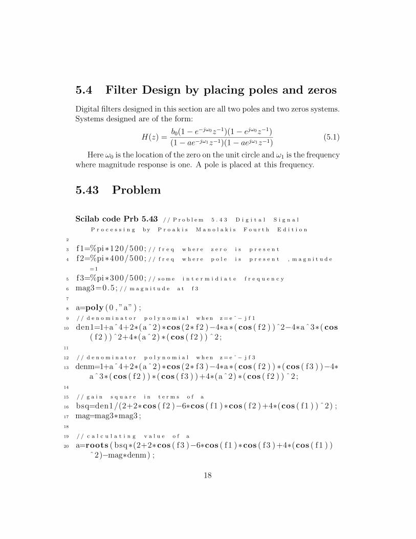
5.4 Filter Design by placing poles and zeros
Digital filters designed in this section are all two poles and two zeros systems.Systems designed are of the form:
H(z) =b0(1− e−jω0z−1)(1− ejω0z−1)
(1− ae−jω1z−1)(1− aejω1z−1)(5.1)
Here ω0 is the location of the zero on the unit circle and ω1 is the frequencywhere magnitude response is one. A pole is placed at this frequency.
5.43 Problem
Scilab code Prb 5.431 / / P r o b l e m 5 . 4 3 D i g i t a l S i g n a l
P r o c e s s i n g b y P r o a k i s M a n o l a k i s F o u r t h E d i t i o n
2
3 f 1=%pi∗120/500; / / f r e q w h e r e z e r o i s p r e s e n t
4 f 2=%pi∗400/500; / / f r e q w h e r e p o l e i s p r e s e n t , m a g n i t u d e
=1
5 f 3=%pi∗300/500; / / s o m e i n t e r m i d i a t e f r e q u e n c y
6 mag3=0.5; / / m a g n i t u d e a t f 3
7
8 a=poly (0 , ”a” ) ;9 / / d e n o m i n a t o r p o l y n o m i a l w h e n z = e ˆ− j f 1
10 den1=1+aˆ4+2∗(a ˆ2)∗cos (2∗ f 2 )−4∗a∗( cos ( f 2 ) )ˆ2−4∗a ˆ3∗( cos( f 2 ) ) ˆ2+4∗(a ˆ2) ∗( cos ( f 2 ) ) ˆ2 ;
11
12 / / d e n o m i n a t o r p o l y n o m i a l w h e n z = e ˆ− j f 3
13 denm=1+aˆ4+2∗(a ˆ2)∗cos (2∗ f 3 )−4∗a∗( cos ( f 2 ) ) ∗( cos ( f 3 ) )−4∗a ˆ3∗( cos ( f 2 ) ) ∗( cos ( f 3 ) ) +4∗(a ˆ2) ∗( cos ( f 2 ) ) ˆ2 ;
14
15 / / g a i n s q u a r e i n t e r m s o f a
16 bsq=den1/(2+2∗cos ( f 2 )−6∗cos ( f 1 )∗cos ( f 2 ) +4∗(cos ( f 1 ) ) ˆ2) ;17 mag=mag3∗mag3 ;18
19 / / c a l c u l a t i n g v a l u e o f a
20 a=roots ( bsq∗(2+2∗cos ( f 3 )−6∗cos ( f 1 )∗cos ( f 3 ) +4∗(cos ( f 1 ) )ˆ2)−mag∗denm) ;
18
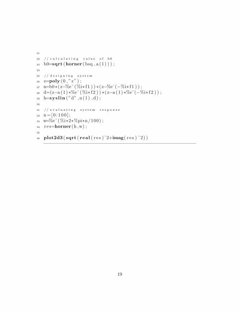
21
22 / / c a l c u l a t i n g v a l u e o f b 0
23 b0=sqrt (horner ( bsq , a (1 ) ) ) ;24
25 / / d e s i g n i n g s y s t e m
26 z=poly (0 , ”z” ) ;27 n=b0∗( z−%eˆ(%i∗ f 1 ) ) ∗( z−%eˆ(−%i∗ f 1 ) ) ;28 d=(z−a (1 ) ∗%eˆ(%i∗ f 2 ) ) ∗( z−a (1 ) ∗%eˆ(−%i∗ f 2 ) ) ;29 h=sysl in ( ”d” ,n (1 ) ,d ) ;30
31 / / e v a l u a t i n g s y s t e m r e s p o n s e
32 n = [ 0 : 1 0 0 ] ;33 w=%eˆ(%i∗2∗%pi∗n/100) ;34 r e s=horner (h ,w) ;35
36 plot2d3 ( sqrt ( real ( r e s )ˆ2+imag( r e s ) ˆ2) )
19
Chapter 8
The discrete fourier transform(DFT) and the fast fouriertransform (FFT)
In this section functions are defined to calculate discrete fourier transform ofgiven sequence.These functions are:-
• mydft()-This function calculates the dft by its definition.
• divdft()-Calculation of dft by divide and conquer approach.
• r2fft()-Calculation of dft by radix 2 method.
8.1 Function “mydft()”
This function calculates the dft of a sequence by its definition and thereforenot the efficient manner to calculate the dft.The input to the function is:
• x:-The sequence of which the dft is to be calculated (a row vector)
The output of the function is:
• X:-The dft of the sequence (a row vector)
20
Scilab code Sec 8.11 / / f u n c t i o n t o c o m p u t e d f t o f a s e q u e n c e
2 / / i n p u t : x ( a r o w v e c t o r )
3 / / o u t p u t : X ( a r o w v e c t o r )
4
5 function X=mydft ( x )6
7 %n=length ( x ) ;8 w=%eˆ(−%i∗2∗%pi/%n) ;9 k=0;
10
11 / / f o r m a t i o n o f t h e W m a t r i x
12 while k<%n13 n=0;14 while n<%n15 W(n+1,k+1)=wˆ( k∗n) ;16 n=n+1;17 end18 k=k+1;19 end20
21 X=x∗W;22
23 endfunction
8.2 Function “divdft()”
This function calculates the dft by divide and conquer approach.The lengthof the sequence should be compulsorily m times l. The actual sequence isfirst arranged column-wise in ’l’ rows and ’m’ columns to form a matrix, thenthe ’m’ point dft of each row is calculated. Each element of this calculateddft is multiplied by an appropriate phase factor and again ’l’ point dft ofeach column of resultant matrix is calculated using function mydft(). Thematrix obtained when read row-wise gives the dft.This concept is explained in detail in Digital Signal Processing by Proakisand Manolakis Fourth Edition.The inputs to the function are:
21

• x-the sequnce (a row vector)
• l-no of columns (a scalar)
• m-no of rows (a scalar)
The output of the function is:
• X-DFT of given sequence (row vector)
Scilab code Sec 8.21 / / f u n c t i o n t o c a l c u l a t e f f t b y d i v i d e
a n d c o n q u e r a p p r o a c h
2 / / i n p u t s : x ( a r o w v e c t o r ) a n d m , l ( s c a l a r s )
3 / / o u t p u t : X ( a r o w v e c t o r )
4
5 function X=d i v d f t (x , l ,m)6
7 w=%eˆ(−%i∗2∗%pi/( l ∗m) ) ;8 %m=0;9
10 / / f o r m a t i o n o f l c r o s s m m a t r i x
11 while %m<m12 %l=0;13 while %l<l14 XX(%l+1,%m+1)=x (%l+1+%m∗ l ) ;15 %l=%l+1;16 end17 %m=%m+1;18 end19 %l=0;20
21 / / d f t ’ s o f r o w v e c t o r s a n d m u l t i p l y i n g w i t h p h a s e
f a c t o r
22 while %l<l23 %m= [ ] ;24 %m=[0:m−1] ;25 XX(%l +1 , : )=mydft (XX(%l +1 , : ) ) ;26 XX(%l +1 , : )=XX(%l +1 , : ) .∗wˆ(%l∗%m) ;
22
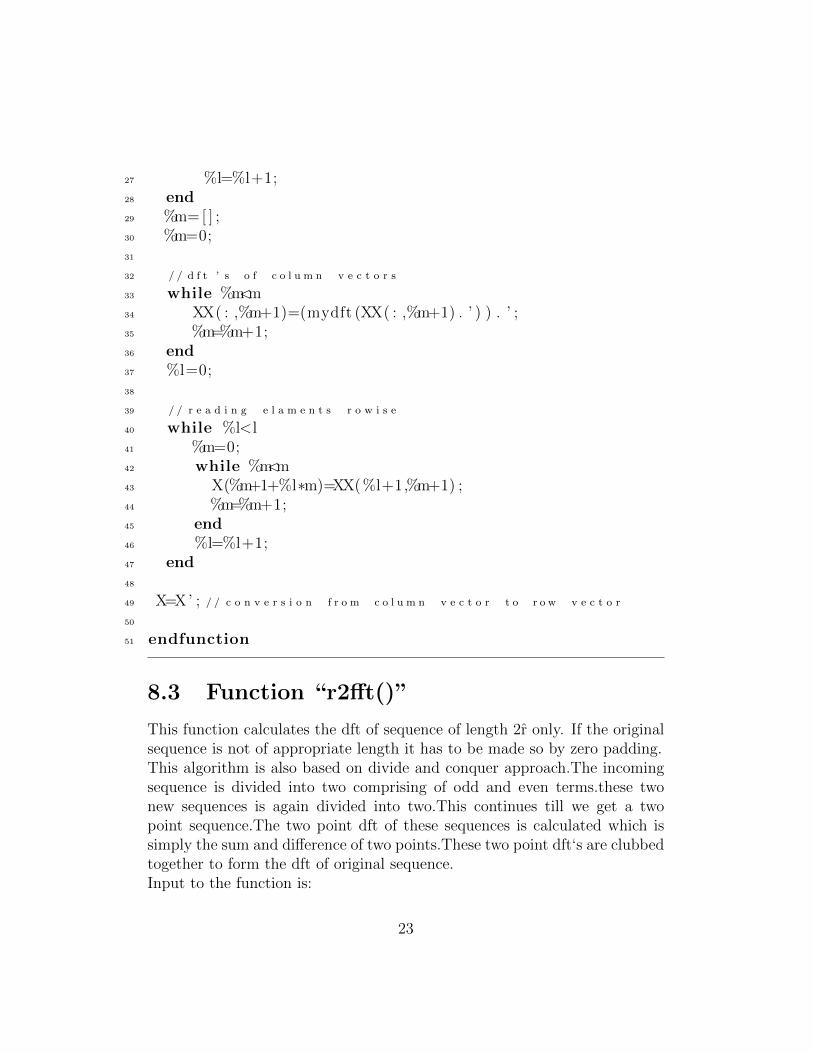
27 %l=%l+1;28 end29 %m= [ ] ;30 %m=0;31
32 / / d f t ’ s o f c o l u m n v e c t o r s
33 while %m<m34 XX( : ,%m+1)=(mydft (XX( : ,%m+1) . ’ ) ) . ’ ;35 %m=%m+1;36 end37 %l=0;38
39 / / r e a d i n g e l a m e n t s r o w i s e
40 while %l<l41 %m=0;42 while %m<m43 X(%m+1+%l∗m)=XX(%l+1,%m+1) ;44 %m=%m+1;45 end46 %l=%l+1;47 end48
49 X=X’ ; / / c o n v e r s i o n f r o m c o l u m n v e c t o r t o r o w v e c t o r
50
51 endfunction
8.3 Function “r2fft()”
This function calculates the dft of sequence of length 2r̂ only. If the originalsequence is not of appropriate length it has to be made so by zero padding.This algorithm is also based on divide and conquer approach.The incomingsequence is divided into two comprising of odd and even terms.these twonew sequences is again divided into two.This continues till we get a twopoint sequence.The two point dft of these sequences is calculated which issimply the sum and difference of two points.These two point dft‘s are clubbedtogether to form the dft of original sequence.Input to the function is:
23
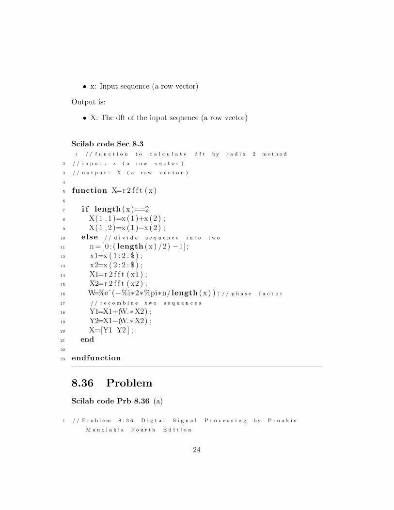
• x: Input sequence (a row vector)
Output is:
• X: The dft of the input sequence (a row vector)
Scilab code Sec 8.31 / / f u n c t i o n t o c a l c u l a t e d f t b y r a d i x 2 m e t h o d
2 / / i n p u t : x ( a r o w v e c t o r )
3 / / o u t p u t : X ( a r o w v e c t o r )
4
5 function X=r 2 f f t ( x )6
7 i f length ( x )==28 X(1 ,1 )=x (1)+x (2) ;9 X(1 ,2 )=x (1)−x (2 ) ;
10 else / / d i v i d e s e q u e n c e i n t o t w o
11 n =[0 : ( length ( x ) /2) −1];12 x1=x ( 1 : 2 : $ ) ;13 x2=x ( 2 : 2 : $ ) ;14 X1=r 2 f f t ( x1 ) ;15 X2=r 2 f f t ( x2 ) ;16 W=%eˆ(−%i∗2∗%pi∗n/ length ( x ) ) ; / / p h a s e f a c t o r
17 / / r e c o m b i n e t w o s e q u e n c e s
18 Y1=X1+(W.∗X2) ;19 Y2=X1−(W.∗X2) ;20 X=[Y1 Y2 ] ;21 end22
23 endfunction
8.36 Problem
Scilab code Prb 8.36 (a)
1 / / P r o b l e m 8 . 3 6 D i g t a l S i g n a l P r o c e s s i n g b y P r o a k i s
M a n o l a k i s F o u r t h E d i t i o n
24
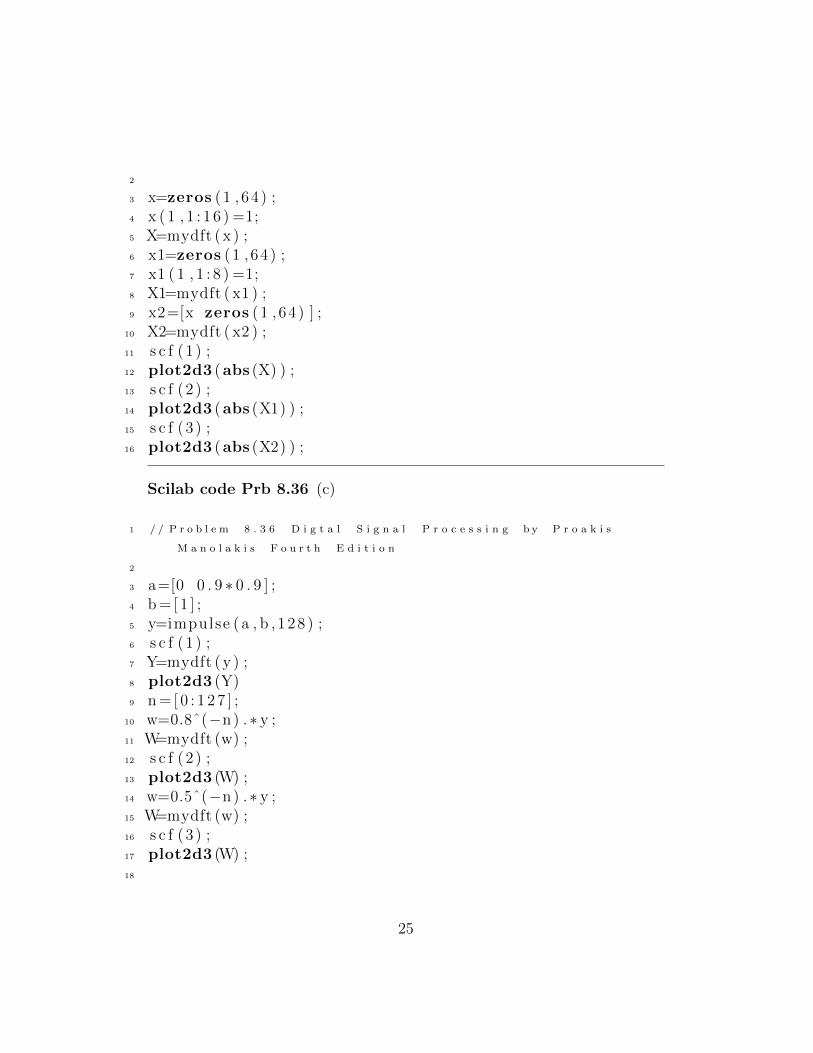
2
3 x=zeros (1 , 64 ) ;4 x ( 1 , 1 : 1 6 ) =1;5 X=mydft ( x ) ;6 x1=zeros (1 , 64 ) ;7 x1 ( 1 , 1 : 8 ) =1;8 X1=mydft ( x1 ) ;9 x2=[x zeros (1 , 64 ) ] ;
10 X2=mydft ( x2 ) ;11 s c f (1 ) ;12 plot2d3 (abs (X) ) ;13 s c f (2 ) ;14 plot2d3 (abs (X1) ) ;15 s c f (3 ) ;16 plot2d3 (abs (X2) ) ;
Scilab code Prb 8.36 (c)
1 / / P r o b l e m 8 . 3 6 D i g t a l S i g n a l P r o c e s s i n g b y P r o a k i s
M a n o l a k i s F o u r t h E d i t i o n
2
3 a=[0 0 . 9 ∗ 0 . 9 ] ;4 b = [ 1 ] ;5 y=impulse ( a , b , 128 ) ;6 s c f (1 ) ;7 Y=mydft ( y ) ;8 plot2d3 (Y)9 n = [ 0 : 1 2 7 ] ;
10 w=0.8ˆ(−n) .∗ y ;11 W=mydft (w) ;12 s c f (2 ) ;13 plot2d3 (W) ;14 w=0.5ˆ(−n) .∗ y ;15 W=mydft (w) ;16 s c f (3 ) ;17 plot2d3 (W) ;18
25

19 / / t h e d i f f e r e n c e b e t w e e n t h e t w o c u r v e s ( f i g 2 a n d f i g
3 ) i s t h a t o f a m p l i t u d e b e c a u s e p o l e i s p l a c e d m u c h
c l o s e r t o u n i t c i r c l e i n f i g 2
26
Chapter 9
Implementation of FIR and IIRfilters
In this section functions are defined to get impulse response through directform 1 implementation and to get lattice, lattice ladder coefficients fromsystem function, and vice-versa.These functions are:
• direct1(): to calculate impulse response through direct form 1 imple-mentation
• lattfir(): to get lattice coefficients of FIR filter
• lattimpilse(): to get the impulse response from lattice structure
• lattladd(): to get lattice ladder coefficients of an IIR filter
• llimpulse(): to get impulse response of an IIR through lattice ladderimplementation
9.2 Function “direct1()”, ”lattfir()” and ”lattim-
pulse()”
9.2.1 Function ”direct()”
Inputs to the function are:
27
• N: The numerator of system function (a polynomial in ’zin’ wherezin=z−1)
• D: The denominator (a polynomial in ’zin’ where zin=z−1)
• l: length of impulse response (a scalar)
Output is:
• h: The impulse response (a row vector)
Scilab code Sec 9.21 / / f u n c t i o n w h i c h t a k e s t h e s y s t e m
p o l y n o m i a l a s n u m e r a t o r a n d d e n o m i n a t o r
2 / / a n d c o m p u t e s i m p u l s e r e p o n s e b y d i r e c t f o r m 1
i m p l e m e n t a t i o n
3
4 function h=d i r e c t 1 (N,D, l )5
6 b=coeff (N) ;7 a=coeff (D) ;8 y=zeros (1 , l ) ;9 w=[b zeros (1 , l−length (b) ) ] ;
10 h (1)=w(1) ;11 index =2;12 while index<=length ( a )13 h (1 , index )=w( index )−a ( 2 : index )∗h (1 , index −1:−1:1) . ’ ;14 index=index +1;15 end16
17 while index <=l ,18 h( index )=−a ( 1 , 2 : $ )∗h (1 , $ :−1:$−length ( a )+2) . ’+w(1 ,
index ) ;19 index=index +1;20 end21
22 endfunction
28
9.2.4 Function “lattfir()”
In lattice ladder representation of FIR filters, system function Hm(z) is rep-resented as:
Hm(z) = Am(z) (9.1)
Where Am(z), by definition, is given by
Am(z) = 1 + Σαm(k)z−k (9.2)
Here m represents the degree of polynomial. Lower order polynomials in Acan be calculated using recursive formula
Am−1(z) =Am(z)−KmBm(z)
1−K2m
(9.3)
Where Km is the lattice coefficient and is equal to coefficient of z−m in Am.Bm is just the reverse polynomial of Am.Input to the function is:
• H: The system function of FIR filter (a polynomial in ’zin’ wherezin=z−1)
Output is:
• k: The lattice coefficients(a column vector)
Scilab code Sec 9.21 / / f u n c t i o n t o g e t l a t t i c e p a r a m e t e r s
f o r g i v e n f i r f i l t e r
2 / / i n p u t : H , a p o l y n o m i a l
3
4 function k=l a t t f i r (H)5
6 x=poly (0 , ”x” ) ;7 H=horner (H, x ) ; / / c o n v e r s i o n o f p o l y n o m i a l i n u n k n o w n
v a r i a b l e i n t o p o l y n o m i a l i n x
8 m=length ( coeff (H) )−1;9 A(m, 1 )=H;
10 alpha (m, : )=coeff (A(m, 1 ) ) ; / / mˆ t h r o w o f a l p h a
c o m p r i s e o f c o e f f i c i e n t s o f A m
29
11 k (m)=alpha (m,m+1) ;12 index =1;13
14 while m−index>=115 temp = [ ] ;16 temp=alpha (m−index +1,m−index +2:−1:1) ;17 B(m−index +1 ,1)=inv coeff ( temp ) ; / / c a l c B m w h i c h i s
j u s t t h e r e v e r s e p o l y n o m i a l o f A m
18 A(m−index , 1 ) =(A(m−index +1 ,1)−k (m−index +1)∗B(m−index+1 ,1) ) /(1−k (m−index +1)ˆ2) ;
19 temp1=coeff (A(m−index , 1 ) ) ;20 alpha (m−index , 1 :m−index +1)=temp1 ( 1 :m−index +1) ;21 k (m−index )=alpha (m−index ,m−index +1) ;22 index=index +1;23 end24
25 endfunction
9.3 Function ”lattimpulse()”
following are the input parameters:
• k: The lattice coefficients
It gives the following as output:
• h: The impulse reponse (a row vector)
Scilab code Sec 9.21 / / f u n c t i o n t o f i n d t h e r e s p o n s e o f
s y s t e m g i v e n l a t t i c e p a r a m e t e r s
2 function h=l a t t i m p u l s e ( k )3
4 f n (1 , 1 ) =1;5 g n (1 , 1 ) =1;6 f n 1=zeros (1 , length ( k )+1) ;7 g n 1=zeros (1 , length ( k )+1) ;8 i=1
30
9
10 while i<=length ( k )+111 index =2;12 while index<=length ( k )+113 f n (1 , index )=f n (1 , index−1)+(k ( index−1)∗ g n 1 (1 ,
index−1) ) ;14 g n (1 , index )=(k ( index−1)∗ f n (1 , index−1) )+g n 1 (1 ,
index−1) ;15 index=index +1;16 end17 h( i )=f n (1 , $ ) ;18 f n 1=f n19 g n 1=g n20 f n (1 , 1 ) =0;21 g n (1 , 1 ) =0;22 i=i +1;23 end24
25 endfunction
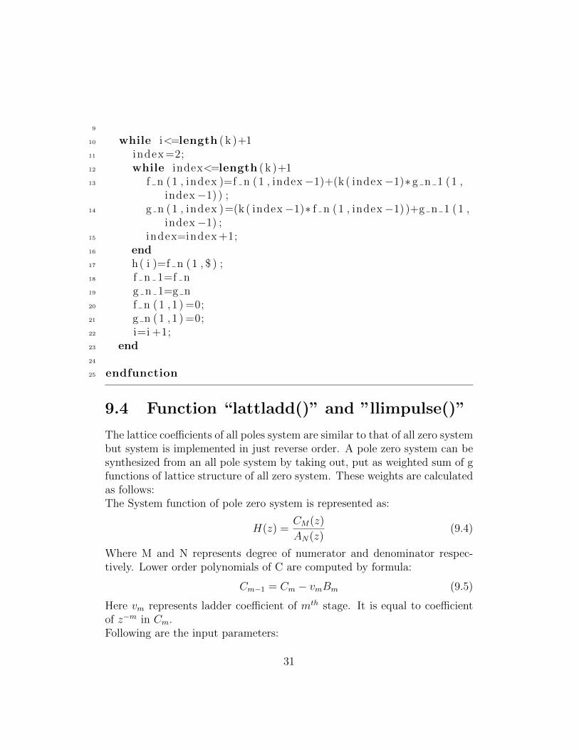
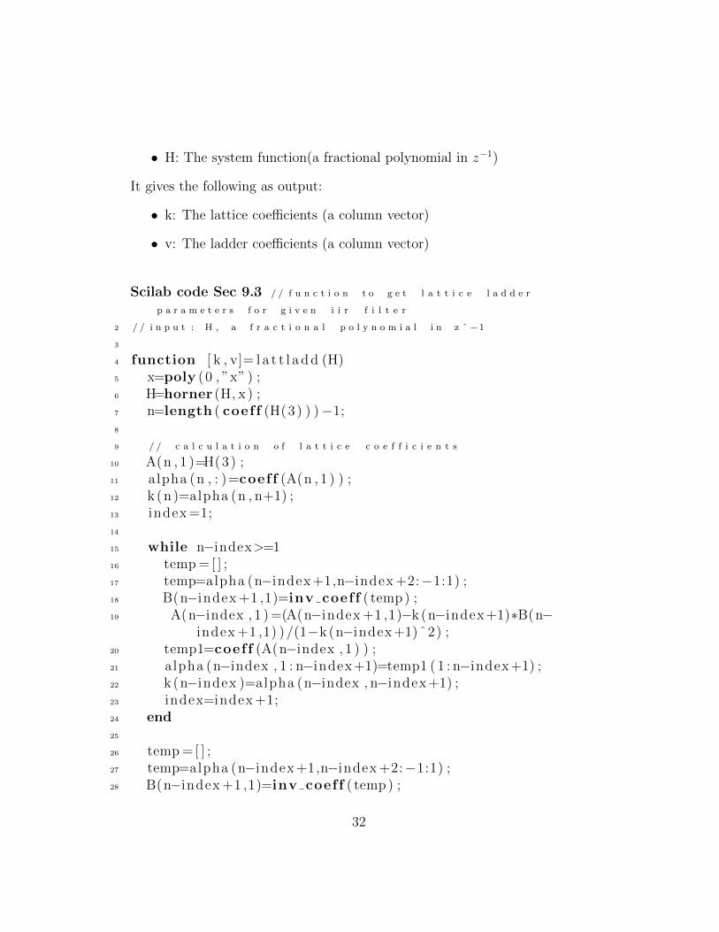
9.4 Function “lattladd()” and ”llimpulse()”
The lattice coefficients of all poles system are similar to that of all zero systembut system is implemented in just reverse order. A pole zero system can besynthesized from an all pole system by taking out, put as weighted sum of gfunctions of lattice structure of all zero system. These weights are calculatedas follows:The System function of pole zero system is represented as:
H(z) =CM(z)
AN(z)(9.4)
Where M and N represents degree of numerator and denominator respec-tively. Lower order polynomials of C are computed by formula:
Cm−1 = Cm − vmBm (9.5)
Here vm represents ladder coefficient of mth stage. It is equal to coefficientof z−m in Cm.Following are the input parameters:
31
• H: The system function(a fractional polynomial in z−1)
It gives the following as output:
• k: The lattice coefficients (a column vector)
• v: The ladder coefficients (a column vector)
Scilab code Sec 9.31 / / f u n c t i o n t o g e t l a t t i c e l a d d e r
p a r a m e t e r s f o r g i v e n i i r f i l t e r
2 / / i n p u t : H , a f r a c t i o n a l p o l y n o m i a l i n z ˆ −1
3
4 function [ k , v]= l a t t l a d d (H)5 x=poly (0 , ”x” ) ;6 H=horner (H, x ) ;7 n=length ( coeff (H(3) ) )−1;8
9 / / c a l c u l a t i o n o f l a t t i c e c o e f f i c i e n t s
10 A(n , 1 )=H(3) ;11 alpha (n , : )=coeff (A(n , 1 ) ) ;12 k (n)=alpha (n , n+1) ;13 index =1;14
15 while n−index>=116 temp = [ ] ;17 temp=alpha (n−index +1,n−index +2:−1:1) ;18 B(n−index +1 ,1)=inv coeff ( temp ) ;19 A(n−index , 1 ) =(A(n−index +1 ,1)−k (n−index +1)∗B(n−
index +1 ,1) ) /(1−k (n−index +1)ˆ2) ;20 temp1=coeff (A(n−index , 1 ) ) ;21 alpha (n−index , 1 : n−index +1)=temp1 ( 1 : n−index +1) ;22 k (n−index )=alpha (n−index , n−index +1) ;23 index=index +1;24 end25
26 temp = [ ] ;27 temp=alpha (n−index +1,n−index +2:−1:1) ;28 B(n−index +1 ,1)=inv coeff ( temp ) ;
32
29 m=length ( coeff (H(2) ) ) ;30 C(m, 1 )=H(2) ;31 gama(m, : )=coeff (C(m, 1 ) ) ;32 v (m)=gama(m,m) ;33 index =1;34
35 / / c a l c u l a t i o n o f l a d d e r c o e f f i c i e n t s
36 while m−index>=137 C(m−index , 1 )=C(m−index +1 ,1)−v (m−index +1)∗B(m−index
, 1 ) ;38 temp=coeff (C(m−index , 1 ) ) ;39 gama(m−index , 1 :m−index )=temp ( 1 :m−index ) ;40 v (m−index )=gama(m−index ,m−index ) ;41 index=index +1;42 end43
44 endfunction
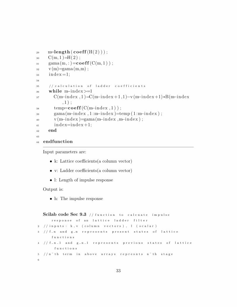
Input parameters are:
• k: Lattice coefficients(a column vector)
• v: Ladder coefficients(a column vector)
• l: Length of impulse response
Output is:
• h: The impulse response
Scilab code Sec 9.31 / / f u n c t i o n t o c a l c u a t e i m p u l s e
r e s p o n s e o f a n l a t t i c e l a d d e r f i l t e r
2 / / i n p u t s : k , v ( c o l u m n v e c t o r s ) , l ( s c a l a r )
3 / / f n a n d g n r e p r e s e n t s p r e s e n t s t a t e s o f l a t t i c e
f u n c t i o n s
4 / / f n 1 a n d g n 1 r e p r e s e n t s p r e v i o u s s t a t e s o f l a t t i c e
f u n c t i o n s
5 / / n ˆ t h t e r m i n a b o v e a r r a y s r e p r e s n t s n ˆ t h s t a g e
6
33
7 function h=l l i m p u l s e (k , v , l )8
9 N=length ( k )+110 f n (1 ,N) =1;11 f n 1 ( 1 , 1 :N) =0;12 g n (1 , 1 ) =1;13 g n 1 ( 1 , 1 :N) =0;14 i =1;15
16 while i<=l17 index =1;18 while index<N19 f n (1 ,N−index )=f n (1 ,N−index +1)−k (N−index )∗ g n 1
(1 ,N−index ) ;20 g n (1 ,N−index +1)=g n 1 (1 ,N−index )+k (N−index )∗ f n
(1 ,N−index ) ;21 index=index +1;22 end23 f n (1 ,N) =0;24 g n (1 , 1 )=f n (1 , 1 ) ;25 h( i )=g n ( 1 , 1 : length ( v ) )∗v ;26 g n 1=g n ;27 f n28 g n29 i=i +1;30 end31
32 endfunction
9.40 Problem
Scilab code Prb 9.401 / / P r o b l e m 9 . 4 0 D i g i t a l S i g n a l
P r o c e s s i n g b y P r o a k i s a n d M a n o l a k i s F o u r t h E d i t i o n
2 / / f i l e s t o b e e x e c u t e d : l a t t f i r . s c i , l a t t l a d d . s c i ,
l l i m p u l s e .
3
34
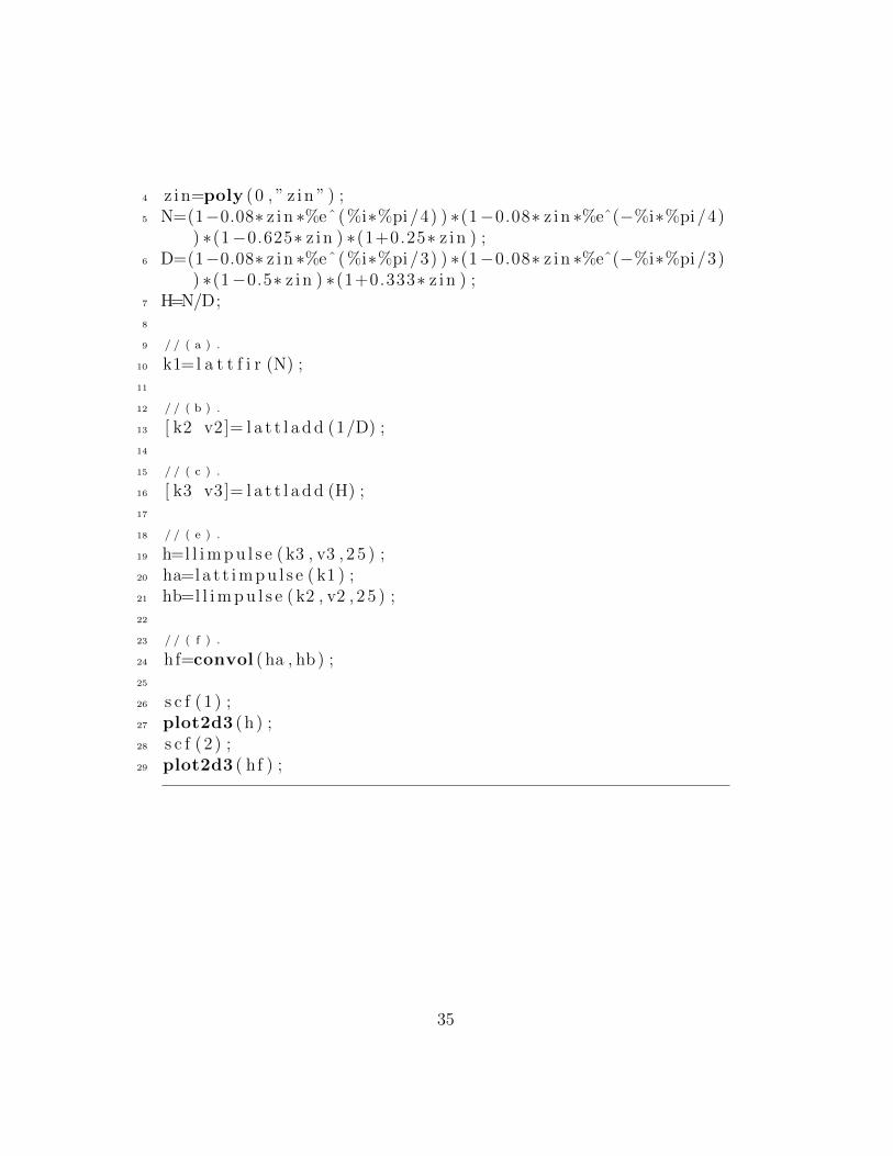
4 z in=poly (0 , ” z in ” ) ;5 N=(1−0.08∗ z in ∗%eˆ(%i∗%pi/4) ) ∗(1−0.08∗ z in ∗%eˆ(−%i∗%pi/4)
) ∗(1−0.625∗ z in ) ∗(1+0.25∗ z in ) ;6 D=(1−0.08∗ z in ∗%eˆ(%i∗%pi/3) ) ∗(1−0.08∗ z in ∗%eˆ(−%i∗%pi/3)
) ∗(1−0.5∗ z in ) ∗(1+0.333∗ z in ) ;7 H=N/D;8
9 / / ( a ) .
10 k1=l a t t f i r (N) ;11
12 / / ( b ) .
13 [ k2 v2]= l a t t l a d d (1/D) ;14
15 / / ( c ) .
16 [ k3 v3]= l a t t l a d d (H) ;17
18 / / ( e ) .
19 h=l l i m p u l s e ( k3 , v3 , 2 5 ) ;20 ha=l a t t i m p u l s e ( k1 ) ;21 hb=l l i m p u l s e ( k2 , v2 , 2 5 ) ;22
23 / / ( f ) .
24 hf=convol ( ha , hb ) ;25
26 s c f (1 ) ;27 plot2d3 (h) ;28 s c f (2 ) ;29 plot2d3 ( hf ) ;
35
Chapter 10
FIR and IIR Filter Design
10.2 FIR filter design by window method
In this section codes are presented to design FIR low-pass, high-pass,band-pass, and band-stop filters. The desired impulse response is calculated bytaking inverse fourier transform of expected spectrum. The resultant IIR isconverted into FIR by multiplying it by suitable window. The resultant FIRis made causal by shifting it by (n-1)/2 units. Where n is the length of theFIR coefficientsThe functions are:
• lpfir(): To design lowpass FIR filterInputs to the function are:
– n: Length of filter (a scalar-odd integer)
– omegac: Cut-off frequency(a scalar)
– wtype: Window type 1 for rectangle, 2 for hanning, 3 for ham-ming, 4 for blackmann
• hpfir(): To design highpass FIR filterInput to the function are:
– n: Length of filter(a scalar-odd integer)
– omegac: Cut-off frequency(a scalar)
– wtype: Window type 1 for rectangle, 2 for hanning, 3 for ham-ming, 4 for blackmann
36
• bpfir(): To design bandpass Fir filterInputs to the function are:
– n: Length of filter (a scalar-odd integer)
– omegac1: First cut-off frequency (a scalar)
– omegac2: Second cut-off frequency (a scalar)
– wtype: Window type 1 for rectangle, 2 for hanning, 3 for ham-ming, 4 for blackmann
• bsfir(): To design bandstop FIR filterInputs to the function are:
– n: Length of filter (a scalar)
– omegac1: First cut-off frequency (a scalar)
– omegac2: Second cut-off frequency (a scalar)
– wtype: Window type 1 for rectangle, 2 for hanning, 3 for ham-ming, 4 for blackmann
Scilab code Sec 10.21 / / f u n c t i o n t o g e n e r a t e l o w p a s s f i r
f i l t e r c o e f f i c i e n t s
2 / / i n p u t s : %n , o m e g c , w t y p e a l l s c a l a r s , w t y p e i n t e g e r i n
1 −4
3
4 function hc=l p f i r (%n, omegc , wtype )5
6 n = [ 1 : 1 :%n/ 2 ] ;7 hd=2∗(omegc /(2∗%pi ) )∗ sin (n∗omegc ) . / ( n∗omegc ) ;8
9 select wtype ,10 case 1 then / / r e c t a n g l e w i n d o w
11 w=ones ( 1 , (%n−1)/2) ;12 case 2 then / / h a n n i g
13 w=.5+.5∗cos (2∗%pi∗n/(%n−1) ) ;14 case 3 then / / h a mm i n g
15 w=.54+.46∗cos (2∗%pi∗n/(%n−1) ) ; ;16 case 4 then / / b l a c k m a n n
37
17 w=.42+.5∗cos (2∗%pi∗n/(%n−1) ) +.08∗cos (4∗%pi∗n/(%n−1) ) ; ;
18 end19
20 h=hd .∗w;21 hc=[h( $ :−1:1) omegc/%pi h ] ;22
23 endfunction
Scilab code Sec 10.21 / / f u n c t i o n t o g e n e r a t e h i g h p a s s f i r
f i l t e r c o e f f i c i e n t s
2 / / i n p u t s : %n , o m e g c , w t y p e a l l s c a l a r s , w t y p e i n t e g e r i n
1 −4
3
4 function hc=h p f i r (%n, omegc , wtype )5
6 n = [ 1 : 1 :%n/ 2 ] ;7 hd=−2∗(omegc /(2∗%pi ) )∗ sin (n∗omegc ) . / ( n∗omegc ) ;8
9 select wtype ,10 case 1 then / / r e c t a n g l e w i n d o w
11 w=ones ( 1 , (%n−1)/2) ;12 case 2 then / / h a n n i g
13 w=.5+.5∗cos (2∗%pi∗n/(%n−1) ) ;14 case 3 then / / h a mm i n g
15 w=.54+.46∗cos (2∗%pi∗n/(%n−1) ) ; ;16 case 4 then / / b l a c k m a n n
17 w=.42+.5∗cos (2∗%pi∗n/(%n−1) ) +.08∗cos (4∗%pi∗n/(%n−1) ) ; ;
18 end19
20 h=hd .∗w;21 hc=[h( $ :−1:1) 1−omegc/%pi h ] ;22
23 endfunction
38
Scilab code Sec 10.21 / / f u n c t i o n t o g e n e r a t e b a n d p a s s f i r
f i l t e r c o e f f i c i e n t s
2 / / i n p u t s : %n , o m e g c 1 , o m e g c 2 , w t y p e a l l s c a l a r s , w t y p e
i n t e g e r i n 1 −4
3
4 function hc=b p f i r (%n, omegc1 , omegc2 , wtype )5
6 n = [ 1 : 1 :%n/ 2 ] ;7 hd=2∗(omegc2 /(2∗%pi ) )∗ sin (n∗omegc2 ) . / ( n∗omegc2 )−2∗(
omegc1 /(2∗%pi ) )∗ sin (n∗omegc1 ) . / ( n∗omegc1 ) ;8
9 select wtype ,10 case 1 then / / r e c t a n g l e w i n d o w
11 w=ones ( 1 , (%n−1)/2) ;12 case 2 then / / h a n n i g
13 w=.5+.5∗cos (2∗%pi∗n/(%n−1) ) ;14 case 3 then / / h a mm i n g
15 w=.54+.46∗cos (2∗%pi∗n/(%n−1) ) ; ;16 case 4 then / / b l a c k m a n n
17 w=.42+.5∗cos (2∗%pi∗n/(%n−1) ) +.08∗cos (4∗%pi∗n/(%n−1) ) ; ;
18 end19
20 h=hd .∗w;21 hc=[h( $ :−1:1) ( omegc2−omegc1 ) /%pi h ] ;22
23 endfunction
Scilab code Sec 10.21 / / f u n c t i o n t o g e n e r a t e b a n d s t o p f i r
f i l t e r c o e f f i c i e n t s
2 / / I n p u t s : %n , o m e g c 1 , o m e g c 2 , w t y p e a l l s c a l a r s , w t y p e
i n t e g e r i n 1 −4
3
4 function hc=b s f i r (%n, omegc1 , omegc2 , wtype )5
6 n = [ 1 : 1 :%n/ 2 ] ;
39
7 hd=−2∗(omegc2 /(2∗%pi ) )∗ sin (n∗omegc2 ) . / ( n∗omegc2 ) +2∗(omegc1 /(2∗%pi ) )∗ sin (n∗omegc1 ) . / ( n∗omegc1 ) ;
8
9 select wtype ,10 case 1 then / / r e c t a n g l e w i n d o w
11 w=ones ( 1 , (%n−1)/2) ;12 case 2 then / / h a n n i g
13 w=.5+.5∗cos (2∗%pi∗n/(%n−1) ) ;14 case 3 then / / h a mm i n g
15 w=.54+.46∗cos (2∗%pi∗n/(%n−1) ) ; ;16 case 4 then / / b l a c k m a n n
17 w=.42+.5∗cos (2∗%pi∗n/(%n−1) ) +.08∗cos (4∗%pi∗n/(%n−1) ) ;
18 end19
20 h=hd .∗w;21 hc=[h( $ :−1:1) 1−((omegc2−omegc1 ) /%pi ) h ] ;22
23 endfunction
10.3 IIR fiter design by Butterworth filter
design and Bi-linear Transformation
Functions defined in this section are used to design Butterworth filters incontinuous time and discrete time. A Butterworth filter can be completelydefined if its pass band and stop band ripple,and its passband and stopband edge frequencies are known. First the order and cutt-off frequency offilteris calculated using these four parameters. Once these are known positionof poles in s-plane can be obtained. This completes design procedure incontinuous time. After this the digital filter can be obtained by applyingBilinear Tranformation.
The functions which are used for these purpose are:
• buttordc(): Function to calculate order of filter and its cut-off frequency
• buttord(): Function to calculate order of filter
• butterc(): Function to design analog Butterworth filter
40
• butterd(): Function to design digital Butterworth filter using BilinearTransformation.
Inputs to the function are:
• omegp: Pass band edge frequency (a scalar)
• rip pb: Pass band ripple (a scalar)
• omegs: Stopband edge frequency (a scalar)
• rip sb: Stop band ripple (a scalar)
The out put of the function are:
• n: Order of filter (a scalar-integer)
• omegc: Cut-off frequency(a scalar)
Scilab code Sec 10.31 / / B u t t e r w o r t h f i l t e r d e s i g n
2 / / f u n c t i o n t o c a l c u l a t e o r d e r a n d c u t − o f f f r e q u e n c y o f
f i l t e r
3 / / I n p u t s : om e g p , r i p p b , o m e g s , r i p s b a l l s c a l a r s
4
5 function [ n , omegc]= buttordc (omegp , r ip pb , omegs , r i p s b )6
7 Ep=(1/( r ip pb ˆ2) )−1;8 Es=(1/( r i p s b ˆ2) )−1;9 n=log ( Es/Ep) /(2∗ log ( omegs/omegp) ) ; / / o r d e r o f f i l t e r
10 n=bin2dec ( dec2bin (n) ) +1; / / a p p r o x i m a t i o n o f f i l t e r t o
i n t e g e r
11 omegc=omegs /( Es ˆ(1/(2∗n) ) ) ; / / c u t − o f f f r e q u e n c y
12
13 endfunction
Inputs to the function are:
• omegp: cut-off frequency (a scalar)
• omegs: stopband edge frequency (a scalar)
41
• rip sb: stop band ripple (a scalar)
following are the output parameters of the function
• n: order of filter (a scalar)
Scilab code Sec 10.31 / / B u t t e r w o r t h f i l t e r d e s i g n
2 / / f u n c t i o n t o c a l c u l a t e o r d e r o f f i l t e r w h e n c u t − o f f
f r e q u e n c y i s k n o w n
3 / / I n p u t : o m e g c , o m e g s , r i p s b a l l s c a l a r s
4
5 function n=buttord ( omegc , omegs , r i p s b )6
7 Es=(1/( r i p s b ˆ2) )−1;8 n=log ( Es ) /(2∗ log ( omegs/omegc ) ) ; / / o r d e r o f f i l t e r
9 n=bin2dec ( dec2bin (n) ) +1; / / a p p r o x i m a t i o n o f o r d e r t o
i n t e g e r
10
11 endfunction
Inputs to the function are:
• n: order of filter (a scalar-integer)
• omegp: cut-off frequency (a scalar-prewarped frequency)
Output is:
• G: system function in s domain (a polynomial in s)
Scilab code Sec 10.31 / / B u t t e r w o r t h f i l t e r d e s i g n
2 / / f u n c t i o n t o f i n d t r a n s f e r f u n c t i o n g i v e n t h e o r d e r
a n d c u t − o f f f r e q u e n c y
3 / / I p u t : %n , o m e g c b o t h s c a l a r s
4
5 function G=butte r c (%n, omegc )6
7 n = [ 0 : 1 :%n−1] ;
42
8 p=omegc∗%eˆ(%i∗%pi/2)∗%eˆ(%i∗%pi∗(2∗n+1)/(2∗%n) ) ; / /
p o l e s o f f i l t e r
9 a=poly (0 , ” s ” ) ;10 G=1;11 index =1;12
13 while index<=%n / / g e n e r a t i n g t h e s y s t e m f u n c t i o n
14 G=G/(a−p( index ) ) ;15 index=index +1;16 end17
18 endfunction
Inputs to the function are:
• n: order of filter (a scalar-integer)
• omegp: cut-off frequency(a scalar-prewarped frequency)
Output is:
• H: system function in Z domain (a polynomial in ’z’,in fractional form)
Scilab code Sec 10.31 / / B u t t e r w o r t h f i l t e r d e s i g n
2 / / f u n c t i o n t o f i n d t r a n s f e r f u n c t i o n g i v e n t h e o r d e r
a n d c u t − o f f f r e q u e n c y
3 / / I n p u t : %n , o m e g c b o t h s c a l a r s
4
5 function H=butterd (%n, omegc )6 n = [ 0 : 1 :%n−1] ;7 p=omegc∗%eˆ(%i∗%pi/2)∗%eˆ(%i∗%pi∗(2∗n+1)/(2∗%n) ) ; / /
p o l e s o f f i l t e r
8 a=poly (0 , ” s ” ) ;9 G=1;
10 index =1;11
12 while index<=%n / / g e n e r a t i n g s y s t e m f u n c t i o n
13 G=G/(a−p( index ) ) ;14 index=index +1;
43

15 end16
17 b=poly (0 , ”z” ) ;18 s =(2) ∗(b−1)/(b+1) ; / / b i l i n e a r t r a n s f o r m a t i o n
19 H=horner (G, s ) ;20
21 endfunction
44
Solved examples from book’sappendix
Scilab code Exa 16 Example 16, page no. 1098
1 / / E x a m p l e P r o b l e m n o . 1 6
2
3 fp =250;4 f s =1000;5 omegp=2∗%pi∗ fp / f s ;6 hr=l p f i r (11 , omegp , 1 )7 hhan=l p f i r (11 , omegp , 2 )8 hham=l p f i r (11 , omegp , 3 )9 hblack=l p f i r (11 , omegp , 4 )
Scilab code Exa 17 Example 17, page no. 1103
1 / / E x a m p l e P r o b l e m n o . 1 7
2
3 f c =250;4 f s =1000;5 omegp=2∗%pi∗ fp / f s ;6 hr=h p f i r (7 , omegp , 1 )7 hhan=h p f i r (7 , omegp , 2 )8 hham=h p f i r (7 , omegp , 3 )9 hblack=h p f i r (7 , omegp , 4 )
Scilab code Exa 18 Example 18, page no. 1104
45
1 / / E x a m p l e P r o b l e m n o . 1 8
2
3 f c 1 =100;4 f c 2 =200;5 f s =1000;6 omegc1=2∗%pi∗ f c 1 / f s ;7 omegc2=2∗%pi∗ f c 2 / f s ;8 hr=b p f i r (9 , omegc1 , omegc2 , 1 )9 hhan=b p f i r (9 , omegc1 , omegc2 , 2 )
10 hham=b p f i r (9 , omegc1 , omegc2 , 3 )11 hblack=b p f i r (9 , omegc1 , omegc2 , 4 )
Scilab code Exa 25 Example 25, page no. 1114
1 / / S o l v e d E x a m p l e No . 2 5 D i g i t a l S i g n a l P r o c e s s i n g
P r o a k i s M a n o l a k i s F o u r t h E d i t i o n
2 / / F i l e s t o b e e x e c u t e d : b u t t o r d c . s c e , b u t t e r d . s c e
3
4 r ip pb =10ˆ(−1.25/20) ;5 r i p s b =10ˆ(−15/20) ;6 fpb =200;7 f s b =300;8 f s =2000;9 omegs=2∗%pi∗ f s b / f s ;
10 omegp=2∗%pi∗ fpb / f s ;11 omegs pw=2∗tan ( omegs /2) ; / / p r e w a r p e d f r e q u e n c y
12 omegp pw=2∗tan ( omegp/2) ; / / p r e w a r p e d f r e q u e n c y
13 [ n , omegc]= buttordc (omegp pw , r ip pb , omegs pw , r i p s b ) ; / /
o r d e r a n d c u t − o f f f r e q u e n c y
14 sys fun=butterd (n , omegc ) / / d i g i t a l s y s t e m
Scilab code Exa 25 Example 29, page no. 1120
1 / / S o l v e d E x a m p l e No . 2 9 D i g i t a l S i g n a l P r o c e s s i n g b y
P r o a k i s M a n o l a k i s F o u r t h E d i t i o n
2 / / F i l e t o b e e x e c u t e d : b u t t e r c . s c e
3
4 f l =200;
46
5 fu =300;6 f s =1000;7 omegl=2∗%pi∗ f l / f s ;8 omegu=2∗ fu ∗%pi/ f s ;9 omegl pw=2∗tan ( omegl /2) ; / / p r e w r p e d f r e q u e n c y
10 omegu pw=2∗tan ( omegu/2) ; / / p r e w r p e d f r e q u e n c y
11 G=butte r c ( 1 , 1 , 1 ) ; / / a n a l o g l o w p a s s f i l t e r w i t h c u t − o f f
1 o r d e r 1
12 a=poly (0 , ” s ” ) ;13 s=(aˆ2+(omegu pw∗omegl pw ) ) /( a∗(omegu pw−omegl pw ) ) ; / /
T r a n s f o r m a t i o n
14 G=horner (G, s ) / / a n a l o g b a n d − p a s s f i l t e r
47


![[John Proakis] Digital Communications(BookFi.org)](https://img.pdfslide.us/doc/110x75/56d6be9d1a28ab301692e190/john-proakis-digital-communicationsbookfiorg-570f113ed1824.jpg)