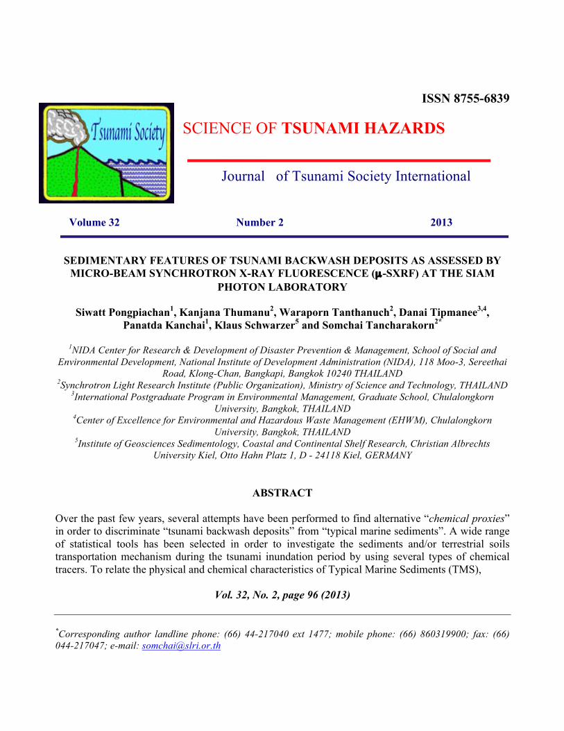
ISSN 8755-6839

SCIENCE OF TSUNAMI HAZARDS

Journal of Tsunami Society International

Volume 32 Number 2 2013

SEDIMENTARY FEATURES OF TSUNAMI BACKWASH DEPOSITS AS ASSESSED BY

MICRO-BEAM SYNCHROTRON X-RAY FLUORESCENCE (µ-SXRF) AT THE SIAM PHOTON LABORATORY

Siwatt Pongpiachan1, Kanjana Thumanu2, Waraporn Tanthanuch2, Danai Tipmanee3,4,

Panatda Kanchai1, Klaus Schwarzer5 and Somchai Tancharakorn2*

1NIDA Center for Research & Development of Disaster Prevention & Management, School of Social and Environmental Development, National Institute of Development Administration (NIDA), 118 Moo-3, Sereethai

Road, Klong-Chan, Bangkapi, Bangkok 10240 THAILAND 2Synchrotron Light Research Institute (Public Organization), Ministry of Science and Technology, THAILAND

3International Postgraduate Program in Environmental Management, Graduate School, Chulalongkorn University, Bangkok, THAILAND

4Center of Excellence for Environmental and Hazardous Waste Management (EHWM), Chulalongkorn University, Bangkok, THAILAND

5Institute of Geosciences Sedimentology, Coastal and Continental Shelf Research, Christian Albrechts University Kiel, Otto Hahn Platz 1, D - 24118 Kiel, GERMANY

ABSTRACT Over the past few years, several attempts have been performed to find alternative “chemical proxies” in order to discriminate “tsunami backwash deposits” from “typical marine sediments”. A wide range of statistical tools has been selected in order to investigate the sediments and/or terrestrial soils transportation mechanism during the tsunami inundation period by using several types of chemical tracers. To relate the physical and chemical characteristics of Typical Marine Sediments (TMS),

Vol. 32, No. 2, page 96 (2013)

*Corresponding author landline phone: (66) 44-217040 ext 1477; mobile phone: (66) 860319900; fax: (66) 044-217047; e-mail: somchai@slri.or.th

Tsunami Backwash Deposits (TBD), Onshore Tsunami Deposits (OTD) and Coastal Zone Soils (CZS) with their synchrotron radiation based micro-X-ray Fluorescence (µ-SXRF) spectra, the µ-SXRF spectra were built in the appropriate selected spectra range from 3,000 eV to 8,000 eV. Further challenges were considered by using the first-order derivative µ-SXRF spectra coupled with Probability Distribution Function (PDF), Hierarchical Cluster Analysis (HCA) and Principal Component Analysis (PCA) in order to investigate the elemental distribution characteristics in various types of terrestrial soils and marine sediments. Dendrographic classifications and multi-dimensional plots of principal components (i.e. bi-polar and three dimensional plots) could indicate the impacts of terrestrial soils and/or marine sediments transport on onshore and/or offshore during the tsunami inundation period. Obviously, these advanced statistical analyses are quite useful and provide valuable information and thus shed new light on the study of paleotsunami. Keywords: Andaman Sea; Tsunami Backwash Deposits; Micro-beam Synchrotron X-ray Fluorescence (µ-SXRF); First Order Derivative; Hierarchical Cluster Analysis; Principal Component Analysis. 1. INTRODUCTION The 2004 Sumatra-Andaman earthquake and tsunami was commonly considered as the worst natural disaster to ever attack Southeast Asian countries, triggering death and injury as well as major destruction to the transportation system, property, and environmental and economic sustainability (Griffin et al., 2013; Matsumaru et al., 2012). The severe impact on the beach zone between the Pakarang Cape and the Khao Lak, Phang-nga province of Thailand in turn had serious consequences on the scoured features existed in both on the beach side and in the embayment of tidal channels (Choowong et al., 2007, 2009; Fagherazzi and Du, 2007). In spite of various papers focusing on geomorphological, sedimentological and geological alterations in tsunami-affected areas (Choowong et al., 2007, 2008a, 2008b, 2009;Szczuciński et al., 2005, 2006, 2007), the knowledge of chemical distribution is strictly limited. As a consequence, several challenges have been made to conduct both qualitative and quantitative analyses of various chemical species in both onshore and offshore of tsunami-affected regions (Goff et al., 2012; Jagodziński et al., 2012; Pongpiachan et al., 2012; Pongpiachan et al., 2013; Sakuna et al., 2012; Tipmanee et al., 2012). In order to understand the destructive behaviour of tsunami affecting both onshore and offshore areas, numerous studies have attempted to draw the scientific community’s attention on the feasibility of chemical tracers to characterize tsunami backwash deposits from those of typical marine sediments (Pongpiachan et al., 2012; Pongpiachan et al., 2013; Tipmanee et al., 2012). Since the identification of tsunami backwash deposit is the first step to gain information on tsunami impacts, it is therefore essentially crucial to find an alternative method to discriminate tsunami backwash deposits from those of natural background submarine sediments. In the past few years, X-ray fluorescence (XRF) have been widely used for the determination of

Vol. 32, No. 2, page 97 (2013)

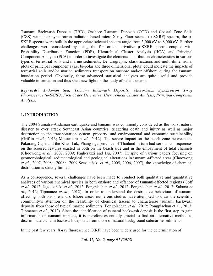
elements in sedimentological record of tsunamis on the Portuguese Shelf off Lisbon (Abrantes et al., 2008), geoarchaeological evidence of multiple tsunamigenic imprint on the Bay of Palairos-Pogonia, Greece (Vött et al., 2011)) and most recently sedimentary deposits left by the 2004 Indian Ocean tsunami on the inner continental shelf offshore of Khao Lak, Andaman Sea, Thailand (Sakuna et al., 2011). XRF has gained more popularity on studies of environmental sciences because of its relatively low cost solution compared to other analytical instruments, non-destructive testing solution, fast processing time, typical detection limit of around 0.01% for most elements and quantitative analysis. Recently, the shared use of synchrotron radiation based micro-X-ray Fluorescence (µ-SXRF) permits analysis of objects at the micron-scale owing to its high intensity and energy tenability in comparison with those of conventional light sources such as sealed-tube or rotating-anode generators (Tancharakorn et al., 2012). Because of micrometer sized X-ray beam, one can use µ-SXRF not only to quantify the elemental compositions in target samples but also its distribution at the micrometer scale (Kanngieβer & Haschke, 2006). In this research, the author postulates that the use of µ-SXRF in cooperation with the first derivative, probability distribution functions (PDF), hierarchical cluster analysis (HCA) and principal component analysis (PCA) provides a better insight of sedimentary features of tsunami backwash deposits in comparison with those of typical marine sediments and terrestrial components. Note that this is the first time to employ µ-SXRF with assistance of synchrotron radiation in order to assess the elemental distribution of tsunami backwash deposits in micro-scale. It is also worth mentioning that neither the source apportionment, nor the analysis of spatial variation of chemical components in sediments is the principal objective of this paper. 2. MATERIALS & METHODS 2.1 Sampling sites & sampling procedure 2.1.1 Surface marine sediment The research area is governed by two seasonal monsoons: the northeast monsoon from mid October until March and the southwest monsoon from May to September. This study was carried out offshore along the west coast of Phang Nga province, in the southwest region of Thailand, which was heavily affected by the 2004 tsunami. The research area covers approximately 1,000 km2 between Thap Lamu and Pakarang Cape, up to a water depth of 70 meters. Our research was carried out on research cruises taken from one year apart, from November-December 2007 with RV CHAKRATONG TONGYAI and November-December 2008 with RV BOONLERT PASOOK, covering approximately 1500 nautical miles of hydroacoustic profiles (side scan sonar, multibeam echo sounder and shallow reflection seismic with a boomer system) were recorded at Pakarang Cape. Twenty of sediment samples were collected during 18-20 July 2009 (Fig. 1)). The sampling stations were selected on the basis of the basic data acquired from hydroacoustic mapping using equipment, which consisted of Multi-beam, Side Scan Sonar and Boomer system to investigate the sedimentary deposition on near-

Vol. 32, No. 2, page 98 (2013)

shore seabed (Feldens et al., 2009; Feldens et al., 2012). These supporting data provided the geophysical structure of seabed, which was promising evidence of terrestrial deposits in the study area. Van-veen Grab Sampler was used to collect the 20 surface sediment samples. Sediment samples were wrapped in clean aluminum foil, placed in a glass bottle, and kept frozen at – 20 ºC.

Fig. 1: Sampling site description at tsunami affected area at Khao Lak, Phang-nga province of

Thailand.

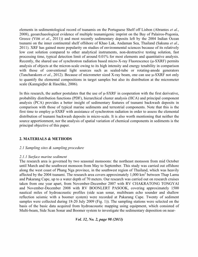
2.1.2 Terrestrial soils Ten of terrestrial soil samples were collected during 18-20 July 2009. Soil sampling stations were selected by considering the areas, which were affected by the 2004 Tsunami (Szczucinski et al., 2005). In addition, the locations of soil sampling stations were also in the transect line of the surface sediment sampling stations (Fig.1-2). They were collected during 18-20 July 2009. The surface layer was collected by using a clean shovel. About half kilogram of composite samples from 2 m2 area of each station was taken (Badin et al., 2008). They were wrapped in clean aluminum foil, placed in a glass bottle, and kept frozen at - 20ºC

Vol. 32, No. 2, page 99 (2013)

Fig. 2: Tsunami and Post-tsunami deposition layer at Khao Lak, Phang-nga province of Thailand.

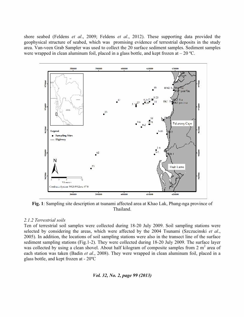
2.2 Sample preparation for µ-SXRF Due to the heterogeneity of sediment, all samples for XRF measurement were prepared in homogenous and flat discs using grinding and pelletizing processes. In the grinding process, 100 g of powder was weighted and put into a 10 ml ZrO2 grinding bowl with two ZrO2 balls (Ø 10 mm) and seven SiO2 balls (Ø 5 mm) and shaken at 1,800 oscillations/min for 30 minutes (Fig. 3). Then, in the pelletizing process, 50 g of homogenous powder was put into a steel mould and pressurized at 4 tons for 1 minute to form a 13 mm in diameter disc.

Vol. 32, No. 2, page 100 (2013)

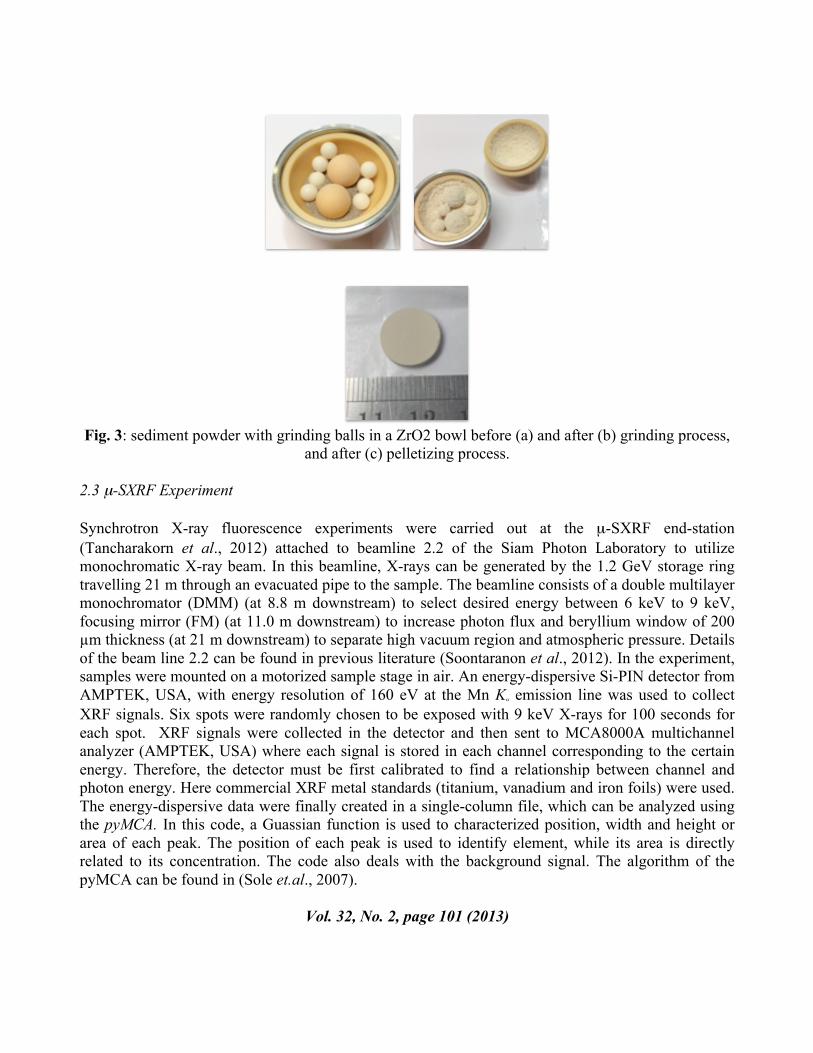
Fig. 3: sediment powder with grinding balls in a ZrO2 bowl before (a) and after (b) grinding process,

and after (c) pelletizing process. 2.3 µ-SXRF Experiment Synchrotron X-ray fluorescence experiments were carried out at the µ-SXRF end-station (Tancharakorn et al., 2012) attached to beamline 2.2 of the Siam Photon Laboratory to utilize monochromatic X-ray beam. In this beamline, X-rays can be generated by the 1.2 GeV storage ring travelling 21 m through an evacuated pipe to the sample. The beamline consists of a double multilayer monochromator (DMM) (at 8.8 m downstream) to select desired energy between 6 keV to 9 keV, focusing mirror (FM) (at 11.0 m downstream) to increase photon flux and beryllium window of 200 µm thickness (at 21 m downstream) to separate high vacuum region and atmospheric pressure. Details of the beam line 2.2 can be found in previous literature (Soontaranon et al., 2012). In the experiment, samples were mounted on a motorized sample stage in air. An energy-dispersive Si-PIN detector from AMPTEK, USA, with energy resolution of 160 eV at the Mn Kα emission line was used to collect XRF signals. Six spots were randomly chosen to be exposed with 9 keV X-rays for 100 seconds for each spot. XRF signals were collected in the detector and then sent to MCA8000A multichannel analyzer (AMPTEK, USA) where each signal is stored in each channel corresponding to the certain energy. Therefore, the detector must be first calibrated to find a relationship between channel and photon energy. Here commercial XRF metal standards (titanium, vanadium and iron foils) were used. The energy-dispersive data were finally created in a single-column file, which can be analyzed using the pyMCA. In this code, a Guassian function is used to characterized position, width and height or area of each peak. The position of each peak is used to identify element, while its area is directly related to its concentration. The code also deals with the background signal. The algorithm of the pyMCA can be found in (Sole et.al., 2007).

Vol. 32, No. 2, page 101 (2013)

2.4 Statistical analysis The derivative spectrophotometric method is based on transformation of zero-order spectra of sediment and soil samples into the first-order derivative (ΔPhoton Energy (eV)/ΔIntensity (counts)). In this study, the value of first derivative was performed by using the Software OPUS Version 7.0. In addition, first derivatives of the spectral data from each sampling location were treated through hierarchical cluster analysis (HCA) and principal component analysis (PCA) with the orthogonal Varimax solution using Statistical Package for the Social Sciences (SPSS) Version 13.0. 3. RESULTS & DISCUSSION 3.1.Characteristics of the first-order derivative µ-SXRF spectra Although several attempts have been made by several researchers to quantify chemical contents in sediments in order to elucidate tsunami backwash mechanism (Pongpiachan et al., 2012; Pongpiachan et al., 2013; Sakuna et al., 2012; Tipmanee et al., 2012;), some alternative proxies are always required to enhance the reliability of data interpretation. In this study, the assessment of µ-SXRF spectra as an alternative “fingerprint” to discriminate tsunami backwash deposit from typical marine sediments was performed by using the concept of first derivative. All samples were classified into four groups namely “Typical Marine Sediments (TMS)”, “Tsunami Backwash Deposits (TBD)”, “Onshore Tsunami Deposits (OTD)” and “Coastal Zone Terrestrial Soils (CTS)” as clearly described in Table 1.

Table 1. Sample information of marine sediments and terrestrial soils.

Sampling code Sampling date Sampling description Coastal Zone Soils (CZS) Tub1 July-18-2009 Canal bank PK 3 July-19-2009 Shrimp pond BN 2 July-20-2009 Canal bank BP 3 July-20-2009 Mangrove

Onshore Tsunami Deposits (OTD)

BK 1 Post Tsu, BK1 Tsu July-19-2009 Tsunami deposit layer BK 5 Tsu July-19-2009 Tsunami deposit layer BM 1 Tsu July-20-2009 Tsunami deposit layer BM 2 Post Tsu, BM2 Tsu July-20-2009 Pond

Vol. 32, No. 2, page 102 (2013)

Typical Marine Sediments (TMS)

10, 17 December-1-2007 Pakarang cape sediment 3-2 ,3-6, 3-16, 4-2, 4-6, 5-20, 5-25 March-4-5- 2010 Pakarang cape sediment 53, 62 December-7-2007 Thup Lamu Sediment

Tsunami Backwash Deposits (TBD) 23, 27, 31, 39, 72, 78 December-3-2007 Tsunami affected sediment 5-17, 5-21, 5-23 March-5- 2010 Tsunami affected sediment The average µ-SXRF spectra of four sample groups are compared and carefully investigated (See Fig. 4). Generally, all sample groups display similar spectral characteristics. There are four prominent features, which are common to all µ-SXRF spectra: a) main element which can be found in all samples is calcium (Kα at 3.69 keV, Kβ at 4.01 keV); b) all samples have a relatively small amount of titanium (Kα at 4.51 keV, Kβ at 4.93 keV) and manganese (Kα at 5.90 keV, Kβ at 6.49 keV); c) another main element contained in all samples is iron(Kα at 6.40 keV, Kβ at 7.06 keV); and d) low concentration of three elements which are potassium ((Kα at 3.31 keV, Kβ at 3.59 keV), titanium and manganese were detected in OTD samples. Based on these results, one can deduce that all elemental species in samples share comparable distribution patterns.

Fig. 4: µ-SXRF spectra of typical marine sediments (TMS), tsunami backwash deposits (TBD), on-

shore tsunami deposits (OTD) and coastal zone soils (CZS).

Vol. 32, No. 2, page 103 (2013)

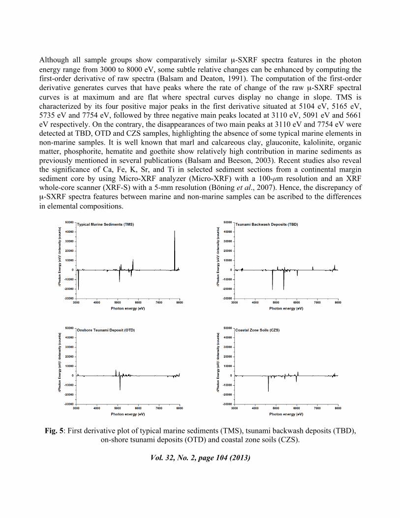
Although all sample groups show comparatively similar µ-SXRF spectra features in the photon energy range from 3000 to 8000 eV, some subtle relative changes can be enhanced by computing the first-order derivative of raw spectra (Balsam and Deaton, 1991). The computation of the first-order derivative generates curves that have peaks where the rate of change of the raw µ-SXRF spectral curves is at maximum and are flat where spectral curves display no change in slope. TMS is characterized by its four positive major peaks in the first derivative situated at 5104 eV, 5165 eV, 5735 eV and 7754 eV, followed by three negative main peaks located at 3110 eV, 5091 eV and 5661 eV respectively. On the contrary, the disappearances of two main peaks at 3110 eV and 7754 eV were detected at TBD, OTD and CZS samples, highlighting the absence of some typical marine elements in non-marine samples. It is well known that marl and calcareous clay, glauconite, kalolinite, organic matter, phosphorite, hematite and goethite show relatively high contribution in marine sediments as previously mentioned in several publications (Balsam and Beeson, 2003). Recent studies also reveal the significance of Ca, Fe, K, Sr, and Ti in selected sediment sections from a continental margin sediment core by using Micro-XRF analyzer (Micro-XRF) with a 100-µm resolution and an XRF whole-core scanner (XRF-S) with a 5-mm resolution (Böning et al., 2007). Hence, the discrepancy of µ-SXRF spectra features between marine and non-marine samples can be ascribed to the differences in elemental compositions.

Fig. 5: First derivative plot of typical marine sediments (TMS), tsunami backwash deposits (TBD),

on-shore tsunami deposits (OTD) and coastal zone soils (CZS).

Vol. 32, No. 2, page 104 (2013)

3.2 Probability distribution function (PDF) In probability theory, a probability density function (PDF) is a function that defines the comparative possibility for this random variable to take on a certain value. The probability for the random variable to fall within a particular region is given by the integral of this variable’s density over the region. The probability density function is nonnegative everywhere, and its integral over the entire space is equal to one. PDF was employed to all µ-SXRF spectra in the intensity range from 0 to 400 counts as clearly displayed in Fig. 6. Generally, the probability density of standard normal distribution can be described as follows:

(1)

where e, x and π represent for exponential constant (i.e. 2.718), intensity (counts) and pi value (i.e. 3.142) respectively. If a random variable X is provided and its distribution possesses a probability density function f, then the estimated value of X can be computed as

(2)

A distribution has a density function if and only if its cumulative distribution function F(x) is absolutely continuous. In this case: F is almost everywhere differentiable, and its derivative can be used as probability density:

(3)

PDF is a function that describes the relative likelihood for this random variable to take on a given value. The probability for the random variable to fall within a particular region is given by the Gaussian distribution, which can be described as follows:

(4)

where y, σ, σ2, µ and x represent for probability distribution function (PDF), standard deviation of µ-SXRF spectra intensity, variance of µ-SXRF spectra intensity, average of µ-SXRF spectra intensity and µ-SXRF spectra intensity of all samples respectively.

Vol. 32, No. 2, page 105 (2013)

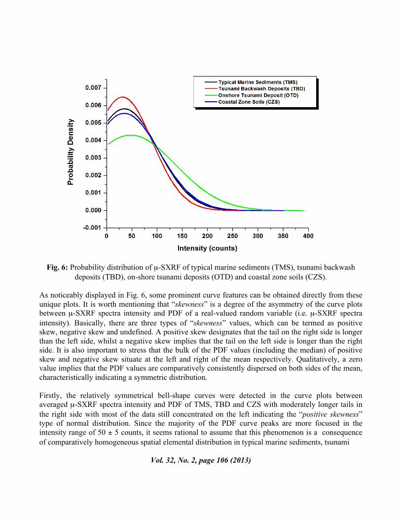
Fig. 6: Probability distribution of µ-SXRF of typical marine sediments (TMS), tsunami backwash

deposits (TBD), on-shore tsunami deposits (OTD) and coastal zone soils (CZS). As noticeably displayed in Fig. 6, some prominent curve features can be obtained directly from these unique plots. It is worth mentioning that “skewness” is a degree of the asymmetry of the curve plots between µ-SXRF spectra intensity and PDF of a real-valued random variable (i.e. µ-SXRF spectra intensity). Basically, there are three types of “skewness” values, which can be termed as positive skew, negative skew and undefined. A positive skew designates that the tail on the right side is longer than the left side, whilst a negative skew implies that the tail on the left side is longer than the right side. It is also important to stress that the bulk of the PDF values (including the median) of positive skew and negative skew situate at the left and right of the mean respectively. Qualitatively, a zero value implies that the PDF values are comparatively consistently dispersed on both sides of the mean, characteristically indicating a symmetric distribution. Firstly, the relatively symmetrical bell-shape curves were detected in the curve plots between averaged µ-SXRF spectra intensity and PDF of TMS, TBD and CZS with moderately longer tails in the right side with most of the data still concentrated on the left indicating the “positive skewness” type of normal distribution. Since the majority of the PDF curve peaks are more focused in the intensity range of 50 ± 5 counts, it seems rational to assume that this phenomenon is a consequence of comparatively homogeneous spatial elemental distribution in typical marine sediments, tsunami

Vol. 32, No. 2, page 106 (2013)

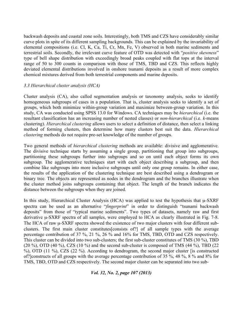
backwash deposits and coastal zone soils. Interestingly, both TMS and CZS have considerably similar curve plots in spite of its different sampling backgrounds. This can be explained by the invariability of elemental compositions (i.e. Cl, K, Ca, Ti, Cr, Mn, Fe, V) observed in both marine sediments and terrestrial soils. Secondly, the irrelevant curve feature of OTD was detected with “positive skewness” type of bell shape distribution with exceedingly broad peaks coupled with flat tops at the interval range of 50 to 300 counts in comparison with those of TMS, TBD and CZS. This reflects highly deviated elemental distributions involved in onshore tsunami deposits as a result of more complex chemical mixtures derived from both terrestrial components and marine deposits. 3.3 Hierarchical cluster analysis (HCA) Cluster analysis (CA), also called segmentation analysis or taxonomy analysis, seeks to identify homogeneous subgroups of cases in a population. That is, cluster analysis seeks to identify a set of groups, which both minimize within-group variation and maximize between-group variation. In this study, CA was conducted using SPSS 13.0 for Windows. CA techniques may be hierarchical (i.e. the resultant classification has an increasing number of nested classes) or non-hierarchical (i.e. k-means clustering). Hierarchical clustering allows users to select a definition of distance, then select a linking method of forming clusters, then determine how many clusters best suit the data. Hierarchical clustering methods do not require pre-set knowledge of the number of groups. Two general methods of hierarchical clustering methods are available: divisive and agglomerative. The divisive technique starts by assuming a single group, partitioning that group into subgroups, partitioning these subgroups further into subgroups and so on until each object forms its own subgroup. The agglomerative techniques start with each object describing a subgroup, and then combine like subgroups into more inclusive subgroups until only one group remains. In either case, the results of the application of the clustering technique are best described using a dendrogram or binary tree. The objects are represented as nodes in the dendrogram and the branches illustrate when the cluster method joins subgroups containing that object. The length of the branch indicates the distance between the subgroups when they are joined. In this study, Hierarchical Cluster Analysis (HCA) was applied to test the hypothesis that µ-SXRF spectra can be used as an alternative “fingerprint” in order to distinguish “tsunami backwash deposits” from those of “typical marine sediments”. Two types of datasets, namely raw and first derivative µ-SXRF spectra of all samples, were employed to HCA as clearly illustrated in Fig. 7-8. The HCA of raw µ-SXRF spectra showed the existence of two major clusters with four different sub-clusters. The first main cluster constitutes[consists of?] of all sample types with the average percentage contribution of 37 %, 21 %, 26 % and 16% for TMS, TBD, OTD and CZS respectively. This cluster can be divided into two sub-clusters; the first sub-cluster constitutes of TMS (30 %), TBD (20 %), OTD (40 %), CZS (10 %) and the second sub-cluster is composed of TMS (44 %), TBD (22 %), OTD (11 %), CZS (22 %). According to dendrogram, the second major cluster [is constructed of?]constructs of all groups with the average percentage contribution of 35 %, 48 %, 8 % and 8% for TMS, TBD, OTD and CZS respectively. The second major cluster can be separated into two sub-

Vol. 32, No. 2, page 107 (2013)

clusters; the third sub-cluster [is comprised of?]comprises of TMS (20 %), TBD (80 %), OTD (0 %), CZS (0 %) and the fourth sub-cluster is composed of TMS (35 %), TBD (48 %), OTD (8 %), CZS (8 %). The second major cluster can be considered as a mixture of “typical marine sediments” and “tsunami backwash deposits”, which has been highly characterized in the third sub-cluster (See Fig. 7).

Fig. 7: Dendrographic classification with raw data of typical marine sediments (TMS), tsunami backwash deposits (TBD), on-shore tsunami deposits (OTD) and coastal zone soils (CZS). The

Euclidean distance after vector normalization spectra and the Ward linkage method were employed. For details about cluster group composition see data in Table 1.

Vol. 32, No. 2, page 108 (2013)

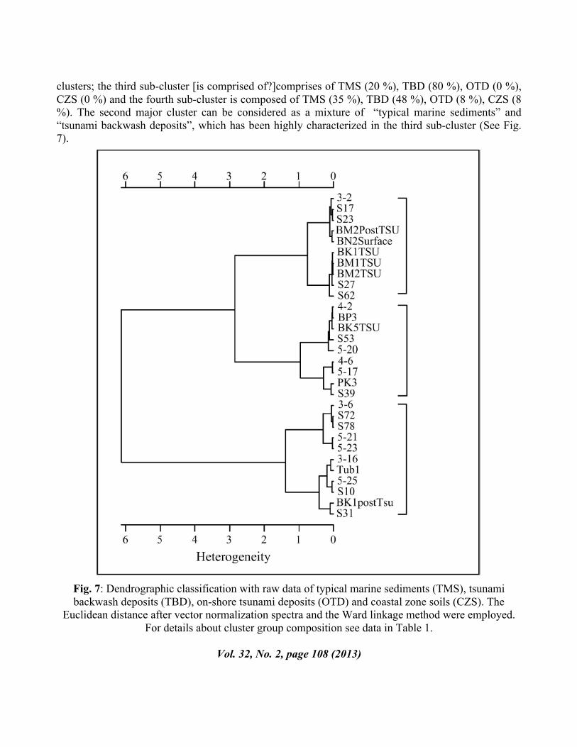
Further efforts to underline the importance of µ-SXRF spectra as an alternative “fingerprint” have been conducted by using the first derivative data. It can be seen in Fig. 8 that the OTD samples are highly deviated from CZS samples, which emphasizes the strong discrepancy in elemental distribution between onshore tsunami deposits and coastal zone soils. Interestingly, TMS samples have a high degree of similarity with those of OTD samples. This particular phenomenon can be ascribed as heavily influenced by advancement of large-scale tsunami inundation, which is responsible for extensive sediment transport from the offshore and subsequently deposited over the coastal areas. Similarly, TBD samples share a high level of affinity with those of CZS samples. This unique occurrence can be attributed to rapid tsunami backwash, which carried terrestrial debris from the onshore to the offshore.

Fig. 8: Dendrographic classification with the first-order derivative data of typical marine sediments (TMS), tsunami backwash deposits (TBD), on-shore tsunami deposits (OTD) and coastal zone soils (CZS). The Euclidean distance after vector normalization spectra and the Ward linkage method were

employed. For details about cluster group composition see data in Table 1.

Vol. 32, No. 2, page 109 (2013)

3.4 Principal component analysis (PCA) In PCA, all variables are expressed in standardized form with a mean of 0 and a standard deviation of 1. The total variance therefore equals the total number of variables, and the variance of each factor expressed as a fraction of the total variance is referred to as the eigenvalue. If a factor has a low eigenvalue, then it is contributing little to the explanation of variances in the variables and may be ignored. PCA is generally used when the research purpose is data reduction (i.e. to reduce the information in many measured variables into a smaller set of components). PCA seeks a linear combination of variables such that the maximum variance is extracted from the variables. It then removes this variance and seeks a second linear combination that explains the maximum proportion of the remaining variance, and so on. This is called the principal axis method and results in orthogonal (uncorrelated) factors. Thus, the largest combination, accounting for most of the variance, becomes principal component 1 (PC1), the second largest accounts for the next largest amount of variances and becomes principal component 2 (PC2), and so on. In general, the first component (P1) for observed variables X1, X2, ………, Xp can be expressed as:

(5)

where the are the weights chosen to maximise the ratio of the variance of P1 to the total variation, subject to the constraint that

(6)

The second principal component (P2) is the combination of the observed variables, which is uncorrelated with the first linear combination and which accounts for the maximum amount of the remaining total variance not already accounted for by P1. Assume that the data set has n samples for p variables. The basic ( ) data matrix can be written as:

(7)

where Xij is the value of variable j obtained for sample i. When the matrix X is used, P can be rewritten as:

(8)

Vol. 32, No. 2, page 110 (2013)

where M is the mean matrix given by:

(9)

where Equation 9 is the mean for variable j.

(10)

The matrix of standardised loadings, A, is a ( ) matrix such that . The scores matrix, P, is a ( ) matrix such that is a diagonal matrix. Equation 7 becomes

(11)

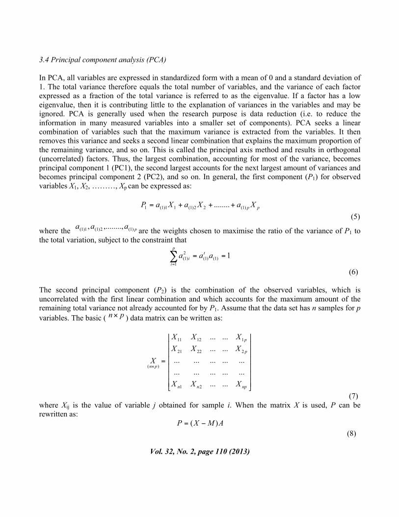
In this study, Varimax rotation was selected to maximize the sum of the variances of the squared loadings and thus enable us to seek the similarity of chemical components in sediment and soil samples. µ-SXRF spectra of the samples listed in Table 1 were analysed by PCA. The principal component patterns for Varimax rotated components of 30 samples composed of two PC, which account for 82.9 % and 17.0 % for the total of variances of PC1 and PC2 respectively. The contribution of PC1 and PC2 explains 99.9 % of total variance, and moreover PC1 is 4.87 times higher than PC2. Multi dimensional (MD) plots of PC1, PC2 and PC3 have been frequently employed as diagnostic tools of chemical sources in environmental samples (Marcosa et al., 2010; Pongpiachan, 2006; Pongpiachan et al., 2012; Pongpiachan et al., 2013; Tipmanee et al., 2012). MD distribution patterns of PCs can be used as a characteristic diagnostic parameter to identify their elemental distribution characteristics in soil and sediment samples. However, these MD plots, as well as HCA and PDF, should be used with great caution as physiochemical processes can alter elemental distribution pattern during their transport from the emission source to the receptor site. Apart from using only raw data of µ-SXRF spectra, a second approach was also pioneered by using the first-order derivative dataset for three-dimensional (3D) plots of PCs in order to minimize the above-mentioned uncertainties. In bi-polar plots of PC1 versus PC2 (see Figure 9), the vast majority of data points were clustered along the positive values of PC2 (y-axis) adjacent to 1.0 and subsequently decrease exponentially to positive side of PC1 (x-axis). The clearest features in MD plots (see Fig. 9-10) are: (i) 2D plots of samples No.23, No.31, No.39, No.72, No.78, No.5-21 and No.5-23, which were clustered close to

Vol. 32, No. 2, page 111 (2013)

each other. It seems rational to interpret this cluster as evidence of tsunami backwash deposit samples. (ii) 2D plots of CZS samples (i.e. No.Tub1, No.PK3, No.BN2, No.BP3) with the mixture of TMS samples (i.e. No.17, No.53, No.62) and OTD samples (i.e. No. BM1-Tsu, No.BM2-Tsu, No.BP3, No.BK5-Tsu, No.BM2-Post-Tsu). It appears reasonable to ascribe this cluster as a mixture of terrestrial components and marine deposits. This can be deduced as a consequence of inferior mixing process between tsunami backwash deposits and typical marine sediments after tsunami inundation; (iii) OTD samples are highly deviated from TMS and TBD samples but possess similar distribution pattern with those of CZS samples as noticeably illustrated in 3D plots of first-order derivative PCs (see Fig. 10). This can be explained by the high degree of similarity in elemental distribution between onshore tsunami deposits and coastal zone soils.

Fig. 9: Three-dimensional plots of principal components (PC) with raw data of typical marine

sediments (TMS), tsunami backwash deposits (TBD), on-shore tsunami deposits (OTD) and coastal zone soils (CZS).

4. SYNTHESIS AND CONCLUSIONS The above statistical analysis of collected data reveals that µ-SXRF spectra can yield authentic and valuable insight upon the terrestrial soils and/or marine sediments transportation processes affecting elemental distribution in the tsunami affected area. Subsequently, the authors support interpreting µ- SXRF spectra on the basis of various types of advanced statistical analyses rather than the simple use of raw spectra, which seems to be difficult for drawing any conclusions.

Vol. 32, No. 2, page 112 (2013)

Terrestrial)Soils)

Tsunami)Backwash)Deposits)

Tsunami)Backwash)Deposits)

The major conclusions that occur from this data interpretation are described as follows:

(a) The prominent µ-SXRF spectra features of Typical Marine Sediments (TMS), Tsunami Backwash Deposits (TBD), Onshore Tsunami Deposits (OTD) and Cluster Zone Soils (CZS) can be achieved only through the employment of first order derivative data.

(b) The analysis of Probability Distribution Function (PDF) for different sample categories shows

a clear influence of terrestrial soils and/or marine sediments transportation on elemental distribution.

(c) The Hierarchical Cluster Analysis (HCA) analysis of both raw and first order derivative data

successfully discriminate terrestrial components from typical marine sediments with the assistance of dendrographic classification.

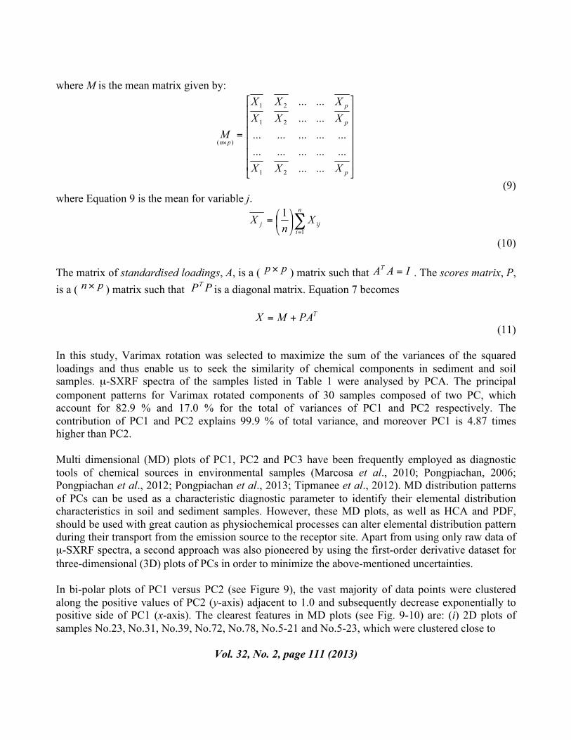
(d) The multi-dimensional plots of principal components (PCs) by using both raw and first order

derivative data highlights the characteristic features of onshore tsunami deposits and coastal zone soils as clearly demonstrated in Fig.9-10.

Fig. 10: Three-dimensional plots of principal components (PC) with the first-order derivative data of

typical marine sediments (TMS), tsunami backwash deposits (TBD), on-shore tsunami deposits (OTD) and coastal zone soils (CZS).

Vol. 32, No. 2, page 113 (2013)

5. ACKNOWLEDGEMENTS This work was performed with the approval of Deutsche Forschungsgemeinschaft (DFG, Grant SCHW/ 11-1) and National Research Council of Thailand (NRCT). The authors acknowledge Phuket Marine Biological Center (PMBC) for their support with ship time of RV Chakratong Tongyai and RV Boonlert Pasook, as well as other contributions and facilities during field measurements. We are greatful to Mrs. D. Sakuna for support during all cruises. The authors would also like to express special gratitude to Synchrotron Light Research Institute (Public Organization), Ministry of Science and Technology, Thailand for their contribution of µ-SXRF measurements. REFERENCES ABRANTES, F., ALT-EPPING, U., LEBREIRO, S., VOELKER, A. & SCHNEIDER, R. (2008). Mar. Geol. 249

(3–4), 283-293. BADIN, A. L., FAURE, P., BEDELL, J. P. & DELOLME, C. (2008). Sci. Total. Environ. 403, 178-187. BALSAM, W. L. & DEATON, B. C. (1991). Rev. Aquat. Sci. 4, 411-447. BALSAM, W. L. & BEESON, J. P. (2003). Deep. Sea. Res. Pat. I. 50, 1421-1444. BÖNING, P., BARD, E. & ROSE, J. (2007). Geochem. Geophy. Geosy. 8 (5),

DOI: 10.1029/2006GC001480. CHOOWONG, M., MURAKOSHI, N., HISADA, K., CHARUSIRI, P., DAORERK, V., CHAROENTITIRAT, T.,

CHUTAKOSITKANON, V., JANKAEW, K. & KANJANAPAYONT, P. (2007). J. Coastal. Res. 23(5), 1270–1276.

CHOOWONG, M., MURAKOSHI, N., HISADA, K., CHARUSIRI, P., CHAROENTITIRAT, T., CHUTAKOSITKANON, V., JANKAEW, K., KANJANAPAYONT, P. & PHANTUWONGRAJ, S. (2008a) Mar. Geol. 248 (3–4), 179–192.

CHOOWONG, M., MURAKOSHI, N., HISADA, K., CHAROENTITIRAT, T., CHARUSIRI, P., PHANTUWONGRAJ, S., WONGKOK, P., CHOOWONG, A., SUBSAYJUN,R., CHUTAKOSITKANON, V., JANKAEW, K. & KANJANAPAYONT, P. (2008b). Terra. Nova. 20, 141–149.

CHOOWONG, M., PHANTUWONGRAJ, S., CHAROENTITIRAT, T., CHUTAKOSITKANON, V., YUMUANG, S. & CHARUSIRI, P. (2009). Geomorphology. 104, 134–142.

FAGHERAZZI, S. & DU, X. (2007). Geomorphology. 99, 120-129. FELDENS, P., SCHWARZER, K., SZCZUCIŃSKI, W., STATTEGGER, K., SAKUNA, D. &

SOMGPONGCHAIYKUL, P. (2009). Polish. J. Enivron. 18, 63-68. FELDENS, P., SCHWARZER, K., SAKUNA, D., SZCZUCIŃSKI, W. & SOMPONGCHAIYAKUL, P. (2013).

Earth. Planets. Space. 64(10), 875-887. GOFF, C. C., ANDREW, A., SZCZUCIŃSKI, W., GOFF, J. & NISHIMURA, Y. (2012). Sediment. Geol. 282,

65-77. GRIFFIN, C., ELLIS, D., BEAVIS, S. & NANTES, Z.D. (2013). Ocean. Coast. Manage. 71, 176-186. JAGODZIŃSKI, R., STERNAL, B., SZCZUCIŃSKI, W., GOFF, C. C. & SUGAWARA, D. (2012). Sediment.

Geol. 282, 57-64. KANNGIEβER, B. & HASCHKE, M. (2006). Handbook of Practical X-ray Fluorescence Analysis, edited

by B. Beckhoff, B. Kanngieber, N. Langhoff, R. Wedell and H. Wolff, pp. 442-462. Berlin, Spinger-Verlag.

Vol. 32, No. 2, page 114 (2013)

MARCOSA, M. M., HARRISON, M. R., SCHUHMACHER, M., DOMINGO, L. J. & PONGPIACHAN, S. (2010). Sci. Total. Environ. 408, 2387-2393.

MATSUMARU, R., NAGAMI, K. & TAKEYA, K. (2012). IATSS. Res. 36 (1), 11-19. PONGPIAJUN, S. (2006). Atmospheric Chemistry of Semi-Volatile Organic Compounds in Urban and

Rural Air, University of Birmingham. PONGPIACHAN, S., THUMANU, K., KOSITANONT, C., SCHWARZER, K., PRIETZEL, J., HIRUNYATRAKUL, P.

& KITTIKOON, I. (2012). J. Anal. Methods. Chem. Article ID 659858, doi: 10.1155/2012/659858.

PONGPIACHAN, S., THUMANU, K., NA PHATTHALUNG, W., TIPMANEE, D., KANCHAI, P., FELDENS, P & SCHWARZER, K. (2013). Sci. Tsu. Haz. (ISSN 8775-6839), 32 (1), 39-57.

SAKUNA, D., SZCZUCIŃSKI, W., FELDENS, P., SCHWARZER, K. & KHOKIATTIWONG, S. (2012). Earth. Planets. Space. 64, 931-943.

SOLE, V. A., PAPILLON, E., COTTE, M., WALTER, PH., & SUSINI, J. (2007). Spectrochim. Acta B, 62, 63-68.

SOONTARANON, S. & RUGMAI, S. (2012). Small angle X-ray scattering at Siam photon laboratory, Chinese. J. Phys. 50 (2), 204–210, 2012.

SZCZUCIŃSKI, W., NIEDZIELSKI, P., RACHLEWICZ, G., SOBCZYŃSKI, T., ZIOŁA, A., KOWALSKI, A., LORENC, S. & SIEPAK, J. (2005). Environ. Geol. 49 (2), 321-331.

SZCZUCIŃSKI, W., CHAIMANEE, N., NIEDZIELSKI, P., RACHLEWICZ, G., SAISUTTICHAI, D., TEPSUWAN, T., LORENC, S. & SIEPAK, J. (2006). Pol. J. Environ. Stud. 15 (5), 793–810.

SZCZUCIŃSKI, W., NIEDZIELSKI, P., KOZAK, L., FRANKOWSKI, M., ZIOŁA, A. & LORENC, S. (2007). Environ. Geol. 53 (2), 253-264.

SZCZUCIŃSKI, W. (2012). Nat. Hazards Earth Syst. Sci. 60,115–133. TANCHARAKORN, S., TANTHANUCH, W., KAMONSUTTHIPAIJIT, N., WONGPRACHANUKUL, N., SOPHON,

M., CHAICHUAY, S., UTHAISAR, C. & YIMNIRUN, R. (2012). J. Synchrotron. Rad. 19, 536-540. TIPMANEE, D., DEELAMAN, W., PONGPIACHAN, S., SCHWARZER, K. & SOMPONGCHAIYAKUL, P. (2012).

Nat. Hazards Earth Syst. Sci. 12, 1441–1451. VÖTT, A., LANG, F., BRÜCKNER, H., PAPANASTASSIOU, G. K., MAROUKIAN, H., PAPANASTASSIOU, D.,

GIANNIKOS, A., HADLER, H., HANDL, M., NTAGERETZIS, K., WILLERSHÄUSER, T. & ZANDER, A. (2011). Quatern. Int. 242(1), 213-239.

Vol. 32, No. 2, page 115 (2013)