School bus crashworthiness - CORE

Graduate Theses, Dissertations, and Problem Reports

1998

School bus crashworthiness School bus crashworthiness

Ganesh R. Panneer West Virginia University

Follow this and additional works at: https://researchrepository.wvu.edu/etd

Recommended Citation Recommended Citation Panneer, Ganesh R., "School bus crashworthiness" (1998). Graduate Theses, Dissertations, and Problem Reports. 902. https://researchrepository.wvu.edu/etd/902

This Thesis is protected by copyright and/or related rights. It has been brought to you by the The Research Repository @ WVU with permission from the rights-holder(s). You are free to use this Thesis in any way that is permitted by the copyright and related rights legislation that applies to your use. For other uses you must obtain permission from the rights-holder(s) directly, unless additional rights are indicated by a Creative Commons license in the record and/ or on the work itself. This Thesis has been accepted for inclusion in WVU Graduate Theses, Dissertations, and Problem Reports collection by an authorized administrator of The Research Repository @ WVU. For more information, please contact [email protected].

https://researchrepository.wvu.edu/

https://researchrepository.wvu.edu/

https://researchrepository.wvu.edu/etd

https://researchrepository.wvu.edu/etd?utm_source=researchrepository.wvu.edu%2Fetd%2F902&utm_medium=PDF&utm_campaign=PDFCoverPages

https://researchrepository.wvu.edu/etd/902?utm_source=researchrepository.wvu.edu%2Fetd%2F902&utm_medium=PDF&utm_campaign=PDFCoverPages

mailto:[email protected]

School Bus Crashworthiness

Ganesh R. Panneer

Thesis submitted to the faculty of the College of Engineering and MineralResources at West Virginia University in partial fulfillment of the

requirements for the degree of

Master of Sciencein

Mechanical Engineering

Gregory Thompson, Ph.D., ChairJames Smith, Ph.D

Victor Mucino, Ph.D.

May 22, 1998Morgantown, West Virginia

Keywords: Crashworthiness, School Bus, Numerical Simulation

School Bus Crashworthiness

Ganesh R. Panneer

(ABSTRACT)

Numerical simulation of automotive crashes play an important role in reducing thecost and time taken for predicting the results of a collision. Computer simulation of avehicle requires that the vehicle structure be modeled in a finite element package bydiscretizing the geometry into a number of elements.

Every day thousands of children travel to school and school related events by bus.Not necessarily all the journeys are short and safely driven. The potential for seriousinjuries is possible in the event of a crash. The severity of injury in an offset frontalimpact is higher than the full frontal impact, because of the offset in the principaldirection of the impact force.

A finite element model of a school bus was created in I-DEAS Master Series. Thebody structure was modeled with the rib structure and the body skin. The chassis wasmodeled with engine, gearbox, drive train, and axles. The body structure was attached tothe chassis to create a complete finite element model of the bus. IDEADYN was used asa translator to write a LS-DYNA3D input file. Full frontal and offset frontal impacts weresimulated in LS-DYNA3D with an initial velocity of 56 km/hr against a rigid wall. Sincehourglassing energy was high in the previous results, a higher order integration was donefor all the thin shell elements with Hughes-Liu SR thin shell elements. LS-TAURUS wasused to post process the results obtained from the simulation. The results from theanalysis included nodal displacement, velocity and accelerations, energy absorption, rigidwall forces, and occupant intrusion. The results from the two cases, with and withouthourglassing energy, were compared.

ii

‘

Acknowledgements

I would like to take this opportunity to express my deepest gratitude to my research

advisor, Dr. Gregory J. Thompson, for his constant support, enthusiasm and motivation.

His encouragement and guidance have helped me achieve my academic goals and at the

same time made me a more complete person.

This gives me a platform to thank Dr. James E. Smith who by his timely support

provided me with one of the best environments to carry out research in the area of

crashworthiness. His guidance helped me overcome many of the problems I faced during

the course of my thesis work.

I would also like to thank my committee member Dr. Victor H. Mucino for his

guidance and support during my research work.

Thanks are also due to Joanna Davis-Swing and Jack Connolly for all the help

extended.

iii

Table of Contents

Acknowledgements................................................................................................................................. ii

Table of Contents .................................................................................................................................. iii

List of Figures .........................................................................................................................................v

List of Tables..........................................................................................................................................ix

Nomenclature ..........................................................................................................................................x

CHAPTER 1 – INTRODUCTION ..........................................................................................................1

CHAPTER 2 – LITERATURE REVIEW ..............................................................................................7

2.1 HIGHWAY SCHOOL BUS ACCIDENT REPORTS...........................................................................72.1.1 VAN BASED TEST .........................................................................................................82.1.2 TYPE A PILLAR CRASH .................................................................................................92.1.3 CRASHWORTHINESS STUDY OF TYPE A BUSES ...............................................................92.1.4 TYPE A SIDE IMPACT ..................................................................................................102.1.5 TYPE A CRASH WITH A LOCOMOTIVE...........................................................................10

2.2 PRIOR BUS/TRUCK NUMERICAL MODELS ..............................................................................112.3 MODELING APPROACHES TO VEHICLE CRASHWORTHINESS SIMULATION ................................132.4 SOFTWARE PACKAGES FOR VEHICLE CRASHWORTHINESS SIMULATION ..................................35

CHAPTER 3 – THEORY OF LS-DYNA3D.........................................................................................37

3.1 FEM PRELIMINARIES .............................................................................................................373.2 SOLID ELEMENTS .................................................................................................................403.3 HOUR GLASS CONTROL ........................................................................................................423.4 TIME INTEGRATION ..............................................................................................................423.5 CENTRAL DIFFERENCE METHOD ...........................................................................................443.6 NUMERICAL ANALYSIS .........................................................................................................45

3.6.1 LINEAR AND NON-LINEAR ANALYSIS ..........................................................................463.7 CONTACT IMPACT ALGORITHM IN LS-DYNA3D ...................................................................47

CHAPTER 4 – FINITE ELEMENT MODEL OF THE BUS ..............................................................50

4.1 INTRODUCTION TO FEM PROCEDURE .....................................................................................504.2 PRE-PROCESSING..................................................................................................................51

4.2.1 DATA COLLECTION.....................................................................................................524.2.2 PRE-PROCESSING IN I-DEAS.......................................................................................524.2.3 BOUNDARY CONDITIONS.............................................................................................62

4.3 ANALYSIS ............................................................................................................................654.3.1 MATERIAL MODELS IN LS-DYNA3D .........................................................................664.3.1.1 MATERIAL 1 ............................................................................................................66

4.4 POST-PROCESSING................................................................................................................674.4.1 LS-TAURUS .............................................................................................................67

CHAPTER 5 - RESULTS AND DISCUSSION....................................................................................69

5.1 INTRODUCTION.....................................................................................................................695.2 FULL FRONTAL IMPACT WITH BELYTSCHKO -TSAY THIN SHELL ELEMENTS ............................72

iv

5.3 OFFSET FRONTAL IMPACT WITH BELYTSCHKO -TSAY THIN SHELL ELEMENTS.........................955.4 HIGHER ORDER INTEGRATION FOR THIN SHELL ELEMENTS..................................................1165.5 FULL FRONTAL IMPACT WITH HUGHES-LIU SR THIN SHELL ELEMENTS...............................1175.6 OFFSET FRONTAL IMPACT WITH HUGHES-LIU SR THIN SHELL ELEMENTS ...........................142

CHAPTER 6 –CONCLUSIONS AND RECOMMENDATIONS ......................................................165

6.1 CONCLUSIONS ....................................................................................................................165

CHAPTER – 8 REFERENCES ..........................................................................................................171

APPENDIX A – FMVSS FOR SCHOOL BUS...................................................................................176

APPENDIX B – CONDENSED LS-DYNA3D INPUT FILE .............................................................177

APPENDIX C - YIELD STRESS OF MATERIALS .........................................................................188

VITA....................................................................................................................................................189

APPROVAL OF EXAMINING COMMITTEE .................................................................................190

v

List of Figures

Fig 2.1 Influence of mesh density on displacement..................................................................................16Fig 2.2 Graph showing the deceleration force varying linearly with time. ................................................18Fig 2.3 Deformation of the Suzuki Sidekick finite element model. ..........................................................21Fig 2.4 New emergency exit. ..................................................................................................................30Fig 3.1 Displacement of a body from position B at time t=0 to position b at time t=T. .............................37Fig 3.2 Eight noded solid element...........................................................................................................41Fig 3.3 Simple spring mass system with a damper...................................................................................44Fig 3.4 Free body diagram of the spring mass system...............................................................................44Fig 4.1 Flow chart of the finite element method. .....................................................................................50Fig 4.2 Frame structure of the bus with springs and fuel tank. .................................................................53Fig 4.3 Front axle with tires....................................................................................................................54Fig 4.4 Radiator, engine and gearbox with propeller shaft. ......................................................................55Fig 4.5 Rear axle with tires. ....................................................................................................................56Fig 4.6 Bumper finite element model. .....................................................................................................57Fig 4.7 Fire wall finite element model.....................................................................................................58Fig 4.8 Bus body structure......................................................................................................................59Fig 4.9 Bus body with sheet metal over the ribs. .....................................................................................60Fig 4.10 Complete finite element model of the bus with different parts assembled. ..................................61Fig 4.11 Flow chart for file translation from I-DEAS to LS-DYNA3D. ...................................................64Fig 4.12 File Organization for LS-TAURUS. ..........................................................................................68Fig 5.1 Full finite element model of the school bus with coordinate system. ............................................71Fig 5.2 Front view at time = 0 msec of the bus subjected to a full frontal impact at a velocity of 56

km/hr. .......................................................................................................................................72Fig 5.3 Front view at time = 9 msec of the bus subjected to a full frontal impact at a velocity of 56

km/hr. .......................................................................................................................................73Fig 5.4 Front view at time = 18 msec of the bus subjected to a full frontal impact at a velocity of

56 km/hr....................................................................................................................................74Fig 5.5 Front view at time = 27 msec of the bus subjected to a full frontal impact at a velocity of



56 km/hr....................................................................................................................................77Fig 5.8 Front view at time = 54 msec of the bus chassis subjected to a full frontal impact at a

velocity of 56 km/hr. .................................................................................................................78Fig 5.9 Front view at time = 72 msec of the bus chassis subjected to a full frontal impact at a

velocity of 56 km/hr. ................................................................................................................79Fig 5.10 Front view at time = 90 msec of the bus subjected to a full frontal impact at a velocity of

56 km/hr....................................................................................................................................80Fig 5.11 Figure showing the side view of the bus at time = 45 msec for full frontal impa7ct. ....................81Fig 5.12 Figure showing the top view of the bus at time = 45 msec for full frontal impact........................82Fig 5.13 Figure showing the deformation of the frame at time =90 msec for a full frontal impact. ............82Fig 5.14 Figure showing the VonMises stress plot in the front end of the frame at time = 45 msec. ..........83Fig 5.15 Relative displacement between the frame and the front tire........................................................84Fig 5.16 Relative displacement between the front tire and the rear tire (pitching).....................................85Fig 5.17 Z displacement for nodes in the front of vehicle. .......................................................................86Fig 5.18 Z displacement for nodes in the middle of vehicle. ....................................................................86Fig 5.19 Z displacement for nodes in the rear of vehicle. .........................................................................87Fig 5.20 Z velocity for nodes in the front of vehicle. ...............................................................................88Fig 5.21 Z velocity for nodes in the middle of vehicle. ............................................................................88

vi

Fig 5.22 Z velocity for nodes in the rear of vehicle..................................................................................89Fig 5.23 Z acceleration for nodes in the front of vehicle. .........................................................................90Fig 5.24 Z acceleration for nodes in the middle of vehicle. ......................................................................90Fig 5.25 Z acceleration for nodes in the rear of vehicle............................................................................91Fig 5.26 Z rigid body velocity for materials(Refer to Table 5.1 for table of materials)..............................92Fig 5.27 Z rigid body velocity for a bus subjected to a full frontal impact at 56 km/hr..............................92Fig 5.28 Internal energy for materials (refer to Table 5.1 for table of materials). ......................................93Fig 5.29 Internal, kinetic, and the total energies for a full frontal impact. .................................................94Fig 5.30 Total internal energy distribution at time = 90 msec of the bus subjected to a full frontal

impact. ......................................................................................................................................95Fig 5.31 Front view at time = 9 msec of the bus subjected to an offset frontal impact at a velocity

of 56 km/hr................................................................................................................................96Fig 5.32 Front view at time = 18 msec of the bus subjected to an offset frontal impact at a velocity




of 56 km/hr..............................................................................................................................100Fig 5.36 Front view at time = 54 msec of the bus subjected to an offset frontal impact at a velocity



of 56 km/hr..............................................................................................................................103Fig 5.39 Side view at time=45 msec of the bus subjected to an offset frontal impact. .............................104Fig 5.40 Top view at time=45 msec of the bus subjected to an offset frontal impact...............................104Fig 5.41 Relative displacement between the nodes in the right and the left tires in front axle..................105Fig 5.42 Relative displacement between the front tire and the rear tire..................................................106Fig 5.43 Relative displacement between the nodes in the fire wall and the right tire...............................106Fig 5.44 Z displacement for the nodes in the front of the vehicle. ..........................................................107Fig 5.45 Z displacement for the nodes in the middle of the vehicle. .......................................................108Fig 5.46 Z displacement for the nodes in the rear of the vehicle.............................................................108Fig 5.47 Z velocity for the nodes in the front of the vehicle. ..................................................................109Fig 5.48 Z velocity for the nodes in the middle of the vehicle. ...............................................................110Fig 5.49 Z velocity for the nodes in the rear of the vehicle. ...................................................................110Fig 5.50 Z acceleration for nodes in the front of the vehicle...................................................................112Fig 5.51 Z acceleration for the nodes in the middle of the vehicle..........................................................112Fig 5.52 Z acceleration of the nodes in the rear of the vehicle................................................................113Fig 5.53 Z rigid body velocity for materials (Refer to Table 5.1 for table of materials)...........................114Fig 5.54 Internal energy absorbed by materials (Refer to Table 5.1 for table of materials)......................115Fig 5.55 Kinetic, internal and the total energies for an offset frontal impact. ..........................................116Fig 5.56 Total internal energy distribution at time = 90 msec of the bus subjected to an offset

frontal impact. .........................................................................................................................116Fig 5.57 Front view at time = 0 msec of the bus subjected to a full frontal impact with Hughes-Liu

SR thin shells. .........................................................................................................................118Fig 5.58 Front view at time = 9 msec of the bus subjected to a full frontal impact with Hughes-Liu

SR thin shells. .........................................................................................................................119Fig 5.59 Front view at time = 18 msec of the bus subjected to a full frontal impact with Hughes-

Liu SR thin shells. ...................................................................................................................120Fig 5.60 Front view at time = 27 msec of the bus subjected to a full frontal impact with Hughes-

Liu SR thin shells. ...................................................................................................................121Fig 5.61 Front view at time = 36 msec of the bus subjected to a full frontal impact with Hughes-

Liu SR thin shells. ...................................................................................................................122

vii

Fig 5.62 Front view at time = 45 msec of the chassis of the bus subjected to a full frontal impactwith Hughes-Liu SR thin shells................................................................................................123

Fig 5.63 VonMises stress plot in the front end of the frame at time = 45 msec for a full frontalimpact with Hughes-Liu SR thin shells. ...................................................................................125

Fig 5.64 Side view at time = 45 msec of the bus subjected to a full frontal impact with Hughes-Liu SR thin shells. ...................................................................................................................126

Fig 5.65 Top view at time = 45 msec of the bus subjected to a full frontal impact with Hughes-LiuSR thin shells. .........................................................................................................................126

Fig 5.66 Relative displacement between the hood and the frame for a full frontal impact withHughes-Liu SR thin shells. ......................................................................................................127

Fig 5.67 Z relative displacement between the frame and the front tire for a full frontal impact withHughes-Liu SR thin shells. ......................................................................................................128

Fig 5.68 Z displacement for the nodes in the front of the vehicle for full frontal impact withHughes-Liu SR thin shells. ......................................................................................................129

Fig 5.69 Z displacement for the nodes in the middle of the vehicle for full frontal impact withHughes-Liu SR thin shells. ......................................................................................................129

Fig 5.70 Z displacement for the nodes in the rear of the vehicle for full frontal impact withHughes-Liu SR thin shells. ......................................................................................................130

Fig 5.71 Z velocity for the nodes in the front of the vehicle for full frontal impact with Hughes-Liu SR thin shells. ...................................................................................................................131

Fig 5.72 Z velocity for the nodes in the middle of the vehicle for full frontal impact with Hughes-Liu SR thin shells. ...................................................................................................................131

Fig 5.73 Z velocity for the nodes in the rear of the vehicle for full frontal impact with Hughes-LiuSR thin shells. .........................................................................................................................132

Fig 5.74 Z acceleration for the nodes in the front of the vehicle for full frontal impact withHughes-Liu SR thin shells. ......................................................................................................133

Fig 5.75 Z acceleration for the nodes in the middle of the vehicle for full frontal impact withHughes-Liu SR thin shells. ......................................................................................................133

Fig 5.76 Z acceleration for the nodes in the rear of the vehicle for full frontal impact with Hughes-Liu SR thin shells. ...................................................................................................................134

Fig 5.77 X rigid body velocities of materials for a full frontal impact with Hughes-Liu SR thinshells. ......................................................................................................................................135

Fig 5.78 Y rigid body velocities of materials for a full frontal impact with Hughes-Liu SR thinshells. ......................................................................................................................................135

Fig 5.79 Z rigid body velocities of materials for a full frontal impact with Hughes-Liu SR thinshells. ......................................................................................................................................136

Fig 5.80 Total rigid body velocity for materials for a full frontal impact with Hughes-Liu SR thinshells. ......................................................................................................................................136

Fig 5.81 Global X rigid body velocity for a full frontal impact with Hughes-Liu SR thin shell. ..............137Fig 5.82 Global Y rigid body velocity for a full frontal impact with Hughes-Liu SR thin shell. ..............138Fig 5.83 Global Z rigid body velocity for a full frontal impact with Hughes-Liu SR thin shell. ..............138Fig 5.84 Global total rigid body velocity for a full frontal impact with Hughes-Liu SR thin shells..........139Fig 5.85 Material internal energy absorption for a full frontal impact with Hughes-Liu SR thin

shells. ......................................................................................................................................140Fig 5.86 Global energies for a full frontal impact with Hughes-Liu SR thin shells. ................................141Fig 5.87 Total internal energy distribution at time = 45 msec of the bus subjected to a full frontal

impact with Hughes-Liu SR thin shells. ...................................................................................141Fig 5.88 Front view at time = 0 msec of the bus subjected to an offset frontal impact with Hughes-

Liu SR thin shells. ...................................................................................................................142Fig 5.89 Front view at time = 9 msec of the bus subjected to an offset frontal impact with Hughes-

Liu SR thin shells. ...................................................................................................................143Fig 5.90 Front view at time = 18 msec of the bus subjected to an offset frontal impact with

Hughes-Liu SR thin shells. ......................................................................................................144Fig 5.91 Front view at time = 27 msec of the bus subjected to an offset frontal impact with

Hughes-Liu SR thin shells. ......................................................................................................145

viii

Fig 5.92 Front view at time = 36 msec of the bus subjected to an offset frontal impact withHughes-Liu SR thin shells. ......................................................................................................147



Fig 5.95 Side view at time = 54 msec of the bus subjected to an offset frontal impact with Hughes-Liu SR thin shells. ...................................................................................................................150

Fig 5.96 Top view at time = 54 msec of the bus subjected to an offset frontal impact with Hughes-Liu SR thin shells. ...................................................................................................................150

Fig 5.97 Relative displacement between the right wheel and the left wheel (axle rotation) for anoffset frontal impact with Hughes-Liu SR thin shell elements...................................................151

Fig 5.98 Relative displacement between the front tires and the rear tires (pitching) for an offsetfrontal impact with Hughes-Liu SR thin shell elements. ...........................................................152

Fig 5.99 Z displacement for the nodes in the front of the vehicle for an offset frontal impact withHughes-Liu SR thin shells. ......................................................................................................153

Fig 5.100 Z displacement for the nodes in the middle of the vehicle for an offset frontal impactwith Hughes-Liu SR thin shells................................................................................................153

Fig 5.101 Z displacement for the nodes in the rear of the vehicle for an offset frontal impact withHughes-Liu SR thin shells. ......................................................................................................154

Fig 5.102 Z velocity for the nodes in the front of the vehicle for an offset frontal impact withHughes-Liu SR thin shells. ......................................................................................................155

Fig 5.103 Z velocity for the nodes in the middle of the vehicle for an offset frontal impact withHughes-Liu SR thin shells. ......................................................................................................155

Fig 5.104 Z velocity for the nodes in the rear of the vehicle for an offset frontal impact withHughes-Liu SR thin shells. ......................................................................................................156

Fig 5.105 Z acceleration for the nodes in the front of the vehicle for an offset frontal impact withHughes-Liu SR thin shells. ......................................................................................................157

Fig 5.106 Z acceleration for the nodes in the middle of the vehicle for an offset frontal impactwith Hughes-Liu SR thin shells................................................................................................157

Fig 5.107 Z acceleration for the nodes in the rear of the vehicle for an offset frontal impact withHughes-Liu SR thin shells. ......................................................................................................158

Fig 5.108 Material rigid body velocity of parts for an offset frontal impact with Hughes-Liu SRthin shells. ...............................................................................................................................159

Fig 5.109 Global X rigid body velocity of the bus for an offset frontal impact with Hughes-LiuSR thin shells. .........................................................................................................................160

Fig 5.110 Global Y rigid body velocity of the bus for an offset frontal impact with Hughes-LiuSR thin shells. .........................................................................................................................160

Fig 5.111 Global Z rigid body velocity of the bus for an offset frontal impact with Hughes-Liu SRthin shells. ...............................................................................................................................161

Fig 5.112 Global total rigid body velocity of the bus for an offset frontal impact with Hughes-LiuSR thin shells. .........................................................................................................................161

Fig 5.113 Material internal energy of parts for an offset frontal impact with Hughes-Liu SR thinshells. ......................................................................................................................................163

Fig 5.114 Internal , kinetic and total energies for an offset frontal impact with Hughes-Liu SR thinshells. ......................................................................................................................................163

Fig 5.115 Total internal energy distribution at time = 45 msec of the bus subjected to an offsetfrontal impact with Hughes-Liu SR thin shells. ........................................................................164

Fig 6.1 Instability in the total energy of the system with high hour glassing. ..........................................166

ix

List of Tables

Table 3.1 Operation count for hourglassing types. ...................................................................................42Table 4.1 Prioritization of the components for modeling. ........................................................................53Table 4.2 Component wise mesh density.................................................................................................62Table 4.3 Control switches for LS-DYNA3D..........................................................................................66Table 5.1 Parts and part numbers. ...........................................................................................................70

x

Nomenclature

jn - Normal outward unit vector of boundary element

ix&& - Acceleration [m/s2]

if - Body force [N]

iv - Initial velocity [m/s]

ix - Current velocity [m/s]

ik - Number of Nodesc - Damping coefficient [N.s/m]k - Linear stiffness [N/m]M - Diagonal mass matrix [Kg]

nP - External body and force loads [N]nF - Stress divergence vector [N]nH - Hour glass resistance [N]

u - Displacement [m]u& - Velocity [m/s]u&& - Acceleration [m/sec2]

Greekj,ijσ - Cauchy Stress [N/m2]

ρ - Density [Kg/m3]

jφ - Shape function

β - Parametric coordinatesη - Parametric coordinatesΓ - Parametric coordinates

1

CHAPTER 1 – INTRODUCTION

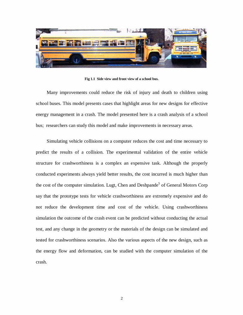
Every day thousands of children travel to school and school related events by bus.

An example of a typical school bus is shown in Figure 1.1. Since 1985, 1478 people have

died in school bus related crashes, an average of 134 fatalities per year26. Eleven percent

of these fatalities were the occupants of the school bus, an average of 14 deaths per year.

Impacts to the front of the vehicle occur in 47 percent of fatal school bus related crashes,

impacts to the rear of the vehicle occur in 7 percent of the crashes, and impact to the side

of the school bus occur in 15 percent of the crashes. Extensive research in passenger car

crashworthiness has improved automobile safety to the point where occupants in a family

sedan involved in an accident at relatively low speed will almost likely survive with only

minor injuries. However, school bus crashworthiness has received much less attention,

resulting in fewer improvements in the design and analysis of school buses.

The model presented here is the finite element model of a school bus, which was

studied for different crash scenarios and the numerical requirements. This model shows

the deformation and energy flow on the school bus in the event of a crash. The different

crash scenarios that were studied are the full frontal collision against a rigid wall and the

offset frontal collision against a rigid wall. In the full frontal rigid wall collision, the rigid

wall modeled is infinitely rigid and the wall extends from positive infinity to negative

infinity in the directions perpendicular to the rigid wall normal. The rigid wall normal is

parallel but in opposite direction to the velocity vector of the vehicle. In the offset frontal

collision, the rigid wall extends from the bus front centerline past the right side.

2

Fig 1.1 Side view and front view of a school bus.

Many improvements could reduce the risk of injury and death to children using

school buses. This model presents cases that highlight areas for new designs for effective

energy management in a crash. The model presented here is a crash analysis of a school

bus; researchers can study this model and make improvements in necessary areas.

Simulating vehicle collisions on a computer reduces the cost and time necessary to

predict the results of a collision. The experimental validation of the entire vehicle

structure for crashworthiness is a complex an expensive task. Although the properly

conducted experiments always yield better results, the cost incurred is much higher than

the cost of the computer simulation. Lugt, Chen and Deshpande5 of General Motors Corp

say that the prototype tests for vehicle crashworthiness are extremely expensive and do

not reduce the development time and cost of the vehicle. Using crashworthiness

simulation the outcome of the crash event can be predicted without conducting the actual

test, and any change in the geometry or the materials of the design can be simulated and

tested for crashworthiness scenarios. Also the various aspects of the new design, such as

the energy flow and deformation, can be studied with the computer simulation of the

crash.

3

During the design stage of a vehicle, a numerical simulation and / or an experiment

on a prototype can be done. Numerical modeling of the vehicle allows changes in the

design to be incorporated at the cost of the CPU run, whereas the experimental

crashworthiness test requires that each new prototype be manufactured and crashed. On

the other hand, the final stage of design validation requires an experimental

crashworthiness test, and the computer simulation is not an equivalent for this test.

During the design stage of a vehicle, the structural configuration may change, and if an

experimental prototype were to be built for each stage, it would be exorbitantly

expensive. Igarashi4 of Suzuki Motor Co worked on the structural analysis of the Suzuki

Sidekick at various stages of development and design where the numerical simulations

were used at the earlier stages of design and testing and evaluation at the last stage of the

development.

Each vehicle behaves differently under different collision events. Some of the

vehicles may prove to be good against frontal impact but not against side impact and vice

versa. The deformation and damage also differ from vehicle to vehicle. An accident

reconstruction is possible by visiting the scene of an accident and hence deducing the

events before the accident from the resulting wreck. Computer simulation allows not only

visualization of the damage during the event, but also analysis of other factors like

damage to the occupant and energy absorbed by different components of the vehicle.

The finite element method has been successfully used since the 1960’s to predict

the structural and dynamic behavior of beams and other members. This method of

computer simulation reduced the time and the cost of experiments that would be

conducted on these members to test their strength and other mechanical properties.

4

Computer programs for crashworthiness were first developed around 1970. The finite

element codes were written using a programming language and they were altered to the

needs of the developer. They were run in main frame computers in those days, which

took several hours to finish the computation. With the advent of supercomputers, even

though the models are more complex, the computation has become easier and less

expensive than it was previously.

The term crashworthiness by itself means the structural integrity of the member

against crash and impact forces. Related to a vehicle, crashworthiness means the behavior

of the vehicle in a collision with another vehicle or other object. The crashworthiness of

a vehicle is measured by its ability to absorb energy and prevent any possible object

intrusion causing an injury to the occupant. Crashworthiness studies currently use high-

speed digital cameras to capture pictures since a high speed collision at a velocity of

about 35 mph takes place only for about 60 to 80 milliseconds. Also, using of dummy

models of different sizes has been extremely useful because researchers can study the

impact on the human body and the possible injuries to them. Tests have been conducted

with various automobile models for different kinds of collisions, and a large database had

been developed by various research institutions which could be used for the study of

collision in the happening of the same event elsewhere.

Computer simulation of a vehicle requires that the vehicle structure be modeled in a

finite element package by discretizing the geometry into a number of elements. To save

the time and cost of computing, it is absolutely necessary to model only the components

that play a vital role in the crash scenario. Components that come into direct contact with

the impacting structure play an important role in energy absorption; other components

5

that have a substantially smaller mass compared to the mass of the vehicle can be

neglected. Due to high deformation rates, the time step required for analyzing the event

should be small which is computationally expensive.

RESEARCH OBJECTIVES

The research objectives of the following thesis are as follows.

1. Create a finite element model of the school bus in I-DEAS Master Series

and use LS-DYNA3D to study the crashworthiness of the model in various

collision events.

2. Run the analysis in the software for various crash scenarios.

3. Determine the numerical requirements.

4. Study the predicted behavior of the vehicle for deformation, energy

distribution, energy flow, rigid wall energy absorption, and acceleration

plots of various components.

5. Compare the results with the available data and standard crashworthiness

analysis output.

Preprocessing of the model was created in I-DEAS Master Series15. Drawings were

obtained from a manufacturer of a common 60-seat school bus, which is used for student

transportation at West Virginia University and thousands of school districts throughout

the United States. Along with the drawings, the dimensions of the components were

6

measured by hand. The I-DEAS model information was translated into a LS-DYNA3D

model with the translator IDEADYN12. After the solution phase, the preprocessing was

performed in LS-TAURUS16 and the results were presented.

7

CHAPTER 2 – LITERATURE REVIEW

Automobile manufacturers have used the finite element method in recent years to

study crash characteristics of automobiles. This technique has helped them reduce the

cost for testing each prototype that has to be manufactured during different stages of

design. Possible occupant injuries can be determined by studying the deformation

characteristics of the vehicle and the intrusion of parts into the occupant area after the

crash. If there is a possibility of serious injury to the occupant, redesign can be carried out

by simulation and also by testing the vehicle and comparing the results.

2.1 HIGHWAY SCHOOL BUS ACCIDENT REPORTS

Highway accident reports were obtained from National Technical Information

Service18 (NTIS) for accidents that involved school buses. These accident reports from

NTIS give a detailed investigation of the accident scenario, the analysis of the accident

and various factors that influenced the accident, findings, probable causes and

recommendations to avoid similar events in the future. Some of these reports give a

picture of the deformed school bus after the accident. They also provide an explanation of

the accident scene to aid visualization of the event. The investigation of the accident is

conducted by tracking the driving records and other information about the school bus

driver and the driver of the vehicle that was involved in the accident. The velocities of the

vehicles before the accident are deduced from the tire patch and deformation of the

vehicles after the accident. Reports are checked for the year in which these accidents

occurred, to make sure that the contents and the model of the bus involved in the accident

were not very old to make a comparison with the results obtained from these simulations.

8

These reports are the only data found for the comparison of the crashworthiness

simulation results for this project. Though the National Highway Traffic Safety

Administration (NHTSA) conducts several tests on school buses by crashing them, none

of them were looked in the perspective of the crashworthiness of the whole bus in

entirety.

2.1.1 VAN BASED TEST

Van based school buses are classified as Type A school buses where the gross

vehicle weight is less than 4545 kg (10,000 lbs) and designed for carrying ten or more

passengers. The school bus simulated in this project is called the Type C school bus or

the conventional school bus whose gross vehicle weight is more than 4545 kg (10,000

lbs) and designed for carrying more than ten passengers. All of the engine and engine

components are in front of the windshield, and the entrance door is behind the front

wheels. A crashworthiness test was conducted on a van based school bus (Type A) by the

National Transportation Safety Board (NTSB); however the bus model was not the same

as the one simulated in this project (Type C). Tests are often conducted to check the

brakes in the vehicle, damage to the fuel tank in the vehicle, hand rail designs, safety belt

use and joint strength. The Federal Motor Vehicle Safety Standards11 (FMVSS) are

defined for the performance of various systems of the bus like the hydraulic brake

system, air brake system, safety belt assemblies, window retention and release, bus body

joint strength, fuel system integrity, etc. A list of Federal Motor Vehicle Safety Standards

is listed in Appendix A.

9

2.1.2 TYPE A PILLAR CRASH

A highway accident investigation reports the loss of control and collision of a small

school bus (Type A) with a guard rail and sign pillar on November 11, 198527. The

activities of the school bus driver were investigated first with a detailed investigation on

the background of the driver. The vehicle was investigated for any damage, and the

highway weather and road conditions are also take into account. The pitman arm that

controls the vehicle steering was subjected to a metallurgical tests, which did not show

any preexistent failure of the component. The bus body was forced off of the chassis of

the bus, which had positive safety results since crash forces transmitted to the school bus

body were reduced. It was concluded that the school bus driver was driving the bus under

the influence of alcohol, which was the cause for the accident. This report does not look

in to the crashworthiness perspective of the accident and it does not give any picture of

the final deformed shape of the bus.

2.1.3 CRASHWORTHINESS STUDY OF TYPE A BUSES

The National Transportation Safety Board (NTSB) performed a safety study on the

crashworthiness of small post standard school buses28. The crashworthiness study was

conducted on a Type A school bus that weighed less than 4545 kg (10,000 lbs) and

designed to carry more than ten passengers. A small post standard school bus was

crashed and the damage to the exterior and the interior of the bus was documented and

analyzed, in relationship to each passenger’s seating position. For each occupant, the

investigators attempted to determine whether a restraint system was used, whether it was

used correctly, the probable cause of injury, and the nature and severity of the injury

sustained. Because of the differences in the size, mass and exterior features, the findings

10

from a small school bus cannot be extrapolated to a large school bus. It was concluded

that the small school buses involved in the accidents investigated provided good crash

protection.

2.1.4 TYPE A SIDE IMPACT

A highway accident investigation reports the collision of a small school bus (Type

A) with a tractor-semi trailer on November 10, 199329. The investigation reported the

activities of the school bus driver before the accident and the condition of the bus; before

the event a 72 hour history of both the drivers was investigated along with the work

experience and the driving record of the drivers. The school bus was damaged along the

doorway side of the body from a side impact. The contact deformation began at 22 inches

from the rear corner of the doorway and extended up to 96 inches, approximately equal to

the width of the tractor trailer. The maximum intrusion into the impact side of the bus

was 29 inches. An analysis of the sequence of events was made, and it was concluded

that the right front vertical support structure obscured the bus driver’s view for 5 to 7

seconds before the collision and this was the cause of the accident.

2.1.5 TYPE A CRASH WITH A LOCOMOTIVE

A highway accident investigation reports the collision of a locomotive with a school

bus (Type A) at a railroad grade crossing on October 25, 199530. The investigation

reported the activities of the school bus driver before the accident and the condition of the

school bus before the accident. An investigation was also made of the train crew and the

mechanical conditions of the train. Analysis was made of the school bus driver’s

performance, road design, rail road-highway sign interaction, and other factors that might

have caused the accident. It was concluded that the bus driver did not heed to the

11

warnings that a train was approaching the crossing and hence caused the accident. Also

the training provided by the school district to the bus driver during the emergency was

ineffective.

2.2 PRIOR BUS/TRUCK NUMERICAL MODELS

Trucks and buses were not modeled completely to study the crashworthiness of the

vehicle structure. In some cases, only the occupant area was modeled with simple beam

elements that could help to study the structural integrity of the bus. The National

Highway Traffic Safety Administration (NHTSA) reports that 1,478 people have died in

school bus related crashes since 1985, out of which 11 percent were occupants of school

buses11. However NHTSA, has conducted tests and setup standards for the various

components of the bus like the fuel tank, brake system, safety belt assemblies, and bus

body joint strength.

Monasa1 of the Civil Engineering department of Michigan Technological

University and McGuire of the Structural Engineering department of the Cornell

University in 1986 modeled the passenger compartment of a small bus. This model was

created to study the collapse performance and the structural integrity of the model, which

could determine the ultimate failure load and the deflection characteristics under

specified loading conditions. The passenger compartment of the bus was mounted on and

supported by a separate chassis. Interactive computer graphics were used to preprocess

and post process the model. The data was input through a graphic user interface and not

through digital means. A preprocessor called FRAME3D was used and solved in a

software called ANALYSE. A roll over load was applied at a node and the deformed

12

shape was determined. A program called SLD3D, which could perform a full range of

analysis from linear elastic to non-linear analysis, was used to solve the model. The

program was able to account for both types of non-linearity (i.e) geometric non-linearity

and material non-linearity. The program incorporates the material non-linearity by

attaching plastic hinges at the ends of the elements. Including a flexural member

geometrical stiffness matrix into the direct stiffness method incorporates geometric non-

linearity. The results showed a parellelogramming mode of deformation under the roll

over load and a passenger safety compartment in the structure was determined.

Mahesh7, Subash and Yan of Concordia University worked on the crashworthiness

enhancement in a car-truck collision by providing an energy dissipative under-ride guard.

The energy dissipative under-ride guard helps to absorb energy when a lightweight

vehicle such as a car is involved in a collision with a heavy truck. Since the kinetic

energy of the heavy vehicle is very high compared to that of the car, the possibility of

heavy damage to the occupants in the smaller vehicle is high. So, energy dissipative

under-ride guards with hydraulic dampers attached to the rear side of the under-ride

guards provide excellent energy absorbing capabilities. By using the basic equations of

motion, and equating the moment of the momentum after the impact in the under-ride

guard, the velocity of the car at the point of impact was determined. Also the magnitude

of the acceleration of the car mass and the dissipated energy under direct impact is

determined. Also two different kinds of conventional under-ride guards were modeled in

LS-DYNA3D and the results of the conventional guard were compared to those of the

proposed under-ride guard. From the results, the normalized energy absorbed by the

13

proposed under-ride was found to be nearly twice as much as that absorbed by the

conventional under-ride guard.

Saunders14 of West Virginia University studied the feasibility of an articulated seat

as a means to restrain the children without seat belts in the event of collision or sudden

stop. Upon collision the seat moves with the child in such a way that it assists in

restraining the child and thereby reducing the possibility of a collision between the child

and the back of the adjacent seat. A computer-aided analysis of an articulated school bus

was performed. Also a standard seat was compared with the articulated seat and

differences in acceleration, velocity, and displacement were determined. I-DEAS Master

Series was the preprocessor used and the LS-DYNA3D was the solver used to simulate

the model. This study showed that the articulated seat mechanism has an important effect

on the child’s dynamic behavior. A limitation of the analysis was the lack of information

on the boundary conditions used for the analysis which was the genesis of this work.

2.3 MODELING APPROACHES TO VEHICLE CRASHWORTHINESS SIMULATION

As with all numerical models, the size and description of the finite element model is

determined by the power of the computers. In the initial models of the 1960’s and 1970’s,

a detailed geometric description was avoided to reduce the time taken for solving the

model. Most of the components were modeled as lumps of masses and were connected

using springs to reduce the number of elements and hence the computation times. As

computing power increased, the finite element models became more refined with greater

geometric details. With small element sizes and a number of elements, the deformation

14

results have improved. Models with around 500,000 elements are now solved easily by

super computers.

Shah2, Reid, Lesh and Cheva of General Motors Corp. studied the mesh sensitivity

for numerical modeling of a vehicle for crashworthiness. The numerical model of a

vehicle for crashworthiness can be done in two ways, lumped parameter (LP) modeling

and finite element (FE) modeling. They conducted experimental tests on the vehicle for

LP and FE techniques to evaluate the compatibility and the interrelationship of the two

methods. The LP modeling uses a 1-D spring mass system to represent the vehicle to be

crashed. The model could be built very easily, but most of the information is based on

experimental tests of components and hence it needs good experience to work on this

area. With the advent of high speed computers, there has been a significant amount of

research conducted in the area of finite element technology and it has been used in the

automotive industry since 1980’s. With the use of sophisticated preprocessors, a

complete detailed model of a vehicle can be made and studied for crashworthiness. But

the time taken to model a vehicle and the cost of computation makes this method more

cumbersome than the previous method.

There are three different factors to be considered while creating the lumped mass

model of the vehicle. The first, called the topology, refers to the number of springs and

masses in the model. The topology can be refined and simplified by eliminating

insignificant masses and load paths. Also, the symmetry of the model can reduce the

number of springs and masses in the system. The second factor is the mass distribution in

the model; larger masses decrease the accuracy of the results with decreased output

information. The third factor is the force deflection curve of the mode, which shows the

15

energy absorbing capability of the model. The force deflection properties can be obtained

by hand calculations, past model data, results from FE models, and from physical tests.

Apart from these three factors the dynamic factors such as strain rate sensitivity, wave

propagation, and inertial effects should also be considered. When all three factors are

optimized, the model behaves to give a more accurate result.

Explicit non-linear finite element method modeling involves four major steps:

identifying necessary components to be modeled, selecting proper material model that

represent them, connecting the various components through coupled degrees of freedom,

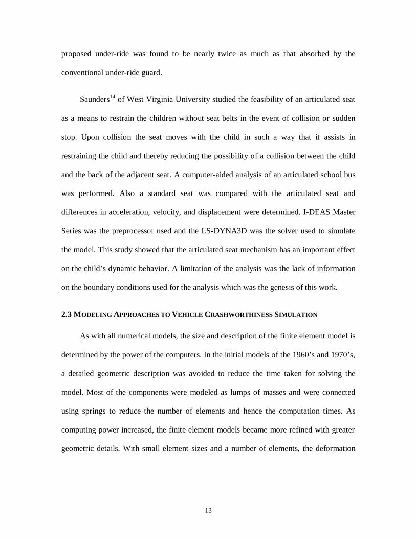
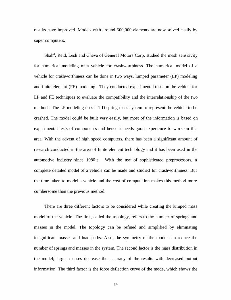
and solving the system to obtain the necessary output. The authors also conducted a mesh

sensitivity study by modeling a rectangular tube using three different meshing

arrangements. Model A had uniform 10x10 mm mesh, whereas models B and C had both

10x10 and 10x15 mm meshes arranged in different patterns. Mild steel properties were

given to the tube. The velocity and the boundary conditions were the same for all the

models; the only difference was the mesh size.

The results are shown in Figure 2.12, which indicates that the mesh size affects the

deformation pattern or the crush kinematics to a considerable extent. In order to obtain a

realistic deformation pattern, the mesh size should be chosen carefully.

16

Fig 2.1 Influence of mesh density on displacement.

Onusic3, Campos and dos Santos of Mercedes-Benz Brazil worked on the

simplified hand calculations of the impact forces during vehicle collisions. There are

many computer programs trying to simulate crash tests, but in order to get an idea about

the magnitude of the impact forces that are to be obtained from the simulation, a hand

calculation can be done using the physical concepts, mechanics, and simplified

17

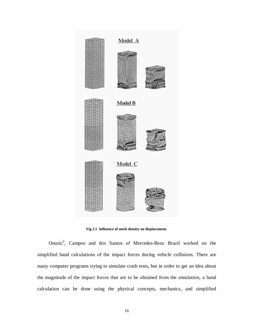
approximations. These collision events are similar to a projectile impact on a rigid wall.

A constant deceleration force is considered and it is assumed that the deceleration force

varies linearly with the time. Cases were considered assuming the vehicle to be extremely

rigid and have a highly inelastic soft body. The effect of the elastic parts such as the

power train was also considered.

The impact is assumed to be equivalent to the deceleration of the vehicle with the

mass at the center of gravity of the vehicle. The basic equations of dynamics give

V2 = V02 – 2ax (2.3.1)

and

V = V0 – at . (2.3.2)

Giving the end conditions V=0, and assuming the vehicle travels for a distance 3

L,

where L is the length of the body, then

L2

V3a

20= . (2.3.3)

For, F = M a, then

L

VM

2

3F

20= . (2.3.4)

18

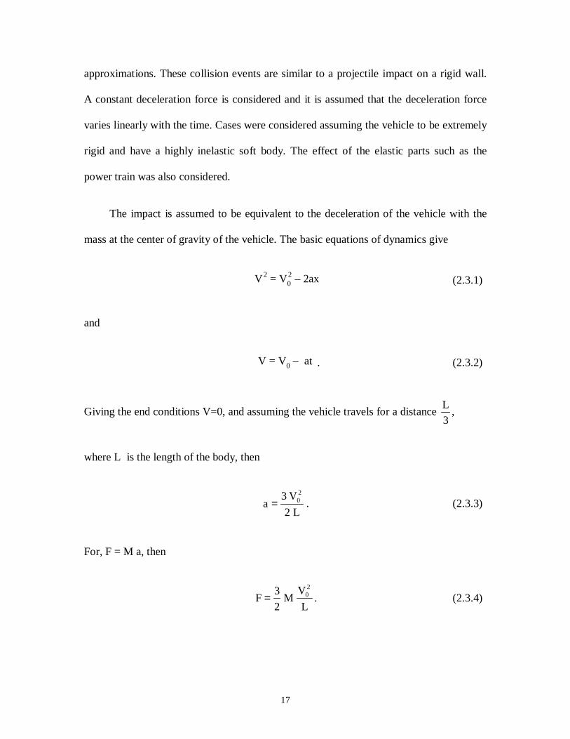
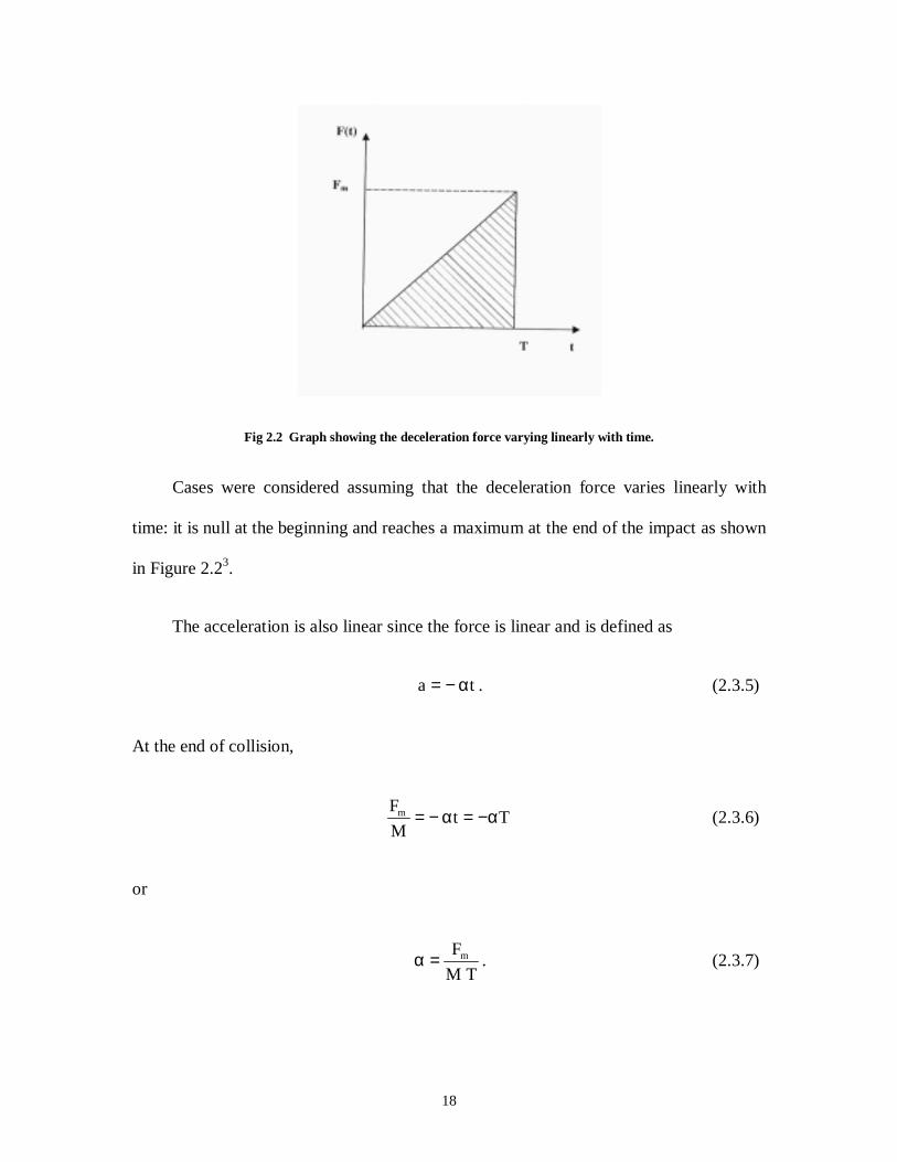
Fig 2.2 Graph showing the deceleration force varying linearly with time.

Cases were considered assuming that the deceleration force varies linearly with

time: it is null at the beginning and reaches a maximum at the end of the impact as shown

in Figure 2.23.

The acceleration is also linear since the force is linear and is defined as

ta α−= . (2.3.5)

At the end of collision,

TtM

Fm α−=α−= (2.3.6)

or

TM

Fm=α . (2.3.7)

19

Integrating the acceleration, the velocity is determined and the constant of integration is

Vo :

2

tVV

2

o α−= . (2.3.8)

Integrating the velocity, the displacement is

6

ttVx

3

o α−= . (2.3.9)

When the center of gravity reaches a zero velocity, V = 0; substituting this back into

equation (2.9) yields

6

tx

3

α−= (2.3.10)

The time taken for impact is given as

α= o2 V

2T . (2.3.11)

The impulse of the force can be calculated from the area under the curve in Figure 2.2

Calculations were also made considering the vehicle as an extremely rigid body and

as an extremely soft body. When the rigid body hits a rigid wall, a shock wave will be

transmitted through its body travelling the length of the body and reflecting back and

forth. The velocity of the shock wave will be equal to the velocity of the sound in the

material. The equation for the impulse force is given by

20

L

VMF oγ= (2.3.12)

where

oV

C=γ . (2.3.13)

When the vehicle is considered as an extremely soft body, it can be imagined as a

bag of fluid. When the vehicle hits the wall, the rear portion of the body doesn’t

experience any load as per this assumption. The mass progressively touches the wall and

spreads on its surface. The shock is perfectly inelastic. The impulse force is given by

L

VMF

2o= . (2.3.14)

The results were applied to a passenger car and a bus, and the results were

underestimated in relation to real data. Also it was observed from the elastic and inelastic

models that the reduction of wave shock preserves the rear parts of the vehicle.

Ingarashi4 of Suzuki Motor Co. performed a body structural analysis of a 1989

Suzuki Sidekick at various stages of development and design. This paper illustrates that

the application of the structural analysis for the body structure along with the experiment

is beneficial if applied at the earlier stages of design. There are three stages in the

development of car body structure. The first stage is to develop a body structure that

satisfies the basic requirements of a car body such as structural rigidity, weight, natural

frequency, and crashworthiness. The second stage studies these factors in more detail and

evaluates these factors; and this stage results in detailed design drawings of the body

21

structure. In the third stage, the results obtained are compared with the experimental

results from a prototype.

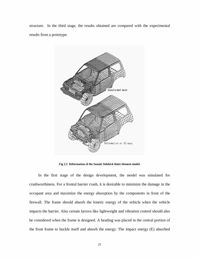
Fig 2.3 Deformation of the Suzuki Sidekick finite element model.

In the first stage of the design development, the model was simulated for

crashworthiness. For a frontal barrier crash, it is desirable to minimize the damage in the

occupant area and maximize the energy absorption by the components in front of the

firewall. The frame should absorb the kinetic energy of the vehicle when the vehicle

impacts the barrier. Also certain factors like lightweight and vibration control should also

be considered when the frame is designed. A beading was placed in the central portion of

the front frame to buckle itself and absorb the energy. The impact energy (E) absorbed

22

can be expressed as a product of the buckling force (F) and the amount of deformation

(D). The buckling force or the amount of deformation is equal to a function f (location of

the beading, gauge thickness, cross section of the frame, shape of the frame). Also a

detailed analysis of front-end components like the bumper was also carried out. The

frame designed for the vehicle was a 3-partitioned frame unlike a conventional one, and

hence the frame had to be tested for its strength and durability. Experiments were carried

out on a similar vehicle and the loads coming on the frame were calculated

experimentally. From then, these loads were applied to the 3-partitioned frame under

development and a finite element analysis was carried out.

A design change in the later stage becomes difficult if the cross sectional details are

not studied in detail in the earlier stages of design. So, at an earlier stage of design, the

basic body structure was modeled by using bar elements to optimize the body structure as

much as possible. The advantages of this simple model are the ease of calculation, ease of

incorporation of changes in design, and reduced time. A skeleton model of a similar

vehicle was created and analyzed and compared with the experimental results to make

sure the design process is moving in the right direction. Once the skeletal model was

checked for the design durability and vibration, a detailed fine grid mesh of the entire

vehicle body was created. Then using the fine grid mesh, the model was checked for

rigidity and vibration to make sure that the structure will not exhibit a resonance with the

disturbance and the exciting force exerted on the body. A crashworthiness simulation was

carried out using the fine grid mesh of the vehicle body for frontal and rear barriers. Only

half of the model was analyzed owing to the symmetry of the model. Rigid elements

were used in places where there are no deformations. The model was given an initial

23

velocity of 35 mph and the calculation was terminated after 100 ms. The experimentally

determined body deceleration and body velocity were compared with the simulation

results and a good correlation was found.

Lugt5, Chen and Deshpande of General Motors Corp worked on the numerical

simulation of a passenger car frontal crash at 48 km/hr (30 mph). The model was solved

in PAM-CRASH, which is an explicit finite element code. In crashworthiness, an

effective design is the one which effectively absorbs the energy required to protect the

occupants and meets all other requirements. The explicit method can take full advantage

of the modern day super computers rather than the implicit method. PAM-CRASH is an

explicit finite element code, which directly yields the nodal accelerations solving the non-

linear equations of motion. This produces a diagonal lumped mass matrix, which can be

solved easily by a computer. The velocities and displacements are obtained from the

nodal accelerations by the central difference method. The size of the integration time step

is a limitation to the explicit method. For the solution to remain stable, the time step must

be smaller than the time it takes for the sound to travel through the smallest element in

the mesh. If this condition is not met, the solution may not converge to the exact solution

and might diverge to a different one. Hence the explicit method is extremely useful for

crash events.

The model of the vehicle was created with a closer mesh density at the front end

where there is large deformation and sparser mesh density at the middle portion of the

vehicle where the deformation would be much less. An increase in the mesh density at

the front end increases the chances of capturing even the smallest buckling in he vehicle.

However the integration time step is controlled by the smallest element in the mesh and

24

hence the cost of computing would also be high. Only the front portion of the vehicle was

modeled and the rear portion was given as a concentrated mass at the appropriate places

to produce the correct center of gravity for the vehicle. The model was solved for 48

km/hr (30mph) and the deformation shapes were obtained. An experimental test was also

conducted; the final deformation shape of the vehicle was compared and a good

agreement between the results was determined.

Belytschko6 of the Civil and Mechanical Engineering Department at Northwestern

University presented the evolution of computers for crashworthiness and the

computational methods available. The improvement in computational methods shows up

as more effective time integration procedures and more efficient elements. In the mid

1970’s the time required for solving a 500 DOF model of a Plymouth car took up to

twenty hours of running time for the solver in the largest mainframe at that time, costing

up to $1000 an hour, though the results of the simulation were comparable with the test

results. The next principal development in the area of crashworthiness was the 4-node

quadrilateral thin shell element, which required only one quadrature per element. This

helped to decrease the time for computation by tenfold. At the same time, a dynamic

analysis code called LS-DYNA3D was developed by Lawrence Livermore National

Laboratory, which used explicit time integration and was completely vectorized to take

advantage of the Cray computer architecture. The only disadvantage with the explicit

method is that a small time step has to be used in order for the solution to be stable. The

time step should be less than the time required for the elastic wave to travel the size of the

smallest element in the model. So if the model has even one small element, the time

required for the entire solution is increased. This was overcome by the multi time step

25

integration. In this method, the elements are divided into groups and a different time step

is used for each group, so that if only one group has small elements, they alone are

integrated with a smaller time step. One of the major improvements in the area of mesh

creation is the adaptive meshing technique. By this method, the mesh is refined during

the course of the computation in order to achieve the desired accuracy.

Piatak8 of ASC Inc., Sheh of Cray Research Inc; and Young and Chen of Optimal

CAE, Inc worked on a convertible crashworthiness design using non-linear finite element

methods. The frontal and rear impacts of the convertible car were studied using the

dynamic non linear finite element code LS-DYNA3D, and the results were verified with

the experimental crash. Most of the vehicles were not designed with the convertible

option in mind, and as a result of the conversion process the vehicle loses its structural

stiffness to a large extent. Convertibles are modified two door coupes with the roof and

the pillar being replaced by a retractable top. Since the pillars are removed, the load path

through the roof structure is affected, and most of the impact is transferred through the

door structure and the lower load path such as frame and rocker. Without proper

reinforcement, during a crash event there might be excessive damage to the doors and

floor and there are chances of impact entering the occupant area.

LS-DYNA3D was used for designing the front structure reinforcement package

design and deck lid crashworthiness. When the actual vehicle was crashed at an impact

velocity of 56 km/hr (35 mph), the test results showed significant deformation of the

front structure leading to inadequate occupant kinematics. The test vehicle was stripped

down to study all the deformations in detail. The poor performance of the vehicle was

attributed to the lack of roof structure. Various alternatives were suggested to overcome

26

the problem, and it would be very costly and time consuming to evaluate all the

suggestions by experiments. To compare the effectiveness of the various reinforcement

scenarios, only the front half of the body was modeled. The model had approximately

28000 nodes, and 27000 shell elements, and 1200 spot welds. A symmetric boundary

condition was defined and a rigid barrier was defined to move at a constant velocity of 56

km/hr (35 mph) impacting the front end of the vehicle. One of the suggestions proposed a

tubular brace between the firewall and front barrier to stabilize the shock tower

deformation. This proposal, when modeled in LS-DYNA3D and analyzed, gave the least

amount of header drop and pillar rotation. When this model was tested experimentally, at

56 km/hr (35 mph) against frontal barrier, the pillar experienced much less deformation.

In addition both the driver and the passenger doors opened easily after the crash, which

helps the passengers to exit.

The deck lid is a new design that covers the trunk opening when the retractable top

sits on the trunk. It is hinged at the rear and latched at the front. In the previous 35 mph

rear impact test, the deck lid was not sufficiently crushed, transmitting a large amount of

forces through the front mounting brackets. The requirement is that the deck lid should sit

on the trunk opening after the rear impact. Various proposals were made and a finite

element model of the deck lid was built consisting of 5500 shell elements and constrained

at three mounting bracket locations. One of the proposals which suggested with two crush

initiators near two front mounting plates and one at the center with thinner and outer

panels behaved better with lesser peak force in crush. Experiments were conducted and

the results compared well with an experimental peak force of 20.5 kN, giving a simulated

force of 19.8 kN.

27

Garrot19 and Flick of NHTSA and Mazzae of Transportation Research Center, Inc.

worked on the comparison of electronics based object detection systems for heavy trucks.

The object detection systems can be classified into two groups: rear object detection

systems and side object detection systems. The rearward sensing systems are intended to

help drivers when they are backing their vehicles at very low speeds in order to avoid

crashes with parked vehicles or pedestrians or other fixed objects. Comparison was made

among six commercially available systems. The side object detection system is used as a

supplement to the outside rearview mirror systems and as a means for detecting adjacent

vehicles when making a lane change or merging maneuvers. Changing lanes towards the

right is a difficult task for drivers in dense traffic situations. Four such systems were

evaluated and compared. Data from National Accident Sampling System shows that in

1991 an estimated 190,000 crashes involved combination unit trucks resulting in 4,849

fatalities, of which 3764 were occupants of other vehicles involved in the crashes and 659

were occupants of the heavy trucks.

From the study, conclusions were made about the rear object detection systems.

Compared to vehicles that are not equipped with these systems, the rear object detection

systems may have the potential to improve safety and reduce accidents while backing. A

rear mounted video camera with microphone helps the driver to see and hear what is

behind the vehicle. The fields of view of the cameras were evaluated and found to be

adequate for most backing situations. The information obtained by the camera is

transmitted to the driver in an easily-understand form. Conclusions were made about the

side object detection systems and these systems may provide benefits to drivers by

greatly increasing the visibility and awareness of the drivers as to what is happening on

28

the lane to the right. Especially in areas of dense traffic, these detection systems may help

the driver to make quick decisions about whether or not it is safe to change lanes. Also,

improvements in these systems are necessary to receive significant benefits.

Rechnitzer and Murray20 of Monash University and Scott of VICROADS Road

Safety Inc. worked on a detailed investigation of the injuries to car occupants in rear end

impacts with heavy vehicles. Also, a demonstration of an effective lightweight

inexpensive barrier on the rear of the vehicle was made that reduced injuries during an

underrun.

The rear underrun is described as the front of a car or any other small vehicle that

follows the truck, sliding under and colliding with the rear end of a truck or trailer. This

underride occurs because the rear end of the truck is high off the ground and there is

nothing to resist the vehicle that strikes the back of the truck in case of an emergency

braking. This type of crash results in a severe injury to the occupants of the smaller

vehicle that hits the truck and in most of the cases the rear end of the truck crashes

through the wind screen and strikes the front passenger compartment. In the United

States, 350 people were killed in underride crashes in 1978. The possible injuries to the

occupants of the car were multiple lacerations on the forehead and face and fractures of

the skull and frontal bones. Also, occupant protection systems like the airbag and the seat

belt are quite ineffective and are more likely to result in direct occupant impact with the

truck structure resulting in severe or fatal head and chest injuries.

To prevent injuries to occupants of cars colliding with the rears of truck; the first

prerequisite is to prevent excessive underrun. The second consideration would be to

29

reduce occupant compartment injuries and to reduce the deceleration of the passenger.

The first prerequisite can be achieved by attaching a barrier of sufficient strength and

appropriate height to the rear of the truck. This barrier should be able to absorb energy

effectively and resist the impact load from the car. In this case, the occupant survivability

becomes a factor of the occupant protection systems like the airbag and the seat belt and

the crashworthiness characteristics of the car. If the barrier is deformable and capable of

absorbing large amounts of energy, then the risk of injuries would be reduced further.

Also the barrier should work effectively if the impact is not only central, but also for side

impacts, in which case the load is not distributed over the full length, but resisted only by

a part of the barrier structure.

It was concluded that the truck without a rear end rigid barrier would cause more

injuries and fatalities to the car that crashes the rear end than a truck that is fitted with a

light weight barrier that could absorb energy and prevent a car underrun. Also it was

concluded that the loads imposed on barriers during the test exceeded the loads stated as

design loads in the proposed United States rules.

Shiosaka21 of Japan automobile research institute investigated the evacuation

readiness of the bus crews and passengers and studied the effect of a new type of exit for

the passengers. The new type of exit was developed based on the results of current bus

exit performance tests. Also, tests were conducted to measure the time required to

evacuate using the improved emergency exit. Group evacuation tests through windows

were carried out to compare the time required to exit in the regular and the new

emergency exits. The new emergency exit aimed at improving the safety for passengers

with diminished physical functions and for aged persons while making an emergency

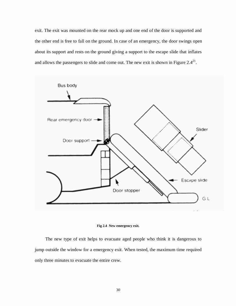
30

exit. The exit was mounted on the rear mock up and one end of the door is supported and

the other end is free to fall on the ground. In case of an emergency, the door swings open

about its support and rests on the ground giving a support to the escape slide that inflates

and allows the passengers to slide and come out. The new exit is shown in Figure 2.421.

Fig 2.4 New emergency exit.

The new type of exit helps to evacuate aged people who think it is dangerous to

jump outside the window for a emergency exit. When tested, the maximum time required

only three minutes to evacuate the entire crew.

31

Kaufman and Gaines22 of Ford motor company, Kundrick of Tower Automotive

Inc., and Sheng-Dong Liu of National Steel Corporation worked on the integration of the

frame side rail forming analysis into the finite element crash model. For vehicles that

have the body on the frame, the chassis truck frame absorbs about 70% of the total

kinetic energy created during the frontal impact. Traditional crash analysis utilizes the

standardized material properties for the finite element model. When these properties are

used, the steel does not reflect any strain hardening effects that occur during the forming

process. The properties from the forming analysis like the material thin out, yield

strength, and tensile strength were input into the crash finite element model of the

vehicle. These properties modified the frame deceleration pulse and buckling mode

characteristics in the crash output.

The frame structure is designed to meet a target stiffness that absorbs kinetic energy

from frontal impact. Despite the efforts of modeling the frame carefully, the model might

not be a complete representation of the vehicle because the raw steel properties assumed

for the frame are not the same as the formed steel properties. When the raw steel

properties are used for the frame in the finite element model, the non linear performance

analysis does not take into account the change in material properties during the forming

process. The flat stock undergoes strain hardening and changes in the yield strength

during the stamping process. A new process was proposed that could use the final

properties of steel in the finite element model.

In the new method of analysis, the starting point remains the same as the existing

process; raw steel material properties are provided to construct a finite element model. A

forming analysis is performed first before any crash analysis is performed. The forming

32

analysis software gives the final shape of the frame, which can be completed in a half

day. Using the same frame model for the forming analysis and the performance analysis

allows for easier implementation of the material properties and it could also lead to the

automation of the forming results into the starting point of the performance analysis.

Upon completion of the forming analysis, the material properties are updated in the finite

element model and the model is transferred to undergo a crash analysis. The strain

hardening in the model, the greater the effect on the yield strength and tensile strength.

The proposed method was implemented on a vehicle CAE program.

The crash finite element model was created and transferred to the steel supplier to

complete the forming analysis. After the forming analysis, a crash analysis was

performed and the results were determined. A standard crash analysis was performed

using the raw steel data and the results were found to differ. The new method agreed

closer to the base line.

Tanner23, Chen, Wiechel, Brown of S.E.A Inc., and Guenther of Ohio State

University studied the effect of low speed rear impacts on the vehicle and the occupants.

A more common type of rear impact is the one in which the bumper of the striking

vehicle rides over or under the rear bumper of the struck vehicle. One example of this

case is the car running under the rear end of a truck. These types of impact cause more

injuries to occupants than the bumper to bumper impacts at identical speeds. Several

kinds of such impacts were tested with Hybrid III dummies or human volunteers.

Three separate vehicle configurations were utilized to perform the crash study. In

the first test series, the striking vehicle was a Kenworth conventional tractor and the

33

struck vehicle was a 1981 Ford Mustang. The front bumper of the Kenworth is mounted

directly on the frame of the vehicle and the rear bumper of the mustang consisted of a bar

mounted to energy absorbers. In the second test series the striking vehicle was a 1982

Plymouth Horizon and the struck vehicle was a 1986 Chevrolet S-10 Blazer 4X2. The

front bumper of the Horizon consisted of a plated aluminum extrusion that mounts on to

energy absorbers that attach to the vehicle frame. The rear bumper of the Blazer is

chrome plated steel attached to the vehicle frame through mounting brackets. In the third

test series, the striking vehicle was a Mack conventional tractor and the struck vehicle

was a 1986 Toyota Camry. The front bumper of the Mack was the same as the Kenworth

in the first series and the rear bumper of the Camry was constructed from a rubber cover

over an energy absorbing structure that mounts on the frame.

Results were obtained for the three series of vehicles. In the first series, the most

important result was that there was no capacity for energy absorption on the front surface

of the Kenworth tractor. Though the rear of the Mustang had an energy absorber, the

speed of the impact was insufficient to cause any significant energy absorption. In the

second test series, the energy absorbers of the Horizon worked as they were designed to

and stroked completely. At a velocity of 12 km/hr (7.5 mph), the energy absorption

capability of the Horizon was overcome and the bumper structure collapsed and rode

under the Blazer bumper which penetrated into the grill and front structure of the

Horizon.

This study gave an opportunity to examine the effect of override and underride on

vehicle impact response at low speeds. Since the impact is over the bumper or under the

bumper, the minimum velocity to cause a damage to the vehicle would decrease. But

34

from the results of the tests conducted, it did not seem to be true. Also, at higher speeds

where the damage is expected to be more, the involvement of the softer vehicle structures

in a crash would result in reduced forces and impact.

Smith and Ravipati13 of West Virginia University worked on the crashworthiness of

a passenger car model subjected to full frontal, offset frontal and pole collision events.

Only front end of the vehicle was modeled to efficiently simulate the front end model for

the majority of collision events. The complete model consisted of 18208 nodes,16463

shell elements, 1243 solid elements, and 8 beam elements. The full frontal collision event

results were compared with the DOT supplied test data for validation. An hour glassing

problem was encountered when the model was solved for frontal impact. When the

kinetic energy, internal energy and the total energy was plotted against time, there was a

sharp increase in the total energy at around 30 ms. When the model was examined at this

point, it was found that the engine came into contact with the core support at this time,

and the average element length in the engine was much larger than the one in the core

support. The element length was reduced to a finer mesh and the solution was run again.

This result showed no abrupt change in the energies. One more way of avoiding this

problem would be to do eight point integration, which may cost more than reducing the

element length. So care should be taken that the ratio of the element lengths of the

contacting faces is not large. Also, the experimental and the simulated energy absorption

during the full frontal collision event matched well and the results were verified.

35

2.4 SOFTWARE PACKAGES FOR VEHICLE CRASHWORTHINESS SIMULATION

I-DEAS Master Series9 is one software package in the area of mechanical computer

aided engineering (MCAE) that could integrate design and analysis. This software

provides a series of applications starting from solid modeling to finite element analysis,

design optimization and testing in the area of CAD, and a series of applications from

solid modeling to master assembly and manufacturing in the area of CAM. These

applications are fully integrated so that one can transfer the model from one module to

another. The I-DEAS Master Series 4 has some advanced features like sketch in path,

sketch in place, and several surfacing options that help to create a solid model easily.

The I-DEAS Master Series has good team engineering capabilities; a model can be

checked into the library of the software, and anyone working on the same group can use

the model for reference and pick out a copy of the model from the library. Also, I-DEAS

is compatible with most other finite element software and it can read a wide range of

geometry translators like IGES, DXF, and other formats. Owing to these excellent

capabilities, this software was chosen for creating the geometric model of the bus.

The I-DEAS Master Series was used as a preprocessor for the finite element model

developed. This software can write an ASCII file that contains the nodal and elemental

data for the model along with the material properties and physical properties. Some

standard translators that could write out a LS-DYNA3D input file can read this universal

file. One such translator is IDEADYN written by Aida12 which could read the universal

files and translate them into LS-DYNA3D input files. The contacts can also be defined

inside the preprocessor (I-DEAS Master Series) by giving dummy faces pressures of

36

specified values to the faces that could potentially come into contact. Rigid walls can be

defined by giving nodal moments, and initial velocities can be given by nodal forces of

magnitude equal to the velocity. These initial conditions given in I-DEAS Master Series

can be translated by IDEADYN to write a LS-DYNA3D input file. Also, the termination

time for the analysis, material properties and rigid wall position vectors can be given at

the time of translation from the universal file to the LS-DYNA3D input file. IDEADYN

can translate beams, thin shells, tetrahedral elements and brick elements from an I-DEAS

universal file to an LS-DYNA3D input file.

LS-TAURUS was the post processor used to analyze the results from LS-DYNA3D

output files after the solution. When the solution phase is finished, LS-DYNA3D writes

down both ASCII and binary files for viewing the deformation, stress etc., and also plots

various graphs for the analysis. LS-TAURUS can read these files and can produce a

graphical output for the deformation and stress contours and also plot various graphs for

solution. LS-TAURUS has three phases of post processing, the graphics and deformation

output phase where the graphic results are post processed, the time history phase where

the nodal and elemental component output is obtained as graphs, and the third phase

called the ASCII phase where it can read and display the ASCII files and plot graphs for

global energy, reaction forces, etc.

Other standard software used for crash analysis of vehicles include LL Dyna3D and

PAMCRASH. These codes use the explicit finite element method for solving the system

of equations. The standard preprocessors for these packages are Hypermesh, Patran, and

ProEngineer, which create the desired geometry, mesh it with the elements and nodes,

and write a input file in the standard format.

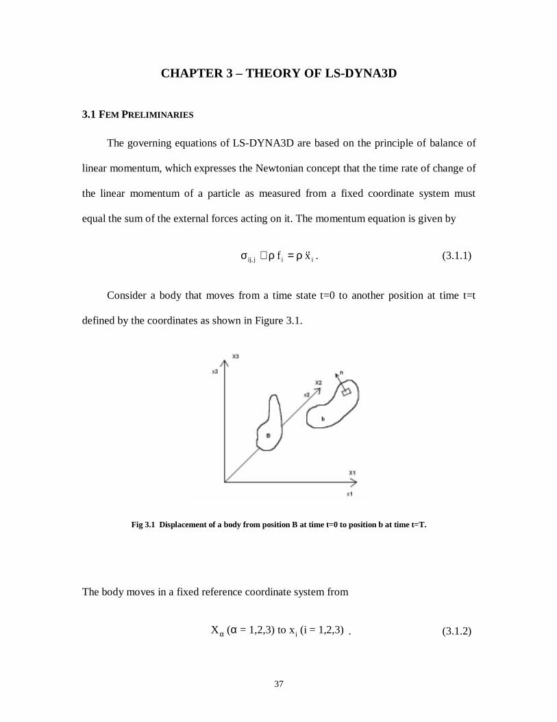
37

CHAPTER 3 – THEORY OF LS-DYNA3D

3.1 FEM PRELIMINARIES

The governing equations of LS-DYNA3D are based on the principle of balance of

linear momentum, which expresses the Newtonian concept that the time rate of change of

the linear momentum of a particle as measured from a fixed coordinate system must

equal the sum of the external forces acting on it. The momentum equation is given by

iij,ij xf &&ρ=ρ+σ . (3.1.1)

Consider a body that moves from a time state t=0 to another position at time t=t

defined by the coordinates as shown in Figure 3.1.

Fig 3.1 Displacement of a body from position B at time t=0 to position b at time t=T.

The body moves in a fixed reference coordinate system from

Xα (α = 1,2,3) to xi (i = 1,2,3) . (3.1.2)

38

The time dependent deformation can be expressed in terms of Xα and t as

xi = xi (Xα,t) , (3.1.3)

based on Lagrangian formulation. The initial conditions describing the body are

xi (Xα,0) = Xα (3.1.4)

and

)X(V)0,X(x ii αα =& . (3.1.5)

The equation of linear momentum is given as

iij,ij xf &&ρ=ρ+σ . (3.1.6)

The traction boundary conditions are given by

t i(t) = σ ij ni . (3.1.7)

The displacement boundary condition over any boundary ∂b1 is

xi(Xα,t) = Di(t) , (3.1.8)

which denotes any final displacement state.

The contact discontinuity over any boundary ∂b2 is given by

(σ ij+ – σ ij

–) n i = 0 . (3.1.9)

39

Forces are balanced over and below the boundary.

Using equations 3.1.6, 3.1.7 and 3.1.9 results in

0dsxn)(dsx)tn(dvx)fx(

21 b

ijijij

b

iijij

v

iij,iji =δσ−σ+δ−σ+δρ−σ−ρ ∫∫∫∂

−+

∂

&& , (3.1.10)

where the integrations are over the current geometry. Applying the Green’s theorem,

which relates the surface and volume integrals,

∫∫∫ δσ=δσ−σ+δσ∂

−+

∂ v

iij

2b

iijij

1b

ijj,ij dvxdsx)(dsxn (3.1.11)

where

(σ ij δxi), j– (σ ij,j δx i) = σ ij δx i,j , (3.1.12)

and a comma denotes a covariant differentiation. Substituting Equation 3.1.11 back into

Equation 3.1.10, yields

∫∫∫∫∂

=δδρ−δσ+δρ=δπ1b

ii

v

ii

v

j,iij

v

ii 0dsxtdvxfdv)x(dvxx&& . (3.1.13)

The above equation gives the statement of principle of virtual work. This is superimposed

over a mesh of finite elements to get the strain displacement matrix.

∑=

α Γηβφ=Γηβ=k

1j

jijii )t(x),,()t),,,(X(xx . (3.1.14)

Summing the same over n elements yields

40

∑=

=δπ=δπn

1mm 0 . (3.1.15)

From equation 3.1.13, the summation for n elements in the model as

∑ ∫ ∫ ∫ ∫= ∂

=φ−φρ−φσ+φρn

1m vm vm vm 1b

mii

mii

mj,i

mij

mii

m

0dstdvfdvdvx&& , (3.1.16)

where

mik321

mi ),...,,( φφφφ=φ . (3.1.17)

3.2 SOLID ELEMENTS

For a mesh of eight noded solid hexahedron elements, Equation 3.1.14 becomes

∑=

αα Γηβφ=Γηβ=8

1j

jijii )t(x),,()t),,,(X(x)t,X(x . (3.2.1)

The shape function φj is defined for the 8-node hexahedron as

ϕ j =1

8(1 + ξξ j) (1 + ηη j) (1 + ζζ j) , (3.2.2)

where ξ j, η j, and ζ j take the nodal values (±1,±1,±1) and xij is the nodal coordinate of

the jth node in the ith direction as per Figure 3.224.

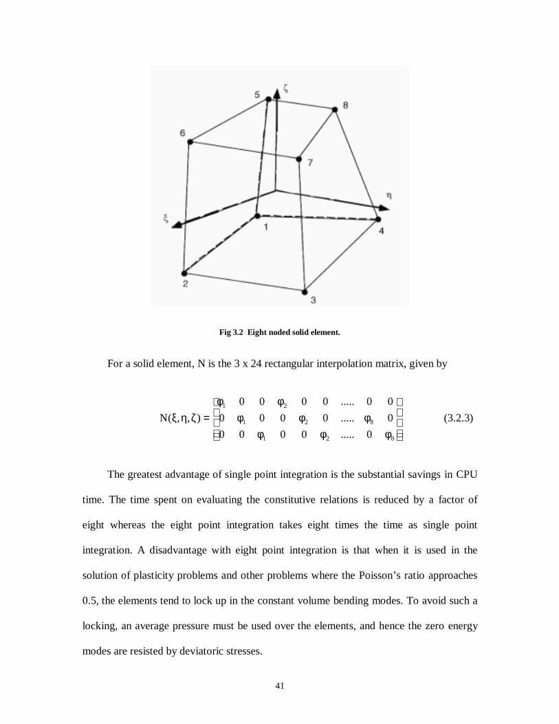
41

Fig 3.2 Eight noded solid element.

For a solid element, N is the 3 x 24 rectangular interpolation matrix, given by

φφφφφφ

φφ=ζηξ

821

821

21

0.....0000

0.....0000

00.....0000

),,(N (3.2.3)

The greatest advantage of single point integration is the substantial savings in CPU

time. The time spent on evaluating the constitutive relations is reduced by a factor of

eight whereas the eight point integration takes eight times the time as single point

integration. A disadvantage with eight point integration is that when it is used in the

solution of plasticity problems and other problems where the Poisson’s ratio approaches

0.5, the elements tend to lock up in the constant volume bending modes. To avoid such a

locking, an average pressure must be used over the elements, and hence the zero energy

modes are resisted by deviatoric stresses.

42

3.3 HOUR GLASS CONTROL

A disadvantage of single point integration is the need to control the zero energy

modes otherwise called the hourglassing modes. These hour glass modes arise when they

have periods that are much shorter than the periods of structural response. The easiest

way of stopping this mode is by giving a small viscous damping or a small resistive

elastic stiffness capable of stopping the modes. The hourglass modes are made

orthogonal to the real deformation and hence the work done by the hourglass modes is

neglected. LS-DYNA3D has three kinds of hourglassing defined in it. Standard LS-

DYNA3D hourglassing takes the least amount of time followed by the Flanagan-

Belytschko hourglassing and Wilkins FDM hourglassing. Table 3.131 shows the

comparison among the methods for the operation count for constant the stress

hexahedron. This includes the additions, subtractions, multiplications, and divisions in

the major subroutine and it is independent of vectorization.

Table 3.1 Operation count for hourglassing types.

Component Standard Flanagan-Belytschko Wilkins FDMStrain displacement matrix 94 357 843

Strain rates 87 156 -Force 117 195 270

Subtotal 298 708 1,113Hourglass control 130 620 680

Total 428 1,328 1,7933.4 TIME INTEGRATION

Consider the single DOF damped system shown in the Figure 3.315. The free body

diagram for the system is shown in Figure 3.415. Applying the D’Alembert’s principle,

the governing equations of the system are written as

43

Fs + FD + FI = p(t) . (3.4.1)

The inertia force can be written as

uMFI &&= , (3.4.2)

where the acceleration is given as

.dt

udu

2

2

=&& (3.4.3)

The damping force is given as

ucFD &= . (3.4.4)

The velocity is

dt

duu =& . (3.4.5)

The force due to the elastic spring is

ukFint = . (3.4.6)

The equations of motion for linear behavior gives the linear O.D.E:

)t(pukucuM =++ &&& . (3.4.7)

The equations for the non-linear behavior give the internal force as a nonlinear

function of the displacement leading to non-linear O.D.E

44

)t(p)u(FucuM I =++ &&& . (3.4.8)

For linear O.D.E closed form solutions are possible but for non-linear O.D.E only

numerical solutions are possible. LS-DYNA3D uses the explicit central time difference

scheme to integrate the equations of motion.

M p(t)

u(t) – displacements

Fig 3.3 Simple spring mass system with a damper.

fI inertia force

elastic force fs

p(t) external forces damping forces fD

Fig 3.4 Free body diagram of the spring mass system.

3.5 CENTRAL DIFFERENCE METHOD

The equations of the motion at any time n are given as

M an = Pn – Fn + Hn. (3.5.1)

To advance to time tn+1, LS-DYNA3D uses the central time integration:

M

)HFP(a

nnnn +−= (3.5.2)

45

The velocity is calculated by

vn + 1 / 2 = vn – 1 / 2 + an ∆ tn(3.5.3)

and the displacement by

un + 1 = un + vn + 1 / 2 ∆ t n + 1 / 2(3.5.4)

where

∆ t n + 1 / 2 =(∆ t n + ∆ t n + 1)

2. (3.5.5)

The variables v and u are the global nodal and velocity and displacement vectors,

respectively. The displacement increments are added to the initial geometry giving

xn+1 = x0 + un+1, (3.5.6)

where x0 is the initial position and xn+1 is the current position.

3.6 NUMERICAL ANALYSIS

Numerical analysis in general attempts to solve the mathematical problems like

differential equations by numerical procedures, which could be programmed using a

standard programming language. The differential equation can be split into numerical

components in the time axis using the forward, central or the backward differentiation

methods and could be programmed to determine the higher time step values from the

initial and boundary values. The numerical methods can be broadly classified as the

explicit and the implicit methods. The explicit method calculates the next time step value

using the previous time step values, whereas the implicit method calculates the next time

46

step values by solving a matrix of the present and the previous time step values. The

explicit method requires shorter time step for an accurate solution, whereas the implicit

methods can give reliable results with larger time steps. Also, most of the implicit

methods are unconditionally stable, whereas the explicit methods are mostly

conditionally stable.

3.6.1 LINEAR AND NON-LINEAR ANALYSIS

A linear analysis assumes that the stiffness matrix in the finite element formulation

is linearly elastic and always obeys Hook’s law. The material properties that are assumed

in this kind of analysis would be infinitely elastic.

A non-linear analysis basically can be classified into two types called the geometric

non-linearity and the material non-linearity. Geometric non-linearity is assumed in the

places where there is a large displacement in the finite element model such as the

deflection in a string or the deflection in a long circular beam where the l/d ratio is very

high. Some finite element packages also take care of the change in the geometry of the

cross section and the shear deflections in this case. Material non-linearity occurs in places

where the material has a finite stress-strain proportionality limit, after which Hook’s law

is no longer valid. In this kind of finite element analysis, the elastic plastic stress-strain

curve is given as an input to the material property of the elements. Once the stress-strain

curve is given as a input to the material property the stiffness matrix is updated

accordingly.

47

3.7 CONTACT IMPACT ALGORITHM IN LS-DYNA3D

LS-DYNA3D has three algorithms for contact defined as the kinematic constraint

method, the penalty method, and the distributed parameter method. The kinematic

constraint method is used only for tying interfaces. Interfaces are defined in three

dimensions; one side of the interface is called the master surface and the other is called

the slave surface. By the kinematic constraint method, constraints are imposed on global

equations by a transformation of the nodal displacement components of the slave nodes

along the contact interface. This transformation has the effect of eliminating the normal

degrees of freedom of the nodes. Impact and release conditions are imposed to insure

momentum conservation. This method has some problems when the master surface is

finer than the slave surface. In this case, the master nodes can penetrate into the slave

surface without resistance. One way to avoid this problem is to have a similar mesh for

the slave surface and the master surface.

The penalty method is used in explicit programs like LS-DYNA2D and LS-

DYNA3D as well as implicit programs like NIKE2D and NIKE3D17. This method

consists of placing normal interface springs between the master and the slave surface.

This method is found to excite if hourglassing occurs and the interface stiffness is chosen

to be approximately the same order of magnitude as the stiffness of the interface element

normal to the interface. If the interface stiffness is too large or too small, penetration may

occur and scaling up and down the penalty stiffness value can solve this problem. This

method increases the number of time steps and the CPU time compared to the previous

method.

48

The distributed parameter formulation involves sharing one half of the slave

element mass of each element in contact to the master surface area. After completing the

distribution of the mass, constraints are imposed on the slave node accelerations and

velocities to ensure their movement along the master surface.

Slave search is common to all the contact algorithms discussed above in LS-

DYNA3D. This search finds the nearest point on the master surface for each slave node.

Lines are drawn from a slave node to the nearest point that will be perpendicular to the

master surface. In contact type 3 in LS-DYNA3D, which is called the sliding with closure

and separation, each slave node is checked for penetration through master surface. If the

slave nodes do not penetrate, nothing is done. If the slave nodes penetrate, an interface

force is applied proportional to the amount of penetration in addition to the interface

stiffness.

Shell thickness can also be taken into account when the contact is defined between

shell elements. This is particularly useful in the case of sheet metal forming operations.

Unless thickness is considered, in the contact, the effect of thinning on fractional

interface stresses due to the membrane stretching will be difficult to treat. For considering

the thickness, the slave and the master surface projections are based from the mid surface

of the shell element. The surfaces, therefore, should be offset by a distance equal to half

the total thickness.

Tied interfaces are useful for joining two meshes of incompatible mesh sizes. This

feature can decrease the effort required to reduce the mesh sizes to match two different

surfaces of different element lengths. In this method the constraints are imposed only on

49

the slave nodes, and it is therefore essential to define the more coarsely meshed side of

the interface as the master surface.

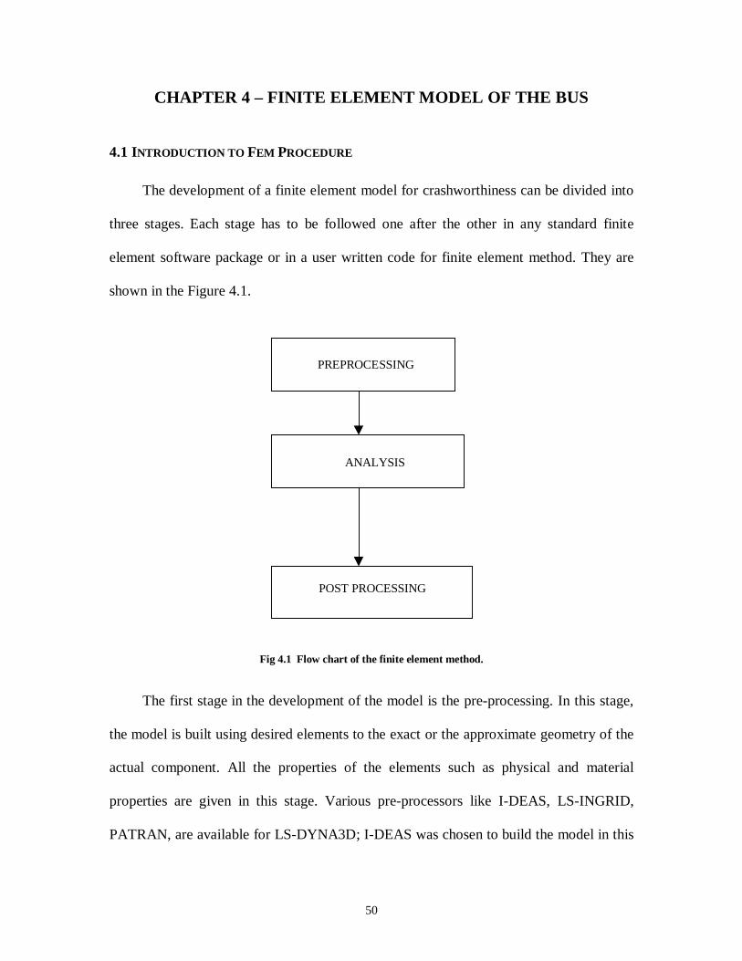
50

CHAPTER 4 – FINITE ELEMENT MODEL OF THE BUS

4.1 INTRODUCTION TO FEM PROCEDURE

The development of a finite element model for crashworthiness can be divided into

three stages. Each stage has to be followed one after the other in any standard finite

element software package or in a user written code for finite element method. They are

shown in the Figure 4.1.

PREPROCESSING

ANALYSIS

POST PROCESSING

Fig 4.1 Flow chart of the finite element method.

The first stage in the development of the model is the pre-processing. In this stage,

the model is built using desired elements to the exact or the approximate geometry of the

actual component. All the properties of the elements such as physical and material

properties are given in this stage. Various pre-processors like I-DEAS, LS-INGRID,

PATRAN, are available for LS-DYNA3D; I-DEAS was chosen to build the model in this

51

case. I-DEAS has excellent capabilities for pre-processing and the model can be

transferred to the LS-DYNA3D input format using standard translators. These translators

read the universal file, translate the data, and write an input file for LS-DYNA3D, which

can be directly submitted for analysis. The physical properties and the material properties

can also be translated from the universal file to the LS-DYNA3D input file.

Once the pre-processing is done, the model is submitted to LS-DYNA3D for

analyzing the model to create the output. The analysis results will be stored as a series of

files and can be given a user-specified name. Most of the files will be in binary format,

and these files contain the results of the analysis and cannot be viewed or understood

without having the software that translates them and gives a graphical output. This stage

is called the post-processing where the standard results like stress, displacement, velocity,

and acceleration are obtained. As in any design or analysis problem, the modeling

strategy may change. From the results in the post processor, the model may have to be

adjusted to meet the experimental or the numerical requirements.

4.2 PRE-PROCESSING

The model of the school bus was built in I-DEAS Master Series 4.0 using various

modules of the software such as Master Modeler, Master Surfacing, Meshing and

Boundary Conditions. The advantage with this software is that the model can be

transferred from one module to the other easily and there are many tools available for

free and mapped meshing.

52

4.2.1 DATA COLLECTION

To start a model for pre-processing, the first step is to measure the geometry of each

component whose finite element model has to be built. The simplest way to get the

dimensions of the component is to get all the component drawings from the company that

manufactures the bus or to get a service manual gives the assembly of the components of

the bus. Drawings were obtained from a manufacturer of a school bus that is used for

student transportation at West Virginia University and thousands of school districts

throughout the United States. Along with the drawings, the measurements of the school

bus were taken by manually measuring each component of the bus using a measuring

tape, Vernier caliper, and a ruler. Also, pictures of various components of the bus and the

assembly of the components were taken with a digital camera and used for assembling

the model.

4.2.2 PRE-PROCESSING IN I-DEAS

Obviously the finite element model of all the components of the bus cannot be

developed due to time constraints and unnecessary usage of resources like memory and

computing time for a non-significant increase in the solution accuracy. The components

that are to be modeled by a finite element mesh must be prioritized. Prioritization was

based on aspects like energy absorbing capability, involvement in the collision event, and

material type.

Table 4.1 shows the prioritization of the components for frontal impact. All the

components listed in Table 4.1 were modeled using I-DEAS. Priority 1 has the highest

priority and Priority 3 the lowest. The rear axle and the body sheet do not play an

important role in the frontal impact and hence they were not considered for prioritization.

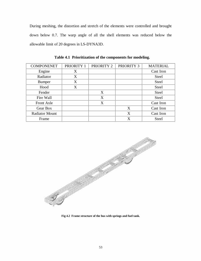
53

During meshing, the distortion and stretch of the elements were controlled and brought

down below 0.7. The warp angle of all the shell elements was reduced below the

allowable limit of 20 degrees in LS-DYNA3D.

Table 4.1 Prioritization of the components for modeling.

COMPONENET PRIORITY 1 PRIORITY 2 PRIORITY 3 MATERIALEngine X Cast Iron

Radiator X SteelBumper X SteelHood X Steel

Fender X SteelFire Wall X Steel

Front Axle X Cast IronGear Box X Cast Iron

Radiator Mount X Cast IronFrame X Steel

Fig 4.2 Frame structure of the bus with springs and fuel tank.

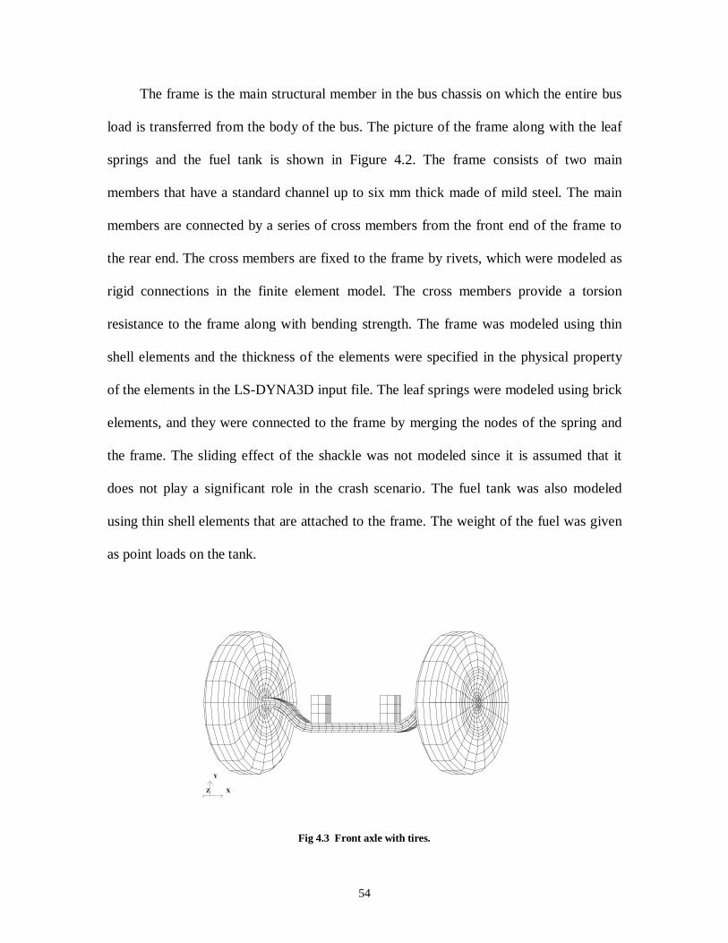
54

The frame is the main structural member in the bus chassis on which the entire bus

load is transferred from the body of the bus. The picture of the frame along with the leaf

springs and the fuel tank is shown in Figure 4.2. The frame consists of two main

members that have a standard channel up to six mm thick made of mild steel. The main

members are connected by a series of cross members from the front end of the frame to

the rear end. The cross members are fixed to the frame by rivets, which were modeled as

rigid connections in the finite element model. The cross members provide a torsion

resistance to the frame along with bending strength. The frame was modeled using thin

shell elements and the thickness of the elements were specified in the physical property

of the elements in the LS-DYNA3D input file. The leaf springs were modeled using brick

elements, and they were connected to the frame by merging the nodes of the spring and

the frame. The sliding effect of the shackle was not modeled since it is assumed that it

does not play a significant role in the crash scenario. The fuel tank was also modeled

using thin shell elements that are attached to the frame. The weight of the fuel was given

as point loads on the tank.

X

Y

Z

Fig 4.3 Front axle with tires.

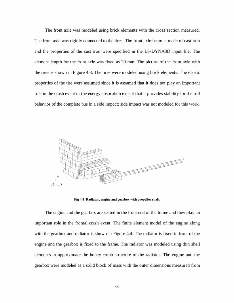
55

The front axle was modeled using brick elements with the cross section measured.

The front axle was rigidly connected to the tires. The front axle beam is made of cast iron

and the properties of the cast iron were specified in the LS-DYNA3D input file. The

element length for the front axle was fixed as 20 mm. The picture of the front axle with

the tires is shown in Figure 4.3. The tires were modeled using brick elements. The elastic

properties of the tire were assumed since it is assumed that it does not play an important

role in the crash event or the energy absorption except that it provides stability for the roll

behavior of the complete bus in a side impact; side impact was not modeled for this work.

X

Y

Z

Fig 4.4 Radiator, engine and gearbox with propeller shaft.

The engine and the gearbox are seated in the front end of the frame and they play an

important role in the frontal crash event. The finite element model of the engine along

with the gearbox and radiator is shown in Figure 4.4. The radiator is fixed in front of the

engine and the gearbox is fixed to the frame. The radiator was modeled using thin shell

elements to approximate the honey comb structure of the radiator. The engine and the

gearbox were modeled as a solid block of mass with the outer dimensions measured from

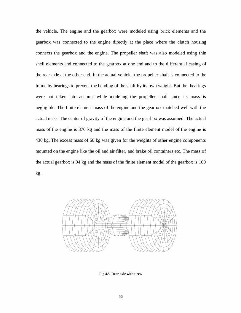
56

the vehicle. The engine and the gearbox were modeled using brick elements and the

gearbox was connected to the engine directly at the place where the clutch housing

connects the gearbox and the engine. The propeller shaft was also modeled using thin

shell elements and connected to the gearbox at one end and to the differential casing of

the rear axle at the other end. In the actual vehicle, the propeller shaft is connected to the

frame by bearings to prevent the bending of the shaft by its own weight. But the bearings

were not taken into account while modeling the propeller shaft since its mass is

negligible. The finite element mass of the engine and the gearbox matched well with the

actual mass. The center of gravity of the engine and the gearbox was assumed. The actual

mass of the engine is 370 kg and the mass of the finite element model of the engine is

430 kg. The excess mass of 60 kg was given for the weights of other engine components

mounted on the engine like the oil and air filter, and brake oil containers etc. The mass of

the actual gearbox is 94 kg and the mass of the finite element model of the gearbox is 100

kg.

Fig 4.5 Rear axle with tires.

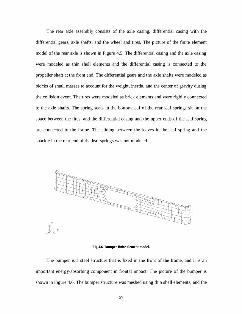
57

The rear axle assembly consists of the axle casing, differential casing with the

differential gears, axle shafts, and the wheel and tires. The picture of the finite element

model of the rear axle is shown in Figure 4.5. The differential casing and the axle casing

were modeled as thin shell elements and the differential casing is connected to the

propeller shaft at the front end. The differential gears and the axle shafts were modeled as

blocks of small masses to account for the weight, inertia, and the center of gravity during

the collision event. The tires were modeled as brick elements and were rigidly connected

to the axle shafts. The spring seats in the bottom leaf of the rear leaf springs sit on the

space between the tires, and the differential casing and the upper ends of the leaf spring

are connected to the frame. The sliding between the leaves in the leaf spring and the

shackle in the rear end of the leaf springs was not modeled.

X

Y

Z

Fig 4.6 Bumper finite element model.

The bumper is a steel structure that is fixed in the front of the frame, and it is an

important energy-absorbing component in frontal impact. The picture of the bumper is

shown in Figure 4.6. The bumper structure was meshed using thin shell elements, and the

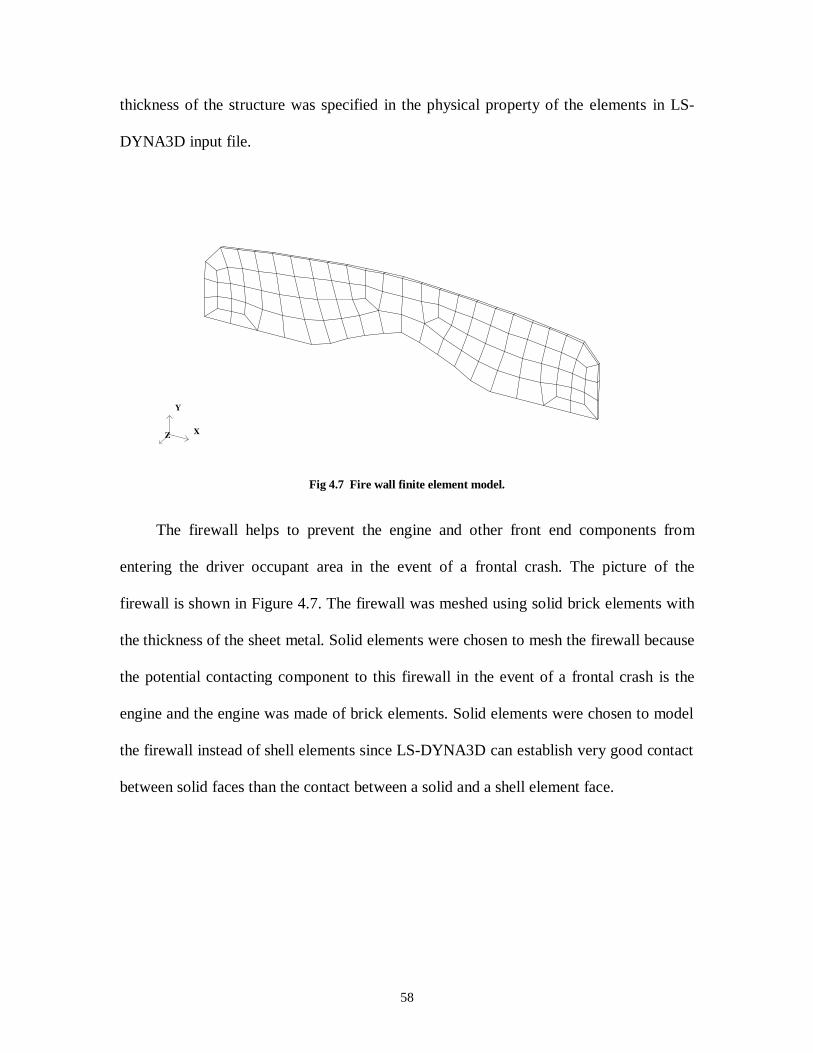
58

thickness of the structure was specified in the physical property of the elements in LS-

DYNA3D input file.

X

Y

Z

Fig 4.7 Fire wall finite element model.

The firewall helps to prevent the engine and other front end components from

entering the driver occupant area in the event of a frontal crash. The picture of the

firewall is shown in Figure 4.7. The firewall was meshed using solid brick elements with

the thickness of the sheet metal. Solid elements were chosen to mesh the firewall because

the potential contacting component to this firewall in the event of a frontal crash is the

engine and the engine was made of brick elements. Solid elements were chosen to model

the firewall instead of shell elements since LS-DYNA3D can establish very good contact

between solid faces than the contact between a solid and a shell element face.

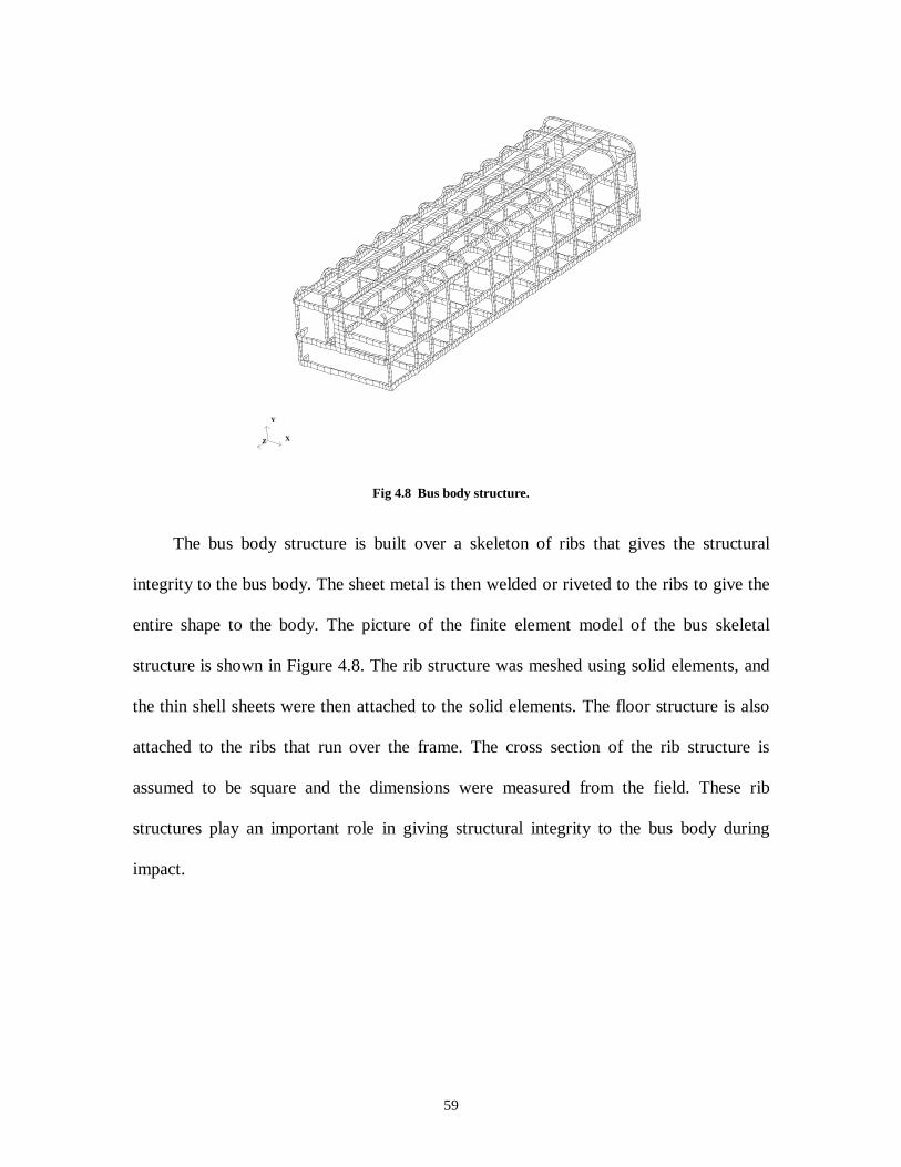
59

X

Y

Z

Fig 4.8 Bus body structure.

The bus body structure is built over a skeleton of ribs that gives the structural

integrity to the bus body. The sheet metal is then welded or riveted to the ribs to give the

entire shape to the body. The picture of the finite element model of the bus skeletal

structure is shown in Figure 4.8. The rib structure was meshed using solid elements, and

the thin shell sheets were then attached to the solid elements. The floor structure is also

attached to the ribs that run over the frame. The cross section of the rib structure is

assumed to be square and the dimensions were measured from the field. These rib

structures play an important role in giving structural integrity to the bus body during

impact.

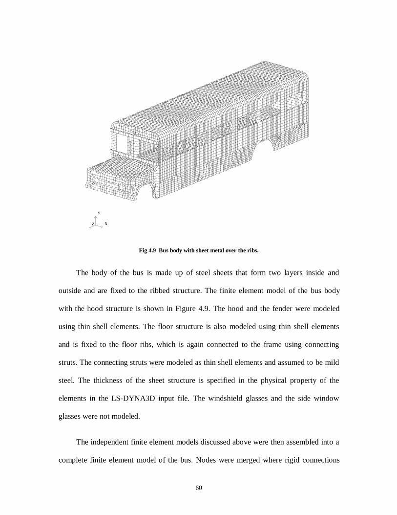
60

X

Y

Z

Fig 4.9 Bus body with sheet metal over the ribs.

The body of the bus is made up of steel sheets that form two layers inside and

outside and are fixed to the ribbed structure. The finite element model of the bus body

with the hood structure is shown in Figure 4.9. The hood and the fender were modeled

using thin shell elements. The floor structure is also modeled using thin shell elements

and is fixed to the floor ribs, which is again connected to the frame using connecting

struts. The connecting struts were modeled as thin shell elements and assumed to be mild

steel. The thickness of the sheet structure is specified in the physical property of the

elements in the LS-DYNA3D input file. The windshield glasses and the side window

glasses were not modeled.

The independent finite element models discussed above were then assembled into a

complete finite element model of the bus. Nodes were merged where rigid connections

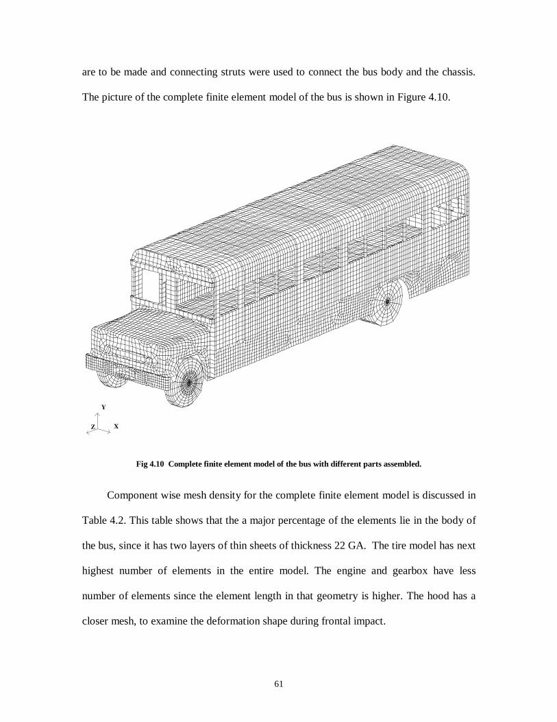
61

are to be made and connecting struts were used to connect the bus body and the chassis.

The picture of the complete finite element model of the bus is shown in Figure 4.10.

X

Y

Z

Fig 4.10 Complete finite element model of the bus with different parts assembled.

Component wise mesh density for the complete finite element model is discussed in

Table 4.2. This table shows that the a major percentage of the elements lie in the body of

the bus, since it has two layers of thin sheets of thickness 22 GA. The tire model has next

highest number of elements in the entire model. The engine and gearbox have less

number of elements since the element length in that geometry is higher. The hood has a

closer mesh, to examine the deformation shape during frontal impact.

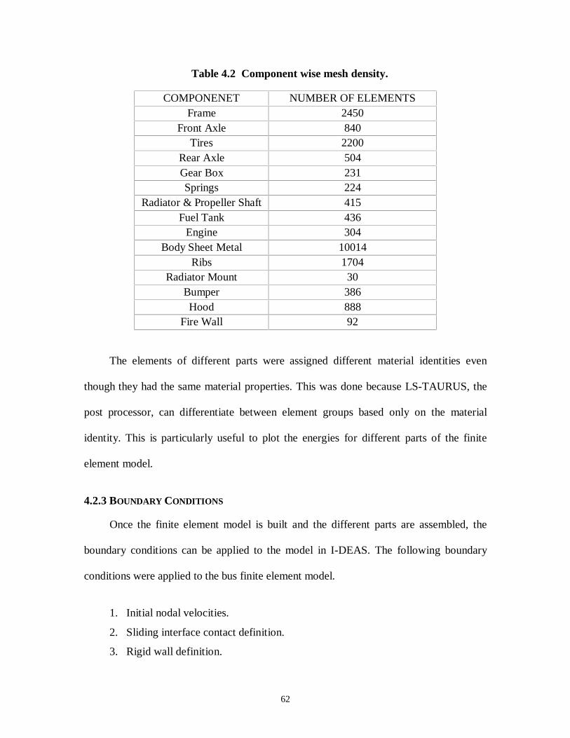
62

Table 4.2 Component wise mesh density.

COMPONENET NUMBER OF ELEMENTSFrame 2450

Front Axle 840Tires 2200

Rear Axle 504Gear Box 231Springs 224

Radiator & Propeller Shaft 415Fuel Tank 436

Engine 304Body Sheet Metal 10014

Ribs 1704Radiator Mount 30

Bumper 386Hood 888

Fire Wall 92

The elements of different parts were assigned different material identities even

though they had the same material properties. This was done because LS-TAURUS, the

post processor, can differentiate between element groups based only on the material

identity. This is particularly useful to plot the energies for different parts of the finite

element model.

4.2.3 BOUNDARY CONDITIONS

Once the finite element model is built and the different parts are assembled, the

boundary conditions can be applied to the model in I-DEAS. The following boundary

conditions were applied to the bus finite element model.

1. Initial nodal velocities.

2. Sliding interface contact definition.

3. Rigid wall definition.

63

I-DEAS does not have a provision for writing the boundary conditions for LS-

DYNA3D. The translator IDEADYN was used to translate the universal file written from

I-DEAS to LS-DYNA3D input deck. IDEADYN is a FORTRAN program that reads the

universal file and writes the nodal data, elemental data, boundary conditions, and the

initial conditions in the formatted input type of LS-DYNA3D. The nodal velocity, which

was the initial condition, was given as nodal forces of magnitude equal to the initial

velocity to all the nodes in I-DEAS. When the universal file is written, IDEADYN reads

the nodal forces and converts them as initial conditions for the nodes in the LS-DYNA3D

input program. The rigid walls are defined for nodes and are given as nodal moments in

I-DEAS. IDEADYN reads the nodal moments from the universal file and writes them as

the nodes that come into contact with a rigid wall in the LS-DYNA3D input file. A rigid

wall definition means the nodes that are defined for the rigid wall are the slave nodes and

the rigid wall is the master surface. That means that the nodes that are defined for the

rigid wall contact cannot penetrate into the rigid wall. By varying the magnitude of the

dummy nodal moments, up to 20 rigid walls can be defined using IDEADYN. The head

and the tail of the normal vector for the rigid wall can be defined during the translation

process.

Contact type 3 in LS-DYNA3D, called the sliding and general interface contact was

defined in the front end of the vehicle. It is defined as face pressures in I-DEAS and the

translator writes them into the LS-DYNA3D input deck. The master surfaces are defined

with a positive force and the slave surfaces are defined with negative forces. Care should

be taken that the shell element normals are oriented in the correct direction for all the

elements. By varying the magnitude of the dummy face pressures, up to 11 contact types

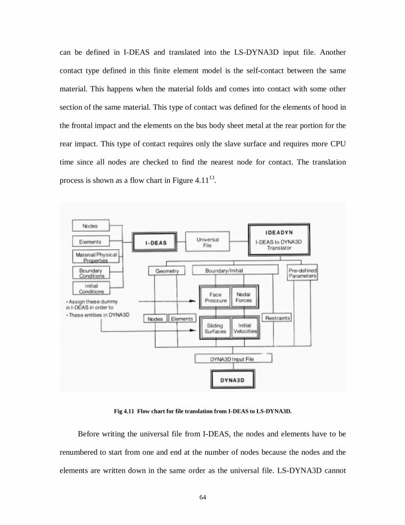
64

can be defined in I-DEAS and translated into the LS-DYNA3D input file. Another

contact type defined in this finite element model is the self-contact between the same

material. This happens when the material folds and comes into contact with some other

section of the same material. This type of contact was defined for the elements of hood in

the frontal impact and the elements on the bus body sheet metal at the rear portion for the

rear impact. This type of contact requires only the slave surface and requires more CPU

time since all nodes are checked to find the nearest node for contact. The translation

process is shown as a flow chart in Figure 4.1113.

Fig 4.11 Flow chart for file translation from I-DEAS to LS-DYNA3D.

Before writing the universal file from I-DEAS, the nodes and elements have to be

renumbered to start from one and end at the number of nodes because the nodes and the

elements are written down in the same order as the universal file. LS-DYNA3D cannot

65

understand if the nodes and the elements are written down in an arbitrary order. This

process is done in the meshing module of I-DEAS, where the elements and the nodes are

renumbered starting from one to the maximum number of nodes or elements.

4.3 ANALYSIS

The analysis of the bus model was performed in LS-DYNA3D. LS-DYNA3D is a

completely vectorized code, which could perform transient nonlinear dynamic analysis of

finite element models. The memory allocation is dynamic and it has several material

types that can be defined for modeling. The limiting factor for the allocation of memory

for the number elements, nodes, boundary conditions, and initial conditions is the

memory of the computer. The interactive execution for this program in the command

prompt is as follows:

LS-DYNA3D I=input file O=output file F=thf.

where I is the user specified input file, O is the output file and F is the time history file.

Similarly, a number of output files can be specified for output. Unless specified, the

default file for the error messages is taken as “messag”. Any kind of errors encountered

during the solution run is written down in this ASCII file and can be viewed. The status

of the solution can be known by using the control switches in the software. Table 4.3 lists

the control switches available and their functions. Two UNIX DEC Alphas, one with 064

chip, 289 MHz, 256 MB RAM and the other with 164 chip, 500 MHz, 1000 MB Ram

were used to solve the finite element models in LS-DYNA3D. LS-DYNA3D version

940.1 was used on both the computers.

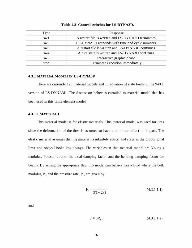
66

Table 4.3 Control switches for LS-DYNA3D.

Type Responsesw1 A restart file is written and LS-DYNA3D terminates.sw2 LS-DYNA3D responds with time and cycle numbers.sw3 A restart file is written and LS-DYNA3D continues.sw4 A plot state is written and LS-DYNA3D continues.sw5 Interactive graphic phase.stop Terminate execution immediately.

4.3.1 MATERIAL MODELS IN LS-DYNA3D

There are currently 126 material models and 11 equation of state forms in the 940.1

version of LS-DYNA3D. The discussion below is curtailed to material model that has

been used in this finite element model.

4.3.1.1 MATERIAL 1

This material model is for elastic materials. This material model was used for tires

since the deformation of the tires is assumed to have a minimum effect on impact. The

elastic material assumes that the material is infinitely elastic and stays in the proportional

limit and obeys Hooks law always. The variables in this material model are Young’s

modulus, Poisson’s ratio, the axial damping factor and the bending damping factor for

beams. By setting the appropriate flag, this model can behave like a fluid where the bulk

modulus, K, and the pressure rate, p& , are given by

)v21(3

EK

−= (4.3.1.1.1)

and

iiKp ε=& . (4.3.1.1.2)

67

4.4 POST-PROCESSING

4.4.1 LS-TAURUS

LS-TAURUS is the post processor for DYNA3D, NIKE3D, and TOPAZ3D. It

reads the binary files written by these packages and plots contours, time histories,

deformed shapes etc., Various nodal data like acceleration, velocity, displacement and

elemental data like the stress and strain can be plotted. Also the strain energies, internal

energies, and kinetic energies for each material can be plotted.

The software is divided into three phases. The first phase can give graphic

information like the stress contours, deformation, and displacement in various modes like

the shaded image or the line image etc. The second phase is for time history plotting. It

can plot various nodal and elemental data. The displacement, velocity, and acceleration

can be plotted for nodes against time and the elemental stress and strains can be plotted

against time. Also material energies can be plotted individually for different materials.

The difference between the values for each nodal component for two nodes can also

plotted. The third phase called the ASCII plotting phase can read the ASCII data files

written by the DYNA3D code. It can read the ASCII file and plot global data, nodal data,

elemental data, rigid wall forces, cross section forces, and the interface forces. Post

processing can be done in parallel to the simulation run. While the solution is going on in

LS-DYNA3D, the results obtained before the completed time state can be post processed.

The file organization for LS-TAURUS is as shown in Figure 4.12.

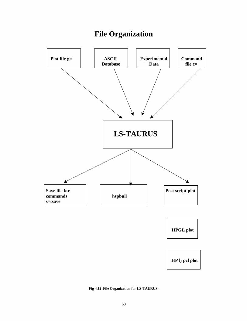
68

File Organization

Plot file g= ASCII Experimental Command Database Data file c=

LS-TAURUS

Save file for Post script plot commands hspbull s=tsave

HPGL plot

HP lj pcl plot

Fig 4.12 File Organization for LS-TAURUS.

69

CHAPTER 5 - RESULTS AND DISCUSSION

5.1 INTRODUCTION

The results of the crashworthiness analysis of the school bus are illustrated in this

chapter. The results include deformation and time history plots for displacement,

velocity, acceleration, and energy. The post processing was done in LS-TAURUS, which

can read the binary and the ASCII files written as output from LS-DYNA3D. The results

can be classified into two types: the macroscopic results like the global values of energy,

velocity, and acceleration and the microscopic information like the displacement,

velocity, and acceleration. The entire time of the crash event is divided into 100 time

states for the ease of post processing, and each state has all the output information at a

specific time of the event. The numerical time step is calculated as illustrated in Section

3.4. The numerical time step is the time taken by the software to move the object from a

position xn to a position xn+1 while the solution is going on. The plot state time step is the

time at which the microscopic and the macroscopic output are written by the software.

Shading and wire frame options, animation options, fringe and contour plots, and vector

displays were used to study and compare the deformation between different components

of the bus model at different time states. Two types of crash analyses were performed on

the school bus model.

• A full frontal rigid wall impact to simulate impact against a wall.

• An offset frontal rigid wall impact to simulate impact against a corner wall.

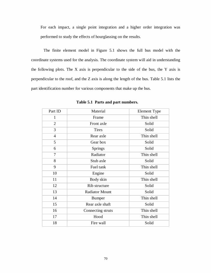
70

For each impact, a single point integration and a higher order integration was

performed to study the effects of hourglassing on the results.

The finite element model in Figure 5.1 shows the full bus model with the

coordinate systems used for the analysis. The coordinate system will aid in understanding

the following plots. The X axis is perpendicular to the side of the bus, the Y axis is

perpendicular to the roof, and the Z axis is along the length of the bus. Table 5.1 lists the

part identification number for various components that make up the bus.

Table 5.1 Parts and part numbers.

Part ID Material Element Type

1 Frame Thin shell

2 Front axle Solid

3 Tires Solid

4 Rear axle Thin shell

5 Gear box Solid

6 Springs Solid

7 Radiator Thin shell

8 Stub axle Solid

9 Fuel tank Thin shell

10 Engine Solid

11 Body skin Thin shell

12 Rib structure Solid

13 Radiator Mount Solid

14 Bumper Thin shell

15 Rear axle shaft Solid

16 Connecting struts Thin shell

17 Hood Thin shell

18 Fire wall Solid

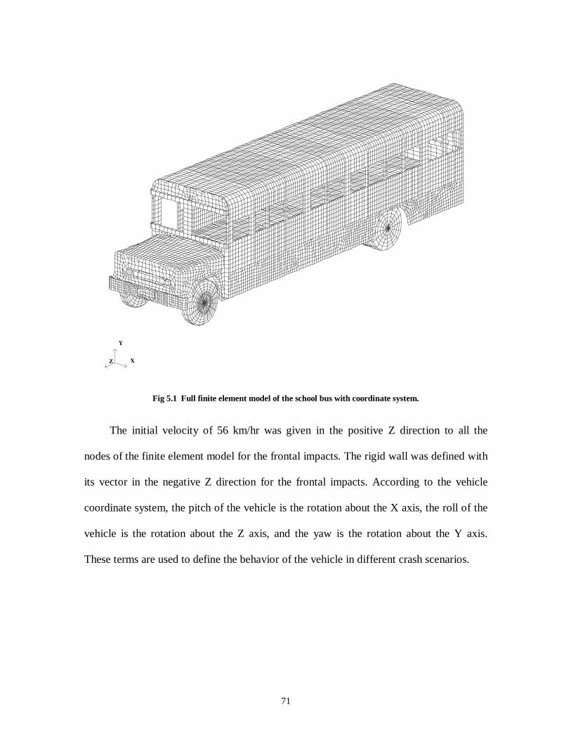
71

X

Y

Z

Fig 5.1 Full finite element model of the school bus with coordinate system.

The initial velocity of 56 km/hr was given in the positive Z direction to all the

nodes of the finite element model for the frontal impacts. The rigid wall was defined with

its vector in the negative Z direction for the frontal impacts. According to the vehicle

coordinate system, the pitch of the vehicle is the rotation about the X axis, the roll of the

vehicle is the rotation about the Z axis, and the yaw is the rotation about the Y axis.

These terms are used to define the behavior of the vehicle in different crash scenarios.

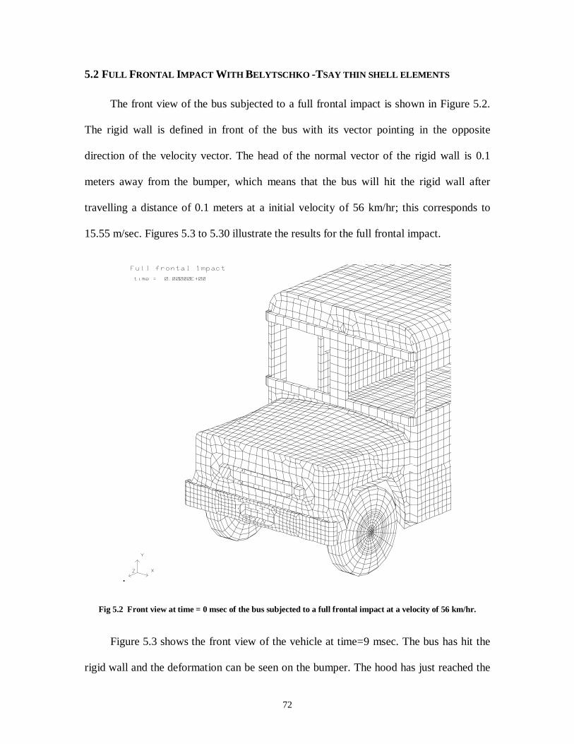
72

5.2 FULL FRONTAL IMPACT WITH BELYTSCHKO -TSAY THIN SHELL ELEMENTS

The front view of the bus subjected to a full frontal impact is shown in Figure 5.2.

The rigid wall is defined in front of the bus with its vector pointing in the opposite

direction of the velocity vector. The head of the normal vector of the rigid wall is 0.1

meters away from the bumper, which means that the bus will hit the rigid wall after

travelling a distance of 0.1 meters at a initial velocity of 56 km/hr; this corresponds to

15.55 m/sec. Figures 5.3 to 5.30 illustrate the results for the full frontal impact.

.

Fig 5.2 Front view at time = 0 msec of the bus subjected to a full frontal impact at a velocity of 56 km/hr.

Figure 5.3 shows the front view of the vehicle at time=9 msec. The bus has hit the

rigid wall and the deformation can be seen on the bumper. The hood has just reached the

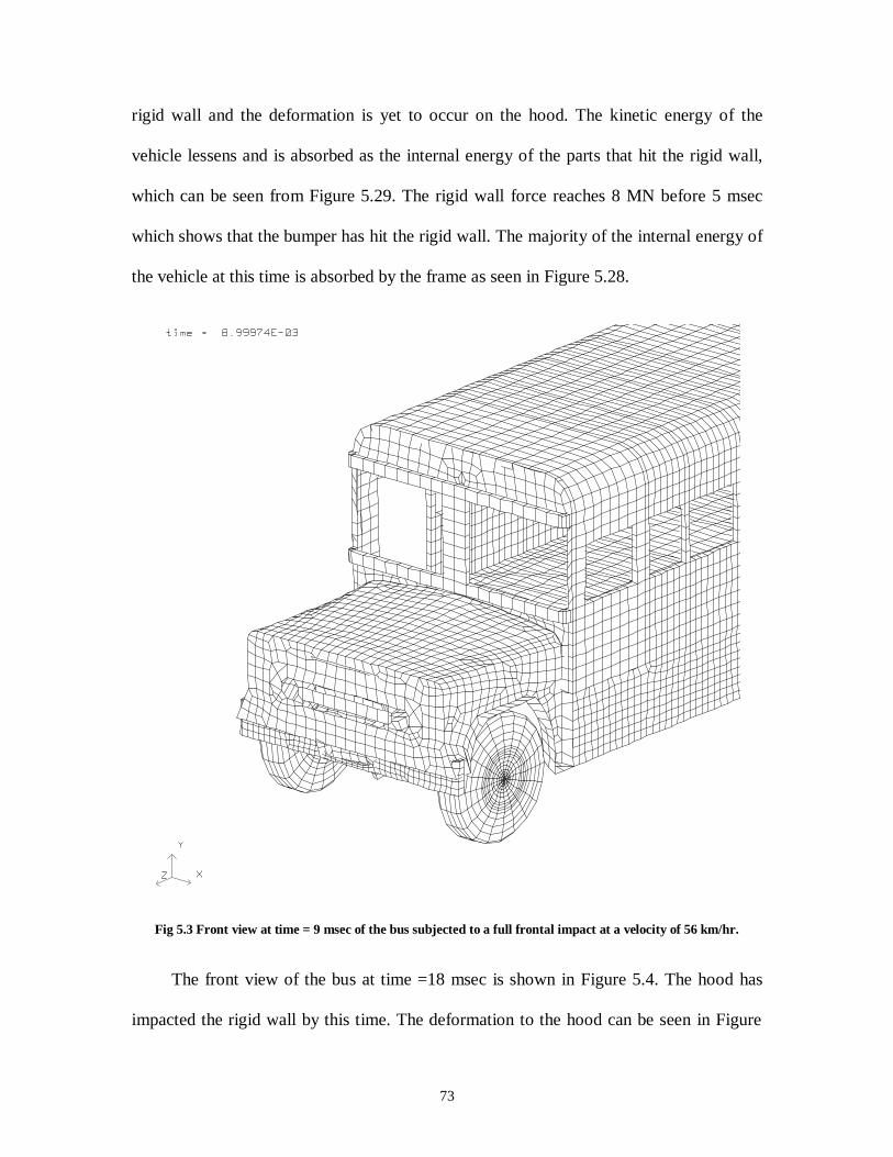
73

rigid wall and the deformation is yet to occur on the hood. The kinetic energy of the

vehicle lessens and is absorbed as the internal energy of the parts that hit the rigid wall,

which can be seen from Figure 5.29. The rigid wall force reaches 8 MN before 5 msec

which shows that the bumper has hit the rigid wall. The majority of the internal energy of

the vehicle at this time is absorbed by the frame as seen in Figure 5.28.


The front view of the bus at time =18 msec is shown in Figure 5.4. The hood has

impacted the rigid wall by this time. The deformation to the hood can be seen in Figure

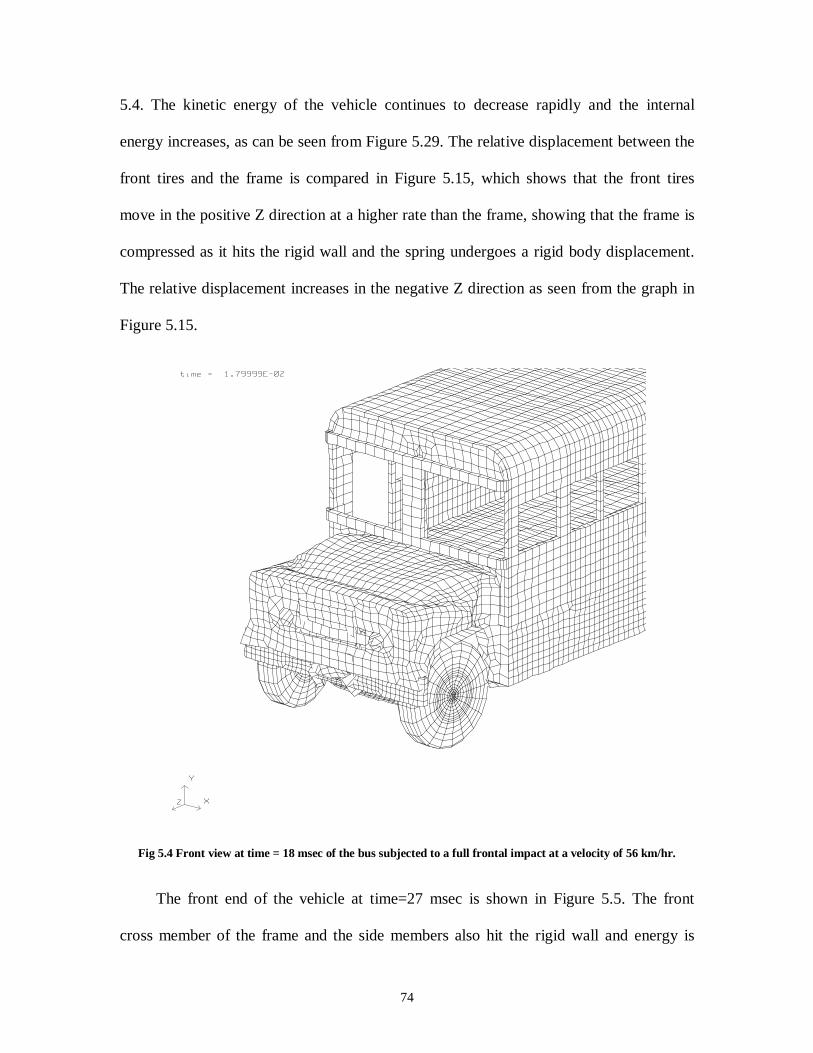
74

5.4. The kinetic energy of the vehicle continues to decrease rapidly and the internal

energy increases, as can be seen from Figure 5.29. The relative displacement between the

front tires and the frame is compared in Figure 5.15, which shows that the front tires

move in the positive Z direction at a higher rate than the frame, showing that the frame is

compressed as it hits the rigid wall and the spring undergoes a rigid body displacement.

The relative displacement increases in the negative Z direction as seen from the graph in

Figure 5.15.


The front end of the vehicle at time=27 msec is shown in Figure 5.5. The front

cross member of the frame and the side members also hit the rigid wall and energy is

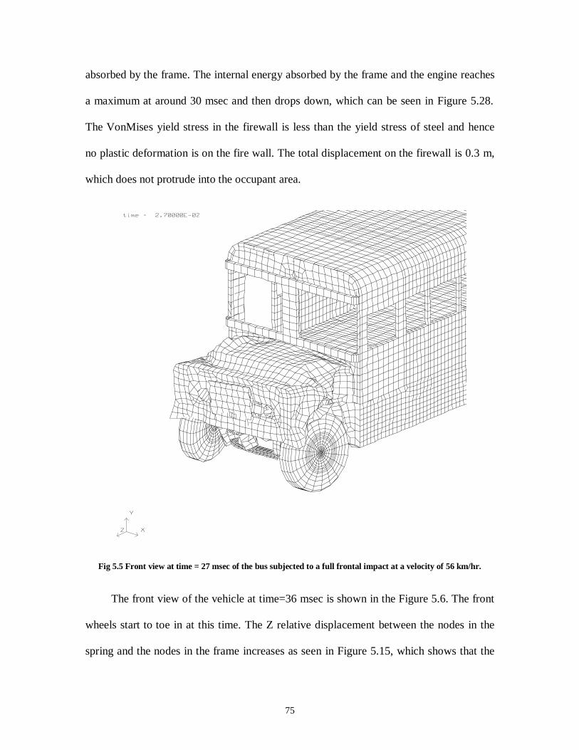
75

absorbed by the frame. The internal energy absorbed by the frame and the engine reaches

a maximum at around 30 msec and then drops down, which can be seen in Figure 5.28.

The VonMises yield stress in the firewall is less than the yield stress of steel and hence

no plastic deformation is on the fire wall. The total displacement on the firewall is 0.3 m,

which does not protrude into the occupant area.


The front view of the vehicle at time=36 msec is shown in the Figure 5.6. The front

wheels start to toe in at this time. The Z relative displacement between the nodes in the

spring and the nodes in the frame increases as seen in Figure 5.15, which shows that the

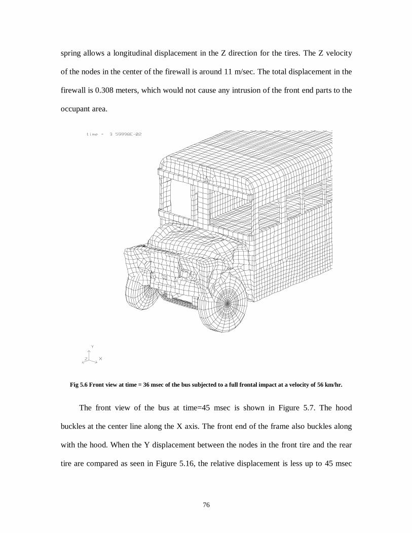
76

spring allows a longitudinal displacement in the Z direction for the tires. The Z velocity

of the nodes in the center of the firewall is around 11 m/sec. The total displacement in the

firewall is 0.308 meters, which would not cause any intrusion of the front end parts to the

occupant area.


The front view of the bus at time=45 msec is shown in Figure 5.7. The hood

buckles at the center line along the X axis. The front end of the frame also buckles along

with the hood. When the Y displacement between the nodes in the front tire and the rear

tire are compared as seen in Figure 5.16, the relative displacement is less up to 45 msec

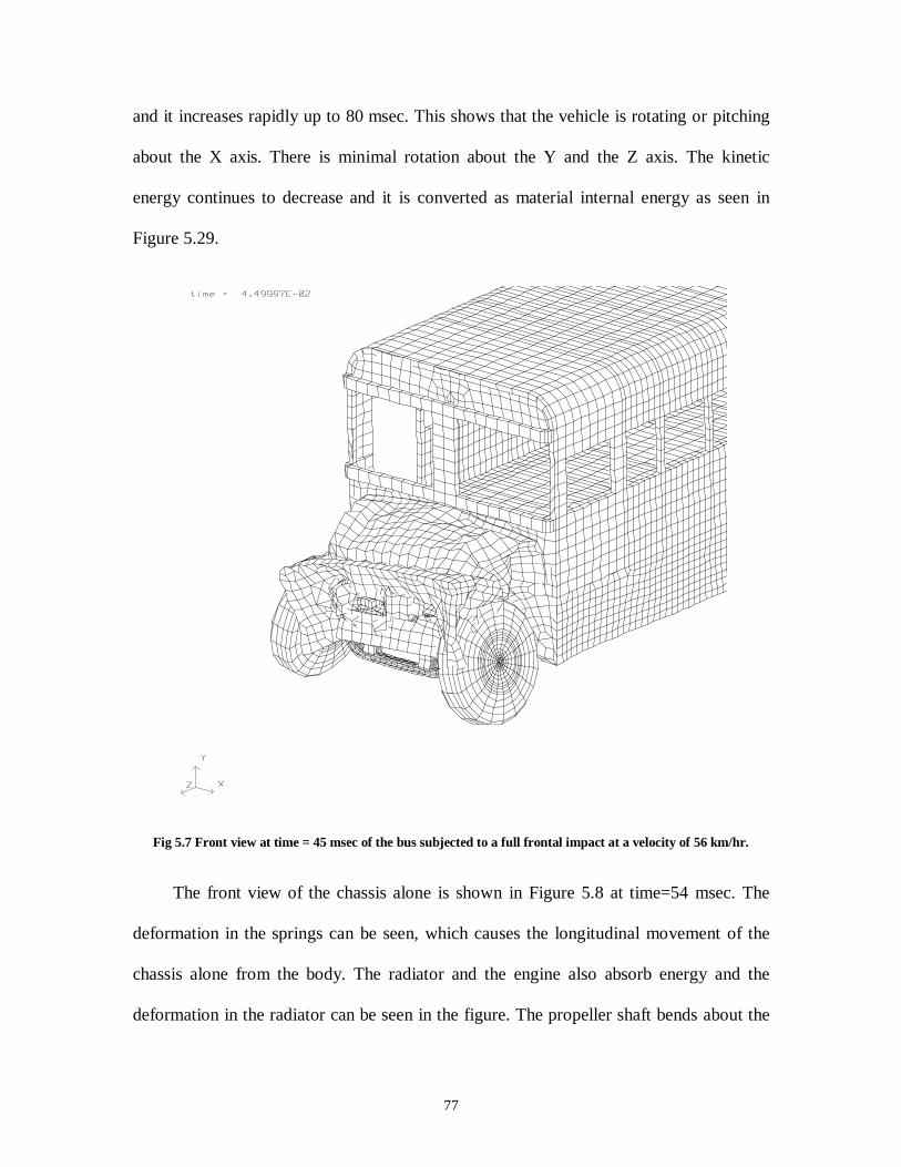
77

and it increases rapidly up to 80 msec. This shows that the vehicle is rotating or pitching

about the X axis. There is minimal rotation about the Y and the Z axis. The kinetic

energy continues to decrease and it is converted as material internal energy as seen in

Figure 5.29.


The front view of the chassis alone is shown in Figure 5.8 at time=54 msec. The

deformation in the springs can be seen, which causes the longitudinal movement of the

chassis alone from the body. The radiator and the engine also absorb energy and the

deformation in the radiator can be seen in the figure. The propeller shaft bends about the

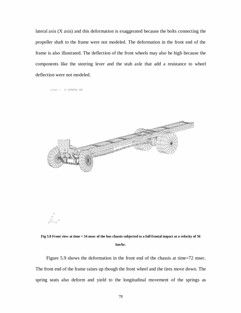
78

lateral axis (X axis) and this deformation is exaggerated because the bolts connecting the

propeller shaft to the frame were not modeled. The deformation in the front end of the

frame is also illustrated. The deflection of the front wheels may also be high because the

components like the steering lever and the stub axle that add a resistance to wheel

deflection were not modeled.

Fig 5.8 Front view at time = 54 msec of the bus chassis subjected to a full frontal impact at a velocity of 56

km/hr.

Figure 5.9 shows the deformation in the front end of the chassis at time=72 msec.

The front end of the frame raises up though the front wheel and the tires move down. The

spring seats also deform and yield to the longitudinal movement of the springs as

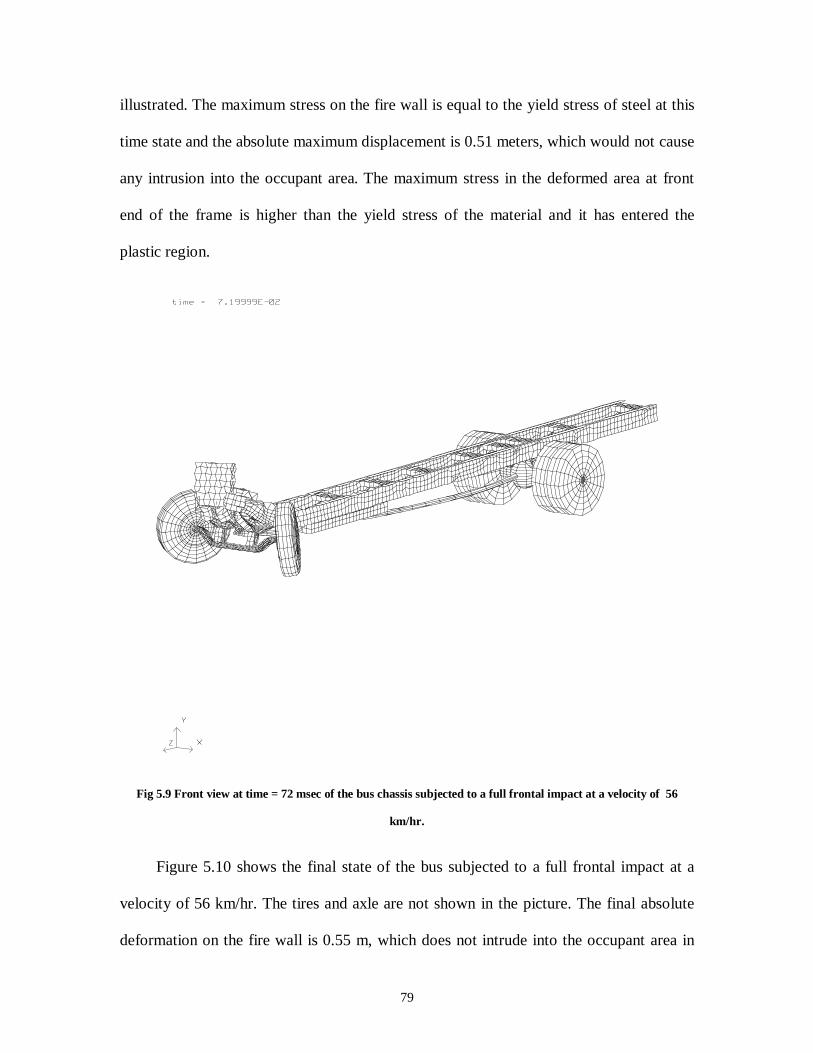
79

illustrated. The maximum stress on the fire wall is equal to the yield stress of steel at this

time state and the absolute maximum displacement is 0.51 meters, which would not cause

any intrusion into the occupant area. The maximum stress in the deformed area at front

end of the frame is higher than the yield stress of the material and it has entered the

plastic region.

Fig 5.9 Front view at time = 72 msec of the bus chassis subjected to a full frontal impact at a velocity of 56

km/hr.

Figure 5.10 shows the final state of the bus subjected to a full frontal impact at a

velocity of 56 km/hr. The tires and axle are not shown in the picture. The final absolute

deformation on the fire wall is 0.55 m, which does not intrude into the occupant area in

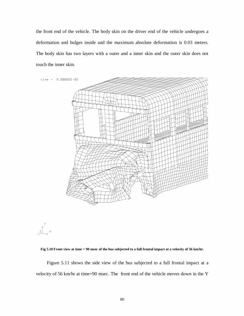
80

the front end of the vehicle. The body skin on the driver end of the vehicle undergoes a

deformation and bulges inside and the maximum absolute deformation is 0.03 meters.

The body skin has two layers with a outer and a inner skin and the outer skin does not

touch the inner skin.


Figure 5.11 shows the side view of the bus subjected to a full frontal impact at a

velocity of 56 km/hr at time=90 msec. The front end of the vehicle moves down in the Y

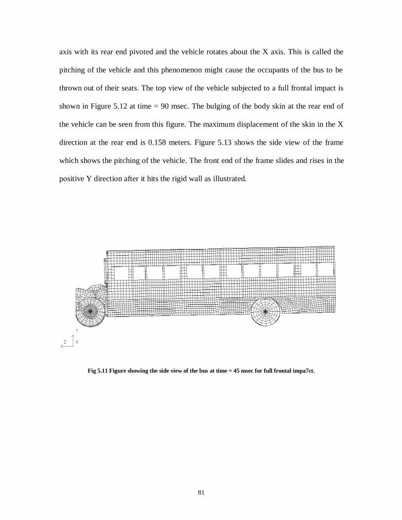
81

axis with its rear end pivoted and the vehicle rotates about the X axis. This is called the

pitching of the vehicle and this phenomenon might cause the occupants of the bus to be

thrown out of their seats. The top view of the vehicle subjected to a full frontal impact is

shown in Figure 5.12 at time = 90 msec. The bulging of the body skin at the rear end of

the vehicle can be seen from this figure. The maximum displacement of the skin in the X

direction at the rear end is 0.158 meters. Figure 5.13 shows the side view of the frame

which shows the pitching of the vehicle. The front end of the frame slides and rises in the

positive Y direction after it hits the rigid wall as illustrated.

Fig 5.11 Figure showing the side view of the bus at time = 45 msec for full frontal impa7ct.

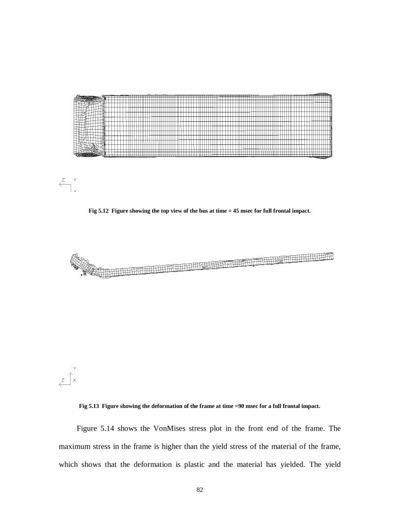
82

Fig 5.12 Figure showing the top view of the bus at time = 45 msec for full frontal impact.

Fig 5.13 Figure showing the deformation of the frame at time =90 msec for a full frontal impact.

Figure 5.14 shows the VonMises stress plot in the front end of the frame. The

maximum stress in the frame is higher than the yield stress of the material of the frame,

which shows that the deformation is plastic and the material has yielded. The yield

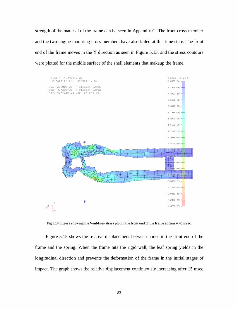
83

strength of the material of the frame can be seen in Appendix C. The front cross member

and the two engine mounting cross members have also failed at this time state. The front

end of the frame moves in the Y direction as seen in Figure 5.13, and the stress contours

were plotted for the middle surface of the shell elements that makeup the frame.

Fig 5.14 Figure showing the VonMises stress plot in the front end of the frame at time = 45 msec.

Figure 5.15 shows the relative displacement between nodes in the front end of the

frame and the spring. When the frame hits the rigid wall, the leaf spring yields in the

longitudinal direction and prevents the deformation of the frame in the initial stages of

impact. The graph shows the relative displacement continuously increasing after 15 msec

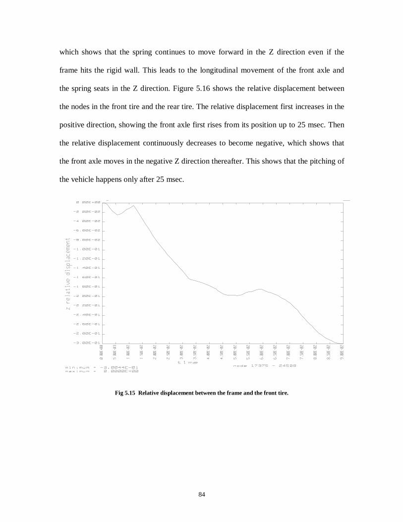
84

which shows that the spring continues to move forward in the Z direction even if the

frame hits the rigid wall. This leads to the longitudinal movement of the front axle and

the spring seats in the Z direction. Figure 5.16 shows the relative displacement between

the nodes in the front tire and the rear tire. The relative displacement first increases in the

positive direction, showing the front axle first rises from its position up to 25 msec. Then

the relative displacement continuously decreases to become negative, which shows that

the front axle moves in the negative Z direction thereafter. This shows that the pitching of

the vehicle happens only after 25 msec.

Fig 5.15 Relative displacement between the frame and the front tire.

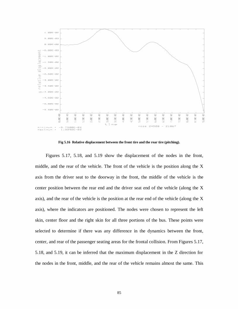
85

Fig 5.16 Relative displacement between the front tire and the rear tire (pitching).

Figures 5.17, 5.18, and 5.19 show the displacement of the nodes in the front,

middle, and the rear of the vehicle. The front of the vehicle is the position along the X

axis from the driver seat to the doorway in the front, the middle of the vehicle is the

center position between the rear end and the driver seat end of the vehicle (along the X

axis), and the rear of the vehicle is the position at the rear end of the vehicle (along the X

axis), where the indicators are positioned. The nodes were chosen to represent the left

skin, center floor and the right skin for all three portions of the bus. These points were

selected to determine if there was any difference in the dynamics between the front,

center, and rear of the passenger seating areas for the frontal collision. From Figures 5.17,

5.18, and 5.19, it can be inferred that the maximum displacement in the Z direction for

the nodes in the front, middle, and the rear of the vehicle remains almost the same. This

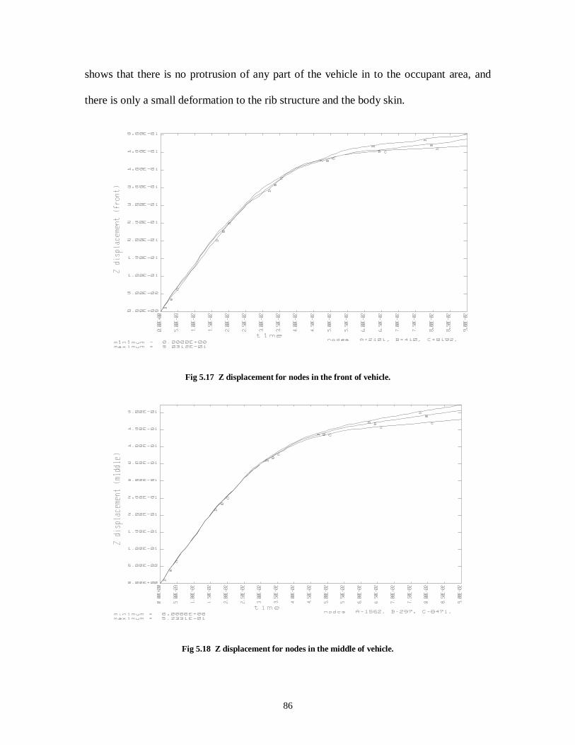
86

shows that there is no protrusion of any part of the vehicle in to the occupant area, and

there is only a small deformation to the rib structure and the body skin.

Fig 5.17 Z displacement for nodes in the front of vehicle.

Fig 5.18 Z displacement for nodes in the middle of vehicle.

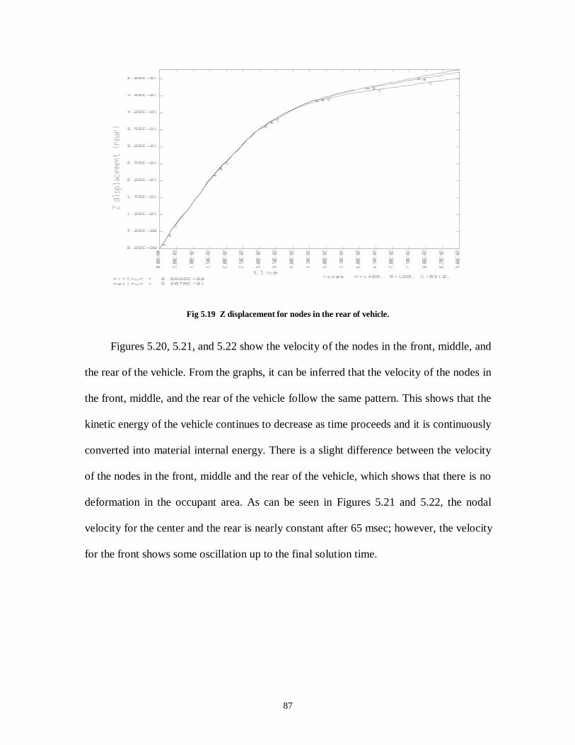
87

Fig 5.19 Z displacement for nodes in the rear of vehicle.

Figures 5.20, 5.21, and 5.22 show the velocity of the nodes in the front, middle, and

the rear of the vehicle. From the graphs, it can be inferred that the velocity of the nodes in

the front, middle, and the rear of the vehicle follow the same pattern. This shows that the

kinetic energy of the vehicle continues to decrease as time proceeds and it is continuously

converted into material internal energy. There is a slight difference between the velocity

of the nodes in the front, middle and the rear of the vehicle, which shows that there is no

deformation in the occupant area. As can be seen in Figures 5.21 and 5.22, the nodal

velocity for the center and the rear is nearly constant after 65 msec; however, the velocity

for the front shows some oscillation up to the final solution time.

88

Fig 5.20 Z velocity for nodes in the front of vehicle.

Fig 5.21 Z velocity for nodes in the middle of vehicle.

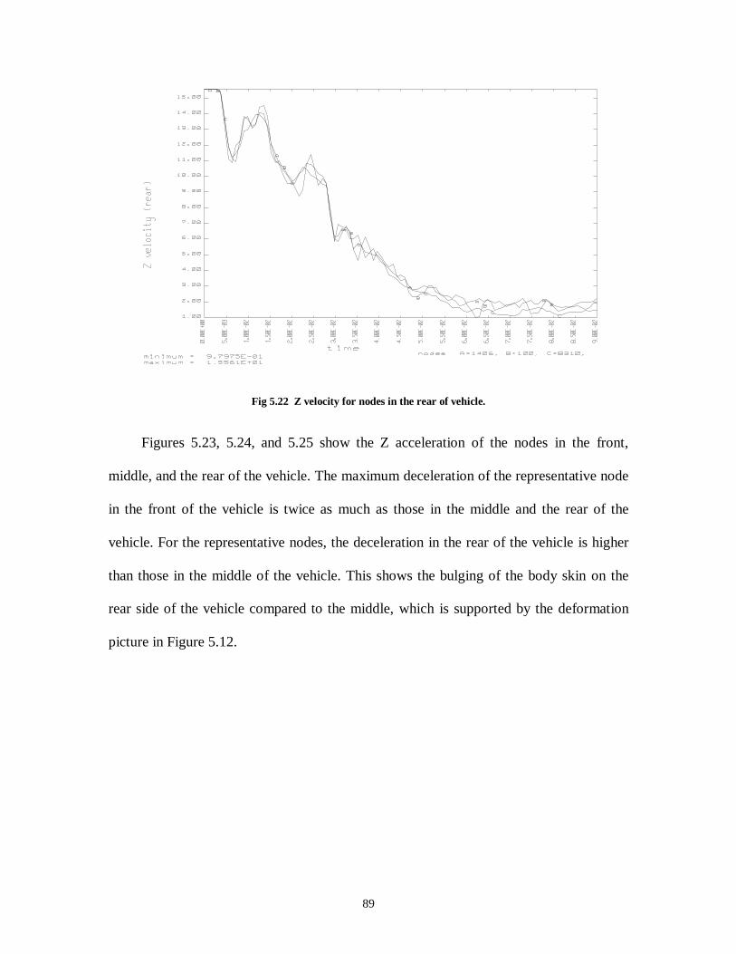
89

Fig 5.22 Z velocity for nodes in the rear of vehicle.

Figures 5.23, 5.24, and 5.25 show the Z acceleration of the nodes in the front,

middle, and the rear of the vehicle. The maximum deceleration of the representative node

in the front of the vehicle is twice as much as those in the middle and the rear of the

vehicle. For the representative nodes, the deceleration in the rear of the vehicle is higher

than those in the middle of the vehicle. This shows the bulging of the body skin on the

rear side of the vehicle compared to the middle, which is supported by the deformation

picture in Figure 5.12.

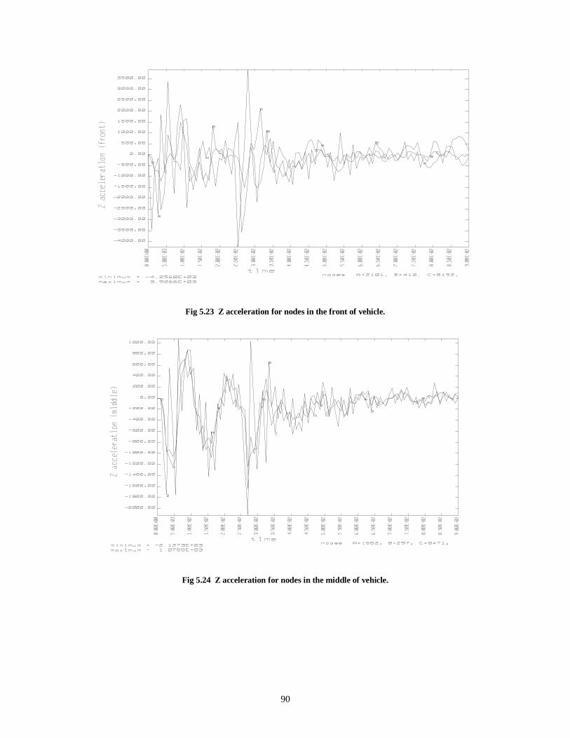
90

Fig 5.23 Z acceleration for nodes in the front of vehicle.

Fig 5.24 Z acceleration for nodes in the middle of vehicle.

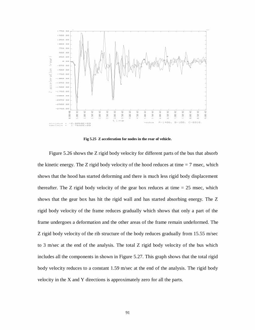
91

Fig 5.25 Z acceleration for nodes in the rear of vehicle.

Figure 5.26 shows the Z rigid body velocity for different parts of the bus that absorb

the kinetic energy. The Z rigid body velocity of the hood reduces at time = 7 msec, which

shows that the hood has started deforming and there is much less rigid body displacement

thereafter. The Z rigid body velocity of the gear box reduces at time = 25 msec, which

shows that the gear box has hit the rigid wall and has started absorbing energy. The Z

rigid body velocity of the frame reduces gradually which shows that only a part of the

frame undergoes a deformation and the other areas of the frame remain undeformed. The

Z rigid body velocity of the rib structure of the body reduces gradually from 15.55 m/sec

to 3 m/sec at the end of the analysis. The total Z rigid body velocity of the bus which

includes all the components in shown in Figure 5.27. This graph shows that the total rigid

body velocity reduces to a constant 1.59 m/sec at the end of the analysis. The rigid body

velocity in the X and Y directions is approximately zero for all the parts.

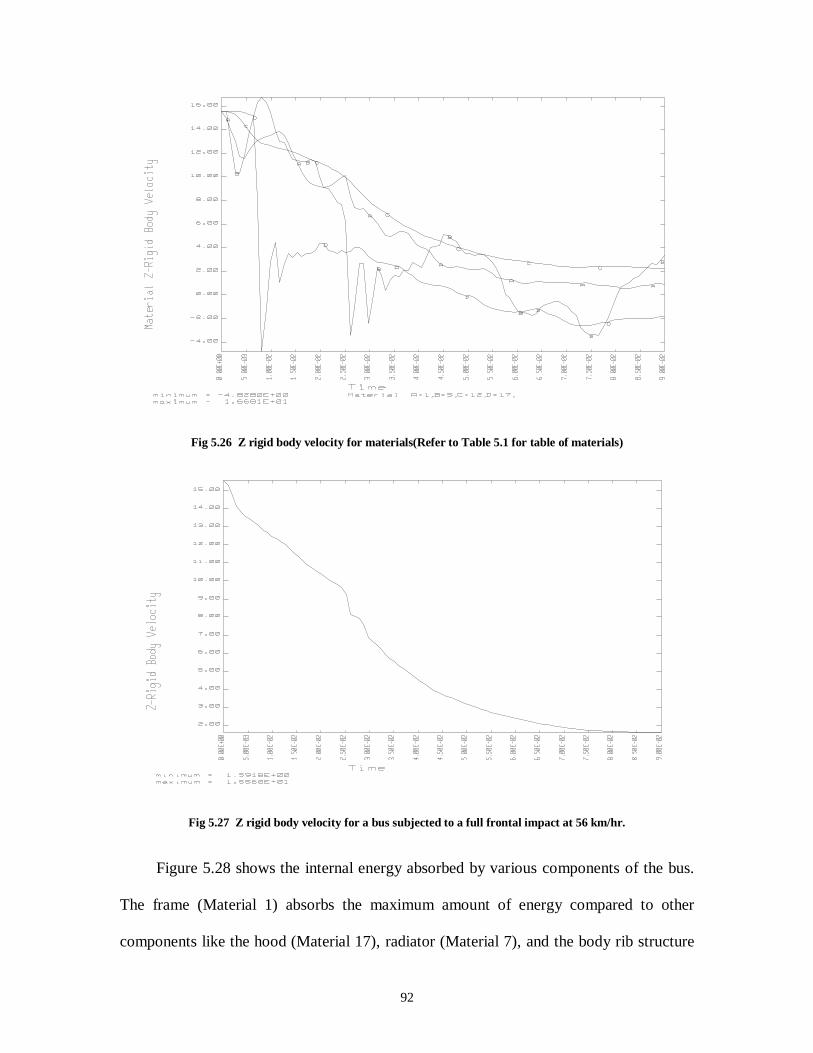
92

Fig 5.26 Z rigid body velocity for materials(Refer to Table 5.1 for table of materials)

Fig 5.27 Z rigid body velocity for a bus subjected to a full frontal impact at 56 km/hr.

Figure 5.28 shows the internal energy absorbed by various components of the bus.

The frame (Material 1) absorbs the maximum amount of energy compared to other

components like the hood (Material 17), radiator (Material 7), and the body rib structure

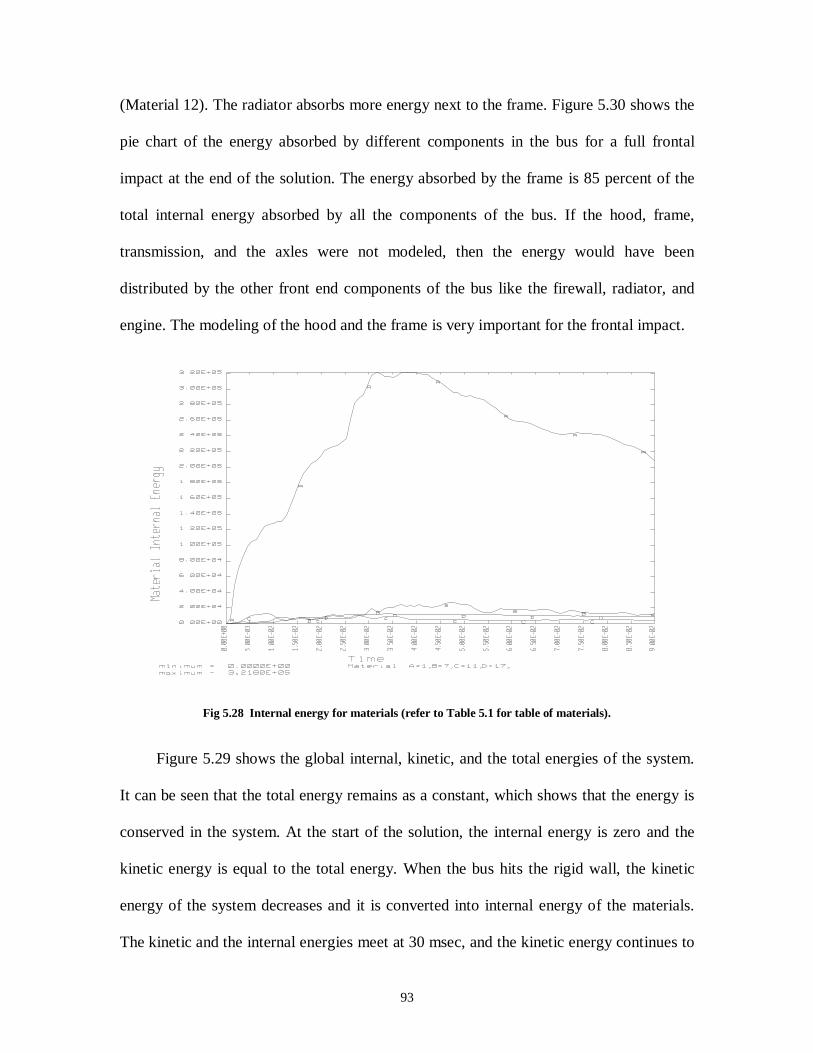
93

(Material 12). The radiator absorbs more energy next to the frame. Figure 5.30 shows the

pie chart of the energy absorbed by different components in the bus for a full frontal

impact at the end of the solution. The energy absorbed by the frame is 85 percent of the

total internal energy absorbed by all the components of the bus. If the hood, frame,

transmission, and the axles were not modeled, then the energy would have been

distributed by the other front end components of the bus like the firewall, radiator, and

engine. The modeling of the hood and the frame is very important for the frontal impact.

Fig 5.28 Internal energy for materials (refer to Table 5.1 for table of materials).

Figure 5.29 shows the global internal, kinetic, and the total energies of the system.

It can be seen that the total energy remains as a constant, which shows that the energy is

conserved in the system. At the start of the solution, the internal energy is zero and the

kinetic energy is equal to the total energy. When the bus hits the rigid wall, the kinetic

energy of the system decreases and it is converted into internal energy of the materials.

The kinetic and the internal energies meet at 30 msec, and the kinetic energy continues to

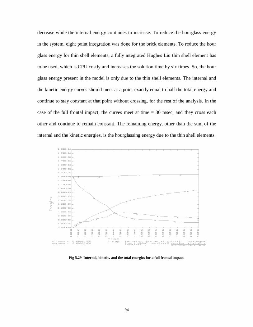
94

decrease while the internal energy continues to increase. To reduce the hourglass energy

in the system, eight point integration was done for the brick elements. To reduce the hour

glass energy for thin shell elements, a fully integrated Hughes Liu thin shell element has

to be used, which is CPU costly and increases the solution time by six times. So, the hour

glass energy present in the model is only due to the thin shell elements. The internal and

the kinetic energy curves should meet at a point exactly equal to half the total energy and

continue to stay constant at that point without crossing, for the rest of the analysis. In the

case of the full frontal impact, the curves meet at time = 30 msec, and they cross each

other and continue to remain constant. The remaining energy, other than the sum of the

internal and the kinetic energies, is the hourglassing energy due to the thin shell elements.

Fig 5.29 Internal, kinetic, and the total energies for a full frontal impact.

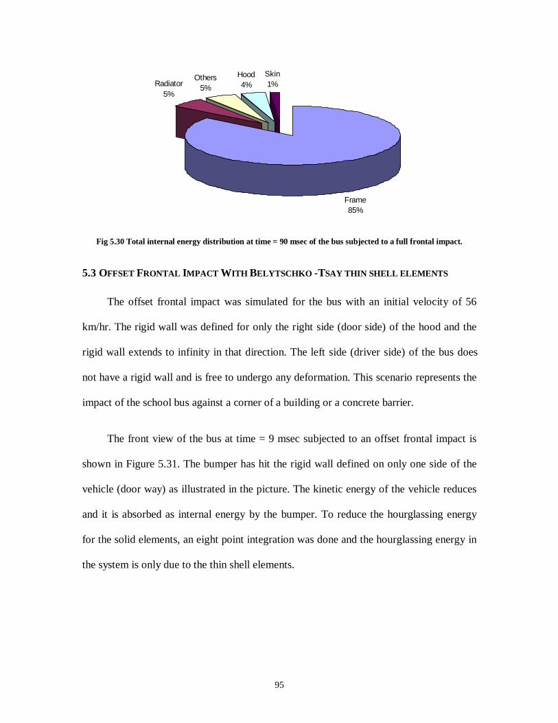
95

Frame85%

Radiator5%

Others5%

Hood4%

Skin1%

Fig 5.30 Total internal energy distribution at time = 90 msec of the bus subjected to a full frontal impact.

5.3 OFFSET FRONTAL IMPACT WITH BELYTSCHKO -TSAY THIN SHELL ELEMENTS

The offset frontal impact was simulated for the bus with an initial velocity of 56

km/hr. The rigid wall was defined for only the right side (door side) of the hood and the

rigid wall extends to infinity in that direction. The left side (driver side) of the bus does

not have a rigid wall and is free to undergo any deformation. This scenario represents the

impact of the school bus against a corner of a building or a concrete barrier.

The front view of the bus at time = 9 msec subjected to an offset frontal impact is

shown in Figure 5.31. The bumper has hit the rigid wall defined on only one side of the

vehicle (door way) as illustrated in the picture. The kinetic energy of the vehicle reduces

and it is absorbed as internal energy by the bumper. To reduce the hourglassing energy

for the solid elements, an eight point integration was done and the hourglassing energy in

the system is only due to the thin shell elements.

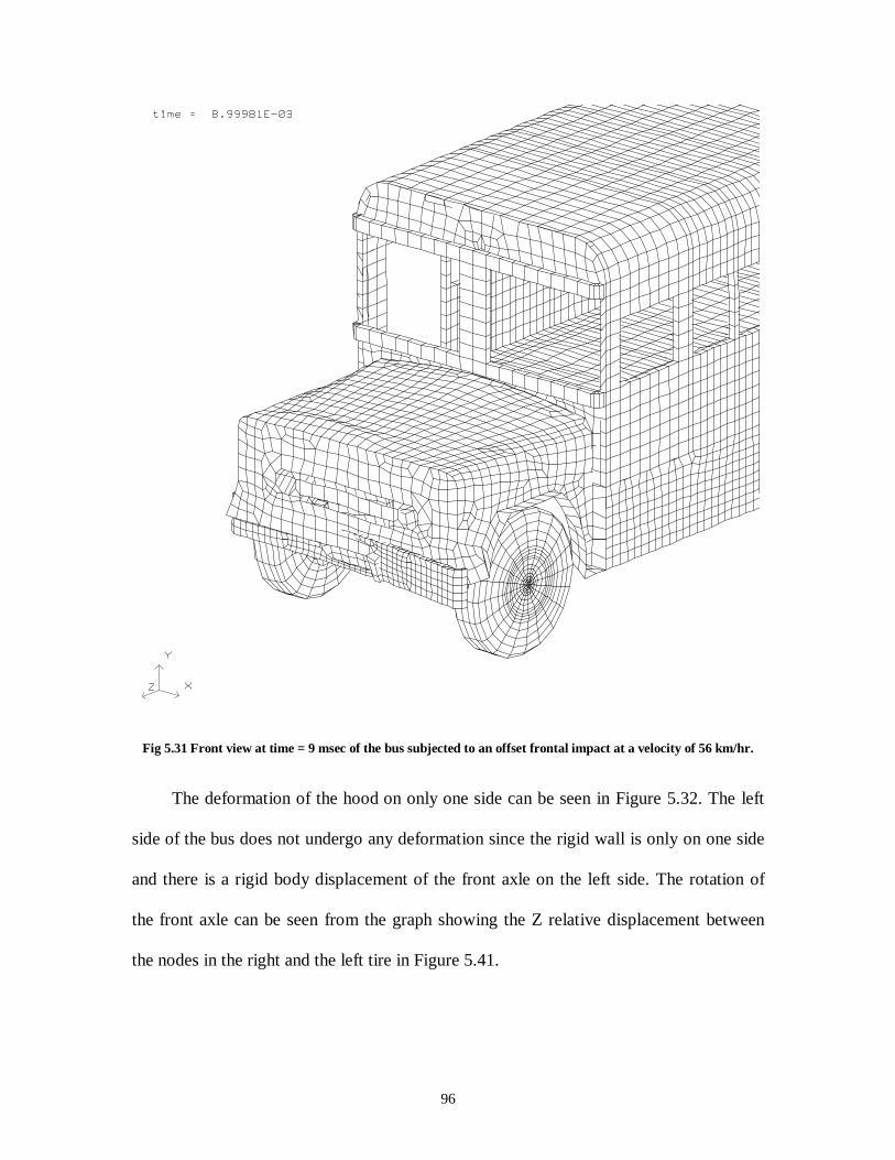
96

Fig 5.31 Front view at time = 9 msec of the bus subjected to an offset frontal impact at a velocity of 56 km/hr.

The deformation of the hood on only one side can be seen in Figure 5.32. The left

side of the bus does not undergo any deformation since the rigid wall is only on one side

and there is a rigid body displacement of the front axle on the left side. The rotation of

the front axle can be seen from the graph showing the Z relative displacement between

the nodes in the right and the left tire in Figure 5.41.

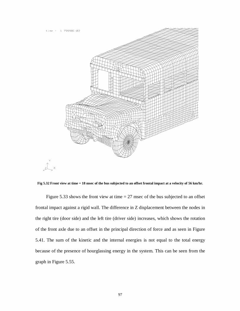
97


Figure 5.33 shows the front view at time = 27 msec of the bus subjected to an offset

frontal impact against a rigid wall. The difference in Z displacement between the nodes in

the right tire (door side) and the left tire (driver side) increases, which shows the rotation

of the front axle due to an offset in the principal direction of force and as seen in Figure

5.41. The sum of the kinetic and the internal energies is not equal to the total energy

because of the presence of hourglassing energy in the system. This can be seen from the

graph in Figure 5.55.

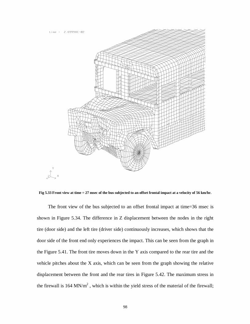
98


The front view of the bus subjected to an offset frontal impact at time=36 msec is

shown in Figure 5.34. The difference in Z displacement between the nodes in the right

tire (door side) and the left tire (driver side) continuously increases, which shows that the

door side of the front end only experiences the impact. This can be seen from the graph in

the Figure 5.41. The front tire moves down in the Y axis compared to the rear tire and the

vehicle pitches about the X axis, which can be seen from the graph showing the relative

displacement between the front and the rear tires in Figure 5.42. The maximum stress in

the firewall is 164 MN/m2 , which is within the yield stress of the material of the firewall;

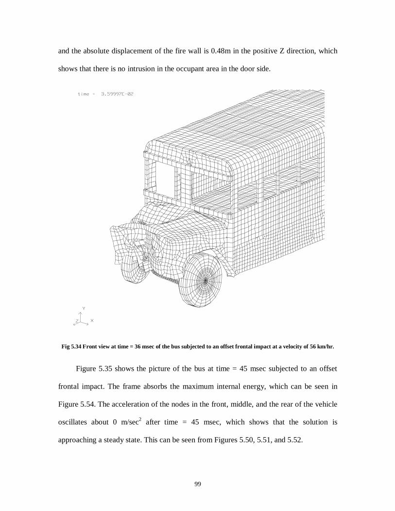
99

and the absolute displacement of the fire wall is 0.48m in the positive Z direction, which

shows that there is no intrusion in the occupant area in the door side.


Figure 5.35 shows the picture of the bus at time = 45 msec subjected to an offset

frontal impact. The frame absorbs the maximum internal energy, which can be seen in

Figure 5.54. The acceleration of the nodes in the front, middle, and the rear of the vehicle

oscillates about 0 m/sec2 after time = 45 msec, which shows that the solution is

approaching a steady state. This can be seen from Figures 5.50, 5.51, and 5.52.

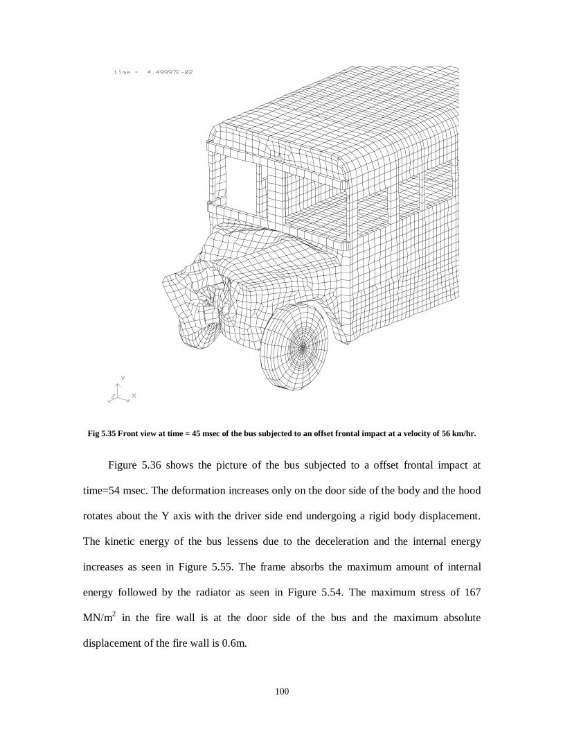
100


Figure 5.36 shows the picture of the bus subjected to a offset frontal impact at

time=54 msec. The deformation increases only on the door side of the body and the hood

rotates about the Y axis with the driver side end undergoing a rigid body displacement.

The kinetic energy of the bus lessens due to the deceleration and the internal energy

increases as seen in Figure 5.55. The frame absorbs the maximum amount of internal

energy followed by the radiator as seen in Figure 5.54. The maximum stress of 167

MN/m2 in the fire wall is at the door side of the bus and the maximum absolute

displacement of the fire wall is 0.6m.

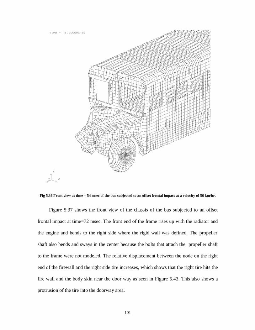
101


Figure 5.37 shows the front view of the chassis of the bus subjected to an offset

frontal impact at time=72 msec. The front end of the frame rises up with the radiator and

the engine and bends to the right side where the rigid wall was defined. The propeller

shaft also bends and sways in the center because the bolts that attach the propeller shaft

to the frame were not modeled. The relative displacement between the node on the right

end of the firewall and the right side tire increases, which shows that the right tire hits the

fire wall and the body skin near the door way as seen in Figure 5.43. This also shows a

protrusion of the tire into the doorway area.

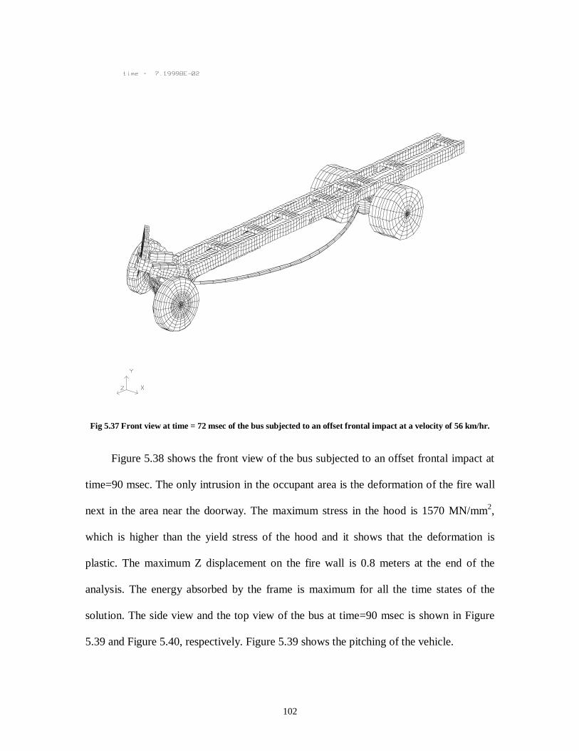
102


Figure 5.38 shows the front view of the bus subjected to an offset frontal impact at

time=90 msec. The only intrusion in the occupant area is the deformation of the fire wall

next in the area near the doorway. The maximum stress in the hood is 1570 MN/mm2,

which is higher than the yield stress of the hood and it shows that the deformation is

plastic. The maximum Z displacement on the fire wall is 0.8 meters at the end of the

analysis. The energy absorbed by the frame is maximum for all the time states of the

solution. The side view and the top view of the bus at time=90 msec is shown in Figure

5.39 and Figure 5.40, respectively. Figure 5.39 shows the pitching of the vehicle.

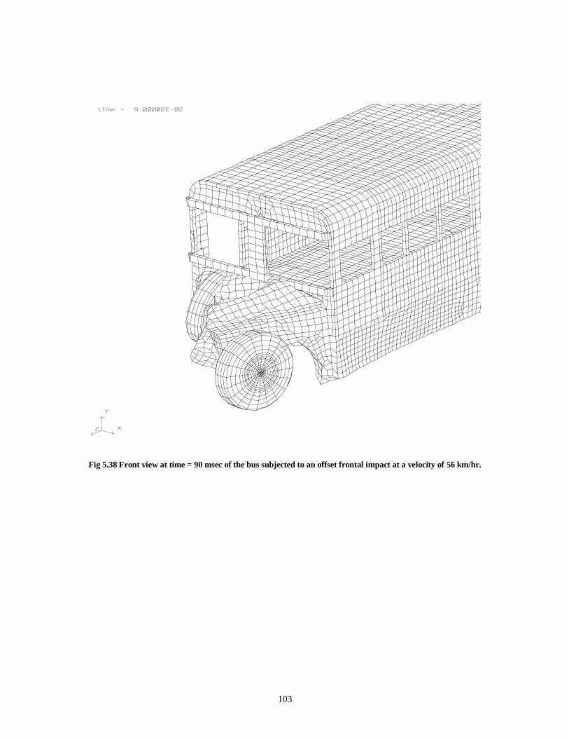
103


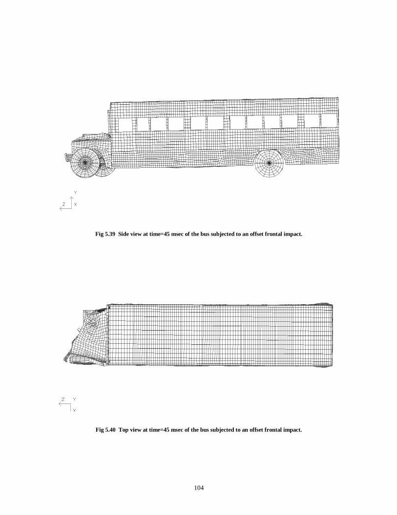
104

Fig 5.39 Side view at time=45 msec of the bus subjected to an offset frontal impact.

Fig 5.40 Top view at time=45 msec of the bus subjected to an offset frontal impact.

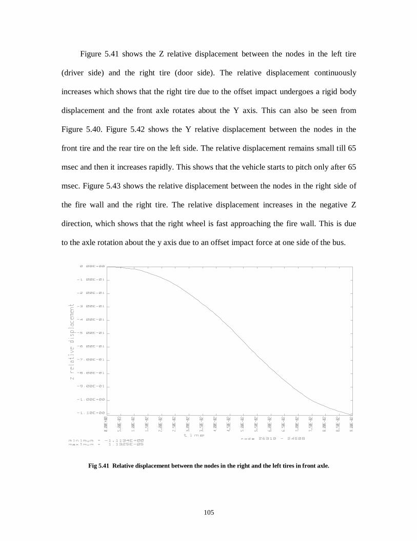
105

Figure 5.41 shows the Z relative displacement between the nodes in the left tire

(driver side) and the right tire (door side). The relative displacement continuously

increases which shows that the right tire due to the offset impact undergoes a rigid body

displacement and the front axle rotates about the Y axis. This can also be seen from

Figure 5.40. Figure 5.42 shows the Y relative displacement between the nodes in the

front tire and the rear tire on the left side. The relative displacement remains small till 65

msec and then it increases rapidly. This shows that the vehicle starts to pitch only after 65

msec. Figure 5.43 shows the relative displacement between the nodes in the right side of

the fire wall and the right tire. The relative displacement increases in the negative Z

direction, which shows that the right wheel is fast approaching the fire wall. This is due

to the axle rotation about the y axis due to an offset impact force at one side of the bus.

Fig 5.41 Relative displacement between the nodes in the right and the left tires in front axle.

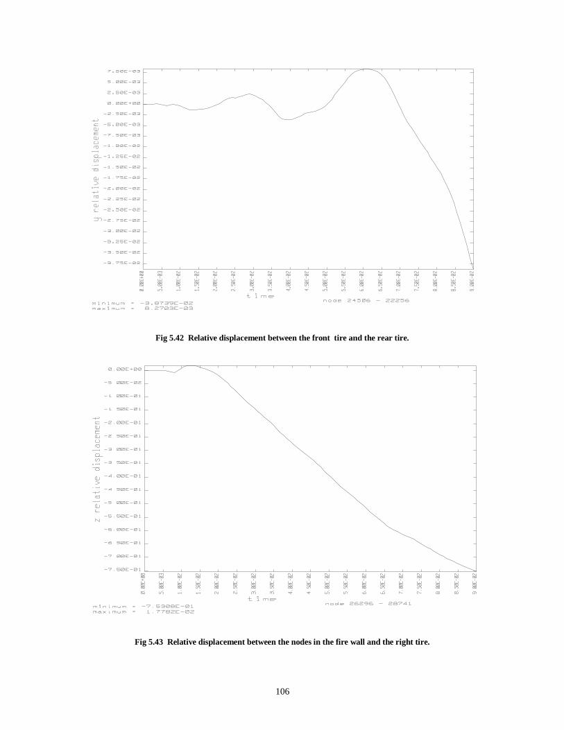
106

Fig 5.42 Relative displacement between the front tire and the rear tire.

Fig 5.43 Relative displacement between the nodes in the fire wall and the right tire.

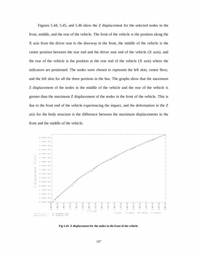
107

Figures 5.44, 5.45, and 5.46 show the Z displacement for the selected nodes in the

front, middle, and the rear of the vehicle. The front of the vehicle is the position along the

X axis from the driver seat to the doorway in the front, the middle of the vehicle is the

center position between the rear end and the driver seat end of the vehicle (X axis), and

the rear of the vehicle is the position at the rear end of the vehicle (X axis) where the

indicators are positioned. The nodes were chosen to represent the left skin, center floor,

and the left skin for all the three portions in the bus. The graphs show that the maximum

Z displacement of the nodes in the middle of the vehicle and the rear of the vehicle is

greater than the maximum Z displacement of the nodes in the front of the vehicle. This is

due to the front end of the vehicle experiencing the impact, and the deformation in the Z

axis for the body structure is the difference between the maximum displacements in the

front and the middle of the vehicle.

Fig 5.44 Z displacement for the nodes in the front of the vehicle.

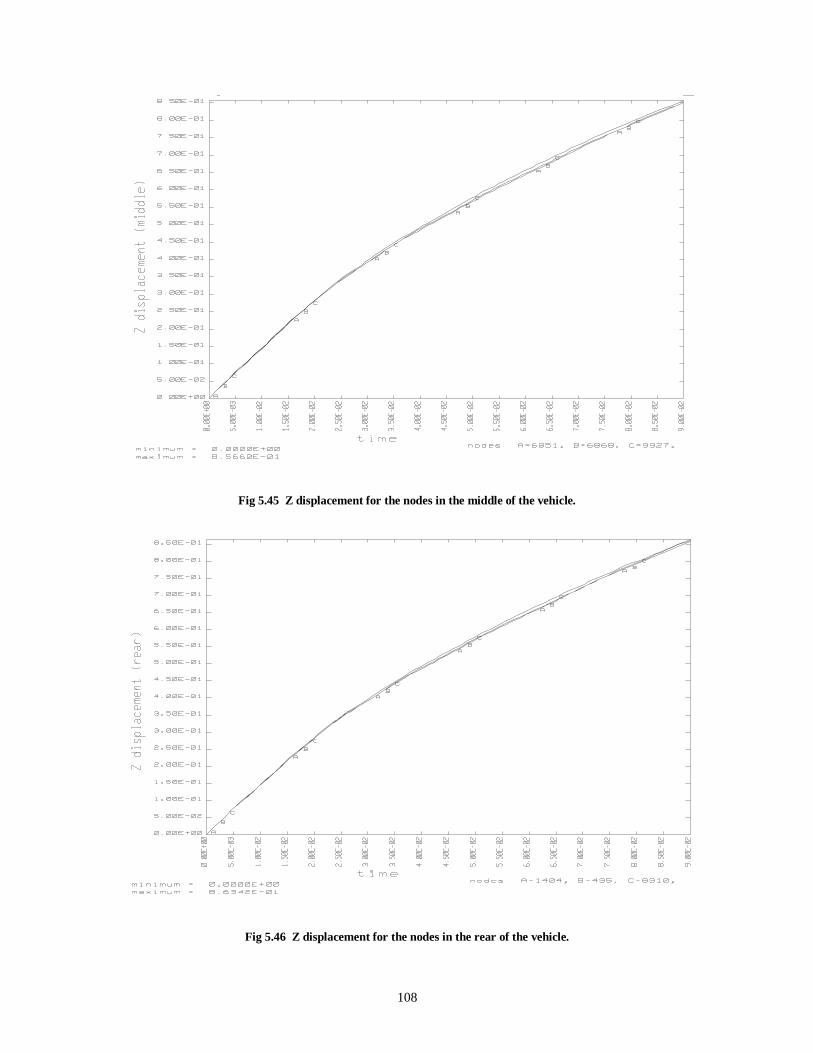
108

Fig 5.45 Z displacement for the nodes in the middle of the vehicle.

Fig 5.46 Z displacement for the nodes in the rear of the vehicle.

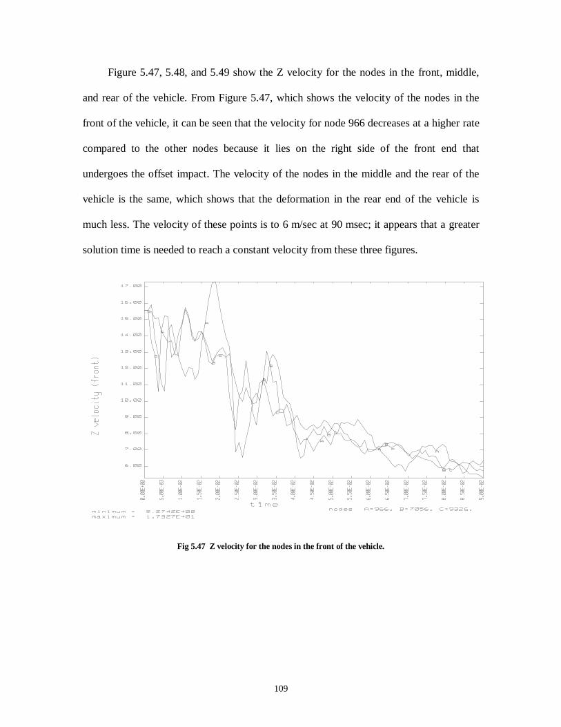
109

Figure 5.47, 5.48, and 5.49 show the Z velocity for the nodes in the front, middle,

and rear of the vehicle. From Figure 5.47, which shows the velocity of the nodes in the

front of the vehicle, it can be seen that the velocity for node 966 decreases at a higher rate

compared to the other nodes because it lies on the right side of the front end that

undergoes the offset impact. The velocity of the nodes in the middle and the rear of the

vehicle is the same, which shows that the deformation in the rear end of the vehicle is

much less. The velocity of these points is to 6 m/sec at 90 msec; it appears that a greater

solution time is needed to reach a constant velocity from these three figures.

Fig 5.47 Z velocity for the nodes in the front of the vehicle.

110

Fig 5.48 Z velocity for the nodes in the middle of the vehicle.

Fig 5.49 Z velocity for the nodes in the rear of the vehicle.

111

Figure 5.50, 5.51, and 5.52 show the Z acceleration for the nodes in the front,

middle, and rear of the vehicle. From Figure 5.50, it can be seen that the maximum

deceleration for node 966 is higher than the other nodes in the front of the vehicle. This is

because node 966 lies on the right end of the front of the vehicle near the doorway that

experiences the offset impact. From Figure 5.51, it can be seen that the maximum

deceleration of node 6851 is higher than the other nodes. This is because this node lies on

the right end of the vehicle at the middle, where the front of the vehicle on the same side

undergoes an impact. This rapid deceleration causes a bulging of the body structure, and

the skin on the right side and this phenomenon is supported by the top view of the vehicle

in Figure 5.40. The Z deceleration of the nodes in the rear of the vehicle is small

compared to the front and the middle portion of the vehicle. However, due to this

deceleration, the rear body skin undergoes a bulging that can be seen from the top view

of the vehicle in Figure 5.40. The acceleration of the nodes in the three figures appear to

be oscillating about 0 m/sec2; thus the bus is approaching steady state.

112

Fig 5.50 Z acceleration for nodes in the front of the vehicle.

Fig 5.51 Z acceleration for the nodes in the middle of the vehicle.

113

Fig 5.52 Z acceleration of the nodes in the rear of the vehicle.

Figure 5.50 shows the Z rigid body velocity for different components of the bus.

The rigid body velocity of the radiator decreases rapidly at time = 5 msec which shows

that the radiator has started deforming and the rigid body velocity reduces to zero at this

time. The rigid body velocity for the hood decreases gradually and becomes zero only at

the end of the analysis. The rigid body velocity for the frame lessens gradually, which

shows that the final shape of the frame is a combination of the deformation and a rigid

body velocity in which the frame slides and rises up against the rigid wall. This can be

seen from Figure 5.34.

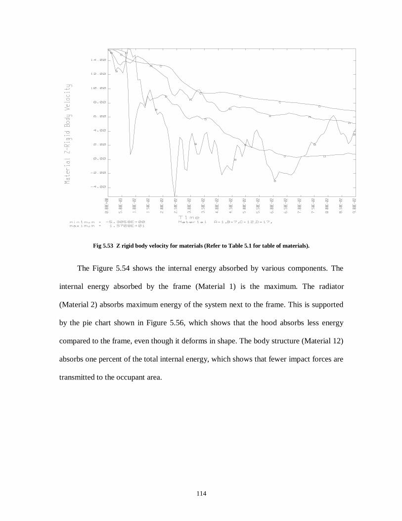
114

Fig 5.53 Z rigid body velocity for materials (Refer to Table 5.1 for table of materials).

The Figure 5.54 shows the internal energy absorbed by various components. The

internal energy absorbed by the frame (Material 1) is the maximum. The radiator

(Material 2) absorbs maximum energy of the system next to the frame. This is supported

by the pie chart shown in Figure 5.56, which shows that the hood absorbs less energy

compared to the frame, even though it deforms in shape. The body structure (Material 12)

absorbs one percent of the total internal energy, which shows that fewer impact forces are

transmitted to the occupant area.

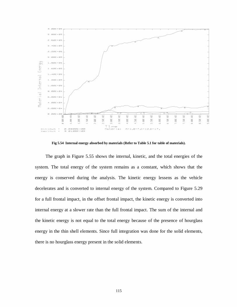
115

Fig 5.54 Internal energy absorbed by materials (Refer to Table 5.1 for table of materials).

The graph in Figure 5.55 shows the internal, kinetic, and the total energies of the

system. The total energy of the system remains as a constant, which shows that the

energy is conserved during the analysis. The kinetic energy lessens as the vehicle

decelerates and is converted to internal energy of the system. Compared to Figure 5.29

for a full frontal impact, in the offset frontal impact, the kinetic energy is converted into

internal energy at a slower rate than the full frontal impact. The sum of the internal and

the kinetic energy is not equal to the total energy because of the presence of hourglass

energy in the thin shell elements. Since full integration was done for the solid elements,

there is no hourglass energy present in the solid elements.

116

Fig 5.55 Kinetic, internal and the total energies for an offset frontal impact.

Frame85%

Radiator8%

Others3%

Hood3%

Ribs1%

Fig 5.56 Total internal energy distribution at time = 90 msec of the bus subjected to an offset frontal impact.

5.4 HIGHER ORDER INTEGRATION FOR THIN SHELL ELEMENTS

The hourglassing energy for the thin shell elements was high for the analysis run

before and it was equal to the magnitude of the kinetic energy. To avoid the hourglass

energy for the thin shell elements, Hughes-Liu elements with Selective-Reduced

117

integration have to be used. Since these elements are integrated using 2 X 2 Gaussian

quadrature in the plane, these elements are recommended in areas where zero energy

modes (hour glassing) is a problem. Using these elements, the run time for the analysis is

increased by five times the previous analyse’s. So the analysis was terminated as soon as

the solution reached a steady state, (i.e.) when the velocity became constant or the

acceleration became zero. A comparison is made between the analyses with and without

hour glassing for a full frontal impact to find the differences in the energy management,

deformation, displacement, velocity, and acceleration.

The Hughes-Liu elements with selective reduced (SR) integration were used for all

the thin shell elements in the model. No changes were made in the mesh density and the

total number of elements in each part remained the same. The initial and the boundary

conditions remained the same for the analyses. The hourglassing energy remained zero

through out the analysis because eight-point integration was done for the solid elements

and Hughes-Liu element formulation was used for the thin shell elements. The total

energy remained as a constant, which was equal to the sum of the kinetic and the internal

energies at all time states.

5.5 FULL FRONTAL IMPACT WITH HUGHES-LIU SR THIN SHELL ELEMENTS

Figure 5.57 shows the front view of the vehicle at time = 0 msec. The initial

conditions and the boundary conditions were the same for both analyses run with the

single point integration and the Hughes-Liu SR thin shell elements. The only difference

between the two analyses is the element formulation for the thin shell elements.

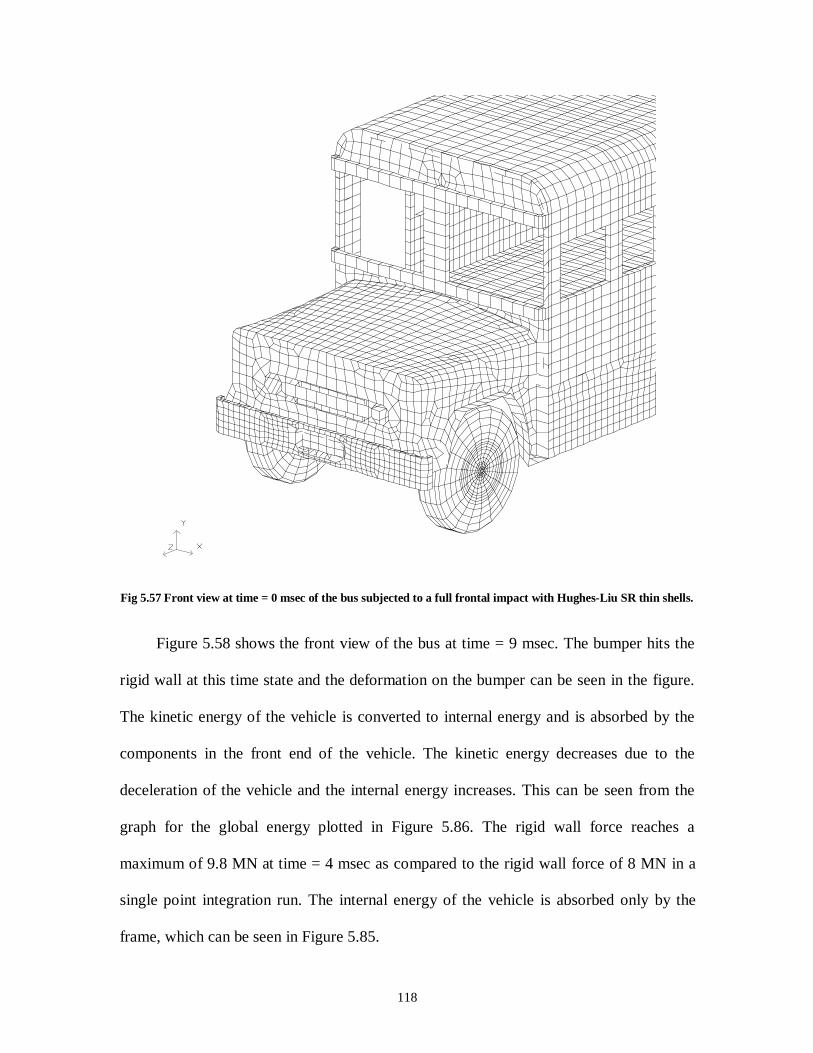
118

Fig 5.57 Front view at time = 0 msec of the bus subjected to a full frontal impact with Hughes-Liu SR thin shells.

Figure 5.58 shows the front view of the bus at time = 9 msec. The bumper hits the

rigid wall at this time state and the deformation on the bumper can be seen in the figure.

The kinetic energy of the vehicle is converted to internal energy and is absorbed by the

components in the front end of the vehicle. The kinetic energy decreases due to the

deceleration of the vehicle and the internal energy increases. This can be seen from the

graph for the global energy plotted in Figure 5.86. The rigid wall force reaches a

maximum of 9.8 MN at time = 4 msec as compared to the rigid wall force of 8 MN in a

single point integration run. The internal energy of the vehicle is absorbed only by the

frame, which can be seen in Figure 5.85.

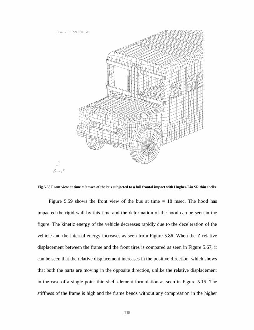
119

Fig 5.58 Front view at time = 9 msec of the bus subjected to a full frontal impact with Hughes-Liu SR thin shells.

Figure 5.59 shows the front view of the bus at time = 18 msec. The hood has

impacted the rigid wall by this time and the deformation of the hood can be seen in the

figure. The kinetic energy of the vehicle decreases rapidly due to the deceleration of the

vehicle and the internal energy increases as seen from Figure 5.86. When the Z relative

displacement between the frame and the front tires is compared as seen in Figure 5.67, it

can be seen that the relative displacement increases in the positive direction, which shows

that both the parts are moving in the opposite direction, unlike the relative displacement

in the case of a single point thin shell element formulation as seen in Figure 5.15. The

stiffness of the frame is high and the frame bends without any compression in the higher

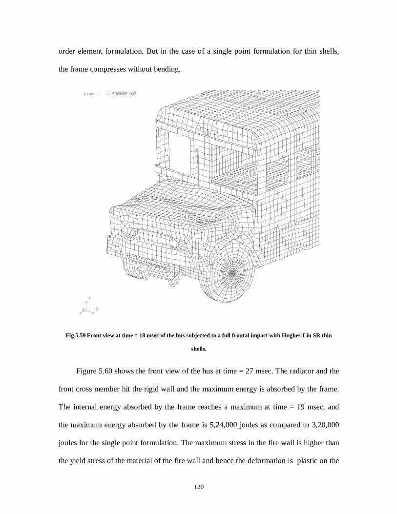
120

order element formulation. But in the case of a single point formulation for thin shells,

the frame compresses without bending.

Fig 5.59 Front view at time = 18 msec of the bus subjected to a full frontal impact with Hughes-Liu SR thin

shells.

Figure 5.60 shows the front view of the bus at time = 27 msec. The radiator and the

front cross member hit the rigid wall and the maximum energy is absorbed by the frame.

The internal energy absorbed by the frame reaches a maximum at time = 19 msec, and

the maximum energy absorbed by the frame is 5,24,000 joules as compared to 3,20,000

joules for the single point formulation. The maximum stress in the fire wall is higher than

the yield stress of the material of the fire wall and hence the deformation is plastic on the

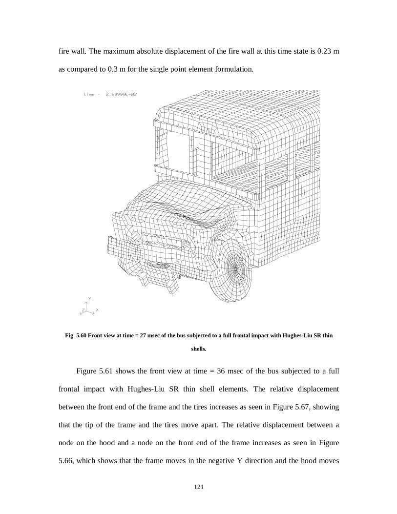
121

fire wall. The maximum absolute displacement of the fire wall at this time state is 0.23 m

as compared to 0.3 m for the single point element formulation.


shells.

Figure 5.61 shows the front view at time = 36 msec of the bus subjected to a full

frontal impact with Hughes-Liu SR thin shell elements. The relative displacement

between the front end of the frame and the tires increases as seen in Figure 5.67, showing

that the tip of the frame and the tires move apart. The relative displacement between a

node on the hood and a node on the front end of the frame increases as seen in Figure

5.66, which shows that the frame moves in the negative Y direction and the hood moves

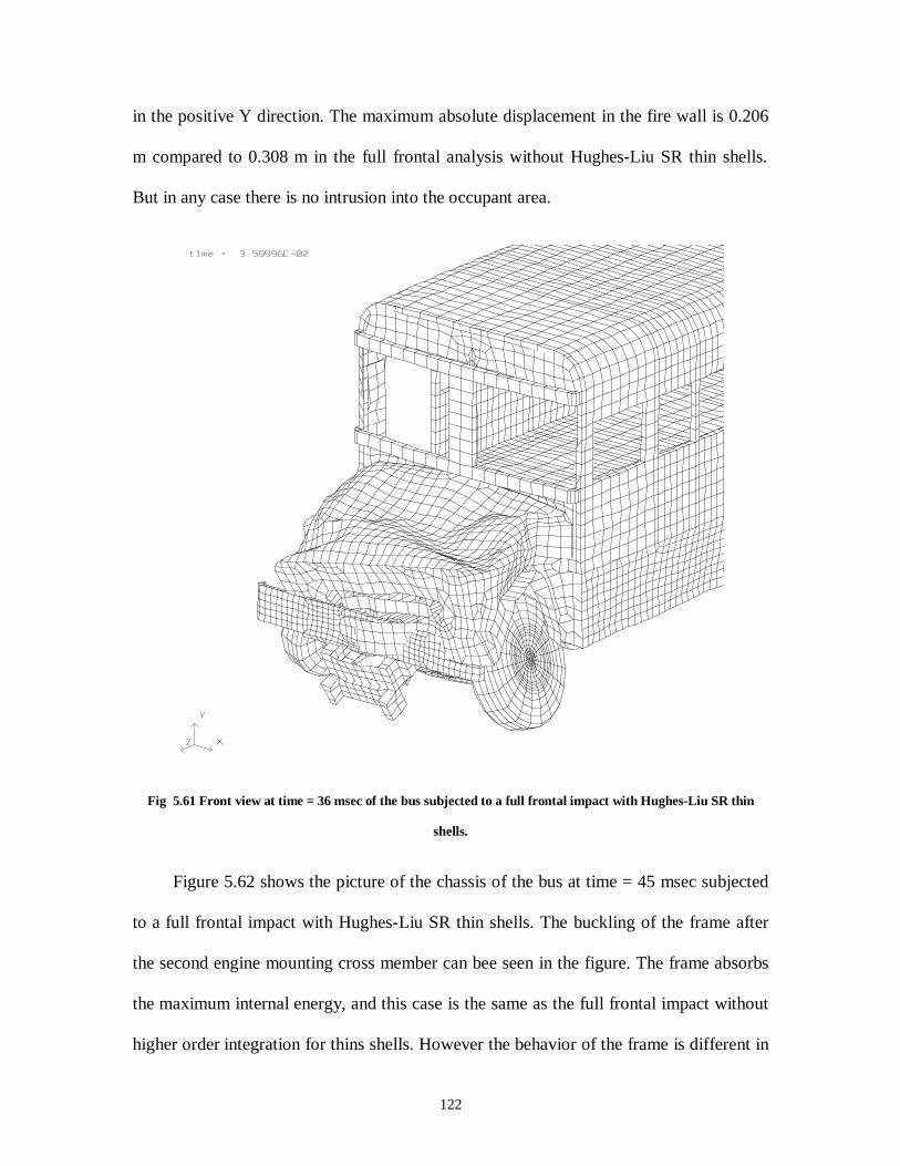
122

in the positive Y direction. The maximum absolute displacement in the fire wall is 0.206

m compared to 0.308 m in the full frontal analysis without Hughes-Liu SR thin shells.

But in any case there is no intrusion into the occupant area.


shells.

Figure 5.62 shows the picture of the chassis of the bus at time = 45 msec subjected

to a full frontal impact with Hughes-Liu SR thin shells. The buckling of the frame after

the second engine mounting cross member can bee seen in the figure. The frame absorbs

the maximum internal energy, and this case is the same as the full frontal impact without

higher order integration for thins shells. However the behavior of the frame is different in

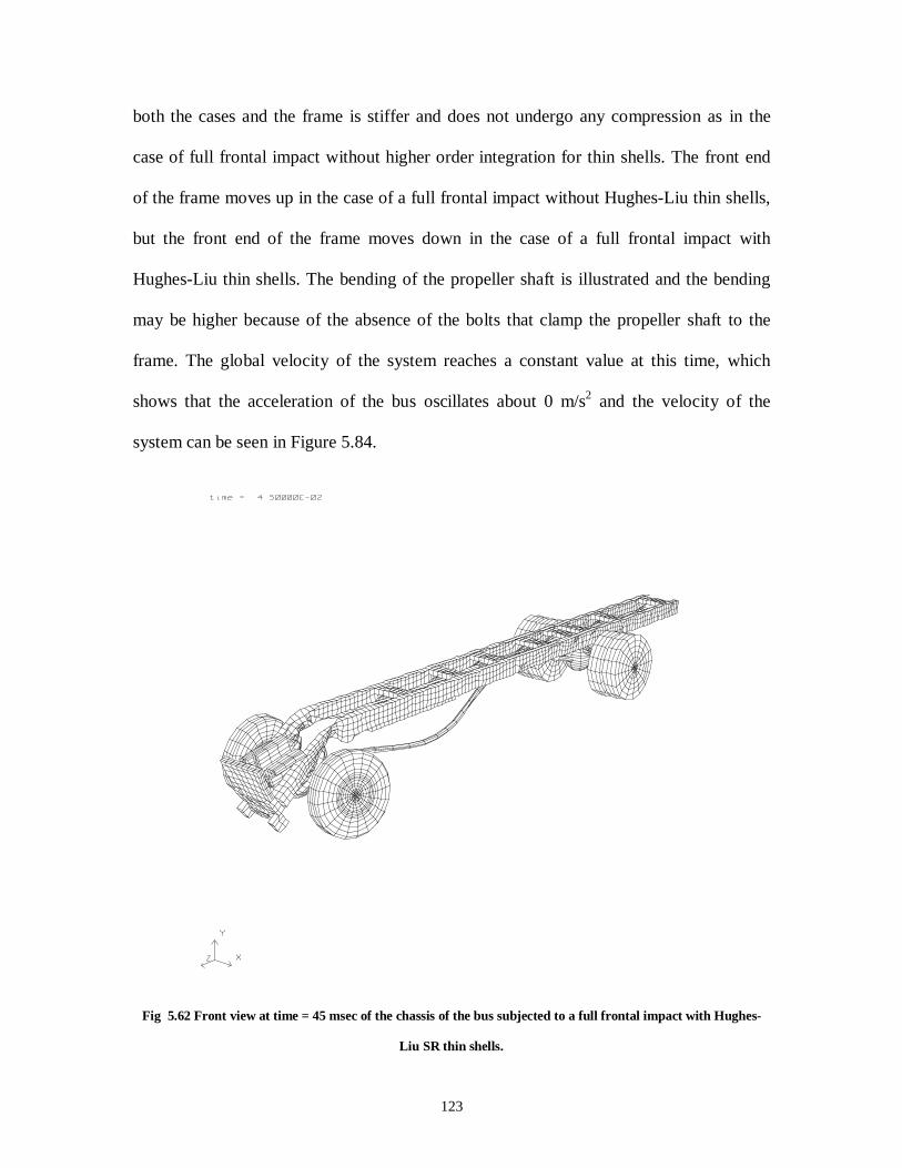
123

both the cases and the frame is stiffer and does not undergo any compression as in the

case of full frontal impact without higher order integration for thin shells. The front end

of the frame moves up in the case of a full frontal impact without Hughes-Liu thin shells,

but the front end of the frame moves down in the case of a full frontal impact with

Hughes-Liu thin shells. The bending of the propeller shaft is illustrated and the bending

may be higher because of the absence of the bolts that clamp the propeller shaft to the

frame. The global velocity of the system reaches a constant value at this time, which

shows that the acceleration of the bus oscillates about 0 m/s2 and the velocity of the

system can be seen in Figure 5.84.

Fig 5.62 Front view at time = 45 msec of the chassis of the bus subjected to a full frontal impact with Hughes-

Liu SR thin shells.

124

Figure 5.63 shows the VonMises stress plot for the frame of the vehicle subjected to

a full frontal impact with Hughes-Liu SR thin shells. The maximum stress in the frame is

18900 MN/m2, which is higher than the yield stress of the material of the frame, and this

can be seen in Appendix C. The maximum stress for a full frontal impact with Hughes-

Liu SR thin shells is higher than the maximum stress that occurs in the frame without

Hughes-Liu SR thin shells as seen in Figures 5.14 and 5.63. However, in both the cases

the maximum stress is higher than the yield stress of the material of the frame. In the case

of a full frontal impact without Hughes-Liu SR thin shells, the front end of the frame

rises up as it hits the rigid wall, which can be seen in Figure 5.14, but in the case of a full

frontal impact with Hughes-Liu SR thin shells the front end of the frame dips down as

seen in Figure 5.63. This behavior of the frame in the first case is due to the presence of

hourglassing in the numerical solution. This is more evident by seeing the deformation of

the front end of the frame in Figure 5.14. The front cross member and the two engine

mounting cross members have also failed at this time. The stresses were plotted for the

shell middle surface for both the cases.

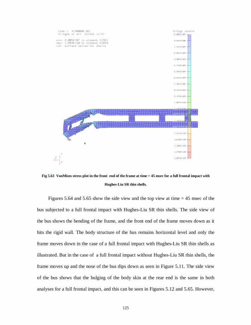
125

Fig 5.63 VonMises stress plot in the front end of the frame at time = 45 msec for a full frontal impact with

Hughes-Liu SR thin shells.

Figures 5.64 and 5.65 show the side view and the top view at time = 45 msec of the

bus subjected to a full frontal impact with Hughes-Liu SR thin shells. The side view of

the bus shows the bending of the frame, and the front end of the frame moves down as it

hits the rigid wall. The body structure of the bus remains horizontal level and only the

frame moves down in the case of a full frontal impact with Hughes-Liu SR thin shells as

illustrated. But in the case of a full frontal impact without Hughes-Liu SR thin shells, the

frame moves up and the nose of the bus dips down as seen in Figure 5.11. The side view

of the bus shows that the bulging of the body skin at the rear end is the same in both

analyses for a full frontal impact, and this can be seen in Figures 5.12 and 5.65. However,

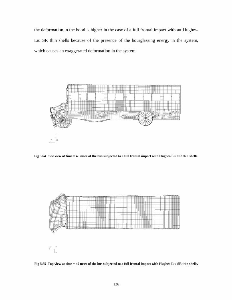
126

the deformation in the hood is higher in the case of a full frontal impact without Hughes-

Liu SR thin shells because of the presence of the hourglassing energy in the system,

which causes an exaggerated deformation in the system.

Fig 5.64 Side view at time = 45 msec of the bus subjected to a full frontal impact with Hughes-Liu SR thin shells.

Fig 5.65 Top view at time = 45 msec of the bus subjected to a full frontal impact with Hughes-Liu SR thin shells.

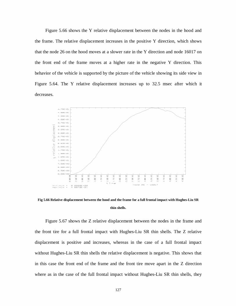
127

Figure 5.66 shows the Y relative displacement between the nodes in the hood and

the frame. The relative displacement increases in the positive Y direction, which shows

that the node 26 on the hood moves at a slower rate in the Y direction and node 16017 on

the front end of the frame moves at a higher rate in the negative Y direction. This

behavior of the vehicle is supported by the picture of the vehicle showing its side view in

Figure 5.64. The Y relative displacement increases up to 32.5 msec after which it

decreases.

Fig 5.66 Relative displacement between the hood and the frame for a full frontal impact with Hughes-Liu SR

thin shells.

Figure 5.67 shows the Z relative displacement between the nodes in the frame and

the front tire for a full frontal impact with Hughes-Liu SR thin shells. The Z relative

displacement is positive and increases, whereas in the case of a full frontal impact

without Hughes-Liu SR thin shells the relative displacement is negative. This shows that

in this case the front end of the frame and the front tire move apart in the Z direction

where as in the case of the full frontal impact without Hughes-Liu SR thin shells, they

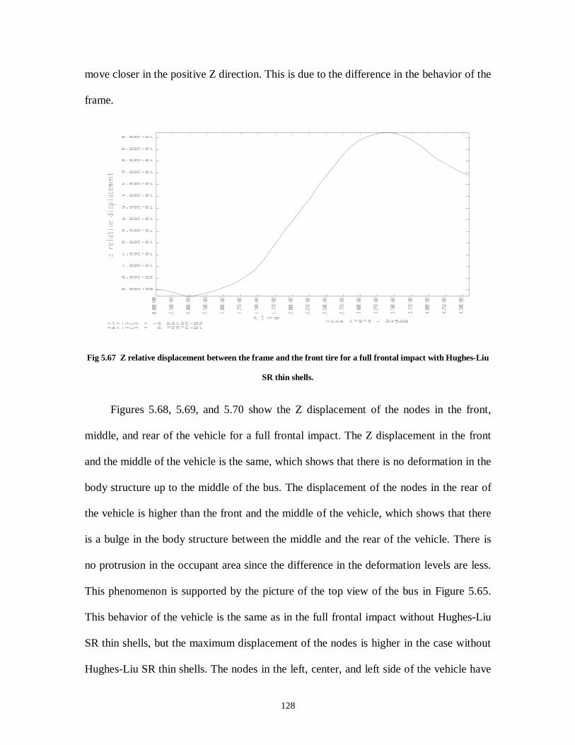
128

move closer in the positive Z direction. This is due to the difference in the behavior of the

frame.

Fig 5.67 Z relative displacement between the frame and the front tire for a full frontal impact with Hughes-Liu

SR thin shells.

Figures 5.68, 5.69, and 5.70 show the Z displacement of the nodes in the front,

middle, and rear of the vehicle for a full frontal impact. The Z displacement in the front

and the middle of the vehicle is the same, which shows that there is no deformation in the

body structure up to the middle of the bus. The displacement of the nodes in the rear of

the vehicle is higher than the front and the middle of the vehicle, which shows that there

is a bulge in the body structure between the middle and the rear of the vehicle. There is

no protrusion in the occupant area since the difference in the deformation levels are less.

This phenomenon is supported by the picture of the top view of the bus in Figure 5.65.

This behavior of the vehicle is the same as in the full frontal impact without Hughes-Liu

SR thin shells, but the maximum displacement of the nodes is higher in the case without

Hughes-Liu SR thin shells. The nodes in the left, center, and left side of the vehicle have

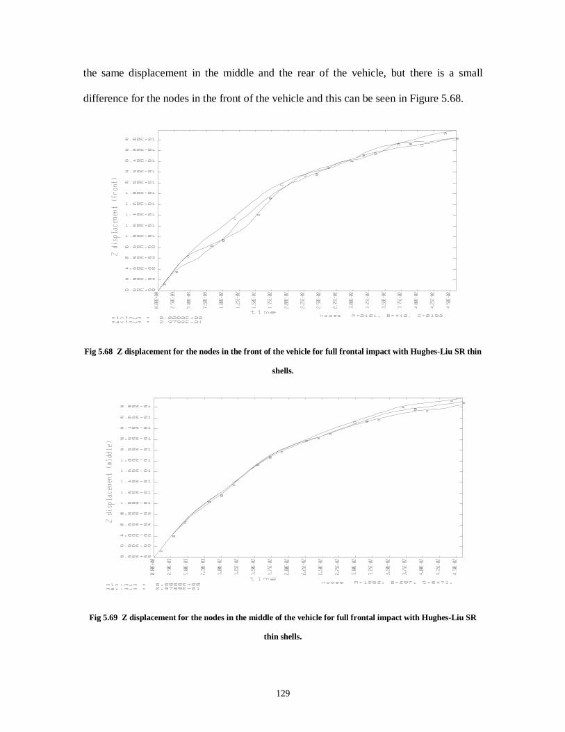
129

the same displacement in the middle and the rear of the vehicle, but there is a small

difference for the nodes in the front of the vehicle and this can be seen in Figure 5.68.

Fig 5.68 Z displacement for the nodes in the front of the vehicle for full frontal impact with Hughes-Liu SR thin

shells.

Fig 5.69 Z displacement for the nodes in the middle of the vehicle for full frontal impact with Hughes-Liu SR

thin shells.

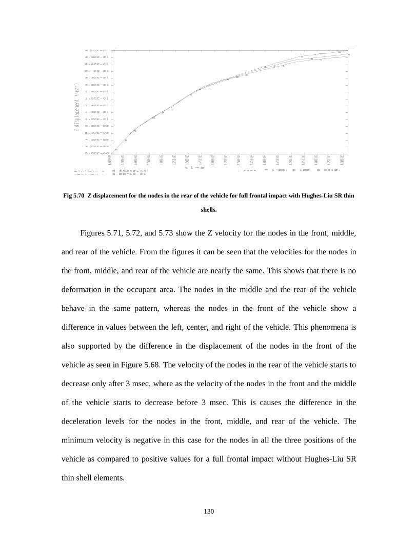
130

Fig 5.70 Z displacement for the nodes in the rear of the vehicle for full frontal impact with Hughes-Liu SR thin

shells.

Figures 5.71, 5.72, and 5.73 show the Z velocity for the nodes in the front, middle,

and rear of the vehicle. From the figures it can be seen that the velocities for the nodes in

the front, middle, and rear of the vehicle are nearly the same. This shows that there is no

deformation in the occupant area. The nodes in the middle and the rear of the vehicle

behave in the same pattern, whereas the nodes in the front of the vehicle show a

difference in values between the left, center, and right of the vehicle. This phenomena is

also supported by the difference in the displacement of the nodes in the front of the

vehicle as seen in Figure 5.68. The velocity of the nodes in the rear of the vehicle starts to

decrease only after 3 msec, where as the velocity of the nodes in the front and the middle

of the vehicle starts to decrease before 3 msec. This is causes the difference in the

deceleration levels for the nodes in the front, middle, and rear of the vehicle. The

minimum velocity is negative in this case for the nodes in all the three positions of the

vehicle as compared to positive values for a full frontal impact without Hughes-Liu SR

thin shell elements.

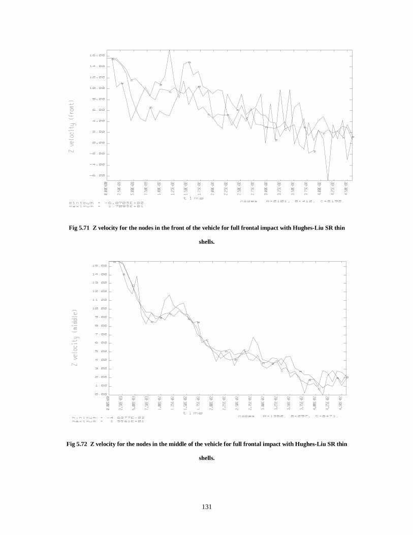
131

Fig 5.71 Z velocity for the nodes in the front of the vehicle for full frontal impact with Hughes-Liu SR thin

shells.

Fig 5.72 Z velocity for the nodes in the middle of the vehicle for full frontal impact with Hughes-Liu SR thin

shells.

132

Fig 5.73 Z velocity for the nodes in the rear of the vehicle for full frontal impact with Hughes-Liu SR thin shells.

Figures 5.74, 5.75, and 5.76 show the Z acceleration of the nodes in the front,

middle, and rear of the vehicle. The deceleration of the nodes in the front of the vehicle is

higher than the deceleration of the nodes in the middle and the rear of the vehicle. The

deceleration of the node in rear of the vehicle is higher than the deceleration of the node

in the middle of the vehicle, which causes the bulging of the outer skin as seen in Figure

5.65. The deceleration of the nodes in the front of the vehicle in this case is higher than

the deceleration of the nodes in the front of the vehicle without Hughes-Liu SR thin

shells. The Z acceleration of the nodes in the front shows high oscillations about zero,

whereas the oscillations of the nodes in the middle and the rear of the vehicle are less.

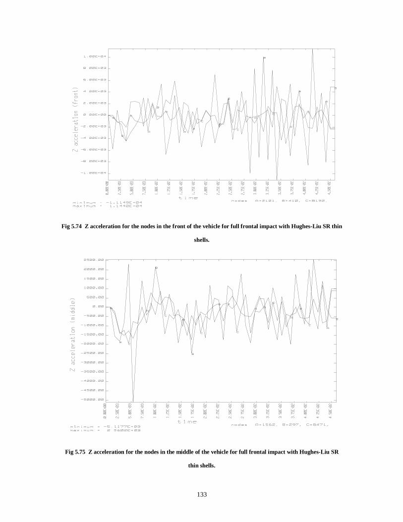
133

Fig 5.74 Z acceleration for the nodes in the front of the vehicle for full frontal impact with Hughes-Liu SR thin

shells.

Fig 5.75 Z acceleration for the nodes in the middle of the vehicle for full frontal impact with Hughes-Liu SR

thin shells.

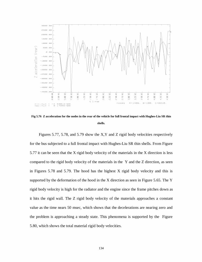
134

Fig 5.76 Z acceleration for the nodes in the rear of the vehicle for full frontal impact with Hughes-Liu SR thin

shells.

Figures 5.77, 5.78, and 5.79 show the X,Y and Z rigid body velocities respectively

for the bus subjected to a full frontal impact with Hughes-Liu SR thin shells. From Figure

5.77 it can be seen that the X rigid body velocity of the materials in the X direction is less

compared to the rigid body velocity of the materials in the Y and the Z direction, as seen

in Figures 5.78 and 5.79. The hood has the highest X rigid body velocity and this is

supported by the deformation of the hood in the X direction as seen in Figure 5.65. The Y

rigid body velocity is high for the radiator and the engine since the frame pitches down as

it hits the rigid wall. The Z rigid body velocity of the materials approaches a constant

value as the time nears 50 msec, which shows that the decelerations are nearing zero and

the problem is approaching a steady state. This phenomena is supported by the Figure

5.80, which shows the total material rigid body velocities.

135

Fig 5.77 X rigid body velocities of materials for a full frontal impact with Hughes-Liu SR thin shells.

Fig 5.78 Y rigid body velocities of materials for a full frontal impact with Hughes-Liu SR thin shells.

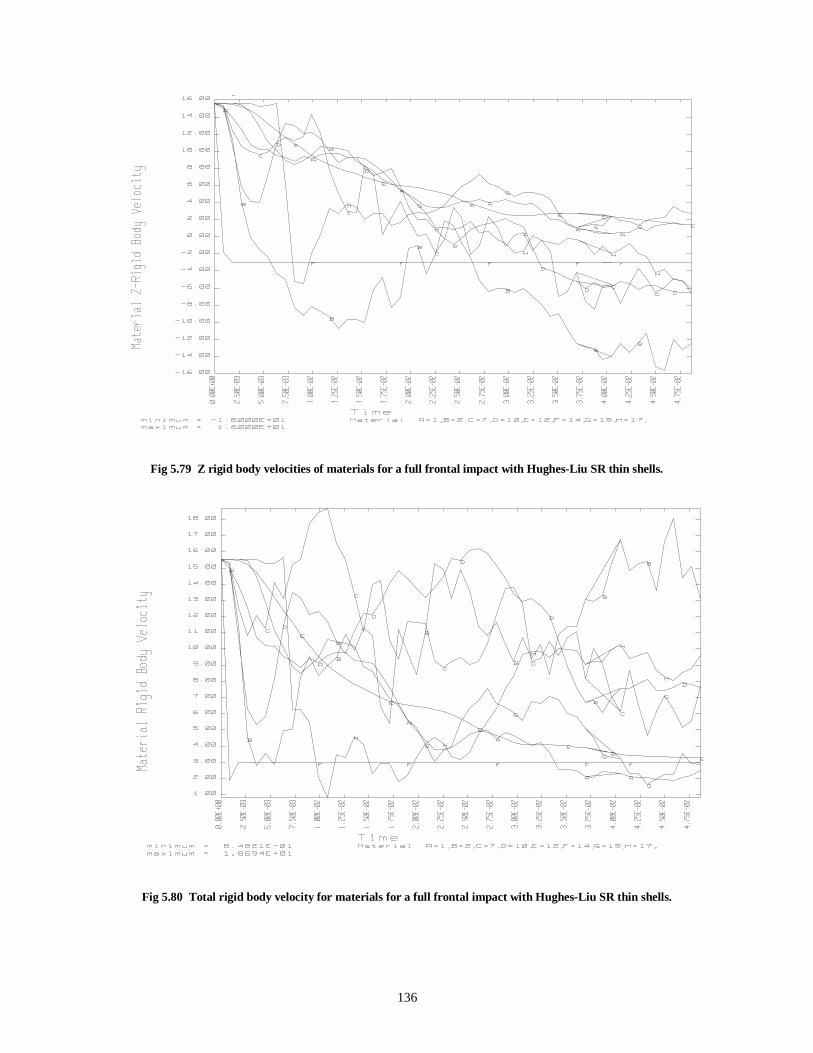
136

Fig 5.79 Z rigid body velocities of materials for a full frontal impact with Hughes-Liu SR thin shells.

Fig 5.80 Total rigid body velocity for materials for a full frontal impact with Hughes-Liu SR thin shells.

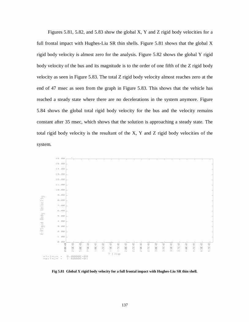
137

Figures 5.81, 5.82, and 5.83 show the global X, Y and Z rigid body velocities for a

full frontal impact with Hughes-Liu SR thin shells. Figure 5.81 shows that the global X

rigid body velocity is almost zero for the analysis. Figure 5.82 shows the global Y rigid

body velocity of the bus and its magnitude is to the order of one fifth of the Z rigid body

velocity as seen in Figure 5.83. The total Z rigid body velocity almost reaches zero at the

end of 47 msec as seen from the graph in Figure 5.83. This shows that the vehicle has

reached a steady state where there are no decelerations in the system anymore. Figure

5.84 shows the global total rigid body velocity for the bus and the velocity remains

constant after 35 msec, which shows that the solution is approaching a steady state. The

total rigid body velocity is the resultant of the X, Y and Z rigid body velocities of the

system.

Fig 5.81 Global X rigid body velocity for a full frontal impact with Hughes-Liu SR thin shell.

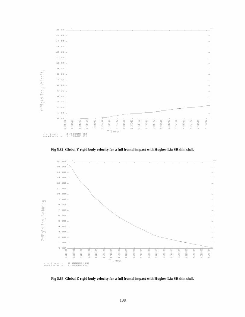
138

Fig 5.82 Global Y rigid body velocity for a full frontal impact with Hughes-Liu SR thin shell.

Fig 5.83 Global Z rigid body velocity for a full frontal impact with Hughes-Liu SR thin shell.

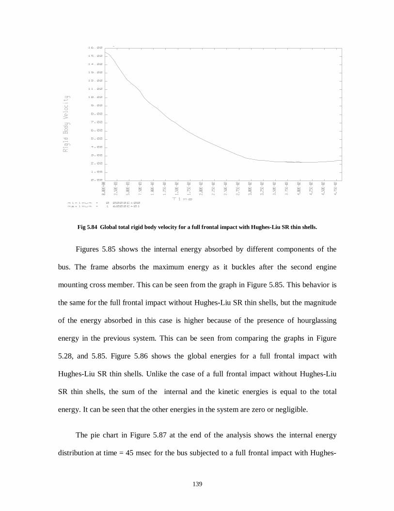
139

Fig 5.84 Global total rigid body velocity for a full frontal impact with Hughes-Liu SR thin shells.

Figures 5.85 shows the internal energy absorbed by different components of the

bus. The frame absorbs the maximum energy as it buckles after the second engine

mounting cross member. This can be seen from the graph in Figure 5.85. This behavior is

the same for the full frontal impact without Hughes-Liu SR thin shells, but the magnitude

of the energy absorbed in this case is higher because of the presence of hourglassing

energy in the previous system. This can be seen from comparing the graphs in Figure

5.28, and 5.85. Figure 5.86 shows the global energies for a full frontal impact with

Hughes-Liu SR thin shells. Unlike the case of a full frontal impact without Hughes-Liu

SR thin shells, the sum of the internal and the kinetic energies is equal to the total

energy. It can be seen that the other energies in the system are zero or negligible.

The pie chart in Figure 5.87 at the end of the analysis shows the internal energy

distribution at time = 45 msec for the bus subjected to a full frontal impact with Hughes-

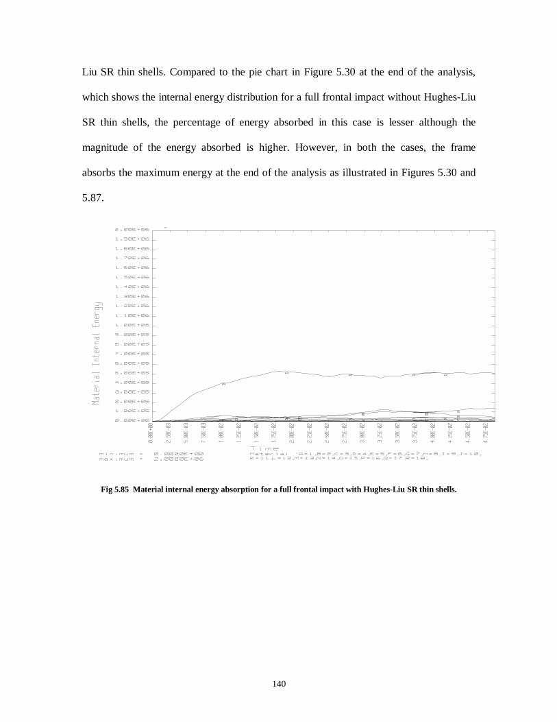
140

Liu SR thin shells. Compared to the pie chart in Figure 5.30 at the end of the analysis,

which shows the internal energy distribution for a full frontal impact without Hughes-Liu

SR thin shells, the percentage of energy absorbed in this case is lesser although the

magnitude of the energy absorbed is higher. However, in both the cases, the frame

absorbs the maximum energy at the end of the analysis as illustrated in Figures 5.30 and

5.87.

Fig 5.85 Material internal energy absorption for a full frontal impact with Hughes-Liu SR thin shells.

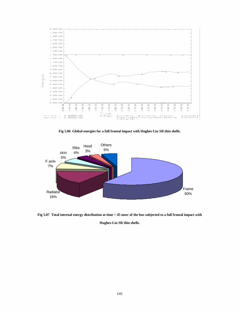
141

Fig 5.86 Global energies for a full frontal impact with Hughes-Liu SR thin shells.

Frame60%Radiator

16%

F.axle7%

skin5%

Ribs4%

Hood3%

Others5%

Fig 5.87 Total internal energy distribution at time = 45 msec of the bus subjected to a full frontal impact with

Hughes-Liu SR thin shells.

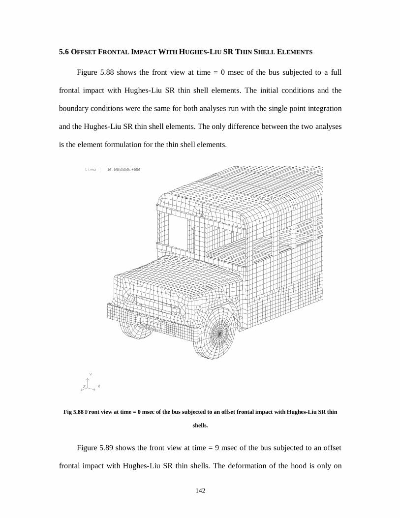
142

5.6 OFFSET FRONTAL IMPACT WITH HUGHES-LIU SR THIN SHELL ELEMENTS

Figure 5.88 shows the front view at time = 0 msec of the bus subjected to a full

frontal impact with Hughes-Liu SR thin shell elements. The initial conditions and the

boundary conditions were the same for both analyses run with the single point integration

and the Hughes-Liu SR thin shell elements. The only difference between the two analyses

is the element formulation for the thin shell elements.

Fig 5.88 Front view at time = 0 msec of the bus subjected to an offset frontal impact with Hughes-Liu SR thin

shells.


frontal impact with Hughes-Liu SR thin shells. The deformation of the hood is only on

143

one side of the hood as illustrated. The deformation at this time state is the same for the

both cases with and without Hughes-Liu SR thin shells because of the absence of

hourglassing energy in the initial stages of the analysis. This can be seen by comparing

Figures 5.88 and 5.31. Since the principal direction of the impact force is offset from the

line of symmetry of the hood, the front axle rotates and the right wheel (door side) moves

in the negative Z direction. This can be seen from the graph in Figure 5.97.


shells.


frontal impact with Hughes-Liu SR thin shell elements. The difference in Z displacement

144

between the nodes in the right and the left tire increases, which shows the rotation of the

front axle and in this case, the vehicle behaves in the same way as the offset frontal

collision without Hughes-Liu SR thin shell elements. The velocity of the vehicle lessens

and hence the kinetic energy of the system is reduced. The internal energy absorbed by

the parts in the front end of the vehicle increases as the kinetic energy decreases and this

can be seen in Figure 5.114.


shells.


frontal impact with Hughes-Liu SR thin shell elements. The front tires move in the

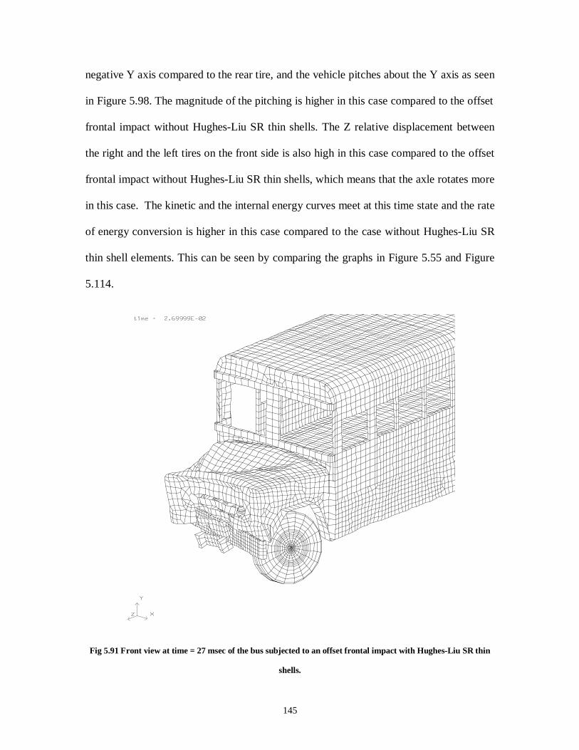
145

negative Y axis compared to the rear tire, and the vehicle pitches about the Y axis as seen

in Figure 5.98. The magnitude of the pitching is higher in this case compared to the offset

frontal impact without Hughes-Liu SR thin shells. The Z relative displacement between

the right and the left tires on the front side is also high in this case compared to the offset

frontal impact without Hughes-Liu SR thin shells, which means that the axle rotates more

in this case. The kinetic and the internal energy curves meet at this time state and the rate

of energy conversion is higher in this case compared to the case without Hughes-Liu SR

thin shell elements. This can be seen by comparing the graphs in Figure 5.55 and Figure

5.114.


shells.

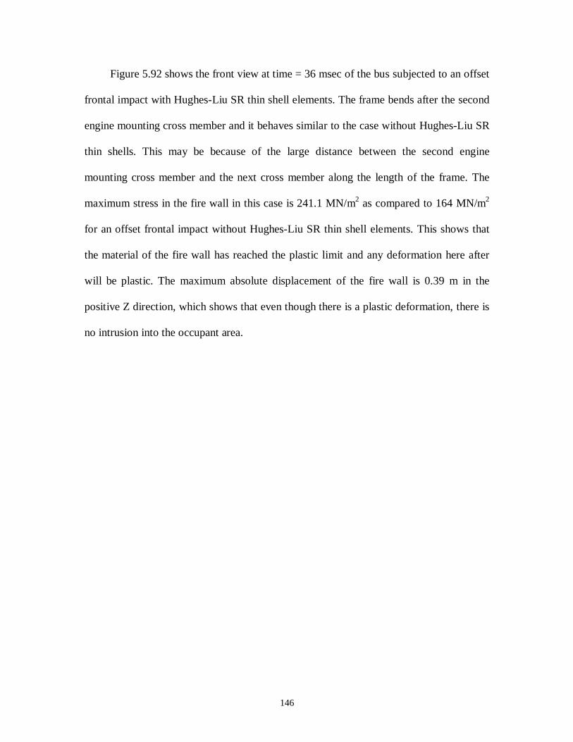
146


frontal impact with Hughes-Liu SR thin shell elements. The frame bends after the second

engine mounting cross member and it behaves similar to the case without Hughes-Liu SR

thin shells. This may be because of the large distance between the second engine

mounting cross member and the next cross member along the length of the frame. The

maximum stress in the fire wall in this case is 241.1 MN/m2 as compared to 164 MN/m2

for an offset frontal impact without Hughes-Liu SR thin shell elements. This shows that

the material of the fire wall has reached the plastic limit and any deformation here after

will be plastic. The maximum absolute displacement of the fire wall is 0.39 m in the

positive Z direction, which shows that even though there is a plastic deformation, there is

no intrusion into the occupant area.

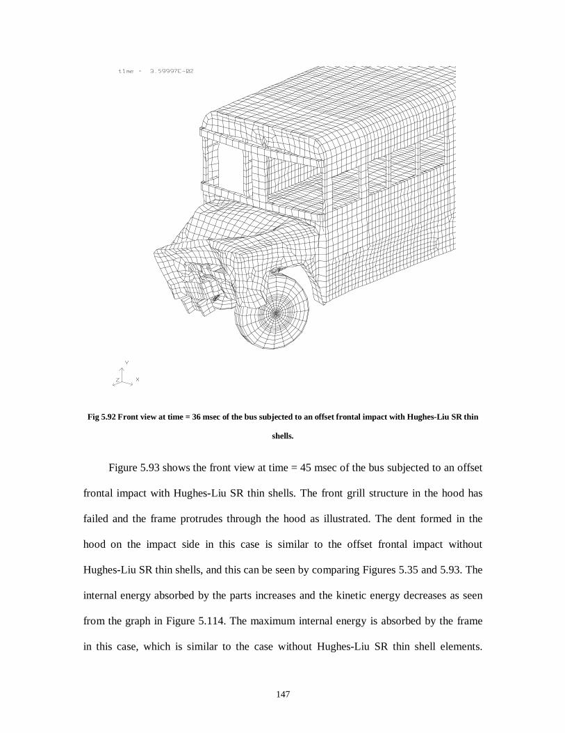
147


shells.


frontal impact with Hughes-Liu SR thin shells. The front grill structure in the hood has

failed and the frame protrudes through the hood as illustrated. The dent formed in the

hood on the impact side in this case is similar to the offset frontal impact without

Hughes-Liu SR thin shells, and this can be seen by comparing Figures 5.35 and 5.93. The

internal energy absorbed by the parts increases and the kinetic energy decreases as seen

from the graph in Figure 5.114. The maximum internal energy is absorbed by the frame

in this case, which is similar to the case without Hughes-Liu SR thin shell elements.

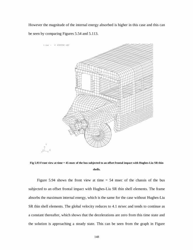
148

However the magnitude of the internal energy absorbed is higher in this case and this can

be seen by comparing Figures 5.54 and 5.113.


shells.

Figure 5.94 shows the front view at time = 54 msec of the chassis of the bus

subjected to an offset frontal impact with Hughes-Liu SR thin shell elements. The frame

absorbs the maximum internal energy, which is the same for the case without Hughes-Liu

SR thin shell elements. The global velocity reduces to 4.1 m/sec and tends to continue as

a constant thereafter, which shows that the decelerations are zero from this time state and

the solution is approaching a steady state. This can be seen from the graph in Figure

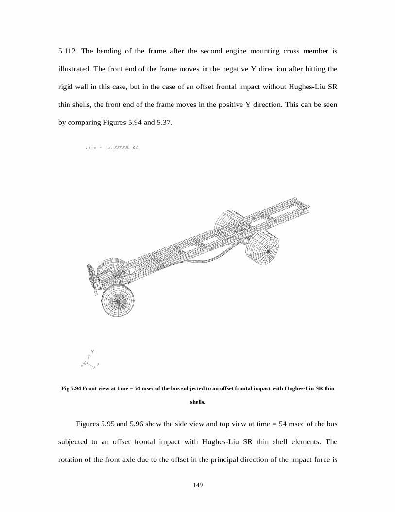
149

5.112. The bending of the frame after the second engine mounting cross member is

illustrated. The front end of the frame moves in the negative Y direction after hitting the

rigid wall in this case, but in the case of an offset frontal impact without Hughes-Liu SR

thin shells, the front end of the frame moves in the positive Y direction. This can be seen

by comparing Figures 5.94 and 5.37.


shells.

Figures 5.95 and 5.96 show the side view and top view at time = 54 msec of the bus

subjected to an offset frontal impact with Hughes-Liu SR thin shell elements. The

rotation of the front axle due to the offset in the principal direction of the impact force is

150

illustrated. The bending of the propeller shaft is also seen in the figure. The side view

shows the deformation on only one side of the hood due to an offset in the impact force.

Fig 5.95 Side view at time = 54 msec of the bus subjected to an offset frontal impact with Hughes-Liu SR thin

shells.

Fig 5.96 Top view at time = 54 msec of the bus subjected to an offset frontal impact with Hughes-Liu SR thin

shells.

151

Figure 5.97 shows the relative displacement between the right wheel and the left

wheel for an offset frontal impact with Hughes-Liu SR thin shell elements. The relative

displacement continuously increases, which shows that the front axle rotates about the Y

axis. The maximum relative displacement is 1.4 m in this case as compared to 0.65 m for

an offset frontal impact without Hughes-Liu SR thin shell elements. This shows that the

rotation of the front axle is higher in this case. Figure 5.98 shows the relative

displacement between the front tire and the rear tire. The relative displacement

continuously increases, which shows the pitching of the vehicle. The maximum relative

displacement is 0.16 m in this case and this is higher than the case for an offset frontal

impact without Hughes-Liu SR thin shell elements since the vehicle starts pitching only

after 65 msec.

Fig 5.97 Relative displacement between the right wheel and the left wheel (axle rotation) for an offset frontal

impact with Hughes-Liu SR thin shell elements.

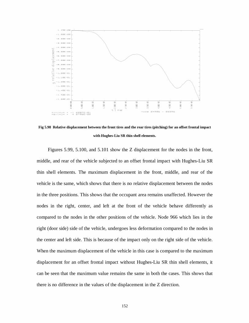
152

Fig 5.98 Relative displacement between the front tires and the rear tires (pitching) for an offset frontal impact

with Hughes-Liu SR thin shell elements.

Figures 5.99, 5.100, and 5.101 show the Z displacement for the nodes in the front,

middle, and rear of the vehicle subjected to an offset frontal impact with Hughes-Liu SR

thin shell elements. The maximum displacement in the front, middle, and rear of the

vehicle is the same, which shows that there is no relative displacement between the nodes

in the three positions. This shows that the occupant area remains unaffected. However the

nodes in the right, center, and left at the front of the vehicle behave differently as

compared to the nodes in the other positions of the vehicle. Node 966 which lies in the

right (door side) side of the vehicle, undergoes less deformation compared to the nodes in

the center and left side. This is because of the impact only on the right side of the vehicle.

When the maximum displacement of the vehicle in this case is compared to the maximum

displacement for an offset frontal impact without Hughes-Liu SR thin shell elements, it

can be seen that the maximum value remains the same in both the cases. This shows that

there is no difference in the values of the displacement in the Z direction.

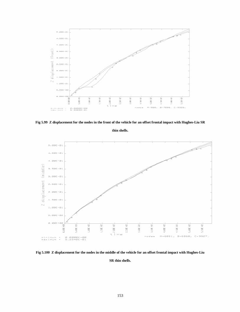
153

Fig 5.99 Z displacement for the nodes in the front of the vehicle for an offset frontal impact with Hughes-Liu SR

thin shells.

Fig 5.100 Z displacement for the nodes in the middle of the vehicle for an offset frontal impact with Hughes-Liu

SR thin shells.

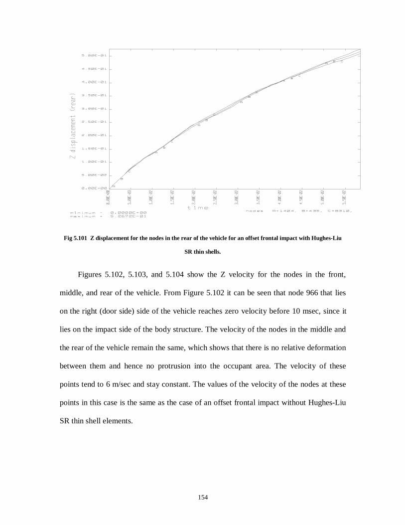
154

Fig 5.101 Z displacement for the nodes in the rear of the vehicle for an offset frontal impact with Hughes-Liu

SR thin shells.

Figures 5.102, 5.103, and 5.104 show the Z velocity for the nodes in the front,

middle, and rear of the vehicle. From Figure 5.102 it can be seen that node 966 that lies

on the right (door side) side of the vehicle reaches zero velocity before 10 msec, since it

lies on the impact side of the body structure. The velocity of the nodes in the middle and

the rear of the vehicle remain the same, which shows that there is no relative deformation

between them and hence no protrusion into the occupant area. The velocity of these

points tend to 6 m/sec and stay constant. The values of the velocity of the nodes at these

points in this case is the same as the case of an offset frontal impact without Hughes-Liu

SR thin shell elements.

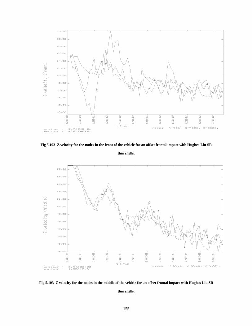
155

Fig 5.102 Z velocity for the nodes in the front of the vehicle for an offset frontal impact with Hughes-Liu SR

thin shells.

Fig 5.103 Z velocity for the nodes in the middle of the vehicle for an offset frontal impact with Hughes-Liu SR

thin shells.

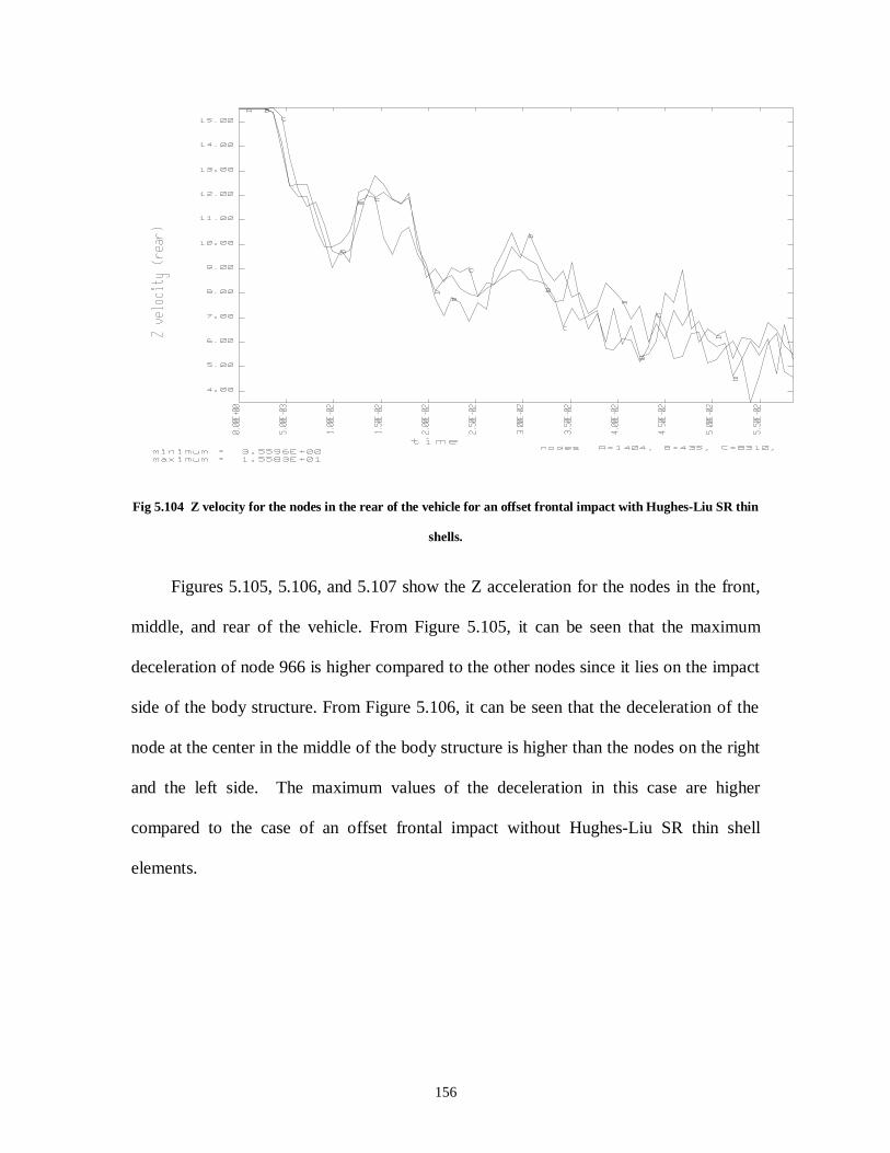
156

Fig 5.104 Z velocity for the nodes in the rear of the vehicle for an offset frontal impact with Hughes-Liu SR thin

shells.

Figures 5.105, 5.106, and 5.107 show the Z acceleration for the nodes in the front,

middle, and rear of the vehicle. From Figure 5.105, it can be seen that the maximum

deceleration of node 966 is higher compared to the other nodes since it lies on the impact

side of the body structure. From Figure 5.106, it can be seen that the deceleration of the

node at the center in the middle of the body structure is higher than the nodes on the right

and the left side. The maximum values of the deceleration in this case are higher

compared to the case of an offset frontal impact without Hughes-Liu SR thin shell

elements.

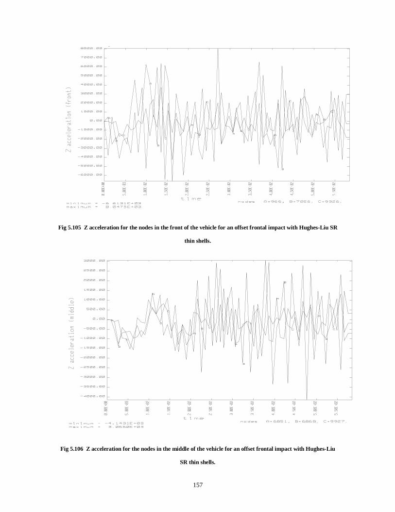
157

Fig 5.105 Z acceleration for the nodes in the front of the vehicle for an offset frontal impact with Hughes-Liu SR

thin shells.

Fig 5.106 Z acceleration for the nodes in the middle of the vehicle for an offset frontal impact with Hughes-Liu

SR thin shells.

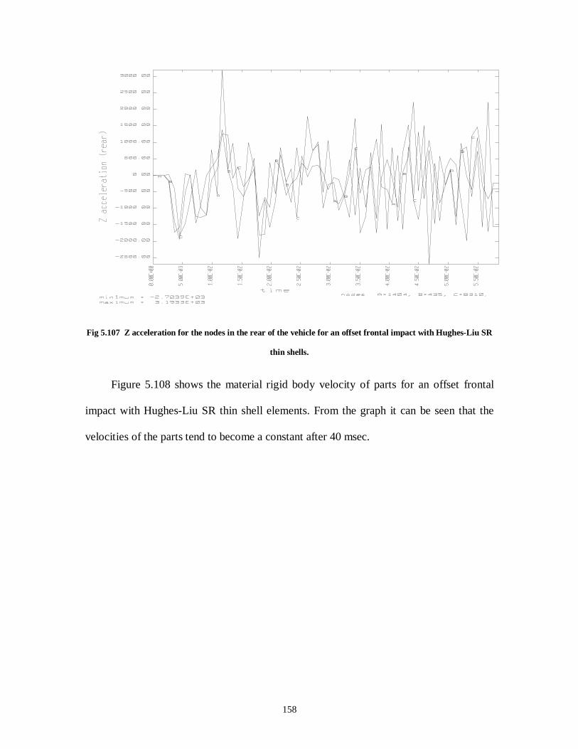
158

Fig 5.107 Z acceleration for the nodes in the rear of the vehicle for an offset frontal impact with Hughes-Liu SR

thin shells.

Figure 5.108 shows the material rigid body velocity of parts for an offset frontal

impact with Hughes-Liu SR thin shell elements. From the graph it can be seen that the

velocities of the parts tend to become a constant after 40 msec.

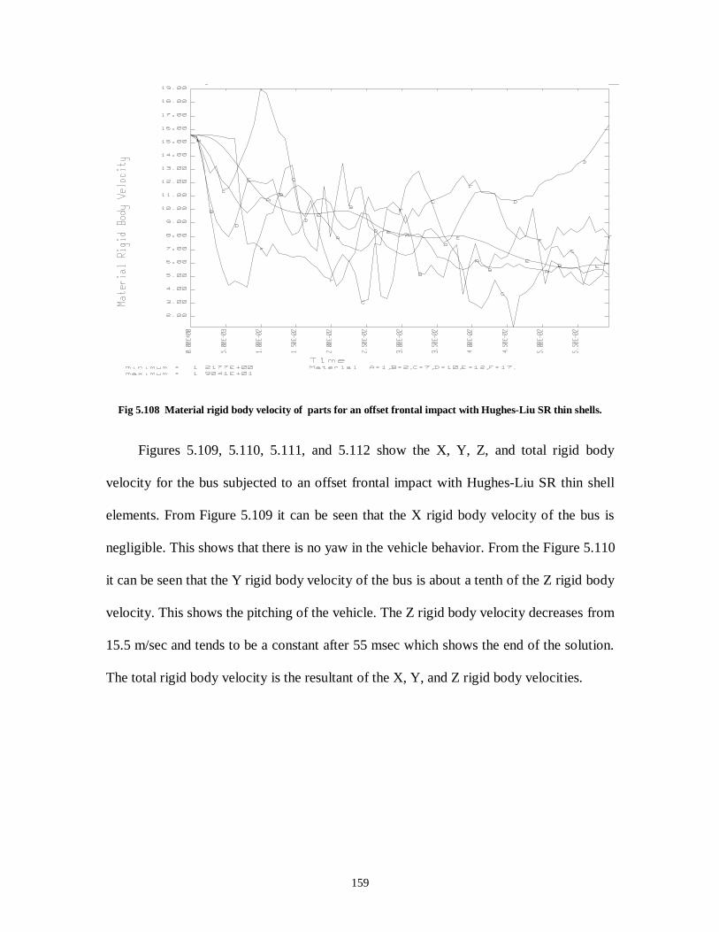
159

Fig 5.108 Material rigid body velocity of parts for an offset frontal impact with Hughes-Liu SR thin shells.

Figures 5.109, 5.110, 5.111, and 5.112 show the X, Y, Z, and total rigid body

velocity for the bus subjected to an offset frontal impact with Hughes-Liu SR thin shell

elements. From Figure 5.109 it can be seen that the X rigid body velocity of the bus is

negligible. This shows that there is no yaw in the vehicle behavior. From the Figure 5.110

it can be seen that the Y rigid body velocity of the bus is about a tenth of the Z rigid body

velocity. This shows the pitching of the vehicle. The Z rigid body velocity decreases from

15.5 m/sec and tends to be a constant after 55 msec which shows the end of the solution.

The total rigid body velocity is the resultant of the X, Y, and Z rigid body velocities.

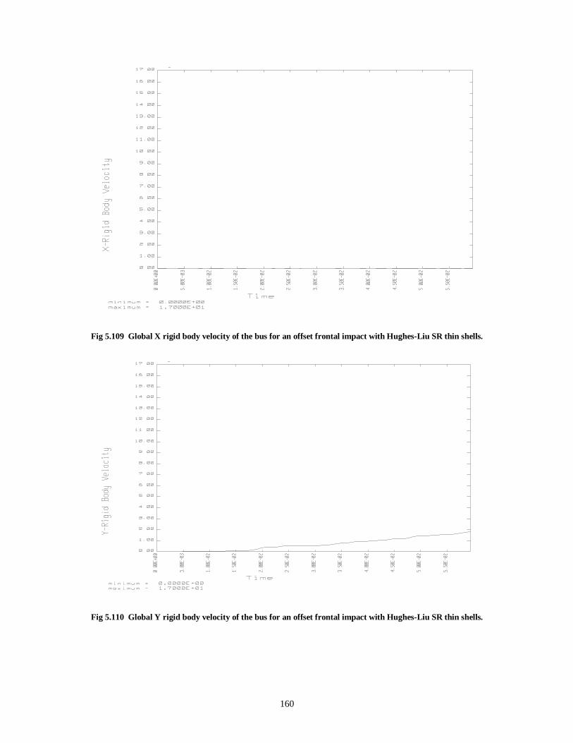
160

Fig 5.109 Global X rigid body velocity of the bus for an offset frontal impact with Hughes-Liu SR thin shells.

Fig 5.110 Global Y rigid body velocity of the bus for an offset frontal impact with Hughes-Liu SR thin shells.

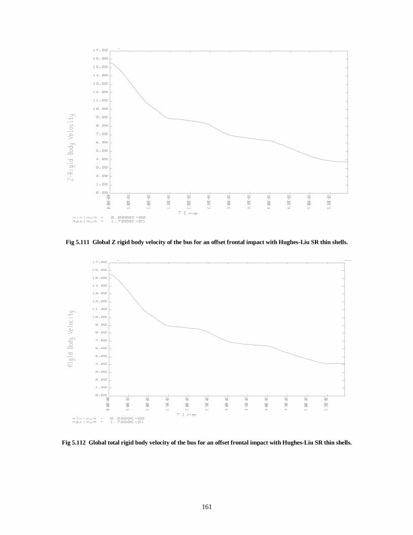
161

Fig 5.111 Global Z rigid body velocity of the bus for an offset frontal impact with Hughes-Liu SR thin shells.

Fig 5.112 Global total rigid body velocity of the bus for an offset frontal impact with Hughes-Liu SR thin shells.

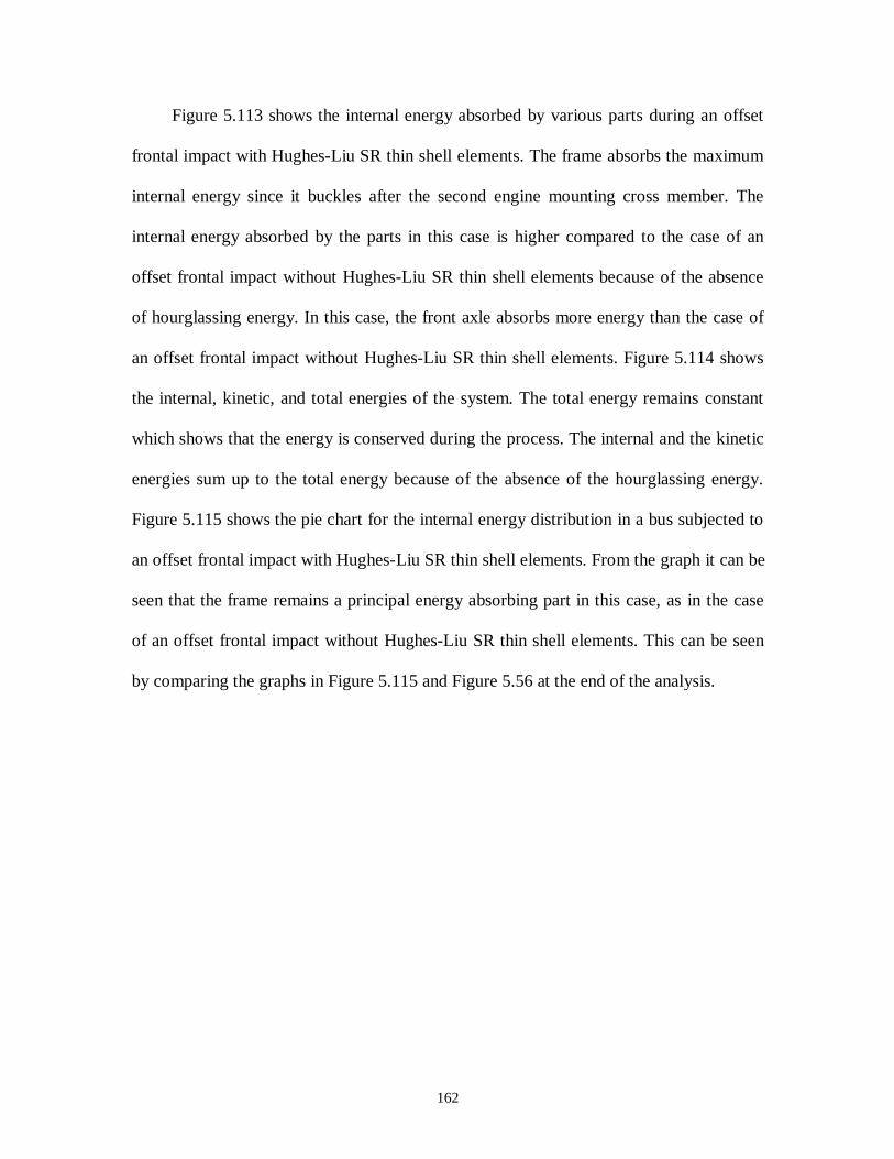
162

Figure 5.113 shows the internal energy absorbed by various parts during an offset

frontal impact with Hughes-Liu SR thin shell elements. The frame absorbs the maximum

internal energy since it buckles after the second engine mounting cross member. The

internal energy absorbed by the parts in this case is higher compared to the case of an

offset frontal impact without Hughes-Liu SR thin shell elements because of the absence

of hourglassing energy. In this case, the front axle absorbs more energy than the case of

an offset frontal impact without Hughes-Liu SR thin shell elements. Figure 5.114 shows

the internal, kinetic, and total energies of the system. The total energy remains constant

which shows that the energy is conserved during the process. The internal and the kinetic

energies sum up to the total energy because of the absence of the hourglassing energy.

Figure 5.115 shows the pie chart for the internal energy distribution in a bus subjected to

an offset frontal impact with Hughes-Liu SR thin shell elements. From the graph it can be

seen that the frame remains a principal energy absorbing part in this case, as in the case

of an offset frontal impact without Hughes-Liu SR thin shell elements. This can be seen

by comparing the graphs in Figure 5.115 and Figure 5.56 at the end of the analysis.

163

Fig 5.113 Material internal energy of parts for an offset frontal impact with Hughes-Liu SR thin shells.

Fig 5.114 Internal , kinetic and total energies for an offset frontal impact with Hughes-Liu SR thin shells.

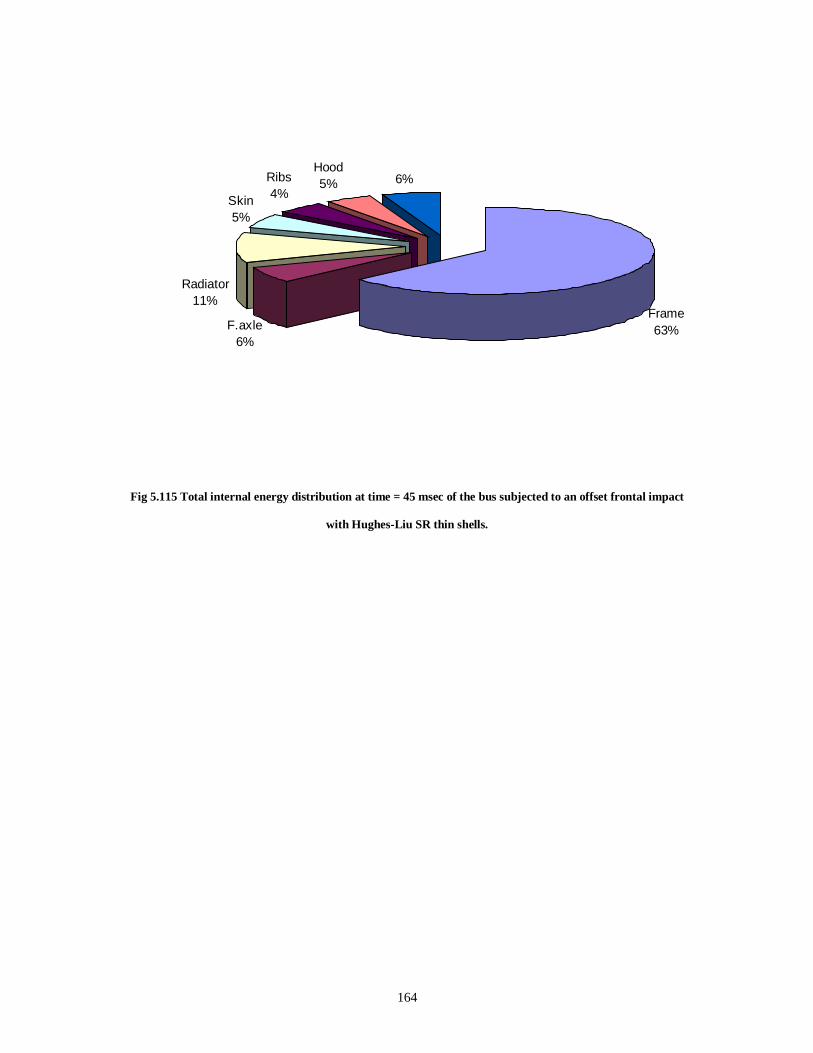
164

Frame63%F.axle

6%

Radiator11%

Skin5%

Ribs4%

Hood5% 6%

Fig 5.115 Total internal energy distribution at time = 45 msec of the bus subjected to an offset frontal impact

with Hughes-Liu SR thin shells.

165

CHAPTER 6 –CONCLUSIONS AND RECOMMENDATIONS

6.1 CONCLUSIONS

The finite element model of the bus was developed using I-DEAS Master Series

software. Quadrilateral thin shell elements were used for sheet metal components and

solid elements were used for the solid blocks to mesh the parts of the bus. The explicit

time integration method was used to solve the model with eight-point integration for solid

elements and single-point integration for thin shell elements. The single-point integration

gives rise to the zero energy modes which produce the hourglass mode shapes. Since

eight-point integration was used for solid elements, hourglassing was completely

eliminated in all the solid elements and the hourglassing energy present in the energy

balance is only from the thin shell elements. So a higher order integration for the thin

shell elements was used which increased the solution time by five times the single-point

integration. To avoid the hourglass energy for the thin shell elements, Hughes-Liu

elements with Selective-Reduced integration were used. These elements are integrated

using 2 X 2 Gaussian quadrature in the plane, and these elements are extremely useful in

places where hourglassing is a problem.

Contact type 3 in LS-DYNA3D was defined between the surfaces of the front end

components of the bus, which gave rise to hourglassing energy. This resulted in the

continuous increase of the total energy in the system untill the end of the analysis. The

contact type 3 was changed to contact type 4 and contact type 5 in LS-DYNA3D. Contact

type 4 creates contact between the folding surfaces of the same part or material. Contact

type 5 creates contact between the nodes of a slave surface to the element face on the

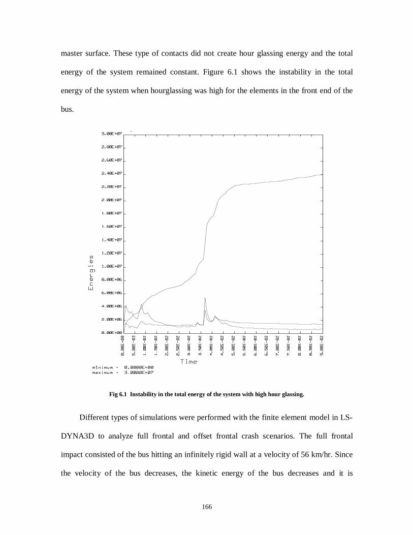
166

master surface. These type of contacts did not create hour glassing energy and the total

energy of the system remained constant. Figure 6.1 shows the instability in the total

energy of the system when hourglassing was high for the elements in the front end of the

bus.

Fig 6.1 Instability in the total energy of the system with high hour glassing.

Different types of simulations were performed with the finite element model in LS-

DYNA3D to analyze full frontal and offset frontal crash scenarios. The full frontal

impact consisted of the bus hitting an infinitely rigid wall at a velocity of 56 km/hr. Since

the velocity of the bus decreases, the kinetic energy of the bus decreases and it is

167

converted into material internal energy. The general characteristics like the displacement,

velocity, and acceleration of the parts provide an indication of the deformation undergone

by the parts of the bus.

The frame absorbs the maximum amount of kinetic energy converted as material

internal energy for a full frontal impact. The occupant area in the bus lies inside the rib

structure and it is covered by the inner skin and the outer skin. In a full frontal impact, the

occupant area remains unaffected and the deformation of the front end components are

only up to the fire wall of the bus. The deformation in the fire wall causing an intrusion

into the driver’s compartment is small. There is a small deformation in the body skin of

the bus and the two layers of skin do not intrude but instead bulge outwards, which is not

harmful to the occupants. The vehicle rotates about the X axis, which is called the

pitching of the vehicle. This may cause the occupants in the bus to be thrown out of their

seats and hit the back of the front seat, which might result in serious injuries. When the

analysis was run with Hughes-Liu SR thin shell elements, the body structure pitching was

less, and the pitching of the frame was high.

The offset frontal impact consisted of only one side of the bus hitting an infinitely

rigid wall at a velocity of 56 km/hr. Only the right half (door way) of the bus hits the

rigid wall and decelerates. The kinetic energy of the bus is converted into material

internal energy since the kinetic energy decreases. The frame absorbs the maximum

energy in this case and it buckles after the second engine mounting cross member. This

deformation in the frame absorbs the maximum energy and protects the impact force

from being transmitted to the occupant area. The front axle rotates and the right wheel

hits the fire wall. This might cause a deformation in the body structure near the doorway

168

of the bus. The energy absorbed by the rib structure that protects the occupant area is

small compared to the front end components, which shows that the deformation is less in

the bus body and there is no intrusion of any components of the bus into the occupant

area.

If the impact had been simulated for the driver side half of the bus, the left wheel

may have intruded into the driver occupant area after the fire wall. The vehicle pitches in

this case also, which shows that the occupants could be harmed due to the pitching of the

vehicle and the occupants being thrown out of their seats. In this case when the analysis

was run with Hughes-Liu SR thin shell elements, the pitching was high compared to the

analysis without Hughes-Liu SR thin shell elements.

Two simulation runs were made for the full frontal and the offset frontal crash

scenarios, one without Hughes-Liu SR thin shell elements and the other with Hughes-Liu

SR thin shell elements. The analysis without Hughes-Liu SR thin shell and with the

default LS-DYNA3D shell element formulation, had hourglassing energy and the sum of

the internal and the kinetic energies was not equal to the total energies. The second case,

with the Hughes-Liu SR thin shell element formulation, had zero hourglassing energy

and the sum of the internal and the kinetic energies was equal to the total energy. The

kinetic energy decreases from the beginning of the solution and the internal energy

increases and both the curves meet at exactly half the total energy.

The behavior of the vehicles in both cases was different: however, the frame

remained as the principal energy absorbing part in the impact for the full frontal and the

offset frontal impact with and without Hughes-Liu SR thin shell elements. So higher

169

order integration for the thin shell elements with Hughes-Liu thin shell formulation is

recommended in this case. The frame plays an important role in the full frontal and the

offset frontal impact as it buckles after the second engine mounting cross member and

absorbs a major chunk of the kinetic energy as internal energy. Since it is evident from

the results that the frame plays an important role in the full frontal and the offset frontal

impacts, modeling the frame is recommended for the frontal crash impact scenarios. The

time taken for the solution with Hughes-Liu SR thin shells is at least five times the time

taken for the analysis without Hughes-Liu SR thin shell elements.

This thesis demonstrates the ability of numerical simulation to simulate two

different scenarios of impact. This project studies the deformation behavior of the vehicle

and its effect on the occupants of the bus. The deformation on the bus body structure

would help to study the intrusion of the bus components in the occupant area in the event

of a crash. The model is a design tool that can be used to study the effects of changing

component design. These changes could include lowering the center of gravity and/or

changing component materials (steel to aluminum). The model could also be used to

examine the effects of changing the frame rail design to prevent pitching of the vehicle in

a frontal collision. The validation and the accuracy of the results obtained from the

simulation have to be checked. The National Highway Traffic Safety Administration does

not have adequate data that could correspond to the crashworthiness of a Type C school

bus. This emphasizes the need for tests to be performed on a school bus to study and

compare the behavior of the school bus against the simulation results. The changes that

can be incorporated in the model is the reduction in the number of elements for the tire

since the tire takes more number of elements and hence more solution time. Also changes

170

could be incorporated by accounting for the changes in material properties during the

steel forming process as done by Kaufman and Gaines22.

The side impact and rear impact could be simulated by modeling a rigid wall to the

side and the rear of the bus respectively. Since the mesh density for the all the

components in the bus is close enough to study the deformation shapes, the same finite

element model can be used without any changes. The frame plays an important role in

absorbing as much energy as possible during the crash event, which emphasizes the need

of modeling the frame for frontal impacts. The designer could use the output from this

work for an improvement in design of the school buses.

171

CHAPTER – 8 REFERENCES

1Frank F. Monasa and William Mcguire, “Collapse Analysis of Bus Body Structures

using Interactive Computer Graphics,” SAE Paper 860824, Society of Automotive

Engineers, Warrendale, U.S.A 1986.

2Michael Y. Sheh, John D. Reid, Stephen M. Lesh and Wichai Cheva, “Vehicle

Crashworthiness Analysis Using Numerical Methods and Experiments,” SAE Paper

921075, Society of Automotive Engineers, Warrendale, U.S.A 1992.

3Helcio Onusic, Jose` Augusto P Campos and Paulo Sergio P dos Santos, “Considerations

Concerning Vehicle Collisions Through Simplified Calculation of the Impact Forces,”

SAE Paper 962324, Society of Automotive Engineers, Warrendale, U.S.A 1996.

4M.Igarashi, “1989 Suzuki Sidekick/Geo Tracker Body Structure Analysis,” SAE Paper


5Donald A. Vander Lugt, Roger J. Chen and Ashok S. Deshpande, “Passenger Car

Frontal Barrier Simulation Using Nonlinear Finite Element Methods,” SAE Paper

871958, Society of Automotive Engineers, Warrendale, U.S.A 1987

6Ted Belytschko, “On Computational Methods for Crashworthiness,” SAE Paper 880893,

Society of Automotive Engineers, Warrendale, U.S.A 1988.

172

7 Balike Mahesh, Rakheja Subash and Hon Suong Yan, “ Crashworthiness Enhancement

in a Car-Truck Collision Using Energy Dissipative Under-ride Guard,” SAE Paper


8Michael A. Piatak, Michael Y. Sheh, Song L. Young, and James Y. Chen, “Using

Nonlinear Finite Element Method in Convertible Crashworthiness Design,” SAE Paper


9 I-DEAS STUDENT GUIDE, Structural Dynamics and Research Corp., 1997.

10 Victor H. Mucino, “Review of Crashworthiness Technology,” Center For Industrial

Research and Applications, WVU.

11NHTSA, “List of School Bus Related Federal Motor Vehicle Safety Standards,” School

Bus Safety Assurance Program, 1997.

12Toru Aida, “IDEADYN,” Center for Industrial Research Applications (CIRA),

Mechanical and Aerospace Engineering Department, West Virginia University.

13Anand Ravipati, “ A Vehicle Crashworthiness Simulation Model,” Master of Science

Thesis submitted to the College of Engineering, West Virginia University, 1994.

173

14Eric Saunders, “School Bus Children-Seat Interaction In Frontal Collisions: An

Articulated Seat,” Master of Science Thesis submitted to the college of Engineering and

Mineral Resources, West Virginia University, 1997.

15SDRC,”I-DEAS Master Series 4.0,” Structural Dynamics Research Corporation,

Milford, Ohio.

16Livermore Software Technology Corporation, “LS-TAURUS”.

17Livermore Software Technology Corporation, “NIKE3D”.

18National Technical Information Service, Springfield, VA 22161.

19W.Riley Garrot, Mark A. Flick and Elizabeth N. Mazzae, “Hardware Evaluation of

Heavy Truck Side and Rear Object Detection Systems,” SAE Paper 951010, Society of

Automotive Engineers, Warrendale, U.S.A 1995.

20George Rechnitzer, Gray Scott and Noel Murray, “The Reduction of Injuries to Car

Occupants in Rear End Impacts with Heavy Vehicles,” SAE Paper 933123, Society of


174

21Yukio Shiosaka, “Research on the Evacuation Readiness of Bus Crews and Passengers

– Investigation of the effect of a New Type of Exit,” SAE Paper 962210, Society of


22Mark Kaufman, David Gaines, Ken Kundrick and Sheng-Dong Liu, “Integration of

Chassis Frame Forming Analysis into Performance Models to More Accurately Evaluate

Crashworthiness,” SAE Paper 980551, Society of Automotive Engineers, Warrendale,

U.S.A 1998.

23C.Brian Tanner, H.Fred Chen, John F. Weichel, Douglas R. Brown and Dennis A.

Guenther , “Vehicle and Occupant Response in Heavy truck to Car Low-Speed rear

Impact,” SAE Paper 970120, Society of Automotive Engineers, Warrendale, U.S.A 1997.

24Livermore Software Technology Corporation, “LS-DYNA3D Users Manual”, Version

940.1.

25Sun X, Toth R, Wiedmann T, “Development of the GM 5.7L CNG Bi-Fuel Pickup

Trucks,” SAE Paper 980817, Society of Automotive Engineers, Warrendale, U.S.A 1998.

26National Highway Traffic Safety Administration, “Traffic Safety Facts 1993,” US

Department of Transportation.

175

27National Technical Information Service, “Highway Accident report, School Bus – Loss

of Control and Collision With Guard Rail and Sign Pillar, U.S. Highway 70 Near Luca

and Hunt Road, St.Louis County, Missouri,” April 14,1987.

28National Transportation Safety Board, “ Crashworthiness of Small Post standard School

Buses,” October 11, 1989.

29National Technical Information Service, “Highway Accident report, Collision of Small

School Bus and Tractor-Semi Trailer,” November 29, 1994.

30National Technical Information Service, “Highway Accident report, Collision of

Northeast Illinois Regional Commuter Railroad Corporation (METRA) Train and

Transportation Joint Agreement School District 47/155 School Bus at Railroad/Highway

Grade Crossing in Fox River Grove, Illinois,” October 29 1996.

31Livermore Software Technology Corporation, “LS-DYNA3D Theory Manual”, Version

940.1

176

APPENDIX A – FMVSS FOR SCHOOL BUS

Federal Motor Vehicle Safety Standard No.105, “Hydraulic Brake System”.

Federal Motor Vehicle Safety Standard No.111, “Rearview Mirrors”.

Federal Motor Vehicle Safety Standard No.115, “Vehicle Identification Number”.

Federal Motor Vehicle Safety Standard No.120, “Tire Selection and Rims for vehicles

Other than Passenger Cars”.

Federal Motor Vehicle Safety Standard No.121, “Air Brake Systems”.

Federal Motor Vehicle Safety Standard No.131, “School Bus Pedestrian Safety Devices”.

Federal Motor Vehicle Safety Standard No.209, “Safety Belt Assemblies”.

Federal Motor Vehicle Safety Standard No.210, “Safety Belt Assembly Anchorages”.

Federal Motor Vehicle Safety Standard No.217, “Bus Window Retention and Release”.

Federal Motor Vehicle Safety Standard No.221, “School Bus Body Joint Strength”.

Federal Motor Vehicle Safety Standard No.222, “School Bus Passenger Seating”.

Federal Motor Vehicle Safety Standard No.301, “Fuel System Integrity”.

Federal Motor Vehicle Safety Standard No.304, “Compressed natural Gas Fuel Container

Integrity”.

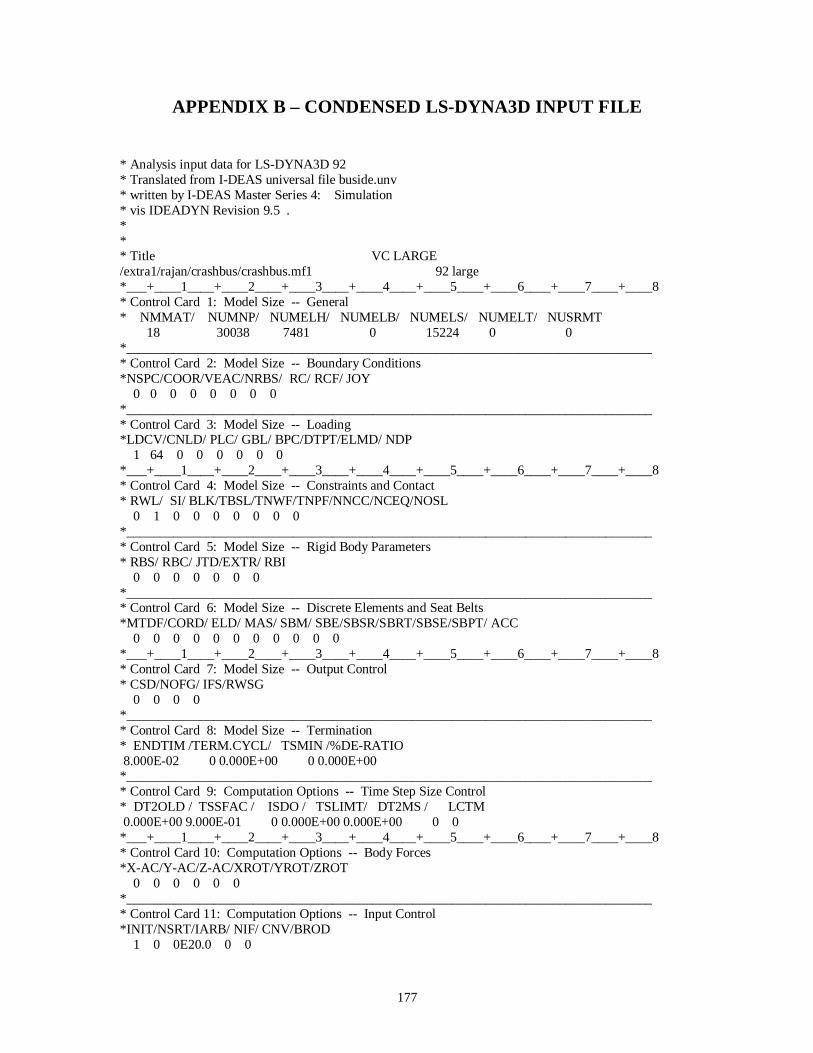
177

APPENDIX B – CONDENSED LS-DYNA3D INPUT FILE

* Analysis input data for LS-DYNA3D 92* Translated from I-DEAS universal file buside.unv* written by I-DEAS Master Series 4: Simulation* vis IDEADYN Revision 9.5 .*** Title VC LARGE/extra1/rajan/crashbus/crashbus.mf1 92 large*___+____1____+____2____+____3____+____4____+____5____+____6____+____7____+____8* Control Card 1: Model Size -- General* NMMAT/ NUMNP/ NUMELH/ NUMELB/ NUMELS/ NUMELT/ NUSRMT 18 30038 7481 0 15224 0 0*_______________________________________________________________________________* Control Card 2: Model Size -- Boundary Conditions*NSPC/COOR/VEAC/NRBS/ RC/ RCF/ JOY 0 0 0 0 0 0 0 0*_______________________________________________________________________________* Control Card 3: Model Size -- Loading*LDCV/CNLD/ PLC/ GBL/ BPC/DTPT/ELMD/ NDP 1 64 0 0 0 0 0 0*___+____1____+____2____+____3____+____4____+____5____+____6____+____7____+____8* Control Card 4: Model Size -- Constraints and Contact* RWL/ SI/ BLK/TBSL/TNWF/TNPF/NNCC/NCEQ/NOSL 0 1 0 0 0 0 0 0 0*_______________________________________________________________________________* Control Card 5: Model Size -- Rigid Body Parameters* RBS/ RBC/ JTD/EXTR/ RBI 0 0 0 0 0 0 0*_______________________________________________________________________________* Control Card 6: Model Size -- Discrete Elements and Seat Belts*MTDF/CORD/ ELD/ MAS/ SBM/ SBE/SBSR/SBRT/SBSE/SBPT/ ACC 0 0 0 0 0 0 0 0 0 0 0*___+____1____+____2____+____3____+____4____+____5____+____6____+____7____+____8* Control Card 7: Model Size -- Output Control* CSD/NOFG/ IFS/RWSG 0 0 0 0*_______________________________________________________________________________* Control Card 8: Model Size -- Termination* ENDTIM /TERM.CYCL/ TSMIN /%DE-RATIO 8.000E-02 0 0.000E+00 0 0.000E+00*_______________________________________________________________________________* Control Card 9: Computation Options -- Time Step Size Control* DT2OLD / TSSFAC / ISDO / TSLIMT/ DT2MS / LCTM 0.000E+00 9.000E-01 0 0.000E+00 0.000E+00 0 0*___+____1____+____2____+____3____+____4____+____5____+____6____+____7____+____8* Control Card 10: Computation Options -- Body Forces*X-AC/Y-AC/Z-AC/XROT/YROT/ZROT 0 0 0 0 0 0*_______________________________________________________________________________* Control Card 11: Computation Options -- Input Control*INIT/NSRT/IARB/ NIF/ CNV/BROD 1 0 0E20.0 0 0

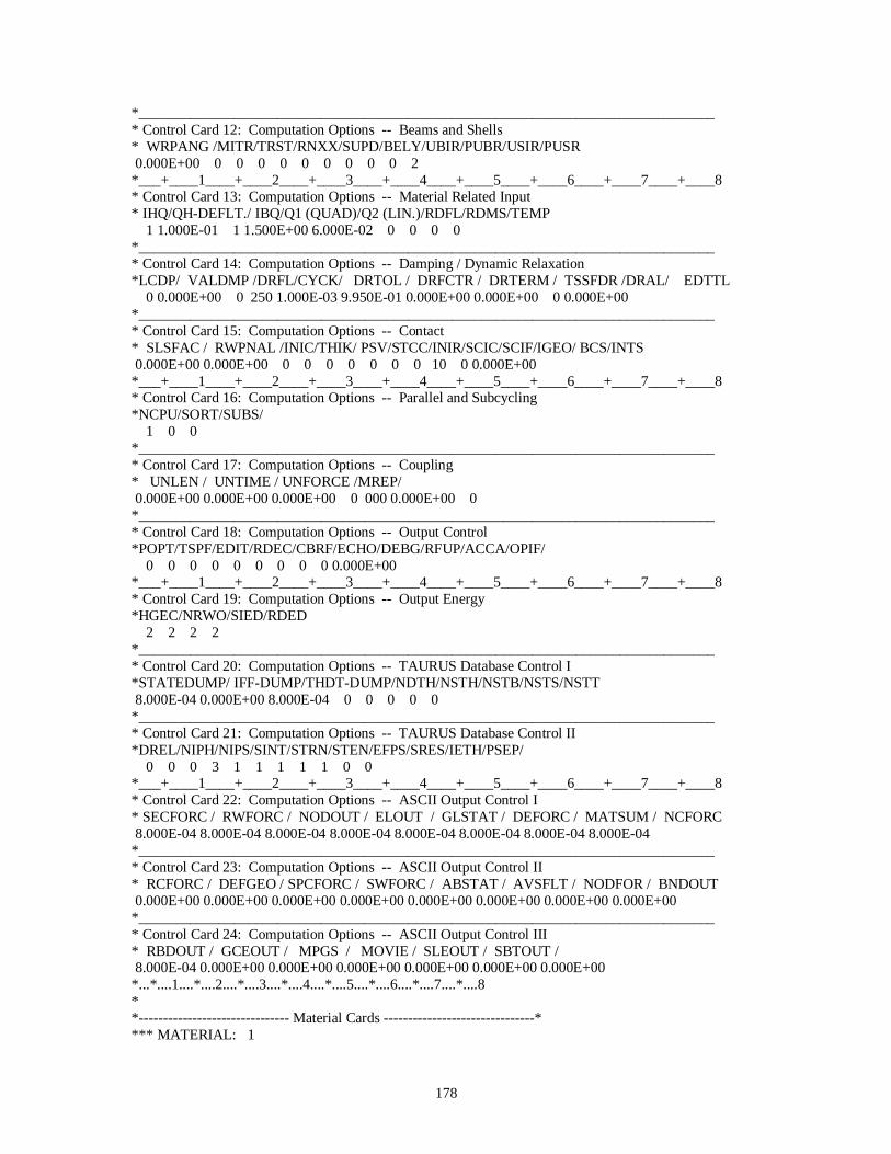
178

*_______________________________________________________________________________* Control Card 12: Computation Options -- Beams and Shells* WRPANG /MITR/TRST/RNXX/SUPD/BELY/UBIR/PUBR/USIR/PUSR 0.000E+00 0 0 0 0 0 0 0 0 0 2*___+____1____+____2____+____3____+____4____+____5____+____6____+____7____+____8* Control Card 13: Computation Options -- Material Related Input* IHQ/QH-DEFLT./ IBQ/Q1 (QUAD)/Q2 (LIN.)/RDFL/RDMS/TEMP 1 1.000E-01 1 1.500E+00 6.000E-02 0 0 0 0*_______________________________________________________________________________* Control Card 14: Computation Options -- Damping / Dynamic Relaxation*LCDP/ VALDMP /DRFL/CYCK/ DRTOL / DRFCTR / DRTERM / TSSFDR /DRAL/ EDTTL 0 0.000E+00 0 250 1.000E-03 9.950E-01 0.000E+00 0.000E+00 0 0.000E+00*_______________________________________________________________________________* Control Card 15: Computation Options -- Contact* SLSFAC / RWPNAL /INIC/THIK/ PSV/STCC/INIR/SCIC/SCIF/IGEO/ BCS/INTS 0.000E+00 0.000E+00 0 0 0 0 0 0 0 10 0 0.000E+00*___+____1____+____2____+____3____+____4____+____5____+____6____+____7____+____8* Control Card 16: Computation Options -- Parallel and Subcycling*NCPU/SORT/SUBS/ 1 0 0*_______________________________________________________________________________* Control Card 17: Computation Options -- Coupling* UNLEN / UNTIME / UNFORCE /MREP/ 0.000E+00 0.000E+00 0.000E+00 0 000 0.000E+00 0*_______________________________________________________________________________* Control Card 18: Computation Options -- Output Control*POPT/TSPF/EDIT/RDEC/CBRF/ECHO/DEBG/RFUP/ACCA/OPIF/ 0 0 0 0 0 0 0 0 0 0.000E+00*___+____1____+____2____+____3____+____4____+____5____+____6____+____7____+____8* Control Card 19: Computation Options -- Output Energy*HGEC/NRWO/SIED/RDED 2 2 2 2*_______________________________________________________________________________* Control Card 20: Computation Options -- TAURUS Database Control I*STATEDUMP/ IFF-DUMP/THDT-DUMP/NDTH/NSTH/NSTB/NSTS/NSTT 8.000E-04 0.000E+00 8.000E-04 0 0 0 0 0*_______________________________________________________________________________* Control Card 21: Computation Options -- TAURUS Database Control II*DREL/NIPH/NIPS/SINT/STRN/STEN/EFPS/SRES/IETH/PSEP/ 0 0 0 3 1 1 1 1 1 0 0*___+____1____+____2____+____3____+____4____+____5____+____6____+____7____+____8* Control Card 22: Computation Options -- ASCII Output Control I* SECFORC / RWFORC / NODOUT / ELOUT / GLSTAT / DEFORC / MATSUM / NCFORC 8.000E-04 8.000E-04 8.000E-04 8.000E-04 8.000E-04 8.000E-04 8.000E-04 8.000E-04*_______________________________________________________________________________* Control Card 23: Computation Options -- ASCII Output Control II* RCFORC / DEFGEO / SPCFORC / SWFORC / ABSTAT / AVSFLT / NODFOR / BNDOUT 0.000E+00 0.000E+00 0.000E+00 0.000E+00 0.000E+00 0.000E+00 0.000E+00 0.000E+00*_______________________________________________________________________________* Control Card 24: Computation Options -- ASCII Output Control III* RBDOUT / GCEOUT / MPGS / MOVIE / SLEOUT / SBTOUT / 8.000E-04 0.000E+00 0.000E+00 0.000E+00 0.000E+00 0.000E+00 0.000E+00*...*....1....*....2....*....3....*....4....*....5....*....6....*....7....*....8**------------------------------- Material Cards -------------------------------**** MATERIAL: 1

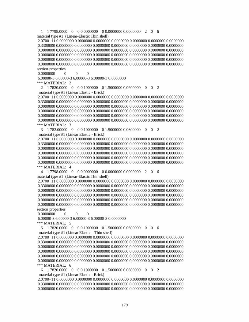
179

1 1 7798.0000 0 0 0.0000000 0 0.0000000 0.0000000 2 0 6material type #1 (Linear-Elastic Thin shell) 2.0700+11 0.0000000 0.0000000 0.0000000 0.0000000 0.0000000 0.0000000 0.0000000 0.3300000 0.0000000 0.0000000 0.0000000 0.0000000 0.0000000 0.0000000 0.0000000 0.0000000 0.0000000 0.0000000 0.0000000 0.0000000 0.0000000 0.0000000 0.0000000 0.0000000 0.0000000 0.0000000 0.0000000 0.0000000 0.0000000 0.0000000 0.0000000 0.0000000 0.0000000 0.0000000 0.0000000 0.0000000 0.0000000 0.0000000 0.0000000 0.0000000 0.0000000 0.0000000 0.0000000 0.0000000 0.0000000 0.0000000 0.0000000section properties 0.0000000 0 0 0 6.00000-3 6.00000-3 6.00000-3 6.00000-3 0.0000000*** MATERIAL: 2 2 1 7820.0000 0 0 0.1000000 0 1.5000000 0.0600000 0 0 2 material type #1 (Linear Elastic - Brick) 2.0700+11 0.0000000 0.0000000 0.0000000 0.0000000 0.0000000 0.0000000 0.0000000 0.3300000 0.0000000 0.0000000 0.0000000 0.0000000 0.0000000 0.0000000 0.0000000 0.0000000 0.0000000 0.0000000 0.0000000 0.0000000 0.0000000 0.0000000 0.0000000 0.0000000 0.0000000 0.0000000 0.0000000 0.0000000 0.0000000 0.0000000 0.0000000 0.0000000 0.0000000 0.0000000 0.0000000 0.0000000 0.0000000 0.0000000 0.0000000 0.0000000 0.0000000 0.0000000 0.0000000 0.0000000 0.0000000 0.0000000 0.0000000*** MATERIAL: 3 3 1 782.00000 0 0 0.1000000 0 1.5000000 0.0600000 0 0 2 material type #1 (Linear Elastic - Brick) 2.0700+11 0.0000000 0.0000000 0.0000000 0.0000000 0.0000000 0.0000000 0.0000000 0.3300000 0.0000000 0.0000000 0.0000000 0.0000000 0.0000000 0.0000000 0.0000000 0.0000000 0.0000000 0.0000000 0.0000000 0.0000000 0.0000000 0.0000000 0.0000000 0.0000000 0.0000000 0.0000000 0.0000000 0.0000000 0.0000000 0.0000000 0.0000000 0.0000000 0.0000000 0.0000000 0.0000000 0.0000000 0.0000000 0.0000000 0.0000000 0.0000000 0.0000000 0.0000000 0.0000000 0.0000000 0.0000000 0.0000000 0.0000000*** MATERIAL: 4 4 1 7798.0000 0 0 0.0000000 0 0.0000000 0.0000000 2 0 6material type #1 (Linear-Elastic Thin shell) 2.0700+11 0.0000000 0.0000000 0.0000000 0.0000000 0.0000000 0.0000000 0.0000000 0.3300000 0.0000000 0.0000000 0.0000000 0.0000000 0.0000000 0.0000000 0.0000000 0.0000000 0.0000000 0.0000000 0.0000000 0.0000000 0.0000000 0.0000000 0.0000000 0.0000000 0.0000000 0.0000000 0.0000000 0.0000000 0.0000000 0.0000000 0.0000000 0.0000000 0.0000000 0.0000000 0.0000000 0.0000000 0.0000000 0.0000000 0.0000000 0.0000000 0.0000000 0.0000000 0.0000000 0.0000000 0.0000000 0.0000000 0.0000000section properties 0.0000000 0 0 0 6.00000-3 6.00000-3 6.00000-3 6.00000-3 0.0000000*** MATERIAL: 5 5 1 7820.0000 0 0 0.1000000 0 1.5000000 0.0600000 0 0 6 material type #1 (Linear Elastic – Thin shell) 2.0700+11 0.0000000 0.0000000 0.0000000 0.0000000 0.0000000 0.0000000 0.0000000 0.3300000 0.0000000 0.0000000 0.0000000 0.0000000 0.0000000 0.0000000 0.0000000 0.0000000 0.0000000 0.0000000 0.0000000 0.0000000 0.0000000 0.0000000 0.0000000 0.0000000 0.0000000 0.0000000 0.0000000 0.0000000 0.0000000 0.0000000 0.0000000 0.0000000 0.0000000 0.0000000 0.0000000 0.0000000 0.0000000 0.0000000 0.0000000 0.0000000 0.0000000 0.0000000 0.0000000 0.0000000 0.0000000 0.0000000 0.0000000*** MATERIAL: 6 6 1 7820.0000 0 0 0.1000000 0 1.5000000 0.0600000 0 0 2 material type #1 (Linear Elastic - Brick) 2.0700+11 0.0000000 0.0000000 0.0000000 0.0000000 0.0000000 0.0000000 0.0000000 0.3300000 0.0000000 0.0000000 0.0000000 0.0000000 0.0000000 0.0000000 0.0000000 0.0000000 0.0000000 0.0000000 0.0000000 0.0000000 0.0000000 0.0000000 0.0000000

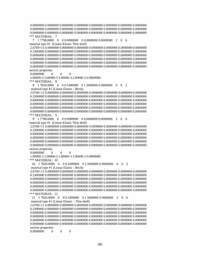
180

0.0000000 0.0000000 0.0000000 0.0000000 0.0000000 0.0000000 0.0000000 0.0000000 0.0000000 0.0000000 0.0000000 0.0000000 0.0000000 0.0000000 0.0000000 0.0000000 0.0000000 0.0000000 0.0000000 0.0000000 0.0000000 0.0000000 0.0000000 0.0000000*** MATERIAL: 7 7 1 7798.0000 0 0 0.0000000 0 0.0000000 0.0000000 2 0 6material type #1 (Linear-Elastic Thin shell) 2.0700+11 0.0000000 0.0000000 0.0000000 0.0000000 0.0000000 0.0000000 0.0000000 0.3300000 0.0000000 0.0000000 0.0000000 0.0000000 0.0000000 0.0000000 0.0000000 0.0000000 0.0000000 0.0000000 0.0000000 0.0000000 0.0000000 0.0000000 0.0000000 0.0000000 0.0000000 0.0000000 0.0000000 0.0000000 0.0000000 0.0000000 0.0000000 0.0000000 0.0000000 0.0000000 0.0000000 0.0000000 0.0000000 0.0000000 0.0000000 0.0000000 0.0000000 0.0000000 0.0000000 0.0000000 0.0000000 0.0000000 0.0000000section properties 0.0000000 0 0 0 2.00000-3 2.00000-3 2.00000-3 2.00000-3 0.0000000*** MATERIAL: 8 8 1 7820.0000 0 0 0.1000000 0 1.5000000 0.0600000 0 0 2 material type #1 (Linear Elastic - Brick) 2.0700+11 0.0000000 0.0000000 0.0000000 0.0000000 0.0000000 0.0000000 0.0000000 0.3300000 0.0000000 0.0000000 0.0000000 0.0000000 0.0000000 0.0000000 0.0000000 0.0000000 0.0000000 0.0000000 0.0000000 0.0000000 0.0000000 0.0000000 0.0000000 0.0000000 0.0000000 0.0000000 0.0000000 0.0000000 0.0000000 0.0000000 0.0000000 0.0000000 0.0000000 0.0000000 0.0000000 0.0000000 0.0000000 0.0000000 0.0000000 0.0000000 0.0000000 0.0000000 0.0000000 0.0000000 0.0000000 0.0000000 0.0000000*** MATERIAL: 9 9 1 7798.0000 0 0 0.0000000 0 0.0000000 0.0000000 2 0 6material type #1 (Linear-Elastic Thin shell) 2.0700+11 0.0000000 0.0000000 0.0000000 0.0000000 0.0000000 0.0000000 0.0000000 0.3300000 0.0000000 0.0000000 0.0000000 0.0000000 0.0000000 0.0000000 0.0000000 0.0000000 0.0000000 0.0000000 0.0000000 0.0000000 0.0000000 0.0000000 0.0000000 0.0000000 0.0000000 0.0000000 0.0000000 0.0000000 0.0000000 0.0000000 0.0000000 0.0000000 0.0000000 0.0000000 0.0000000 0.0000000 0.0000000 0.0000000 0.0000000 0.0000000 0.0000000 0.0000000 0.0000000 0.0000000 0.0000000 0.0000000 0.0000000section properties 0.0000000 0 0 0 1.00000-3 1.00000-3 1.00000-3 1.00000-3 0.0000000*** MATERIAL: 10 10 1 7820.0000 0 0 0.1000000 0 1.5000000 0.0600000 0 0 2 material type #1 (Linear Elastic - Brick) 2.0700+11 0.0000000 0.0000000 0.0000000 0.0000000 0.0000000 0.0000000 0.0000000 0.3300000 0.0000000 0.0000000 0.0000000 0.0000000 0.0000000 0.0000000 0.0000000 0.0000000 0.0000000 0.0000000 0.0000000 0.0000000 0.0000000 0.0000000 0.0000000 0.0000000 0.0000000 0.0000000 0.0000000 0.0000000 0.0000000 0.0000000 0.0000000 0.0000000 0.0000000 0.0000000 0.0000000 0.0000000 0.0000000 0.0000000 0.0000000 0.0000000 0.0000000 0.0000000 0.0000000 0.0000000 0.0000000 0.0000000 0.0000000*** MATERIAL: 11 11 1 7820.0000 0 0 0.1000000 0 1.5000000 0.0600000 2 0 6 material type #1 (Linear Elastic – Thin shell) 2.0700+11 0.0000000 0.0000000 0.0000000 0.0000000 0.0000000 0.0000000 0.0000000 0.3300000 0.0000000 0.0000000 0.0000000 0.0000000 0.0000000 0.0000000 0.0000000 0.0000000 0.0000000 0.0000000 0.0000000 0.0000000 0.0000000 0.0000000 0.0000000 0.0000000 0.0000000 0.0000000 0.0000000 0.0000000 0.0000000 0.0000000 0.0000000 0.0000000 0.0000000 0.0000000 0.0000000 0.0000000 0.0000000 0.0000000 0.0000000 0.0000000 0.0000000 0.0000000 0.0000000 0.0000000 0.0000000 0.0000000 0.0000000 section properties 0.0000000 0 0 0

181

1.00000-3 1.00000-3 1.00000-3 1.00000-3 0.0000000*** MATERIAL: 12 12 1 7820.0000 0 0 0.1000000 0 1.5000000 0.0600000 0 0 2 material type #1 (Linear Elastic - Brick) 2.0700+11 0.0000000 0.0000000 0.0000000 0.0000000 0.0000000 0.0000000 0.0000000 0.3300000 0.0000000 0.0000000 0.0000000 0.0000000 0.0000000 0.0000000 0.0000000 0.0000000 0.0000000 0.0000000 0.0000000 0.0000000 0.0000000 0.0000000 0.0000000 0.0000000 0.0000000 0.0000000 0.0000000 0.0000000 0.0000000 0.0000000 0.0000000 0.0000000 0.0000000 0.0000000 0.0000000 0.0000000 0.0000000 0.0000000 0.0000000 0.0000000 0.0000000 0.0000000 0.0000000 0.0000000 0.0000000 0.0000000 0.0000000*** MATERIAL: 13 13 1 7820.0000 0 0 0.1000000 0 1.5000000 0.0600000 0 0 2 material type #1 (Linear Elastic – Brick) 2.0700+11 0.0000000 0.0000000 0.0000000 0.0000000 0.0000000 0.0000000 0.0000000 0.3300000 0.0000000 0.0000000 0.0000000 0.0000000 0.0000000 0.0000000 0.0000000 0.0000000 0.0000000 0.0000000 0.0000000 0.0000000 0.0000000 0.0000000 0.0000000 0.0000000 0.0000000 0.0000000 0.0000000 0.0000000 0.0000000 0.0000000 0.0000000 0.0000000 0.0000000 0.0000000 0.0000000 0.0000000 0.0000000 0.0000000 0.0000000 0.0000000 0.0000000 0.0000000 0.0000000 0.0000000 0.0000000 0.0000000 0.0000000*** MATERIAL: 14 14 1 7798.0000 0 0 0.0000000 0 0.0000000 0.0000000 2 0 6material type #1 (Linear-Elastic Thin shell) 2.0700+11 0.0000000 0.0000000 0.0000000 0.0000000 0.0000000 0.0000000 0.0000000 0.3300000 0.0000000 0.0000000 0.0000000 0.0000000 0.0000000 0.0000000 0.0000000 0.0000000 0.0000000 0.0000000 0.0000000 0.0000000 0.0000000 0.0000000 0.0000000 0.0000000 0.0000000 0.0000000 0.0000000 0.0000000 0.0000000 0.0000000 0.0000000 0.0000000 0.0000000 0.0000000 0.0000000 0.0000000 0.0000000 0.0000000 0.0000000 0.0000000 0.0000000 0.0000000 0.0000000 0.0000000 0.0000000 0.0000000 0.0000000section properties 0.0000000 0 0 0 2.00000-3 2.00000-3 2.00000-3 2.00000-3 0.0000000*** MATERIAL: 15 15 1 7820.0000 0 0 0.1000000 0 1.5000000 0.0600000 0 0 2 material type #1 (Linear Elastic - Brick) 2.0700+11 0.0000000 0.0000000 0.0000000 0.0000000 0.0000000 0.0000000 0.0000000 0.3300000 0.0000000 0.0000000 0.0000000 0.0000000 0.0000000 0.0000000 0.0000000 0.0000000 0.0000000 0.0000000 0.0000000 0.0000000 0.0000000 0.0000000 0.0000000 0.0000000 0.0000000 0.0000000 0.0000000 0.0000000 0.0000000 0.0000000 0.0000000 0.0000000 0.0000000 0.0000000 0.0000000 0.0000000 0.0000000 0.0000000 0.0000000 0.0000000 0.0000000 0.0000000 0.0000000 0.0000000 0.0000000 0.0000000 0.0000000*** MATERIAL: 16 16 1 7798.0000 0 0 0.0000000 0 0.0000000 0.0000000 2 0 6material type #1 (Linear-Elastic Thin shell) 2.0700+11 0.0000000 0.0000000 0.0000000 0.0000000 0.0000000 0.0000000 0.0000000 0.3300000 0.0000000 0.0000000 0.0000000 0.0000000 0.0000000 0.0000000 0.0000000 0.0000000 0.0000000 0.0000000 0.0000000 0.0000000 0.0000000 0.0000000 0.0000000 0.0000000 0.0000000 0.0000000 0.0000000 0.0000000 0.0000000 0.0000000 0.0000000 0.0000000 0.0000000 0.0000000 0.0000000 0.0000000 0.0000000 0.0000000 0.0000000 0.0000000 0.0000000 0.0000000 0.0000000 0.0000000 0.0000000 0.0000000 0.0000000 section properties 0.0000000 0 0 0 6.00000-3 6.00000-3 6.00000-3 6.00000-3 0.0000000*** MATERIAL: 17 17 1 7798.0000 0 0 0.0000000 0 0.0000000 0.0000000 2 0 6material type #1 (Linear-Elastic Thin shell) 2.0700+11 0.0000000 0.0000000 0.0000000 0.0000000 0.0000000 0.0000000 0.0000000

182

0.3300000 0.0000000 0.0000000 0.0000000 0.0000000 0.0000000 0.0000000 0.0000000 0.0000000 0.0000000 0.0000000 0.0000000 0.0000000 0.0000000 0.0000000 0.0000000 0.0000000 0.0000000 0.0000000 0.0000000 0.0000000 0.0000000 0.0000000 0.0000000 0.0000000 0.0000000 0.0000000 0.0000000 0.0000000 0.0000000 0.0000000 0.0000000 0.0000000 0.0000000 0.0000000 0.0000000 0.0000000 0.0000000 0.0000000 0.0000000 section properties 0.0000000 0 0 0 2.00000-3 2.00000-3 2.00000-3 2.00000-3 0.0000000*** MATERIAL: 18 18 1 7798.0000 0 0 0.0000000 0 0.0000000 0.0000000 0 0 2material type #1 (Linear-Elastic Brick) 2.0700+11 0.0000000 0.0000000 0.0000000 0.0000000 0.0000000 0.0000000 0.0000000 0.3300000 0.0000000 0.0000000 0.0000000 0.0000000 0.0000000 0.0000000 0.0000000 0.0000000 0.0000000 0.0000000 0.0000000 0.0000000 0.0000000 0.0000000 0.0000000 0.0000000 0.0000000 0.0000000 0.0000000 0.0000000 0.0000000 0.0000000 0.0000000 0.0000000 0.0000000 0.0000000 0.0000000 0.0000000 0.0000000 0.0000000 0.0000000 0.0000000 0.0000000 0.0000000 0.0000000 0.0000000 0.0000000 0.0000000 0.0000000**...*....1....*....2....*....3....*....4....*....5....*....6....*....7....*....8**------------------------------ Node Definitions ------------------------------** #/ DBC/ X-COOR / Y-COOR / Z-COOR / RBC 1 0 0.0000000000000E+00 6.1199998855591E-01 0.0000000000000E+00 0 2 0-1.5727986226699E-15 7.2109442949295E-01-1.5748000144958E+00 0 3 0-2.7755575615629E-17 3.9098110795021E-01 0.0000000000000E+00 0 4 0-2.2204460492503E-16-2.2859999537468E-01 0.0000000000000E+00 0 5 0-1.7157831575317E-16-3.7548467516899E-02 0.0000000000000E+00 0 6 0 1.6653345369377E-16 1.0989576578140E-01 0.0000000000000E+00 0 7 0-1.0320502215742E-16 2.2129407525063E-01 0.0000000000000E+00 0 8 0 2.4980018054066E-16 2.7645480632782E-01 0.0000000000000E+00 0 9 0-1.4720162073859E-16 5.4735042154789E-02 0.0000000000000E+00 0 10 0-1.5727986226699E-15 4.2102333903313E-01-1.5748000144958E+00 0...... 30027 0 1.2491999864578E+00 7.6956778764725E-01-4.6461100578308E+00 0 30028 0 1.2491999864578E+00 7.6956778764725E-01-4.7611112594604E+00 0 30029 0 1.2491999864578E+00 7.6956778764725E-01-4.8761100769043E+00 0 30030 0 1.2491999864578E+00 7.6956778764725E-01-4.9911112785339E+00 0 30031 0 1.2491999864578E+00 7.6956778764725E-01-5.1061100959778E+00 0 30032 0 1.2491999864578E+00 7.6956778764725E-01-5.2211112976074E+00 0 30033 0 1.2491999864578E+00 7.6956778764725E-01-5.3361101150513E+00 0 30034 0 1.2491999864578E+00 7.6956778764725E-01-5.4511079788208E+00 0 30035 0 1.2491999864578E+00 7.6956778764725E-01-5.5661101341248E+00 0 30036 0 1.2491999864578E+00 7.6956778764725E-01-5.6811113357544E+00 0 30037 0 1.2491999864578E+00 7.6956778764725E-01-5.7961077690125E+00 0 30038 0 1.2491999864578E+00 7.6956778764725E-01-5.9111080169678E+00 0*...*....1....*....2....*....3....*....4....*....5....*....6....*....7....*....8**---------------------- Element Cards for Solid Elements ----------------------** #/ MAT/ N1/ N2/ N3/ N4/ N5/ N6/ N7/ N8/ 1 12 1063 1062 1064 1065 1383 1382 1384 1385 2 12 1073 1072 1074 1075 1393 1392 1394 1395

183

3 12 1075 1074 1076 1077 1395 1394 1396 1397 4 12 1077 1076 1078 1079 1397 1396 1398 1399 5 12 1079 1078 1080 1081 1399 1398 1400 1401 6 12 1081 1080 1082 1083 1401 1400 1402 1403 7 12 1083 1082 1084 1085 1403 1402 1404 1405 8 12 1085 1084 1086 1087 1405 1404 1406 1407 9 12 1089 1088 1090 1091 1409 1408 1410 1411 10 12 1091 1090 1092 1093 1411 1410 1412 1413...... 7471 19 29707 30007 30027 29727 29708 30008 30028 29728 7472 19 29708 30008 30028 29728 29709 30009 30029 29729 7473 19 29709 30009 30029 29729 29710 30010 30030 29730 7474 19 29710 30010 30030 29730 29711 30011 30031 29731 7475 19 29711 30011 30031 29731 29712 30012 30032 29732 7476 19 29712 30012 30032 29732 29713 30013 30033 29733 7477 19 29713 30013 30033 29733 29714 30014 30034 29734 7478 19 29714 30014 30034 29734 29715 30015 30035 29735 7479 19 29715 30015 30035 29735 29716 30016 30036 29736 7480 19 29716 30016 30036 29736 29717 30017 30037 29737 7481 19 29717 30017 30037 29737 29718 30018 30038 29738*...*....1....*....2....*....3....*....4....*....5....*....6....*....7....*....8**------------------- Element Cards for Thin Shell Elements -------------------** #/ MAT/ N1/ N2/ N3/ N4/ 1 17 474 632 471 439 9.000E-04 9.000E-04 9.000E-04 9.000E-04 2 17 475 631 632 474 9.000E-04 9.000E-04 9.000E-04 9.000E-04 3 17 633 472 438 470 9.000E-04 9.000E-04 9.000E-04 9.000E-04 4 17 631 472 633 632 9.000E-04 9.000E-04 9.000E-04 9.000E-04 5 17 632 633 470 471 9.000E-04 9.000E-04 9.000E-04 9.000E-04 6 17 473 440 472 631 9.000E-04 9.000E-04 9.000E-04 9.000E-04 7 17 441 473 631 475 9.000E-04 9.000E-04 9.000E-04 9.000E-04 8 17 635 477 478 634 9.000E-04 9.000E-04 9.000E-04 9.000E-04 9 17 481 635 634 480 9.000E-04 9.000E-04 9.000E-04 9.000E-04 10 17 440 476 636 438 9.000E-04 9.000E-04 9.000E-04 9.000E-04......

184

15211 1 27228 27571 27572 26089 6.000E-03 6.000E-03 6.000E-03 6.000E-03 15212 1 27226 27571 27572 25438 6.000E-03 6.000E-03 6.000E-03 6.000E-03 15213 1 27225 27571 27572 26087 6.000E-03 6.000E-03 6.000E-03 6.000E-03 15214 1 27224 27571 27572 26087 6.000E-03 6.000E-03 6.000E-03 6.000E-03 15215 1 27223 27571 27572 25437 6.000E-03 6.000E-03 6.000E-03 6.000E-03 15216 1 27222 27571 27572 25437 6.000E-03 6.000E-03 6.000E-03 6.000E-03 15217 1 27571 27220 26085 27572 6.000E-03 6.000E-03 6.000E-03 6.000E-03 15218 1 27571 27219 26084 27572 6.000E-03 6.000E-03 6.000E-03 6.000E-03 15219 1 27571 27218 25444 27572 6.000E-03 6.000E-03 6.000E-03 6.000E-03 15220 1 27571 27217 26083 27572 6.000E-03 6.000E-03 6.000E-03 6.000E-03 15221 1 27571 27215 25445 27572 6.000E-03 6.000E-03 6.000E-03 6.000E-03 15222 1 27571 27214 26082 27572 6.000E-03 6.000E-03 6.000E-03 6.000E-03 15223 1 27571 27213 25439 27572 6.000E-03 6.000E-03 6.000E-03 6.000E-03 15224 1 27571 26077 26081 27572 6.000E-03 6.000E-03 6.000E-03 6.000E-03*----------------------- LOAD CURVE DEFINITIONS -----------------------* 1 3 0 1.0000000 1.0000000 0.0000000 0.0000000 0.0000000-246.00000 0.5000000-246.00000 1.0000000-246.00000* NODAL LOAD DEFINITIONS ******...*....1....*....2....*....3....*....4....*....5....*....6....*....7....*....8 27592 2 1 1 0 0 0 0 0 27593 2 1 1 0 0 0 0 0 27594 2 1 1 0 0 0 0 0 27595 2 1 1 0 0 0 0 0 27596 2 1 1 0 0 0 0 0 27597 2 1 1 0 0 0 0 0 27598 2 1 1 0 0 0 0 0 27599 2 1 1 0 0 0 0 0 27600 2 1 1 0 0 0 0 0 27601 2 1 1 0 0 0 0 0 27602 2 1 1 0 0 0 0 0 27603 2 1 1 0 0 0 0 0 27604 2 1 1 0 0 0 0 0 27605 2 1 1 0 0 0 0 0 27606 2 1 1 0 0 0 0 0 27607 2 1 1 0 0 0 0 0 27608 2 1 1 0 0 0 0 0 27609 2 1 1 0 0 0 0 0 27610 2 1 1 0 0 0 0 0 27611 2 1 1 0 0 0 0 0 27612 2 1 1 0 0 0 0 0

185

27613 2 1 1 0 0 0 0 0 27614 2 1 1 0 0 0 0 0 27615 2 1 1 0 0 0 0 0 27616 2 1 1 0 0 0 0 0 27617 2 1 1 0 0 0 0 0 27618 2 1 1 0 0 0 0 0 27619 2 1 1 0 0 0 0 0 27620 2 1 1 0 0 0 0 0 27621 2 1 1 0 0 0 0 0 27622 2 1 1 0 0 0 0 0 27623 2 1 1 0 0 0 0 0 27689 2 1 1 0 0 0 0 0 27690 2 1 1 0 0 0 0 0 27691 2 1 1 0 0 0 0 0 27692 2 1 1 0 0 0 0 0 27717 2 1 1 0 0 0 0 0 27718 2 1 1 0 0 0 0 0 27719 2 1 1 0 0 0 0 0 27720 2 1 1 0 0 0 0 0 27721 2 1 1 0 0 0 0 0 27722 2 1 1 0 0 0 0 0 27723 2 1 1 0 0 0 0 0 27724 2 1 1 0 0 0 0 0 27725 2 1 1 0 0 0 0 0 27726 2 1 1 0 0 0 0 0 27727 2 1 1 0 0 0 0 0 27728 2 1 1 0 0 0 0 0 27757 2 1 1 0 0 0 0 0 27758 2 1 1 0 0 0 0 0 27759 2 1 1 0 0 0 0 0 27760 2 1 1 0 0 0 0 0 27761 2 1 1 0 0 0 0 0 27762 2 1 1 0 0 0 0 0 27763 2 1 1 0 0 0 0 0 27764 2 1 1 0 0 0 0 0 27765 2 1 1 0 0 0 0 0 27766 2 1 1 0 0 0 0 0 27767 2 1 1 0 0 0 0 0 27768 2 1 1 0 0 0 0 0 27769 2 1 1 0 0 0 0 0 27770 2 1 1 0 0 0 0 0 27771 2 1 1 0 0 0 0 0 27772 2 1 1 0 0 0 0 0*...*....1....*....2....*....3....*....4....*....5....*....6....*....7....*....8**----------------------------- Initial Conditions -----------------------------** #/ IVX/ IVY/ IVZ 1 0.000E+00 0.000E+00 0.000E+00 2 0.000E+00 0.000E+00 0.000E+00 3 0.000E+00 0.000E+00 0.000E+00 4 0.000E+00 0.000E+00 0.000E+00 5 0.000E+00 0.000E+00 0.000E+00 6 0.000E+00 0.000E+00 0.000E+00 7 0.000E+00 0.000E+00 0.000E+00 8 0.000E+00 0.000E+00 0.000E+00 9 0.000E+00 0.000E+00 0.000E+00

186

10 0.000E+00 0.000E+00 0.000E+00........ 30027-1.555E+01 0.000E+00 0.000E+00 30028-1.555E+01 0.000E+00 0.000E+00 30029-1.555E+01 0.000E+00 0.000E+00 30030-1.555E+01 0.000E+00 0.000E+00 30031-1.555E+01 0.000E+00 0.000E+00 30032-1.555E+01 0.000E+00 0.000E+00 30033-1.555E+01 0.000E+00 0.000E+00 30034-1.555E+01 0.000E+00 0.000E+00 30035-1.555E+01 0.000E+00 0.000E+00 30036-1.555E+01 0.000E+00 0.000E+00 30037-1.555E+01 0.000E+00 0.000E+00 30038-1.555E+01 0.000E+00 0.000E+00*...*....1....*....2....*....3....*....4....*....5....*....6....*....7....*....8**----------------------- Sliding Interface Definitions -----------------------** NUMS/ NUMM/R//T/ NUS/ NUK/ DECC/LCN// SS/ MS/ SFSPS/ SFMPS 648 280 5 0.000E+00 0.000E+00 0.000E+00 00 1 11.0E+001.0E+00 1 8481 0 0 0 2 8482 0 0 0 3 8483 0 0 0 4 8484 0 0 0 5 8485 0 0 0 6 8486 0 0 0 7 8487 0 0 0 8 8491 0 0 0 9 8492 0 0 0 10 8493 0 0 0....... 638 13125 0 0 0 639 13126 0 0 0 640 13127 0 0 0 641 13128 0 0 0 642 13129 0 0 0 643 13130 0 0 0 644 13131 0 0 0 645 13132 0 0 0 646 13133 0 0 0 647 13134 0 0 0 648 13135 0 0 0 1 29766 29786 29787 29767 2 29739 29759 29760 29740

187

3 29740 29760 29761 29741 4 29741 29761 29762 29742 5 29742 29762 29763 29743 6 29743 29763 29764 29744 7 29744 29764 29765 29745 8 29745 29765 29766 29746 9 29746 29766 29767 29747 10 29747 29767 29768 29748....... 271 30008 30028 30029 30009 272 30009 30029 30030 30010 273 30010 30030 30031 30011 274 30011 30031 30032 30012 275 30012 30032 30033 30013 276 30013 30033 30034 30014 277 30014 30034 30035 30015 278 30015 30035 30036 30016 279 30016 30036 30037 30017 280 30017 30037 30038 30018

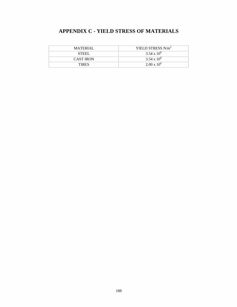
188

APPENDIX C - YIELD STRESS OF MATERIALS

MATERIAL YIELD STRESS N/m2

STEEL 3.54 x 108

CAST IRON 3.54 x 108

TIRES 2.00 x 106

189

VITA

The author Ganesh Panneer was born in Trichy, TamilNadu, India on December 9,

1973. After graduating from a high school in Trichy, he entered the Government College

of Technology and received his Bachelor of Engineering degree in Mechanical

Engineering in May 1995.

After graduating from Government College of Technology, he was working as a

Senior Development Engineer in the CAE department for Ashok Leyland Ltd., one of the

leading manufacturers of trucks and buses in India. He came to West Virginia University

for the spring semester 1997 for his graduate studies in Mechanical Engineering. This

thesis was written in May 1998 , as a partial fulfillment towards a degree in the Master of

Science in Mechanical Engineering (M.S.M.E) at the West Virginia University.

190

APPROVAL OF EXAMINING COMMITTEE

Victor H. Mucino, Ph.D.

James E. Smith, Ph.D.

Date Gregory J. Thompson, Ph.D.

Chairman

Documents

School bus crashworthiness - CORE