Scaling of Differentiation in Networks: Nervous Systems ...pdodds/teaching/courses/2009-08UVM... · the networks for which human ingenuity is involved (electronic circuits, Legos,

J. theor. Biol. (2002) 218, 215–237doi:10.1006/yjtbi.3070, available online at http://www.idealibrary.com on

Scaling of Differentiation in Networks: Nervous Systems, Organisms,Ant Colonies, Ecosystems, Businesses, Universities, Cities,

Electronic Circuits, and Legos

M. A. Changizinw, M. A. McDannaldw and D.Widdersw

wDepartment of Psychological and Brain Sciences, Duke University, Durham, NC 27708-0086, U.S.A.

(Received on 10 September 2001, Accepted in revised form on 25 April 2002)

Nodes in networks are often of different types, and in this sense networks are differentiated.Here we examine the relationship between network differentiation and network size innetworks under economic or natural selective pressure, such as electronic circuits (networksof electronic components), Legost (networks of Legot pieces), businesses (networks ofemployees), universities (networks of faculty), organisms (networks of cells), ant colonies(networks of ants), and nervous systems (networks of neurons). For each of these we find that(i) differentiation increases with network size, and (ii) the relationship is consistent with apower law. These results are explained by a hypothesis that, because nodes are costly to buildand maintain in such ‘‘selected networks’’, network size is optimized, and from this thepower-law relationship may be derived. The scaling exponent depends on the particular kindof network, and is determined by the degree to which nodes are used in a combinatorialfashion to carry out network-level functions. We find that networks under natural selection(organisms, ant colonies, and nervous systems) have much higher combinatorial abilities thanthe networks for which human ingenuity is involved (electronic circuits, Legos, businesses,and universities). A distinct but related optimization hypothesis may be used to explainscaling of differentiation in competitive networks (networks where the nodes themselves,rather than the entire network, are under selective pressure) such as ecosystems (networks oforganisms).

r 2002 Elsevier Science Ltd. All rights reserved.

1. Introduction

While there is a considerable literature studyingthe scaling properties of network connectivity[e.g. see the literature springing from the papersby Watts & Strogatz (1997) and Barab!asi &Albert (1999), and also Changizi (2001a)], there

has been comparably little attention given to oneof the most important features of networks: thatnodes within networks come in different types.Our main purpose is to examine the relationshipbetween network differentiation (i.e. the numberof node types) and network size (i.e. the totalnumber of nodes) among those kinds of networkthat are under selective pressure, whether it beeconomic or natural selection. We call suchnetworks selected networks. Consider two gen-eral relationships one might a priori expect.The first is that there is a finite set of node

nCorresponding author’s current address: Sloan-SwartzCenter for Theoretical Neurobiology, California Instituteof Technology, Pasadena, CA 91125, USA. Tel.: +1-919-660-5641; fax: +1-916-660-5726.E-mail address: [email protected] (M.A. Changizi).

0022-5193/02/$35.00/0 r 2002 Elsevier Science Ltd. All rights reserved.

typesFa universal languageFfrom which anynetwork of that kind may be built, and thusdifferentiation does not increase as a function ofnetwork size. For example, every digital circuit,no matter its size or function, can be constructedfrom just two types of node (an AND gate anda NOT gate). Thus, differentiation need notincrease as a function of network size for digitalcircuits. The second possible relationship is thatthere is no universal language, and, instead,larger networks tend to have more node types.As we will see below, it is this latter possibilitywhich appears to hold for a wide variety ofselected networks.

2. Hypothesis and Mathematical Preliminaries

In this section, we present a hypothesisconcerning the relationship between differentia-tion and size in selected networks, and alsointroduce mathematical tools for understandingthe scaling relationships.

2.1. THE INEQUALITY RELATING

COMPLEXITY E AND SIZE N

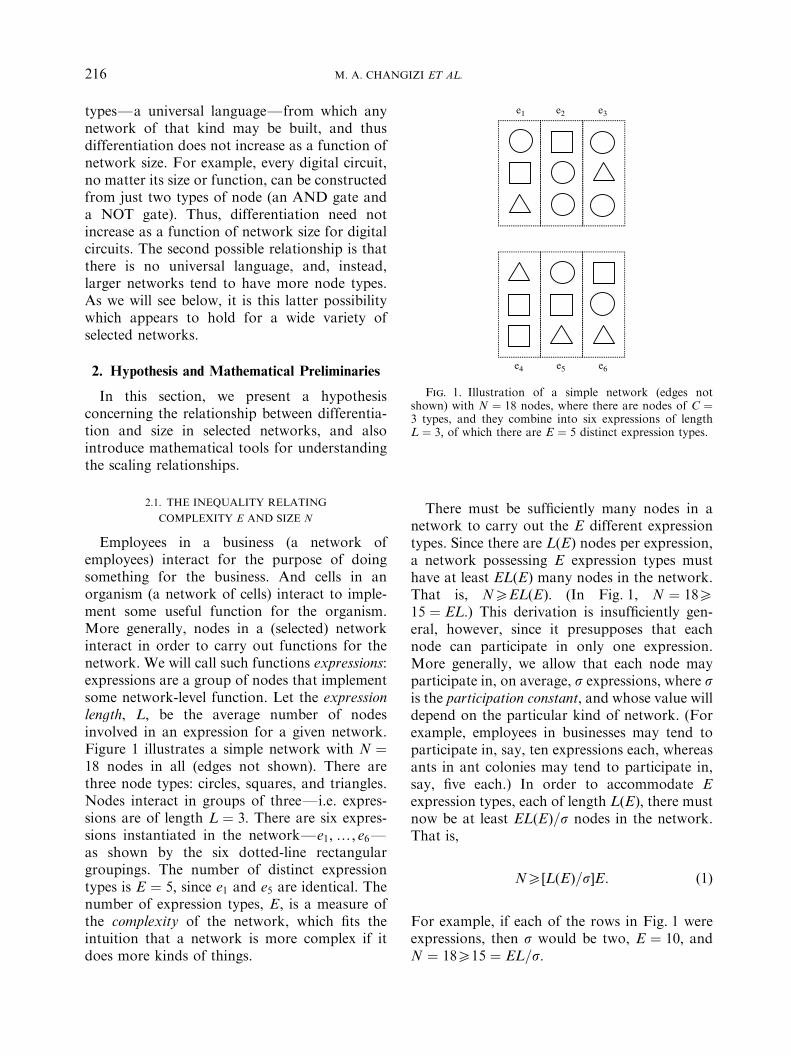
Employees in a business (a network ofemployees) interact for the purpose of doingsomething for the business. And cells in anorganism (a network of cells) interact to imple-ment some useful function for the organism.More generally, nodes in a (selected) networkinteract in order to carry out functions for thenetwork. We will call such functions expressions:expressions are a group of nodes that implementsome network-level function. Let the expressionlength, L; be the average number of nodesinvolved in an expression for a given network.Figure 1 illustrates a simple network with N !18 nodes in all (edges not shown). There arethree node types: circles, squares, and triangles.Nodes interact in groups of threeFi.e. expres-sions are of length L ! 3: There are six expres-sions instantiated in the networkFe1;y; e6Fas shown by the six dotted-line rectangulargroupings. The number of distinct expressiontypes is E ! 5; since e1 and e5 are identical. Thenumber of expression types, E; is a measure ofthe complexity of the network, which fits theintuition that a network is more complex if itdoes more kinds of things.

There must be sufficiently many nodes in anetwork to carry out the E different expressiontypes. Since there are L"E# nodes per expression,a network possessing E expression types musthave at least EL"E# many nodes in the network.That is, NXEL"E#: (In Fig. 1, N ! 18X15 ! EL:) This derivation is insufficiently gen-eral, however, since it presupposes that eachnode can participate in only one expression.More generally, we allow that each node mayparticipate in, on average, s expressions, where sis the participation constant, and whose value willdepend on the particular kind of network. (Forexample, employees in businesses may tend toparticipate in, say, ten expressions each, whereasants in ant colonies may tend to participate in,say, five each.) In order to accommodate Eexpression types, each of length L"E#; there mustnow be at least EL"E#=s nodes in the network.That is,

NX$L"E#=s%E: "1#

For example, if each of the rows in Fig. 1 wereexpressions, then s would be two, E ! 10; andN ! 18X15 ! EL=s:

e1 e2 e3

e4 e5 e6

Fig. 1. Illustration of a simple network (edges notshown) with N ! 18 nodes, where there are nodes of C !3 types, and they combine into six expressions of lengthL ! 3; of which there are E ! 5 distinct expression types.

M. A. CHANGIZI ET AL.216

2.2. THE OPTIMALITY HYPOTHESIS: RELATING

COMPLEXITY E AND SIZE N

We hypothesize that for selected networks, thefollowing Minimal N Hypothesis applies: Net-work size N does not scale up more quickly thanneeded to obtain the E expression types. Equiva-lently, the hypothesis is that network size N isminimized (or that E is maximized), up to aconstant factor. The motivation behind this isthat nodes in a selected network are costly,requiring energy of some kind to build andmaintain. [For other applications of volumeoptimization, see Cherniak et al. (1999), Chan-gizi & Cherniak (2000), and Changizi (2001a, d,in press)]. It follows that NBL"E#E: Further-more, to minimize N; L"E# must remaininvariant, for if L"E# increases with E; then Nscales up faster than needed to obtain the Eexpression types. Thus, we may derive from thishypothesis that

L is invariant; andNBE: "2#

If networks do conform to the Minimal NHypothesis, then, within any given kind ofnetwork, network size N may be used as a proxyfor network complexity E:Note that we do not generally expect the

Minimal N Hypothesis to apply to non-selectednetworks. For example, a crystalline structure isa network: the number of atoms is the networksize, and different expression types are thedifferent kinds of interacting groups of atoms.Crystalline structures are not, however, underany selective pressure, and there is nothingpreventing N from increasing (i.e. a biggercrystal) without any increase in the number ofexpression types (i.e. no increase in networkcomplexity). The Minimal N Hypothesis there-fore does not apply to crystals. Another kind ofnon-selected network is competitive networks,which are networks where there is selectivepressure on the nodes themselves, not thenetwork. Examples are ecosystems (networks oforganisms) and cities (networks of businesses).Although the Minimal N Hypothesis is notplausible for competitive networks, there aresometimes other hypotheses that do plausiblyapply and that serve as a replacement assump-tion allowing the derivation of eqn (2). We will

discuss this in subsection 3.7 when we take upecosystems.

2.3. THE RELATIONSHIP BETWEEN COMPLEXITY

E AND DIFFERENTIATION C

From the above hypothesis, we may derive theexpected relationship between network differen-tiation and size. As a step toward this, considerhow network complexity, E; relates to thenumber of node types, or differentiation, C:(Some of these notions emanate from Changizi,2001b; see also Changizi, 2001c, in press.) With Cnode types, how many length-L expression types,E; are possible? The answer is E ! C"E#L"E#: Forexample, if there are C ! 2 node typesFlabeledA and BFand expression length L ! 4; thenthere are E ! 24 ! 16 expression types, namelyAAAA, AAAB, AABA,y, BBBB. However, thisis insufficiently general for two reasons. First,only some constant fraction a of these expressiontypes will generally be grammatical, or allowable,in the network, where this proportionality con-stant will depend on the particular kind ofnetwork. The relationship is, then, EBC"E#L"E#:Second, the exponent, L; assumes that all Ldegrees of freedom in the construction of expres-sions are available, when only some fixed fractionb of the L degrees of freedom may generally beavailable due to inter-nodal constraints. Letd"E# ! bL"E#: Call this variable d the combina-torial degree. The relationship is, then,

EBC"E#d"E#: "3#

Let us use the same example above, but supposenow that A’s always occur in pairs, and that B’salso always occur in pairs. The ‘‘effectivecomponents’’ in the construction of expressionsare now just AA and BB, and the expressiontypes are AAAA, AABB, BBAA, and BBBB.The number of degrees of freedom for anexpression is just 2, not 4, and thus E ! 22 !4: Via the Minimal N Hypothesis, expressionlength, L; was invariant, and thus so is thecombinatorial degree, d: It follows that

EBC"E#d ; where d is invariant andX1: "4#

It is important to understand the meaning of‘‘combinatorial degree’’, for it will be much

SCALING OF DIFFERENTIATION IN NETWORKS 217

discussed later. It is best interpreted as, intui-tively, the ‘‘effective length of an averageexpression’’, or, ‘‘how combinatorial the expres-sions are’’, or ‘‘the number of degrees of freedomin an expression.’’ The lowest possible combina-torial degree is d ! 1; and this means that thereis effectively just one node per expression. This,in turn, means that nodes are not used in acombinatorial fashion to build expressions (de-spite the fact that L might be greater than one).A combinatorial degree greater than one meansthat nodes are used in a combinatorial fashion toconstruct expressions, and greater values meanthat expressions are more combinatorial, or‘‘effectively longer’’. [The combinatorial degreeis related to the Shannon–Boltzmann entropy Has follows: H ! &Spi log2"pi#; where i rangesfrom 1 to the number of expression types E;and pi is the probability of expression type ioccurring (Ash, 1965). Assuming that theprobabilities are uniform, p ! 1=E; and thusH ! &E$"1=E#log2"1=E#%; or H ! log2 E: Recallthat EBCd"E#; and so d ! "log2 E#="log2 C"E##;and thus it follows that d ! H"E#=log2 C"E#:That is, the combinatorial degree d is a measureof the entropy, but relative to a (possiblyincreasing) symbol set size C:]

2.4. THE RELATIONSHIP BETWEEN DIFFERENTIATION

C AND SIZE N

At this point, we have related network size Nand network (expressive) complexity E via eqn(2), and we have related E to differentiation Cvia eqn (4). Combining these equations we mayderive

NBCd ; where d is invariant andX1: "5#

That is, we have derived from the Minimal NHypothesis that we expect network size, N; torelate to network differentiation, C; as a powerlaw with exponent dX1: We will see in Section 3that this appears to be the case for selectednetworks. For each kind of network, wecompute the inverse of the best-fit slope of Cvs. N on a log–log plot, for this provides anestimate of the combinatorial degree, d: In thisway, (i) we acquire a measure of how combina-torial that kind of network is, and (ii) thecombinatorial degree provides us with a clue as

to what the expressions might be in that kind ofnetwork. [Note that eqn (5) implies thatCBN1=d ; and thus that the number of compo-nents of any given type will scale asN=CBN="N1=d # ! N1&1=d : In non-combinator-ial organizations where d ! 1; the number ofcomponents of any given type is invariant;whereas as d gets large, N=C approachesproportionality with N:]

2.5. TYPE-NETWORKS

As just discussed, plots of differentiation C vs.size N provide us with interesting informationabout a kind of network; in particular, fromsuch plots one is able to measure the combina-torial degree. One may also extract usefulinformation via the examination of ‘‘type-net-works’’. Let u1;y; uC be the C node types insome network J: A type-network for network J;labeled Jtype; is built as follows: for each type ui;a vertex wi is placed into Jtype representing thattype; and, an edge is placed between vertices wi

and wj in Jtype just in case there are nodes in J oftypes ui and uj that are connected. (Note that tohelp to avoid ambiguities, I am using ‘‘vertex’’ torefer to nodes in a type-network, and ‘‘nodes’’for nodes in networks.) Consider electroniccircuits as one example, where the type-networkconsists of one vertex for each type of electroniccomponent in the circuit, and an edge connectstwo vertices in the type-network just in casethere exists a physical connection (a wire)between two individuals of the respective types.As another example, consider ecosystems (i.e.networks of organisms), where a type-networkconsists of one vertex for each organism type,and an edge connects two vertices just in casethere is a trophic interaction between themFthat is, a type-network for ecosystems is just afood web.Suppose that, for some given kind of network,

the average edge-degree dFi.e. the number ofedges emanating from a vertexFin type-networks scales as the total number of verticesC to the power of a constant vFi.e.,dBCvFwhere v ranges from 0 to 1. If expres-sions in the network are of length L; then howmany possible expression types E are there? Anyof the C vertices can participate with one of d


many other vertices, which can, in turn, partici-pate with one of d others, and so on until Lvertices have participated in the chain. Thus,there are EBC"dL&1# many possible expressiontypes. Since dBCv; we may write

EBCvL&v'1: "6#

For selected networks we expect EBN; and thusNBCvL&v'1: Furthermore, we expect eqn (5) tohold, or NBCd with d invariant, and we mayconclude that

d ! vL& v' 1; "7#

where d; L; and v are constants (i.e. not afunction of E). Equation (7) is of interest for tworeasons.First, it may be used to independently

determine if the network is acting combinato-rially. If the expression length L ! 1; then d ! 1;and thus it is not combinatorial. Since d41 inthe networks we study below, it must be thatL41 (since LXd). If L41; then there are twopossibilities. The first is that v ! 0Fi.e. theedge-degree d does not increase with the size Cof the type-networkFin which case d ! 1; andthe system is again not combinatorial. Thesecond possibility is that v40; in which casevL& v40; and thus the network is actingcombinatorially since d41:Second, we may also use eqn (7) to compute

the length of an expression if we already knowthe combinatorial degree d: Solving for L in eqn(7), we get

L ! "d ' v& 1#=v: "8#

That is, if we know that the edge-degree dBCv;where v40; and that the combinatorial degree isd via a plot of C vs. N; then we may compute thelength L of an expression. For example, ifv ! 1Fi.e. if the edge-degree d scales up linearlywith the size C of the type-networkFthen L !d: Intuitively, v ! 1 implies that all possibledegrees of freedom are used in expressions; or,expressions are no longer than absolutelynecessary. Lower values of v; but still withv40; imply longer expression lengths comparedto the combinatorial degree. For example,

v ! 1=2 implies L ! 2d & 1; that is, it impliesthat, for large d; d is roughly half of L:

3. Results

In this section, we discuss the scaling ofdifferentation in a number of distinct kinds ofselected network (and two kinds of competitivenetwork). Differentiation C increases dispropor-tionately slowly as a function of network size Nin all the kinds of network below, and wecompare the fit under both a power-law assump-tion "logCBlogN# and a logarithmic assump-tion "CBlogN#: The relative magnitude of thecorrelations under the two assumptions informsus as to which is the better fit, but does not serveas a statistical test for the rejection of a model. Astatistical test for fits under these two modelswas carried out by searching for non-random-ness in the serial dependence of the signs of theresiduals about the best-fit line (see Appendix Cfor details). For each kind of network studiedbelow, we compute the probability under the twomodels that there is no serial dependence of thesigns of the residuals; low p values (po0:05)mean that the residuals do show serial depen-dence, and thus that the model is not a good fit.ppower and plog refer to the serial-dependenceprobabilities under, respectively, the power-lawand logarithmic models.We will find that in each kind of selected

network studied, the relationship between differ-entiation and network size is well described by apower law, and in most cases a logarithmicrelationship can be discounted. Thus, in everycase the relationship is consistent with theoptimality hypothesis presented earlier, and wewill be able to measure the combinatorial degreefrom the inverse of the slope of logC vs. logN:

3.1. ELECTRONIC CIRCUITS: NETWORKS

OF ELECTRONIC COMPONENTS

Electronic circuits are an advantageous start-ing point because they are very well understood.The number of component types C and totalnumber of components N were recorded from373 electronic circuit diagrams (obtained fromthe sources listed in Appendix A), ranging in sizeN from 2 to 265, and in differentiation Cfrom 2 to 26. We treated as a component any


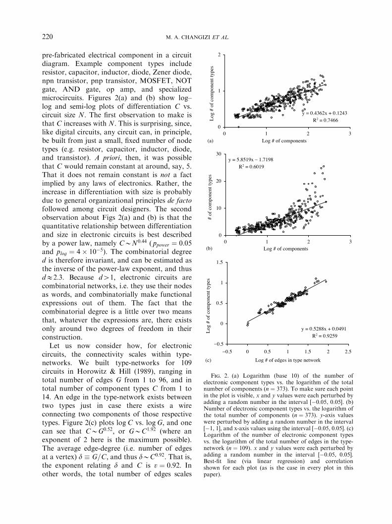
pre-fabricated electrical component in a circuitdiagram. Example component types includeresistor, capacitor, inductor, diode, Zener diode,npn transistor, pnp transistor, MOSFET, NOTgate, AND gate, op amp, and specializedmicrocircuits. Figures 2(a) and (b) show log–log and semi-log plots of differentiation C vs.circuit size N: The first observation to make isthat C increases with N: This is surprising, since,like digital circuits, any circuit can, in principle,be built from just a small, fixed number of nodetypes (e.g. resistor, capacitor, inductor, diode,and transistor). A priori, then, it was possiblethat C would remain constant at around, say, 5.That it does not remain constant is not a factimplied by any laws of electronics. Rather, theincrease in differentiation with size is probablydue to general organizational principles de factofollowed among circuit designers. The secondobservation about Figs 2(a) and (b) is that thequantitative relationship between differentiationand size in electronic circuits is best describedby a power law, namely CBN0:44 ( ppower ! 0:05and plog ! 4( 10&5). The combinatorial degreed is therefore invariant, and can be estimated asthe inverse of the power-law exponent, and thusdE2:3: Because d41; electronic circuits arecombinatorial networks, i.e. they use their nodesas words, and combinatorially make functionalexpressions out of them. The fact that thecombinatorial degree is a little over two meansthat, whatever the expressions are, there existsonly around two degrees of freedom in theirconstruction.Let us now consider how, for electronic

circuits, the connectivity scales within type-networks. We built type-networks for 109circuits in Horowitz & Hill (1989), ranging intotal number of edges G from 1 to 96, and intotal number of component types C from 1 to14. An edge in the type-network exists betweentwo types just in case there exists a wireconnecting two components of those respectivetypes. Figure 2(c) plots logC vs. logG; and onecan see that CBG0:52; or GBC1:92 (where anexponent of 2 here is the maximum possible).The average edge-degree (i.e. number of edgesat a vertex) d ) G=C; and thus dBC0:92: That is,the exponent relating d and C is v ! 0:92: Inother words, the total number of edges scales

y = 0.5288x + 0.0491R2 = 0.9259

_0.5

0

0.5

1

1.5

_0.5 0 0.5 1 1.5 2 2.5Log # of edges in type network

Log

# of

com

pone

nt ty

pes

y = 0.4362x + 0.1243R2 = 0.7466

0

1

2

0 1 2 3Log # of components

Log

# of

com

pone

nt ty

pes

y = 5.8519x _ 1.7198R2 = 0.6019

0

10

20

30

0 1 2 3Log # of components

# of

com

pone

nt ty

pes

(a)

(b)

(c)

Fig. 2. (a) Logarithm (base 10) of the number ofelectronic component types vs. the logarithm of the totalnumber of components (n ! 373). To make sure each pointin the plot is visible, x and y values were each perturbed byadding a random number in the interval [&0.05, 0.05]. (b)Number of electronic component types vs. the logarithm ofthe total number of components (n ! 373). y-axis valueswere perturbed by adding a random number in the interval[&1, 1], and x-axis values using the interval [&0.05, 0.05]. (c)Logarithm of the number of electronic component typesvs. the logarithm of the total number of edges in the type-network (n ! 109). x and y values were each perturbed byadding a random number in the interval [&0.05, 0.05].Best-fit line (via linear regression) and correlationshown for each plot (as is the case in every plot in thispaper).


roughly as quickly as is possible (i.e. it isapproximately the case that GBC2), and thusd scales nearly as fast as possible (i.e. approxi-mately as dBC). Recall that v40 implies thatthe network is acting combinatorially; thisprovides another confirmation of this conclusionmade earlier. Also, using eqn (8) we maycompute L from d and v: L ! "d ' v& 1#=v;and thus L ! "2:3' 0:92& 1#="0:92#E2:43:Because vE1; it follows that LEd; and both Land d are a little over 2.Expressions in electronic circuits therefore

tend to be built out of around two components,and since the combinatorial degree is alsoaround two, it means that all the possibledegrees of freedom are utilized. What mightexpressions in electronic circuits actually be?Introductory electronics books spend consider-able time introducing just such circuits. Forexample, functional circuits found in Horowitz& Hill (1989) include the following (with numberof components and number of component typeswithin the circuit in parentheses):

resistors in series (2, 1), resistors in parallel (2,1), voltage divider (2, 1), adjustable voltagedivider (2, 1), Zener regulator (2, 2), tunneldiode amp (2, 2), RC discharge (2, 2), inte-grator/low-pass filter (2, 2), differentiator/high-pass filter (2, 2), LC resonant/bandpass filter (3,3), LC notch filter (3, 3), half-wave rectifier (1,1), full-wave bridge rectifier (4, 1), full-waverectifier using center-trapped transformer (3, 2),dual-polarity supply (6, 2), voltage doubler (4,2), diode voltage clamp (2, 2), dc restoration (2,2), diode limiter (3, 2), diode drop compensa-tion (4, 2), blocking inductive kick (2, 2), RCsnubber (3, 3), emitter follower (2, 2), Zenervoltage regulator (2, 2), constant-amplitudephase shifter (2, 2), common-emitter amp (2,2), classic bipolar-transistor matched-pair cur-rent mirror (2, 1), improved current mirror (5,2), push-pull emitter follower (2, 2), Darlingtontransistor configuration (2, 1), Sziklai connec-tion (2, 2), classic transistor differential amp (7,2), NMOS logic inverter (2, 2), PMOS logicinverter (2, 2), CMOS logic inverter (2, 1),CMOS NAND gate (4, 1), CMOS linear amp A(3, 3), CMOS linear amp B (5, 3), CMOS linearamp C (5, 3), inverting amp (3, 2), noninvertingamp (3, 2), Howland current source (5, 2),classic differential amp (5, 2), op-amp peak

detector (4, 3), integrator with op-amp (3, 3),negative-impedance converter (3, 2).

One can see that the number of components inmost of these is around two (and that thenumber of types never exceeds three). Our claimis that the combinatorial degree and length ofaround two is the fingerprint of the existence incircuits of these kinds of basic functional entities,or expression types. In less well-understoodkinds of network, the basic functional entitiesmay be unknown, and knowing the combinator-ial degree and length may help to discover whatthey are.

3.2. LEGOS: NETWORKS OF ATTACHABLE PARTS

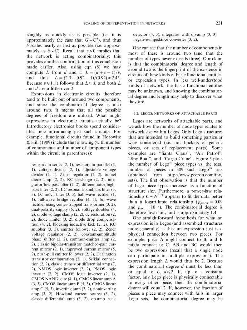
Legos are networks of attachable parts, andwe ask how the number of node types relates tonetwork size within Legos. Only Lego structuresthat are intended to build something particularwere considered (i.e. not buckets of genericpieces, or sets of replacement parts). Someexamples are ‘‘Santa Claus’’, ‘‘Air Patrol’’,‘‘Spy Boat’’, and ‘‘Cargo Crane’’. Figure 3 plotsthe number of Legot piece types vs. the totalnumber of pieces in 389 such Legot sets(obtained from http://www.peeron.com/inv/sets). The first observation is that the numberof Lego piece types increases as a function ofstructure size. Furthermore, a power-law rela-tionship CBN0:71 appears to fit the data betterthan a logarithmic relationship ( ppower ! 0:09and plog ! 10&7). The combinatorial degree istherefore invariant, and is approximately 1.4.One straightforward hypothesis for what an

expression is in Legos (and assembled structuresmore generally) is this: an expression just is aphysical connection between two pieces. Forexample, piece A might connect to B, and Bmight connect to C. AB and BC would thenbe two expressions (recall that a single nodecan participate in multiple expressions). Theexpression length L would thus be 2. Becausethe combinatorial degree d must be less thanor equal to L; dp2: If, up to a constantfactor, any Lego piece is physically connectableto every other piece, then the combinatorialdegree will equal 2. If, however, the fraction ofpieces a piece may connect with falls in largerLego sets, the combinatorial degree may be


lower than 2, and this may explain thelower combinatorial degree of around 1.4.Via similar reasoning, if a network possessedattachments for which m (rather than 2) piecesmust simultaneously physically connect, wewould expect a maximum combinatorial degreeof m:

3.3. BUSINESSES AND UNIVERSITIES:

NETWORKS OF PEOPLE

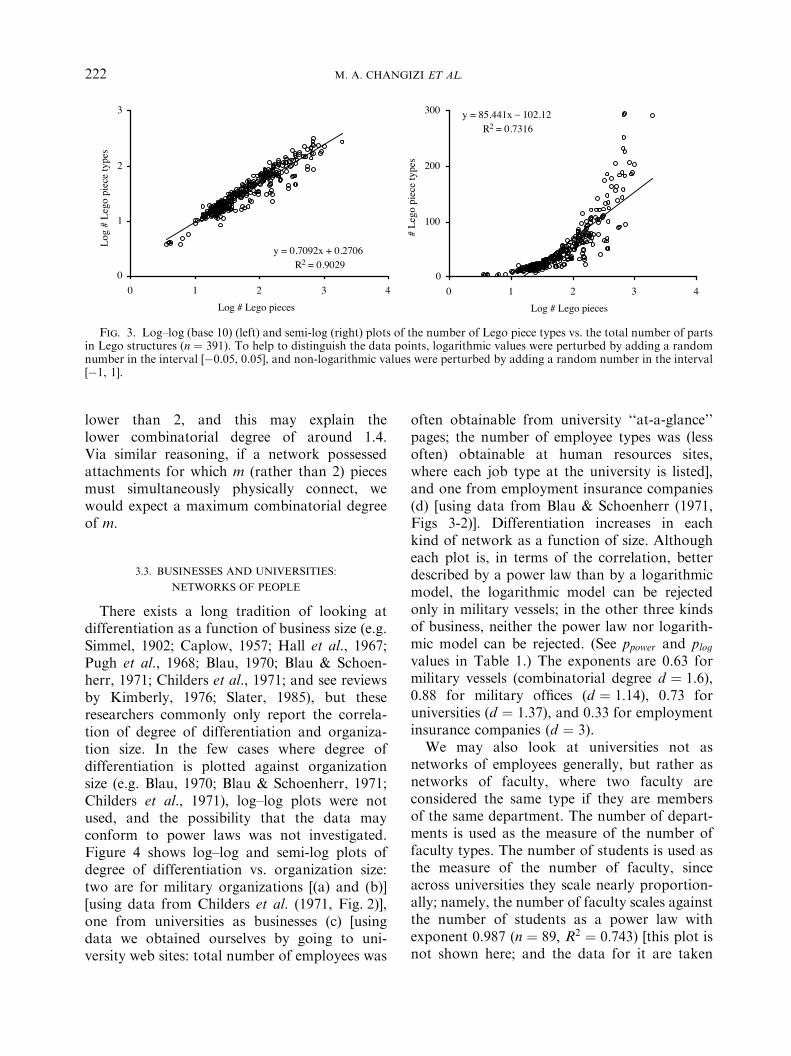
There exists a long tradition of looking atdifferentiation as a function of business size (e.g.Simmel, 1902; Caplow, 1957; Hall et al., 1967;Pugh et al., 1968; Blau, 1970; Blau & Schoen-herr, 1971; Childers et al., 1971; and see reviewsby Kimberly, 1976; Slater, 1985), but theseresearchers commonly only report the correla-tion of degree of differentiation and organiza-tion size. In the few cases where degree ofdifferentiation is plotted against organizationsize (e.g. Blau, 1970; Blau & Schoenherr, 1971;Childers et al., 1971), log–log plots were notused, and the possibility that the data mayconform to power laws was not investigated.Figure 4 shows log–log and semi-log plots ofdegree of differentiation vs. organization size:two are for military organizations [(a) and (b)][using data from Childers et al. (1971, Fig. 2)],one from universities as businesses (c) [usingdata we obtained ourselves by going to uni-versity web sites: total number of employees was

often obtainable from university ‘‘at-a-glance’’pages; the number of employee types was (lessoften) obtainable at human resources sites,where each job type at the university is listed],and one from employment insurance companies(d) [using data from Blau & Schoenherr (1971,Figs 3-2)]. Differentiation increases in eachkind of network as a function of size. Althougheach plot is, in terms of the correlation, betterdescribed by a power law than by a logarithmicmodel, the logarithmic model can be rejectedonly in military vessels; in the other three kindsof business, neither the power law nor logarith-mic model can be rejected. (See ppower and plogvalues in Table 1.) The exponents are 0.63 formilitary vessels (combinatorial degree d ! 1:6),0.88 for military offices (d ! 1:14), 0.73 foruniversities (d ! 1:37), and 0.33 for employmentinsurance companies (d ! 3).We may also look at universities not as

networks of employees generally, but rather asnetworks of faculty, where two faculty areconsidered the same type if they are membersof the same department. The number of depart-ments is used as the measure of the number offaculty types. The number of students is used asthe measure of the number of faculty, sinceacross universities they scale nearly proportion-ally; namely, the number of faculty scales againstthe number of students as a power law withexponent 0.987 (n ! 89; R2 ! 0:743) [this plot isnot shown here; and the data for it are taken

y = 0.7092x + 0.2706R2 = 0.9029

0

1

2

3

0 1 2 3 4Log # Lego pieces

Log

# Le

go p

iece

type

sy = 85.441x _ 102.12

R2 = 0.7316

0

100

200

300

0 1 2 3 4Log # Lego pieces

# Le

go p

iece

type

s

Fig. 3. Log–log (base 10) (left) and semi-log (right) plots of the number of Lego piece types vs. the total number of partsin Lego structures (n ! 391). To help to distinguish the data points, logarithmic values were perturbed by adding a randomnumber in the interval [&0.05, 0.05], and non-logarithmic values were perturbed by adding a random number in the interval[&1, 1].


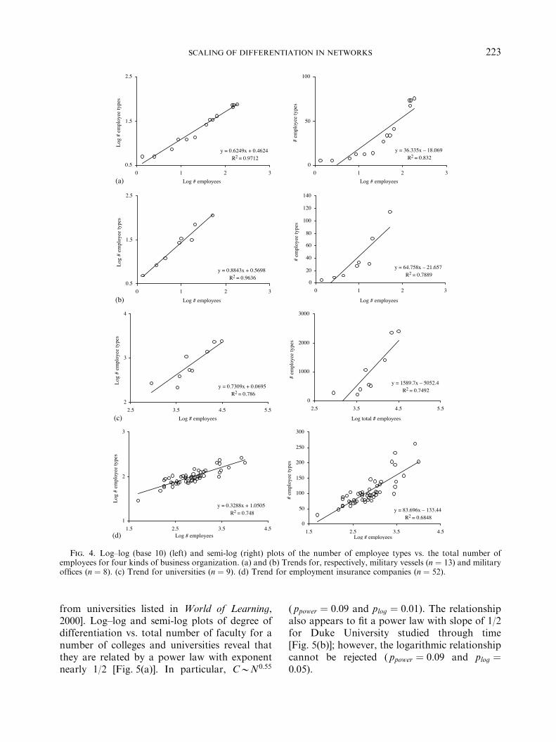
from universities listed in World of Learning,2000]. Log–log and semi-log plots of degree ofdifferentiation vs. total number of faculty for anumber of colleges and universities reveal thatthey are related by a power law with exponentnearly 1/2 [Fig. 5(a)]. In particular, CBN0:55

( ppower ! 0:09 and plog ! 0:01). The relationshipalso appears to fit a power law with slope of 1/2for Duke University studied through time[Fig. 5(b)]; however, the logarithmic relationshipcannot be rejected ( ppower ! 0:09 and plog !0:05).

y = 0.7309x + 0.0695R2 = 0.786

2

3

4

2.5 3.5 4.5 5.5Log # employees

Log

# em

ploy

ee ty

pes

y = 0.6249x + 0.4624R2 = 0.9712

0.5

1.5

2.5

0 1 2 3Log # employees

Log

# em

ploy

ee ty

pes

y = 0.8843x + 0.5698R2 = 0.9636

0.5

1.5

2.5


Log

# em

ploy

ee ty

pes

y = 0.3288x + 1.0505R2 = 0.748

1

2

3


Log

# em

ploy

ee ty

pes

y = 1589.7x _ 5052.4R2 = 0.7492

0

1000

2000

3000

2.5 3.5 4.5 5.5

Log total # employees

# em

ploy

ee ty

pes

y = 36.335x _ 18.069R2 = 0.832

0

50

100


# em

ploy

ee ty

pes

y = 64.758x _ 21.657R2 = 0.7889

0

20

40

60

80

100

120

140

0 1 2 3

Log # employees#

empl

oyee

type

s

y = 83.696x _ 133.44R2 = 0.6848

0

50

100

150

200

250

300


# em

ploy

ee ty

pes

(a)

(b)

(c)

(d)

Fig. 4. Log–log (base 10) (left) and semi-log (right) plots of the number of employee types vs. the total number ofemployees for four kinds of business organization. (a) and (b) Trends for, respectively, military vessels (n ! 13) and militaryoffices (n ! 8). (c) Trend for universities (n ! 9). (d) Trend for employment insurance companies (n ! 52).


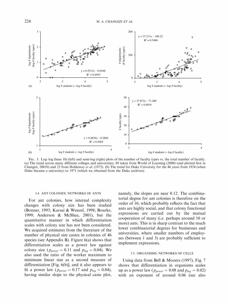
3.4. ANT COLONIES: NETWORKS OF ANTS

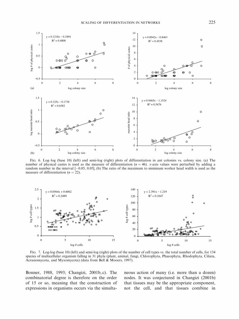
For ant colonies, how internal complexitychanges with colony size has been studied(Bonner, 1993; Karsai & Wenzel, 1998; Bourke,1999; Anderson & McShea, 2001), but thequantitative manner in which differentiationscales with colony size has not been considered.We acquired estimates from the literature of thenumber of physical size castes in colonies of 46species (see Appendix B). Figure 6(a) shows thatdifferentiation scales as a power law againstcolony size ( ppower ! 0:11 and plog ! 0:04). Wealso used the ratio of the worker maximum tominimum linear size as a second measure ofdifferentiation [Fig. 6(b)], and it also appears tofit a power law ( ppower ! 0:17 and plog ! 0:04),having similar slope to the physical caste plot,

namely, the slopes are near 0.12. The combina-torial degree for ant colonies is therefore on theorder of 10, which probably reflects the fact thatants are highly social, and that colony functionalexpressions are carried out by the mutualcooperation of many (i.e. perhaps around 10 ormore) ants. This is in sharp contrast to the muchlower combinatorial degrees for businesses anduniversities, where smaller numbers of employ-ees (between 1 and 3) are probably sufficient toimplement expressions.

3.5. ORGANISMS: NETWORKS OF CELLS

Using data from Bell & Mooers (1997), Fig. 7shows that differentiation in organisms scalesup as a power law ( ppower ! 0:08 and plog ! 0:02)with an exponent of around 0.06 (see also

y = 0.5512x _ 0.6548R2 = 0.6952

0

1

2

3

2 3 4 5log # students (~ log # faculty)

log

# de

partm

ents

(lo

g #

facu

lty ty

pes)

y = 0.4836x _ 0.2884R2 = 0.9205

1

2

3 4log # students (~ log # faculty)

log

# de

partm

ents

(lo

g #

facu

lty ty

pes)

y = 37.311x _ 100.22R2 = 0.5486

0

100

200

2 3 4 5log # students (~ log # faculty)

# de

partm

ents

(#

facu

lty ty

pes)

y = 27.873x _ 71.489R2 = 0.8919

0

10

20

30

40

50

3 4log # students (~ log # faculty)

# fa

culty

type

s

(a)

(b)

Fig. 5. Log–log (base 10) (left) and semi-log (right) plots of the number of faculty types vs. the total number of faculty.(a) The trend across many different colleges and universities, 89 taken from World of Learning (2000) (and plotted first inChangizi, 2001b) and 23 from Holdaway et al. (1975). (b) The trend for Duke University for the 46 years from 1924 (whenDuke became a university) to 1971 (which we obtained from the Duke archives).


Bonner, 1988, 1993; Changizi, 2001b, c). Thecombinatorial degree is therefore on the orderof 15 or so, meaning that the construction ofexpressions in organisms occurs via the simulta-

neous action of many (i.e. more than a dozen)nodes. It was conjectured in Changizi (2001b)that tissues may be the appropriate component,not the cell, and that tissues combine in

y = 0.1218x _ 0.1894R2 = 0.4808

_0.5

0

0.5

1

1.5

0 2 4 6 8

log colony size

log

# of

phy

sica

l cas

tes

y = 0.125x _ 0.1738R2 = 0.6582

_0.5

0

0.5

1

1.5

0 2 4 6 8log colony size

log

max

min

hea

d ra

tio

y = 0.8942x _ 0.8463R2 = 0.4538

0

2

4

6

8

10

12

14

0 2 4 6 8

log colony size

# of

phy

sica

l cas

tes

y = 0.9465x _ 1.1524R2 = 0.5476

0

2

4

6

8

10

12

14

0 2 4 6 8log colony size

max

min

hea

d ra

tio

(a)

(b)

Fig. 6. Log–log (base 10) (left) and semi-log (right) plots of differentiation in ant colonies vs. colony size. (a) Thenumber of physical castes is used as the measure of differentiation (n ! 46). x-axis values were perturbed by adding arandom number in the interval [&0.05, 0.05], (b) The ratio of the maximum to minimum worker head width is used as themeasure of differentiation (n ! 22).

y = 0.0564x + 0.6062R2 = 0.2489

0

0.5

1

1.5

2

2.5

0 5 10 15log # cells

log

# ce

ll ty

pes

y = 2.391x _ 1.219R2 = 0.1647

0

20

40

60

80

100

120

140

0 5 10 15log # cells

log

# ce

ll ty

pes

Fig. 7. Log-log (base 10) (left) and semi-log (right) plots of the number of cell types vs. the total number of cells, for 134species of multicellular organism falling in 31 phyla (plant, animal, fungi, Chlorophyta, Phaeophyta, Rhodophyta, Ciliata,Acrasiomycota, and Myxomycota) (data from Bell & Mooers, 1997).


conglomerations of roughly a dozen (i.e. in therange of 10–20). A combinatorial degree thishigh for organisms is in marked contrast toLegost, where expressions may be built bymerely a pair of physically connecting compo-nents, rather than built by more than a dozenphysically proximal tissues.It is expected that similar combinatorial

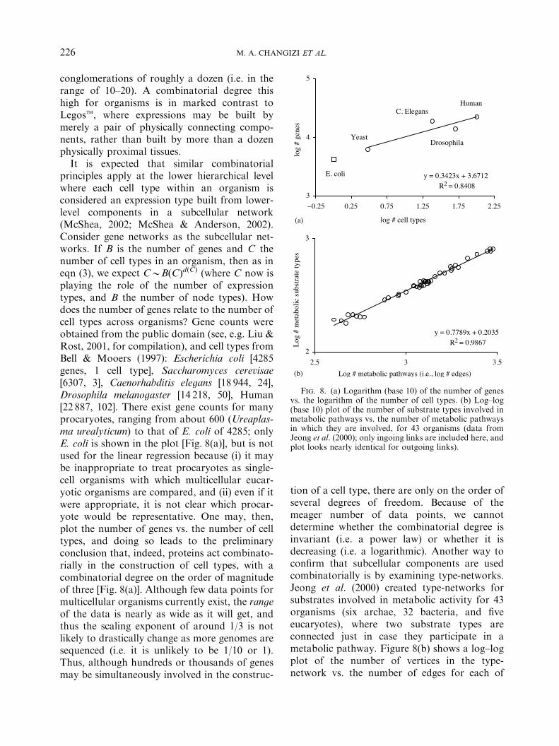
principles apply at the lower hierarchical levelwhere each cell type within an organism isconsidered an expression type built from lower-level components in a subcellular network(McShea, 2002; McShea & Anderson, 2002).Consider gene networks as the subcellular net-works. If B is the number of genes and C thenumber of cell types in an organism, then as ineqn (3), we expect CBB"C#d"C# (where C now isplaying the role of the number of expressiontypes, and B the number of node types). Howdoes the number of genes relate to the number ofcell types across organisms? Gene counts wereobtained from the public domain (see, e.g. Liu &Rost, 2001, for compilation), and cell types fromBell & Mooers (1997): Escherichia coli [4285genes, 1 cell type], Saccharomyces cerevisae[6307, 3], Caenorhabditis elegans [18 944, 24],Drosophila melanogaster [14 218, 50], Human[22 887, 102]. There exist gene counts for manyprocaryotes, ranging from about 600 (Ureaplas-ma urealyticum) to that of E. coli of 4285; onlyE. coli is shown in the plot [Fig. 8(a)], but is notused for the linear regression because (i) it maybe inappropriate to treat procaryotes as single-cell organisms with which multicellular eucar-yotic organisms are compared, and (ii) even if itwere appropriate, it is not clear which procar-yote would be representative. One may, then,plot the number of genes vs. the number of celltypes, and doing so leads to the preliminaryconclusion that, indeed, proteins act combinato-rially in the construction of cell types, with acombinatorial degree on the order of magnitudeof three [Fig. 8(a)]. Although few data points formulticellular organisms currently exist, the rangeof the data is nearly as wide as it will get, andthus the scaling exponent of around 1/3 is notlikely to drastically change as more genomes aresequenced (i.e. it is unlikely to be 1/10 or 1).Thus, although hundreds or thousands of genesmay be simultaneously involved in the construc-

tion of a cell type, there are only on the order ofseveral degrees of freedom. Because of themeager number of data points, we cannotdetermine whether the combinatorial degree isinvariant (i.e. a power law) or whether it isdecreasing (i.e. a logarithmic). Another way toconfirm that subcellular components are usedcombinatorially is by examining type-networks.Jeong et al. (2000) created type-networks forsubstrates involved in metabolic activity for 43organisms (six archae, 32 bacteria, and fiveeucaryotes), where two substrate types areconnected just in case they participate in ametabolic pathway. Figure 8(b) shows a log–logplot of the number of vertices in the type-network vs. the number of edges for each of

y = 0.3423x + 3.6712R2 = 0.8408

3

4

5

_0.25 0.25 0.75 1.25 1.75 2.25

log # cell types

log

# ge

nes

E. coli

Yeast

C. Elegans

Drosophila

Human

y = 0.7789x + 0.2035R2 = 0.9867

2

3

2.5 3 3.5Log # metabolic pathways (i.e., log # edges)

Log

# m

etab

olic

subs

trate

type

s

(a)

(b)

Fig. 8. (a) Logarithm (base 10) of the number of genesvs. the logarithm of the number of cell types. (b) Log–log(base 10) plot of the number of substrate types involved inmetabolic pathways vs. the number of metabolic pathwaysin which they are involved, for 43 organisms (data fromJeong et al. (2000); only ingoing links are included here, andplot looks nearly identical for outgoing links).


these organisms, and one can see that thenumber of subcellular node types B scales asthe number of edges G in the type-network to thepower of 0.78, or GBB1:28 (where, recall, anexponent of 2 is the maximum possible). Theaverage edge-degree (i.e. the number of edges ata vertex) d ) G=B; and thus dBB 0:28: Therefore,v ! 0:28; and since v40 it implies that metabolicnetworks act combinatorially.

3.6. NERVOUS SYSTEMS: NETWORKS OF NEURONS

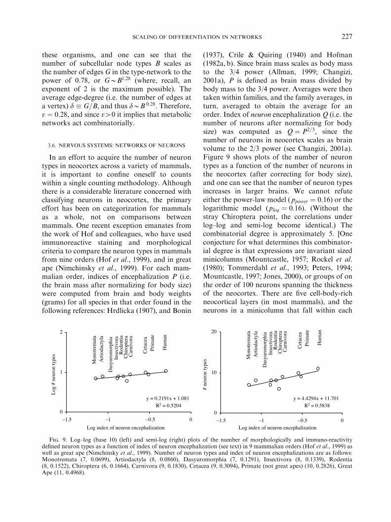
In an effort to acquire the number of neurontypes in neocortex across a variety of mammals,it is important to confine oneself to countswithin a single counting methodology. Althoughthere is a considerable literature concerned withclassifying neurons in neocortex, the primaryeffort has been on categorization for mammalsas a whole, not on comparisons betweenmammals. One recent exception emanates fromthe work of Hof and colleagues, who have usedimmunoreactive staining and morphologicalcriteria to compare the neuron types in mammalsfrom nine orders (Hof et al., 1999), and in greatape (Nimchinsky et al., 1999). For each mam-malian order, indices of encephalization P (i.e.the brain mass after normalizing for body size)were computed from brain and body weights(grams) for all species in that order found in thefollowing references: Hrdlicka (1907), and Bonin

(1937), Crile & Quiring (1940) and Hofman(1982a, b). Since brain mass scales as body massto the 3/4 power (Allman, 1999; Changizi,2001a), P is defined as brain mass divided bybody mass to the 3/4 power. Averages were thentaken within families, and the family averages, inturn, averaged to obtain the average for anorder. Index of neuron encephalization Q (i.e. thenumber of neurons after normalizing for bodysize) was computed as Q ! P2=3; since thenumber of neurons in neocortex scales as brainvolume to the 2/3 power (see Changizi, 2001a).Figure 9 shows plots of the number of neurontypes as a function of the number of neurons inthe neocortex (after correcting for body size),and one can see that the number of neuron typesincreases in larger brains. We cannot refuteeither the power-law model ( ppower ! 0:16) or thelogarithmic model (plog ! 0:16). (Without thestray Chiroptera point, the correlations underlog–log and semi-log become identical.) Thecombinatorial degree is approximately 5. [Oneconjecture for what determines this combinator-ial degree is that expressions are invariant sizedminicolumns (Mountcastle, 1957; Rockel et al.(1980); Tommerdahl et al., 1993; Peters, 1994;Mountcastle, 1997; Jones, 2000), or groups of onthe order of 100 neurons spanning the thicknessof the neocortex. There are five cell-body-richneocortical layers (in most mammals), and theneurons in a minicolumn that fall within each

y = 0.2191x + 1.081R2 = 0.5204

0

1

2

_1.5 _1 _0.5 0Log index of neuron encephalization

Log

# ne

uron

type

s

Arti

odac

tyla

Mon

otre

mat

a

Das

yuro

mor

phia

Inse

ctiv

ora

Rod

entia

Chi

ropt

era

Car

nivo

ra

Cet

acea

Prim

ate

Hum

an

y = 4.4294x + 11.701R2 = 0.5838

0

10

20

_1.5 _1 _0.5 0Log index of neuron encephalization

# ne

uron

type

s

Arti

odac

tyla

Mon

otre

mat

a

Das

yuro

mor

phia

Inse

ctiv

ora

Rod

entia

Chi

ropt

era

Car

nivo

ra

Cet

acea

Prim

ate

Hum

an

Fig. 9. Log–log (base 10) (left) and semi-log (right) plots of the number of morphologically and immuno-reactivitydefined neuron types as a function of index of neuron encephalization (see text) in 9 mammalian orders (Hof et al., 1999) aswell as great ape (Nimchinsky et al., 1999). Number of neuron types and index of neuron encephalizations are as follows:Monotremata (7, 0.0699), Artiodactyla (8, 0.0860), Dasyuromorphia (7, 0.1291), Insectivora (8, 0.1339), Rodentia(8, 0.1522), Chiroptera (6, 0.1664), Carnivora (9, 0.1830), Cetacea (9, 0.3094), Primate (not great apes) (10, 0.2826), GreatApe (11, 0.4968).


layer may serve a distinct role in the functioningof a minicolumn. The conjecture is, then, thatthese five layers provide five degrees of freedomin the construction of a minicolumn, which isreflected in the way the number of neuron typesscales with brain size.]Another nervous system for which consider-

able data exist on the number of neuron types isthe vertebrate retina. As was the case for theneocortex, less attention has been paid tocomparing the number of neuron types acrossdifferent animals, but the research of Kalloniatisand Marc provides a single methodology inwhich counts have been made for three animals.The method uses pattern recognition of aminoacid signals to make the classifications, andcounts are nine neuron types for goldfish(Carassius auratus) (Marc et al., 1995), 12 forcat (Marc et al., 1998), and 15 for primate(Kalloniatis et al., 1996). [These counts do notinclude retinal pigment epithelial cells or glialcells (e.g. Muller cells).] The index of neuronencephalizations for the three animals are,respectively, 0.0689, 0.1830, 0.3374 (computedfrom data in the sources and in the manner givenabove for neocortex). A log–log plot of numberof retinal types vs. index of neuron encephaliza-tion (not shown) gives a best-fit equation ofy ! 0:319x' 1:322; and R2 ! 0:9965: Becauseof the small number of data points, and becauseindex of neocortical neuron encephalization isnot an appropriate measure of the number ofneurons in the retina, we attempt no analysisof these data, except to say that it is clearthat the number of neuron types does appearto increase in retina of more complexanimals.

3.7. COMPETITIVE NETWORKS:

ECOSYSTEMS AND CITIES

The scaling of differentiation has receivedconsiderable attention in ecosystems, wherethere is a long history of studying how thenumber of organism types (i.e. species) scales upwith the area of the land, going back at least toWatson in 1859 (Williams, 1964; Rosenzweig,1995). Since land area A scales proportionally tothe number of organisms N; species–area plotsserve as plots of the number of organism types C

vs. the total number of organisms N: There aremany kinds of species–area plot (e.g. seeRosenzweig, 1995, p. 8), and we are here onlyinterested in those which study how differentia-tion scales across networks of different sizes, incontrast to studies of larger and larger subsets ofa single network (as in quadrat studies) wherethe governing principles can be distinct. What isan ecosystem network? The best candidate is anisland biota, as (i) an island is a well-demarcatednetwork of organisms, (ii) archipelagos usefullyserve to identify a group of such networks ofsimilar kind, and (iii) island species–area studiesare not beset with sampling issues as is the casein some of the other kinds of species–areastudies. Accordingly, we wish to know how thenumber of species scales up as a function ofisland size among islands within an archipelago.Many such studies have been carried out, usuallyfocusing on just one class of organism (e.g.Wilson, 1961; MacArthur & Wilson, 1963;Johnson et al., 1968; Brown, 1971; Diamond,1972, 1974; Power, 1972; Johnson & Simberloff,1974; Case, 1975; Johnson, 1975; Diamond &Mayr, 1976; Simberloff, 1976; Connor &McCoy, 1979; Wright, 1981; Lomolino, 1982;Heaney, 1984; Losos, 1996; Nieminen, 1996;Holt et al., 1999; Losos & Schluter, 2000). Onthe whole, such species–area plots conform topower laws with slopes in the approximate rangeof 0.2–0.4 (Rosenzweig, 1995). For example,Connor & McCoy (1979) cataloged 100 suchslopes from the literature, and among theroughly 60 island slopes, the average is about0.3.Why is differentiation and network size

related by a power law in island biota networks?We explained the power-law relationship forselected networks via the Minimal N Hypoth-esis, but as discussed then, the hypothesis is onlyplausible for selected networks. Island biotanetworks are competitive networks (where selec-tion acts at the level of the nodes, not at the levelof the entire network), not selected networks,and the Minimal N Hypothesis is inappropriate.However, there is another hypothesis that isplausible for island biota networks. Beforestating the hypothesis, consider that a group oforganisms can interact in such a way as to filla habitat. That is, some particular group of


organisms may be able, by virtue of theirinteractions, to invade a certain kind of habitat,whereas another group of organisms (made upof different organism types) may not be able to.These habitat-filling groups of organisms areexpressions in the network. We make thefollowing Habitat-Filling Hypothesis, whichstates that, up to a constant proportion, everyhabitat type is filled by an expression type (i.e.filled by a type of group of interacting organisms).The motivation for this hypothesis is that,because of competition in the network, everykind of habitat will be invaded. From this wemay derive that the number of habitat types, H;will scale proportionally with the number ofexpression types, E (i.e. E is the number ofdifferent ways groups of organisms interact tofill habitats). That is, HBE: Since islands withtwice the area, A; tend to have roughly twice thenumber of habitat types, H; we may derive thatABE: Recalling that island area, A; is propor-tional to network size, N; we may conclude thatNBE: (Note also that since NX$L"E#=s%E fromeqn (1), it follows that L is invariant.) Recallthat this was eqn (2). In a manner identical tothat in Section 2, we may now go on to derivethat, for island biota networks, eqn (5) holds.Namely,

NBCd ; where d is invariant andX1:

We have arrived at the same conclusion as wedid for selected networks, but we have doneso using a different explanation. A power-lawrelationship holds for island biota networks notbecause such networks optimize their size subjectto the ‘‘needed’’ network complexity (as was thecase for selected networks), but, rather, becausethese networks maximally fill every availablehabitat (up to a constant factor) on the island.[This explanation of the species–area relation-ship has certain affinities with Williams (1964)and Simberloff (1972) in that the number oforganism types is hypothesized to increasebecause of the increase in the number of habitattypes.]Although we have just provided an explana-

tion for why species–area plots conform topower laws, we have not explained the magni-tude of the exponent. As mentioned earlier, the

power-law exponents for species–area plots tendto be approximately 0.3, and thus the combina-torial degree values are around 3 (ranging fromabout 2.5 to 5, depending on the study). We nowput forth an explanation for why combinatorialdegrees are in this range. A combinatorial degreeof around 3 means that there are three degrees offreedom in expressions, recalling that expres-sions are habitat-filling groups of organisms. Wehypothesize that such habitat-filling groups areof the following nature: each group consists ofa predator, a herbivorous prey, and so on downthrough the trophic levels. That is, we hypothe-size that expressions are food chains, and it isfood chains that fill habitats. Furthermore, wehypothesize that there is a degree of freedom foreach trophic level in the chain, and thus that thecombinatorial degree is determined by foodchain length. This hypothesis makes severalpredictions.One straightforward prediction is that, since

the combinatorial degrees are roughly 3 (i.e.somewhere between 2.5 and 5), food chainlengths should also be around 3 on average(i.e. somewhere between 2.5 and 5). Food chainlengths have been measured in a variety of kindsof food web (Pimm & Lawton, 1977; Briand,1983; May, 1983; Cohen et al., 1986, 1990;Newman & Cohen, 1986; Schoener, 1989;Sugihara et al., 1989; Warren, 1989; Martinez,1991; Pimm et al., 1991; Polis, 1991; Schoenlyet al., 1991; Goldwasser & Roughgarden, 1993,1997; Cabana & Rasmussen, 1996; VanderZanden et al., 1999; Post et al., 2000), and,indeed, their lengths tend to be in the range ofabout 3–5 (for longer estimates see Polis, 1991;Martinez, 1991). For example, of 113 webs inCohen et al. (1990), the average of the averagefood chain length within a web is 2.88 (S.D.0.87), and the average maximum chain length is4.21 (S.D. 1.51). More recent isotope methodsfor determining the number of trophic levels (inaquatic systems) have concluded that there arebetween 3 and 5 (Cabana & Rasmussen, 1996;Vander Zanden et al., 1999; Post et al., 2000).These food chain length estimates are, then,consistent with the hypothesis that it is foodchains that are the expressions, and that thecombinatorial degree is determined by the foodchain length.


A second prediction of this ‘‘combinatorialdegree dEfood chain length L’’ hypothesis isthat, since the combinatorial degree is invariant,food chain length should not vary as a functionof island area. Although food chain length doesappear to increase somewhat as a function ofspecies richness (Briand, 1983; Hall & Raffaelli,1991; Vander Zanden et al., 1999; Post et al.,2000), we are unaware of any documentedtrend in food chain length as a function ofisland size.We may make a third prediction by recalling

eqn (7) from Subsection 2.5, which stated thatd ! vL& v' 1; where v is the scaling exponentrelating edge-degree d to the number of verticesC in a type-network. This may be manipulatedto become v ! "d & 1#="L& 1#: Our hypothesisthat dEL (and each is 41) for island biotanetworks predicts that v ! 1: For ecosystems,type-networks are food webs, and edges aretrophic links. Our prediction is therefore that, infood webs, the number of trophic links perspecies, or edge-degree d; scales proportionallywith the number of species in the web, C: Theearliest studies of edge-degree scaling arguedthat dBC0 (e.g. Pimm, 1982; Cohen & Briand,1984; Sugihara et al., 1989; Cohen et al., 1990;Warren, 1990), meaning v ! 0: (This wouldimply that island biota networks are notcombinatorial at all.) Later researchers, how-ever, suggested that such edge-degree invariancemay primarily be due to ‘‘artistic convenience’’in drawing food webs, and that more detailedfood webs reveal that v40: for example, Pimmet al. (1991) give v ! 0:3 or 0.4, Havens (1992)gives v ! 0:4; and Martinez (1992), Deb (1995),and Havens (1997) argue that v ! 1: These mostrecent estimates are consistent with our predic-tion. If, however, v is sometimes lower than 1,then it would imply that food chain length isgreater than the combinatorial degree [again, asrelated by eqn (7)].Finally, notice that if this ‘‘combinatorial

degree E food chain length’’ hypothesis is true,then archipelagos with longer food chains arepredicted to have lower species–area slopes, allthings equal. This is because biota with longerchains have more combinatorial room to buildnovel expression types with which to fill newhabitat types without the need for new species;

biota with shorter chains exhaust their possibleexpression types more quickly, and a neworganism type (via speciation or invasion) isneeded in order to have new expression typescapable of adjusting to novel habitat types. Acounterintuitive consequence of this is that ifhealthier biotas tend to have longer food chains(e.g. of length 5 rather than, say, 3), thenhealthier biotas should scale up the number ofspecies less quickly than less healthy biota withshorter chains, all things equal.Another kind of competitive network is cities,

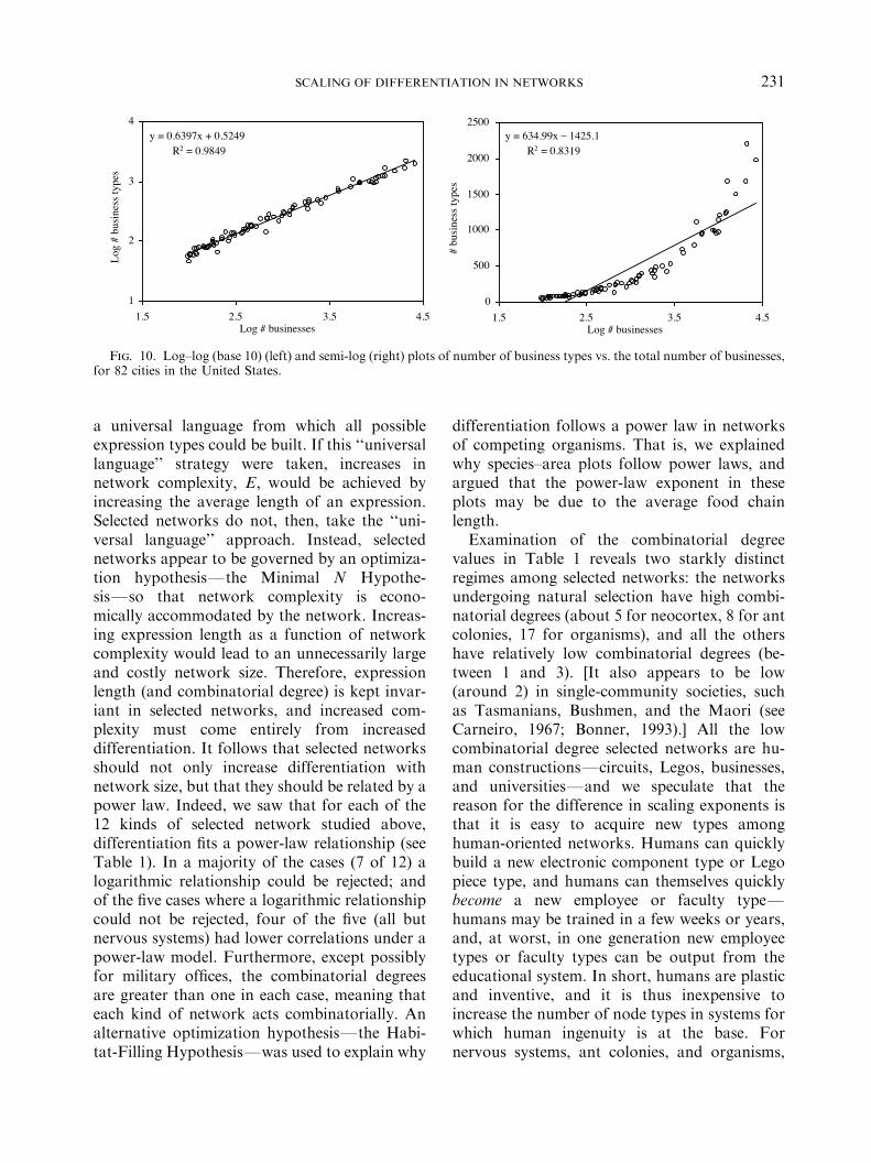
or networks of businesses. Using web-accessiblebusiness directories (i.e. online yellow pages), for82 cities we measured the number of businessesin the city N and the number of types, orcategories, of business C: The cities were chosenarbitrarily, the only guide being to acquire alarge range of city sizes. Data were obtained viathe online search engine www.superpages.gte.-net. The search engine allows one to search forall businesses and all business types amongbusinesses whose first letter is a certain char-acter. Searches via very common first-lettercharacters lead to too many listings and theengine responds with an ‘‘error’’, so we carriedout searches using the relatively less commonfirst-letter characters ‘j’ and ‘k’. Figure 10 showsthe results for ‘j’ (the plots for ‘k’, not shown,look nearly identical), and the differentiation ofa city increases roughly as CBN0:64: Note thatthis kind of scaling law is important to know forthose wishing to use economic diversity mea-sures to diagnose a city’s economic health: anygood measure of economic diversity would haveto account for the diversity that is due simply tothe city being as large as it is, and an appropriatemeasure might accordingly be C=N0:64: We donot take up here possible explanations for thisscaling relationship.

4. Discussion and Conclusion

Consider some of the generalizations we maymake about the scaling of differentiation inselected networks. The first, and most central,generalization is that differentiation increaseswith size. This is not some kind of tautology, foras discussed in Section 1, it is a priori possiblethat a fixed set of node types could serve as


a universal language from which all possibleexpression types could be built. If this ‘‘universallanguage’’ strategy were taken, increases innetwork complexity, E; would be achieved byincreasing the average length of an expression.Selected networks do not, then, take the ‘‘uni-versal language’’ approach. Instead, selectednetworks appear to be governed by an optimiza-tion hypothesisFthe Minimal N Hypothe-sisFso that network complexity is econo-mically accommodated by the network. Increas-ing expression length as a function of networkcomplexity would lead to an unnecessarily largeand costly network size. Therefore, expressionlength (and combinatorial degree) is kept invar-iant in selected networks, and increased com-plexity must come entirely from increaseddifferentiation. It follows that selected networksshould not only increase differentiation withnetwork size, but that they should be related by apower law. Indeed, we saw that for each of the12 kinds of selected network studied above,differentiation fits a power-law relationship (seeTable 1). In a majority of the cases (7 of 12) alogarithmic relationship could be rejected; andof the five cases where a logarithmic relationshipcould not be rejected, four of the five (all butnervous systems) had lower correlations under apower-law model. Furthermore, except possiblyfor military offices, the combinatorial degreesare greater than one in each case, meaning thateach kind of network acts combinatorially. Analternative optimization hypothesisFthe Habi-tat-Filling HypothesisFwas used to explain why

differentiation follows a power law in networksof competing organisms. That is, we explainedwhy species–area plots follow power laws, andargued that the power-law exponent in theseplots may be due to the average food chainlength.Examination of the combinatorial degree

values in Table 1 reveals two starkly distinctregimes among selected networks: the networksundergoing natural selection have high combi-natorial degrees (about 5 for neocortex, 8 for antcolonies, 17 for organisms), and all the othershave relatively low combinatorial degrees (be-tween 1 and 3). [It also appears to be low(around 2) in single-community societies, suchas Tasmanians, Bushmen, and the Maori (seeCarneiro, 1967; Bonner, 1993).] All the lowcombinatorial degree selected networks are hu-man constructionsFcircuits, Legos, businesses,and universitiesFand we speculate that thereason for the difference in scaling exponents isthat it is easy to acquire new types amonghuman-oriented networks. Humans can quicklybuild a new electronic component type or Legopiece type, and humans can themselves quicklybecome a new employee or faculty typeFhumans may be trained in a few weeks or years,and, at worst, in one generation new employeetypes or faculty types can be output from theeducational system. In short, humans are plasticand inventive, and it is thus inexpensive toincrease the number of node types in systems forwhich human ingenuity is at the base. Fornervous systems, ant colonies, and organisms,

y = 0.6397x + 0.5249R2 = 0.9849

1

2

3

4

1.5 2.5 3.5 4.5Log # businesses

Log

# bu

sine

ss ty

pes

y = 634.99x _ 1425.1R2 = 0.8319

0

500

1000

1500

2000

2500

1.5 2.5 3.5 4.5Log # businesses

# bu

sine

ss ty

pes

Fig. 10. Log–log (base 10) (left) and semi-log (right) plots of number of business types vs. the total number of businesses,for 82 cities in the United States.


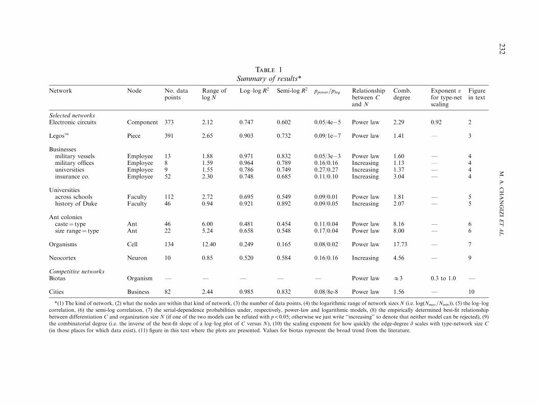
Table 1Summary of results*

Network Node No. datapoints

Range oflogN

Log–logR2 Semi-logR2 ppower=plog Relationshipbetween Cand N

Comb.degree

Exponent vfor type-netscaling

Figurein text

Selected networksElectronic circuits Component 373 2.12 0.747 0.602 0.05/4e&5 Power law 2.29 0.92 2

Legost Piece 391 2.65 0.903 0.732 0.09/1e&7 Power law 1.41 F 3

Businessesmilitary vessels Employee 13 1.88 0.971 0.832 0.05/3e&3 Power law 1.60 F 4military offices Employee 8 1.59 0.964 0.789 0.16/0.16 Increasing 1.13 F 4universities Employee 9 1.55 0.786 0.749 0.27/0.27 Increasing 1.37 F 4insurance co. Employee 52 2.30 0.748 0.685 0.11/0.10 Increasing 3.04 F 4

Universitiesacross schools Faculty 112 2.72 0.695 0.549 0.09/0.01 Power law 1.81 F 5history of Duke Faculty 46 0.94 0.921 0.892 0.09/0.05 Increasing 2.07 F 5

Ant coloniescaste! type Ant 46 6.00 0.481 0.454 0.11/0.04 Power law 8.16 F 6size range! type Ant 22 5.24 0.658 0.548 0.17/0.04 Power law 8.00 F 6

Organisms Cell 134 12.40 0.249 0.165 0.08/0.02 Power law 17.73 F 7

Neocortex Neuron 10 0.85 0.520 0.584 0.16/0.16 Increasing 4.56 F 9

Competitive networksBiotas Organism F F F F F Power law E3 0.3 to 1.0 F

Cities Business 82 2.44 0.985 0.832 0.08/8e-8 Power law 1.56 F 10

*(1) The kind of network, (2) what the nodes are within that kind of network, (3) the number of data points, (4) the logarithmic range of network sizes N (i.e. log"Nmax=Nmin#), (5) the log–logcorrelation, (6) the semi-log correlation, (7) the serial-dependence probabilities under, respectively, power-law and logarithmic models, (8) the empirically determined best-fit relationshipbetween differentiation C and organization size N (if one of the two models can be refuted with po0:05; otherwise we just write ‘‘increasing’’ to denote that neither model can be rejected), (9)the combinatorial degree (i.e. the inverse of the best-fit slope of a log–log plot of C versus N), (10) the scaling exponent for how quickly the edge-degree d scales with type-network size C(in those places for which data exist), (11) figure in this text where the plots are presented. Values for biotas represent the broad trend from the literature.

M.A.CHANGIZ

IETAL.

232

on the other hand, the creation of a new nodetype is costly and difficult: natural selection isrequired. Having a greater combinatorial degreedrastically reduces the rate at which new nodetypes must be added. However, this comes witha cost: each expression itself must be morecomplex. That is, more components must inter-act in a coordinated, or social, manner in orderthat an expression be implemented. This is onereason that even small nervous systems, antcolonies, and organisms are so much moredifficult to understand than, say, (similarly sized)electronic circuits: their expressions are longer,and the rules governing the formation ofexpressions are accordingly more difficult toinfer.

The authors thank Drs Daniel McShea, RichardBurton, Warren G. Hall, and Zhi-Yong Yang forvaluable discussions and comments.

REFERENCES

Allman, J. M. (1999). Evolving Brains. New York:Scientific American Library.

Anderson, C. & McShea, D. W. (2001). Individual versussocial complexity, with particular reference to antcolonies. Biol. Rev. 76, 211–237.

Ash, R. B. (1965). Information Theory. New York: Dover.Bara! basi, A.-L. & Albert, R. (1999). Emergence ofscaling in random networks. Science 286, 509–512.

Bell, G. & Mooers, A. O. (1997). Size and complexityamong multicellular organisms. Biol. J. Linn. Soc. 60,345–363.

Beshers, S. N. & Traniello, J. F. A. (1994). Theadaptiveness of worker demography in the Attine andTrachymyrmex septentrionalis. Ecology 75, 763–775.

Blau, P. M. (1970). A formal theory of differentiation inorganizations. Am. Sociol. Rev. 35, 201–218.

Blau, P. M. & Schoenherr, P. M. (1971). The Structure ofOrganizations. New York: Basic Books.

Bonin, G. von. (1937). Brain-weight and body-weight ofmammals. J. Gen. Psychol. 16, 379–389.

Bonner, J. T. (1988). The Evolution of Complexity.Princeton, NJ: Princeton University Press.

Bonner, J. T. (1993). Dividing the labour in cells andsocieties. Curr. Sci. 64, 459–466.

Bourke, A. F. G. (1999). Colony size, social complexityand reproductive conflict in social insects. J. Evol. Biol.12, 245–257.

Branda‹ o, C. R. F. (1978). Division of labor with theworker caste of Formica perpilosa Wheeler (Hymen-optera: Formicidae). Psyche 85, 229–337.

Branda‹ o, C. R. F. (1983). Sequential ethograms alongcolony development of Odontomachus affinis Gu!erin(Hymenoptera, Formicidae, Ponerinae). Insectes Soc.30, 193–203.

Briand, F. (1983). Environmental control of food webstructure. Ecology 64, 253–263.

Brown, J. H. (1971). Mammals on mountaintops: none-quilibrium insular biogeography. Am. Nat. 105, 467– 478.

Cabana, G. & Rasmussen, J. B. (1996). Comparison ofaquatic food chains using nitrogen isotopes. Proc. NatlAcad. Sci. U.S.A. 93, 10 844–10 847.

Caplow, T. (1957). Organizational size. Admin. Sci. Q. 1,484–505.

Carlin, N. F. (1981). Polymorphism and division of laborin the Dacetine ant Orectogmathus versicolor (Hymen-optera: Formicidae). Psyche 88, 231–244.

Carneiro, R. L. (1967). On the relationship between sizeof population and complexity of social organization.Southwestern J. Anthropol. 23, 234–243.

Case, T. J. (1975). Species numbers, density compensation,and colonizing ability of lizards on islands in the Gulf ofCalifornia. Ecology 56, 3–18.

Changizi, M. A. (2001a). Principles underlying mamma-lian neocortical scaling. Biol. Cybern. 84, 207–215.

Changizi, M. A. (2001b). Universal scaling laws forhierarchical complexity in languages, organisms, beha-viors and other combinatorial systems. J. theor. Biol. 211,277–295.

Changizi, M. A. (2001c). Universal laws for hierarchicalsystems. Comments on Theor. Biol. 6, 25–75.

Changizi, M. A. (2001d). The economy of the shape oflimbed animals. Biol. Cybern. 84, 23–29.

Changizi, M. A. The Brain from 25,000 Feet: High LevelExplorations of Brain Complexity, Perception, Induction,and Vagueness. Dordrecht: Kluwer Academic, in press.

Changizi, M. A. & Cherniak, C. (2000). Modeling thelarge-scale geometry of human coronary arteries. Can.J. Physiol. Pharmacol. 78, 603–611.

Cherniak, C., Changizi, M. A. & Kang, D. (1999).Large-scale optimization of neuron arbors. PhysicalReview E 59, 6001–6009.

Childers, G. W., Mayhew, B. H. Jr. & Gray, L. N.(1971). System size and structural differentiation inmilitary organizations: testing a baseline model ofdivision of labor. Am. J. Sociol. 76, 813–830.

Cohen, J. E. & Briand, F. (1984). Trophic links incommunity food webs. Proc. Natl Acad. Sci. U.S.A. 81,4105–4109.

Cohen, J. E., Briand, F. & Newman, C. M. (1986). Astochastic theory of community food webs. III. Predictedand observed lengths of food chains. Proc. R. Soc.London B 228, 317–353.

Cohen, J. E., Briand, F. & Newman, C. M. (1990).Community Food Webs. Data and Theory. New York:Springer-Verlag.

Connor, E. F. & McCoy, E. D. (1979). The statistics andbiology of the species–area relationship. Am. Nat. 113,791–833.

Corn, M. L. (1980). Polymorphism and polyethism inthe neotropical ant Cephalotes atratus. Insectes Soc. 27,29–42.

Crile, G. & Quiring, D. P. (1940). A record of the bodyweight and certain organ and gland weights of 3690animals. Ohio J. Sci. 40, 219–259.

Deb, D. (1995). Scale-dependence of food web structures:tropical ponds as paradigm. Oikos 72, 245–262.


Diamond, J. M. (1972). Biogeographic kinetics: estimationof relaxation times for avifaunas of southwest Pacificislands. Proc. Natl Acad. Sci. U.S.A. 69, 3199–3203.

Diamond, J. M. (1974). Colonization of exploded volcanicislands by birds: the supertramp strategy. Science 184,803–806.

Diamond, J. M. & Mayr, E. (1976). Species–area relationfor birds of the Solomon Archipelago. Proc. Natl Acad.Sci. U.S.A. 73, 262–266.

Fowler, H. G., Pereira-da-Silva, S., Forti, L. C. &Saes, N. B. (1986). Population dynamics of leaf cuttingants: a brief review. In: Fire Ants and Leaf Cutting Ants:Biology and Management (Lofgren, C. S. & Vander Meer,R. K., eds), pp. 18–35. Boulder: Westview Press.

Franks, N. R. Reproduction, foraging efficiency andworker polymorphism in army ants. In: ExperimentalBehavioural Ecology and Sociobiology Fortschr. Zool.(Holldobler, B. & Lindauer, M., eds), 31, 91–107, 1985.

Franks, N. R. & Norris, P. J. (1986). Constraints on thedivision of labor in ants: D’Arcy Thompson cartesiantransformations applied to worker polymorphism. In:From Individual Characteristics to Collective Organiza-tion, the Example of Social Insects (Pasteels, J. M. &Deneubourg, J. L., eds), Experentia (supplement).

Goldwasser, L. & Roughgarden, J. (1993). Construc-tion and analysis of a large Caribbean food web. Ecology74, 1216–1233.

Goldwasser, L. & Roughgarden, J. (1997). Samplingeffects and the estimation of food-web properties.Ecology 78, 41–54.

Hall, R. H., Haas, J. E. & Johnson, N. J. (1967).Organizational size, complexity, and formalization. Am.Sociol. Rev. 32, 903–912.

Hall, S. J. & Raffaelli, D. (1991). Food-web patterns:lessons from a species-rich web. J. Anim. Ecol. 60,823–842.

Havens, K. (1992). Scale and structure in natural foodwebs. Science 257, 1107–1109.

Havens, K. E. (1997). Unique structural properties ofpelagic food webs. Oikos 78, 75–80.

Heaney, L. R. (1984). Mammalian species richness onislands on the Sunda Shelf, Southeast Asia. Oecologia 61,11–17.

Hof, P. R., Glezer, I. I., Conde¤ , F., Flagg, R. A.,Rubin, M. B., Nimchinsky, E. A., Weisenhorn, D. M. V.(1999). Cellular distribution of the calcium-bindingproteins parvalbumin, calbindin, and calretinin in theneocortex of mammals: phylogenetic and developmentalpatterns. J. Chem. Neuroanat. 16, 77–116.

Hofman, M. A. (1982a). Encephalization in mammals inrelation to the size of the cerebral cortex. Brain Behav.Evol. 20, 84–96.

Hofman, M. A. (1982b). A two-component theory ofencephalization in mammals. J. theor. Biol. 99, 571–584.

Holdaway, E. A., Newberry, J. F., Hickson, D. J. &Heron, R. P. (1975). Dimensions of organizations incomplex societies: the educational sector. Admin. Sci. Q.20, 37–58.

Holt, R. D., Lawton, J. H., Polis, G. A. & Martinez,N. D. Trophic rank and the species–area relationship.Ecology 80, 1495–1504.

Horowitz, P. & Hill, W. (1989). The Art of Electronics.Cambridge: Cambridge University Press.

Hrdlicka, A. (1907). Brain Weight in Vertebrates,Smithsonian Miscellaneous Collections, pp. 89–112.Washington, D.C.: Smithsonian.

Jaffe, K. (1987). Evolution of territoriality and nestmaterecognition systems in ants. In: From Individual toCollective Behavior in Social Insects (Pasteels, J. M. &Deneubourg, J. L., eds), pp. 295–311. Basel: Birkh.auserVerlag.

Jeong, H., Tombor, B., Albert, R., Oltvai, Z. N. &Barab !asi, A.-L. (2000). The large-scale organization ofmetabolic networks. Nature 407, 651–654.

Johnson, M. P. & Simberloff, D. S. (1974). Environ-mental determinants of island species numbers in theBritish Isles. J. Biogeogr. 1, 149–154.

Johnson, M. P., Mason, L. G. & Raven, P. H. (1968).Ecological parameters and plant species diversity. Am.Nat. 102, 297–306.

Johnson, N. K. (1975). Controls of number of bird specieson montane islands in the Great Basin. Evolution 29,545–567.

Jones, E. G. (2000). Microcolumns in the cerebral cortex.Proc. Natl Acad. Sci. U.S.A. 97, 5019–5021.

Kalloniatis, M., Marc, R. E. & Murry, R. F. (1996).Amino acid signatures in the primate retina. J. Neurosci.16, 6807–6829.

Karsai, I. & Wenzel, J. W. (1998). Productivity, indivi-dual-level and colony-level flexibility, and organization ofwork as consequences of colony size. Proc. Natl Acad.Sci. U.S.A. 95, 8665–8669.

Kaspari, M. & Vargo, E. L. (1995). Colony size as abuffer against seasonality: Bergmann’s rule in socialinsects. Am. Nat. 145, 610–632.

Kimberly, J. R. (1976). Organizational size and thestructuralist perspective: a review, critique, and proposal.Admin. Sci. Q. 21, 570–597.

Liu, J. & Rost, B. (2001). Comparing function andstructure between entire proteomes. Unpublishedmanuscript (http://cubic.bioc.columbia.edu/papers/2001genomes/paper.html).

Lomolino, M. V. (1982). Species–area and species–distancerelationships of terrestrial mammals in the ThousandIsland region. Oecologia 54, 72–75.

Longhurst, C. & Howse, P. E. (1979). Foraging,recruitment and emigration in Megaponera foetens(Fab.) (Hymenoptera: Formicidae) from the NigerianGuinea Savanna. Insectes Soc. 26, 204–215.

Losos, J. B. (1996). Ecological and evolutionary determi-nants of the species–area relation in Caribbean anolinelizards. Philos. Trans. R. Soc. London B 351, 847–854.

Losos, J. B. & Schluter, D. (2000). Analysis of anevolutionary species-area relationship. Nature 408,847–850.

MacArthur, R. H. & Wilson, E. O. (1963). Anequilibrium theory of insular zoogeography. Evolution17, 373–387.

Marc, R. E, Murry, R. F. & Basinger, S. F. (1995).Pattern recognition of amino acid signatures in retinalneurons. J. Neurosci. 15, 5106–5129.

Marc, R. E., Murry, R. F., Fisher, S. K., Linberg,K. A., Lewis, G. P., Kalloniatis, M. (1998). Aminoacid signatures in the normal cat retina. Invest. Ophthal-mol. Vis. Sci. 39, 1685–1693.


Martinez, N. D. (1991). Artifacts or attributes? Effectsof resolution on the Little Rock lake food web. Ecol.Monogr. 61, 367–392.

Martinez, N. D. (1992). Constant connectance in com-munity food webs. Am. Nat. 139, 1208–1218.

May, R. M. (1983). The structure of food webs. Nature 301,566–568.

McShea, D. W. (2001). Parts and integration: theconsequences of hierarchy. In: Evolutionary Patterns:Growth, Form, and Tempo in the Fossil Record (Jackson,J. B. C., Lidgard, S. & McKinney, F. K., eds), Chicago:University of Chicago Press.

McShea, D. W. (2002). A complexity drain on cells in theevolution of multicellularity. Evolution 56, 441–452.

McShea, D. W. & Anderson, C. (2002). The remodular-ization of the organism. In: Modularity: Understandingthe Development and Evolution of Complex NaturalSystems (Callebaut, W., Raskin-Gutman, D., eds),Cambridge, MA: MIT Press.

Moffett, M. W. (1985). Behavioral notes on the Asiaticharvesting ants Acanthomyrmex notabilis and A. ferox.Psyche 92, 165–179.

Moffett, M. W. (1986a). Notes on the behavior of thedimorphic ant Oligomyrmex overbecki (Hymenoptera:Formicidae). Psyche 93, 107–116.

Moffett, M. W. (1986b). Behavior of the group-predatoryant Proatta butteli (Hymenoptera: Formicidae): Anold world relative of the attine ants. Insectes Soc. 33,444–457.

Moffett, M. W. (1988). Nesting, emigrations, and colonyfoundation in two group-hunting myrmicine ants (Hy-menoptera: Formicidae). Insectes Soc. 33, 85–99.

Mountcastle, V. B. (1957). Modality and topographicproperties of single neurons of cat’s somatic sensorycortex. J. Neurophysiol. 20, 408–434.

Mountcastle, V. B. (1997). The columnar organization ofthe neocortex. Brain 120, 701–722.

Newman, C. M. & Cohen, J. E. (1986). A stochastictheory of community food webs. IV. Theory of foodchain lengths in large webs. Proc. R. Soc. London B 228,355–377.

Nieminen, M. (1996). Migration of moth species in anetwork of small islands. Oecologia 108, 643–651.

Nimchinsky, E. A., Gilissen, E., Allman, J. M., Perl,D. P. & Erwin, J. M. (1999). A neuronal morphologictype unique to humans and great apes. Proc. Natl Acad.Sci. U.S.A. 96, 5268–5273.

Peters, A. (1994). The organization of the primary visualcortex in the macaque. In: Cerebral Cortex, Vol. 10,Primary Visual Cortex of Primates (Peters, A. & Rock-land, K. S., eds), pp. 1–36. New York: Plenum.

Pimm, S. L. (1982). Food Webs. London: Chapman & Hall.Pimm, S. L. & Lawton, J. H. (1977). Number of trophiclevels in ecological communities. Nature 268, 329–331.

Pimm, S. L., Lawton, J. H. & Cohen, J. E. (1991). Foodweb patterns and their consequence. Nature 350,669–674.

Polis, G. A. (1991). Complex trophic interactions indeserts: an empirical critique of food-web theory. Am.Nat. 138, 123–155.

Post, D. M., Pace, M. L. & Hairston, N. G. Jr. (2000).Ecosystem size determines food-chain length in lakes.Nature 405, 1047–1049.

Power, D. M. (1972). Numbers of bird species on theCalifornia islands. Evolution 26, 451–463.

Pugh, D. S., Hickson, D. J. & Hinings, C. R. & Turner,C. (1968). Dimensions of organization structure. Admin.Sci. Q. 13, 65–105.

Rockel, A. J., Hiorns, R. W. & Powell, T. P. S. (1980).The basic uniformity in structure of the neocortex. Brain103, 221–244.

Rosenzweig, M. L. (1995). Species Diversity in Space andTime. Cambridge: Cambridge University Press.

Schoener, T. W. (1989). Food webs from the small to thelarge. Ecology 70, 1559–1589.

Schoenly, L., Beaver, R. A. & Heumier, T. A. (1991). Onthe trophic relations of insects: a food-web approach.Am. Nat. 137, 597–638.

Simberloff, D. Models in biogeography. In: Modelsin Paleobiology (Schopf, T. J. M., ed.), pp. 160–191.San Francisco: Freeman, 1972.

Simberloff, D. (1976). Species turnover and equilibriumisland biogeography. Science 194, 572–578.

Simmel, G. (1902). The number of members as determiningthe sociological form of the group. Am. J. Sociol. 8, 1–46.

Slater, R. O. (1985). Organization size and differentiation.Res. Sociol. Organ. 4, 127–180.

Sugihara, G., Schoenly, K. & Trombla, A. (1989). Scaleinvariance in food web properties. Science 245, 48–52.

Tommerdahl, M., Favorov, O., Whitsel, B. L. &Nakhle, B. (1993). Minicolumnar activation patternsin cat and monkey S1 cortex. Cerebral Cortex 3, 399–411.

Traniello, J. F. A. (1982). Population structure and socialorganization in the primitive ant Amblyopone pallipes(Hymenoptera: Formicidae). Psyche 89, 65–80.

Traniello, J. F. A. & Jayasuriya, A. K. (1985). Thebiology of the primitive ant Aneuretus simoni (Emery)(Formicidae: Aneuretinae) II. The social ethogram anddivision of labor. Insectes Soc. 32, 375–388.

Vander Zanden, M. J., Shuter, B. J., Lester, N. &Rasmussen, J. B. (1999). Patterns of food chain length inlakes: a stable isotope study. Am. Nat. 154, 406–416.

Warren, P. H. (1989). Spatial and temporal variation inthe structure of a freshwater food web. Oikos 55,299–311.

Warren, P. H. (1990). Variation in food-web structure: thedeterminants of connectance. Am. Nat. 136, 689–700.

Watts, D. J. & Strogatz, S. H. (1998). Collectivedynamics of ‘Small-world’ networks. Science 276,122–126.

Wheeler, D. E. (1984). Behavior of the ant, Procrypto-cerus scabriusculus (Hymenoptera: Formicidae), withcomparisons to other Cephalotines. Psyche 91, 171–192.

Wheeler, D. E. (1986). Polymorphism and division oflabor in Azteca chartifex laticeps (Hymenoptera: For-micidae). J. Kansas Entomol. Soc. 59, 542–548.

Williams, C. B. (1964). Patterns in the Balance of Nature.London: Academic Press.

Wilson, E. O. (1961). The nature of the taxon cycle in theMelanesian ant fauna. Am. Nat. 95, 169–193.

Wilson, E. O. (1978). Division of labor in fire ants basedon physical castes (Hymenoptera: Formicidae: Solenop-sis). J. Kansas Entomol. Soc. 51, 615–636.

Wilson, E. O. (1980). Caste and division of labor in leaf-cutter ants. I. The overall pattern in Atta sexdens. Behav.Ecol. Sociobiol. 7, 143–156.


Wilson, E. O. (1985). The sociogenesis of insect colonies.Science 228, 1489–1495.

Wilson, E. O. (1986). Caste and division of labor inErebomyrma, a genus of dimorphic ants (Hymenoptera:Formicidae: Myrmicinae). Insectes Soc. 33, 59–69.

Wilson, E. O. (1987). Origin and evolution of polymorph-ism in ants. Q. Rev. Biol. 28, 136–156.

Wilson, E. O. & Brown, W. L. (1984). Behaviour ofthe cryptobiotic predaceous ant Eurhopalothrix heliscata,n. sp. (Hymenoptera: Formicidae: Basicerotini). InsectesSoc. 31, 408–428.

Wilson, E. O. & Fagen, R. M. (1974). On the estimationof total behavioral repertoires in ants. Proc. N.Y.Entomol. Soc. 82, 106–112.

Wilson, E. O. & Holldobler, B. (1986a). Ecology andbehavior of the neotropical cryptobiotic ant Basicerosmanni (Hymenoptera: Formicidae: Basicerotini). InsectesSoc. 33, 70–84.

Wilson, E. O. & Holldobler, B. (1986b). Ecology andbehavior of the primitive cryptobiotic ant Prionopeltaamabilis (Hymenoptera: Formicidae) (1). Insectes Soc. 33,45–58.

World of Learning (2000). London: Europa.Wright, S. J. (1981). Intra-archipelago vertebrate distribu-tions: the slope of the species–area relation. Am. Nat. 118,726–748.

APPENDIX A

Data for electronic circuits were acquiredfrom the following places:

* Horowitz & Hill (1989)* members.aol.com/beacoqui/main/partlist.htm* members.aol.com/stanpope2/khamm/

parts.html* optics.caltech.edu/billgr/tec-control/teccparts.

html* videogames.org/html/PongStuff/PartsList.

html* www.bloblulent.com/hp300/peripherals* www.ee.washington.edu/circuit archive/

circuits/* www.electronics projects.net* www.hiviz.com/tools/triggers/makeown.htm* www.interq.or.jp/japan/se inoue/

e sampl1.htm* www.math.niu.edu/Bbehr/RC/KW/kw-low-

schem.pdf* www.nostalgiaair.org/NostalgiaAir/Sche-

matics/schem SCT.htm* www.paia.com* www.pjrc.com/tech/8051/board3/schema-

tic.html* www.plitron.com/Pages/Products/Audio/

circuit.htm

* www.portlandrobotics.org* www.solorb.com/gfc/elect* www.space-rockets.com/Altparts.html* www.velleman.be/kits* www.xs4all.nl/Bsbolt/e-foto

APPENDIX B

Data for 52 species of ants were obtained fromthe following sources, where after the citation wehave placed the species name and, in squarebrackets, the logarithm of maximum colony size,the number of castes, and the maximum-to-minimum head ratio (‘n’ means ‘‘no data’’).Brandao (1978): Formica perpilosa [2.65, 3, n].Brandao (1983): Ondontomachus affinis [2.65, 1,n]. Beshers & Traniello (1994): Trachymyrmexseptentrionalis [3.08, 1, 1.67]. Carlin (1981), Corn(1980), Franks (1985), Franks & Norris (1986),Kaspari & Vargo (1995): Orectognathus versico-lor [2.02, 2, 1.47], Cephalotes atratus [4.05, 2,2.2], Eciton burchelli [5.92, 4, 3.37], Leptothoraxlongispinosus [1.66, 1, 1.66], Pheidole dentata[2.98, 4, n]. Fowler et al. (1986) and Wilson(1980): Atta sexdens [6.90, 4, 20]. Jaffe (1987):Atta laevigata [7, 12, n], Atta cephalotes [7, 10, n],Acromyrmex octospinosus [5, 4, n], Acromyrmexlandolti [4, 3, n], Trachymyrmex urichi [3, 1, n],Mycocepurus sp. [2, 1, n], Myrmecocrypta sp. [2,1], Crematogaster sumichrasti [5, 2, n], Myrmicarubra [4, 1, n], Leptothorax unifasciatus [2, 1, n],Eurhopalotrix heliscata [2, 1, n], Novomessoralbisetosus [2, 1, n], Ectatomma ruidum [3, 1, n],Neoponera apicalis [2, 1, n], Odontomachus bauri[3, 1, n], Pseudomyrmex triplarinus [4, 1, n],Pseudomyrmex termitarius [2, 1, n], Oecophyllalonguinoda [5, 2, n], Camponotus rufipes [4, 2, n],Gigantypos destructor [1, 1, n], Azteca foreli [6, 1,n], Conomyrma biconis [4, 1, n], Nothomyrmeciamacrops [2, 1, n]. Longhurst & Howse (1979):Megaponera foetens [2.93, n, 2.13]. Moffett(1985): Acanthomyrmex notabilis [1.7, 2, n].Moffet (1986a): Oligomyrmex overbecki [2.60,2, 1.55]. Moffett (1986b): Proatta butteli [4.00, 1,1.37]. Moffett (1988): Pheidologeton diversus[5.40, 4, 3.25]. Traniello (1982): Amblyoponepallipes [1.54, 1, n]. Traniello & Jayasuriya(1985): Aneuretus simoni [2.03, 2, n]. Wheeler(1984): Procryptocerus scabriusculus [1.79, 1,


1.19], Zacryptocerus christopherseni [3.60, n,1.87]. Wheeler (1986): Azteca chartifex [2.75,2.5, 1.65], Azteca trigona [5.70, 2, 2.41]. Wilson(1978): Solenopsis geminata [6.00, 5, 4.03],Solenopsis invicta [5.36, 4, 3.33]. Wilson (1985):Atta cephalotes [6.60, n, 7.14]. Wilson (1986):Erebomyrma nevermanni [2.26, 2, n]. Wilson(1987): Formica exsectooides [5.38, n, 1.19],Prenolepis imparis [3.34, n, 1.54]. Wilson &Fagen (1974): Leptothorax curvispinosus [2.00,1, n]. Wilson & Brown (1984): Eurhopalothrixheliscata [2.67, 1, 1.17]. Wilson & Holldobler(1986a): Basiceros manni [1.70, n, 1.18]. Wilson& Holldobler (1986b): Prionopelta amabilis [2.85,1, 1].

APPENDIX C

In order to distinguish between the power-law(logCBlogN) and logarithmic (CBlogN)models, a statistical test was carried out, whichwe describe here. If a model fits the data, thenthe sign of the residuals about the best-fit lineshould not vary in a systematic fashion as a

function of logN: Suppose the data are parti-tioned into subsets, or groups, of size m ofadjacent data. Thus, suppose that g1 is the firstset of m adjacent residuals (i.e. the m residuals atthe low end of logN), g2 the subsequent set of madjacent residuals, and so on. Let ri be theaverage value of the residuals in gi: If the modelis a good fit, then the signs of the averageresiduals for nearby groups should be indepen-dent of one another. In particular, the prob-ability should be 1/2 that ri and ri'1 have thesame sign. Let hi ! 0 if ri and ri'1 have the samesign, and hi ! 1 otherwise. The binary sequence/h1; h2; :::; hk&1S thus summarizes the serialdependence of the signs of the average residualswithin the k groups. We may then compute theprobability of this sequence being generated atrandom. That is, the probability of getting r 0’sin the binary sequence of length k is Ck

r "1=2#k:

Because we are primarily interested in identify-ing large-scale deviations from the models, we apriori chose to create approximately 40 groupsfor each data set. (When the total number ofdata points, n; was less than this, n groups of sizeone were used.)


Documents

Scaling of Differentiation in Networks: Nervous Systems ...pdodds/teaching/courses/2009-08UVM... · the networks for which human ingenuity is involved (electronic circuits, Legos,