1utdallas.edu/~metin

SC Design Facility Location

Sections 4.1, 4.2 Chapter 5 and 6

2utdallas.edu/~metin

Outline

�Frequency decomposition of activities

�A strategic framework for facility location

�Multi-echelon networks

�Analytical methods for location

3utdallas.edu/~metin

Frequency Decomposition

�SCs are enormous

� It is hard to make all decisions at once

� Integration by smart decomposition

�Frequency decomposition yields several sets of decisions such that each set is integrated within itself

4utdallas.edu/~metin

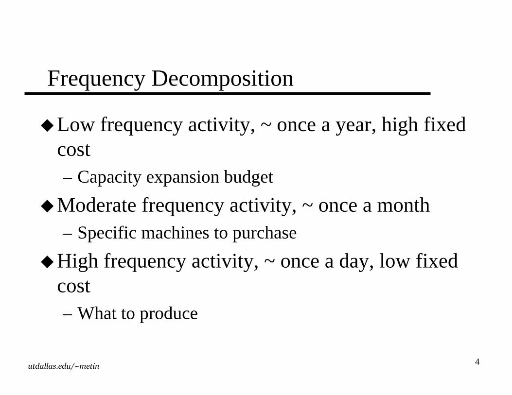
Frequency Decomposition

�Low frequency activity, ~ once a year, high fixed cost– Capacity expansion budget

�Moderate frequency activity, ~ once a month– Specific machines to purchase

�High frequency activity, ~ once a day, low fixed cost– What to produce

5utdallas.edu/~metin

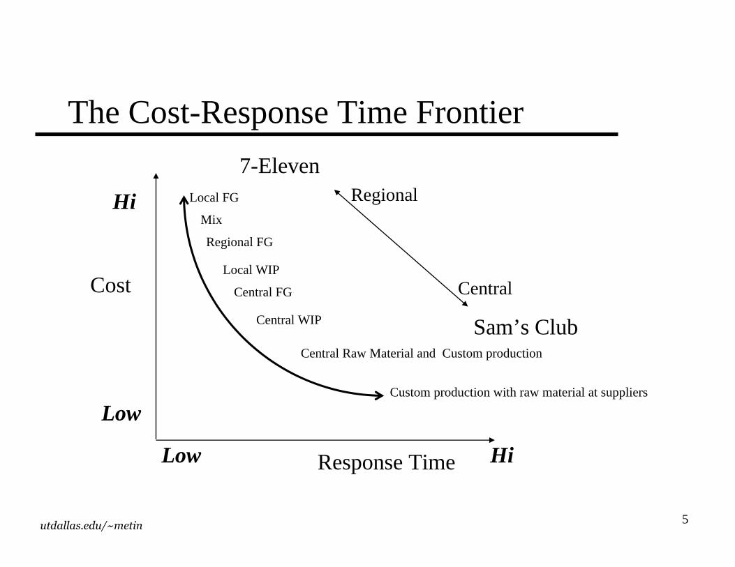
The Cost-Response Time Frontier

Local FG

Mix

Regional FG

Local WIP

Central FG

Central WIP

Central Raw Material and Custom production

Custom production with raw material at suppliers

Cost

Response Time HiLow

Low

Hi

7-Eleven

Sam’s Club

Regional

Central

6utdallas.edu/~metin

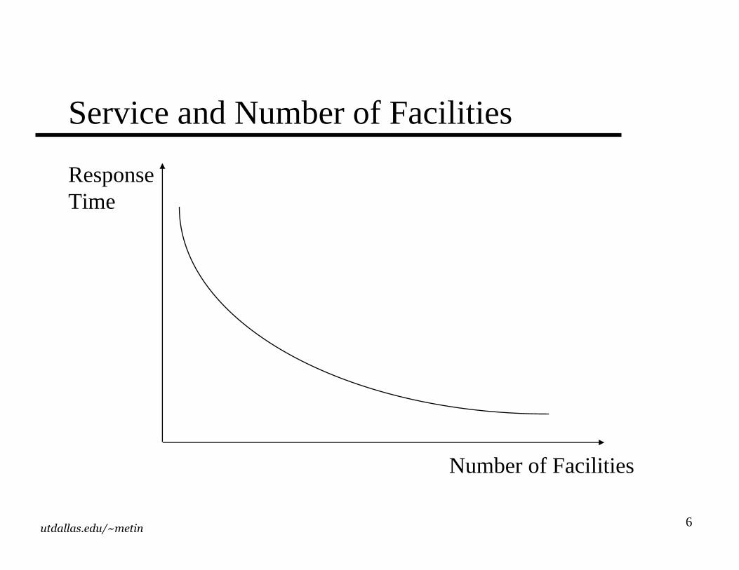
Service and Number of Facilities

Number of Facilities

ResponseTime

7utdallas.edu/~metin

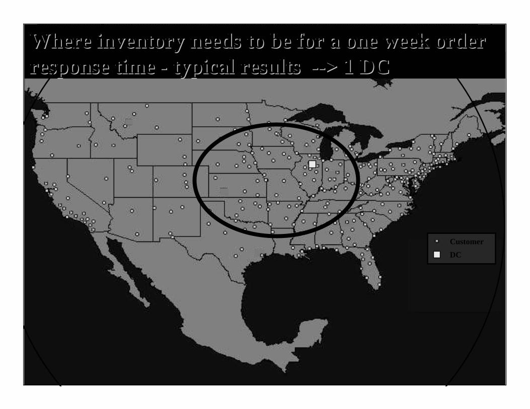
Customer

DC

Where inventory needs to be for a one week order Where inventory needs to be for a one week order response time response time -- typical results typical results ----> 1 DC> 1 DC

8utdallas.edu/~metin

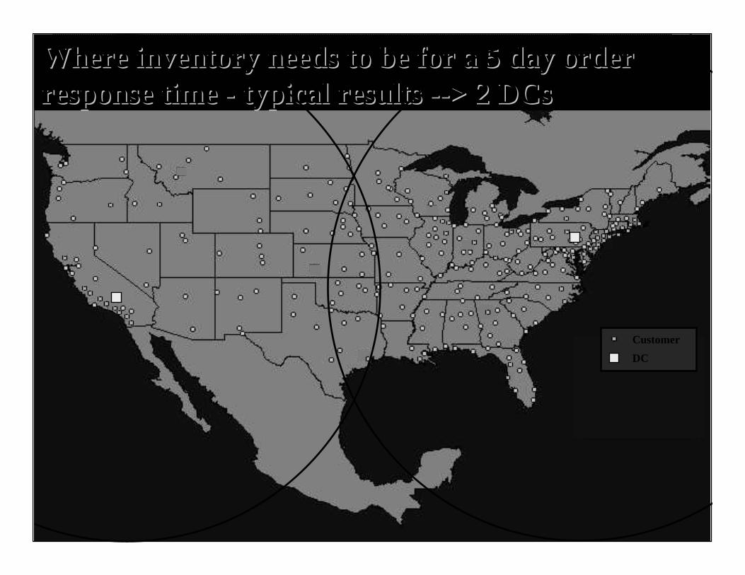
Customer

DC

Where inventory needs to be for a 5 day order Where inventory needs to be for a 5 day order response time response time -- typical results typical results ----> 2 > 2 DCsDCs

9utdallas.edu/~metin

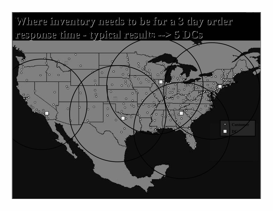
Customer

DC

Where inventory needs to be for a 3 day order Where inventory needs to be for a 3 day order response time response time -- typical results typical results ----> 5 > 5 DCsDCs

10utdallas.edu/~metin

Customer

DC

Where inventory needs to be for a next day order Where inventory needs to be for a next day order response time response time -- typical results typical results ----> 13 > 13 DCsDCs

11utdallas.edu/~metin

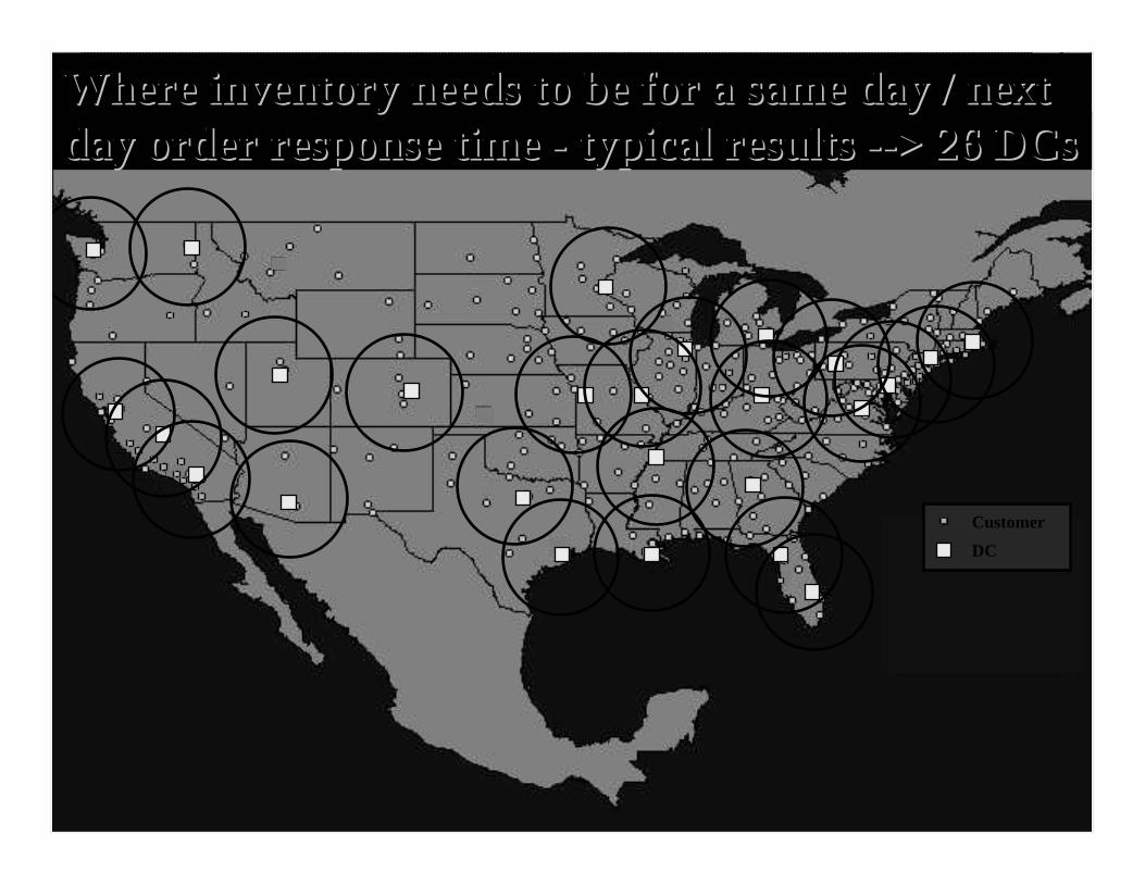
Customer

DC

Where inventory needs to be for a same day / next Where inventory needs to be for a same day / next day order response time day order response time -- typical results typical results ----> 26 > 26 DCsDCs

12utdallas.edu/~metin

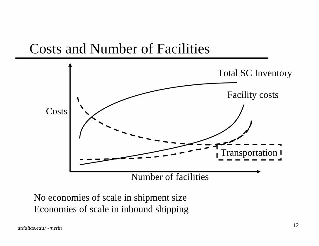
Costs and Number of Facilities

Costs

Number of facilities

Total SC Inventory

Transportation

Facility costs

No economies of scale in shipment sizeEconomies of scale in inbound shipping

13utdallas.edu/~metin

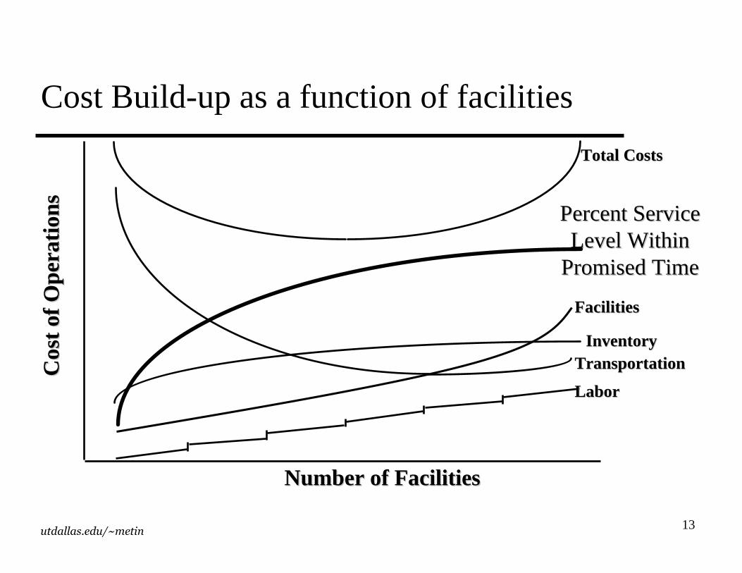
Percent Service Percent Service Level Within Level Within

Promised TimePromised Time

TransportationTransportation

Cost Build-up as a function of facilities

Cos

t of

Ope

rati

ons

Cos

t of

Ope

rati

ons

Number of FacilitiesNumber of Facilities

InventoryInventory

FacilitiesFacilities

Total CostsTotal Costs

LaborLabor

14utdallas.edu/~metin

Network Design Decisions

�Facility function: Plant, DC, Warehouse– Where to locate functions, e.g. packaging

�Facility location

�Capacity allocation

�Market and supply allocation– Who serves whom

15utdallas.edu/~metin

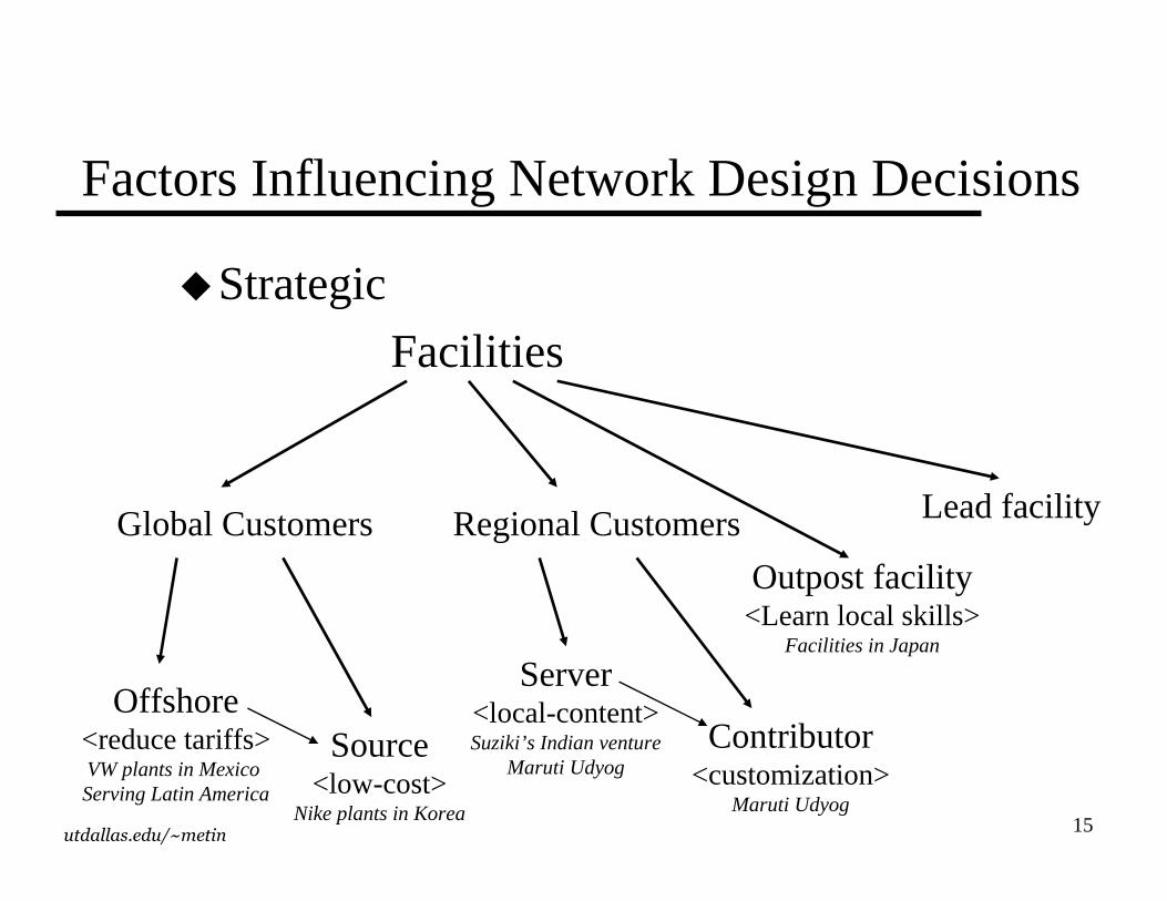
Factors Influencing Network Design Decisions

�Strategic

Facilities

Global Customers

Offshore<reduce tariffs>VW plants in Mexico Serving Latin America

Source<low-cost>

Nike plants in Korea

Regional Customers

Server<local-content>Suziki’s Indian venture

Maruti UdyogContributor

<customization>Maruti Udyog

Lead facility

Outpost facility<Learn local skills>

Facilities in Japan

16utdallas.edu/~metin

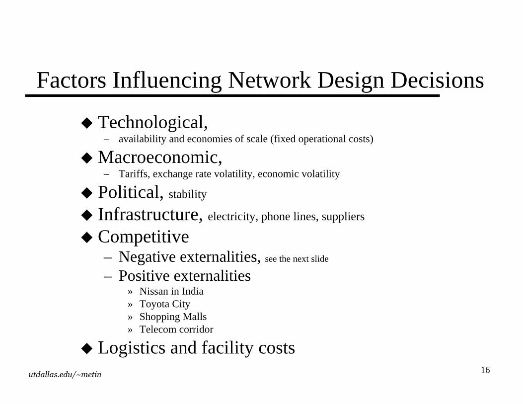
Factors Influencing Network Design Decisions

� Technological, – availability and economies of scale (fixed operational costs)

�Macroeconomic, – Tariffs, exchange rate volatility, economic volatility

� Political, stability

� Infrastructure, electricity, phone lines, suppliers

� Competitive– Negative externalities, see the next slide

– Positive externalities» Nissan in India» Toyota City » Shopping Malls» Telecom corridor

� Logistics and facility costs

17utdallas.edu/~metin

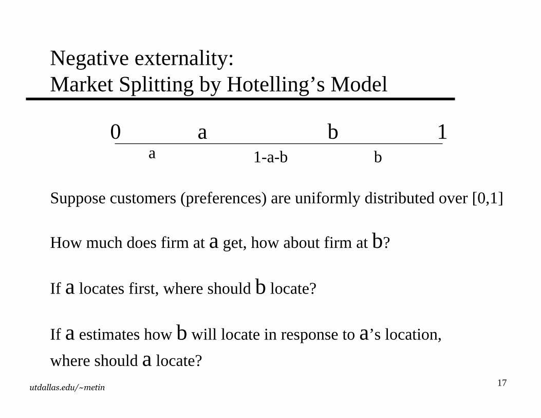
Negative externality:Market Splitting by Hotelling’s Model

0 a b 1a b1-a-b

Suppose customers (preferences) are uniformly distributed over [0,1]

How much does firm at aget, how about firm at b?

If alocates first, where should b locate?

If aestimates how b will locate in response to a’s location,

where should alocate?

18utdallas.edu/~metin

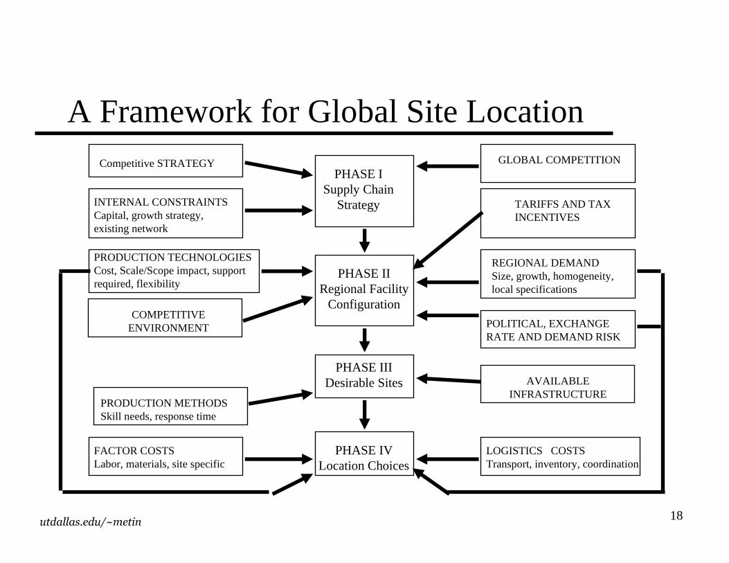
A Framework for Global Site Location

PHASE ISupply Chain

Strategy

PHASE IIRegional Facility

Configuration

PHASE IIIDesirable Sites

PHASE IVLocation Choices

Competitive STRATEGY

INTERNAL CONSTRAINTSCapital, growth strategy,existing network

PRODUCTION TECHNOLOGIESCost, Scale/Scope impact, supportrequired, flexibility

COMPETITIVEENVIRONMENT

PRODUCTION METHODSSkill needs, response time

FACTOR COSTSLabor, materials, site specific

GLOBAL COMPETITION

TARIFFS AND TAXINCENTIVES

REGIONAL DEMANDSize, growth, homogeneity,local specifications

POLITICAL, EXCHANGERATE AND DEMAND RISK

AVAILABLEINFRASTRUCTURE

LOGISTICS COSTSTransport, inventory, coordination

19utdallas.edu/~metin

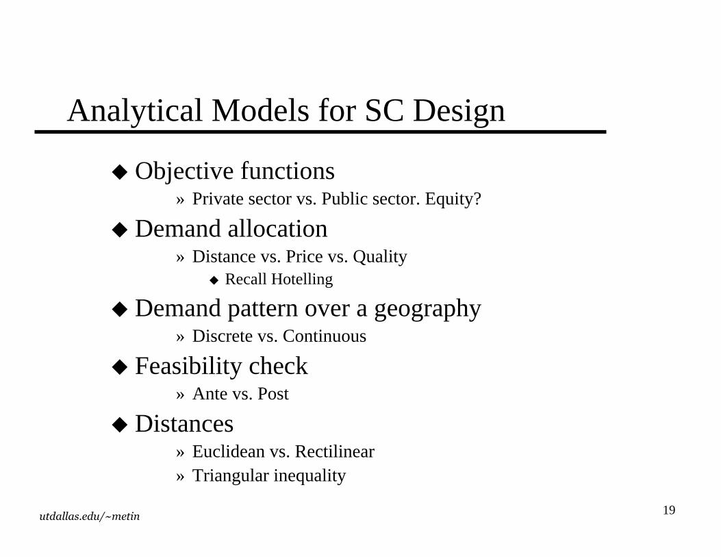
Analytical Models for SC Design

�Objective functions» Private sector vs. Public sector. Equity?

� Demand allocation» Distance vs. Price vs. Quality� Recall Hotelling

� Demand pattern over a geography» Discrete vs. Continuous

� Feasibility check» Ante vs. Post

� Distances» Euclidean vs. Rectilinear» Triangular inequality

20utdallas.edu/~metin

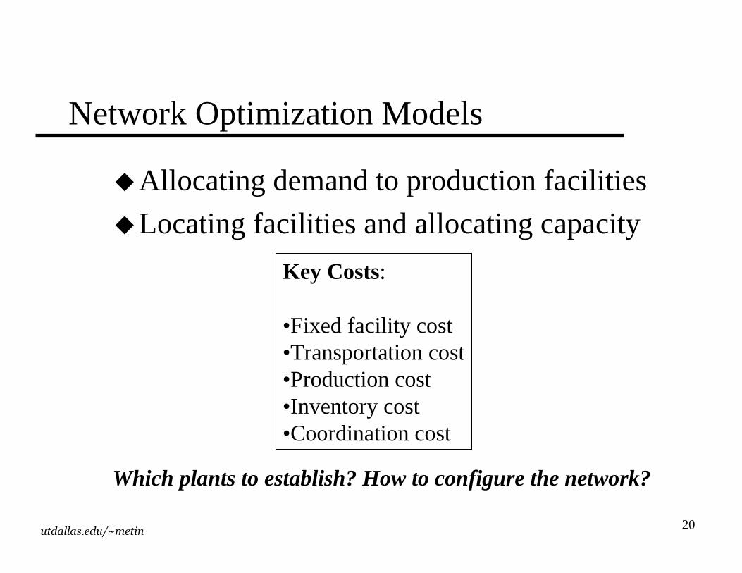
Network Optimization Models

�Allocating demand to production facilities

�Locating facilities and allocating capacity

Which plants to establish? How to configure the network?

Key Costs:

•Fixed facility cost•Transportation cost•Production cost•Inventory cost•Coordination cost

21utdallas.edu/~metin

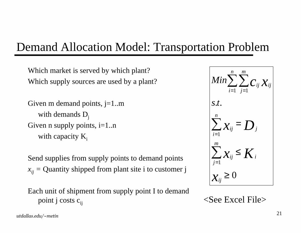
Demand Allocation Model: Transportation Problem

Which market is served by which plant?

Which supply sources are used by a plant?

Given m demand points, j=1..m

with demands Dj

Given n supply points, i=1..n

with capacity Ki

Send supplies from supply points to demand points

xij = Quantity shipped from plant site i to customer j

Each unit of shipment from supply point I to demand point j costs cij

0

..

1

1

1 1

≥

≤

=

∑∑

∑∑

=

=

= =

x

Kx

Dx

xc

ij

i

m

jij

j

n

iij

n

i

m

jijij

ts

Min

<See Excel File>

22utdallas.edu/~metin

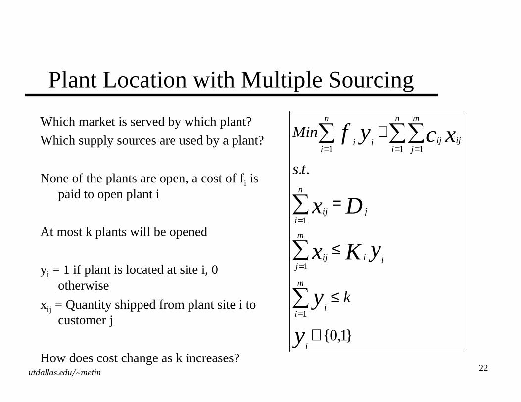
Plant Location with Multiple Sourcing

Which market is served by which plant?

Which supply sources are used by a plant?

None of the plants are open, a cost of fi is paid to open plant i

At most k plants will be opened

yi = 1 if plant is located at site i, 0 otherwise

xij = Quantity shipped from plant site i to customer j

How does cost change as k increases?

}1,0{

..

1

1

1

1 11

∈

≤

≤

=

+

∑∑∑

∑∑∑

=

=

=

= ==

y

y

yKx

Dx

xcyf

i

m

ii

ii

m

jij

j

n

iij

n

i

m

jijiji

n

ii

k

ts

Min

23utdallas.edu/~metin

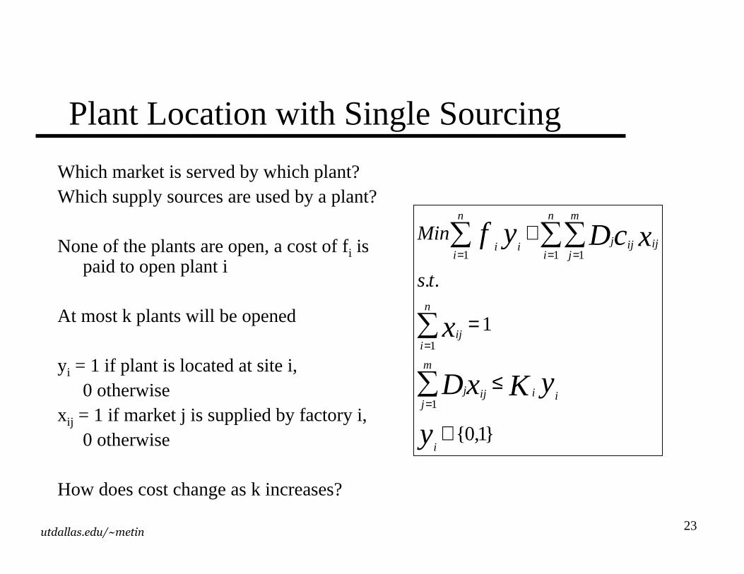
Plant Location with Single Sourcing

Which market is served by which plant?Which supply sources are used by a plant?

None of the plants are open, a cost of fi is paid to open plant i

At most k plants will be opened

yi = 1 if plant is located at site i, 0 otherwise

xij = 1 if market j is supplied by factory i,0 otherwise

How does cost change as k increases?

}1,0{

1

..

1

1

1 11

∈

≤

=

+

∑∑

∑∑∑

=

=

= ==

y

yKxD

x

xcDyf

i

ii

m

jj ij

n

iij

n

i

m

jijj iji

n

ii

ts

Min

24utdallas.edu/~metin

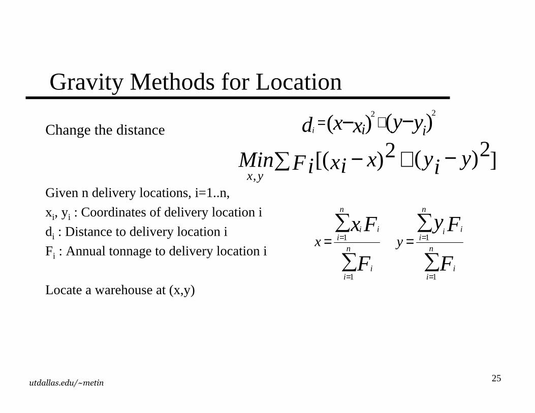
Gravity Methods for Location

Ton Mile-Center SolutionGiven n delivery locations, i=1..n,

xi, yi : Coordinates of delivery location i

di : Distance to delivery location i

Fi : Annual tonnage to delivery location i

Locate a warehouse at (x,y)

∑ −+−=

n

iyyxxF iii1

yx, )()( 22Min

<Show Excel File> ∑∑

∑∑

=

=

=

= ==n

i i

i

n

i i

ii

n

i i

i

n

i i

ii

d

Fd

Fy

y

d

Fd

Fx

x

1

1

1

1

)()(22

yyxxd iii −− +=

25utdallas.edu/~metin

Gravity Methods for Location

∑∑

∑∑

=

=

=

= ==n

ii

n

iii

n

ii

n

iii

F

Fy

F

Fxyx

1

1

1

1

∑ −+− ])( 2)( 2[,

yyixxiFiMinyx

Change the distance

Given n delivery locations, i=1..n,

xi, yi : Coordinates of delivery location i

di : Distance to delivery location i

Fi : Annual tonnage to delivery location i

Locate a warehouse at (x,y)

)()(22

yyxxd iii −− +=

26utdallas.edu/~metin

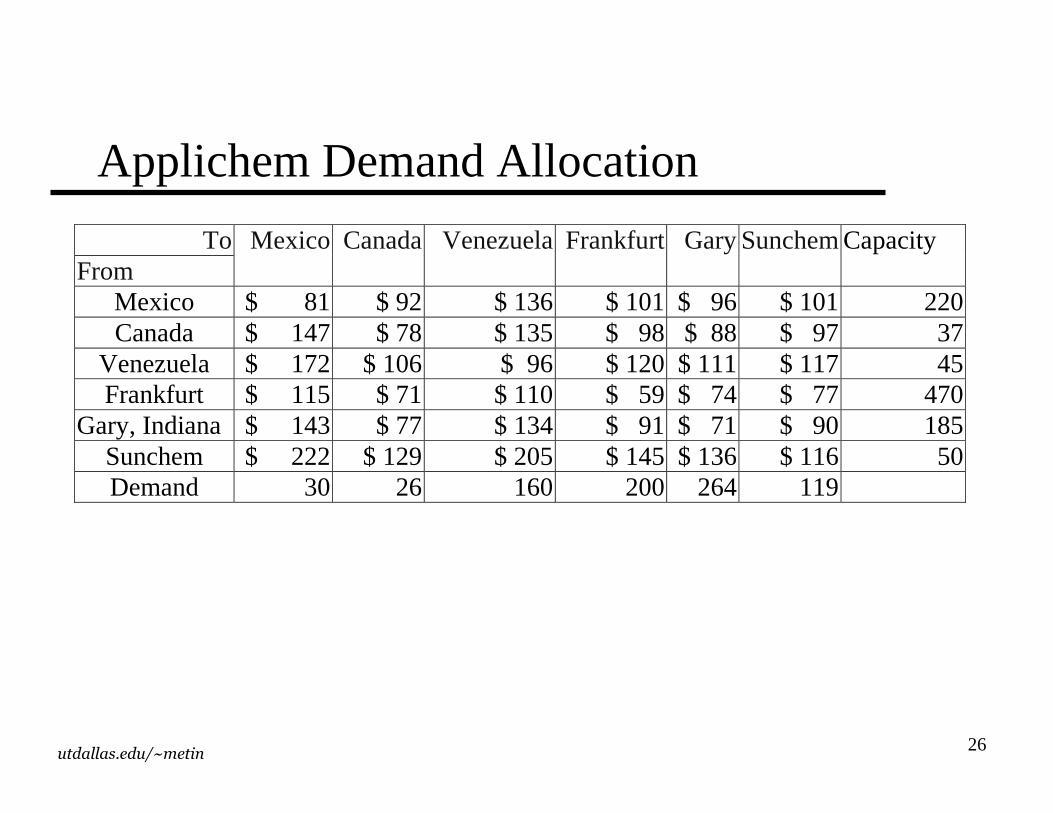
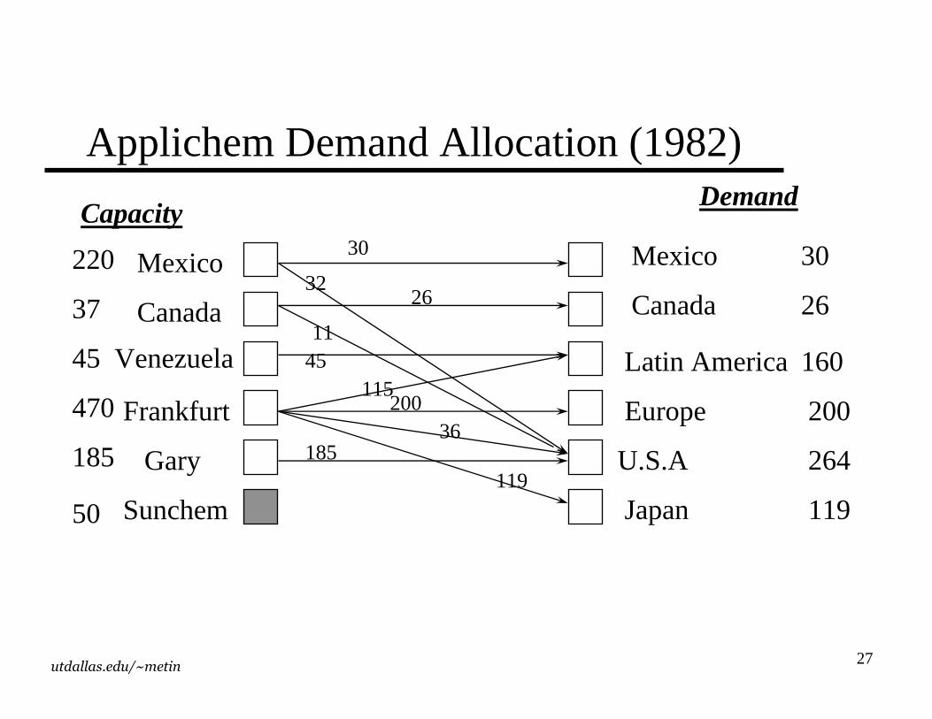
Applichem Demand Allocation

To From

Mexico Canada Venezuela Frankfurt Gary Sunchem Capacity

Mexico $ 81 $ 92 $ 136 $ 101 $ 96 $ 101 220 Canada $ 147 $ 78 $ 135 $ 98 $ 88 $ 97 37

Venezuela $ 172 $ 106 $ 96 $ 120 $ 111 $ 117 45 Frankfurt $ 115 $ 71 $ 110 $ 59 $ 74 $ 77 470

Gary, Indiana $ 143 $ 77 $ 134 $ 91 $ 71 $ 90 185 Sunchem $ 222 $ 129 $ 205 $ 145 $ 136 $ 116 50 Demand 30 26 160 200 264 119

27utdallas.edu/~metin

Applichem Demand Allocation (1982)Demand

Mexico

Canada

Frankfurt

Gary

Sunchem

Mexico 30

Canada 26

Latin America 160

Europe 200

U.S.A 264

Japan 119

30

3226

11Venezuela

220

Capacity

37

45

470

185

50

45115

20036

119185

28utdallas.edu/~metin

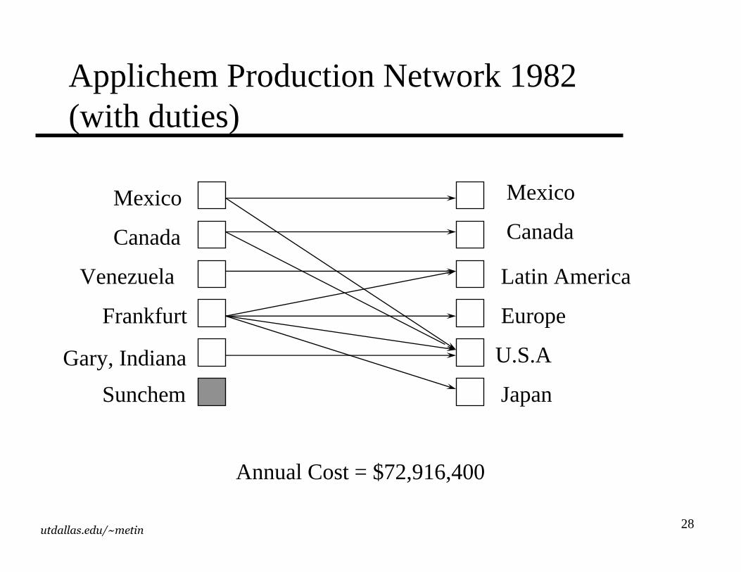
Applichem Production Network 1982 (with duties)

Venezuela

Annual Cost = $72,916,400

Mexico

Canada

Frankfurt

Sunchem

Mexico

Canada

Latin America

Europe

U.S.A

Japan

Gary, Indiana

29utdallas.edu/~metin

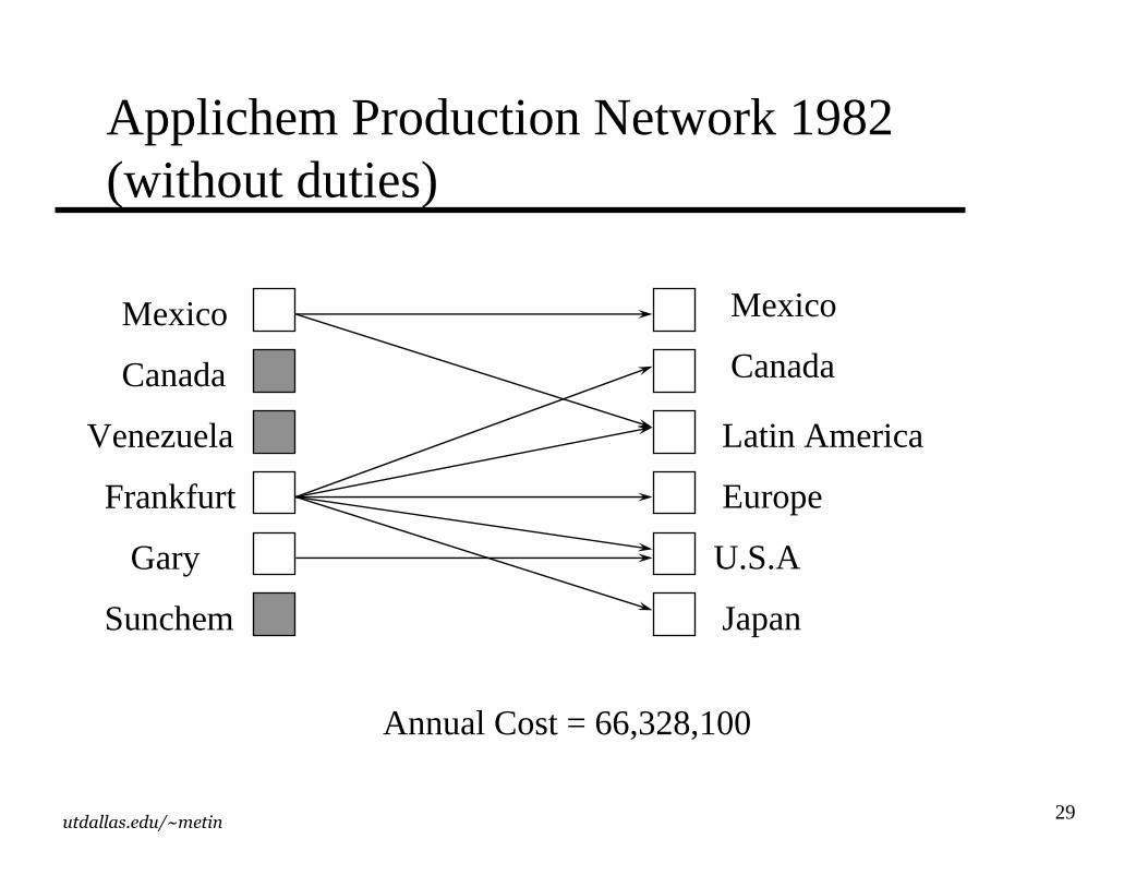
Applichem Production Network 1982 (without duties)

Mexico

Canada

Venezuela

Frankfurt

Gary

Sunchem

Mexico

Canada

Latin America

Europe

U.S.A

Japan

Annual Cost = 66,328,100

30utdallas.edu/~metin

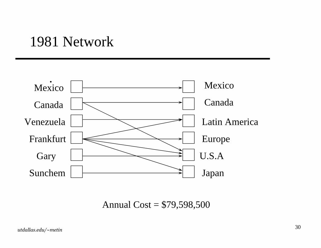
1981 Network

.Mexico

Canada

Venezuela

Frankfurt

Gary

Sunchem

Mexico

Canada

Latin America

Europe

U.S.A

Japan

Annual Cost = $79,598,500

31utdallas.edu/~metin

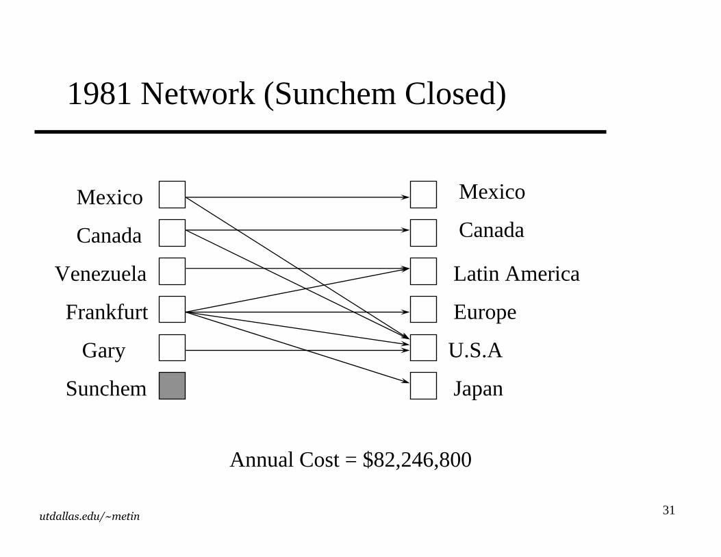
1981 Network (Sunchem Closed)

Mexico

Canada

Venezuela

Frankfurt

Gary

Sunchem

Mexico

Canada

Latin America

Europe

U.S.A

Japan

Annual Cost = $82,246,800

32utdallas.edu/~metin

Cash Flows From Sunchem Plant

Year 1977 1978 1979 1980 1981 1982

Optimal($ Million)

60.562 68.889 75.999 79.887 79.598 72.916

SunchemClosed

60.721 68.889 77.503 80.999 82.247 72.916

Difference 0.159 0.000 1.504 1.112 2.649 0.000

33utdallas.edu/~metin

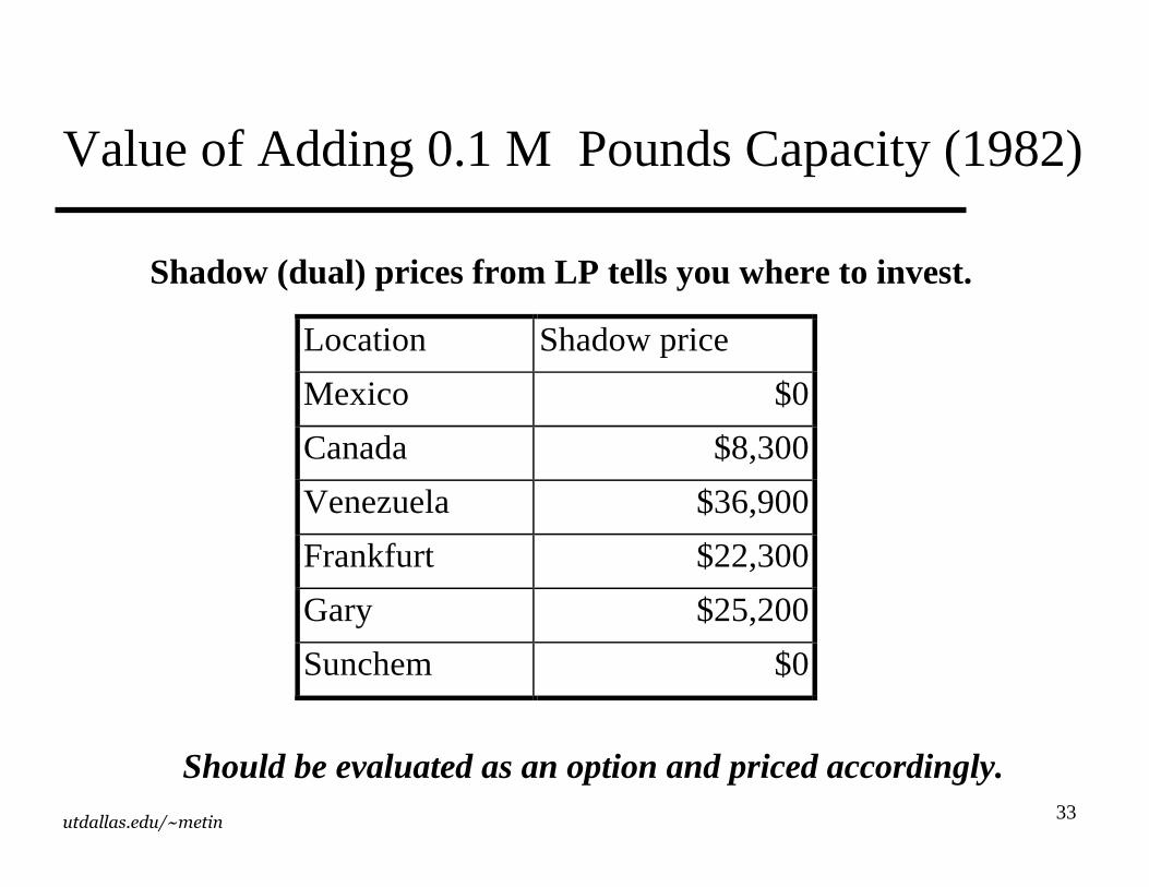
Value of Adding 0.1 M Pounds Capacity (1982)

Location Shadow price

Mexico $0

Canada $8,300

Venezuela $36,900

Frankfurt $22,300

Gary $25,200

Sunchem $0

Should be evaluated as an option and priced accordingly.

Shadow (dual) prices from LP tells you where to invest.

34utdallas.edu/~metin

Chapter 6

Network Design in an Uncertain Environment

35utdallas.edu/~metin

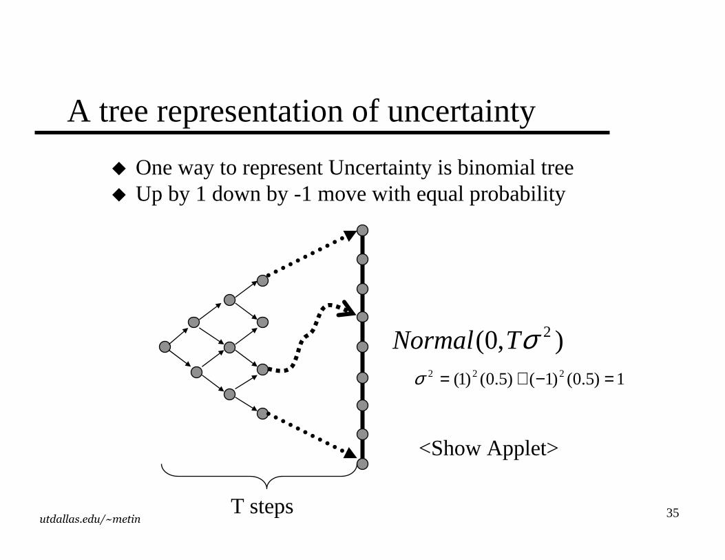
A tree representation of uncertainty

� One way to represent Uncertainty is binomial tree� Up by 1 down by -1 move with equal probability

),0( 2σTNormal

T steps

1)5.0()1()5.0()1( 222 =−+=σ

<Show Applet>

36utdallas.edu/~metin

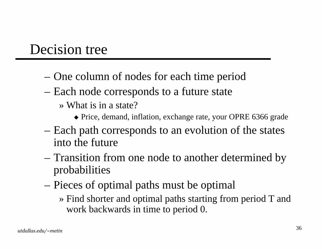
Decision tree

– One column of nodes for each time period– Each node corresponds to a future state

» What is in a state?� Price, demand, inflation, exchange rate, your OPRE 6366 grade

– Each path corresponds to an evolution of the states into the future

– Transition from one node to another determined by probabilities

– Pieces of optimal paths must be optimal» Find shorter and optimal paths starting from period T and

work backwards in time to period 0.

37utdallas.edu/~metin

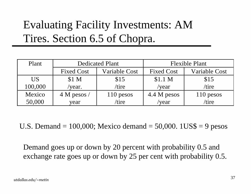
Evaluating Facility Investments: AM Tires. Section 6.5 of Chopra.

Dedicated Plant Flexible Plant Plant Fixed Cost Variable Cost Fixed Cost Variable Cost

US 100,000

$1 M /year.

$15 /tire

$1.1 M /year

$15 /tire

Mexico 50,000

4 M pesos / year

110 pesos /tire

4.4 M pesos /year

110 pesos /tire

U.S. Demand = 100,000; Mexico demand = 50,000. 1US$ = 9 pesos

Demand goes up or down by 20 percent with probability 0.5 andexchange rate goes up or down by 25 per cent with probability 0.5.

38utdallas.edu/~metin

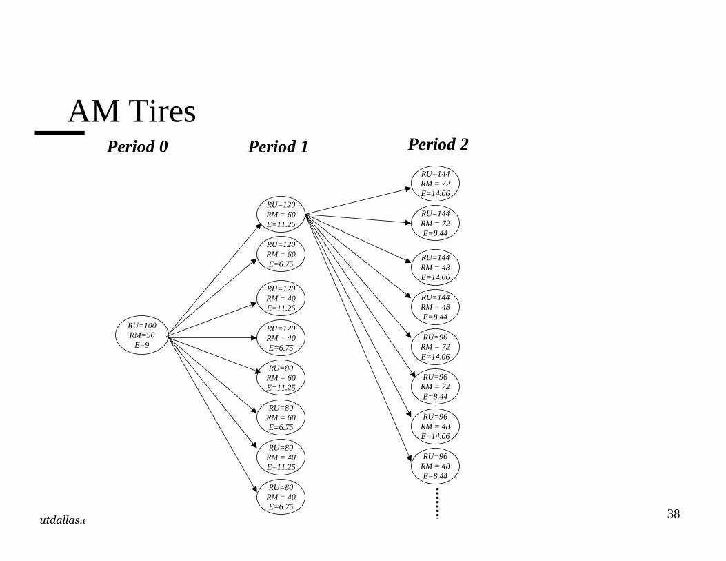
AM Tires

RU=100RM=50

E=9

Period 0 Period 1 Period 2

RU=120RM = 60E=11.25

RU=120RM = 60E=6.75

RU=120RM = 40E=11.25

RU=120RM = 40E=6.75

RU=80RM = 60E=11.25

RU=80RM = 60E=6.75

RU=80RM = 40E=11.25

RU=80RM = 40E=6.75

RU=144RM = 72E=14.06

RU=144RM = 72E=8.44

RU=144RM = 48E=14.06

RU=144RM = 48E=8.44

RU=96RM = 72E=14.06

RU=96RM = 72E=8.44

RU=96RM = 48E=14.06

RU=96RM = 48E=8.44

39utdallas.edu/~metin

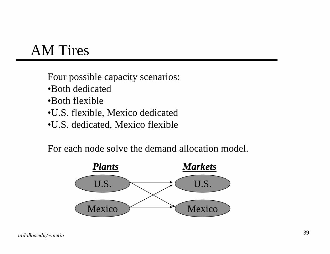
AM Tires

Four possible capacity scenarios:•Both dedicated•Both flexible•U.S. flexible, Mexico dedicated•U.S. dedicated, Mexico flexible

For each node solve the demand allocation model.

Plants Markets

U.S.

Mexico

U.S.

Mexico

40utdallas.edu/~metin

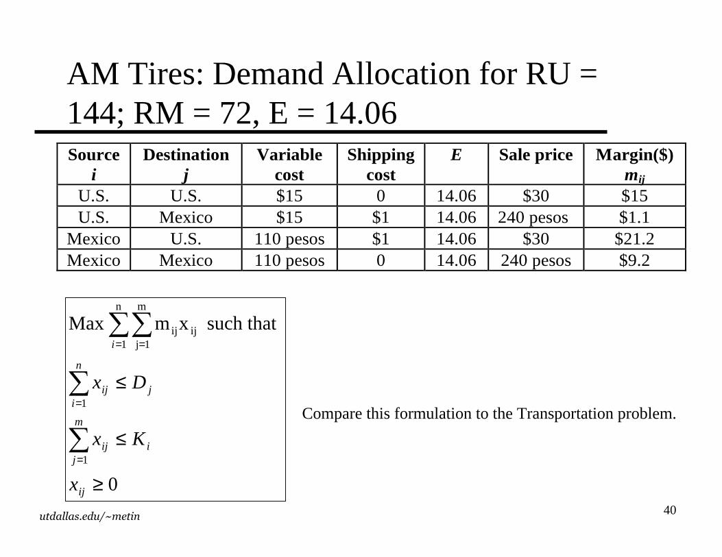
AM Tires: Demand Allocation for RU = 144; RM = 72, E = 14.06Source

i Destination

j Variable

cost Shipping

cost E Sale price Margin($)

mij

U.S. U.S. $15 0 14.06 $30 $15 U.S. Mexico $15 $1 14.06 240 pesos $1.1

Mexico U.S. 110 pesos $1 14.06 $30 $21.2 Mexico Mexico 110 pesos 0 14.06 240 pesos $9.2

0

such that xmMax

1

1

n

1

m

1jijij

≥

≤

≤

∑∑∑∑

=

=

= =

ij

i

m

jij

j

n

iij

i

x

Kx

Dx

Compare this formulation to the Transportation problem.

41utdallas.edu/~metin

AM Tires: Demand Allocation for RU = 144; RM = 72, E = 14.06

Plants Markets

U.S.

Mexico

U.S.

Mexico

100,000

44,000

6,000

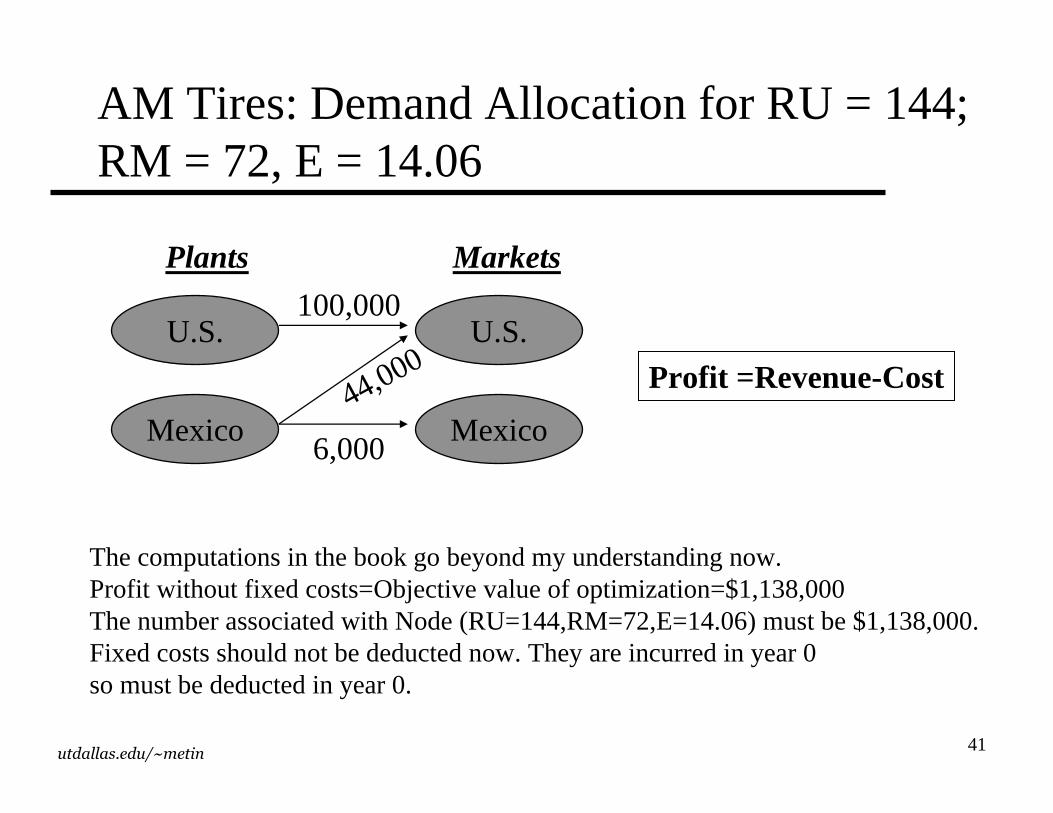
Profit =Revenue-Cost

The computations in the book go beyond my understanding now.Profit without fixed costs=Objective value of optimization=$1,138,000The number associated with Node (RU=144,RM=72,E=14.06) must be $1,138,000.Fixed costs should not be deducted now. They are incurred in year 0so must be deducted in year 0.

42utdallas.edu/~metin

Facility Decision at AM Tires

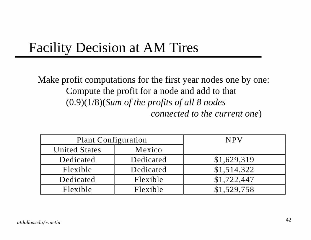
Plant ConfigurationUnited States M exico

NPV

Dedicated Dedicated $1,629,319Flexible Dedicated $1,514,322

Dedicated Flexible $1,722,447Flexible Flexible $1,529,758

Make profit computations for the first year nodes one by one:Compute the profit for a node and add to that(0.9)(1/8)(Sum of the profits of all 8 nodes

connected to the current one)

43utdallas.edu/~metin

Capacity Investment Strategies

� Single sourcing� Hedging Strategy

– Risk management? – Match revenue and cost exposure

� Flexible Strategy– Excess total capacity in multiple plants– Flexible technologies

�More will be said in aggregate planning chapter

44utdallas.edu/~metin

Summary

�Frequency decomposition

�Factors influencing facility decisions

�A strategic framework for facility location

�Gravity methods for location

�Network-LP-IP optimization models

�Value capacity as a real option

45utdallas.edu/~metin

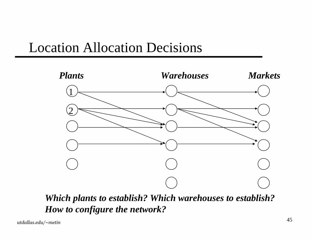
Location Allocation Decisions

Plants Warehouses

1

2

Which plants to establish? Which warehouses to establish?How to configure the network?

Markets

46utdallas.edu/~metin

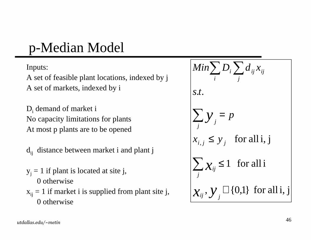
p-Median ModelInputs: A set of feasible plant locations, indexed by jA set of markets, indexed by i

Di demand of market iNo capacity limitations for plants At most p plants are to be opened

dij distance between market i and plant j

yj = 1 if plant is located at site j, 0 otherwise

xij = 1 if market i is supplied from plant site j, 0 otherwise

ji, allfor }1,0{,

i allfor 1

ji, allfor

..

,

∈

≤

≤

=

∑

∑

∑∑

yx

x

y

jij

jij

jji

jj

jijij

ii

yx

p

ts

xdDMin

47utdallas.edu/~metin

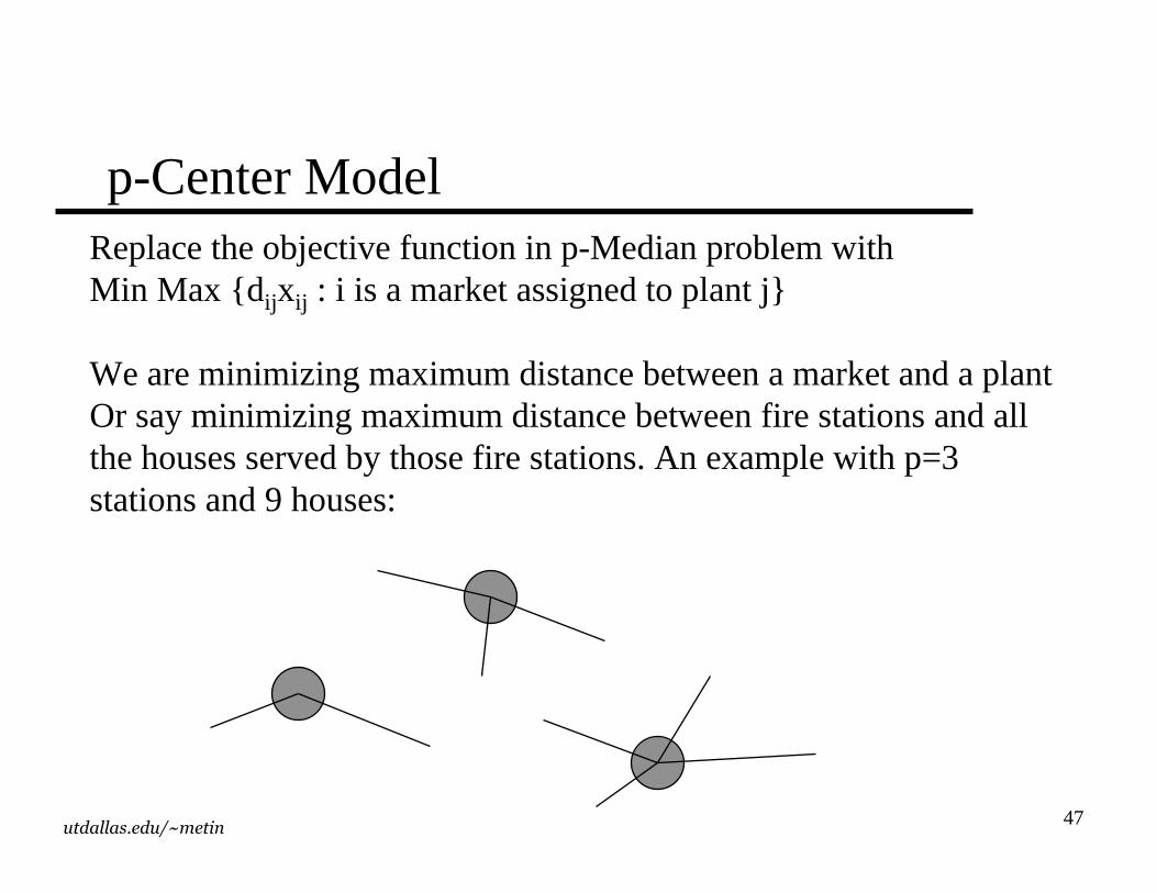
p-Center ModelReplace the objective function in p-Median problem withMin Max { dijxij : i is a market assigned to plant j}

We are minimizing maximum distance between a market and a plantOr say minimizing maximum distance between fire stations and allthe houses served by those fire stations. An example with p=3 stations and 9 houses:

48utdallas.edu/~metin

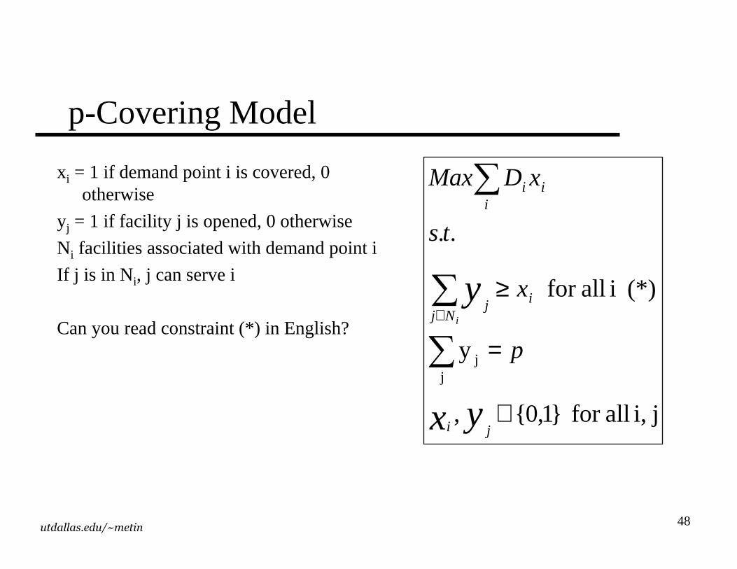
p-Covering Model

xi = 1 if demand point i is covered, 0 otherwise

yj = 1 if facility j is opened, 0 otherwise

Ni facilities associated with demand point i

If j is in Ni, j can serve i

Can you read constraint (* ) in English?

ji, allfor }1,0{,

y

(* ) i allfor

..

jj

∈

=

≥

∑∑

∑

∈

yx

y

ji

iNj

j

ii

i

p

x

ts

xDMax

i

49utdallas.edu/~metin

Other Models

�p-Choice Models– Criteria to choose the server: distance, price?

�Models with multiple decision makers– Franchise model