Safety Inventories - The University of Texas at Dallasmetin/FuJen/Folios/scstocinventory_s.pdf · Safety Inventories Chapter 11 of Chopra. ... If Safety inventory is up, ... Buying

1utdallas.edu/~metin

Safety Inventories

Chapter 11 of Chopra


Why to hold Safety Inventory?

� Desire for product availability– Ease of search for another supplier

– “ I want it now” culture

� Demand uncertainty – Short product life cycles

� Safety inventory


Measures

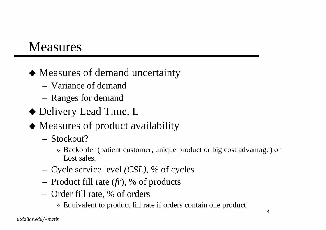
�Measures of demand uncertainty– Variance of demand– Ranges for demand

� Delivery Lead Time, L�Measures of product availability

– Stockout? » Backorder (patient customer, unique product or big cost advantage) or

Lost sales.

– Cycle service level (CSL), % of cycles– Product fill rate (fr), % of products– Order fill rate, % of orders

» Equivalent to product fill rate if orders contain one product


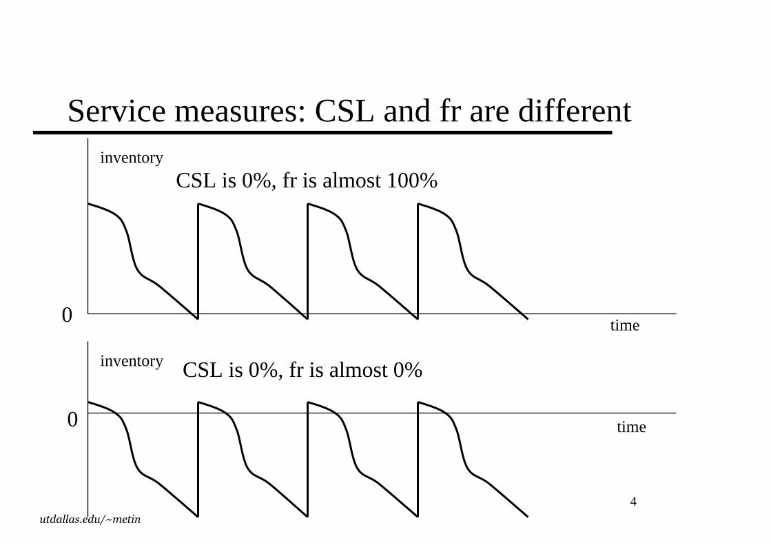
Service measures: CSL and fr are different

CSL is 0%, fr is almost 100%

CSL is 0%, fr is almost 0%

inventory

inventory

time

time

0

0


Replenishment policies

�When to reorder?� How much to reorder?

– Most often these decisions are related.

Continuous Review: Order fixed quantity when total inventory drops below Reorder Point (ROP).

ROP meets the demand during the lead time L.One has to figure out the ROP.Information technology facilitates continuous review.


Demand During Lead time

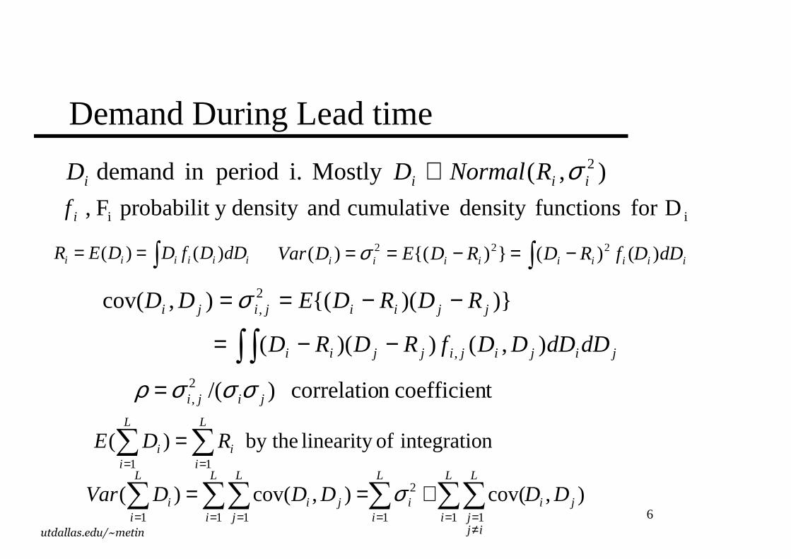
),(Mostly i. periodin demand 2iiii RNormalDD σ∝

∫ ∫ −−=

−−==

jijijijjii

jjiijiji

dDdDDDfRDRD

RDRDEDD

),())((

)})({ (),cov(

,

2,σ

∫== iiiiii dDDfDDER )()(

Dfor functionsdensity cumulative anddensity y probabilit F , iiif

iiiiiiiii dDDfRDRDEDVar )()(}){ ()( 222 ∫ −=−== σ

nintegratio oflinearity by the )(11∑∑

==

=L

ii

L

ii RDE

),cov(),cov()(1 11

2

1 11ji

L

i

L

ijj

L

ii

L

i

L

jji

L

ii DDDDDVar ∑∑∑∑∑∑

=≠=== ==

+== σ

tcoefficienn correlatio )/(2, jiji σσσρ =


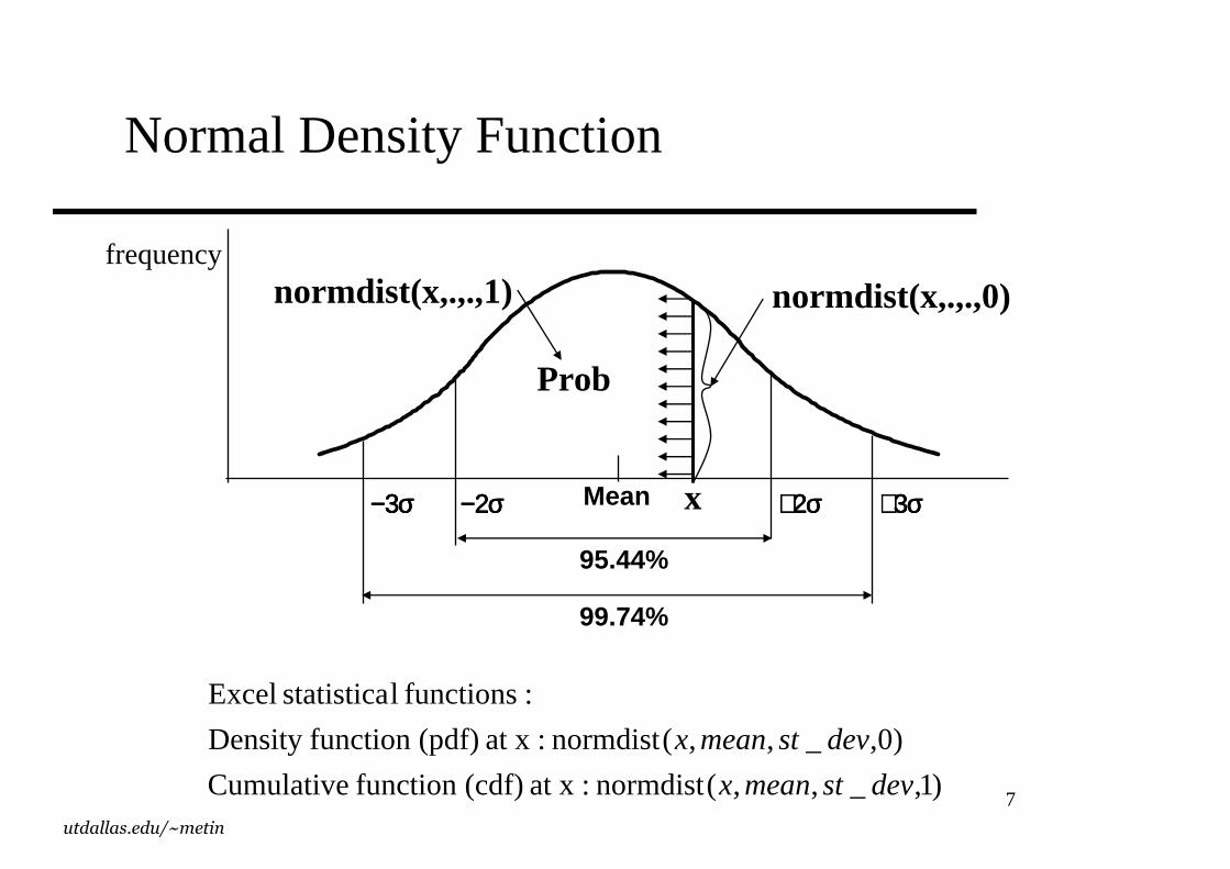
Normal Density Function

Mean−−−−3333σσσσ −−−−2222σσσσ ++++2222σσσσ ++++3333σσσσ

95.44%

99.74%

x

)1,_,,(normdist:at x (cdf)function Cumulative

)0,_,,(normdist:at x (pdf)function Density

:functions lstatistica Excel

devstmeanx

devstmeanx

normdist(x,.,.,0)

Prob

normdist(x,.,.,1)frequency


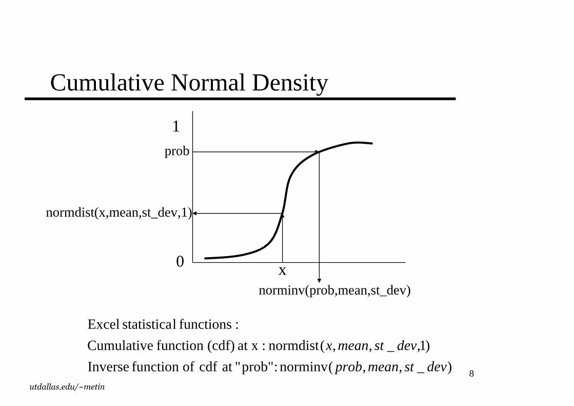
Cumulative Normal Density

)_,,(norminv :prob""at cdf offunction Inverse

)1,_,,(normdist:at x (cdf)function Cumulative

:functions lstatistica Excel

devstmeanprob

devstmeanx

0

1

x

normdist(x,mean,st_dev,1)

prob

norminv(prob,mean,st_dev)


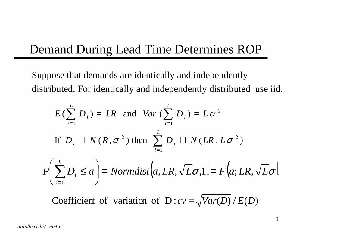
Demand During Lead Time Determines ROP

Suppose that demands are identically and independently

distributed. For identically and independently distributed use iid.

),( then ),( If

)( and )(

2

1

2

2

11

σσ

σ

LLRNDRND

LDVarLRDE

L

iii

L

ii

L

ii

∝∝

==

∑∑∑

=

==

( ) ( )σσ LLRaFLLRaNormdistaDPL

ii ,;1,,,

1

==

≤∑=

)(/)( :D ofn variatiooft Coefficien DEDVarcv =


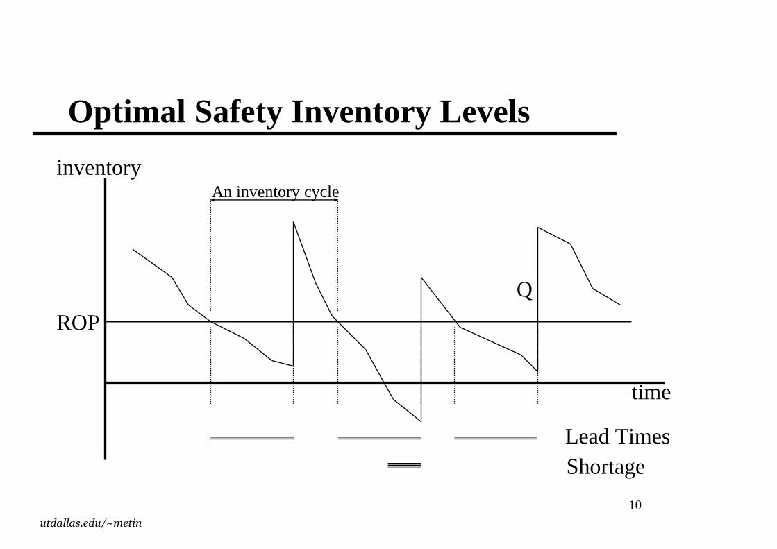
Optimal Safety Inventory Levels

Lead Times

time

inventory

Shortage

An inventory cycle

ROP

Q


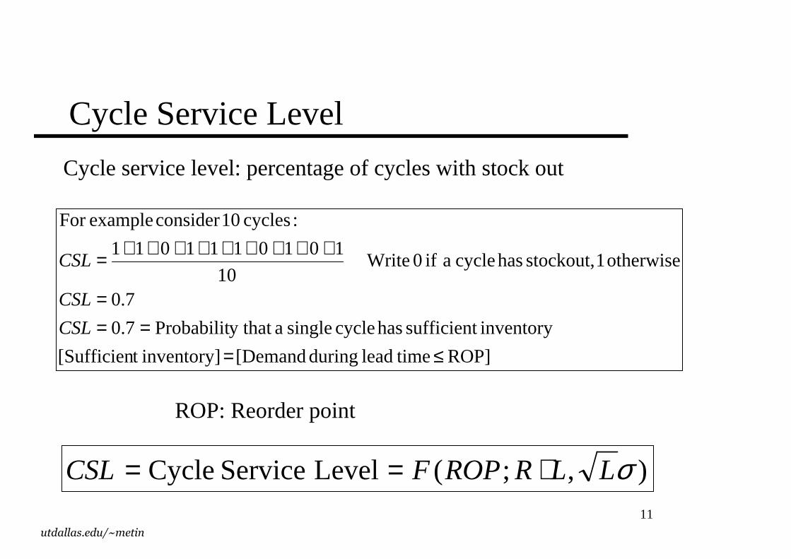
Cycle Service Level

),;(Level Service Cycle σLLRROPFCSL ⋅==

Cycle service level: percentage of cycles with stock out

ROP] timelead during [Demand inventory]t [Sufficien

inventory sufficient has cycle single ay that Probabilit0.7

7.0

otherwise 1 stockout, has cycle a if 0 Write10

1010111011

:cycles 10consider exampleFor

≤===

=

+++++++++=

CSL

CSL

CSL

ROP: Reorder point


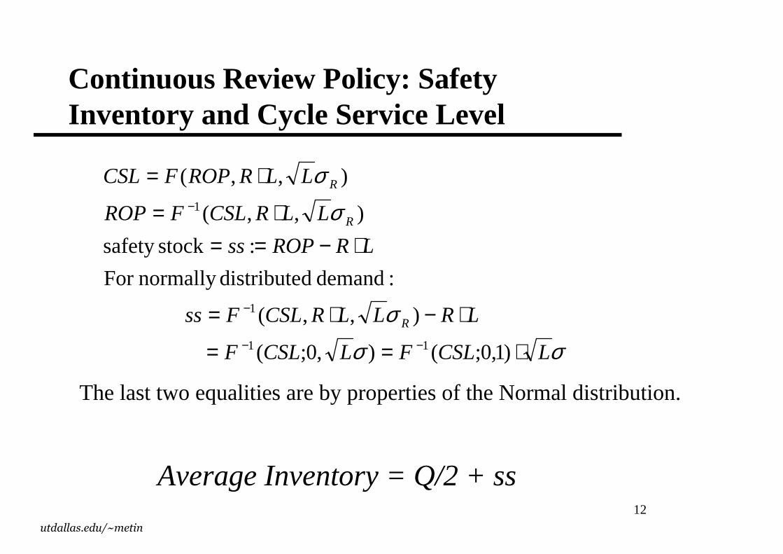
Continuous Review Policy: Safety Inventory and Cycle Service Level

σσ

σ

σ

σ

LCSLFLCSLF

LRLLRCSLFss

LRROPss

LLRCSLFROP

LLRROPFCSL

R

R

R

⋅==

⋅−⋅=

⋅−==⋅=

⋅=

−−

−

−

)1,0;(),0;(

),,(

:demand ddistributenormally For

:stocksafety

),,(

),,(

11

1

1

Average Inventory = Q/2 + ss

The last two equalities are by properties of the Normal distribution.


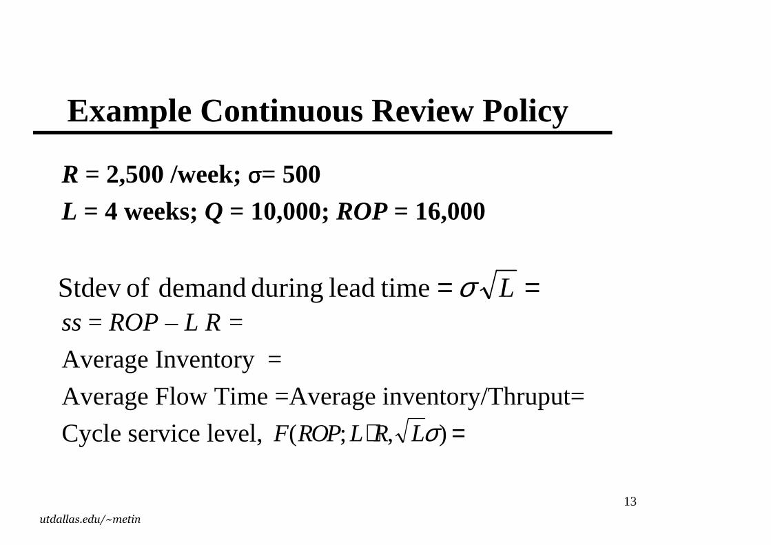
Example Continuous Review Policy

R = 2,500 /week; σσσσ= 500

L = 4 weeks; Q = 10,000; ROP = 16,000

ss= ROP – L R =

Average Inventory =

Average Flow Time =Average inventory/Thruput=

Cycle service level,

== Lσ timelead during demand of Stdev

F ROP L R L( ; , )⋅ =σ


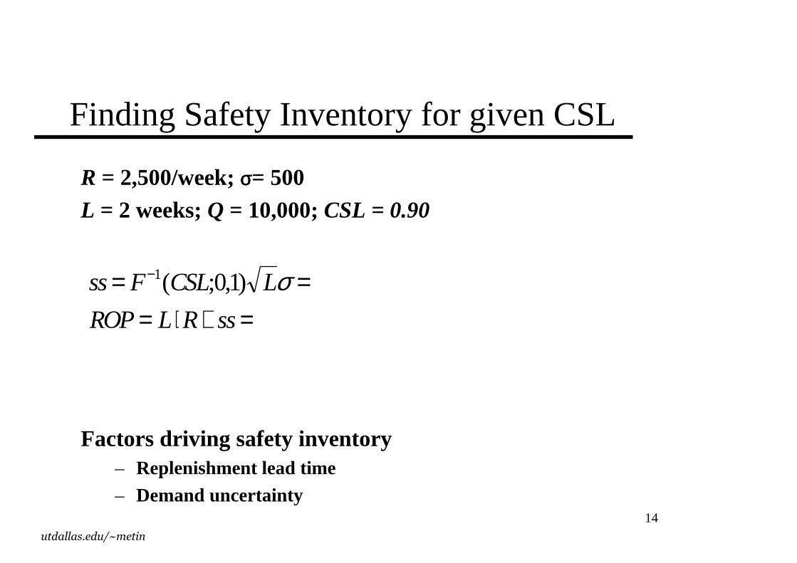
Finding Safety Inventory for given CSL

R = 2,500/week; σσσσ= 500L = 2 weeks; Q = 10,000; CSL = 0.90

Factors dr iving safety inventory– Replenishment lead time– Demand uncer tainty

ss F CSL L

ROP L R ss

= == ⋅ + =

−1 01( ; , ) σ


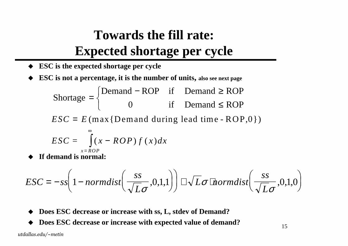
Towards the fill rate:Expected shor tage per cycle

� ESC is the expected shor tage per cycle

� ESC is not a percentage, it is the number of units, also see next page

� I f demand is normal:

� Does ESC decrease or increase with ss, L , stdev of Demand?

� Does ESC decrease or increase with expected value of demand?

ESC E

ESC x ROP f x dxx ROP

=

−=

∞∫(max{

( ) ( )

Demand during lead time - ROP,0} )

=

ESC ss normdistss

LL normdist

ss

L= − −

+ ⋅

1 011 010

σσ

σ, , , , , ,

≤≥−

=ROPDemand

ROPDemand

if

if

0

ROPDemandShortage


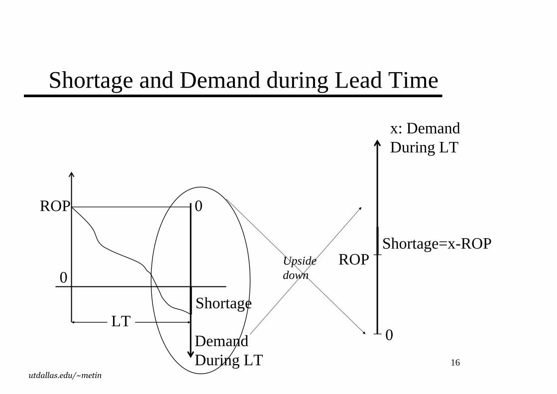
Shortage and Demand during Lead Time

0

ROP

Demand During LT

LTShortage

x: Demand During LT

0

0

ROPShortage=x-ROP

Upsidedown


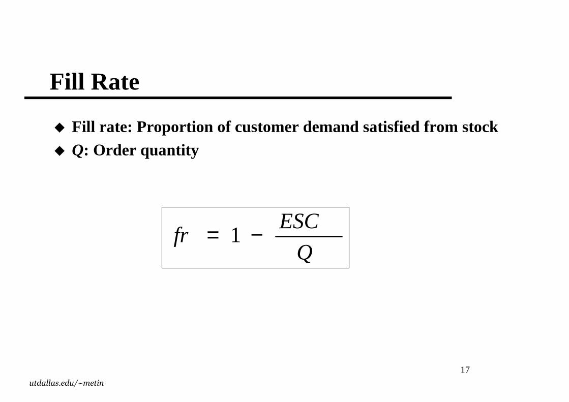
Fill Rate

� Fill rate: Propor tion of customer demand satisfied from stock� Q: Order quantity

Q

ESCfr −= 1


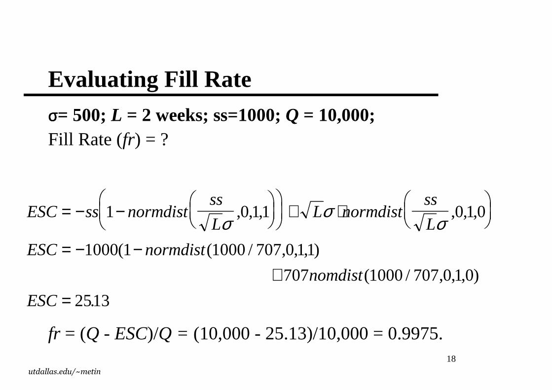
Evaluating Fill Rate

σσσσ= 500; L = 2 weeks; ss=1000; Q = 10,000; Fill Rate (fr) = ?

fr = (Q - ESC)/Q = (10,000 - 25.13)/10,000 = 0.9975.

ESC ss normdistss

LL normdist

ss

L

ESC normdist

nomdist

ESC

= − −

+ ⋅

= − −+

=

1 011 010

1000 1 1000 707 011

707 1000 707 010

2513

σσ

σ, , , , , ,

( ( / , , , )

( / , , , )

.


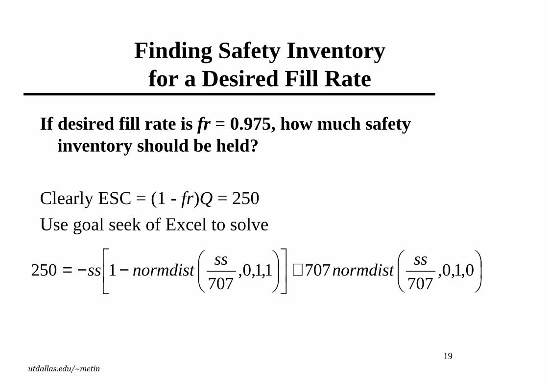
Finding Safety Inventory for a Desired Fill Rate

I f desired fill rate is fr = 0.975, how much safety inventory should be held?

Clearly ESC = (1 - fr)Q = 250

Use goal seek of Excel to solve

+

−−= 0,1,0,707

7071,1,0,707

1250ss

normdistss

normdistss


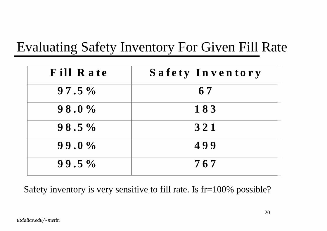
Evaluating Safety Inventory For Given Fill Rate

F i l l R a t e Sa f et y I n v en t o r y

9 7 .5 % 6 7

9 8 .0 % 1 8 3

9 8 .5 % 3 2 1

9 9 .0 % 4 9 9

9 9 .5 % 7 6 7

Safety inventory is very sensitive to fill rate. Is fr=100% possible?


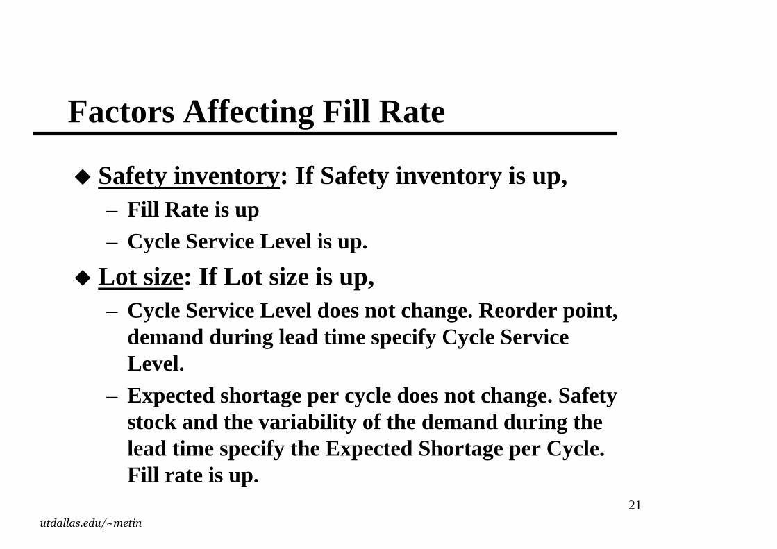
Factors Affecting Fill Rate

� Safety inventory: I f Safety inventory is up, – Fill Rate is up – Cycle Service Level is up.

� Lot size: I f Lot size is up, – Cycle Service Level does not change. Reorder point,

demand dur ing lead time specify Cycle Service Level.

– Expected shor tage per cycle does not change. Safety stock and the var iability of the demand dur ing the lead time specify the Expected Shor tage per Cycle. Fill rate is up.


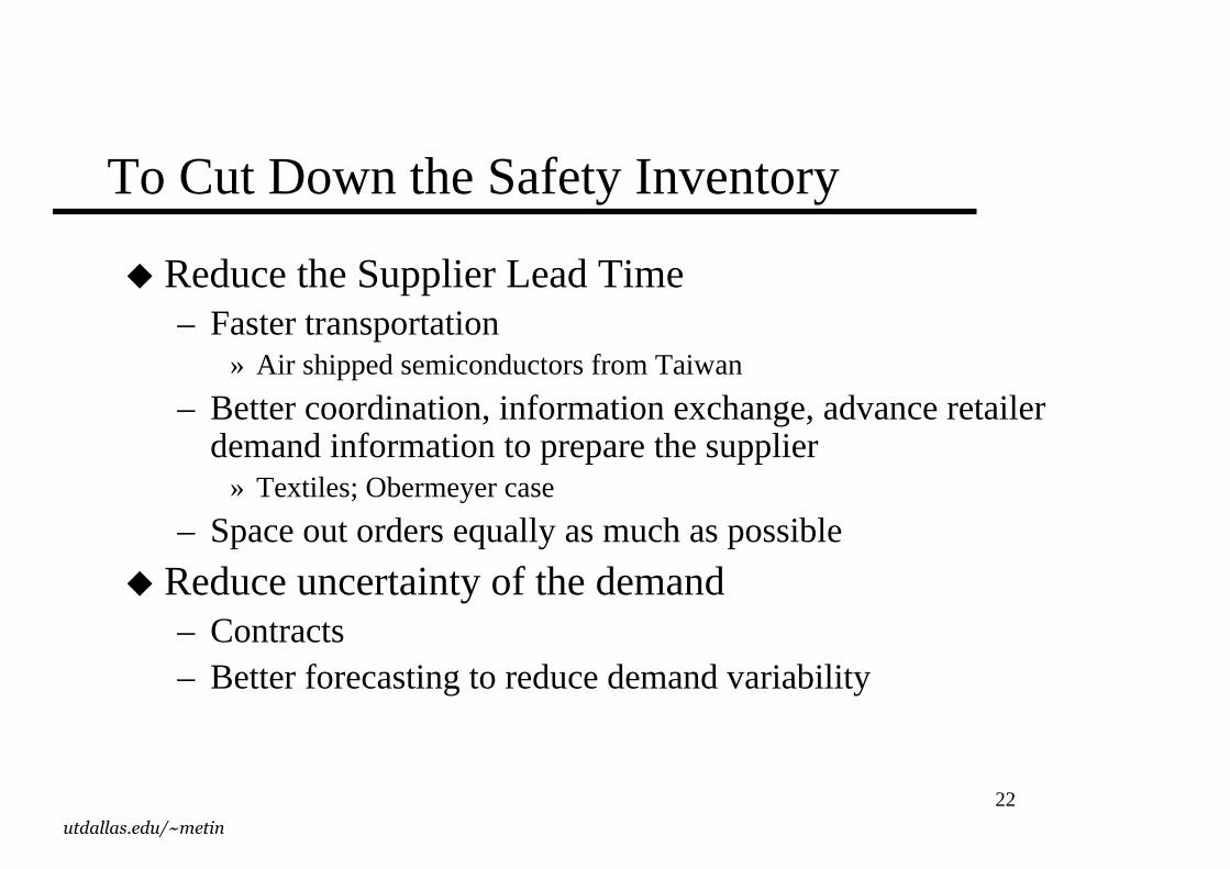
To Cut Down the Safety Inventory

� Reduce the Supplier Lead Time– Faster transportation

» Air shipped semiconductors from Taiwan

– Better coordination, information exchange, advance retailer demand information to prepare the supplier

» Textiles; Obermeyer case

– Space out orders equally as much as possible

� Reduce uncertainty of the demand– Contracts– Better forecasting to reduce demand variability


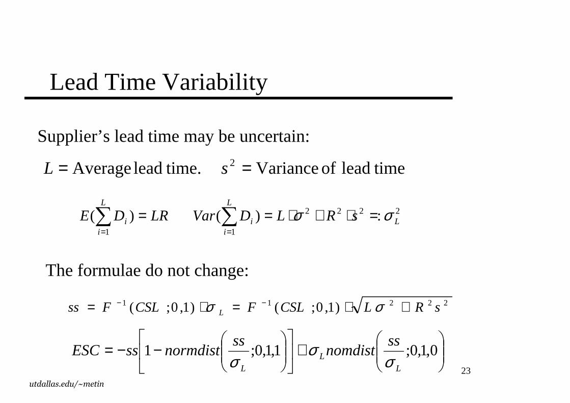
Lead Time Variability

2222

11

:)( )( L

L

ii

L

ii sRLDVarLRDE σσ =⋅+⋅== ∑∑

==

Supplier’s lead time may be uncertain:

timelead of Variance time.lead Average 2 == sL

22211 )1,0;()1,0;( sRLCSLFCSLFss L +⋅=⋅= −− σσ

+

−−= 0,1,0;1,1,0;1L

LL

ssnomdist

ssnormdistssESC

σσ

σ

The formulae do not change:


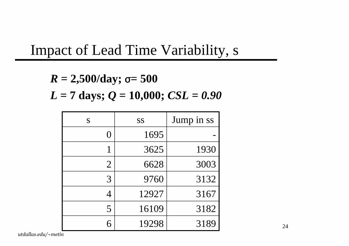
Impact of Lead Time Variability, s

R = 2,500/day; σσσσ= 500

L = 7 days; Q = 10,000; CSL = 0.90

3189192986

3182161095

3167129274

313297603

300366282

193036251

-16950

Jump in sssss


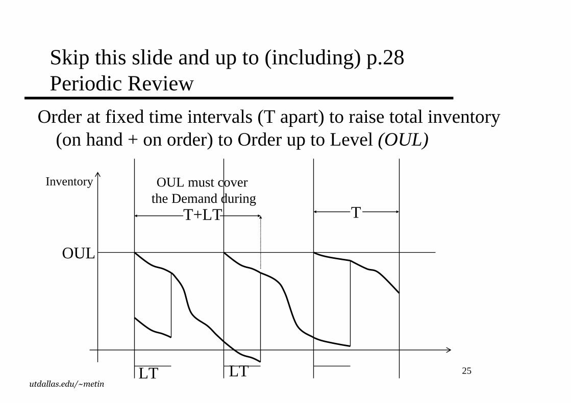
Skip this slide and up to (including) p.28Periodic Review

Order at fixed time intervals (T apart) to raise total inventory(on hand + on order) to Order up to Level (OUL)

Inventory

OUL

LT

T

LT

T+LT

OUL must cover the Demand during


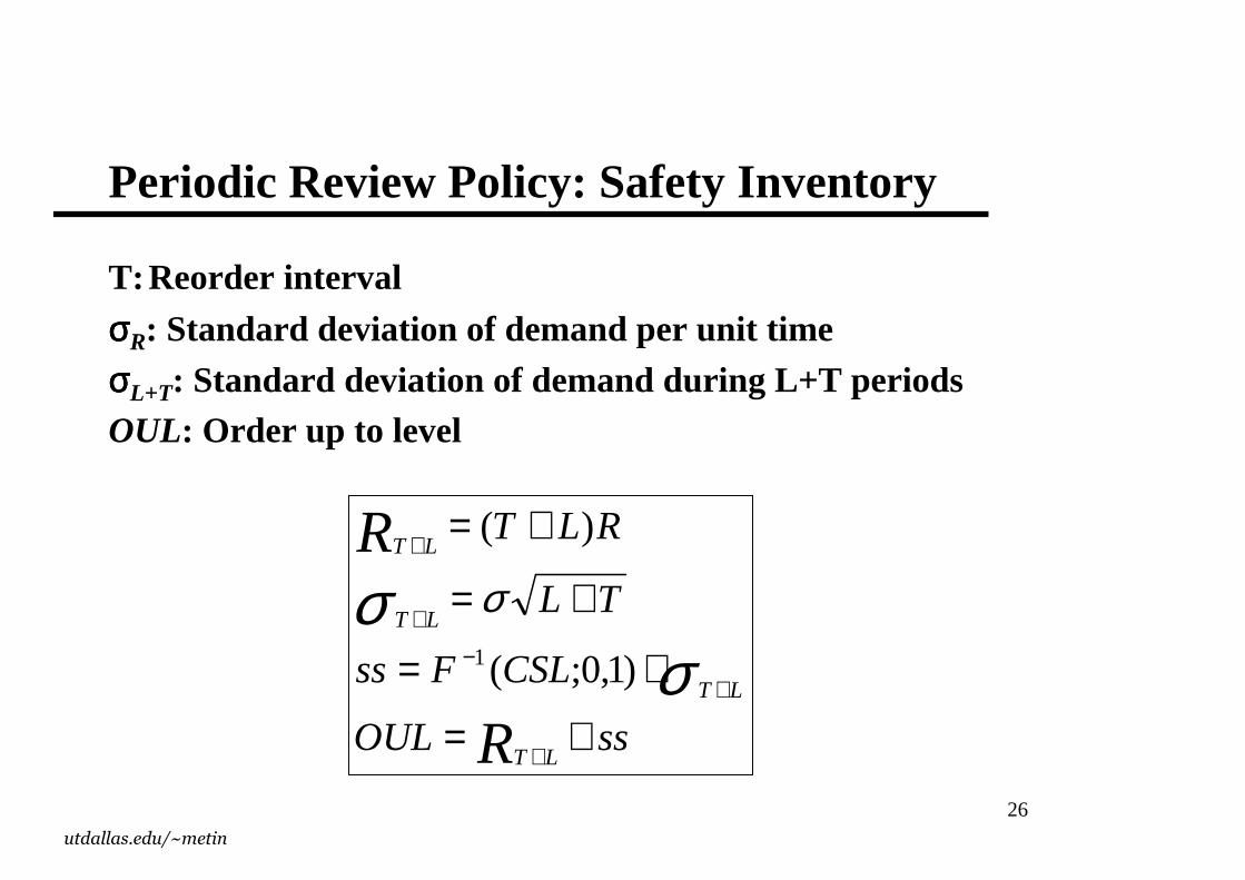
Per iodic Review Policy: Safety Inventory

T: Reorder interval

σσσσR: Standard deviation of demand per unit timeσσσσL+T: Standard deviation of demand dur ing L+T per iodsOUL: Order up to level

ssOUL

CSLFss

TL

RLT

R

R

LT

LT

LT

LT

+=

⋅=

+=

+=

+

+−

+

+

σσ σ

)1,0;(

)(

1


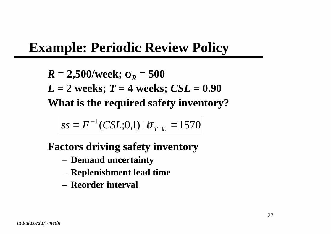
Example: Per iodic Review Policy

R = 2,500/week; σσσσR = 500L = 2 weeks; T = 4 weeks; CSL = 0.90What is the required safety inventory?

Factors dr iving safety inventory– Demand uncer tainty– Replenishment lead time– Reorder interval

1570)1,0;(1 =⋅= +−

LTCSLFss σ


Periodic vs Continuous Review

� Periodic review ss covers the uncertainty over [0,T+L], T periods more than ss in continuous case.

� Periodic review ss is larger.

� Continuous review is harder to implement, use it for high-sales-value per time products


Methods of Accurate Response to Var iability

� Physical Centralization

� Information centralization

– Virtual aggregation, Barnes&Nobles stores

� Specialization, what to aggregate

� Product substitution

� Raw material commonality - postponement


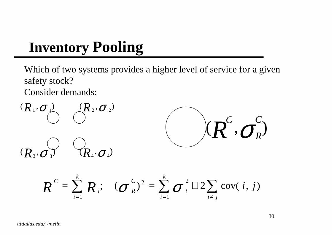
Inventory Pooling

∑∑∑≠==

+==ji

k

ii

C

R

k

ii

CjiRR ),cov(2)(;

1

22

1σσ

),(11 σR

),( σC

R

C

R

Which of two systems provides a higher level of service for a given safety stock? Consider demands:

),(33 σR

),(22 σR

),(44 σR


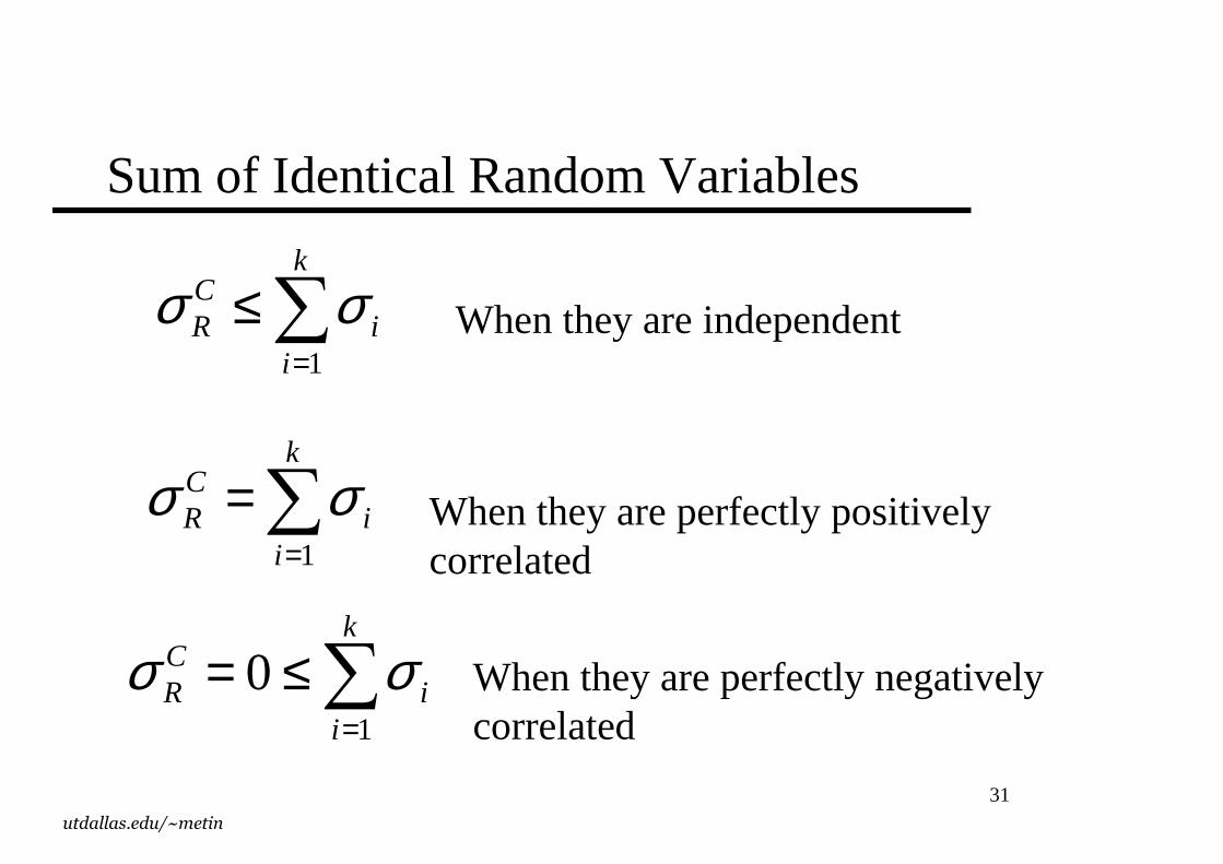
Sum of Identical Random Variables

∑=

≤k

ii

CR

1

σσ

∑=

=k

ii

CR

1

σσ

When they are independent

When they are perfectly positively correlated

∑=

≤=k

ii

CR

1

0 σσ When they are perfectly negatively correlated


Factors Affecting Value of Aggregation

� Demand Correlation, aggregation is helpful almost always except when products are positively correlated

� Coefficient of Variation of demand: Do not bother to aggregate if the variance is relatively small to begin with.


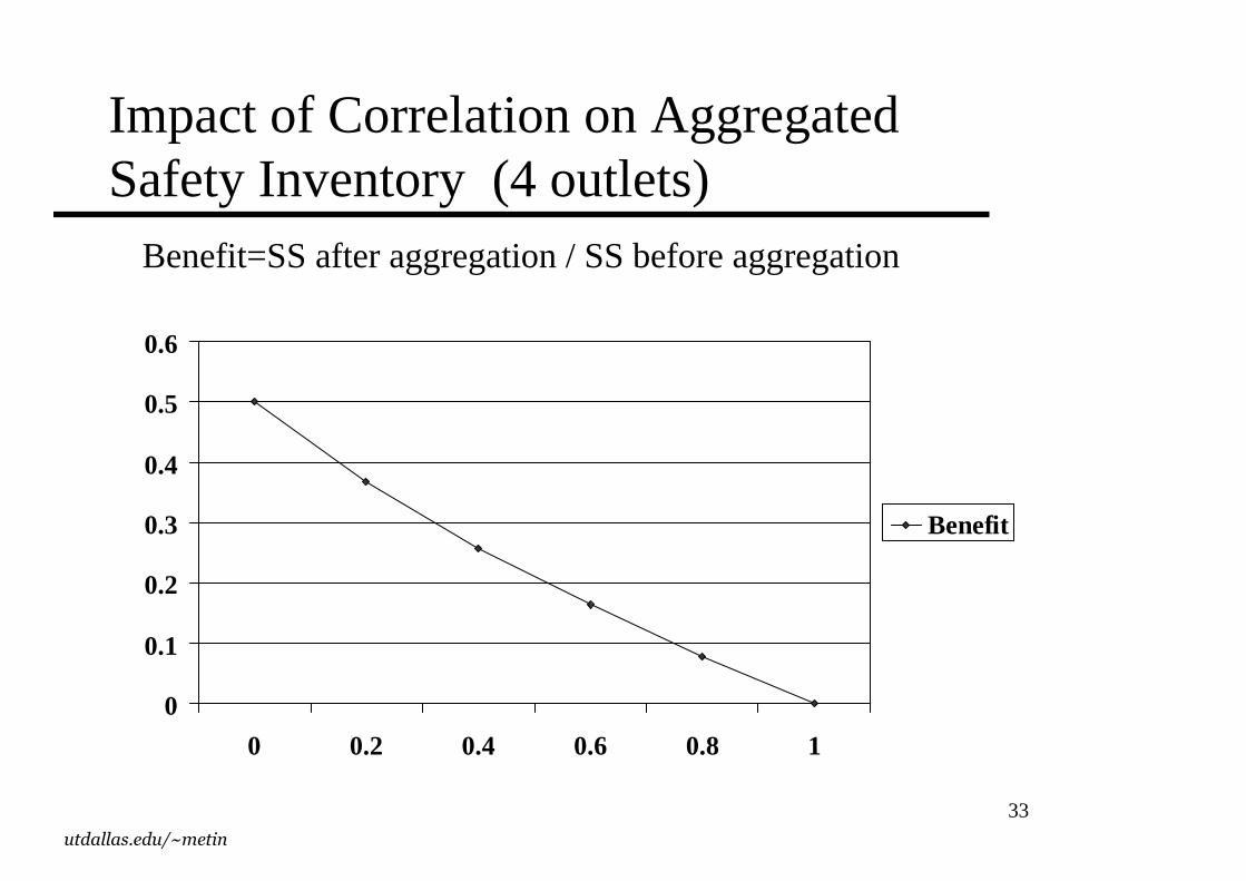
Impact of Correlation on Aggregated Safety Inventory (4 outlets)

0

0.1

0.2

0.3

0.4

0.5

0.6

0 0.2 0.4 0.6 0.8 1

Benefit

Benefit=SS after aggregation / SS before aggregation


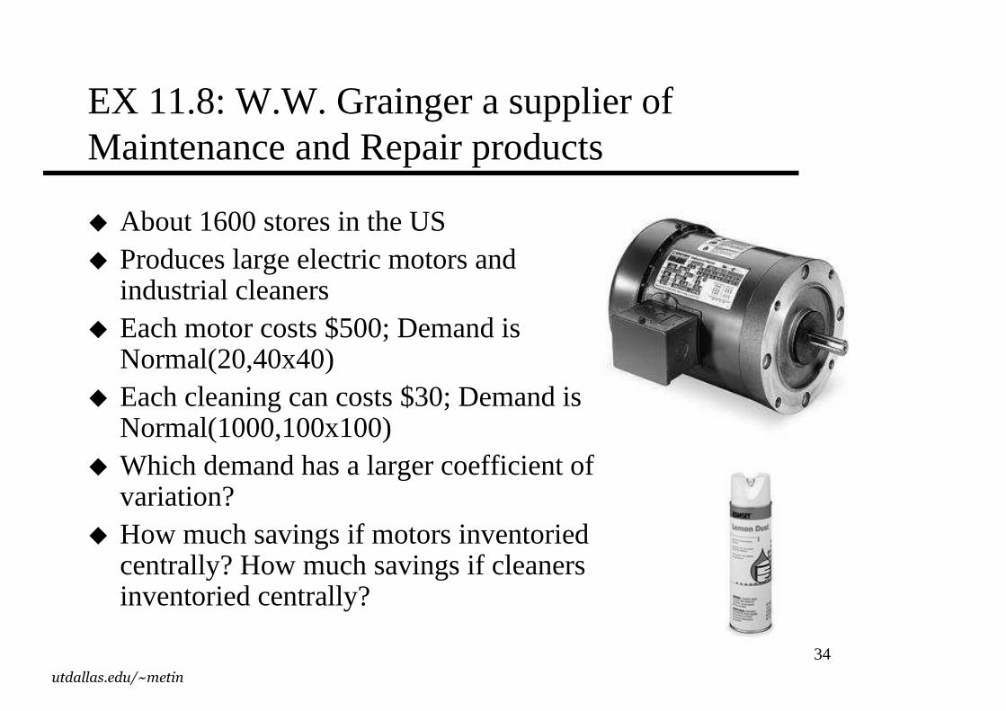
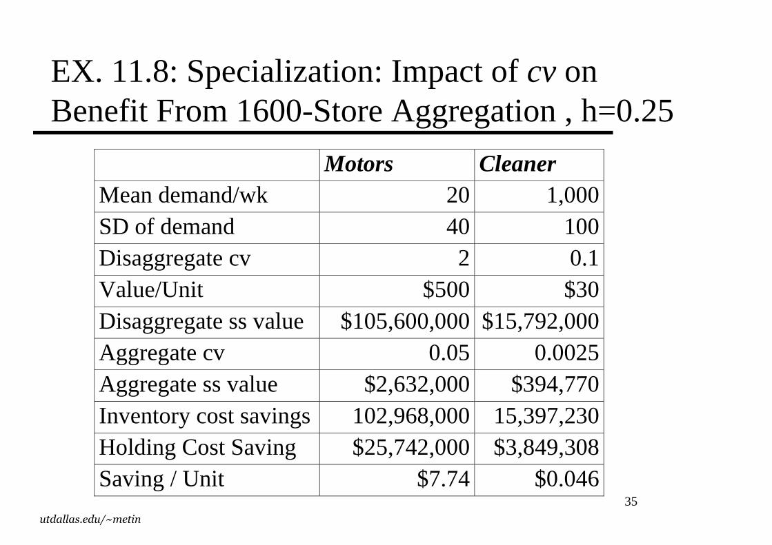
EX 11.8: W.W. Grainger a supplier of Maintenance and Repair products

� About 1600 stores in the US� Produces large electric motors and

industrial cleaners� Each motor costs $500; Demand is

Normal(20,40x40)� Each cleaning can costs $30; Demand is

Normal(1000,100x100)� Which demand has a larger coefficient of

variation?� How much savings if motors inventoried

centrally? How much savings if cleaners inventoried centrally?


EX. 11.8: Specialization: Impact of cv on Benefit From 1600-Store Aggregation , h=0.25

Motors Cleaner Mean demand/wk 20 1,000 SD of demand 40 100 Disaggregate cv 2 0.1 Value/Unit $500 $30 Disaggregate ss value $105,600,000 $15,792,000 Aggregate cv 0.05 0.0025 Aggregate ss value $2,632,000 $394,770 Inventory cost savings 102,968,000 15,397,230 Holding Cost Saving $25,742,000 $3,849,308 Saving / Unit $7.74 $0.046


Slow vsFast Moving Items

� Low demand = Slow moving items, vice versa.

� Slow moving items have high coefficient of variation, vice versa.

� Stock slow moving items at a central store

Buying a best seller at Amazon.com vs. a Supply Chain book vs. aBanach spaces book, which has a shorter delivery time?

- “Case Interview” books are not in our sku list. You must check with our central stores.

- Store keeper at Barnes and Nobles at Collin Creek, March 2002.


Product Substitution

� Manufacturer driven� Customer driven

Consider: The price of the products substituted for each other and the demand correlations

� One-way substitution – Army boots. Aggregate?

� Two-way substitution: – Grainger motors; water pumps model DN vs IT. – Similar products, can customer detect specifications.

If products are very similar, why not to eliminate?


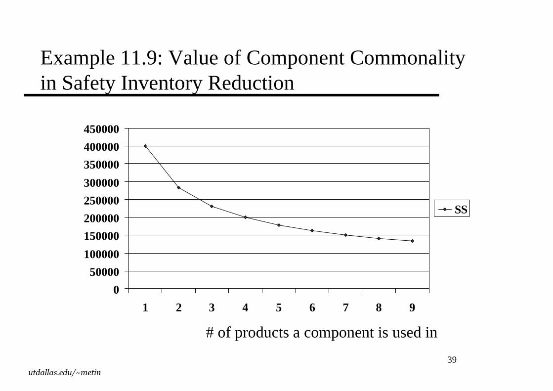
Component commonality. Ex. 11.9

� Dell producing 27 products with 3 components (processor, memory, hard drive)

� No product commonality: A component is used in only 1 product. 27 component versions are required for each component. A total of 3*27 = 81 distinct components is required.

� Max component commonality. Only three distinct versions for each component. Each combination of components is a distinct product. A component is used in 9 products.

� Component commonality provides inventory aggregation.


Example 11.9: Value of Component Commonalityin Safety Inventory Reduction

0

50000

100000

150000

200000

250000

300000

350000

400000

450000

1 2 3 4 5 6 7 8 9

SS

# of products a component is used in


Advantages of Standardization

� Fewer parts to deal with in inventory & manufacturing

– Less costly to fill orders from inventory

� Reduced training costs and time

� More routine purchasing, handling, and inspection procedures

� Opportunities for long production runs, automation

� Need for fewer parts justifies increased expenditures on perfecting designs and improving quality control procedures.


Disadvantages of Standardization

� Decreased variety results in less consumer appeal.

� Designs may be frozen with too many imperfections remaining.

– US wireless communication standards vs Europe’s

� High cost of design changes increases resistance to improvements

– Keyboards: We are using a suboptimal qwerty keyboard. Even moreinterestingly countries using languages other than English also mostly use qwerty keyboard.


Mass customization:– A strategy of producing standardized goods or services,

but incorporating some degree of customization– Modular design– Delayed differentiation

Mass Customization


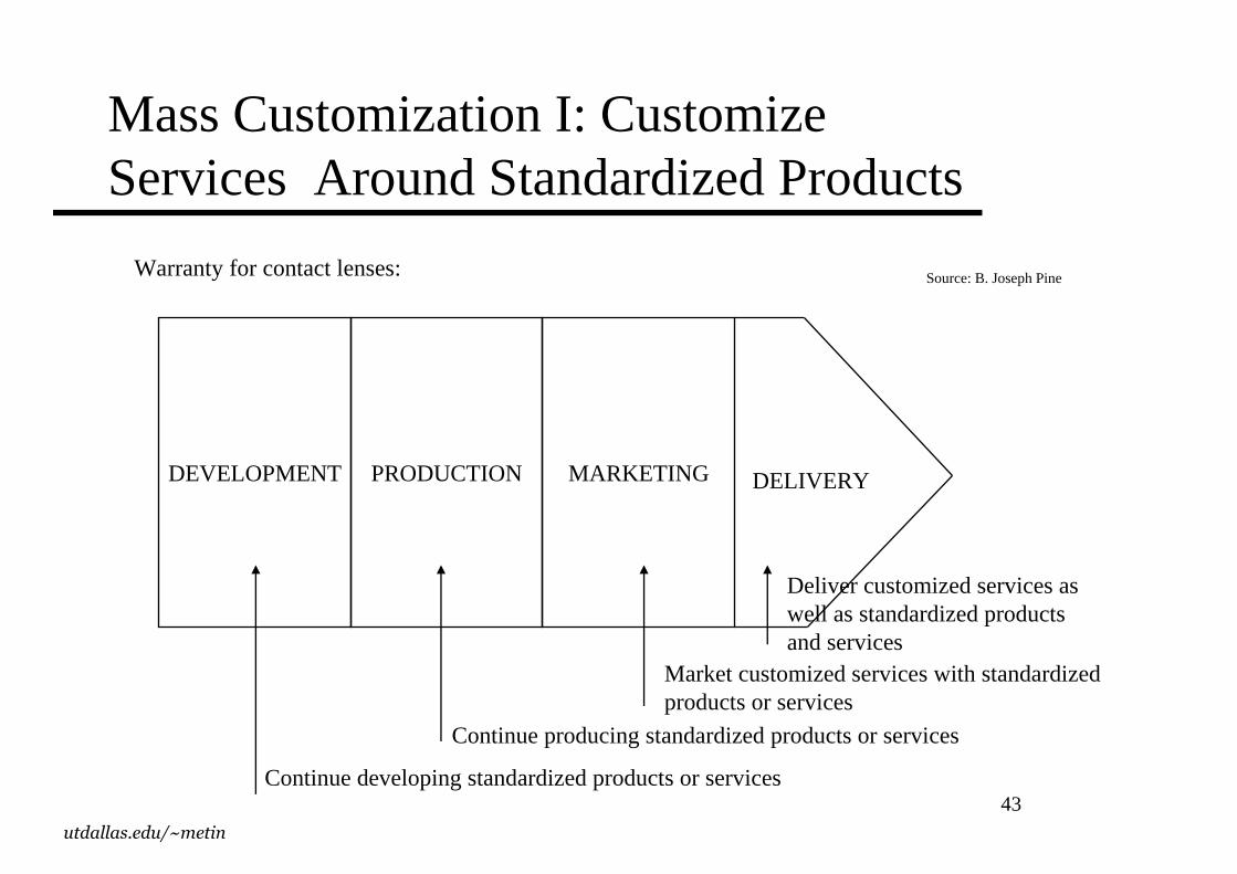
Mass Customization I: Customize Services Around Standardized Products

DEVELOPMENT PRODUCTION MARKETING DELIVERY

Deliver customized services aswell as standardized productsand services

Market customized services with standardizedproducts or services

Continue producing standardized products or services

Continue developing standardized products or services

Source: B. Joseph PineWarranty for contact lenses:


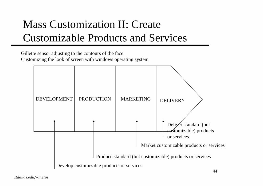
Mass Customization II: Create Customizable Products and Services


Deliver standard (but customizable) productsor services

Market customizable products or services

Produce standard (but customizable) products or services

Develop customizable products or services

Gillette sensor adjusting to the contours of the faceCustomizing the look of screen with windows operating system


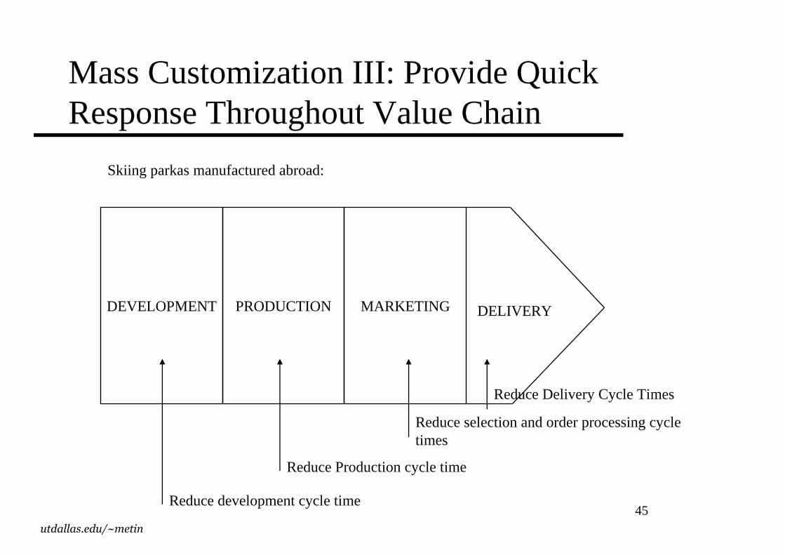
Mass Customization III: Provide Quick ResponseThroughout Value Chain


Reduce Delivery Cycle Times

Reduce selection and order processing cycle times

Reduce Production cycle time

Reduce development cycle time

Skiing parkas manufactured abroad:


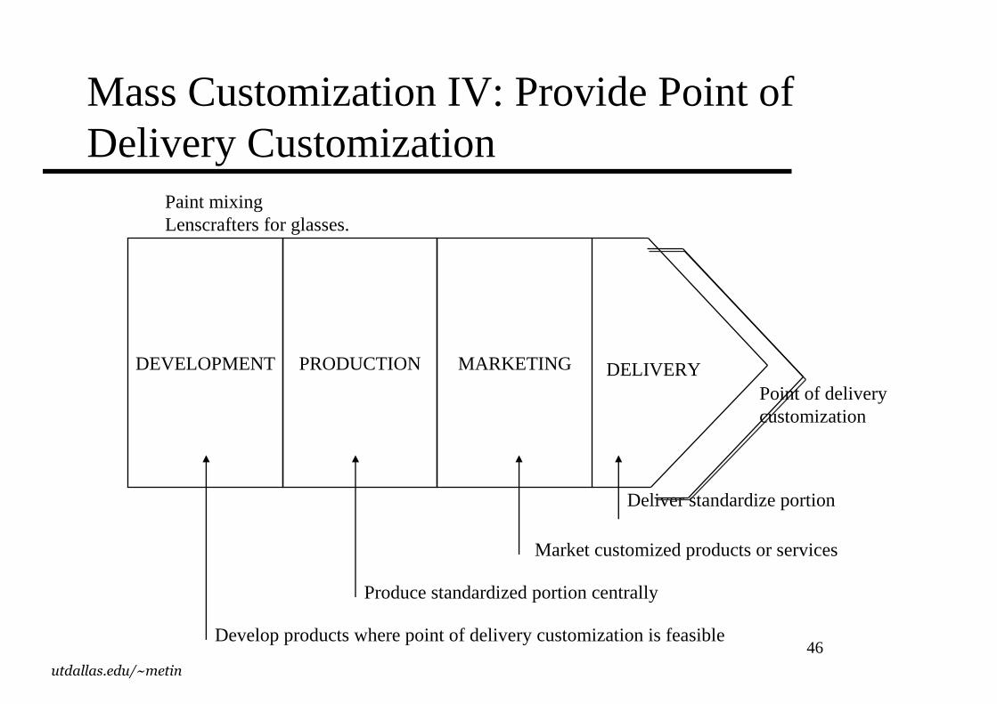
Mass Customization IV: Provide Point of Delivery Customization


Deliver standardize portion

Market customized products or services

Produce standardized portion centrally

Develop products where point of delivery customization is feasible

Point of deliverycustomization

Paint mixingLenscrafters for glasses.


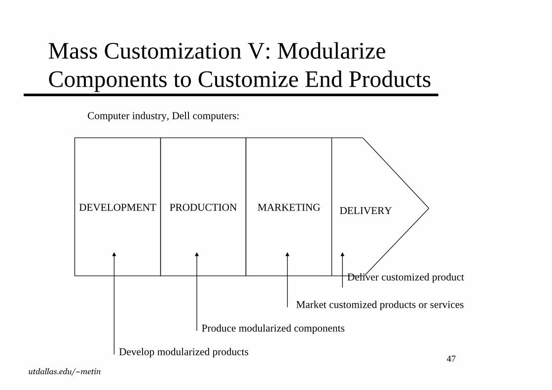
Mass Customization V: Modularize Components to Customize End Products


Deliver customized product

Market customized products or services

Produce modularized components

Develop modularized products

Computer industry, Dell computers:


Modular Design

Modular design is a form of standardization in which component parts are subdivided into modules that are easily replaced or interchanged.

– A bad example: Earlier Ford SUVs shared the lower body with Fordcars

It allows:

– easier diagnosis and remedy of failures

– easier repair and replacement

– simplification of manufacturing and assembly


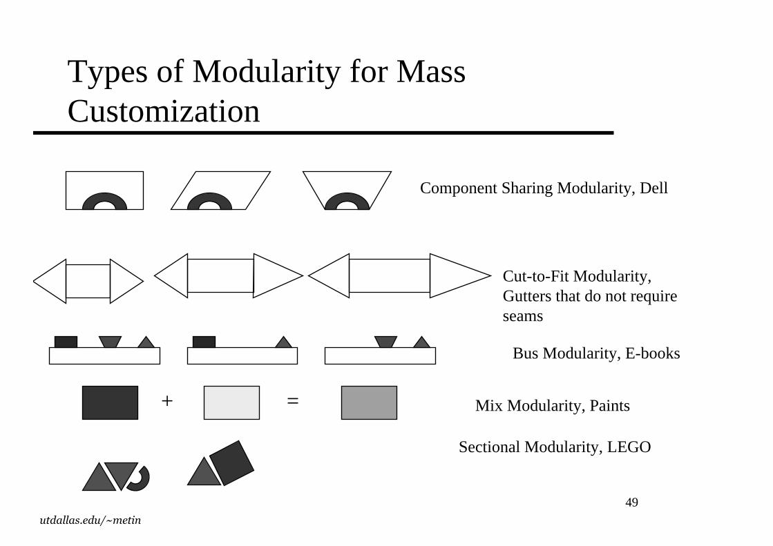
Types of Modularity for Mass Customization

Component Sharing Modularity, Dell

Cut-to-Fit Modularity, Gutters that do not require seams

Bus Modularity, E-books

Mix Modularity, Paints

Sectional Modularity, LEGO

+ =


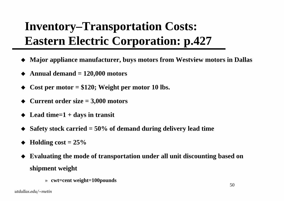
Inventory–Transpor tation Costs: Eastern Electr ic Corporation: p.427� Major appliance manufacturer , buys motors from Westview motors in Dallas

� Annual demand = 120,000 motors

� Cost per motor = $120; Weight per motor 10 lbs.

� Current order size = 3,000 motors

� Lead time=1 + days in transit

� Safety stock carr ied = 50% of demand dur ing delivery lead time

� Holding cost = 25%

� Evaluating the mode of transpor tation under all unit discounting based on

shipment weight

» cwt=cent weight=100pounds


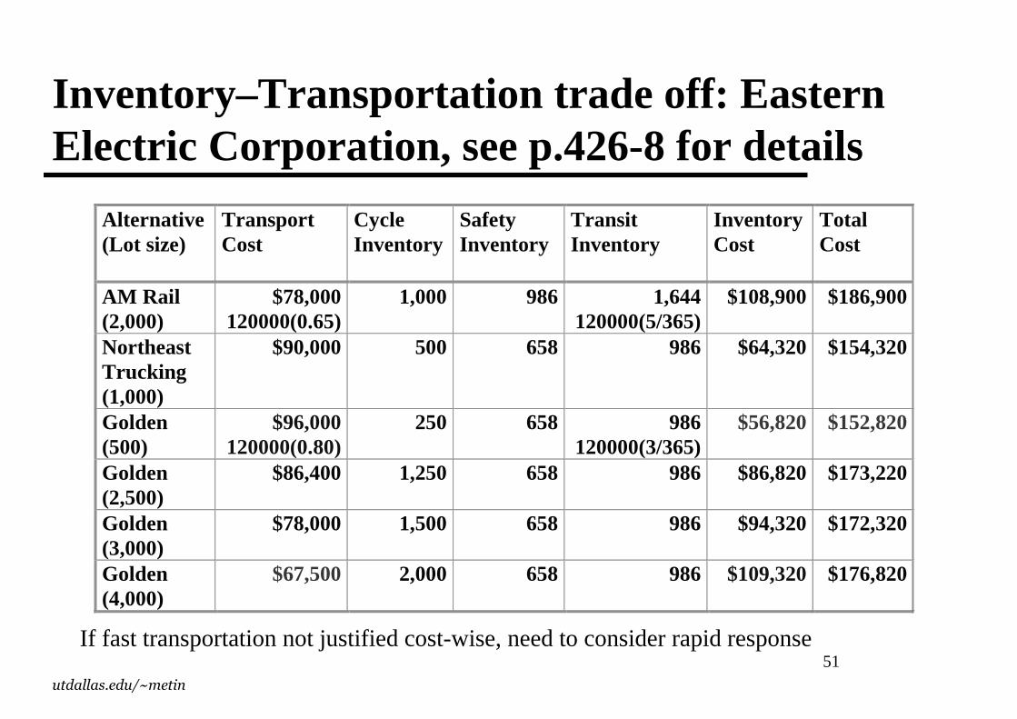
Inventory–Transpor tation trade off: Eastern Electr ic Corporation, see p.426-8 for details

Alternative (Lot size)

Transpor t Cost

Cycle Inventory

Safety Inventory

Transit Inventory

Inventory Cost

Total Cost

AM Rail (2,000)

$78,000 120000(0.65)

1,000 986 1,644 120000(5/365)

$108,900 $186,900

Nor theast Trucking (1,000)

$90,000 500 658 986 $64,320 $154,320

Golden (500)

$96,000 120000(0.80)

250 658 986 120000(3/365)

$56,820 $152,820

Golden (2,500)

$86,400 1,250 658 986 $86,820 $173,220

Golden (3,000)

$78,000 1,500 658 986 $94,320 $172,320

Golden (4,000)

$67,500 2,000 658 986 $109,320 $176,820

If fast transportation not justified cost-wise, need to consider rapid response


Physical Inventory Aggregation: Inventory vs. Transportation cost: p.428

� HighMed Inc. producer of medical equipment sold directly to doctors

� Located in Wisconsin serves 24 regions in USA

� As a result of physical aggregation– Inventory costs decrease

– Inbound transportation cost decreases» Inbound lots are larger

– Outbound transportation cost increases


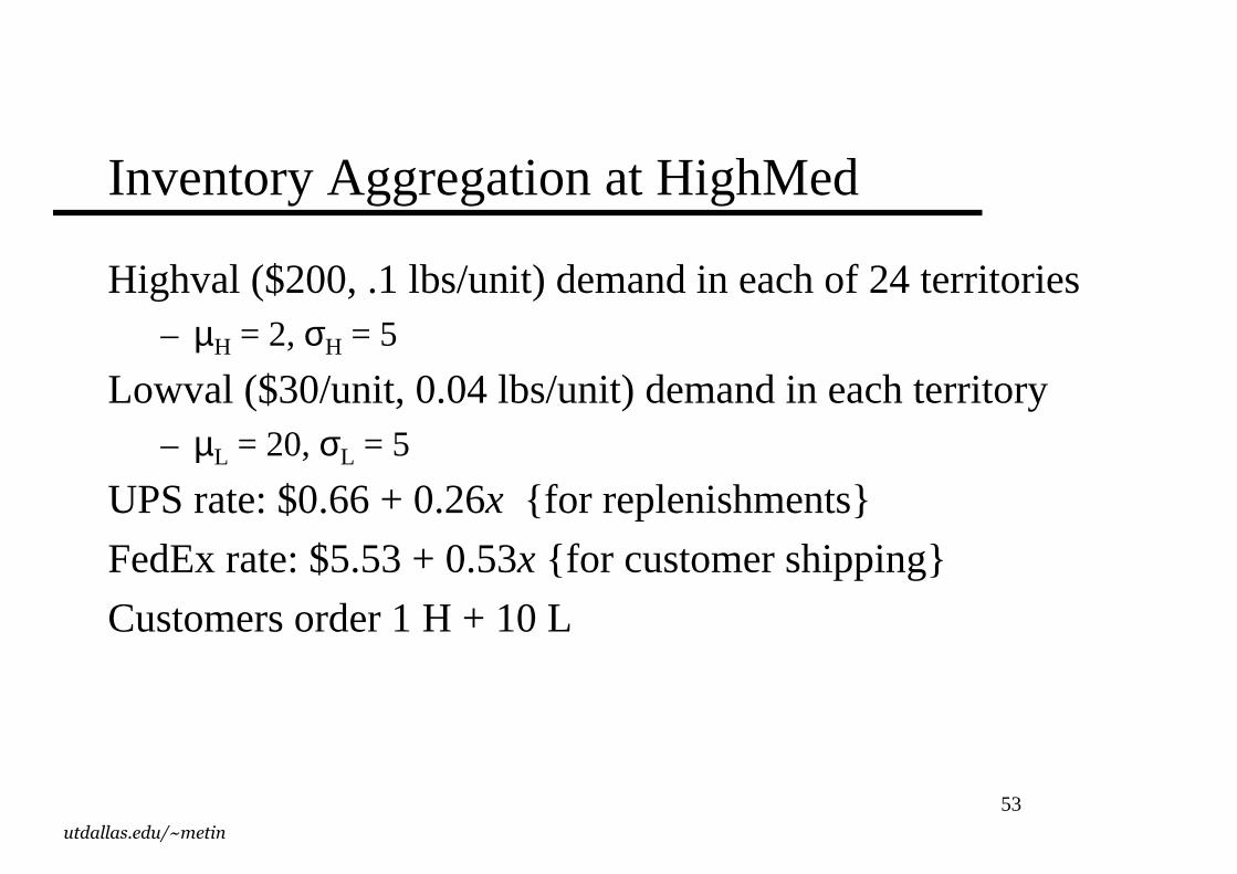
Inventory Aggregation at HighMed

Highval ($200, .1 lbs/unit) demand in each of 24 territories– µH = 2, σH = 5

Lowval ($30/unit, 0.04 lbs/unit) demand in each territory– µL = 20, σL = 5

UPS rate: $0.66 + 0.26x { for replenishments}

FedEx rate: $5.53 + 0.53x { for customer shipping}

Customers order 1 H + 10 L


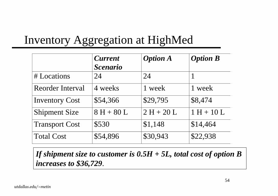
Inventory Aggregation at HighMed

Current Scenario

Option A Option B

# Locations 24 24 1

Reorder Interval 4 weeks 1 week 1 week

Inventory Cost $54,366 $29,795 $8,474

Shipment Size 8 H + 80 L 2 H + 20 L 1 H + 10 L

Transport Cost $530 $1,148 $14,464

Total Cost $54,896 $30,943 $22,938

If shipment size to customer is 0.5H + 5L, total cost of option B increases to $36,729.


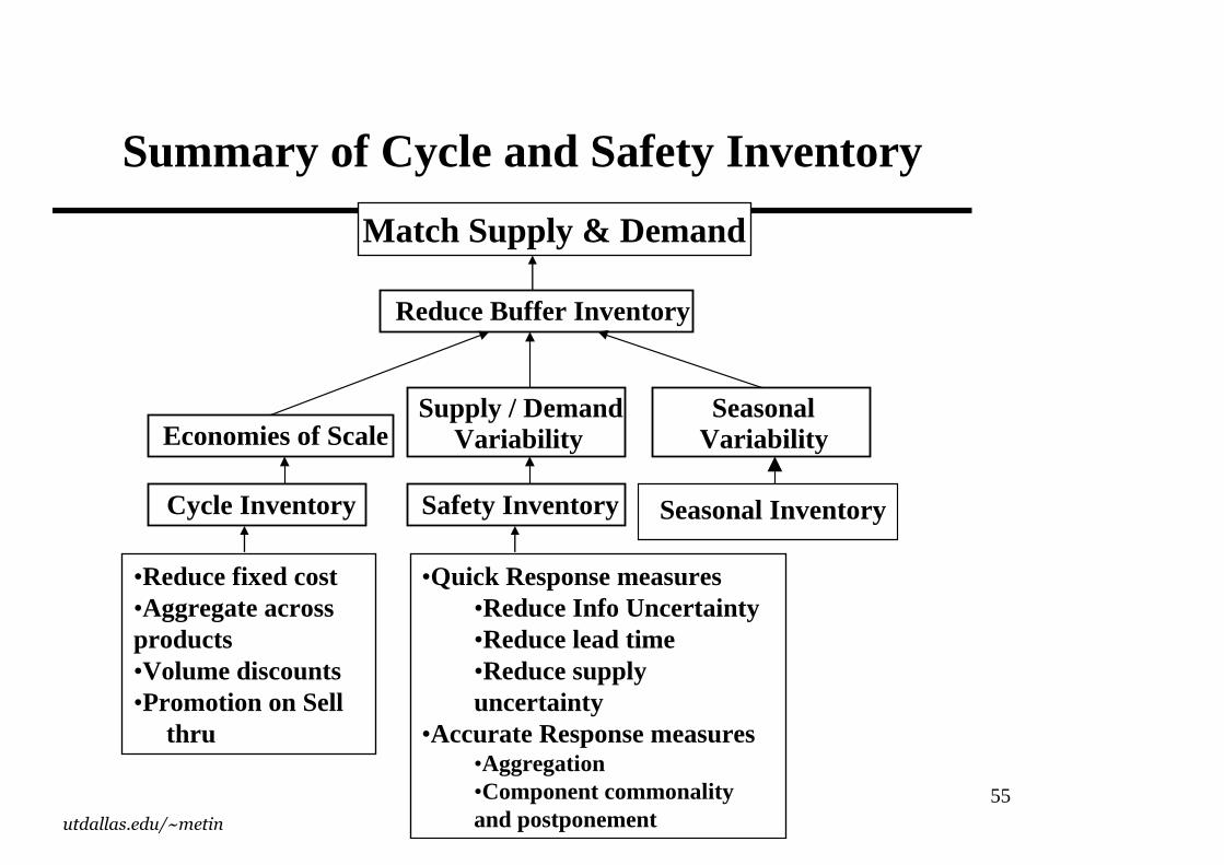
Summary of Cycle and Safety Inventory

Reduce Buffer Inventory

Economies of ScaleSupply / Demand

Var iabilitySeasonal

Var iability

Cycle Inventory Safety Inventory Seasonal Inventory

Match Supply & Demand

•Reduce fixed cost•Aggregate across products•Volume discounts•Promotion on Sell

thru

•Quick Response measures•Reduce Info Uncer tainty•Reduce lead time•Reduce supply uncer tainty

•Accurate Response measures•Aggregation•Component commonality and postponement

Documents

Safety Inventories - The University of Texas at Dallasmetin/FuJen/Folios/scstocinventory_s.pdf · Safety Inventories Chapter 11 of Chopra. ... If Safety inventory is up, ... Buying