1

Mon. Apr. 02, 2018

• Satellite Gravity Measurements (GRACE, GRAIL)– Use slides posted for Friday

• Linear (Spectral) Mixing

• Reading: Chapter 9 (“Environmental” Remote Sensing”)– Once again -- Satellites old but principles still apply

2

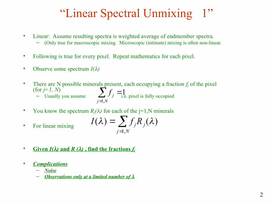
“Linear Spectral Unmixing 1”

• Linear: Assume resulting spectra is weighted average of endmember spectra. – (Only true for macroscopic mixing. Microscopic (intimate) mixing is often non-linear.

• Following is true for every pixel. Repeat mathematics for each pixel.

• Observe some spectrum I()

• There are N possible minerals present, each occupying a fraction fj of the pixel (for j=1, N)

– Usually you assume i.e. pixel is fully occupied

• You know the spectrum Rj() for each of the j=1,N minerals

• For linear mixing

• Given I() and R () , find the fractions fj

• Complications– Noise– Observations only at a limited number of

Nj

jf,1

1

Nj

jjRfI,1

)()(

3

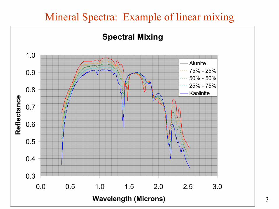
Mineral Spectra: Example of linear mixing

Spectral Mixing

0.3

0.4

0.5

0.6

0.7

0.8

0.9

1.0

0.0 0.5 1.0 1.5 2.0 2.5 3.0

Wavelength (Microns)

Re

fle

cta

nc

e

Alunite75% - 25%50% - 50%25% - 75%Kaolinite

4

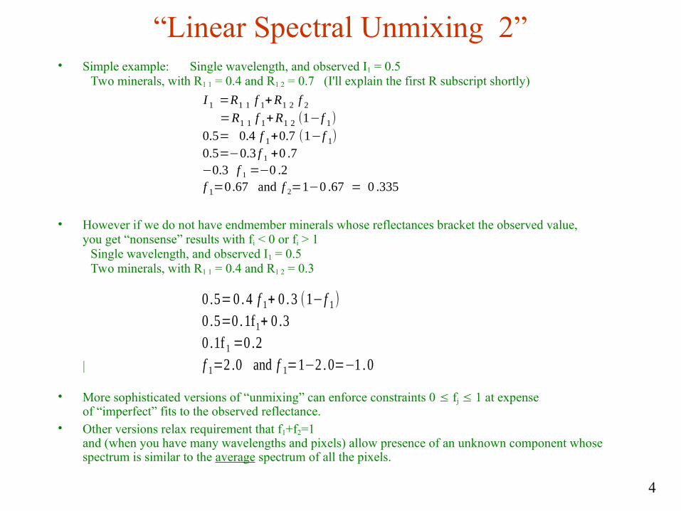
“Linear Spectral Unmixing 2”• Simple example: Single wavelength, and observed I1 = 0.5

Two minerals, with R1 1 = 0.4 and R1 2 = 0.7 (I'll explain the first R subscript shortly)

• However if we do not have endmember minerals whose reflectances bracket the observed value,you get “nonsense” results with fi < 0 or fi > 1

Single wavelength, and observed I1 = 0.5Two minerals, with R1 1 = 0.4 and R1 2 = 0.3

|

• More sophisticated versions of “unmixing” can enforce constraints 0 fj 1 at expenseof “imperfect” fits to the observed reflectance.

• Other versions relax requirement that f1+f2=1and (when you have many wavelengths and pixels) allow presence of an unknown component whose spectrum is similar to the average spectrum of all the pixels.

I 1 =R1 1 f 1+R1 2 f 2

=R1 1 f 1+R1 2 (1−f 1)

0.5= 0.4 f 1+0.7 (1−f 1)

0.5=−0.3 f 1 +0 .7−0.3 f 1 =−0 .2f 1=0.67 and f 2=1−0 .67 = 0 .335

0 .5=0 . 4 f 1+ 0 . 3 (1− f 1 )

0 .5=0 . 1f1+ 0 .30 .1f 1 =0 .2f 1=2 .0 and f 1=1−2 . 0=−1 .0

5

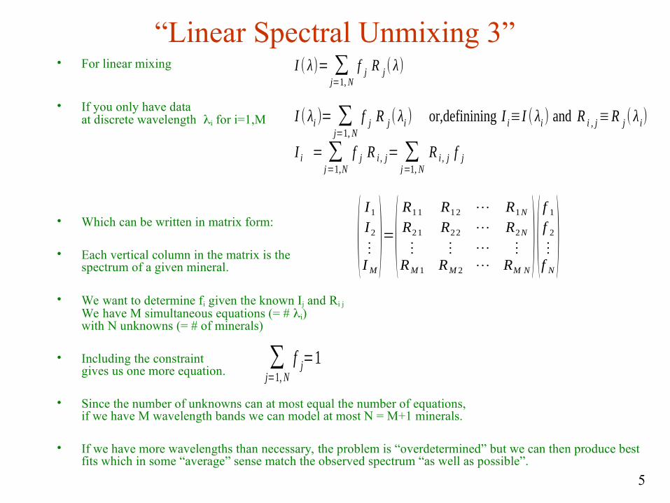
“Linear Spectral Unmixing 3”• For linear mixing

• If you only have data at discrete wavelength i for i=1,M

• Which can be written in matrix form:

• Each vertical column in the matrix is thespectrum of a given mineral.

• We want to determine fi given the known Ij and Ri j

We have M simultaneous equations (= # i)with N unknowns (= # of minerals)

• Including the constraintgives us one more equation.

• Since the number of unknowns can at most equal the number of equations,if we have M wavelength bands we can model at most N = M+1 minerals.

• If we have more wavelengths than necessary, the problem is “overdetermined” but we can then produce best fits which in some “average” sense match the observed spectrum “as well as possible”.

∑j=1,N

f j=1

I ( λ)= ∑j=1,N

f j R j ( λ)

I ( λi )= ∑j=1,N

f j R j ( λi ) or,definining I i≡I ( λi ) and R i , j≡R j ( λ i)

I i = ∑j=1,N

f j R i , j= ∑j=1,N

R i , j f j

(I1

I2

⋮

IM)=(

R11 R12 ⋯ R1N

R21 R22 ⋯ R2N

⋮ ⋮ ⋯ ⋮

RM 1 RM 2 ⋯ RM N

)(f 1

f 2

⋮

f N)

6

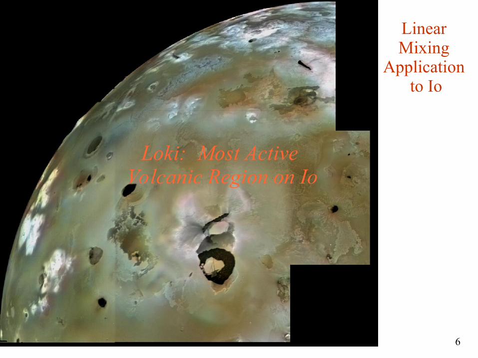
Linear Mixing

Application to Io

Loki: Most Active Volcanic Region on Io

7

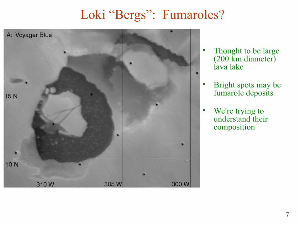
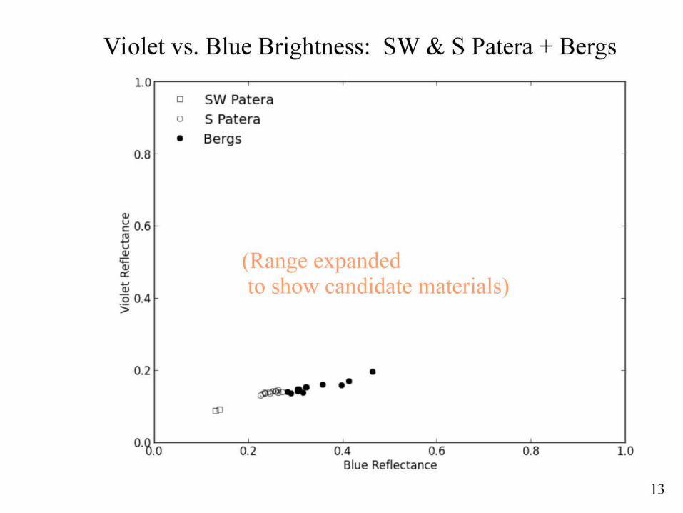
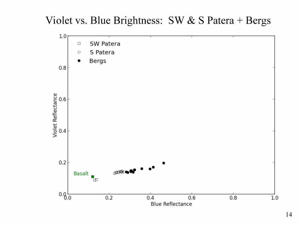
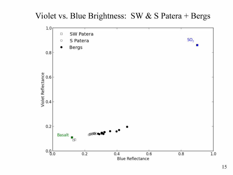
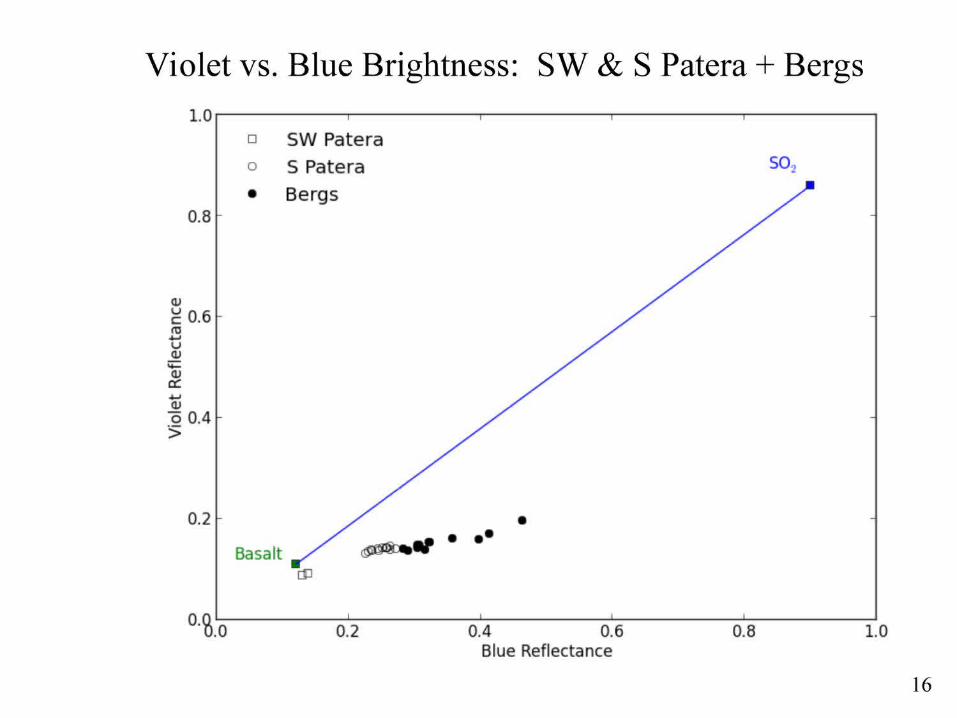
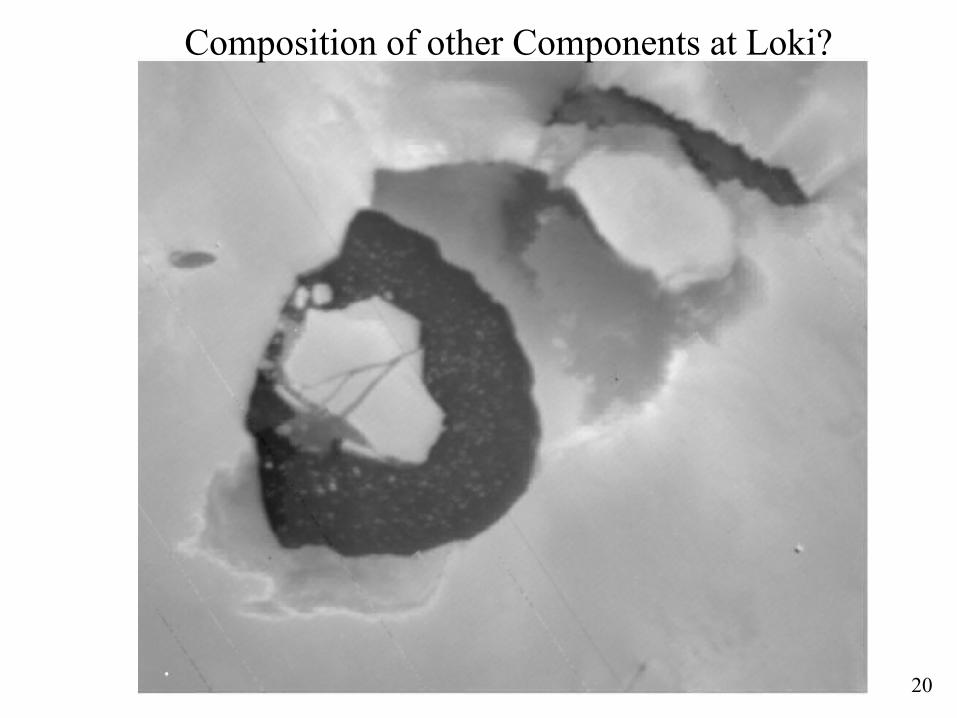
Loki “Bergs”: Fumaroles?

• Thought to be large (200 km diameter) lava lake

• Bright spots may be fumarole deposits

• We're trying to understand their composition

8

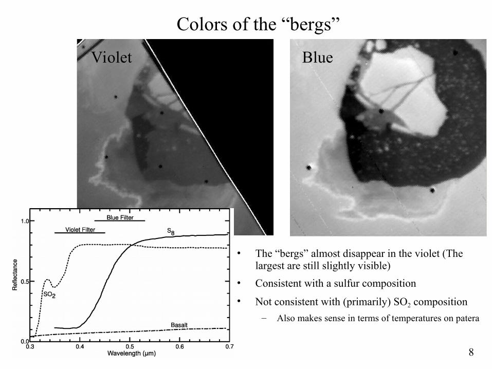
Colors of the “bergs”

BlueViolet

• The “bergs” almost disappear in the violet (The largest are still slightly visible)

• Consistent with a sulfur composition

• Not consistent with (primarily) SO2 composition

– Also makes sense in terms of temperatures on pateraSpectra from Moses & Nash

20

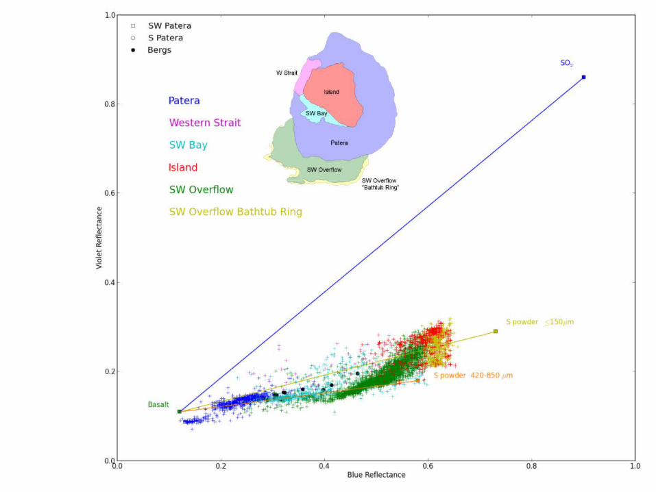
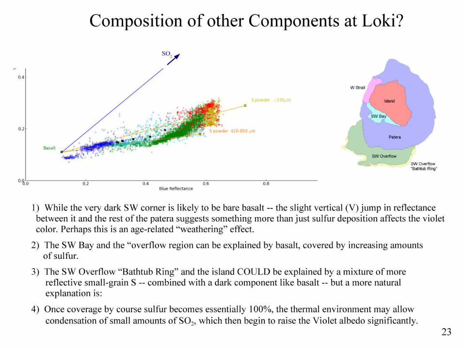
Composition of other Components at Loki?

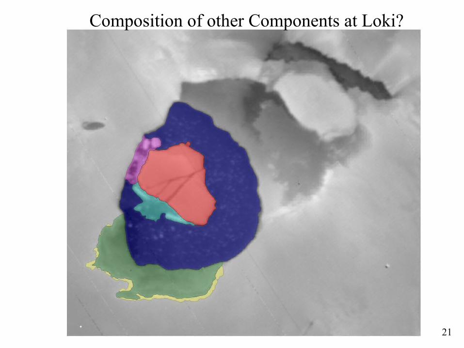
21

Composition of other Components at Loki?

24

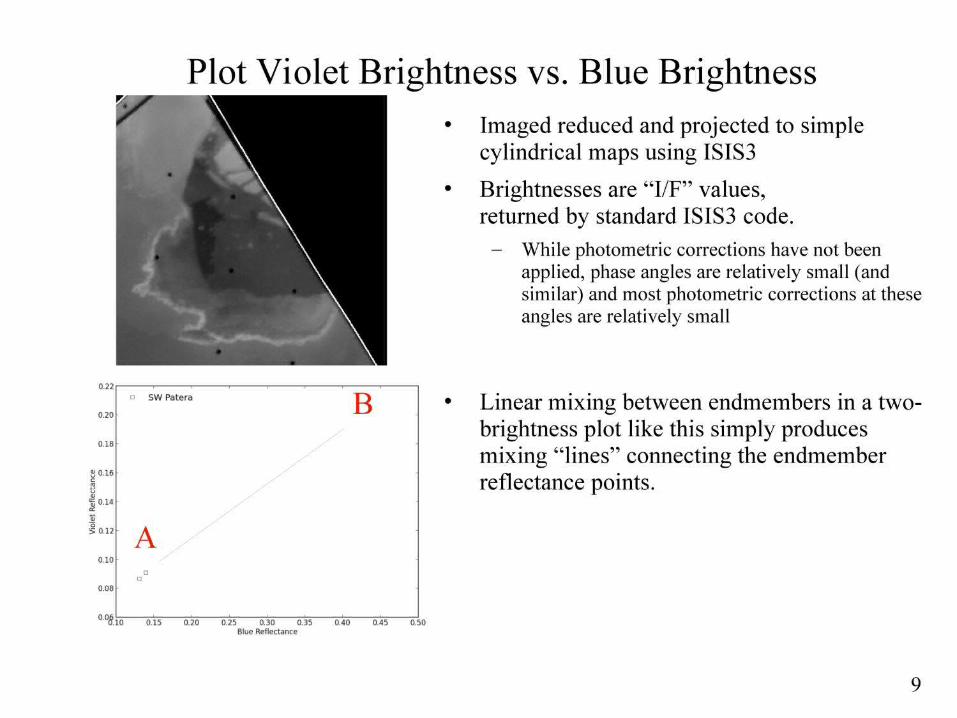
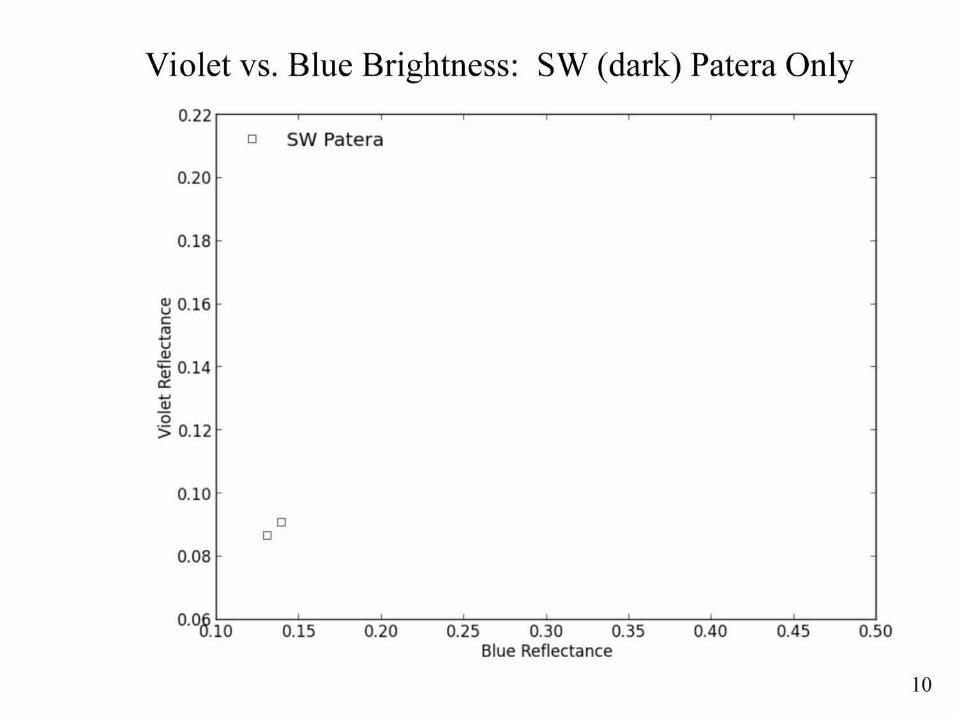
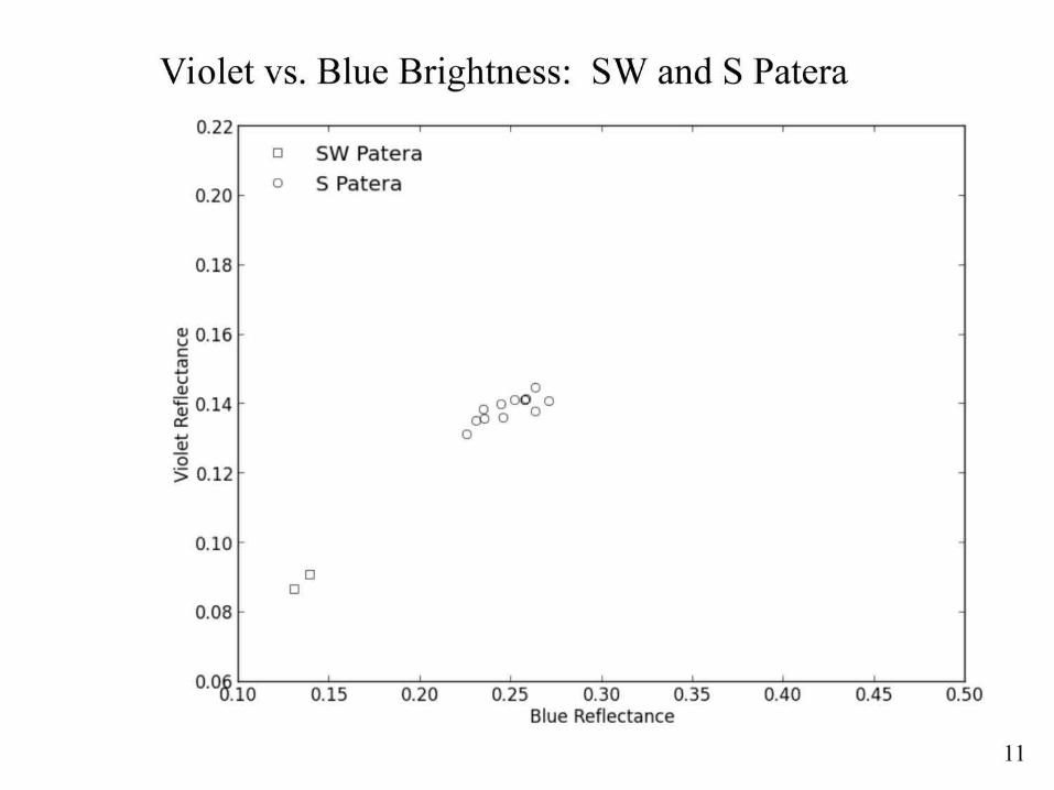
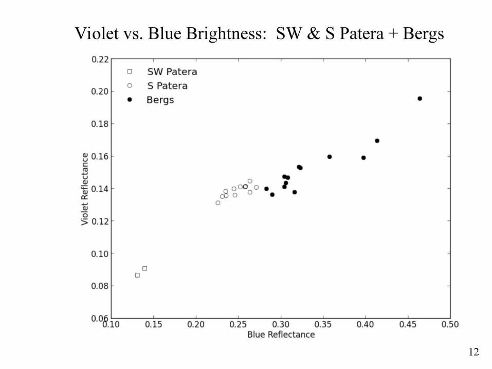
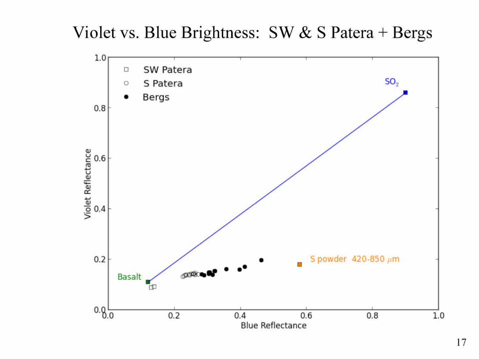
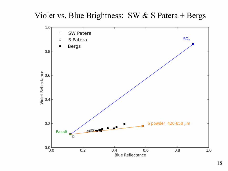
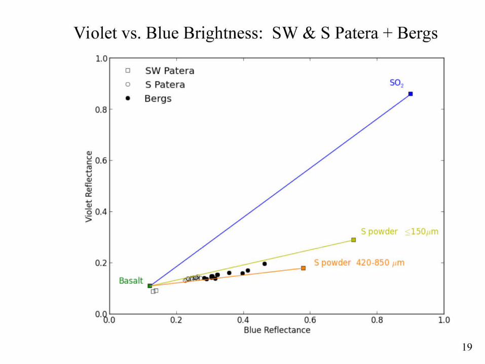
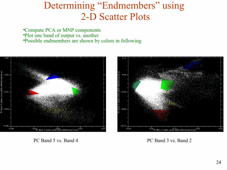
Determining “Endmembers” using 2-D Scatter Plots

•Compute PCA or MNP components•Plot one band of output vs. another•Possible endmembers are shown by colors in following

PC Band 5 vs. Band 4 PC Band 3 vs. Band 2