Embed Size (px)
Citation preview
1
Local improvement of GRACE gravity field solutions using SO(3)
representations M. Antoni & W. Keller
Institute of Geodesy, Universität Stuttgart, Germany
7. January 2012
2
1. GRACE mission
•Two satellites in the same orbit, separated along-track by about 200km.
•Continuously, measuring their relative velocity, with very high accuracy.
•Changes in the relative velocity are related to changes in gravity:
Courtesy of CSR
V (r, ✓,� ) =GM
R
1 +
1X
n=2
✓R
r
◆n+1 nX
m=�n
cnmYn,m(✓,� )
!
3
1. GRACE mission (cont.)
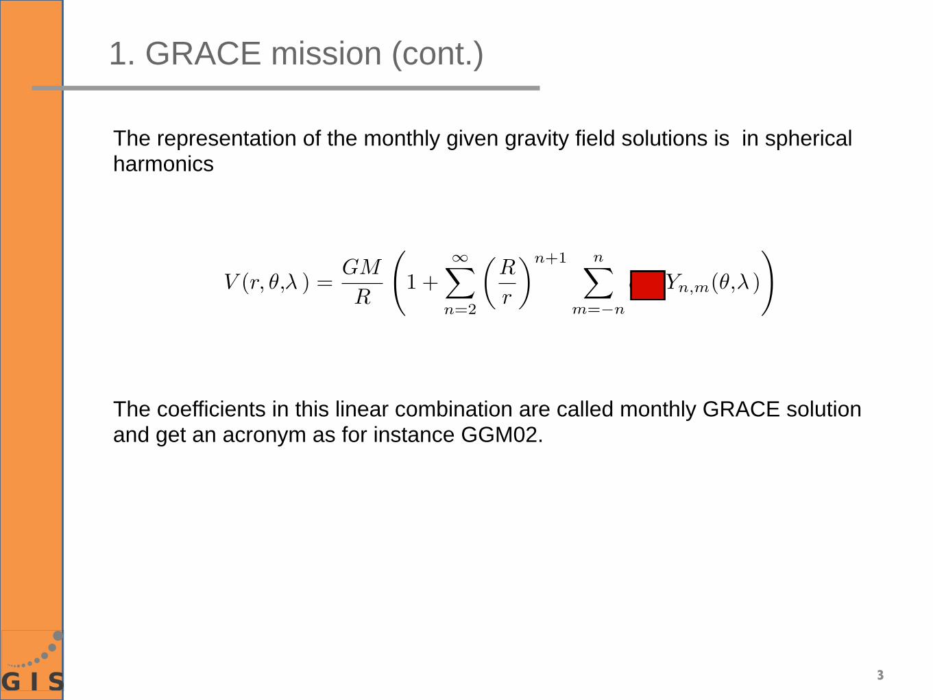
The representation of the monthly given gravity field solutions is in sphericalharmonics
The coefficients in this linear combination are called monthly GRACE solution and get an acronym as for instance GGM02.
52869,63 52869,632 52869,634 52869,636time [JD]
-5e-05
0
5e-05
0,0001
rang
e-ra
te d
iffer
ence
s [m
/s]
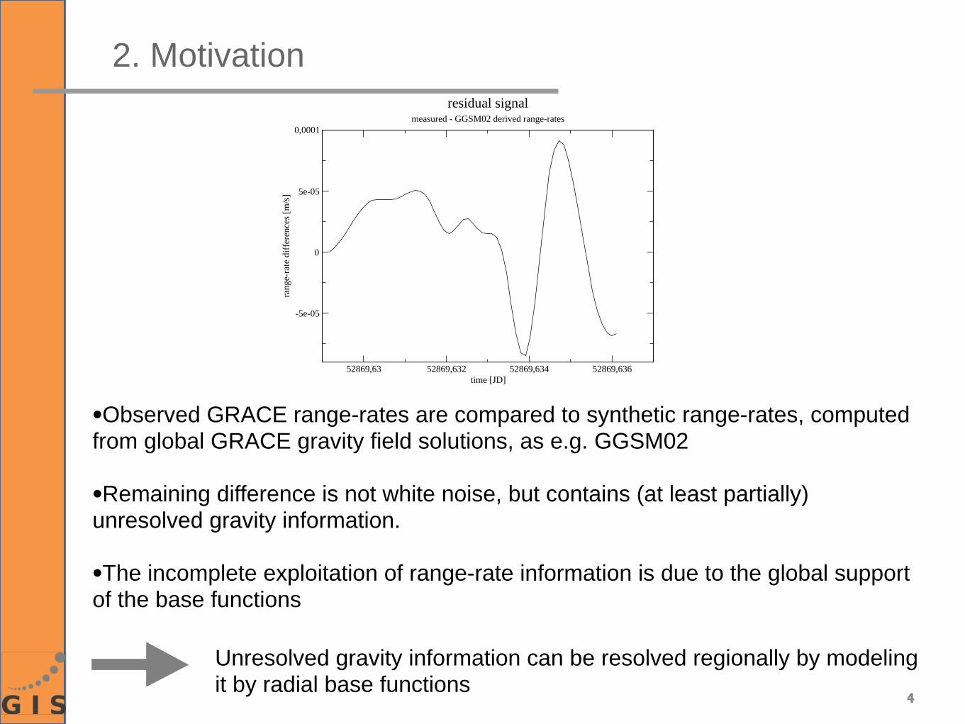
residual signalmeasured - GGSM02 derived range-rates
4
2. Motivation
•Observed GRACE range-rates are compared to synthetic range-rates, computed from global GRACE gravity field solutions, as e.g. GGSM02
•Remaining difference is not white noise, but contains (at least partially) unresolved gravity information.
•The incomplete exploitation of range-rate information is due to the global support of the base functions
Unresolved gravity information can be resolved regionally by modeling it by radial base functions
5
1. Motivation (cont.)
6
1. Motivation (cont.)
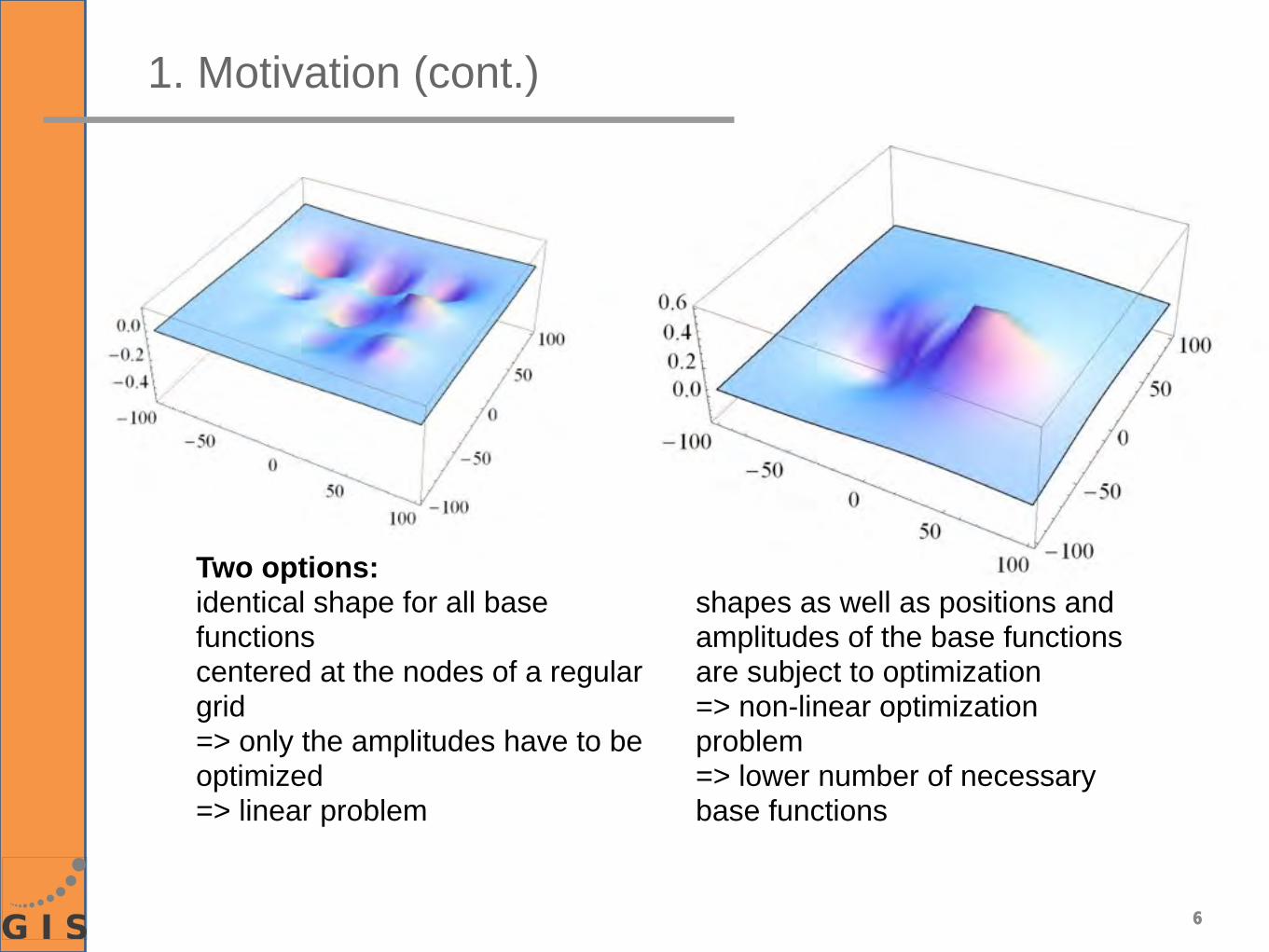
Two options:identical shape for all base functionscentered at the nodes of a regular grid=> only the amplitudes have to be optimized=> linear problem
shapes as well as positions and amplitudes of the base functions are subject to optimization=> non-linear optimization problem=> lower number of necessary base functions
7
3. Radial base functions
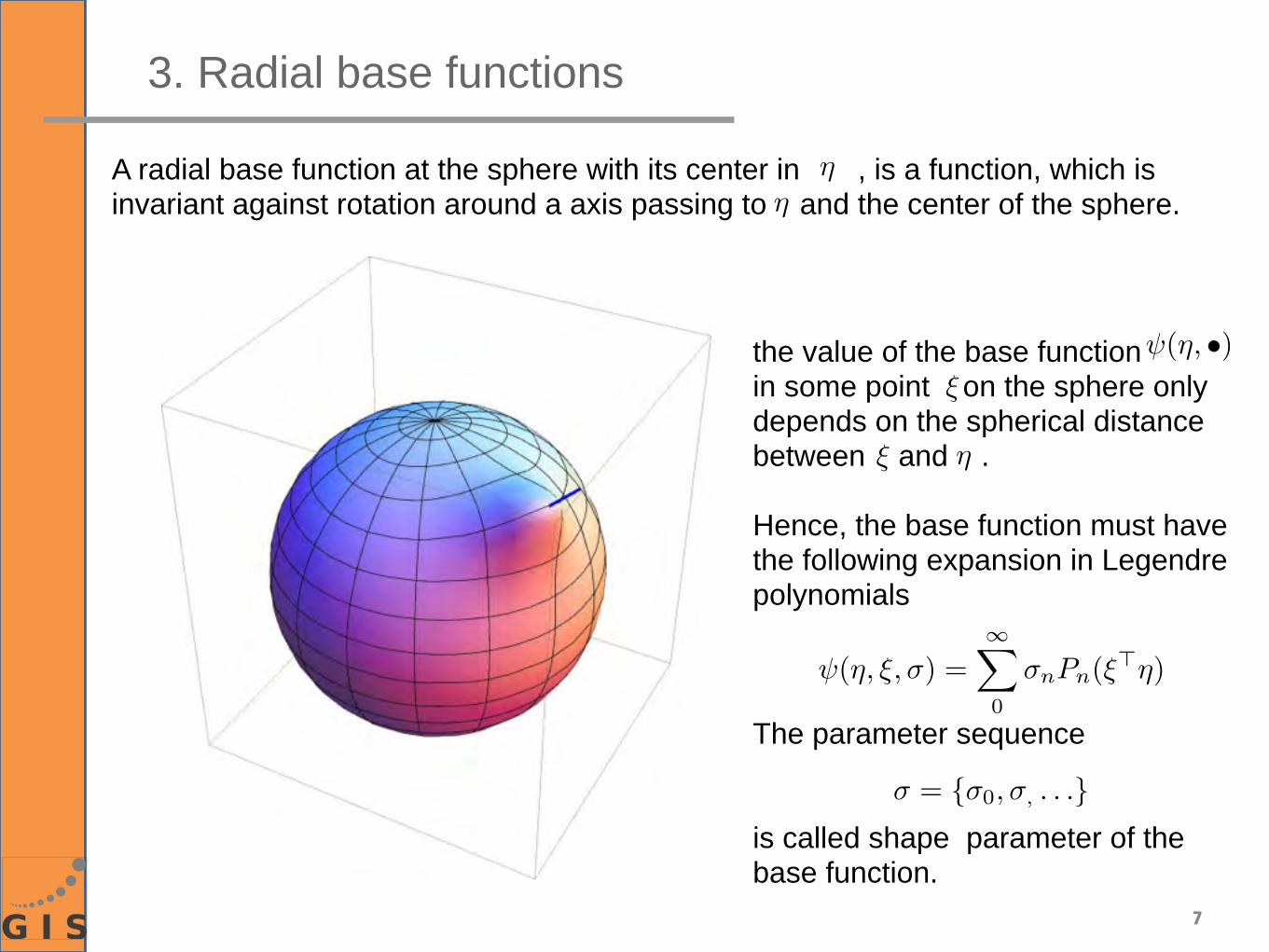
A radial base function at the sphere with its center in , is a function, which is invariant against rotation around a axis passing to and the center of the sphere.
⌘⌘
the value of the base function in some point on the sphere only depends on the spherical distance between and .
Hence, the base function must have the following expansion in Legendre polynomials
The parameter sequence
is called shape parameter of the base function.
⌘
⇠
⇠
⇥(�, •)
⌅(�, ⇥,⇤) =1X
0
⇤nPn(⇥>�)
� = {�0, �, . . .}
8
3. Radial base functions (cont.)
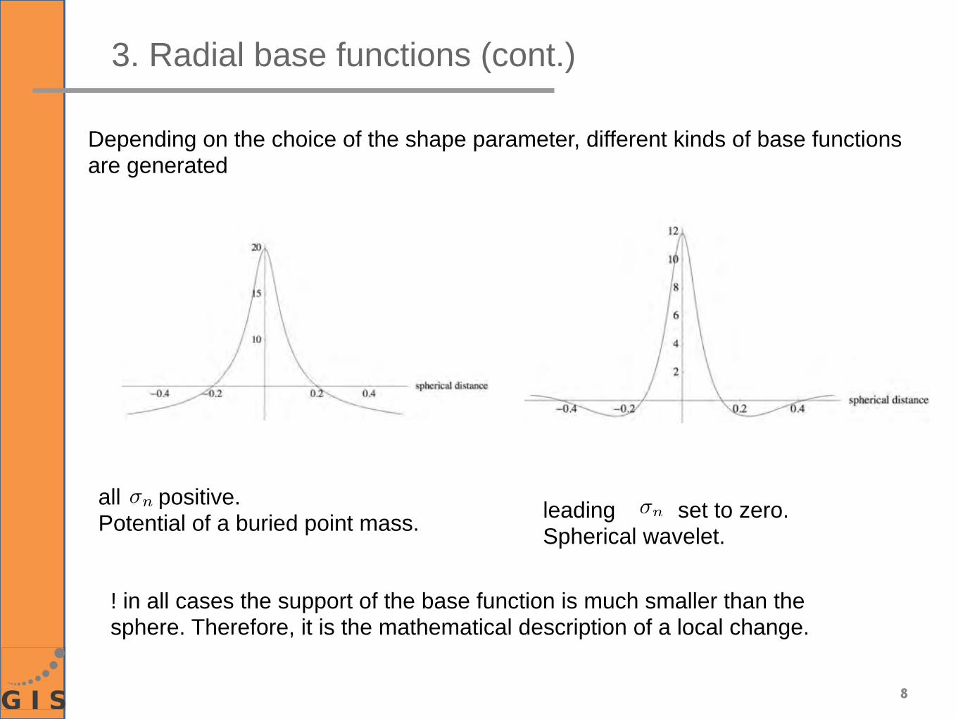
Depending on the choice of the shape parameter, different kinds of base functions are generated
all positive.Potential of a buried point mass. leading set to zero.
Spherical wavelet.
�n �n
! in all cases the support of the base function is much smaller than the sphere. Therefore, it is the mathematical description of a local change.
⇤Y � F(x)⇤2 ⇥ min
Y = (⇥(t1), . . . , ⇥(tN ))>, F(x) = (⇥synth(t1, cj , ⇤j , �j), . . . , ⇥synth(tN , cj , ⇤j , �j))>
⇢synth = ⇢synth(t, cj , �j , ⌘j) =(x2,synth � x1,synth)>(x2,synth � x1,synth)
kx2,synth � x1,synthk
V = V0 + �V = V0 +X
j
cj (⌘j , ⇠,�j)
9
4. Non-linear optimization
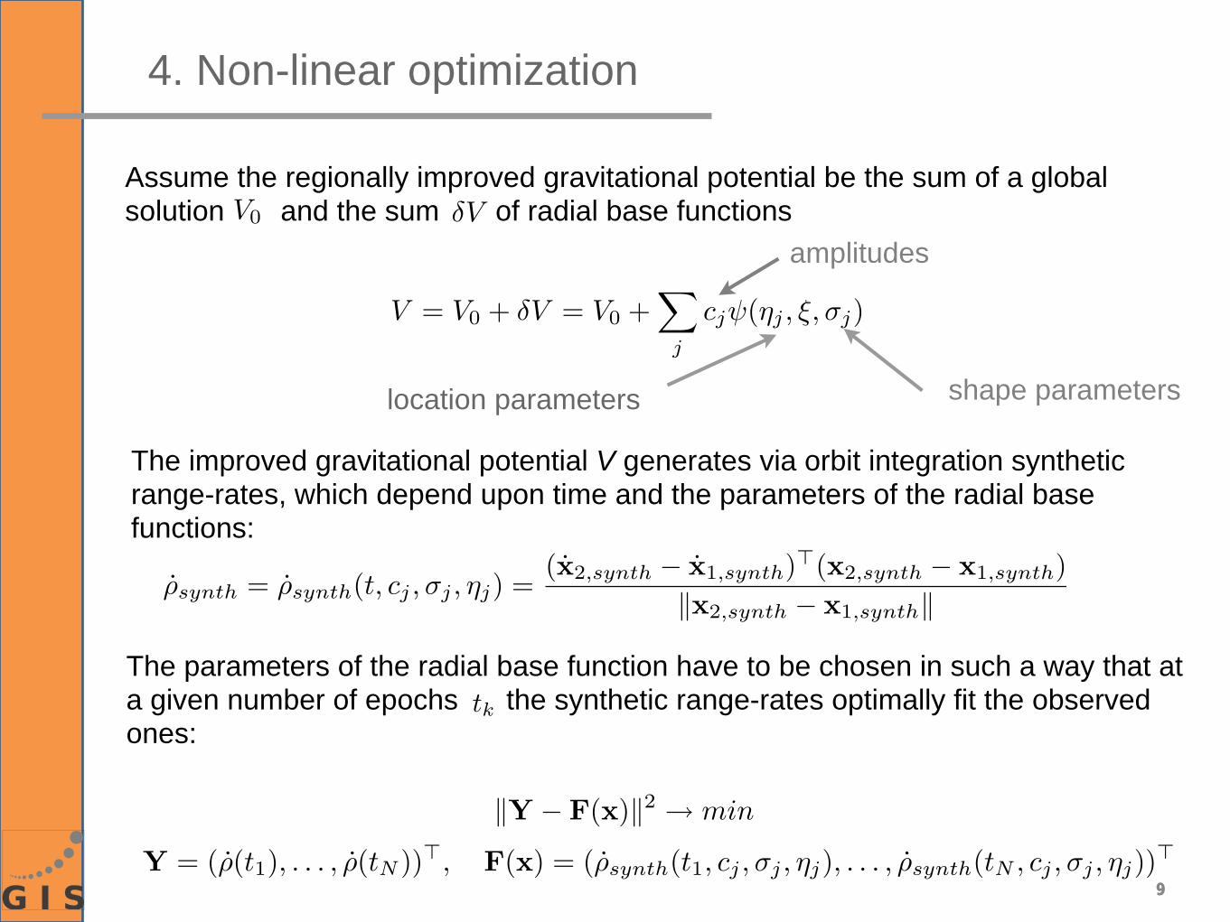
Assume the regionally improved gravitational potential be the sum of a global solution and the sum of radial base functions V0 �V
amplitudes
shape parameterslocation parameters
The improved gravitational potential V generates via orbit integration synthetic range-rates, which depend upon time and the parameters of the radial base functions:
The parameters of the radial base function have to be chosen in such a way that at a given number of epochs the synthetic range-rates optimally fit the observed ones:
tk
F �(xn) =
�
⇧⇧⇧⇧⇤
⇤⇥c1
(t1) . . . ⇤⇥�N
(t1)⇤⇥c1
(t2) . . . ⇤⇥�N
(t2)...
⇤⇥c1
(tM ) . . . ⇤⇥�N
(tM )
⇥
⌃⌃⌃⌃⌅
⇧⇥
⇧p=
⇧⇥
⇧x
⇧x
⇧p+
⇧⇥
⇧x
⇧x
⇧p, p � {c1, . . . , �N}
⇥ �⇥2V0⇥ = ⇥�V, ⇥ =⌅x
⌅p
10
4. Non-linear optimization (cont.)
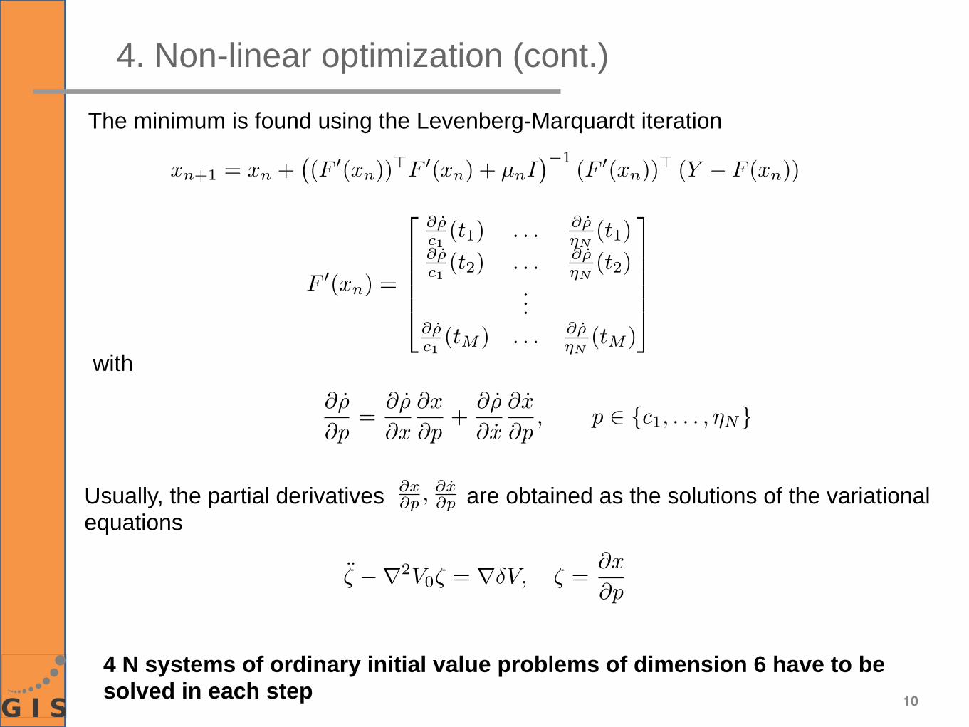
with
Usually, the partial derivatives are obtained as the solutions of the variational equations
�x�p , �x
�p
4 N systems of ordinary initial value problems of dimension 6 have to be solved in each step
The minimum is found using the Levenberg-Marquardt iteration
xn+1 = xn +�(F ⇥(xn))⇤F ⇥(xn) + µnI
⇥�1(F ⇥(xn))⇤ (Y � F (xn))
11
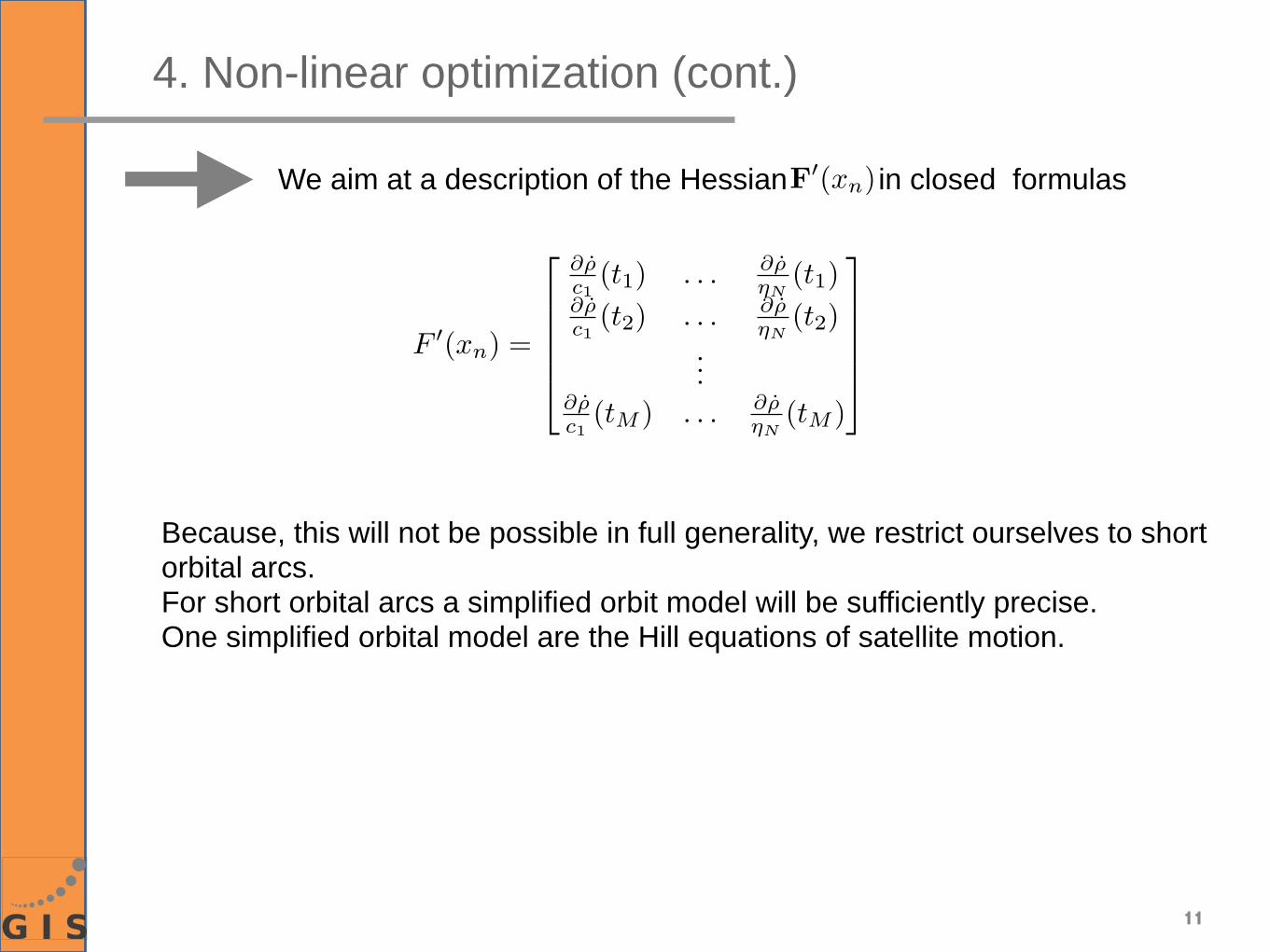
4. Non-linear optimization (cont.)
We aim at a description of the Hessian in closed formulasF0(xn)
F �(xn) =
�
⇧⇧⇧⇧⇤
⇤⇥c1
(t1) . . . ⇤⇥�N
(t1)⇤⇥c1
(t2) . . . ⇤⇥�N
(t2)...
⇤⇥c1
(tM ) . . . ⇤⇥�N
(tM )
⇥
⌃⌃⌃⌃⌅
Because, this will not be possible in full generality, we restrict ourselves to shortorbital arcs. For short orbital arcs a simplified orbit model will be sufficiently precise. One simplified orbital model are the Hill equations of satellite motion.
12
5. Hill equations
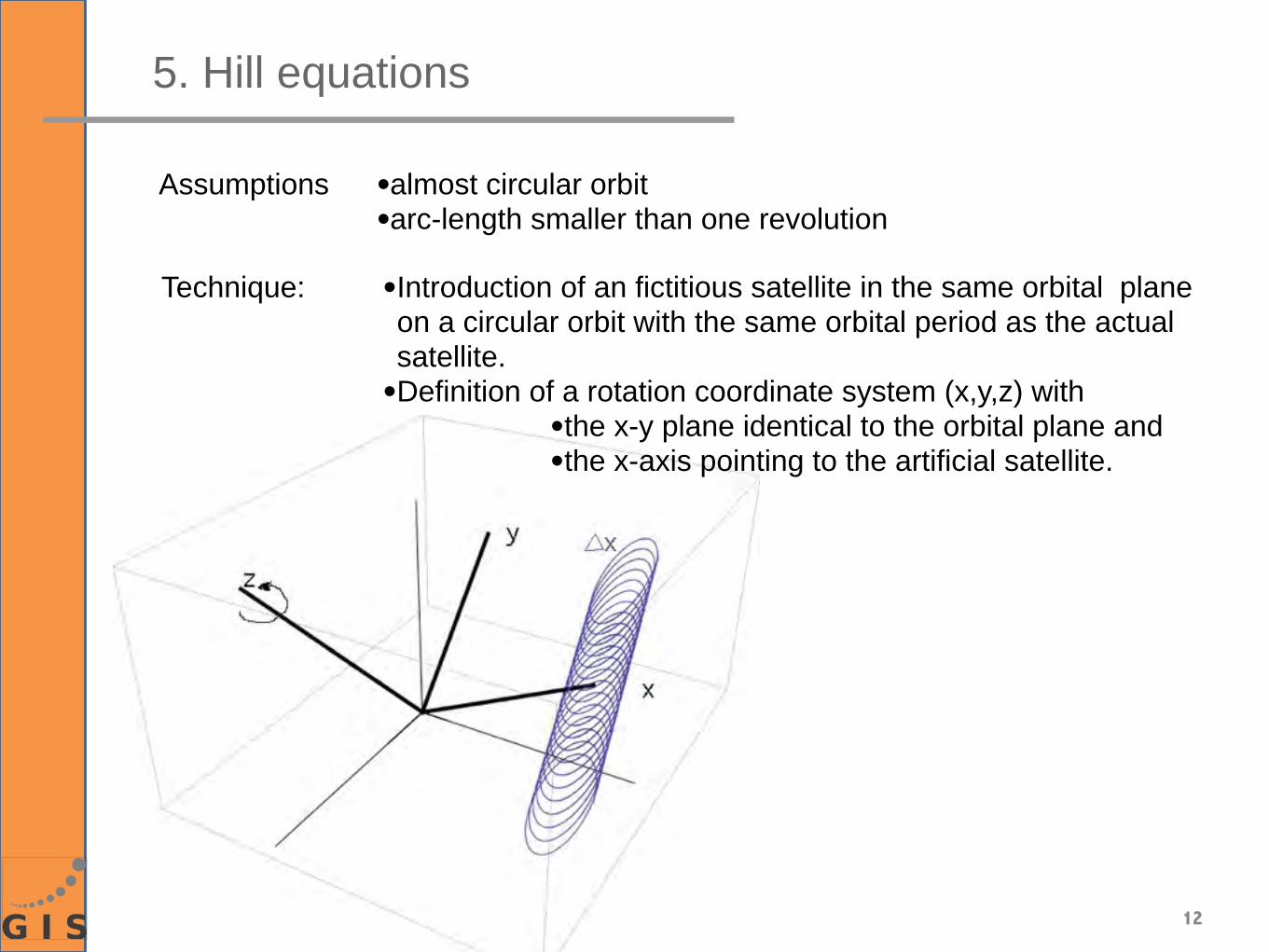
Assumptions •almost circular orbit•arc-length smaller than one revolution
Technique: •Introduction of an fictitious satellite in the same orbital plane on a circular orbit with the same orbital period as the actual satellite.
•Definition of a rotation coordinate system (x,y,z) with•the x-y plane identical to the orbital plane and•the x-axis pointing to the artificial satellite.
13
5. Hill equations (cont.)
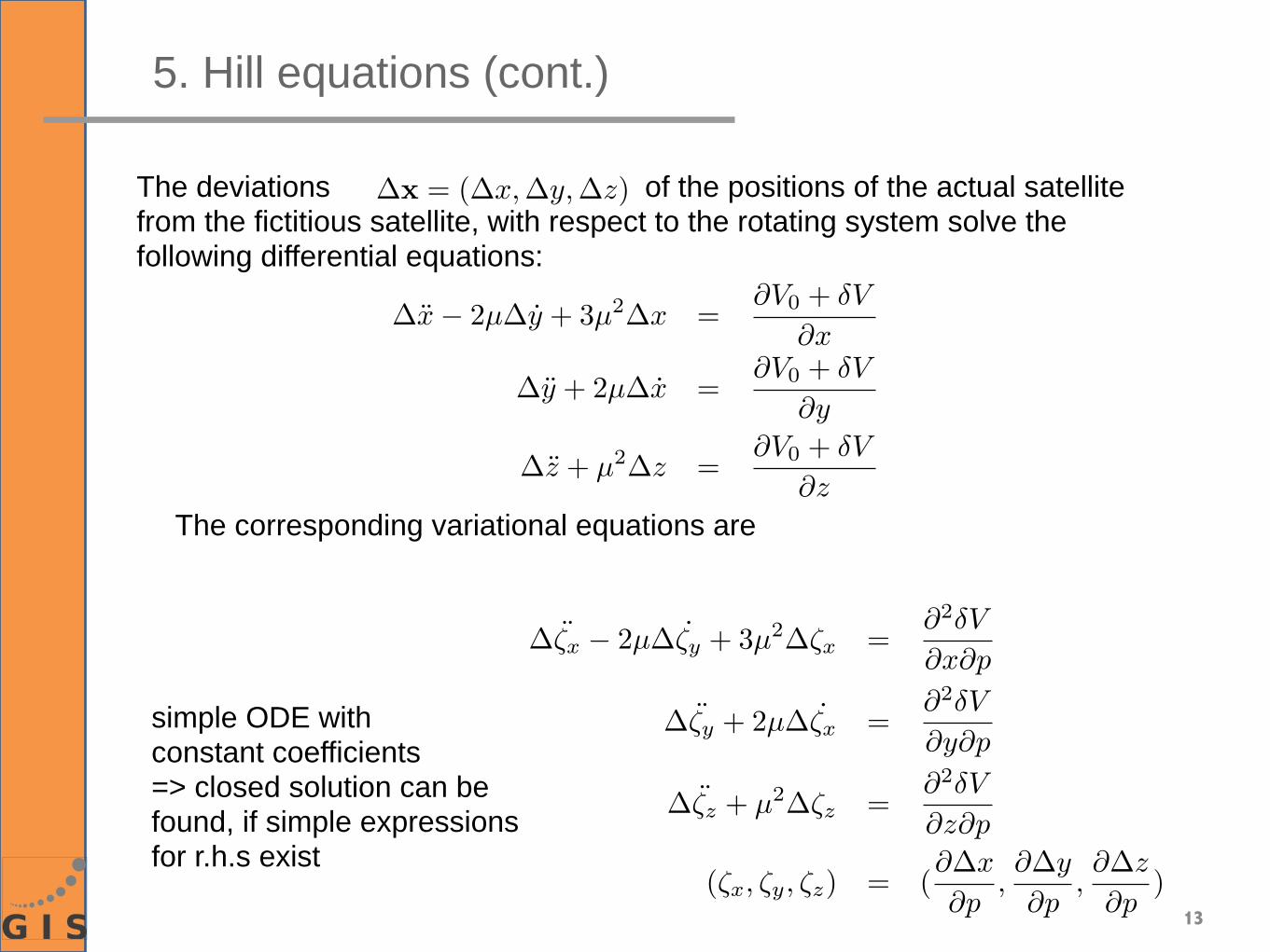
The deviations of the positions of the actual satellite from the fictitious satellite, with respect to the rotating system solve the following differential equations:
�x = (�x,�y, �z)
�x� 2µ�y + 3µ2�x =⇤V0 + �V
⇤x
�y + 2µ�x =⇤V0 + �V
⇤y
�z + µ2�z =⇤V0 + �V
⇤zThe corresponding variational equations are
�⇥x � 2µ�⇥y + 3µ2�⇥x =⇧2�V
⇧x⇧p
�⇥y + 2µ�⇥x =⇧2�V
⇧y⇧p
�⇥z + µ2�⇥z =⇧2�V
⇧z⇧p
(⇥x, ⇥y, ⇥z) = (⇧�x
⇧p,⇧�y
⇧p,⇧�z
⇧p)
simple ODE with constant coefficients=> closed solution can befound, if simple expressionsfor r.h.s exist
�⇥x � 2µ�⇥y + 3µ2�⇥x =⇧2�V
⇧x⇧p
�⇥y + 2µ�⇥x =⇧2�V
⇧y⇧p
�⇥z + µ2�⇥z =⇧2�V
⇧z⇧p
(⇥x, ⇥y, ⇥z) = (⇧�x
⇧p,⇧�y
⇧p,⇧�z
⇧p)
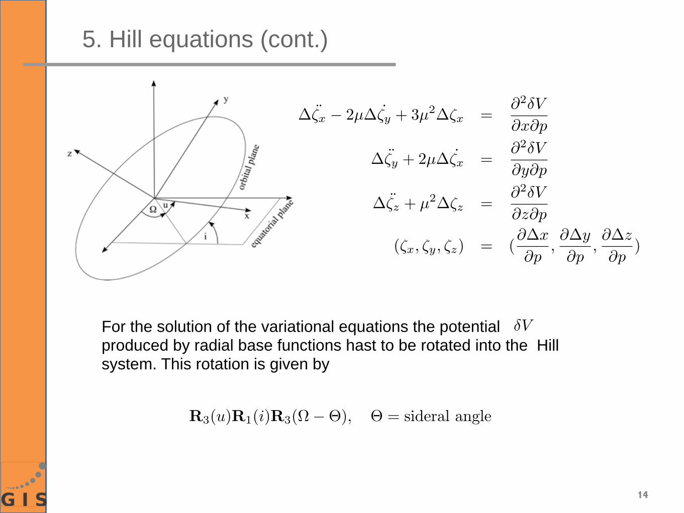
R3(u)R1(i)R3(⇥��), � = sideral angle
14
For the solution of the variational equations the potential produced by radial base functions hast to be rotated into the Hill system. This rotation is given by
�V
5. Hill equations (cont.)
Y l,m(⌅0, ⇧0) =lX
k=�l
Dlk,m(�,⇥, ⇤)Y l,k(⌅,⇧)
15
6. SO(3) group
Y l,m(�,⇥)Y l,m(�0, ⇥0)
Dlk,m(�,⇥, ⇤)
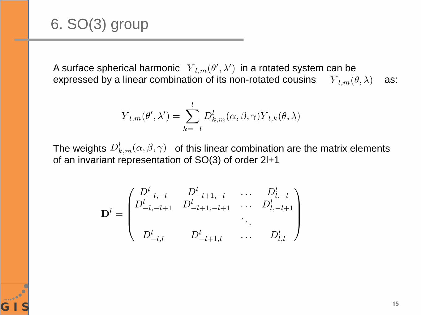
A surface spherical harmonic in a rotated system can be expressed by a linear combination of its non-rotated cousins as:
The weights of this linear combination are the matrix elements of an invariant representation of SO(3) of order 2l+1
Dl =
0
BBB@
Dl�l,�l Dl
�l+1,�l . . . Dll,�l
Dl�l,�l+1 Dl
�l+1,�l+1 . . . Dll,�l+1
. . .Dl�l,l Dl
�l+1,l . . . Dll,l
1
CCCA
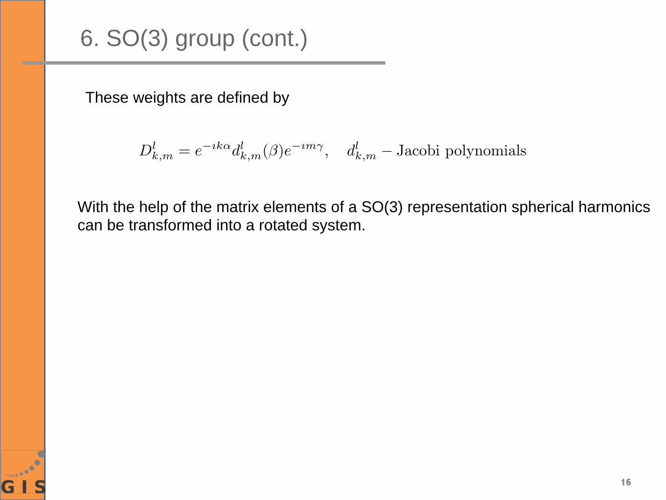
Dlk,m = e�ık�dl
k,m(�)e�ım⇥ , dlk,m � Jacobi polynomials
16
6. SO(3) group (cont.)
With the help of the matrix elements of a SO(3) representation spherical harmonicscan be transformed into a rotated system.
These weights are defined by
⇤(⇥, �, x) =�
n�N
⇥nPn(�⇥x)
⌅(⇤, �, x) =�
n⇥N
⇤n 4⇥
2n + 1
n�
m=�n
Yn,m(�)Yn,m(x)
17
7. Radial base functions in Hill System
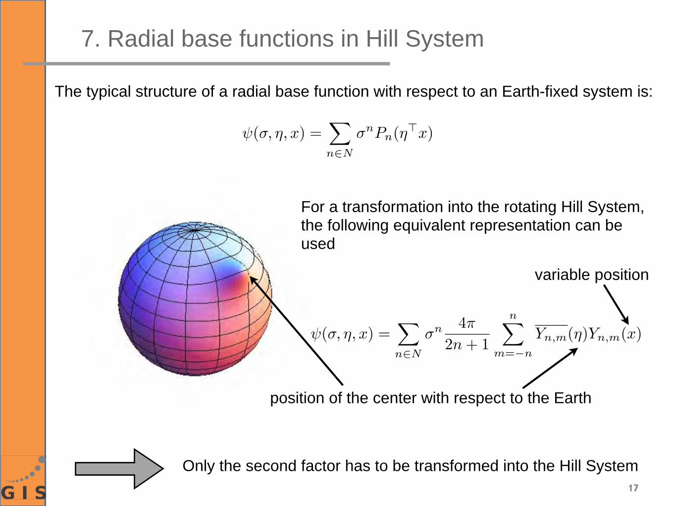
The typical structure of a radial base function with respect to an Earth-fixed system is:
For a transformation into the rotating Hill System, the following equivalent representation can be used
position of the center with respect to the Earth
variable position
Only the second factor has to be transformed into the Hill System
Yn,m(x) =n�
k=�n
dnk,m(i)eı((k�m) �
2 +m⇥)Yn,k(�
2, 0)
⌅ ⇤⇥ ⇧constant
· eı(ku�m�)⌅ ⇤⇥ ⇧
periodic
⌅(⇤, �, x) =⇥�
n=0
n�
m=�n
n�
k=�n
4⇥⇤n
2n + 1Yn,m(�)dn
k,m(i)eı((k�m) �2 +m⇥)Yn,k(
⇥
2, 0)
⌅ ⇤⇥ ⇧=:An,m,k
· eı(ku�m�)⌅ ⇤⇥ ⇧
periodic
=⇥�
n=0
n�
m=�n
n�
k=�n
An,m,keı(ku�m�)
18
6. Radial base functions in Hill System (cont.)
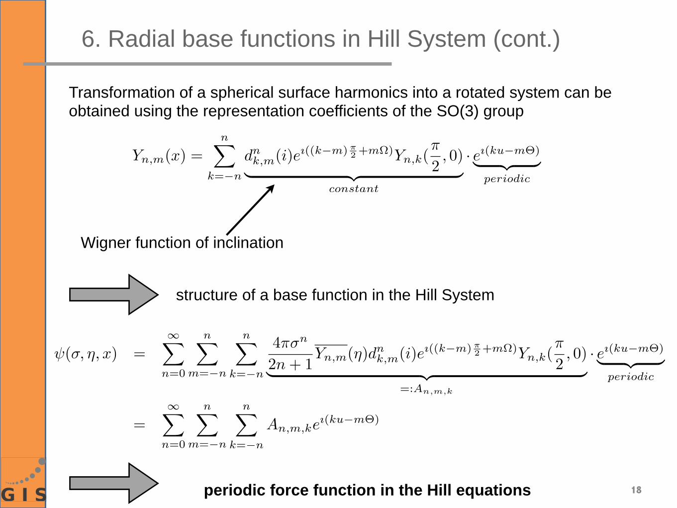
Transformation of a spherical surface harmonics into a rotated system can be obtained using the representation coefficients of the SO(3) group
Wigner function of inclination
structure of a base function in the Hill System
periodic force function in the Hill equations
�⇥x � 2µ�⇥y + 3µ2�⇥x =⇤2�V
⇤x⇤p
�⇥y + 2µ�⇥x =⇤2�V
⇤y⇤p
�⇥z + µ2�⇥z =⇤2�V
⇤z⇤p
(⇥x, ⇥y, ⇥z) = (⇤�x
⇤p,⇤�y
⇤p,⇤�z
⇤p)
�
⇧⇤
⇤2�V⇤x⇤p⇤2�V⇤y⇤p⇤2�V⇤z⇤p
⇥
⌃⌅ =⌥
j
⌥
n
⌥
m
⌥
k
cj
�
⇤Ax
n,m,k
Ayn,m,k
Azn,m,k
⇥
⌅ · eı(ku�m�)
19
7. Closed solution of variational equations in Hill system
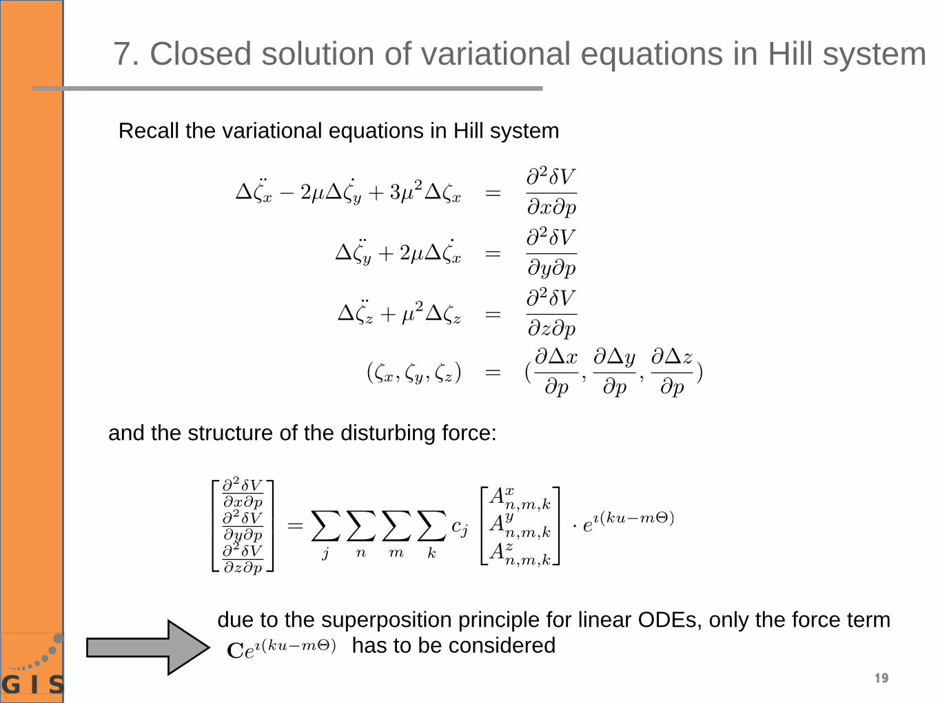
Recall the variational equations in Hill system
and the structure of the disturbing force:
due to the superposition principle for linear ODEs, only the force term has to be consideredCeı(ku�m�)
��x � 2µ��y + 3µ2��x = Cxeı(ku�m�)
��y + 2µ��x = Cyeı(ku�m�)
��z + µ2��z = Czeı(ku�m�)
20
7. Closed solution of variational equations in Hill system
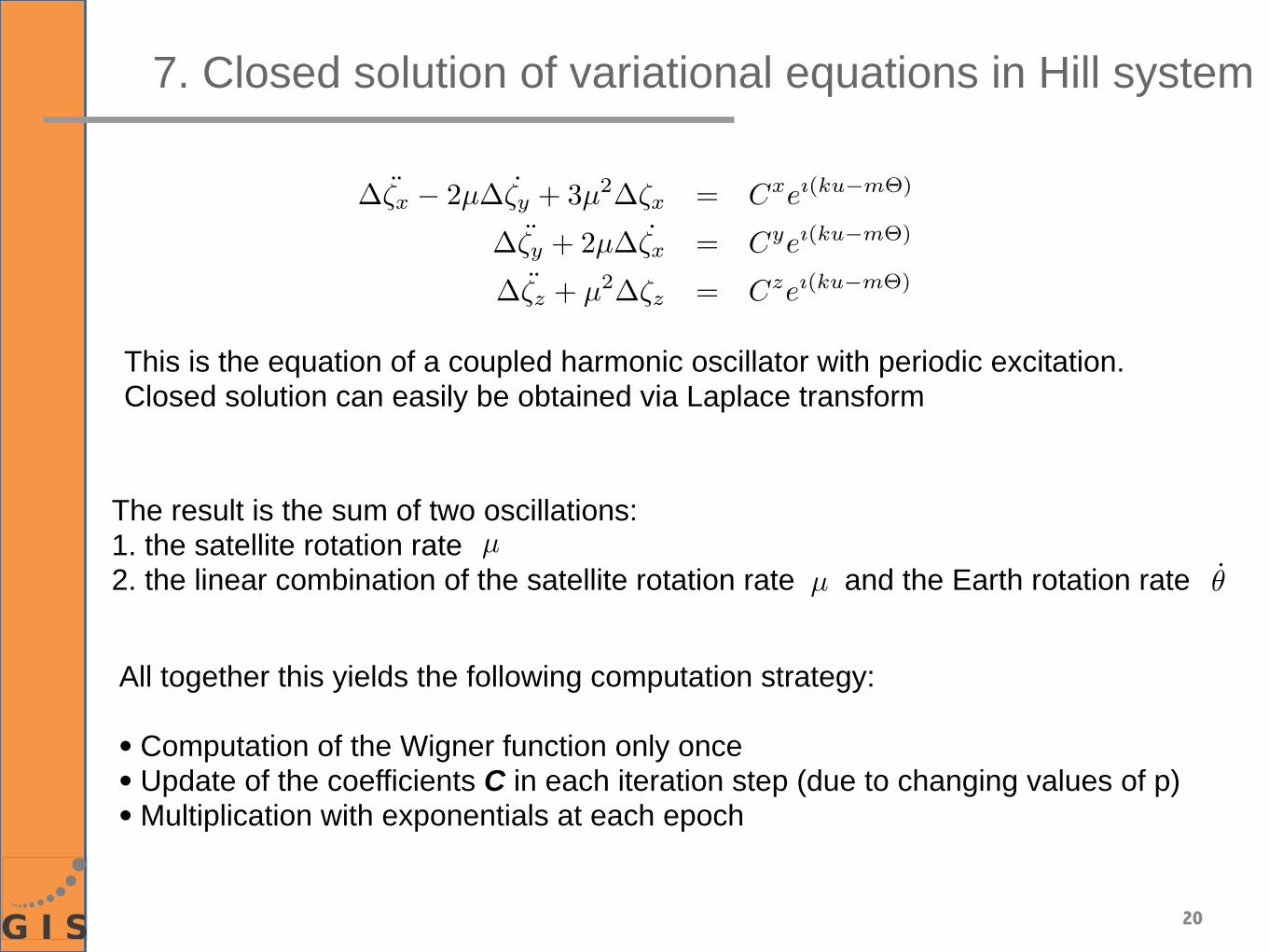
This is the equation of a coupled harmonic oscillator with periodic excitation. Closed solution can easily be obtained via Laplace transform
The result is the sum of two oscillations:1. the satellite rotation rate2. the linear combination of the satellite rotation rate and the Earth rotation rate
µµ �
All together this yields the following computation strategy:
• Computation of the Wigner function only once• Update of the coefficients C in each iteration step (due to changing values of p)• Multiplication with exponentials at each epoch
21
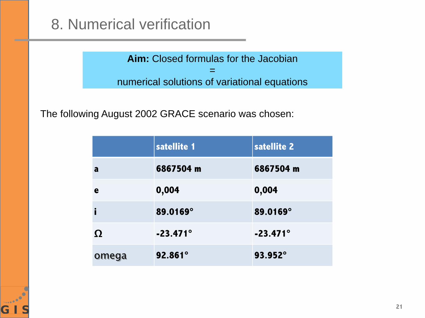
8. Numerical verification
Aim: Closed formulas for the Jacobian =
numerical solutions of variational equations
The following August 2002 GRACE scenario was chosen:
satellite 1 satellite 2
a 6867504 m 6867504 m
e 0,004 0,004
i 89.0169° 89.0169°
Ω -23.471° -23.471°
omega 92.861° 93.952°
22
8. Numerical verification (cont.)
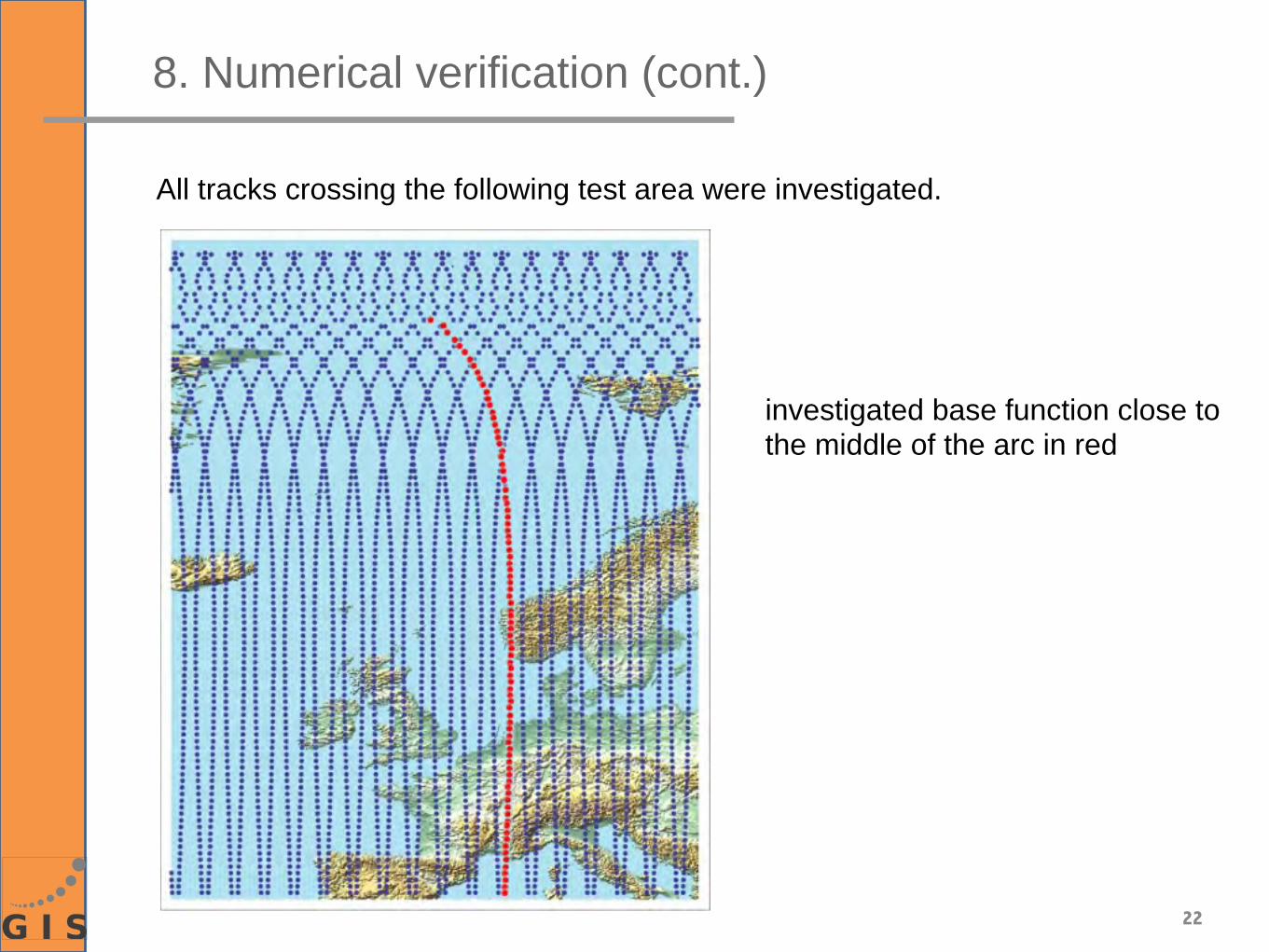
All tracks crossing the following test area were investigated.
investigated base function close to the middle of the arc in red
23
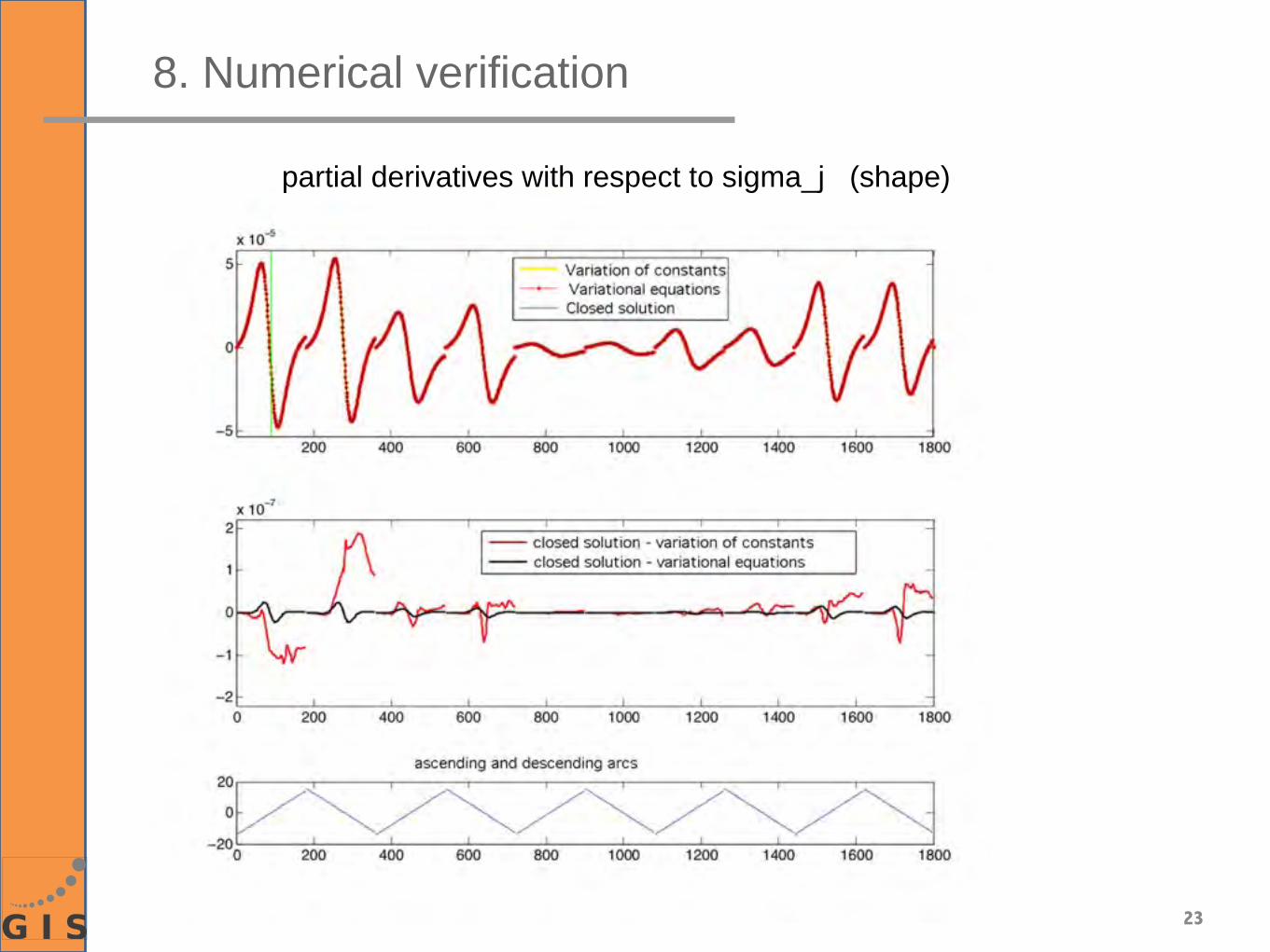
8. Numerical verification
partial derivatives with respect to sigma_j (shape)
24
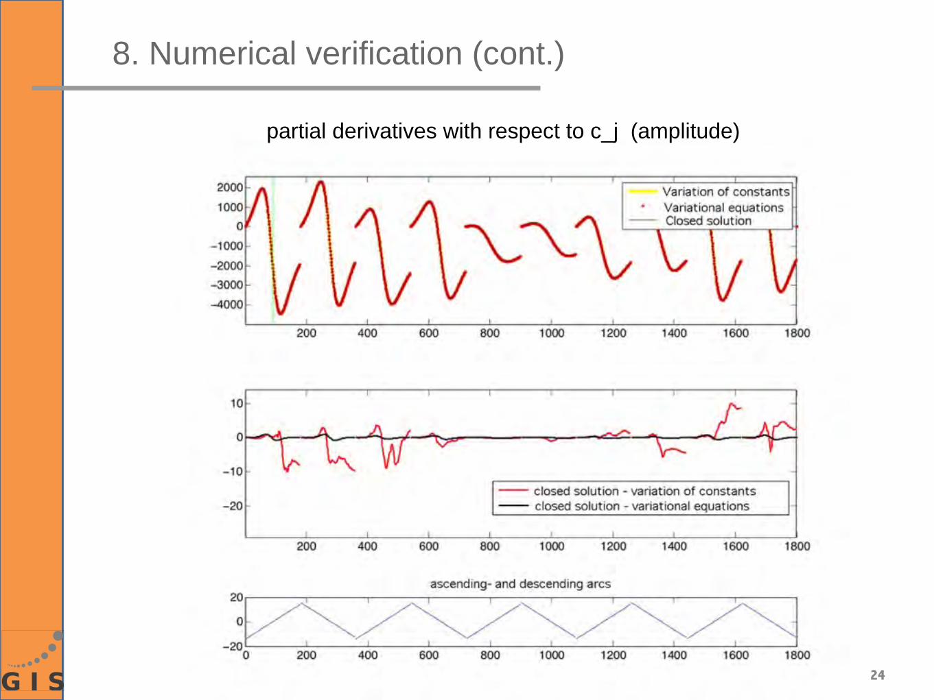
8. Numerical verification (cont.)
partial derivatives with respect to c_j (amplitude)
25
8. Numerical verification (cont.)
Using the closed solution for the variational equations, a small-scale simulation study was carried out. It consisted of four steps:
1. Three radial base functions were randomly chosen. (All parameters randomly). These base function were superimposed the GGM02 field.
2.The orbits of the two GRACE satellites and the resulting range rates were computed in this combined field.
3. The same procedure was repeated for the GGM02 field alone.
4.From the residual range rates the parameters of the base functions were estimated, using non-linear optimization techniques
26
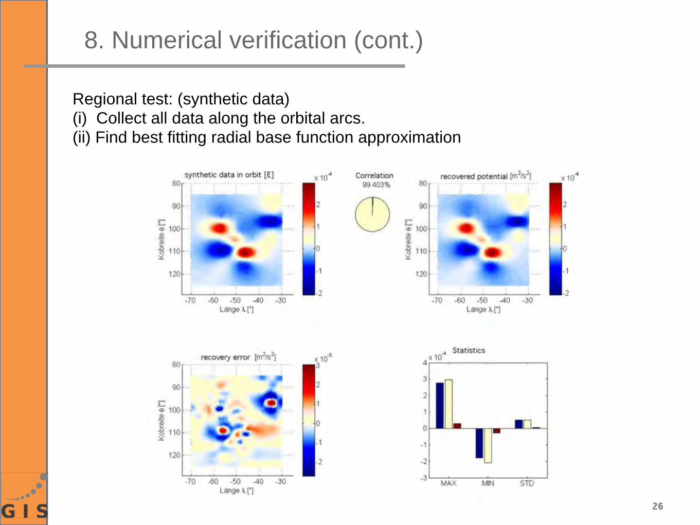
8. Numerical verification (cont.)
Regional test: (synthetic data) (i) Collect all data along the orbital arcs. (ii) Find best fitting radial base function approximation
27
8. Numerical verification (cont.)
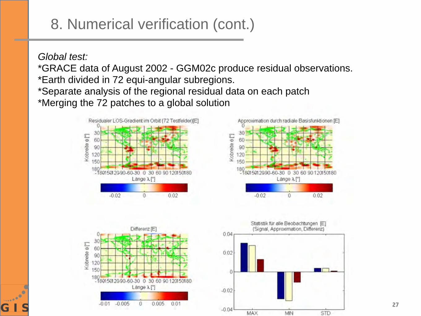
Global test:*GRACE data of August 2002 - GGM02c produce residual observations.*Earth divided in 72 equi-angular subregions.*Separate analysis of the regional residual data on each patch*Merging the 72 patches to a global solution
28
9. Summary
• approximation of a residual potential by radial base functions with variable sizes and position leads to a non-linear optimization problem
• iterative solution of the non-linear optimization problem requires the computation of the partial derivatives in each step
• the usual computation via variational equation is computational demanding
• an arc-wise treatment in a rotating Hill system leads to variational equations which can be solved in a closed form
• the feasibility of regional gravity field improvement via the closed solution was demonstrated
• further examples for•energy-balance approach•line-of-sight gradiometry•satellite-to-satellite tracking•gradiometry
can be found in the PhD thesis of M. Antoni.