Embed Size (px)
Citation preview
SAS/STAT® 9.2 User’s GuideThe PROBIT Procedure(Book Excerpt)
SAS® Documentation
This document is an individual chapter from SAS/STAT® 9.2 User’s Guide.
The correct bibliographic citation for the complete manual is as follows: SAS Institute Inc. 2008. SAS/STAT® 9.2User’s Guide. Cary, NC: SAS Institute Inc.
Copyright © 2008, SAS Institute Inc., Cary, NC, USA
All rights reserved. Produced in the United States of America.
For a Web download or e-book: Your use of this publication shall be governed by the terms established by the vendorat the time you acquire this publication.
U.S. Government Restricted Rights Notice: Use, duplication, or disclosure of this software and related documentationby the U.S. government is subject to the Agreement with SAS Institute and the restrictions set forth in FAR 52.227-19,Commercial Computer Software-Restricted Rights (June 1987).
SAS Institute Inc., SAS Campus Drive, Cary, North Carolina 27513.
1st electronic book, March 20082nd electronic book, February 2009SAS® Publishing provides a complete selection of books and electronic products to help customers use SAS software toits fullest potential. For more information about our e-books, e-learning products, CDs, and hard-copy books, visit theSAS Publishing Web site at support.sas.com/publishing or call 1-800-727-3228.
SAS® and all other SAS Institute Inc. product or service names are registered trademarks or trademarks of SAS InstituteInc. in the USA and other countries. ® indicates USA registration.
Other brand and product names are registered trademarks or trademarks of their respective companies.
Chapter 71
The PROBIT Procedure
ContentsOverview: PROBIT Procedure . . . . . . . . . . . . . . . . . . . . . . . . . . . . 5252Getting Started: PROBIT Procedure . . . . . . . . . . . . . . . . . . . . . . . . . 5253
Estimating the Natural Response Threshold Parameter . . . . . . . . . . . . 5253Syntax: PROBIT Procedure . . . . . . . . . . . . . . . . . . . . . . . . . . . . . 5257
PROC PROBIT Statement . . . . . . . . . . . . . . . . . . . . . . . . . . . 5258BY Statement . . . . . . . . . . . . . . . . . . . . . . . . . . . . . . . . . 5262CDFPLOT Statement . . . . . . . . . . . . . . . . . . . . . . . . . . . . . 5262CLASS Statement . . . . . . . . . . . . . . . . . . . . . . . . . . . . . . . 5271INSET Statement . . . . . . . . . . . . . . . . . . . . . . . . . . . . . . . . 5271IPPPLOT Statement . . . . . . . . . . . . . . . . . . . . . . . . . . . . . . 5273LPREDPLOT Statement . . . . . . . . . . . . . . . . . . . . . . . . . . . . 5281MODEL Statement . . . . . . . . . . . . . . . . . . . . . . . . . . . . . . . 5289OUTPUT Statement . . . . . . . . . . . . . . . . . . . . . . . . . . . . . . 5293PREDPPLOT Statement . . . . . . . . . . . . . . . . . . . . . . . . . . . . 5294WEIGHT Statement . . . . . . . . . . . . . . . . . . . . . . . . . . . . . . 5303
Details: PROBIT Procedure . . . . . . . . . . . . . . . . . . . . . . . . . . . . . 5303Missing Values . . . . . . . . . . . . . . . . . . . . . . . . . . . . . . . . . 5303Response Level Ordering . . . . . . . . . . . . . . . . . . . . . . . . . . . 5303Computational Method . . . . . . . . . . . . . . . . . . . . . . . . . . . . . 5304Distributions . . . . . . . . . . . . . . . . . . . . . . . . . . . . . . . . . . 5305INEST= SAS-data-set . . . . . . . . . . . . . . . . . . . . . . . . . . . . . 5306Model Specification . . . . . . . . . . . . . . . . . . . . . . . . . . . . . . 5307Lack-of-Fit Tests . . . . . . . . . . . . . . . . . . . . . . . . . . . . . . . . 5307Rescaling the Covariance Matrix . . . . . . . . . . . . . . . . . . . . . . . 5308Tolerance Distribution . . . . . . . . . . . . . . . . . . . . . . . . . . . . . 5309Inverse Confidence Limits . . . . . . . . . . . . . . . . . . . . . . . . . . . 5309OUTEST= SAS-data-set . . . . . . . . . . . . . . . . . . . . . . . . . . . 5310XDATA= SAS-data-set . . . . . . . . . . . . . . . . . . . . . . . . . . . . 5311Traditional High-Resolution Graphics . . . . . . . . . . . . . . . . . . . . . 5312Displayed Output . . . . . . . . . . . . . . . . . . . . . . . . . . . . . . . . 5317ODS Table Names . . . . . . . . . . . . . . . . . . . . . . . . . . . . . . . 5318ODS Graphics . . . . . . . . . . . . . . . . . . . . . . . . . . . . . . . . . 5319
Examples: PROBIT Procedure . . . . . . . . . . . . . . . . . . . . . . . . . . . . 5323Example 71.1: Dosage Levels . . . . . . . . . . . . . . . . . . . . . . . . . 5323
5252 F Chapter 71: The PROBIT Procedure
Example 71.2: Multilevel Response . . . . . . . . . . . . . . . . . . . . . . 5331Example 71.3: Logistic Regression . . . . . . . . . . . . . . . . . . . . . . 5337Example 71.4: An Epidemiology Study . . . . . . . . . . . . . . . . . . . . 5339
References . . . . . . . . . . . . . . . . . . . . . . . . . . . . . . . . . . . . . . 5350
Overview: PROBIT Procedure
The PROBIT procedure calculates maximum likelihood estimates of regression parameters and thenatural (or threshold) response rate for quantal response data from biological assays or other discreteevent data. This includes probit, logit, ordinal logistic, and extreme value (or gompit) regressionmodels.
Probit analysis developed from the need to analyze qualitative (dichotomous or polytomous) de-pendent variables within the regression framework. Many response variables are binary by nature(yes/no), while others are measured ordinally rather than continuously (degree of severity). Collett(1991) and Agresti (1990), for example, have shown ordinary least squares (OLS) regression to beinadequate when the dependent variable is discrete. Probit or logit analyses are more appropriate inthis case.
The PROBIT procedure computes maximum likelihood estimates of the parameters ˇ and C of theprobit equation by using a modified Newton-Raphson algorithm. When the response Y is binary,with values 0 and 1, the probit equation is
p D Pr.Y D 0/ D C C .1 � C /F.x0ˇ/
where
ˇ is a vector of parameter estimates
F is a cumulative distribution function (normal, logistic, or extreme value)
x is a vector of explanatory variables
p is the probability of a response
C is the natural (threshold) response rate
Notice that PROC PROBIT, by default, models the probability of the lower response levels. Thechoice of the distribution function F (normal for the probit model, logistic for the logit model,and extreme value or Gompertz for the gompit model) determines the type of analysis. For mostproblems, there is relatively little difference between the normal and logistic specifications of themodel. Both distributions are symmetric about the value zero. The extreme value (or Gompertz)distribution, however, is not symmetric, approaching 0 on the left more slowly than it approaches 1on the right. You can use the extreme value distribution where such asymmetry is appropriate.
For ordinal response models, the response, Y, of an individual or an experimental unit can be re-stricted to one of a (usually small) number, kC1.k � 1/, of ordinal values, denoted for convenienceby 1; : : : ; k; kC1. For example, the severity of coronary disease can be classified into three response
Getting Started: PROBIT Procedure F 5253
categories as 1=no disease, 2=angina pectoris, and 3=myocardial infraction. The PROBIT proce-dure fits a common slopes cumulative model, which is a parallel-lines regression model based onthe cumulative probabilities of the response categories rather than on their individual probabilities.The cumulative model has the form
Pr.Y � 1 j x/ D F.x0ˇ/
Pr.Y � i j x/ D F.˛i C x0ˇ/; 2 � i � k
where ˛2; : : : ; ˛k are k � 1 intercept parameters. By default, the covariate vector x contains anoverall intercept term.
You can set or estimate the natural (threshold) response rate C . Estimation of C can begin eitherfrom an initial value that you specify or from the rate observed in a control group. By default, thenatural response rate is fixed at zero.
An observation in the data set analyzed by the PROBIT procedure might contain the response andexplanatory values for one subject. Alternatively, it might provide the number of observed eventsfrom a number of subjects at a particular setting of the explanatory variables. In this case, PROCPROBIT models the probability of an event.
The PROBIT procedure now uses ODS Graphics to create graphs as part of its output. For generalinformation about ODS Graphics, see Chapter 21, “Statistical Graphics Using ODS.”
Getting Started: PROBIT Procedure
The following example illustrates how you can use the PROBIT procedure to compute the thresholdresponse rate and regression parameter estimates for quantal response data.
Estimating the Natural Response Threshold Parameter
Suppose you want to test the effect of a drug at 12 dosage levels. You randomly divide 180 subjectsinto 12 groups of 15—one group for each dosage level. You then conduct the experiment and, foreach subject, record the presence or absence of a positive response to the drug. You summarize thedata by counting the number of subjects responding positively in each dose group. Your data set isas follows:
data study;input Dose Respond @@;Number = 15;datalines;
0 3 1.1 4 1.3 4 2.0 3 2.2 5 2.8 43.7 5 3.9 9 4.4 8 4.8 11 5.9 12 6.8 13;run;
5254 F Chapter 71: The PROBIT Procedure
The variable dose represents the amount of drug administered. The first group, receiving a dose levelof 0, is the control group. The variable number represents the number of subjects in each group. Allgroups are equal in size; hence, number has the value 15 for all observations. The variable respondrepresents the number of subjects responding to the associated drug dosage.
You can model the probability of positive response as a function of dosage by using the followingstatements:
ods graphics on;
proc probit data=study log10 optc plots=(predpplot ippplot);model respond/number=dose;output out=new p=p_hat;
run;
ods graphics off;
The DATA= option specifies that PROC PROBIT analyze the SAS data set study. The LOG10option replaces the first continuous independent variable (dose) with its common logarithm. TheOPTC option estimates the natural response rate. When you use the LOG10 option with the OPTCoption, any observations with a dose value less than or equal to zero are used in the estimation as acontrol group.
The PLOTS= option in the PROC PROBIT statement, together with the ODS GRAPHICS state-ment, requests two plots for the estimated probability values and dosage levels. For general in-formation about ODS Graphics, see Chapter 21, “Statistical Graphics Using ODS.” For specificinformation about the graphics available in the PROBIT procedure, see the section “ODS Graph-ics” on page 5319.
The MODEL statement specifies a proportional response by using the variables respond and numberin events/trials syntax. The variable dose is the stimulus or explanatory variable.
The OUTPUT statement creates a new data set, new, that contains all the variables in the originaldata set, and a new variable, p_hat, that represents the predicted probabilities.
The results from this analysis are displayed in the following figures.
Figure 71.1 displays background information about the model fit. Included are the name of the inputdata set, the response variables used, and the number of observations, events, and trials. The lastline in Figure 71.1 shows the final value of the log-likelihood function.
Figure 71.2 displays the table of parameter estimates for the model. The parameter C , which isthe natural response threshold or the proportion of individuals responding at zero dose, is estimatedto be 0.2409. Since both the intercept and the slope coefficient have significant p-values (0.0020,0.0010), you can write the model for
Pr(response) D C C .1 � C /F.x0ˇ/
as
Pr(response) D 0:2409 C 0:7591.ˆ.�4:1439 C 6:2308 � log10 (dose)//
where ˆ is the normal cumulative distribution function.
Estimating the Natural Response Threshold Parameter F 5255
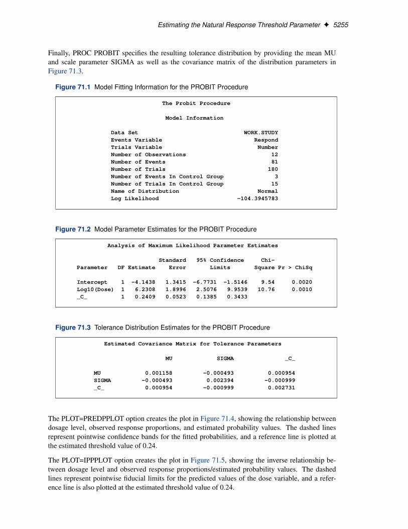
Finally, PROC PROBIT specifies the resulting tolerance distribution by providing the mean MUand scale parameter SIGMA as well as the covariance matrix of the distribution parameters inFigure 71.3.
Figure 71.1 Model Fitting Information for the PROBIT Procedure
The Probit Procedure
Model Information
Data Set WORK.STUDYEvents Variable RespondTrials Variable NumberNumber of Observations 12Number of Events 81Number of Trials 180Number of Events In Control Group 3Number of Trials In Control Group 15Name of Distribution NormalLog Likelihood -104.3945783
Figure 71.2 Model Parameter Estimates for the PROBIT Procedure
Analysis of Maximum Likelihood Parameter Estimates
Standard 95% Confidence Chi-Parameter DF Estimate Error Limits Square Pr > ChiSq
Intercept 1 -4.1438 1.3415 -6.7731 -1.5146 9.54 0.0020Log10(Dose) 1 6.2308 1.8996 2.5076 9.9539 10.76 0.0010_C_ 1 0.2409 0.0523 0.1385 0.3433
Figure 71.3 Tolerance Distribution Estimates for the PROBIT Procedure
Estimated Covariance Matrix for Tolerance Parameters
MU SIGMA _C_
MU 0.001158 -0.000493 0.000954SIGMA -0.000493 0.002394 -0.000999_C_ 0.000954 -0.000999 0.002731
The PLOT=PREDPPLOT option creates the plot in Figure 71.4, showing the relationship betweendosage level, observed response proportions, and estimated probability values. The dashed linesrepresent pointwise confidence bands for the fitted probabilities, and a reference line is plotted atthe estimated threshold value of 0.24.
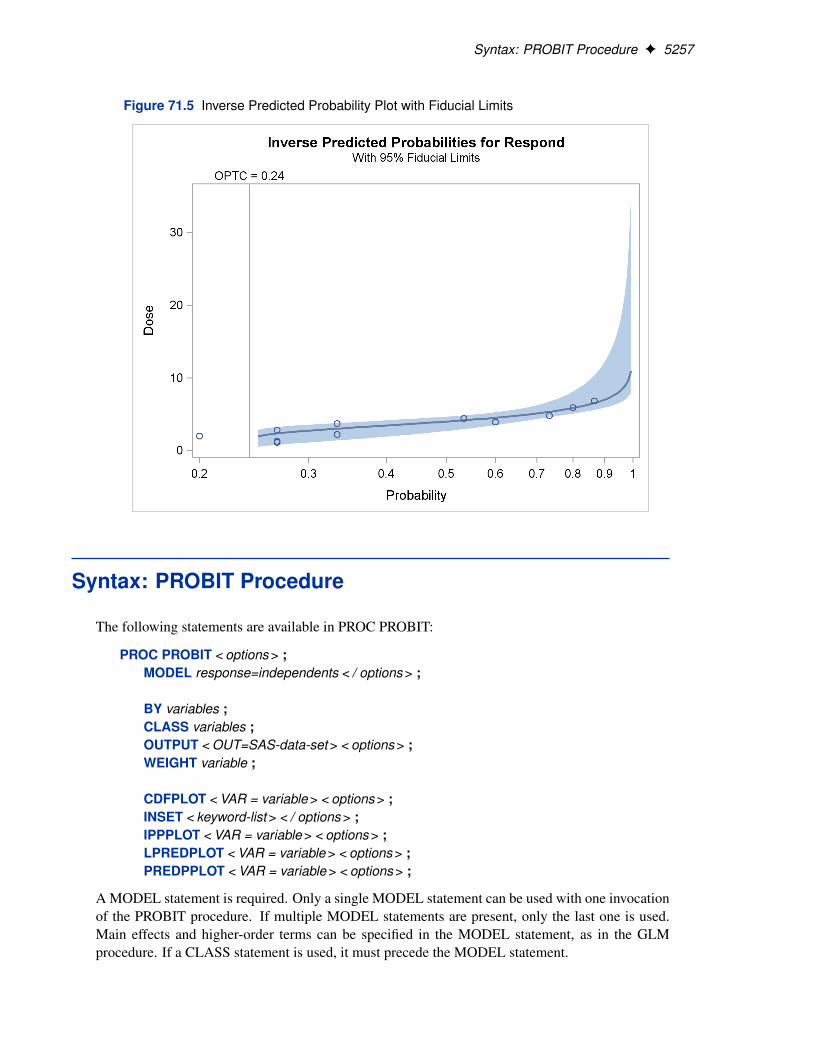
The PLOT=IPPPLOT option creates the plot in Figure 71.5, showing the inverse relationship be-tween dosage level and observed response proportions/estimated probability values. The dashedlines represent pointwise fiducial limits for the predicted values of the dose variable, and a refer-ence line is also plotted at the estimated threshold value of 0.24.

5256 F Chapter 71: The PROBIT Procedure
The two plot options can be put together with the PLOTS= option, as shown in the PROC PROBITstatement.
Figure 71.4 Plot of Observed and Fitted Probabilities versus Dose Level
Syntax: PROBIT Procedure F 5257
Figure 71.5 Inverse Predicted Probability Plot with Fiducial Limits
Syntax: PROBIT Procedure
The following statements are available in PROC PROBIT:
PROC PROBIT < options > ;MODEL response=independents < / options > ;
BY variables ;CLASS variables ;OUTPUT < OUT=SAS-data-set > < options > ;WEIGHT variable ;
CDFPLOT < VAR = variable > < options > ;INSET < keyword-list > < / options > ;IPPPLOT < VAR = variable > < options > ;LPREDPLOT < VAR = variable > < options > ;PREDPPLOT < VAR = variable > < options > ;
A MODEL statement is required. Only a single MODEL statement can be used with one invocationof the PROBIT procedure. If multiple MODEL statements are present, only the last one is used.Main effects and higher-order terms can be specified in the MODEL statement, as in the GLMprocedure. If a CLASS statement is used, it must precede the MODEL statement.
5258 F Chapter 71: The PROBIT Procedure
The CDFPLOT, INSET, IPPPLOT, LPREDPLOT, and PREDPPLOT statements are used to producegraphical output. You can use any appropriate combination of the graphical statements after theMODEL statement.
PROC PROBIT Statement
PROC PROBIT < options > ;
The PROC PROBIT statement starts the procedure. You can specify the following options in thePROC PROBIT statement.
COVOUTwrites the parameter estimate covariance matrix to the OUTEST= data set.
C=rateOPTC
controls how the natural response is handled. Specify the OPTC option to request that thenatural response rate C be estimated. Specify the C=rate option to set the natural responserate or to provide the initial estimate of the natural response rate. The natural response ratevalue must be a number between 0 and 1.
� If you specify neither the OPTC nor the C= option, a natural response rate of zero isassumed.
� If you specify both the OPTC and the C= option, the C= option should be a reasonableinitial estimate of the natural response rate. For example, you could use the ratio of thenumber of responses to the number of subjects in a control group.
� If you specify the C= option but not the OPTC option, the natural response rate is set tothe specified value and not estimated.
� If you specify the OPTC option but not the C= option, PROC PROBIT’s action dependson the response variable, as follows:– If you specify either the LN or LOG10 option and some subjects have the first
independent variable (dose) values less than or equal to zero, these subjects aretreated as a control group. The initial estimate of C is then the ratio of the numberof responses to the number of subjects in this group.
– If you do not specify the LN or LOG10 option or if there is no control group, thenone of the following occurs:� If all responses are greater than zero, the initial estimate of the natural response
rate is the minimal response rate (the ratio of the number of responses to thenumber of subjects in a dose group) across all dose levels.
� If one or more of the responses is zero (making the response rate zero in thatdose group), the initial estimate of the natural rate is the reciprocal of twice thelargest number of subjects in any dose group in the experiment.
DATA=SAS-data-setspecifies the SAS data set to be used by PROC PROBIT. By default, the procedure uses themost recently created SAS data set.
PROC PROBIT Statement F 5259
GOUT=graphics-catalogspecifies a graphics catalog in which to save graphics output.
HPROB=pspecifies a minimum probability level for the Pearson chi-square to indicate a good fit. Thedefault value is 0.10. The LACKFIT option must also be specified for this option to haveany effect. For Pearson goodness-of-fit chi-square values with probability greater than theHPROB= value, the fiducial limits, if requested with the INVERSECL option, are computedby using a critical value of 1.96. For chi-square values with probability less than the valueof the HPROB= option, the critical value is a 0.95 two-sided quantile value taken from the t
distribution with degrees of freedom equal to .k �1/�m�q, where k is the number of levelsfor the response variable, m is the number of different sets of independent variable values,and q is the number of parameters fit in the model. Note that the HPROB= option can alsoappear in the MODEL statement.
INEST=SAS-data-setspecifies an input SAS data set that contains initial estimates for all the parameters in themodel. See the section “INEST= SAS-data-set” on page 5306 for a detailed description ofthe contents of the INEST= data set.
INVERSECLcomputes confidence limits for the values of the first continuous independent variable (suchas dose) that yield selected response rates. If the algorithm fails to converge (this can happenwhen C is nonzero), missing values are reported for the confidence limits. See the section“Inverse Confidence Limits” on page 5309 for details. Note that the INVERSECL option canalso appear in the MODEL statement.
LACKFITperforms two goodness-of-fit tests (a Pearson chi-square test and a log-likelihood ratio chi-square test) for the fitted model.
To compute the test statistics, proper grouping of the observations into subpopulations isneeded. You can use the AGGREGATE or AGGREGATE= option for this end. See the entryfor the AGGREGATE and AGGREGATE= options under the MODEL statement. If neitherAGGREGATE nor AGGREGATE= is specified, PROC PROBIT assumes each observationis from a separate subpopulation and computes the goodness-of-fit test statistics only for theevents/trials syntax.
NOTE: This test is not appropriate if the data are very sparse, with only a few values at eachset of the independent variable values.
If the Pearson chi-square test statistic is significant, then the covariance estimates and stan-dard error estimates are adjusted. See the section “Lack-of-Fit Tests” on page 5307 for adescription of the tests. Note that the LACKFIT option can also appear in the MODEL state-ment.
LOG
LNanalyzes the data by replacing the first continuous independent variable with its natural loga-rithm. This variable is usually the level of some treatment such as dosage. In addition to the
5260 F Chapter 71: The PROBIT Procedure
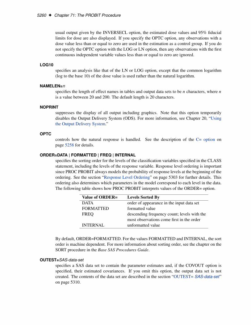
usual output given by the INVERSECL option, the estimated dose values and 95% fiduciallimits for dose are also displayed. If you specify the OPTC option, any observations with adose value less than or equal to zero are used in the estimation as a control group. If you donot specify the OPTC option with the LOG or LN option, then any observations with the firstcontinuous independent variable values less than or equal to zero are ignored.
LOG10specifies an analysis like that of the LN or LOG option, except that the common logarithm(log to the base 10) of the dose value is used rather than the natural logarithm.
NAMELEN=nspecifies the length of effect names in tables and output data sets to be n characters, where n
is a value between 20 and 200. The default length is 20 characters.
NOPRINTsuppresses the display of all output including graphics. Note that this option temporarilydisables the Output Delivery System (ODS). For more information, see Chapter 20, “Usingthe Output Delivery System.”
OPTCcontrols how the natural response is handled. See the description of the C= option onpage 5258 for details.
ORDER=DATA | FORMATTED | FREQ | INTERNALspecifies the sorting order for the levels of the classification variables specified in the CLASSstatement, including the levels of the response variable. Response level ordering is importantsince PROC PROBIT always models the probability of response levels at the beginning of theordering. See the section “Response Level Ordering” on page 5303 for further details. Thisordering also determines which parameters in the model correspond to each level in the data.The following table shows how PROC PROBIT interprets values of the ORDER= option.
Value of ORDER= Levels Sorted ByDATA order of appearance in the input data setFORMATTED formatted valueFREQ descending frequency count; levels with the
most observations come first in the orderINTERNAL unformatted value
By default, ORDER=FORMATTED. For the values FORMATTED and INTERNAL, the sortorder is machine dependent. For more information about sorting order, see the chapter on theSORT procedure in the Base SAS Procedures Guide.
OUTEST=SAS-data-setspecifies a SAS data set to contain the parameter estimates and, if the COVOUT option isspecified, their estimated covariances. If you omit this option, the output data set is notcreated. The contents of the data set are described in the section “OUTEST= SAS-data-set”on page 5310.
PROC PROBIT Statement F 5261
PLOT | PLOTS < =plot-request >
PLOT | PLOTS < =(plot-request < . . . plot-request > ) >specifies options that control details of the plots created by ODS Graphics. These plots arerelated to a dose variable, which is identified as the first single continuous independent vari-able in the MODEL statement. If there are interaction terms with this variable in the model,the PROBIT procedure will not produce any plot.
You can specify more than one plot request within the parentheses after PLOTS=. For a singleplot request, you can omit the parentheses. The following plot requests are available.
ALLcreates all appropriate plots.
CDFPLOT<(LEVEL=(character-list))>requests the plot of predicted cumulative distribution function (CDF) of the multino-mial response variable as a function of a single continuous independent variable (dosevariable). This single continuous independent variable must be the first single contin-uous independent variable listed in the MODEL statement. You can request this plotonly with a multinomial model.
The LEVEL= suboption specify the levels of the multinomial response variable forwhich the CDF curves are requested. There are k � 1 curves for a k-level multinomialresponse variable (for the highest level, it is the constant line 1). You can specify anyof them to be plotted by the LEVEL= suboption.
IPPPLOTrequests the inverse plot of the predicted probability against the first single continuousvariable (dose variable) in the MODEL statement for the binomial model. You canrequest this plot only with a binomial model. The confidence limits for the predictedvalues of the dose variable are the computed fiducial limits, not the inverse of the con-fidence limits of the predicted probabilities. Refer to the section “Inverse ConfidenceLimits” on page 5309 for more details.
LPREDPLOT<(LEVEL=(character-list))>requests the plot of the linear predictor x0b against the first single continuous variable(dose variable) in the MODEL statement for either the binomial model or the multino-mial model. The confidence limits for the predicted values are available only for thebinomial model.
For the multinomial model, you can use the LEVEL= suboption to specify the levelsfor which the linear predictor lines are plotted.
NONEsuppresses all plots.
PREDPPLOT<(LEVEL=(character-list))>requests the plot of the predicted probability against the first single continuous variable(dose variable) in the MODEL statement for both the binomial model and the multino-mial model. Confidence limits are available only for the binomial model.
5262 F Chapter 71: The PROBIT Procedure
For the multinomial model, you can use the LEVEL= suboption to specify the levelsfor which the linear predictor lines are plotted.
XDATA=SAS-data-setspecifies an input SAS data set that contains values for all the independent variables in theMODEL statement and variables in the CLASS statement. If there are covariates specifiedin a MODEL statement, you specify fixed values for the effects in the MODEL statementby the XDATA= data set when predicted values and/or fiducial limits for a single continuousvariable (dose variable) are required. These specified values for the effects in the MODELstatement are also used for generating plots. See the section “XDATA= SAS-data-set” onpage 5311 for a detailed description of the contents of the XDATA= data set.
BY Statement
BY variables ;
You can specify a BY statement with PROC PROBIT to obtain separate analyses on observations ingroups defined by the BY variables. When a BY statement appears, the procedure expects the inputdata set to be sorted in order of the BY variables.
If your input data set is not sorted in ascending order on each of the BY variables, use one of thefollowing alternatives:
� Sort the data by using the SORT procedure with a similar BY statement.
� Specify the BY statement option NOTSORTED or DESCENDING in the BY statement forthe PROBIT procedure. The NOTSORTED option does not mean that the data are unsortedbut rather that the data are arranged in groups (according to values of the BY variables) andthat these groups are not necessarily in alphabetical or increasing numeric order.
� Create an index on the BY variables by using the DATASETS procedure.
For more information about the BY statement, see SAS Language Reference: Concepts. For moreinformation about the DATASETS procedure, see the Base SAS Procedures Guide.
CDFPLOT Statement
CDFPLOT < var = variable > < options > ;
The CDFPLOT statement plots the predicted cumulative distribution function (CDF) of the multi-nomial response variable as a function of a single continuous independent variable (dose variable).You can use this statement only after a multinomial model statement.
CDFPLOT Statement F 5263
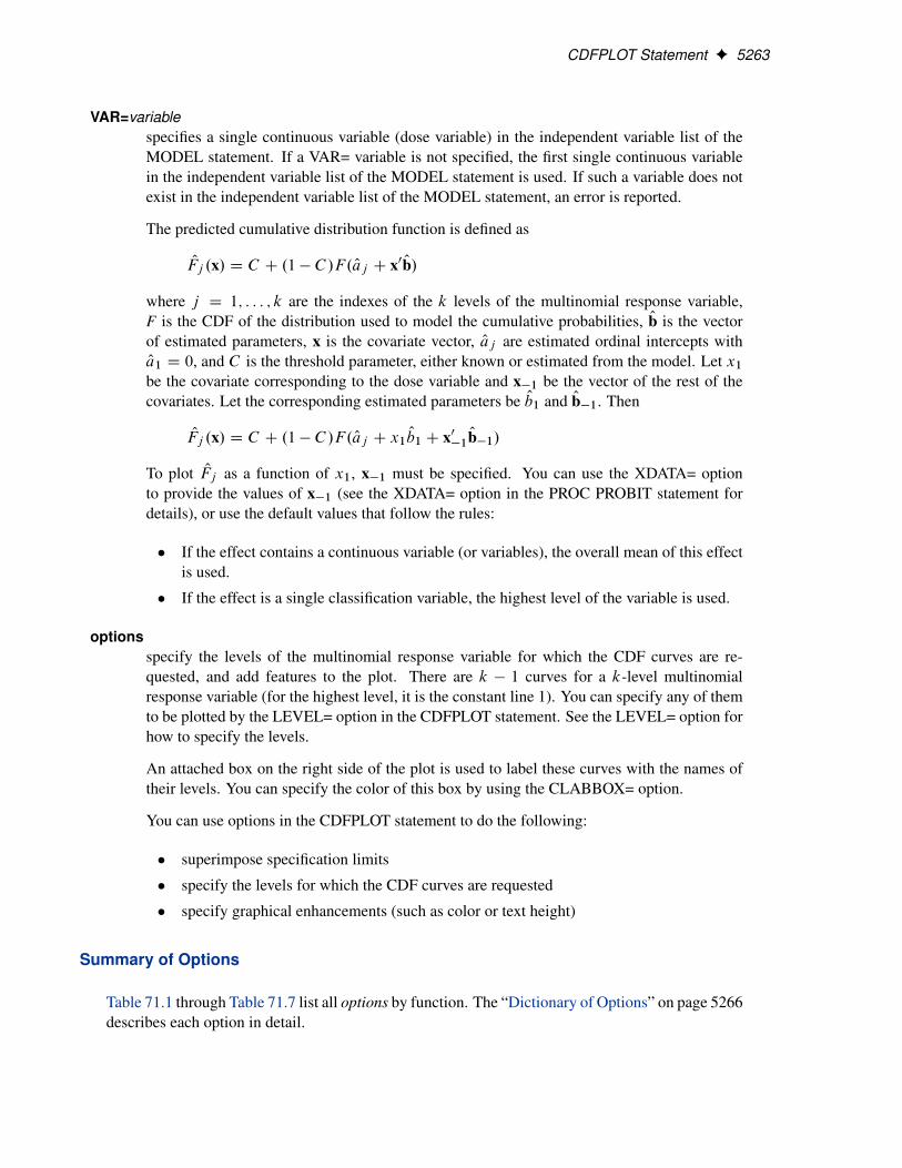
VAR=variablespecifies a single continuous variable (dose variable) in the independent variable list of theMODEL statement. If a VAR= variable is not specified, the first single continuous variablein the independent variable list of the MODEL statement is used. If such a variable does notexist in the independent variable list of the MODEL statement, an error is reported.
The predicted cumulative distribution function is defined as
OFj .x/ D C C .1 � C /F. Oaj C x0 Ob/
where j D 1; : : : ; k are the indexes of the k levels of the multinomial response variable,F is the CDF of the distribution used to model the cumulative probabilities, Ob is the vectorof estimated parameters, x is the covariate vector, Oaj are estimated ordinal intercepts withOa1 D 0, and C is the threshold parameter, either known or estimated from the model. Let x1
be the covariate corresponding to the dose variable and x�1 be the vector of the rest of thecovariates. Let the corresponding estimated parameters be Ob1 and Ob�1. Then
OFj .x/ D C C .1 � C /F. Oaj C x1Ob1 C x0
�1Ob�1/
To plot OFj as a function of x1, x�1 must be specified. You can use the XDATA= optionto provide the values of x�1 (see the XDATA= option in the PROC PROBIT statement fordetails), or use the default values that follow the rules:
� If the effect contains a continuous variable (or variables), the overall mean of this effectis used.
� If the effect is a single classification variable, the highest level of the variable is used.
optionsspecify the levels of the multinomial response variable for which the CDF curves are re-quested, and add features to the plot. There are k � 1 curves for a k-level multinomialresponse variable (for the highest level, it is the constant line 1). You can specify any of themto be plotted by the LEVEL= option in the CDFPLOT statement. See the LEVEL= option forhow to specify the levels.
An attached box on the right side of the plot is used to label these curves with the names oftheir levels. You can specify the color of this box by using the CLABBOX= option.
You can use options in the CDFPLOT statement to do the following:
� superimpose specification limits
� specify the levels for which the CDF curves are requested
� specify graphical enhancements (such as color or text height)
Summary of Options
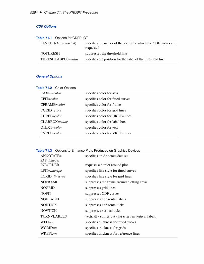
Table 71.1 through Table 71.7 list all options by function. The “Dictionary of Options” on page 5266describes each option in detail.
5264 F Chapter 71: The PROBIT Procedure
CDF Options
Table 71.1 Options for CDFPLOT
LEVEL=(character-list) specifies the names of the levels for which the CDF curves arerequested
NOTHRESH suppresses the threshold line
THRESHLABPOS=value specifies the position for the label of the threshold line
General Options
Table 71.2 Color Options
CAXIS=color specifies color for axis
CFIT=color specifies color for fitted curves
CFRAME=color specifies color for frame
CGRID=color specifies color for grid lines
CHREF=color specifies color for HREF= lines
CLABBOX=color specifies color for label box
CTEXT=color specifies color for text
CVREF=color specifies color for VREF= lines
Table 71.3 Options to Enhance Plots Produced on Graphics Devices
ANNOTATE=SAS-data-set
specifies an Annotate data set
INBORDER requests a border around plot
LFIT=linetype specifies line style for fitted curves
LGRID=linetype specifies line style for grid lines
NOFRAME suppresses the frame around plotting areas
NOGRID suppresses grid lines
NOFIT suppresses CDF curves
NOHLABEL suppresses horizontal labels
NOHTICK suppresses horizontal ticks
NOVTICK suppresses vertical ticks
TURNVLABELS vertically strings out characters in vertical labels
WFIT=n specifies thickness for fitted curves
WGRID=n specifies thickness for grids
WREFL=n specifies thickness for reference lines
CDFPLOT Statement F 5265
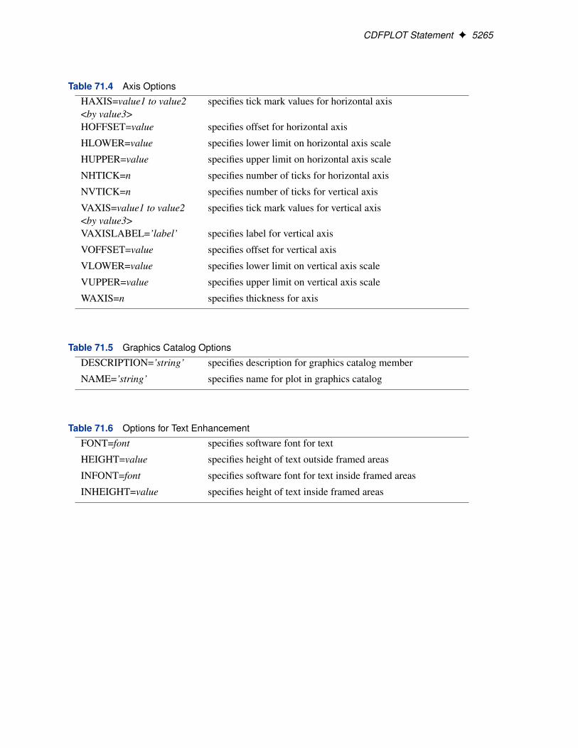
Table 71.4 Axis Options
HAXIS=value1 to value2<by value3>
specifies tick mark values for horizontal axis
HOFFSET=value specifies offset for horizontal axis
HLOWER=value specifies lower limit on horizontal axis scale
HUPPER=value specifies upper limit on horizontal axis scale
NHTICK=n specifies number of ticks for horizontal axis
NVTICK=n specifies number of ticks for vertical axis
VAXIS=value1 to value2<by value3>
specifies tick mark values for vertical axis
VAXISLABEL=’label’ specifies label for vertical axis
VOFFSET=value specifies offset for vertical axis
VLOWER=value specifies lower limit on vertical axis scale
VUPPER=value specifies upper limit on vertical axis scale
WAXIS=n specifies thickness for axis
Table 71.5 Graphics Catalog Options
DESCRIPTION=’string’ specifies description for graphics catalog member
NAME=’string’ specifies name for plot in graphics catalog
Table 71.6 Options for Text Enhancement
FONT=font specifies software font for text
HEIGHT=value specifies height of text outside framed areas
INFONT=font specifies software font for text inside framed areas
INHEIGHT=value specifies height of text inside framed areas
5266 F Chapter 71: The PROBIT Procedure
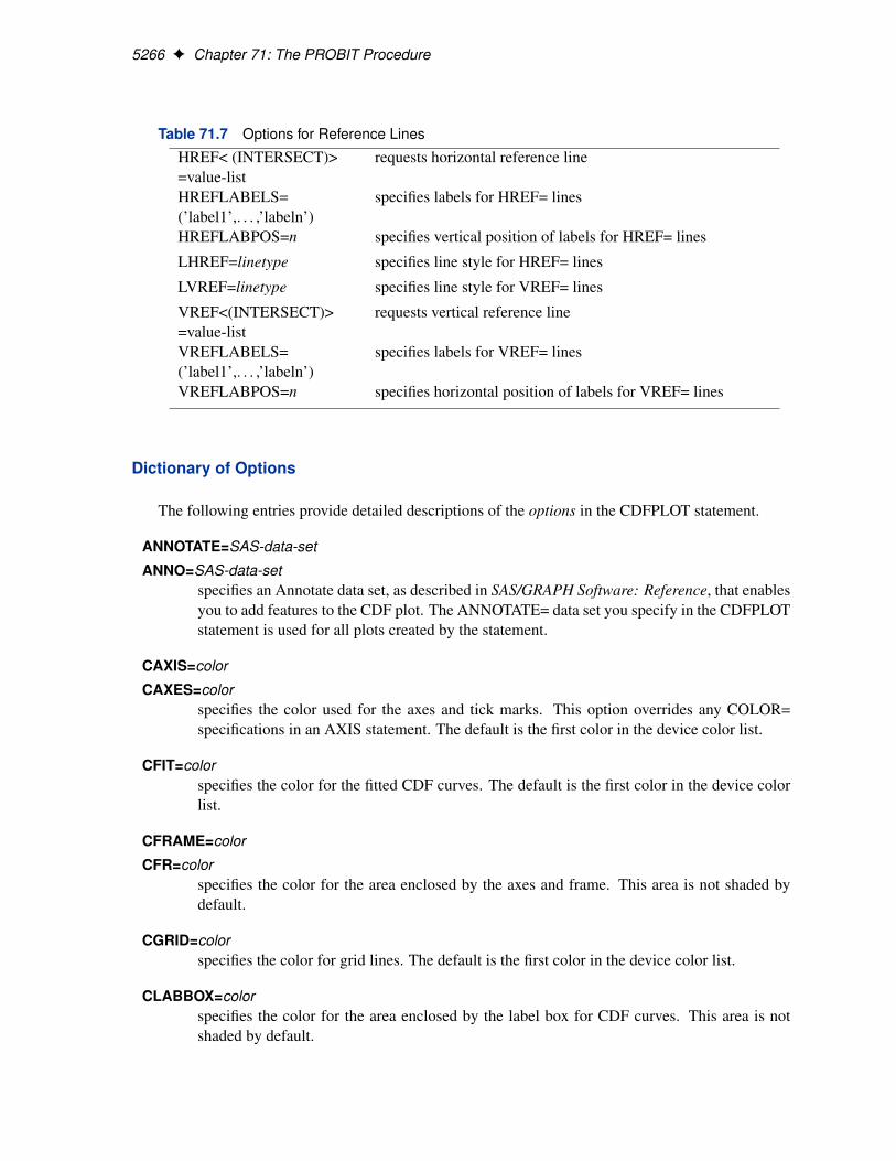
Table 71.7 Options for Reference Lines
HREF< (INTERSECT)>=value-list
requests horizontal reference line
HREFLABELS=(’label1’,. . . ,’labeln’)
specifies labels for HREF= lines
HREFLABPOS=n specifies vertical position of labels for HREF= lines
LHREF=linetype specifies line style for HREF= lines
LVREF=linetype specifies line style for VREF= lines
VREF<(INTERSECT)>=value-list
requests vertical reference line
VREFLABELS=(’label1’,. . . ,’labeln’)
specifies labels for VREF= lines
VREFLABPOS=n specifies horizontal position of labels for VREF= lines
Dictionary of Options
The following entries provide detailed descriptions of the options in the CDFPLOT statement.
ANNOTATE=SAS-data-set
ANNO=SAS-data-setspecifies an Annotate data set, as described in SAS/GRAPH Software: Reference, that enablesyou to add features to the CDF plot. The ANNOTATE= data set you specify in the CDFPLOTstatement is used for all plots created by the statement.
CAXIS=color
CAXES=colorspecifies the color used for the axes and tick marks. This option overrides any COLOR=specifications in an AXIS statement. The default is the first color in the device color list.
CFIT=colorspecifies the color for the fitted CDF curves. The default is the first color in the device colorlist.
CFRAME=color
CFR=colorspecifies the color for the area enclosed by the axes and frame. This area is not shaded bydefault.
CGRID=colorspecifies the color for grid lines. The default is the first color in the device color list.
CLABBOX=colorspecifies the color for the area enclosed by the label box for CDF curves. This area is notshaded by default.
CDFPLOT Statement F 5267
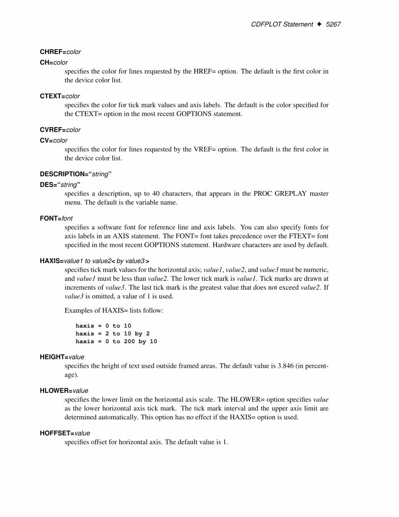
CHREF=color
CH=colorspecifies the color for lines requested by the HREF= option. The default is the first color inthe device color list.
CTEXT=colorspecifies the color for tick mark values and axis labels. The default is the color specified forthe CTEXT= option in the most recent GOPTIONS statement.
CVREF=color
CV=colorspecifies the color for lines requested by the VREF= option. The default is the first color inthe device color list.
DESCRIPTION=“string”
DES=“string”specifies a description, up to 40 characters, that appears in the PROC GREPLAY mastermenu. The default is the variable name.
FONT=fontspecifies a software font for reference line and axis labels. You can also specify fonts foraxis labels in an AXIS statement. The FONT= font takes precedence over the FTEXT= fontspecified in the most recent GOPTIONS statement. Hardware characters are used by default.
HAXIS=value1 to value2< by value3 >specifies tick mark values for the horizontal axis; value1, value2, and value3 must be numeric,and value1 must be less than value2. The lower tick mark is value1. Tick marks are drawn atincrements of value3. The last tick mark is the greatest value that does not exceed value2. Ifvalue3 is omitted, a value of 1 is used.
Examples of HAXIS= lists follow:
haxis = 0 to 10haxis = 2 to 10 by 2haxis = 0 to 200 by 10
HEIGHT=valuespecifies the height of text used outside framed areas. The default value is 3.846 (in percent-age).
HLOWER=valuespecifies the lower limit on the horizontal axis scale. The HLOWER= option specifies valueas the lower horizontal axis tick mark. The tick mark interval and the upper axis limit aredetermined automatically. This option has no effect if the HAXIS= option is used.
HOFFSET=valuespecifies offset for horizontal axis. The default value is 1.
5268 F Chapter 71: The PROBIT Procedure
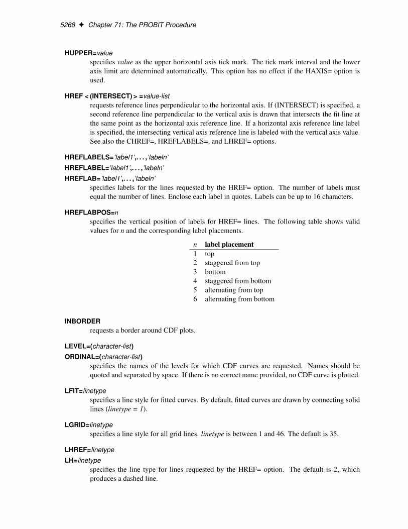
HUPPER=valuespecifies value as the upper horizontal axis tick mark. The tick mark interval and the loweraxis limit are determined automatically. This option has no effect if the HAXIS= option isused.
HREF < (INTERSECT) > =value-listrequests reference lines perpendicular to the horizontal axis. If (INTERSECT) is specified, asecond reference line perpendicular to the vertical axis is drawn that intersects the fit line atthe same point as the horizontal axis reference line. If a horizontal axis reference line labelis specified, the intersecting vertical axis reference line is labeled with the vertical axis value.See also the CHREF=, HREFLABELS=, and LHREF= options.
HREFLABELS=’label1’,. . . ,’labeln’
HREFLABEL=’label1’,. . . ,’labeln’
HREFLAB=’label1’,. . . ,’labeln’specifies labels for the lines requested by the HREF= option. The number of labels mustequal the number of lines. Enclose each label in quotes. Labels can be up to 16 characters.
HREFLABPOS=n
specifies the vertical position of labels for HREF= lines. The following table shows validvalues for n and the corresponding label placements.
n label placement1 top2 staggered from top3 bottom4 staggered from bottom5 alternating from top6 alternating from bottom
INBORDERrequests a border around CDF plots.
LEVEL=(character-list)
ORDINAL=(character-list)specifies the names of the levels for which CDF curves are requested. Names should bequoted and separated by space. If there is no correct name provided, no CDF curve is plotted.
LFIT=linetypespecifies a line style for fitted curves. By default, fitted curves are drawn by connecting solidlines (linetype = 1).
LGRID=linetypespecifies a line style for all grid lines. linetype is between 1 and 46. The default is 35.
LHREF=linetype
LH=linetypespecifies the line type for lines requested by the HREF= option. The default is 2, whichproduces a dashed line.
CDFPLOT Statement F 5269
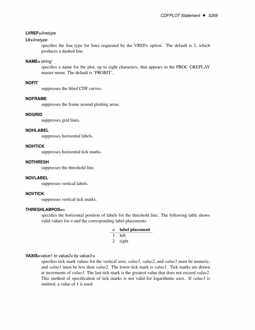
LVREF=linetype
LV=linetypespecifies the line type for lines requested by the VREF= option. The default is 2, whichproduces a dashed line.
NAME=’string’specifies a name for the plot, up to eight characters, that appears in the PROC GREPLAYmaster menu. The default is ’PROBIT’.
NOFITsuppresses the fitted CDF curves.
NOFRAMEsuppresses the frame around plotting areas.
NOGRIDsuppresses grid lines.
NOHLABELsuppresses horizontal labels.
NOHTICKsuppresses horizontal tick marks.
NOTHRESHsuppresses the threshold line.
NOVLABELsuppresses vertical labels.
NOVTICKsuppresses vertical tick marks.
THRESHLABPOS=n
specifies the horizontal position of labels for the threshold line. The following table showsvalid values for n and the corresponding label placements.
n label placement1 left2 right
VAXIS=value1 to value2< by value3 >specifies tick mark values for the vertical axis; value1, value2, and value3 must be numeric,and value1 must be less than value2. The lower tick mark is value1. Tick marks are drawnat increments of value3. The last tick mark is the greatest value that does not exceed value2.This method of specification of tick marks is not valid for logarithmic axes. If value3 isomitted, a value of 1 is used.

5270 F Chapter 71: The PROBIT Procedure
Examples of VAXIS= lists follow:
vaxis = 0 to 10vaxis = 0 to 2 by .1
VAXISLABEL=’string’specifies a label for the vertical axis.
VLOWER=valuespecifies the lower limit on the vertical axis scale. The VLOWER= option specifies valueas the lower vertical axis tick mark. The tick mark interval and the upper axis limit aredetermined automatically. This option has no effect if the VAXIS= option is used.
VREF=value-listrequests reference lines perpendicular to the vertical axis. If (INTERSECT) is specified, asecond reference line perpendicular to the horizontal axis is drawn that intersects the fit lineat the same point as the vertical axis reference line. If a vertical axis reference line label isspecified, the intersecting horizontal axis reference line is labeled with the horizontal axisvalue. See also the CVREF=, LVREF=, and VREFLABELS= options.
VREFLABELS=’label1’,. . . ,’labeln’
VREFLABEL=’label1’,. . . ,’labeln’
VREFLAB=’label1’,. . . ,’labeln’specifies labels for the lines requested by the VREF= option. The number of labels mustequal the number of lines. Enclose each label in quotes. Labels can be up to 16 characters.
VREFLABPOS=n
specifies the horizontal position of labels for VREF= lines. The following table shows validvalues for n and the corresponding label placements.
n label placement1 left2 right
VUPPER=valuespecifies the upper limit on the vertical axis scale. The VUPPER= option specifies value as theupper vertical axis tick mark. The tick mark interval and the lower axis limit are determinedautomatically. This option has no effect if the VAXIS= option is used.
WAXIS=n
specifies line thickness for axes and frame. The default value is 1.
WFIT=n
specifies line thickness for fitted curves. The default value is 1.
WGRID=n
specifies line thickness for grids. The default value is 1.
WREFL=n
specifies line thickness for reference lines. The default value is 1.
CLASS Statement F 5271
CLASS Statement
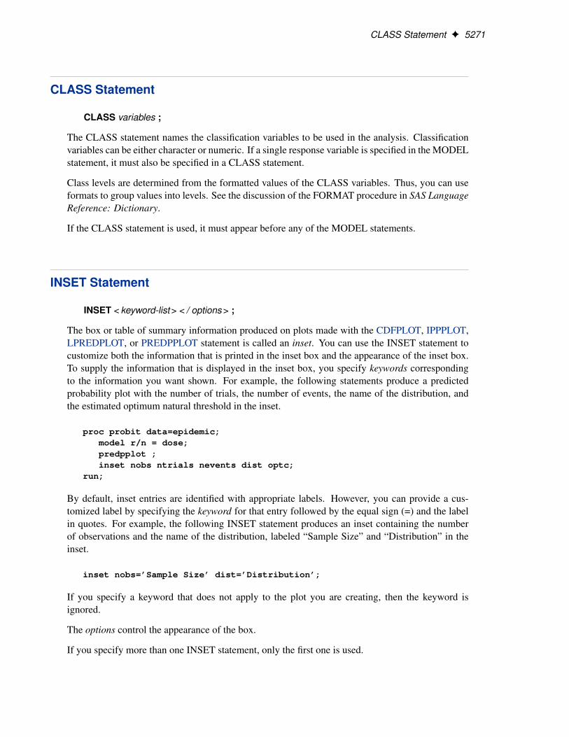
CLASS variables ;
The CLASS statement names the classification variables to be used in the analysis. Classificationvariables can be either character or numeric. If a single response variable is specified in the MODELstatement, it must also be specified in a CLASS statement.
Class levels are determined from the formatted values of the CLASS variables. Thus, you can useformats to group values into levels. See the discussion of the FORMAT procedure in SAS LanguageReference: Dictionary.
If the CLASS statement is used, it must appear before any of the MODEL statements.
INSET Statement
INSET < keyword-list > < / options > ;
The box or table of summary information produced on plots made with the CDFPLOT, IPPPLOT,LPREDPLOT, or PREDPPLOT statement is called an inset. You can use the INSET statement tocustomize both the information that is printed in the inset box and the appearance of the inset box.To supply the information that is displayed in the inset box, you specify keywords correspondingto the information you want shown. For example, the following statements produce a predictedprobability plot with the number of trials, the number of events, the name of the distribution, andthe estimated optimum natural threshold in the inset.
proc probit data=epidemic;model r/n = dose;predpplot ;inset nobs ntrials nevents dist optc;
run;
By default, inset entries are identified with appropriate labels. However, you can provide a cus-tomized label by specifying the keyword for that entry followed by the equal sign (=) and the labelin quotes. For example, the following INSET statement produces an inset containing the numberof observations and the name of the distribution, labeled “Sample Size” and “Distribution” in theinset.
inset nobs=’Sample Size’ dist=’Distribution’;
If you specify a keyword that does not apply to the plot you are creating, then the keyword isignored.
The options control the appearance of the box.
If you specify more than one INSET statement, only the first one is used.
5272 F Chapter 71: The PROBIT Procedure
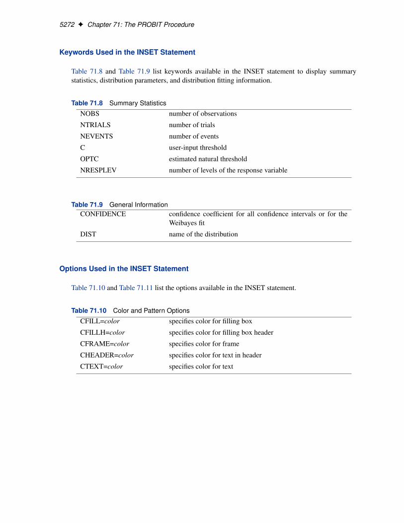
Keywords Used in the INSET Statement
Table 71.8 and Table 71.9 list keywords available in the INSET statement to display summarystatistics, distribution parameters, and distribution fitting information.
Table 71.8 Summary Statistics
NOBS number of observations
NTRIALS number of trials
NEVENTS number of events
C user-input threshold
OPTC estimated natural threshold
NRESPLEV number of levels of the response variable
Table 71.9 General InformationCONFIDENCE confidence coefficient for all confidence intervals or for the
Weibayes fit
DIST name of the distribution
Options Used in the INSET Statement
Table 71.10 and Table 71.11 list the options available in the INSET statement.
Table 71.10 Color and Pattern Options
CFILL=color specifies color for filling box
CFILLH=color specifies color for filling box header
CFRAME=color specifies color for frame
CHEADER=color specifies color for text in header
CTEXT=color specifies color for text
IPPPLOT Statement F 5273
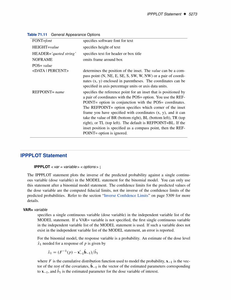
Table 71.11 General Appearance Options
FONT=font specifies software font for text
HEIGHT=value specifies height of text
HEADER=’quoted string’ specifies text for header or box titleNOFRAME omits frame around boxPOS= value<DATA | PERCENT> determines the position of the inset. The value can be a com-
pass point (N, NE, E, SE, S, SW, W, NW) or a pair of coordi-nates (x, y) enclosed in parentheses. The coordinates can bespecified in axis percentage units or axis data units.
REFPOINT= name specifies the reference point for an inset that is positioned bya pair of coordinates with the POS= option. You use the REF-POINT= option in conjunction with the POS= coordinates.The REFPOINT= option specifies which corner of the insetframe you have specified with coordinates (x, y), and it cantake the value of BR (bottom right), BL (bottom left), TR (topright), or TL (top left). The default is REFPOINT=BL. If theinset position is specified as a compass point, then the REF-POINT= option is ignored.
IPPPLOT Statement
IPPPLOT < var = variable > < options > ;
The IPPPLOT statement plots the inverse of the predicted probability against a single continu-ous variable (dose variable) in the MODEL statement for the binomial model. You can only usethis statement after a binomial model statement. The confidence limits for the predicted values ofthe dose variable are the computed fiducial limits, not the inverse of the confidence limits of thepredicted probabilities. Refer to the section “Inverse Confidence Limits” on page 5309 for moredetails.
VAR= variablespecifies a single continuous variable (dose variable) in the independent variable list of theMODEL statement. If a VAR= variable is not specified, the first single continuous variablein the independent variable list of the MODEL statement is used. If such a variable does notexist in the independent variable list of the MODEL statement, an error is reported.
For the binomial model, the response variable is a probability. An estimate of the dose levelOx1 needed for a response of p is given by
Ox1 D .F �1.p/ � x0�1
Ob�1/= Ob1
where F is the cumulative distribution function used to model the probability, x�1 is the vec-tor of the rest of the covariates, Ob�1 is the vector of the estimated parameters correspondingto x�1, and Ob1 is the estimated parameter for the dose variable of interest.
5274 F Chapter 71: The PROBIT Procedure
To plot Ox1 as a function of p, x�1 must be specified. You can use the XDATA= optionto provide the values of x�1 (see the XDATA= option in the PROC PROBIT statement fordetails), or use the default values that follow the rules:
� If the effect contains a continuous variable (or variables), the overall mean of this effectis used.
� If the effect is a single classification variable, the highest level of the variable is used.
optionsadd features to the plot.
You can use options in the IPPPLOT statement to do the following:
� superimpose specification limits
� suppress or add the observed data points on the plot
� suppress or add the fiducial limits on the plot
� specify graphical enhancements (such as color or text height)
Summary of Options
Table 71.12 through Table 71.18 list all options by function. The “Dictionary of Options” onpage 5276 describes each option in detail.
IPP Options
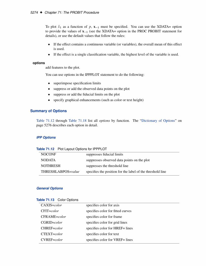
Table 71.12 Plot Layout Options for IPPPLOT
NOCONF suppresses fiducial limits
NODATA suppresses observed data points on the plot
NOTHRESH suppresses the threshold line
THRESHLABPOS=value specifies the position for the label of the threshold line
General Options
Table 71.13 Color Options
CAXIS=color specifies color for axis
CFIT=color specifies color for fitted curves
CFRAME=color specifies color for frame
CGRID=color specifies color for grid lines
CHREF=color specifies color for HREF= lines
CTEXT=color specifies color for text
CVREF=color specifies color for VREF= lines
IPPPLOT Statement F 5275
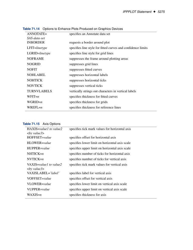
Table 71.14 Options to Enhance Plots Produced on Graphics Devices
ANNOTATE=SAS-data-set
specifies an Annotate data set
INBORDER requests a border around plot
LFIT=linetype specifies line style for fitted curves and confidence limits
LGRID=linetype specifies line style for grid lines
NOFRAME suppresses the frame around plotting areas
NOGRID suppresses grid lines
NOFIT suppresses fitted curves
NOHLABEL suppresses horizontal labels
NOHTICK suppresses horizontal ticks
NOVTICK suppresses vertical ticks
TURNVLABELS vertically strings out characters in vertical labels
WFIT=n specifies thickness for fitted curves
WGRID=n specifies thickness for grids
WREFL=n specifies thickness for reference lines
Table 71.15 Axis Options
HAXIS=value1 to value2<by value3>
specifies tick mark values for horizontal axis
HOFFSET=value specifies offset for horizontal axis
HLOWER=value specifies lower limit on horizontal axis scale
HUPPER=value specifies upper limit on horizontal axis scale
NHTICK=n specifies number of ticks for horizontal axis
NVTICK=n specifies number of ticks for vertical axis
VAXIS=value1 to value2<by value3>
specifies tick mark values for vertical axis
VAXISLABEL=’label’ specifies label for vertical axis
VOFFSET=value specifies offset for vertical axis
VLOWER=value specifies lower limit on vertical axis scale
VUPPER=value specifies upper limit on vertical axis scale
WAXIS=n specifies thickness for axis
5276 F Chapter 71: The PROBIT Procedure
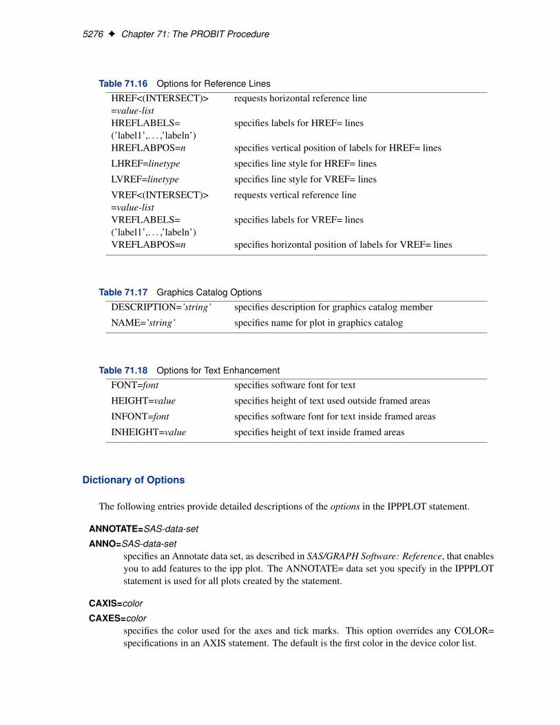
Table 71.16 Options for Reference Lines
HREF<(INTERSECT)>=value-list
requests horizontal reference line
HREFLABELS=(’label1’,. . . ,’labeln’)
specifies labels for HREF= lines
HREFLABPOS=n specifies vertical position of labels for HREF= lines
LHREF=linetype specifies line style for HREF= lines
LVREF=linetype specifies line style for VREF= lines
VREF<(INTERSECT)>=value-list
requests vertical reference line
VREFLABELS=(’label1’,. . . ,’labeln’)
specifies labels for VREF= lines
VREFLABPOS=n specifies horizontal position of labels for VREF= lines
Table 71.17 Graphics Catalog Options
DESCRIPTION=’string’ specifies description for graphics catalog member
NAME=’string’ specifies name for plot in graphics catalog
Table 71.18 Options for Text Enhancement
FONT=font specifies software font for text
HEIGHT=value specifies height of text used outside framed areas
INFONT=font specifies software font for text inside framed areas
INHEIGHT=value specifies height of text inside framed areas
Dictionary of Options
The following entries provide detailed descriptions of the options in the IPPPLOT statement.
ANNOTATE=SAS-data-set
ANNO=SAS-data-setspecifies an Annotate data set, as described in SAS/GRAPH Software: Reference, that enablesyou to add features to the ipp plot. The ANNOTATE= data set you specify in the IPPPLOTstatement is used for all plots created by the statement.
CAXIS=color
CAXES=colorspecifies the color used for the axes and tick marks. This option overrides any COLOR=specifications in an AXIS statement. The default is the first color in the device color list.
IPPPLOT Statement F 5277
CFIT=colorspecifies the color for the fitted ipp curves. The default is the first color in the device colorlist.
CFRAME=color
CFR=colorspecifies the color for the area enclosed by the axes and frame. This area is not shaded bydefault.
CGRID=colorspecifies the color for grid lines. The default is the first color in the device color list.
CHREF=color
CH=colorspecifies the color for lines requested by the HREF= option. The default is the first color inthe device color list.
CTEXT=colorspecifies the color for tick mark values and axis labels. The default is the color specified forthe CTEXT= option in the most recent GOPTIONS statement.
CVREF=color
CV=colorspecifies the color for lines requested by the VREF= option. The default is the first color inthe device color list.
DESCRIPTION=’string’
DES=’string’specifies a description, up to 40 characters, that appears in the PROC GREPLAY mastermenu. The default is the variable name.
FONT=fontspecifies a software font for reference line and axis labels. You can also specify fonts foraxis labels in an AXIS statement. The FONT= font takes precedence over the FTEXT= fontspecified in the most recent GOPTIONS statement. Hardware characters are used by default.
HAXIS=value1 to value2< by value3 >specifies tick mark values for the horizontal axis; value1, value2, and value3 must be numeric,and value1 must be less than value2. The lower tick mark is value1. Tick marks are drawn atincrements of value3. The last tick mark is the greatest value that does not exceed value2. Ifvalue3 is omitted, a value of 1 is used.
Examples of HAXIS= lists follow:
haxis = 0 to 10haxis = 2 to 10 by 2haxis = 0 to 200 by 10
HEIGHT=valuespecifies the height of text used outside framed areas. The default value is 3.846 (in percent-age).
5278 F Chapter 71: The PROBIT Procedure
HLOWER=valuespecifies the lower limit on the horizontal axis scale. The HLOWER= option specifies valueas the lower horizontal axis tick mark. The tick mark interval and the upper axis limit aredetermined automatically. This option has no effect if the HAXIS= option is used.
HOFFSET=valuespecifies offset for horizontal axis. The default value is 1.
HUPPER=valuespecifies value as the upper horizontal axis tick mark. The tick mark interval and the loweraxis limit are determined automatically. This option has no effect if the HAXIS= option isused.
HREF < (INTERSECT) > =value-listrequests reference lines perpendicular to the horizontal axis. If (INTERSECT) is specified, asecond reference line perpendicular to the vertical axis is drawn that intersects the fit line atthe same point as the horizontal axis reference line. If a horizontal axis reference line labelis specified, the intersecting vertical axis reference line is labeled with the vertical axis value.See also the CHREF=, HREFLABELS=, and LHREF= options.
HREFLABELS=’label1’,. . . ,’labeln’
HREFLABEL=’label1’,. . . ,’labeln’
HREFLAB=’label1’,. . . ,’labeln’specifies labels for the lines requested by the HREF= option. The number of labels mustequal the number of lines. Enclose each label in quotes. Labels can be up to 16 characters.
HREFLABPOS=n
specifies the vertical position of labels for HREF= lines. The following table shows validvalues for n and the corresponding label placements.
n label placement1 top2 staggered from top3 bottom4 staggered from bottom5 alternating from top6 alternating from bottom
INBORDERrequests a border around ipp plots.
LFIT=linetypespecifies a line style for fitted curves and confidence limits. By default, fitted curves aredrawn by connecting solid lines (linetype = 1) and confidence limits are drawn by connectingdashed lines (linetype = 3).
LGRID=linetypespecifies a line style for all grid lines. The value for linetype must be between 1 and 46. Thedefault is 35.
IPPPLOT Statement F 5279
LHREF=linetype
LH=linetypespecifies the line type for lines requested by the HREF= option. The default is 2, whichproduces a dashed line.
LVREF=linetype
LV=linetypespecifies the line type for lines requested by the VREF= option. The default is 2, whichproduces a dashed line.
NAME=’string’specifies a name for the plot, up to eight characters, that appears in the PROC GREPLAYmaster menu. The default is ’PROBIT’.
NOCONFsuppresses fiducial limits from the plot.
NODATAsuppresses observed data points from the plot.
NOFITsuppresses the fitted ipp curves.
NOFRAMEsuppresses the frame around plotting areas.
NOGRIDsuppresses grid lines.
NOHLABELsuppresses horizontal labels.
NOHTICKsuppresses horizontal tick marks.
NOTHRESHsuppresses the threshold line.
NOVLABELsuppresses vertical labels.
NOVTICKsuppresses vertical tick marks.
THRESHLABPOS=n
specifies the vertical position of labels for the threshold line. The following table shows validvalues for n and the corresponding label placements.
n label placement1 top2 bottom
5280 F Chapter 71: The PROBIT Procedure
VAXIS=value1 to value2< by value3 >specifies tick mark values for the vertical axis; value1, value2, and value3 must be numeric,and value1 must be less than value2. The lower tick mark is value1. Tick marks are drawnat increments of value3. The last tick mark is the greatest value that does not exceed value2.This method of specification of tick marks is not valid for logarithmic axes. If value3 isomitted, a value of 1 is used.
Examples of VAXIS= lists follow:
vaxis = 0 to 10vaxis = 0 to 2 by .1
VAXISLABEL=’string’specifies a label for the vertical axis.
VLOWER=valuespecifies the lower limit on the vertical axis scale. The VLOWER= option specifies valueas the lower vertical axis tick mark. The tick mark interval and the upper axis limit aredetermined automatically. This option has no effect if the VAXIS= option is used.
VREF=value-listrequests reference lines perpendicular to the vertical axis. If (INTERSECT) is specified, asecond reference line perpendicular to the horizontal axis is drawn that intersects the fit lineat the same point as the vertical axis reference line. If a vertical axis reference line label isspecified, the intersecting horizontal axis reference line is labeled with the horizontal axisvalue. See also the CVREF=, LVREF=, and VREFLABELS= options.
VREFLABELS=’label1’,. . . ,’labeln’
VREFLABEL=’label1’,. . . ,’labeln’
VREFLAB=’label1’,. . . ,’labeln’specifies labels for the lines requested by the VREF= option. The number of labels mustequal the number of lines. Enclose each label in quotes. Labels can be up to 16 characters.
VREFLABPOS=n
specifies the horizontal position of labels for VREF= lines. The following table shows validvalues for n and the corresponding label placements.
n label placement1 left2 right
VUPPER=valuespecifies the upper limit on the vertical axis scale. The VUPPER= option specifies value as theupper vertical axis tick mark. The tick mark interval and the lower axis limit are determinedautomatically. This option has no effect if the VAXIS= option is used.
WAXIS=n
specifies line thickness for axes and frame. The default value is 1.
LPREDPLOT Statement F 5281
WFIT=n
specifies line thickness for fitted curves. The default value is 1.
WGRID=n
specifies line thickness for grids. The default value is 1.
WREFL=n
specifies line thickness for reference lines. The default value is 1.
LPREDPLOT Statement
LPREDPLOT < var = variable > < options > ;
The LPREDPLOT statement plots the linear predictor x0b against a single continuous variable (dosevariable) in the MODEL statement for either the binomial model or the multinomial model. Theconfidence limits for the predicted values are available only for the binomial model.
VAR= variablespecifies a single continuous variable (dose variable) in the independent variable list of theMODEL statement for which the linear predictor plot is plotted. If a VAR= variable is notspecified, the first single continuous variable in the independent variable list of the MODELstatement is used. If such a variable does not exist in the independent variable list of theMODEL statement, an error is reported.
Let x1 be the covariate of the dose variable, x�1 be the vector of the rest of the covariates,Ob�1 be the vector of estimated parameters corresponding to x�1, and Ob1 be the estimatedparameter for the dose variable of interest.
To plot Ox0b as a function of x1, x�1 must be specified. You can use the XDATA= optionto provide the values of x�1 (see the XDATA= option in the PROC PROBIT statement fordetails), or use the default values that follow these rules:
� If the effect contains a continuous variable (or variables), the overall mean of this effectis used.
� If the effect is a single classification variable, the highest level of the variable is used.
optionsadd features to the plot.
For the multinomial model, you can use the LEVEL= option to specify the levels for whichthe linear predictor lines are plotted. The lines are labeled by the names of their levels in themiddle.
You can use options in the LPREDPLOT statement to do the following:
� superimpose specification limits
� suppress or add the observed data points on the plot for the binomial model
� suppress or add the confidence limits for the binomial model
5282 F Chapter 71: The PROBIT Procedure
� specify the levels for which the linear predictor lines are requested for the multinomialmodel
� specify graphical enhancements (such as color or text height)
Summary of Options
Table 71.19 through Table 71.25 list all options by function. The “Dictionary of Options” onpage 5284 describes each option in detail.
LPRED Options
Table 71.19 Plot Layout Options for LPREDPLOT
LEVEL=(character-list) specifies the names of the levels for which the linear predictorlines are requested (only for the multinomial model )
NOCONF suppresses fiducial limits (only for the binomial model)
NODATA suppresses observed data points on the plot (only for the bino-mial model)
NOTHRESH suppresses the threshold line
THRESHLABPOS=value specifies the position for the label of the threshold line
General Options
Table 71.20 Color Options
CAXIS=color specifies color for axis
CFIT=color specifies color for fitted curves
CFRAME=color specifies color for frame
CGRID=color specifies color for grid lines
CHREF=color specifies color for HREF= lines
CTEXT=color specifies color for text
CVREF=color specifies color for VREF= lines
LPREDPLOT Statement F 5283
Table 71.21 Options to Enhance Plots Produced on Graphics Devices
ANNOTATE=SAS-data-set
specifies an Annotate data set
INBORDER requests a border around plot
LFIT=linetype specifies line style for fitted curves and confidence limits
LGRID=linetype specifies line style for grid lines
NOFRAME suppresses the frame around plotting areas
NOGRID suppresses grid lines
NOFIT suppresses fitted curves
NOHLABEL suppresses horizontal labels
NOHTICK suppresses horizontal ticks
NOVTICK suppresses vertical ticks
TURNVLABELS vertically strings out characters in vertical labels
WFIT=n specifies thickness for fitted curves
WGRID=n specifies thickness for grids
WREFL=n specifies thickness for reference lines
Table 71.22 Axis Options
HAXIS=value1 to value2<by value3>
specifies tick mark values for horizontal axis
HOFFSET=value specifies offset for horizontal axis
HLOWER=value specifies lower limit on horizontal axis scale
HUPPER=value specifies upper limit on horizontal axis scale
NHTICK=n specifies number of ticks for horizontal axis
NVTICK=n specifies number of ticks for vertical axis
VAXIS=value1 to value2<by value3>
specifies tick mark values for vertical axis
VAXISLABEL=’label’ specifies label for vertical axis
VOFFSET=value specifies offset for vertical axis
VLOWER=value specifies lower limit on vertical axis scale
VUPPER=value specifies upper limit on vertical axis scale
WAXIS=n specifies thickness for axis
Table 71.23 Graphics Catalog Options
DESCRIPTION=’string’ specifies description for graphics catalog member
NAME=’string’ specifies name for plot in graphics catalog
5284 F Chapter 71: The PROBIT Procedure
Table 71.24 Options for Text Enhancement
FONT=font specifies software font for text
HEIGHT=value specifies height of text used outside framed areas
INFONT=font specifies software font for text inside framed areas
INHEIGHT=value specifies height of text inside framed areas
Table 71.25 Options for Reference Lines
HREF<(INTERSECT)>=value-list
requests horizontal reference line
HREFLABELS=(’label1’,. . . ,’labeln’)
specifies labels for HREF= lines
HREFLABPOS=n specifies vertical position of labels for HREF= lines
LHREF=linetype specifies line style for HREF= lines
LVREF=linetype specifies line style for VREF= lines
VREF<(INTERSECT)>=value-list
requests vertical reference line
VREFLABELS=(’label1’,. . . ,’labeln’)
specifies labels for VREF= lines
VREFLABPOS=n specifies horizontal position of labels for VREF= lines
Dictionary of Options
The following entries provide detailed descriptions of the options in the LPREDPLOT statement.
ANNOTATE=SAS-data-set
ANNO=SAS-data-setspecifies an Annotate data set, as described in SAS/GRAPH Software: Reference, that en-ables you to add features to the lpred plot. The ANNOTATE= data set you specify in theLPREDPLOT statement is used for all plots created by the statement.
CAXIS=color
CAXES=colorspecifies the color used for the axes and tick marks. This option overrides any COLOR=specifications in an AXIS statement. The default is the first color in the device color list.
CFIT=colorspecifies the color for the fitted lpred lines. The default is the first color in the device colorlist.
LPREDPLOT Statement F 5285
CFRAME=color
CFR=colorspecifies the color for the area enclosed by the axes and frame. This area is not shaded bydefault.
CGRID=colorspecifies the color for grid lines. The default is the first color in the device color list.
CHREF=color
CH=colorspecifies the color for lines requested by the HREF= option. The default is the first color inthe device color list.
CTEXT=colorspecifies the color for tick mark values and axis labels. The default is the color specified forthe CTEXT= option in the most recent GOPTIONS statement.
CVREF=color
CV=colorspecifies the color for lines requested by the VREF= option. The default is the first color inthe device color list.
DESCRIPTION=’string’
DES=’string’specifies a description, up to 40 characters, that appears in the PROC GREPLAY mastermenu. The default is the variable name.
FONT=fontspecifies a software font for reference line and axis labels. You can also specify fonts foraxis labels in an AXIS statement. The FONT= font takes precedence over the FTEXT= fontspecified in the most recent GOPTIONS statement. Hardware characters are used by default.
HAXIS=value1 to value2< by value3 >specifies tick mark values for the horizontal axis; value1, value2, and value3 must be numeric,and value1 must be less than value2. The lower tick mark is value1. Tick marks are drawn atincrements of value3. The last tick mark is the greatest value that does not exceed value2. Ifvalue3 is omitted, a value of 1 is used.
Examples of HAXIS= lists follow:
haxis = 0 to 10haxis = 2 to 10 by 2haxis = 0 to 200 by 10
HEIGHT=valuespecifies the height of text used outside framed areas. The default value is 3.846 (in percent-age).
5286 F Chapter 71: The PROBIT Procedure
HLOWER=valuespecifies the lower limit on the horizontal axis scale. The HLOWER= option specifies valueas the lower horizontal axis tick mark. The tick mark interval and the upper axis limit aredetermined automatically. This option has no effect if the HAXIS= option is used.
HOFFSET=valuespecifies offset for horizontal axis. The default value is 1.
HUPPER=valuespecifies value as the upper horizontal axis tick mark. The tick mark interval and the loweraxis limit are determined automatically. This option has no effect if the HAXIS= option isused.
HREF < (INTERSECT) > =value-listrequests reference lines perpendicular to the horizontal axis. If (INTERSECT) is specified, asecond reference line perpendicular to the vertical axis is drawn that intersects the fit line atthe same point as the horizontal axis reference line. If a horizontal axis reference line labelis specified, the intersecting vertical axis reference line is labeled with the vertical axis value.See also the CHREF=, HREFLABELS=, and LHREF= options.
HREFLABELS=’label1’,. . . ,’labeln’
HREFLABEL=’label1’,. . . ,’labeln’
HREFLAB=’label1’,. . . ,’labeln’specifies labels for the lines requested by the HREF= option. The number of labels mustequal the number of lines. Enclose each label in quotes. Labels can be up to 16 characters.
HREFLABPOS=n
specifies the vertical position of labels for HREF= lines. The following table shows validvalues for n and the corresponding label placements.
n label placement1 top2 staggered from top3 bottom4 staggered from bottom5 alternating from top6 alternating from bottom
INBORDERrequests a border around lpred plots.
LEVEL=(character-list)
ORDINAL=(character-list)specifies the names of the levels for which linear predictor lines are requested. Names shouldbe quoted and separated by space. If there is no correct name provided, no lpred line isplotted.
LPREDPLOT Statement F 5287
LFIT=linetypespecifies a line style for fitted curves and confidence limits. By default, fitted curves aredrawn by connecting solid lines (linetype = 1) and confidence limits are drawn by connectingdashed lines (linetype = 3).
LGRID=linetypespecifies a line style for all grid lines. The value for linetype is between 1 and 46. The defaultis 35.
LHREF=linetype
LH=linetypespecifies the line type for lines requested by the HREF= option. The default is 2, whichproduces a dashed line.
LVREF=linetype
LV=linetypespecifies the line type for lines requested by the VREF= option. The default is 2, whichproduces a dashed line.
NAME=’string’specifies a name for the plot, up to eight characters, that appears in the PROC GREPLAYmaster menu. The default is ’PROBIT’.
NOCONFsuppresses confidence limits from the plot. This works only for the binomial model. Confi-dence limits are not plotted for the multinomial model.
NODATAsuppresses observed data points from the plot. This works only for the binomial model. Datapoints are not plotted for the multinomial model.
NOFITsuppresses the fitted lpred lines.
NOFRAMEsuppresses the frame around plotting areas.
NOGRIDsuppresses grid lines.
NOHLABELsuppresses horizontal labels.
NOHTICKsuppresses horizontal tick marks.
NOTHRESHsuppresses the threshold line.
NOVLABELsuppresses vertical labels.
5288 F Chapter 71: The PROBIT Procedure
NOVTICKsuppresses vertical tick marks.
THRESHLABPOS=n
specifies the horizontal position of labels for the threshold line. The following table showsvalid values for n and the corresponding label placements.
n label placement1 left2 right
VAXIS=value1 to value2< by value3 >specifies tick mark values for the vertical axis; value1, value2, and value3 must be numeric,and value1 must be less than value2. The lower tick mark is value1. Tick marks are drawnat increments of value3. The last tick mark is the greatest value that does not exceed value2.This method of specification of tick marks is not valid for logarithmic axes. If value3 isomitted, a value of 1 is used.
Examples of VAXIS= lists follow:
vaxis = 0 to 10vaxis = 0 to 2 by .1
VAXISLABEL=’string’specifies a label for the vertical axis.
VLOWER=valuespecifies the lower limit on the vertical axis scale. The VLOWER= option specifies valueas the lower vertical axis tick mark. The tick mark interval and the upper axis limit aredetermined automatically. This option has no effect if the VAXIS= option is used.
VREF=value-listrequests reference lines perpendicular to the vertical axis. If (INTERSECT) is specified, asecond reference line perpendicular to the horizontal axis is drawn that intersects the fit lineat the same point as the vertical axis reference line. If a vertical axis reference line label isspecified, the intersecting horizontal axis reference line is labeled with the horizontal axisvalue. See also the CVREF=, LVREF=, and VREFLABELS= options.
VREFLABELS=’label1’,. . . ,’labeln’
VREFLABEL=’label1’,. . . ,’labeln’
VREFLAB=’label1’,. . . ,’labeln’specifies labels for the lines requested by the VREF= option. The number of labels mustequal the number of lines. Enclose each label in quotes. Labels can be up to 16 characters.
VREFLABPOS=n
specifies the horizontal position of labels for VREF= lines. The following table shows validvalues for n and the corresponding label placements.
n label placement1 left2 right
MODEL Statement F 5289
VUPPER=numberspecifies the upper limit on the vertical axis scale. The VUPPER= option specifies numberas the upper vertical axis tick mark. The tick mark interval and the lower axis limit aredetermined automatically. This option has no effect if the VAXIS= option is used.
WAXIS=n
specifies line thickness for axes and frame. The default value is 1.
WFIT=n
specifies line thickness for fitted lines. The default value is 1.
WGRID=n
specifies line thickness for grids. The default value is 1.
WREFL=n
specifies line thickness for reference lines. The default value is 1.
MODEL Statement
< label: > MODEL response=effects < / options > ;
< label: > MODEL events/trials=effects < / options > ;
The MODEL statement names the variables used as the response and the independent variables.Additionally, you can specify the distribution used to model the response, as well as other options.Only a single MODEL statement can be used with one invocation of the PROBIT procedure. Ifmultiple MODEL statements are present, only the last is used. Main effects and interaction termscan be specified in the MODEL statement, as in the GLM procedure.
The optional label, which must be a valid SAS name, is used to label output from the matchingMODEL statement.
The response can be a single variable with a value that is used to indicate the level of the observedresponse. For example, the response might be a variable called Symptoms that takes on the val-ues ‘None,’ ‘Mild,’ or ‘Severe.’ Note that, for dichotomous response variables, the probability ofthe lower sorted value is modeled by default (see the section “Details: PROBIT Procedure” onpage 5303). Because the model fit by the PROBIT procedure requires ordered response levels, youmight need to use either the ORDER=DATA option in the PROC PROBIT statement or a numericcoding of the response to get the desired ordering of levels.
Alternatively, the response can be specified as a pair of variable names separated by a slash (/). Thevalue of the first variable, events, is the number of positive responses (or events). The value of thesecond variable, trials, is the number of trials. Both variables must be numeric and nonnegative, andthe ratio of the first variable value to the second variable value must be between 0 and 1, inclusive.For example, the variables might be hits, a variable containing the number of hits for a baseballplayer, and AtBats, a variable containing the number of times at bat. A model for hitting proportion(batting average) as a function of age could be specified as
model hits/AtBats=age;
5290 F Chapter 71: The PROBIT Procedure
The effects following the equal sign are the covariates in the model. Higher-order effects, such asinteractions and nested terms, are allowed in the list, as in the GLM procedure. Variable names andcombinations of variable names representing higher-order terms are allowed to appear in this list.Classification variables can be used as effects, and indicator variables are generated for the classlevels. If you do not specify any covariates following the equal sign, an intercept-only model is fit.
The following options are available in the MODEL statement.
AGGREGATE
AGGREGATE=variable-listspecifies the subpopulations on which the Pearson chi-square test statistic and the log-likelihood ratio chi-square test statistic (deviance) are calculated if the LACKFIT option isspecified. See the section “Rescaling the Covariance Matrix” on page 5308 for details ofPearson’s chi-square and deviance calculations.
Observations with common values in the given list of variables are regarded as coming fromthe same subpopulation. Variables in the list can be any variables in the input data set. Spec-ifying the AGGREGATE option is equivalent to specifying the AGGREGATE= option witha variable list that includes all independent variables in the MODEL statement. The PROBITprocedure sorts the input data set according to the variables specified in this list. Informationfor the sorted data set is reported in the “Response-Covariate Profile” table.
The deviance and Pearson goodness-of-fit statistics are calculated if the LACKFIT option isspecified in the MODEL statement. The calculated results are reported in the “Goodness-of-Fit” table. If the Pearson chi-square test is significant with the test level specified by theHPROB= option, the fiducial limits, if required with the INVERSECL option in the MODELstatement, are modified (see the section “Inverse Confidence Limits” on page 5309 for de-tails). Also, the covariance matrix is rescaled by the dispersion parameter when the SCALE=option is specified.
ALPHA=valuesets the significance level for the confidence intervals for regression parameters, fiducial limitsfor the predicted values, and confidence intervals for the predicted probabilities. The valuemust be between 0 and 1. The default value is ALPHA=0.05.
CONVERGE=valuespecifies the convergence criterion. Convergence is declared when the maximum change inthe parameter estimates between Newton-Raphson steps is less than the value specified. Thechange is a relative change if the parameter is greater than 0.01 in absolute value; otherwise,it is an absolute change.
By default, CONVERGE=1.0E�8.
CORRBdisplays the estimated correlation matrix of the parameter estimates.
COVBdisplays the estimated covariance matrix of the parameter estimates.
MODEL Statement F 5291
DISTRIBUTION=distribution-type
DIST=distribution-type
D=distribution-typespecifies the cumulative distribution function used to model the response probabilities. Thedistributions are described in the section “Details: PROBIT Procedure” on page 5303. Validvalues for distribution-type are as follows:
NORMAL the normal distribution for the probit model
LOGISTIC the logistic distribution for the logit model
EXTREMEVALUE | EXTREME | GOMPERTZ the extreme value, or Gompertz distribu-tion for the gompit model
By default, DISTRIBUTION=NORMAL.
HPROB=pspecifies a minimum probability level for the Pearson chi-square to indicate a good fit. Thedefault value is 0.10. The LACKFIT option must also be specified for this option to haveany effect. For Pearson goodness-of-fit chi-square values with probability greater than theHPROB= value, the fiducial limits, if requested with the INVERSECL option, are computedby using a critical value of 1.96. For chi-square values with probability less than the valueof the HPROB= option, the critical value is a 0.95 two-sided quantile value taken from the t
distribution with degrees of freedom equal to .k �1/�m�q, where k is the number of levelsfor the response variable, m is the number of different sets of independent variable values,and q is the number of parameters fit in the model. If you specify the HPROB= option in boththe PROC PROBIT and MODEL statements, the MODEL statement option takes precedence.
INITIAL=valuessets initial values for the parameters in the model other than the intercept. The values must begiven in the order in which the variables are listed in the MODEL statement. If some of theindependent variables listed in the MODEL statement are classification variables, then theremust be as many values given for that variable as there are classification levels minus 1. TheINITIAL option can be specified as follows.
Type of List Specificationlist separated by blanks initial=3 4 5
list separated by commas initial=3,4,5
By default, all parameters have initial estimates of zero.
NOTE: The INITIAL= option is overwritten by the INEST= option in the PROC PROBITstatement.
INTERCEPT=valueinitializes the intercept parameter to value. By default, INTERCEPT=0.
INVERSECLcomputes confidence limits for the values of the first continuous independent variable (suchas dose) that yield selected response rates. If the algorithm fails to converge (this can happen
5292 F Chapter 71: The PROBIT Procedure
when C is nonzero), missing values are reported for the confidence limits. See the section“Inverse Confidence Limits” on page 5309 for details.
ITPRINTdisplays the iteration history, the final evaluation of the gradient, and the second derivativematrix (Hessian).
LACKFITperforms two goodness-of-fit tests (a Pearson chi-square test and a log-likelihood ratio chi-square test) for the fitted model.
To compute the test statistics, proper grouping of the observations into subpopulations isneeded. You can use the AGGREGATE or AGGREGATE= option for this purpose. See theentry for the AGGREGATE and AGGREGATE= options under the MODEL statement. Ifneither AGGREGATE nor AGGREGATE= is specified, PROC PROBIT assumes each obser-vation is from a separate subpopulation and computes the goodness-of-fit test statistics onlyfor the events/trials syntax.
NOTE: This test is not appropriate if the data are very sparse, with only a few values at eachset of the independent variable values.
If the Pearson chi-square test statistic is significant, then the covariance estimates and stan-dard error estimates are adjusted. See the section “Lack-of-Fit Tests” on page 5307 for adescription of the tests. Note that the LACKFIT option can also appear in the PROC PROBITstatement. See the section “PROC PROBIT Statement” on page 5258 for details.
MAXITER=value
MAXIT=valuespecifies the maximum number of iterations to be performed in estimating the parameters.By default, MAXITER=50.
NOINTfits a model with no intercept parameter. If the INTERCEPT= option is also specified, theintercept is fixed at the specified value; otherwise, it is set to zero. This is most useful whenthe response is binary. When the response has k levels, then k �1 intercept parameters are fit.The NOINT option sets the intercept parameter corresponding to the lowest response levelequal to zero. A Lagrange multiplier, or score, test for the restricted model is computed whenthe NOINT option is specified.
SCALE=scaleenables you to specify the method for estimating the dispersion parameter. To correct foroverdispersion or underdispersion, the covariance matrix is multiplied by the estimate of thedispersion parameter. Valid values for scale are as follows:
D | DEVIANCE specifies that the dispersion parameter be estimated by the deviancedivided by its degrees of freedom.
P | PEARSON specifies that the dispersion parameter be estimated by the Pearsonchi-square statistic divided by its degrees of freedom. This is set asthe default method for estimating the dispersion parameter.
OUTPUT Statement F 5293
You can use the AGGREGATE= option to define the subpopulations for calculating the Pear-son chi-square statistic and the deviance.
The “Goodness-of-Fit ” table includes the Pearson chi-square statistic, the deviance, theirdegrees of freedom, the ratio of each statistic divided by its degrees of freedom, and thecorresponding p-value.
SINGULAR=valuespecifies the singularity criterion for determining linear dependencies in the set of indepen-dent variables. The sum of squares and crossproducts matrix of the independent variables isformed and swept. If the relative size of a pivot becomes less than the value specified, thenthe variable corresponding to the pivot is considered to be linearly dependent on the previousset of variables considered. By default, SINGULAR=1E�12.
OUTPUT Statement
OUTPUT < OUT=SAS-data-set > keyword=name < . . . keyword=name > ;
The OUTPUT statement creates a new SAS data set containing all variables in the input data setand, optionally, the fitted probabilities, the estimate of x0ˇ, and the estimate of its standard error.Estimates of the probabilities, x0ˇ, and the standard errors are computed for observations withmissing response values as long as the values of all the explanatory variables are nonmissing. Thisenables you to compute these statistics for additional settings of the explanatory variables that areof interest but for which responses are not observed.
You can specify multiple OUTPUT statements. Each OUTPUT statement creates a new data setand applies only to the preceding MODEL statement. If you want to create a permanent SASdata set, you must specify a two-level name (refer to SAS Language Reference: Concepts for moreinformation about permanent SAS data sets).
Details on the specifications in the OUTPUT statement are as follows:
keyword=name specifies the statistics to include in the output data set and assigns namesto the new variables that contain the statistics. Specify a keyword for eachdesired statistic (see the following list of keywords), an equal sign, and thevariable to contain the statistic.
The keywords allowed and the statistics they represent are as follows:
PROB | P cumulative probability estimates
p D C C .1 � C /F.aj C x0ˇ/
STD standard error estimates of aj C x0b
XBETA estimates of aj C x0ˇ
OUT=SAS-data-set names the output data set. By default, the new data set is named by using theDATAn convention.
5294 F Chapter 71: The PROBIT Procedure
When the single variable response syntax is used, the _LEVEL_ variable is added to the output dataset, and there are k � 1 output observations for each input observation, where k is the numberof response levels. There is no observation output corresponding to the highest response level.For each of the k � 1 observations, the PROB variable contains the fitted probability of obtaininga response level up to the level indicated by the _LEVEL_ variable, the XBETA variable containsaj C x0b, where j references the levels (a1 D 0), and the STD variable contains the standard errorestimate of the XBETA variable. See the section “Details: PROBIT Procedure” on page 5303 for theformulas for the parameterizations.
PREDPPLOT Statement
PREDPPLOT < var = variable > < options > ;
The PREDPPLOT statement plots the predicted probability against a single continuous variable(dose variable) in the MODEL statement for both the binomial model and the multinomial model.Confidence limits are available only for the binomial model. An attached box on the right side of theplot is used to label predicted probability curves with the names of their levels for the multinomialmodel. You can specify the color of this box by using the CLABBOX= option.
VAR=variablespecifies a single continuous variable (dose variable) in the independent variable list of theMODEL statement. If a VAR= variable is not specified, the first single continuous variablein the independent variable list of the MODEL statement is used. If such a variable does notexist in the independent variable list of the MODEL statement, an error is reported.
The predicted probability is
Op D C C .1 � C /F.x0 Ob/
for the binomial model and
Op1 D C C .1 � C /F.x0 Ob/
Opj D .1 � C /.F. Oaj C x0 Ob/ � F. Oaj �1 C x0 Ob// j D 2; : : : ; k � 1
Opk D .1 � C /.1 � F. Oak�1 C x0 Ob//
for the multinomial model with k response levels, where F is the cumulative distributionfunction used to model the probability, x0 is the vector of the covariates, Oaj are the estimatedordinal intercepts with Oa1 D 0, C is the threshold parameter, either known or estimated fromthe model, and Ob0 is the vector of estimated parameters.
To plot Op (or Opj ) as a function of a continuous variable x1, the remaining covariates x�1 mustbe specified. You can use the XDATA= option to provide the values of x�1 (see the XDATA=option in the PROC PROBIT statement for details), or use the default values that follow theserules:
PREDPPLOT Statement F 5295
� If the effect contains a continuous variable (or variables), the overall mean of this effectis used.
� If the effect is a single classification variable, the highest level of the variable is used.
optionsenable you to plot the observed data and add features to the plot.
You can use options in the PREDPPLOT statement to do the following:
� superimpose specification limits
� suppress or add observed data points for the binomial model
� suppress or add confidence limits for the binomial model
� specify the levels for which predicted probability curves are requested for the multino-mial model
� specify graphical enhancements (such as color or text height)
Summary of Options
Table 71.26 through Table 71.32 list all options by function. The “Dictionary of Options” onpage 5298 describes each option in detail.
PREDPPLOT Options
Table 71.26 Plot Layout Options for PREDPPLOT
LEVEL=(character-list) specifies the names of the levels for which the predicted prob-ability curves are requested (only for the multinomial model)
NOCONF suppresses confidence limits
NODATA suppresses observed data points on the plot
NOTHRESH suppresses the threshold line
THRESHLABPOS=value specifies the position for the label of the threshold line
5296 F Chapter 71: The PROBIT Procedure
General Options
Table 71.27 Color Options
CAXIS=color specifies color for the axes
CFIT=color specifies color for fitted curves
CFRAME=color specifies color for frame
CGRID=color specifies color for grid lines
CHREF=color specifies color for HREF= lines
CLABBOX=color specifies color for label box
CTEXT=color specifies color for text
CVREF=color specifies color for VREF= lines
Table 71.28 Options to Enhance Plots Produced on Graphics Devices
ANNOTATE=SAS-data-set
specifies an Annotate data set
INBORDER requests a border around plot
LFIT=linetype specifies line style for fitted curves and confidence limits
LGRID=linetype specifies line style for grid lines
NOFRAME suppresses the frame around plotting areas
NOGRID suppresses grid lines
NOFIT suppresses fitted curves
NOHLABEL suppresses horizontal labels
NOHTICK suppresses horizontal ticks
NOVTICK suppresses vertical ticks
TURNVLABELS vertically strings out characters in vertical labels
WFIT=n specifies thickness for fitted curves
WGRID=n specifies thickness for grids
WREFL=n specifies thickness for reference lines
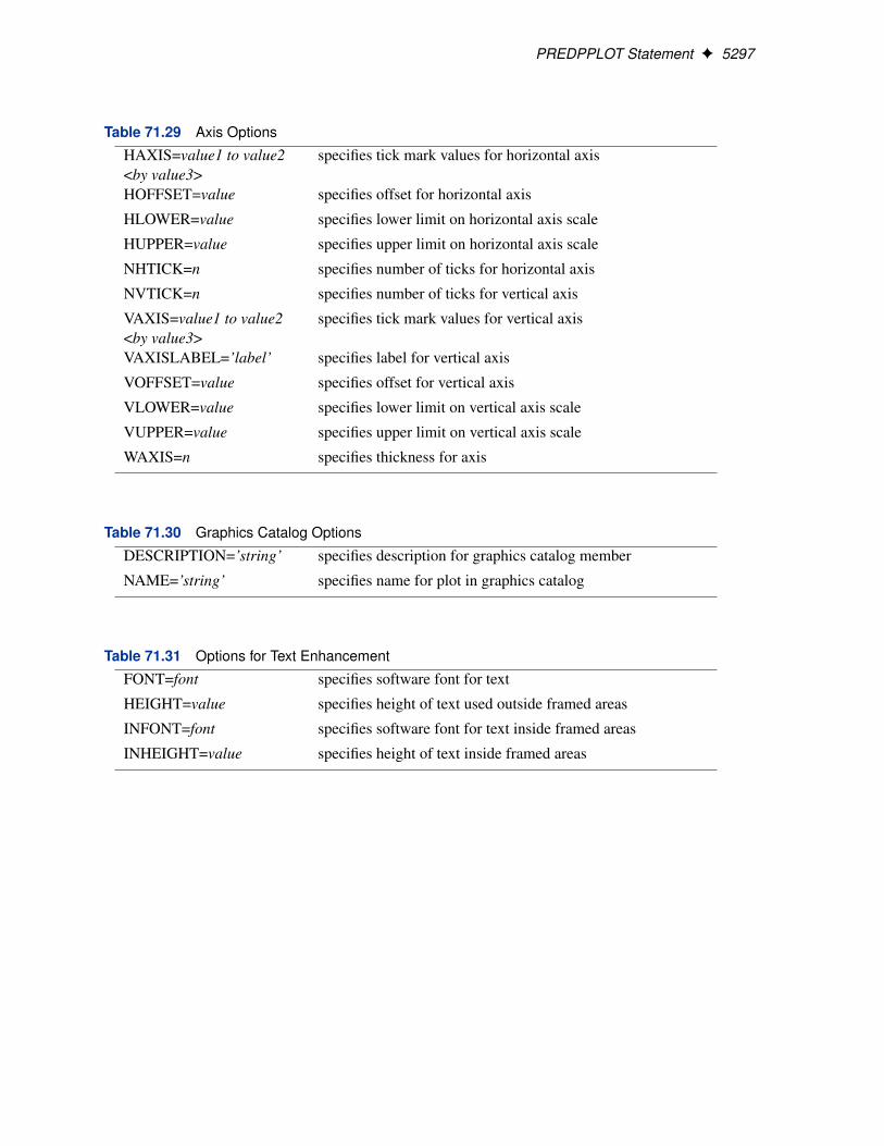
PREDPPLOT Statement F 5297
Table 71.29 Axis Options
HAXIS=value1 to value2<by value3>
specifies tick mark values for horizontal axis
HOFFSET=value specifies offset for horizontal axis
HLOWER=value specifies lower limit on horizontal axis scale
HUPPER=value specifies upper limit on horizontal axis scale
NHTICK=n specifies number of ticks for horizontal axis
NVTICK=n specifies number of ticks for vertical axis
VAXIS=value1 to value2<by value3>
specifies tick mark values for vertical axis
VAXISLABEL=’label’ specifies label for vertical axis
VOFFSET=value specifies offset for vertical axis
VLOWER=value specifies lower limit on vertical axis scale
VUPPER=value specifies upper limit on vertical axis scale
WAXIS=n specifies thickness for axis
Table 71.30 Graphics Catalog Options
DESCRIPTION=’string’ specifies description for graphics catalog member
NAME=’string’ specifies name for plot in graphics catalog
Table 71.31 Options for Text Enhancement
FONT=font specifies software font for text
HEIGHT=value specifies height of text used outside framed areas
INFONT=font specifies software font for text inside framed areas
INHEIGHT=value specifies height of text inside framed areas
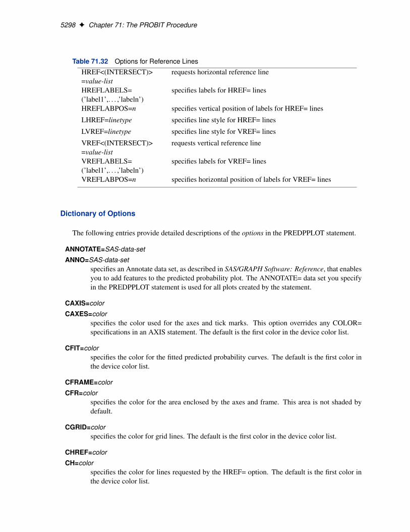
5298 F Chapter 71: The PROBIT Procedure
Table 71.32 Options for Reference Lines
HREF<(INTERSECT)>=value-list
requests horizontal reference line
HREFLABELS=(’label1’,. . . ,’labeln’)
specifies labels for HREF= lines
HREFLABPOS=n specifies vertical position of labels for HREF= lines
LHREF=linetype specifies line style for HREF= lines
LVREF=linetype specifies line style for VREF= lines
VREF<(INTERSECT)>=value-list
requests vertical reference line
VREFLABELS=(’label1’,. . . ,’labeln’)
specifies labels for VREF= lines
VREFLABPOS=n specifies horizontal position of labels for VREF= lines
Dictionary of Options
The following entries provide detailed descriptions of the options in the PREDPPLOT statement.
ANNOTATE=SAS-data-set
ANNO=SAS-data-setspecifies an Annotate data set, as described in SAS/GRAPH Software: Reference, that enablesyou to add features to the predicted probability plot. The ANNOTATE= data set you specifyin the PREDPPLOT statement is used for all plots created by the statement.
CAXIS=color
CAXES=colorspecifies the color used for the axes and tick marks. This option overrides any COLOR=specifications in an AXIS statement. The default is the first color in the device color list.
CFIT=colorspecifies the color for the fitted predicted probability curves. The default is the first color inthe device color list.
CFRAME=color
CFR=colorspecifies the color for the area enclosed by the axes and frame. This area is not shaded bydefault.
CGRID=colorspecifies the color for grid lines. The default is the first color in the device color list.
CHREF=color
CH=colorspecifies the color for lines requested by the HREF= option. The default is the first color inthe device color list.
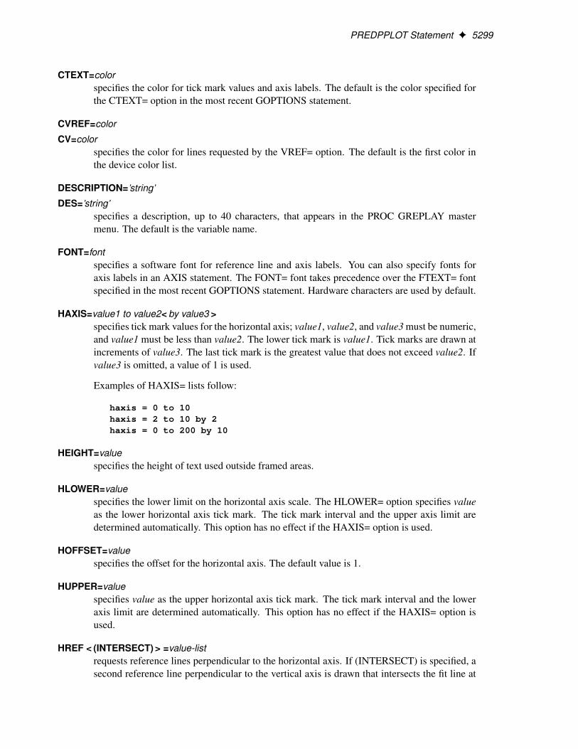
PREDPPLOT Statement F 5299
CTEXT=colorspecifies the color for tick mark values and axis labels. The default is the color specified forthe CTEXT= option in the most recent GOPTIONS statement.
CVREF=color
CV=colorspecifies the color for lines requested by the VREF= option. The default is the first color inthe device color list.
DESCRIPTION=’string’
DES=’string’specifies a description, up to 40 characters, that appears in the PROC GREPLAY mastermenu. The default is the variable name.
FONT=fontspecifies a software font for reference line and axis labels. You can also specify fonts foraxis labels in an AXIS statement. The FONT= font takes precedence over the FTEXT= fontspecified in the most recent GOPTIONS statement. Hardware characters are used by default.
HAXIS=value1 to value2< by value3 >specifies tick mark values for the horizontal axis; value1, value2, and value3 must be numeric,and value1 must be less than value2. The lower tick mark is value1. Tick marks are drawn atincrements of value3. The last tick mark is the greatest value that does not exceed value2. Ifvalue3 is omitted, a value of 1 is used.
Examples of HAXIS= lists follow:
haxis = 0 to 10haxis = 2 to 10 by 2haxis = 0 to 200 by 10
HEIGHT=valuespecifies the height of text used outside framed areas.
HLOWER=valuespecifies the lower limit on the horizontal axis scale. The HLOWER= option specifies valueas the lower horizontal axis tick mark. The tick mark interval and the upper axis limit aredetermined automatically. This option has no effect if the HAXIS= option is used.
HOFFSET=valuespecifies the offset for the horizontal axis. The default value is 1.
HUPPER=valuespecifies value as the upper horizontal axis tick mark. The tick mark interval and the loweraxis limit are determined automatically. This option has no effect if the HAXIS= option isused.
HREF < (INTERSECT) > =value-listrequests reference lines perpendicular to the horizontal axis. If (INTERSECT) is specified, asecond reference line perpendicular to the vertical axis is drawn that intersects the fit line at
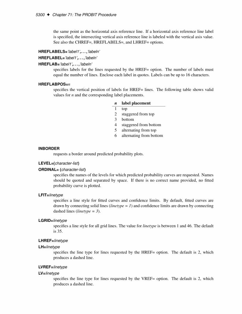
5300 F Chapter 71: The PROBIT Procedure
the same point as the horizontal axis reference line. If a horizontal axis reference line labelis specified, the intersecting vertical axis reference line is labeled with the vertical axis value.See also the CHREF=, HREFLABELS=, and LHREF= options.
HREFLABELS=’label1’,. . . ,’labeln’
HREFLABEL=’label1’,. . . ,’labeln’
HREFLAB=’label1’,. . . ,’labeln’specifies labels for the lines requested by the HREF= option. The number of labels mustequal the number of lines. Enclose each label in quotes. Labels can be up to 16 characters.
HREFLABPOS=n
specifies the vertical position of labels for HREF= lines. The following table shows validvalues for n and the corresponding label placements.
n label placement1 top2 staggered from top3 bottom4 staggered from bottom5 alternating from top6 alternating from bottom
INBORDERrequests a border around predicted probability plots.
LEVEL=(character-list)
ORDINAL= (character-list)specifies the names of the levels for which predicted probability curves are requested. Namesshould be quoted and separated by space. If there is no correct name provided, no fittedprobability curve is plotted.
LFIT=linetypespecifies a line style for fitted curves and confidence limits. By default, fitted curves aredrawn by connecting solid lines (linetype = 1) and confidence limits are drawn by connectingdashed lines (linetype = 3).
LGRID=linetypespecifies a line style for all grid lines. The value for linetype is between 1 and 46. The defaultis 35.
LHREF=linetype
LH=linetypespecifies the line type for lines requested by the HREF= option. The default is 2, whichproduces a dashed line.
LVREF=linetype
LV=linetypespecifies the line type for lines requested by the VREF= option. The default is 2, whichproduces a dashed line.
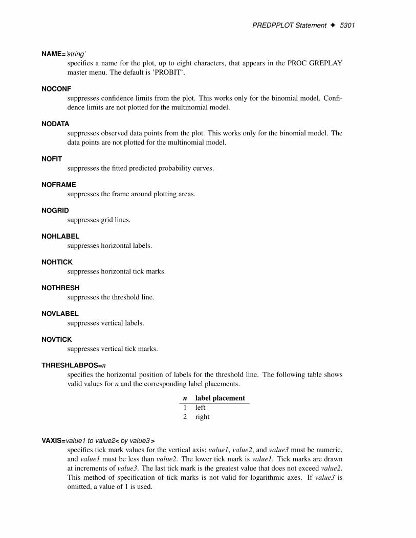
PREDPPLOT Statement F 5301
NAME=’string’specifies a name for the plot, up to eight characters, that appears in the PROC GREPLAYmaster menu. The default is ’PROBIT’.
NOCONFsuppresses confidence limits from the plot. This works only for the binomial model. Confi-dence limits are not plotted for the multinomial model.
NODATAsuppresses observed data points from the plot. This works only for the binomial model. Thedata points are not plotted for the multinomial model.
NOFITsuppresses the fitted predicted probability curves.
NOFRAMEsuppresses the frame around plotting areas.
NOGRIDsuppresses grid lines.
NOHLABELsuppresses horizontal labels.
NOHTICKsuppresses horizontal tick marks.
NOTHRESHsuppresses the threshold line.
NOVLABELsuppresses vertical labels.
NOVTICKsuppresses vertical tick marks.
THRESHLABPOS=n
specifies the horizontal position of labels for the threshold line. The following table showsvalid values for n and the corresponding label placements.
n label placement1 left2 right
VAXIS=value1 to value2< by value3 >specifies tick mark values for the vertical axis; value1, value2, and value3 must be numeric,and value1 must be less than value2. The lower tick mark is value1. Tick marks are drawnat increments of value3. The last tick mark is the greatest value that does not exceed value2.This method of specification of tick marks is not valid for logarithmic axes. If value3 isomitted, a value of 1 is used.
5302 F Chapter 71: The PROBIT Procedure
Examples of VAXIS= lists follow:
vaxis = 0 to 10vaxis = 0 to 2 by .1
VAXISLABEL=’string’specifies a label for the vertical axis.
VLOWER=valuespecifies the lower limit on the vertical axis scale. The VLOWER= option specifies valueas the lower vertical axis tick mark. The tick mark interval and the upper axis limit aredetermined automatically. This option has no effect if the VAXIS= option is used.
VREF=value-listrequests reference lines perpendicular to the vertical axis. If (INTERSECT) is specified, asecond reference line perpendicular to the horizontal axis is drawn that intersects the fit lineat the same point as the vertical axis reference line. If a vertical axis reference line label isspecified, the intersecting horizontal axis reference line is labeled with the horizontal axisvalue. See also the CVREF=, LVREF=, and VREFLABELS= options.
VREFLABELS=’label1’,. . . ,’labeln’
VREFLABEL=’label1’,. . . ,’labeln’
VREFLAB=’label1’,. . . ,’labeln’specifies labels for the lines requested by the VREF= option. The number of labels mustequal the number of lines. Enclose each label in quotes. Labels can be up to 16 characters.
VREFLABPOS=n
specifies the horizontal position of labels for VREF= lines. The following table shows validvalues for n and the corresponding label placements.
n label placement1 left2 right
VUPPER=valuespecifies the upper limit on the vertical axis scale. The VUPPER= option specifies value as theupper vertical axis tick mark. The tick mark interval and the lower axis limit are determinedautomatically. This option has no effect if the VAXIS= option is used.
WAXIS=n
specifies line thickness for axes and frame. The default value is 1.
WFIT=n
specifies line thickness for fitted curves. The default value is 1.
WGRID=n
specifies line thickness for grids. The default value is 1.
WREFL=n
specifies line thickness for reference lines. The default value is 1.
WEIGHT Statement F 5303
WEIGHT Statement
WEIGHT variable ;
A WEIGHT statement can be used with PROC PROBIT to weight each observation by the value ofthe variable specified. The contribution of each observation to the likelihood function is multipliedby the value of the weight variable. Observations with zero, negative, or missing weights are notused in model estimation.
Details: PROBIT Procedure
Missing Values
PROC PROBIT does not use any observations having missing values for any of the independentvariables, the response variables, or the weight variable. If only the response variables are missing,statistics requested in the OUTPUT statement are computed.
Response Level Ordering
For binary response data, PROC PROBIT fits the following model by default:
ˆ�1
�p � C
1 � C
�D x0ˇ
where p is the probability of the response level identified as the first level in the “Weighted Fre-quency Counts for the Ordered Response Categories” table in the output and ˆ is the normal cu-mulative distribution function. By default, the covariate vector x contains an intercept term. This issometimes called Abbot’s formula.
Because of the symmetry of the normal (and logistic) distribution, the effect of reversing the orderof the two response values is to change the signs of ˇ in the preceding equation.
By default, response levels appear in ascending, sorted order (that is, the lowest level appears first,and then the next lowest, and so on). There are a number of ways that you can control the sort orderof the response categories and, therefore, which level is assigned the first ordered level. One of themost common sets of response levels is {0,1}, with 1 representing the event with the probabilitythat is to be modeled.
Consider the example where Y takes the values 1 and 0 for event and nonevent, respectively, andEXPOSURE is the explanatory variable. By default, PROC PROBIT assigns the first ordered level
5304 F Chapter 71: The PROBIT Procedure
to response level 0, causing the probability of the nonevent to be modeled. There are several waysto change this.
Besides recoding the variable Y, you can do the following:
� assign a format to Y such that the first formatted value (when the formatted values are putin sorted order) corresponds to the event. For the following example, Y=0 could be assignedformatted value ‘nonevent’ and Y=1 could be assigned formatted value ‘event.’ Since OR-DER=FORMATTED by default, Y=1 becomes the first ordered level. See Example 71.3 foran illustration of this method.
proc format;value disease 1=’event’ 0=’nonevent’;
run;proc probit;
model y=exposure;format y disease.;
run;
� arrange the input data set so that Y=1 appears first and use the ORDER=DATA option in thePROC PROBIT statement. Since ORDER=DATA sorts levels in order of their appearance inthe data set, Y=1 becomes the first ordered level. Note that this option causes classificationvariables to be sorted by their order of appearance in the data set, also.
Computational Method
The log-likelihood function is maximized by means of a ridge-stabilized Newton-Raphson algo-rithm. Initial regression parameter estimates are set to zero. The INITIAL= and INTERCEPT=options in the MODEL statement can be used to give nonzero initial estimates.
The log-likelihood function, L, is computed as
L D
Xi
wi ln.pi /
where the sum is over the observations in the data set, wi is the weight for the i th observation, andpi is the modeled probability of the observed response. In the case of the events/trials syntax in theMODEL statement, each observation contributes two terms corresponding to the probability of theevent and the probability of its complement:
L D
Xi
wi Œri ln.pi / C .ni � ri / ln.1 � pi /�
where ri is the number of events and ni is the number of trials for observation i . This log-likelihoodfunction differs from the log-likelihood function for a binomial or multinomial distribution by addi-tive terms consisting of the log of binomial or multinomial coefficients. These terms are parameter-independent and do not affect the model estimation or the standard errors and tests.
The estimated covariance matrix, V, of the parameter estimates is computed as the negative inverseof the information matrix of second derivatives of L with respect to the parameters evaluated at
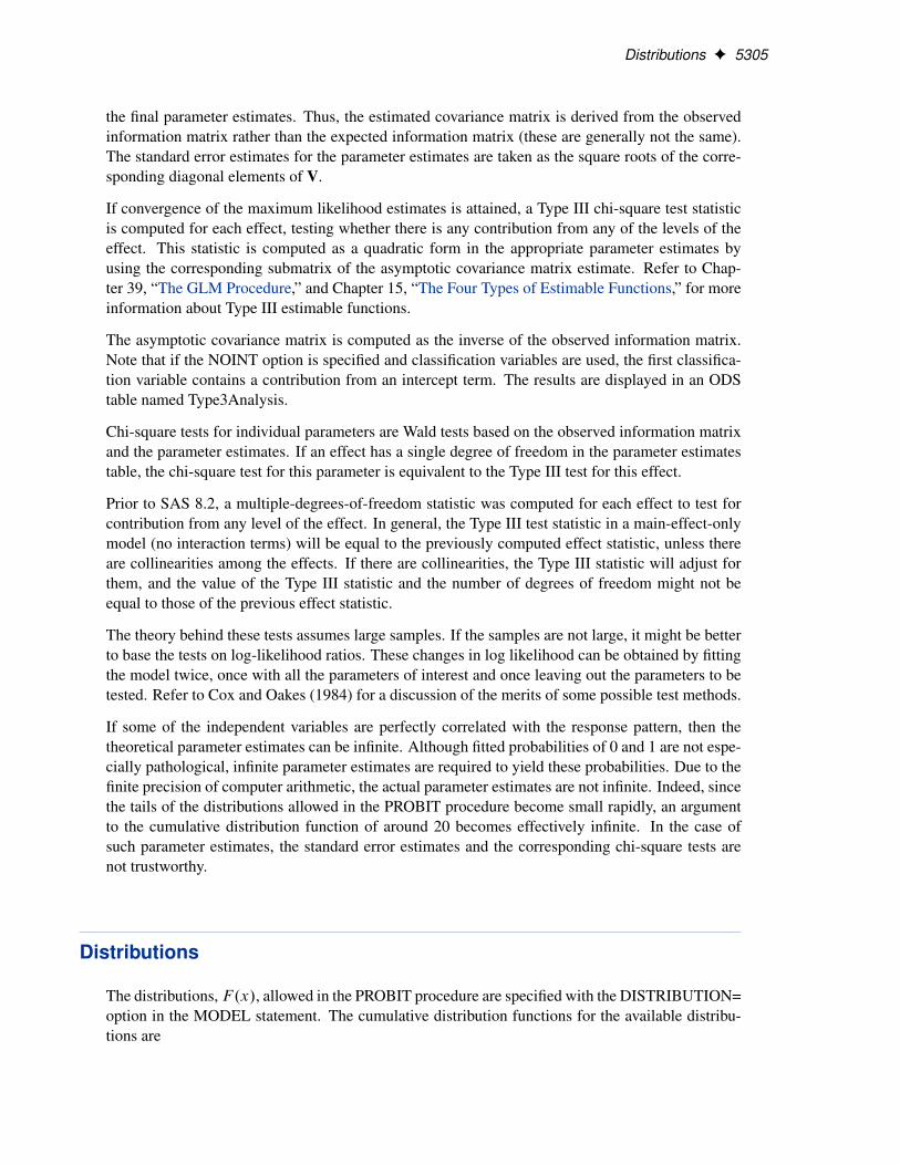
Distributions F 5305
the final parameter estimates. Thus, the estimated covariance matrix is derived from the observedinformation matrix rather than the expected information matrix (these are generally not the same).The standard error estimates for the parameter estimates are taken as the square roots of the corre-sponding diagonal elements of V.
If convergence of the maximum likelihood estimates is attained, a Type III chi-square test statisticis computed for each effect, testing whether there is any contribution from any of the levels of theeffect. This statistic is computed as a quadratic form in the appropriate parameter estimates byusing the corresponding submatrix of the asymptotic covariance matrix estimate. Refer to Chap-ter 39, “The GLM Procedure,” and Chapter 15, “The Four Types of Estimable Functions,” for moreinformation about Type III estimable functions.
The asymptotic covariance matrix is computed as the inverse of the observed information matrix.Note that if the NOINT option is specified and classification variables are used, the first classifica-tion variable contains a contribution from an intercept term. The results are displayed in an ODStable named Type3Analysis.
Chi-square tests for individual parameters are Wald tests based on the observed information matrixand the parameter estimates. If an effect has a single degree of freedom in the parameter estimatestable, the chi-square test for this parameter is equivalent to the Type III test for this effect.
Prior to SAS 8.2, a multiple-degrees-of-freedom statistic was computed for each effect to test forcontribution from any level of the effect. In general, the Type III test statistic in a main-effect-onlymodel (no interaction terms) will be equal to the previously computed effect statistic, unless thereare collinearities among the effects. If there are collinearities, the Type III statistic will adjust forthem, and the value of the Type III statistic and the number of degrees of freedom might not beequal to those of the previous effect statistic.
The theory behind these tests assumes large samples. If the samples are not large, it might be betterto base the tests on log-likelihood ratios. These changes in log likelihood can be obtained by fittingthe model twice, once with all the parameters of interest and once leaving out the parameters to betested. Refer to Cox and Oakes (1984) for a discussion of the merits of some possible test methods.
If some of the independent variables are perfectly correlated with the response pattern, then thetheoretical parameter estimates can be infinite. Although fitted probabilities of 0 and 1 are not espe-cially pathological, infinite parameter estimates are required to yield these probabilities. Due to thefinite precision of computer arithmetic, the actual parameter estimates are not infinite. Indeed, sincethe tails of the distributions allowed in the PROBIT procedure become small rapidly, an argumentto the cumulative distribution function of around 20 becomes effectively infinite. In the case ofsuch parameter estimates, the standard error estimates and the corresponding chi-square tests arenot trustworthy.
Distributions
The distributions, F.x/, allowed in the PROBIT procedure are specified with the DISTRIBUTION=option in the MODEL statement. The cumulative distribution functions for the available distribu-tions are
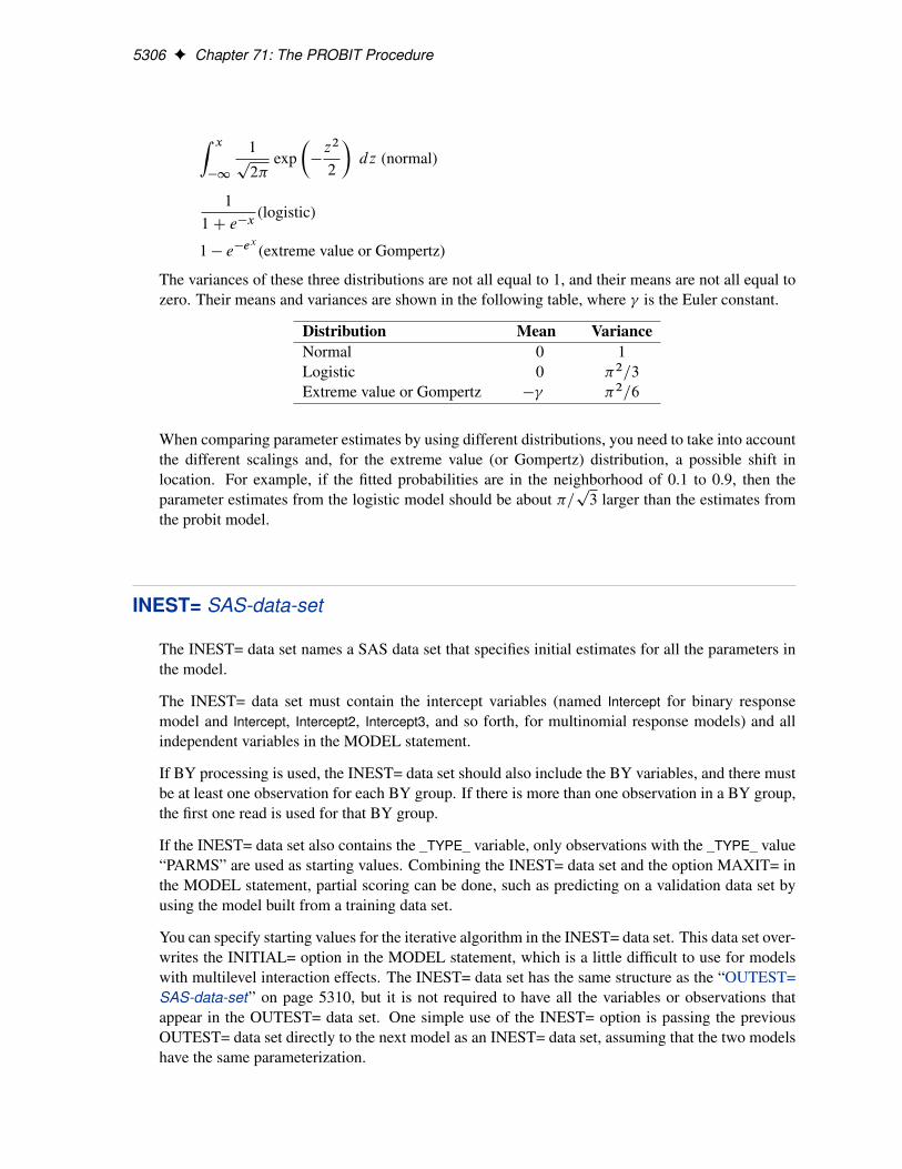
5306 F Chapter 71: The PROBIT Procedure
Z x
�1
1p
2�exp
��
z2
2
�dz (normal)
1
1 C e�x(logistic)
1 � e�ex
(extreme value or Gompertz)
The variances of these three distributions are not all equal to 1, and their means are not all equal tozero. Their means and variances are shown in the following table, where is the Euler constant.
Distribution Mean VarianceNormal 0 1Logistic 0 �2=3
Extreme value or Gompertz � �2=6
When comparing parameter estimates by using different distributions, you need to take into accountthe different scalings and, for the extreme value (or Gompertz) distribution, a possible shift inlocation. For example, if the fitted probabilities are in the neighborhood of 0.1 to 0.9, then theparameter estimates from the logistic model should be about �=
p3 larger than the estimates from
the probit model.
INEST= SAS-data-set
The INEST= data set names a SAS data set that specifies initial estimates for all the parameters inthe model.
The INEST= data set must contain the intercept variables (named Intercept for binary responsemodel and Intercept, Intercept2, Intercept3, and so forth, for multinomial response models) and allindependent variables in the MODEL statement.
If BY processing is used, the INEST= data set should also include the BY variables, and there mustbe at least one observation for each BY group. If there is more than one observation in a BY group,the first one read is used for that BY group.
If the INEST= data set also contains the _TYPE_ variable, only observations with the _TYPE_ value“PARMS” are used as starting values. Combining the INEST= data set and the option MAXIT= inthe MODEL statement, partial scoring can be done, such as predicting on a validation data set byusing the model built from a training data set.
You can specify starting values for the iterative algorithm in the INEST= data set. This data set over-writes the INITIAL= option in the MODEL statement, which is a little difficult to use for modelswith multilevel interaction effects. The INEST= data set has the same structure as the “OUTEST=SAS-data-set” on page 5310, but it is not required to have all the variables or observations thatappear in the OUTEST= data set. One simple use of the INEST= option is passing the previousOUTEST= data set directly to the next model as an INEST= data set, assuming that the two modelshave the same parameterization.
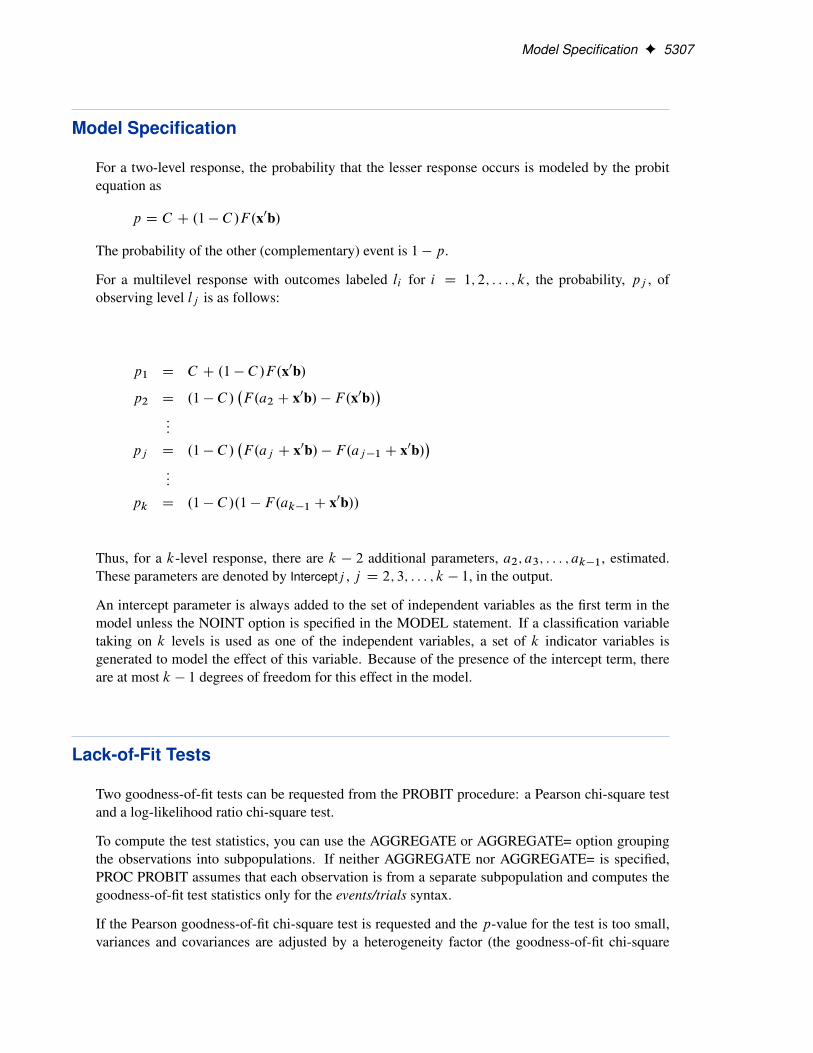
Model Specification F 5307
Model Specification
For a two-level response, the probability that the lesser response occurs is modeled by the probitequation as
p D C C .1 � C /F.x0b/
The probability of the other (complementary) event is 1 � p.
For a multilevel response with outcomes labeled li for i D 1; 2; : : : ; k, the probability, pj , ofobserving level lj is as follows:
p1 D C C .1 � C /F.x0b/
p2 D .1 � C /�F.a2 C x0b/ � F.x0b/
�:::
pj D .1 � C /�F.aj C x0b/ � F.aj �1 C x0b/
�:::
pk D .1 � C /.1 � F.ak�1 C x0b//
Thus, for a k-level response, there are k � 2 additional parameters, a2; a3; : : : ; ak�1, estimated.These parameters are denoted by Interceptj , j D 2; 3; : : : ; k � 1, in the output.
An intercept parameter is always added to the set of independent variables as the first term in themodel unless the NOINT option is specified in the MODEL statement. If a classification variabletaking on k levels is used as one of the independent variables, a set of k indicator variables isgenerated to model the effect of this variable. Because of the presence of the intercept term, thereare at most k � 1 degrees of freedom for this effect in the model.
Lack-of-Fit Tests
Two goodness-of-fit tests can be requested from the PROBIT procedure: a Pearson chi-square testand a log-likelihood ratio chi-square test.
To compute the test statistics, you can use the AGGREGATE or AGGREGATE= option groupingthe observations into subpopulations. If neither AGGREGATE nor AGGREGATE= is specified,PROC PROBIT assumes that each observation is from a separate subpopulation and computes thegoodness-of-fit test statistics only for the events/trials syntax.
If the Pearson goodness-of-fit chi-square test is requested and the p-value for the test is too small,variances and covariances are adjusted by a heterogeneity factor (the goodness-of-fit chi-square
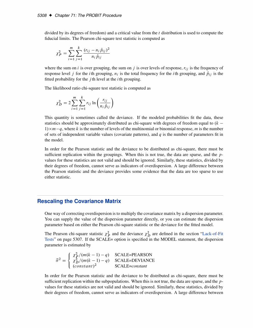
5308 F Chapter 71: The PROBIT Procedure
divided by its degrees of freedom) and a critical value from the t distribution is used to compute thefiducial limits. The Pearson chi-square test statistic is computed as
�2P D
mXiD1
kXj D1
.rij � ni Opij /2
ni Opij
where the sum on i is over grouping, the sum on j is over levels of response, rij is the frequency ofresponse level j for the i th grouping, ni is the total frequency for the i th grouping, and Opij is thefitted probability for the j th level at the i th grouping.
The likelihood ratio chi-square test statistic is computed as
�2D D 2
mXiD1
kXj D1
rij ln�
rij
ni Opij
�
This quantity is sometimes called the deviance. If the modeled probabilities fit the data, thesestatistics should be approximately distributed as chi-square with degrees of freedom equal to .k �
1/�m�q, where k is the number of levels of the multinomial or binomial response, m is the numberof sets of independent variable values (covariate patterns), and q is the number of parameters fit inthe model.
In order for the Pearson statistic and the deviance to be distributed as chi-square, there must besufficient replication within the groupings. When this is not true, the data are sparse, and the p-values for these statistics are not valid and should be ignored. Similarly, these statistics, divided bytheir degrees of freedom, cannot serve as indicators of overdispersion. A large difference betweenthe Pearson statistic and the deviance provides some evidence that the data are too sparse to useeither statistic.
Rescaling the Covariance Matrix
One way of correcting overdispersion is to multiply the covariance matrix by a dispersion parameter.You can supply the value of the dispersion parameter directly, or you can estimate the dispersionparameter based on either the Pearson chi-square statistic or the deviance for the fitted model.
The Pearson chi-square statistic �2P and the deviance �2
D are defined in the section “Lack-of-FitTests” on page 5307. If the SCALE= option is specified in the MODEL statement, the dispersionparameter is estimated by
b�2D
8<:�2
P =.m.k � 1/ � q/ SCALE=PEARSON�2
D=.m.k � 1/ � q/ SCALE=DEVIANCE.constant/2 SCALE=constant
In order for the Pearson statistic and the deviance to be distributed as chi-square, there must besufficient replication within the subpopulations. When this is not true, the data are sparse, and the p-values for these statistics are not valid and should be ignored. Similarly, these statistics, divided bytheir degrees of freedom, cannot serve as indicators of overdispersion. A large difference between
Tolerance Distribution F 5309
the Pearson statistic and the deviance provides some evidence that the data are too sparse to useeither statistic.
You can use the AGGREGATE (or AGGREGATE=) option to define the subpopulation profiles. Ifyou do not specify this option, each observation is regarded as coming from a separate subpopula-tion. For events/trials syntax, each observation represents n Bernoulli trials, where n is the valueof the trials variable; for single-trial syntax, each observation represents a single trial. Without theAGGREGATE (or AGGREGATE=) option, the Pearson chi-square statistic and the deviance arecalculated only for events/trials syntax.
Note that the parameter estimates are not changed by this method. However, their standard errorsare adjusted for overdispersion, affecting their significance tests.
Tolerance Distribution
For a single independent variable, such as a dosage level, the models for the probabilities can bejustified on the basis of a population with mean � and scale parameter � of tolerances for thesubjects. Then, given a dose x, the probability, P , of observing a response in a particular subject isthe probability that the subject’s tolerance is less than the dose or
P D F�x � �
�
�Thus, in this case, the intercept parameter, b0, and the regression parameter, b1, are related to � and� by
b0 D ��
�; b1 D
1
�
NOTE: The parameter � is not equal to the standard deviation of the population of tolerances forthe logistic and extreme value distributions.
Inverse Confidence Limits
In bioassay problems, estimates of the values of the independent variables that yield a desiredresponse are often needed. For instance, the value yielding a 50% response rate (called the ED50or LD50) is often used. The INVERSECL option requests that confidence limits be computed forthe value of the independent variable that yields a specified response. These limits are computedonly for the first continuous variable effect in the model. The other variables are set either at theirmean values if they are continuous or at the reference (last) level if they are discrete variables. Fora discussion of inverse confidence limits, see Hubert, Bohidar, and Peace (1988).
For the PROBIT procedure, the response variable is a probability. An estimate of the first continuousvariable value needed to achieve a response of p is given by
Ox1 D1
b1
�F �1.p/ � x�0b�
�
5310 F Chapter 71: The PROBIT Procedure
where F is the cumulative distribution function used to model the probability, x� is the vectorof independent variables excluding the first one, which can be specified by the XDATA= optiondescribed in the section “XDATA= SAS-data-set” on page 5311, b� is the vector of parameterestimates excluding the first one, and b1 is the estimated regression coefficient for the independentvariable of interest. This estimate assumes that there is no natural response rate (C D 0). When C isnonzero, the quantiles and confidence limits for the independent variable correspond to the adjustedprobability C C.1�C /p, rather than to p. As a result, an estimate of the value yielding response ratep is associated with the .p � C /=.1 � C / quantile. For example, if C D 0:1 then an estimate of theLD50 is found corresponding to the 0.44 quantile. This value can be thought of as yielding 50% ofthe variable’s effect, but a 44% response rate. For both binary and ordinal models, the INVERSECLoption provides estimates of the value of x1, which yields Pr.first response level/ D p, for variousvalues of p.
This estimator is given as a ratio of random variables, such as r D a=b. Confidence limits for thisratio can be computed by using Fieller’s theorem. A brief description of this theorem follows. SeeFinney (1971) for a more complete description of Fieller’s theorem.
If the random variables a and b are thought to be distributed as jointly normal, then for any fixedvalue r the following probability statement holds if z is an ˛=2 quantile from the standard normaldistribution and V is the variance-covariance matrix of a and b:
Pr�.a � rb/2 > z2.Vaa � 2rVab C r2Vbb/
�D ˛
Usually the inequality can be solved for r to yield a confidence interval. The PROBIT procedureuses a value of 1.96 for z, corresponding to an ˛ value of 0.05, unless the goodness-of-fit p-valueis less than the specified value of the HPROB= option. When this happens, the covariance matrix isscaled by the heterogeneity factor, and a t distribution quantile is used for z.
It is possible for the roots of the equation for r to be imaginary or for the confidence interval tobe all points outside of an interval. In these cases, the limits are set to missing by the PROBITprocedure.
Although the normal and logistic distribution give comparable fitted values of p if the empiricallyobserved proportions are not too extreme, they can give appreciably different values when extrapo-lated into the tails. Correspondingly, the estimates of the confidence limits and dose values can bedifferent for the two distributions even when they agree quite well in the body of the data. Extrapo-lation outside of the range of the actual data is often sensitive to model assumptions, and caution isadvised if extrapolation is necessary.
It should be pointed out that, when there is a natural threshold C , the quantiles and confidence limitsfor the independent variable correspond to the adjusted probability C C .1 � C /p.
OUTEST= SAS-data-set
The OUTEST= data set contains parameter estimates and the log likelihood for the model. You canspecify a label in the MODEL statement to distinguish between the estimates for different modelsused by the PROBIT procedure. If you specify the COVOUT option, the OUTEST= data set alsocontains the estimated covariance matrix of the parameter estimates.
XDATA= SAS-data-set F 5311
The OUTEST= data set contains each variable used as a dependent or independent variable in anyMODEL statement. One observation consists of parameter values for the model with the dependentvariable having the value �1. If you specify the COVOUT option, there are additional observationscontaining the rows of the estimated covariance matrix. For these observations, the dependent vari-able contains the parameter estimate for the corresponding row variable. The following variablesare also added to the data set:
_MODEL_ a character variable containing the label of the MODEL statement, if present, orblank otherwise
_NAME_ a character variable containing the name of the dependent variable for the parameterestimates observations or the name of the row for the covariance matrix estimates
_TYPE_ a character variable containing the type of the observation, either PARMS for pa-rameter estimates or COV for covariance estimates
_DIST_ a character variable containing the name of the distribution modeled
_LNLIKE_ a numeric variable containing the last computed value of the log likelihood
_C_ a numeric variable containing the estimated threshold parameter
INTERCEPT a numeric variable containing the intercept parameter estimates and covariances
Any BY variables specified are also added to the OUTEST= data set.
XDATA= SAS-data-set
The XDATA= data set is used for specifying values for the effects in the MODEL statement whenpredicted values and/or fiducial limits for a single continuous variable (dose variable) are required.It is also used for plots specified by the CDFPLOT, IPPPLOT, LPREDPLOT, and PREDPPLOTstatement.
The XDATA= data names a SAS data set that contains user input values for all the independentvariables in the MODEL statement and the variables in the CLASS statement. The XDATA= dataset has the same structure as the DATA= data set but is not required to have all the variables orobservations that appear in the DATA= data set.
The XDATA= data set must contain all the independent variables in the MODEL statement andvariables in the CLASS statement. Even though variables in the CLASS statement are not usedin the MODEL statement, valid values are required for these variables in the XDATA= data set.Missing values are not allowed. For independent variables in the MODEL statement, although thedose variable’s value is not used in the computing of predicted values and/or fiducial limits for thedose variable, missing values are not allowed in the XDATA= data set for any of the independentvariables. Missing values are allowed for the dependent variables and other variables if they areincluded in the XDATA= data set and not listed in the CLASS statement.
If BY processing is used, the XDATA= data set should also include the BY variables, and there mustbe at least one valid observation for each BY group. If there is more than one valid observation inone BY group, the last one read is used for that BY group.
5312 F Chapter 71: The PROBIT Procedure
If there is no XDATA= data set in the PROC PROBIT statement, by default, the PROBIT procedurewill use overall mean for effects containing continuous variable (or variables) and the highest levelof a single classification variable as reference level. The rules are summarized as follows:
� If the effect contains a continuous variable (or variables), the overall mean of this effect isused.
� If the effect is a single classification variable, the highest level of the variable is used.
Traditional High-Resolution Graphics
This section provides examples of using syntax available with the traditional high-resolution plots.There are four plot statements that you can use to request traditional high-resolution plots: CDF-PLOT, IPPPLOT, LPREDPLOT, and PREDPPLOT. Some of these statements apply only to eitherthe binomial model or the multinomial model. Table 71.33 shows the availability of these statementsfor different models.
Table 71.33 Plot Statement Availability
Statement Binomial MultinomialCDFPLOT NO YES
IPPPLOT YES NO
LPREDPLOT YES YES
PREDPPLOT YES YES
An alternative is to use ODS Graphics to obtain these plots. See the section “ODS Graphics” onpage 5319 for details.
The following example uses the data set study in the section “Estimating the Natural ResponseThreshold Parameter” on page 5253 to illustrate how to create high-resolution plots for the binomialmodel:
proc probit data=study log10 optc;model respond/number=dose;predpplot var=dose cfit=blue; inset;lpredplot var=dose cfit=blue; inset;ippplot var=dose cfit=blue; inset/pos=se;
run;
All plot statements must follow the MODEL statement. The VAR= option specifies a continuousindependent variable (dose variable) against which the predicted probability or the linear predictoris plotted. The INSET statement requests the inset box with summary information. See the section“INSET Statement” on page 5271 for more details.
The PREDPPLOT statement creates the plot in Figure 71.6. This plot, similar to that in Figure 71.4,shows the relationship between dosage level, observed response proportions, and estimated prob-ability values. The dashed lines represent pointwise confidence bands for the fitted probabilities,
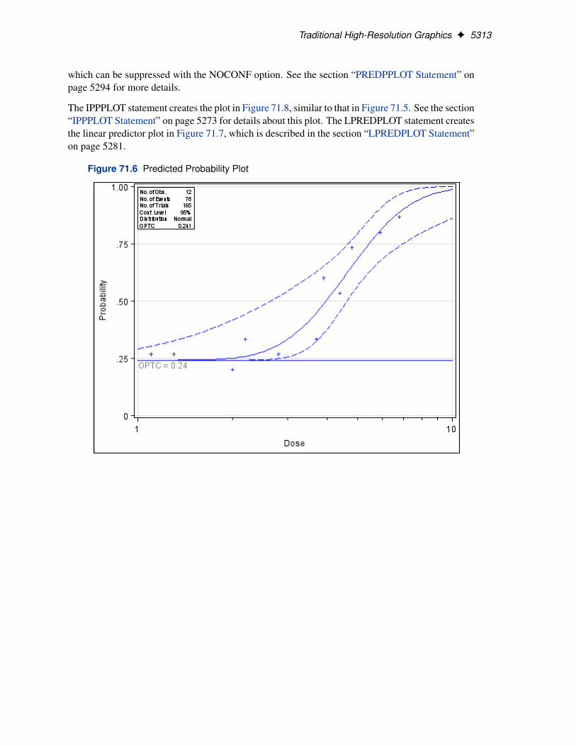
Traditional High-Resolution Graphics F 5313
which can be suppressed with the NOCONF option. See the section “PREDPPLOT Statement” onpage 5294 for more details.
The IPPPLOT statement creates the plot in Figure 71.8, similar to that in Figure 71.5. See the section“IPPPLOT Statement” on page 5273 for details about this plot. The LPREDPLOT statement createsthe linear predictor plot in Figure 71.7, which is described in the section “LPREDPLOT Statement”on page 5281.
Figure 71.6 Predicted Probability Plot
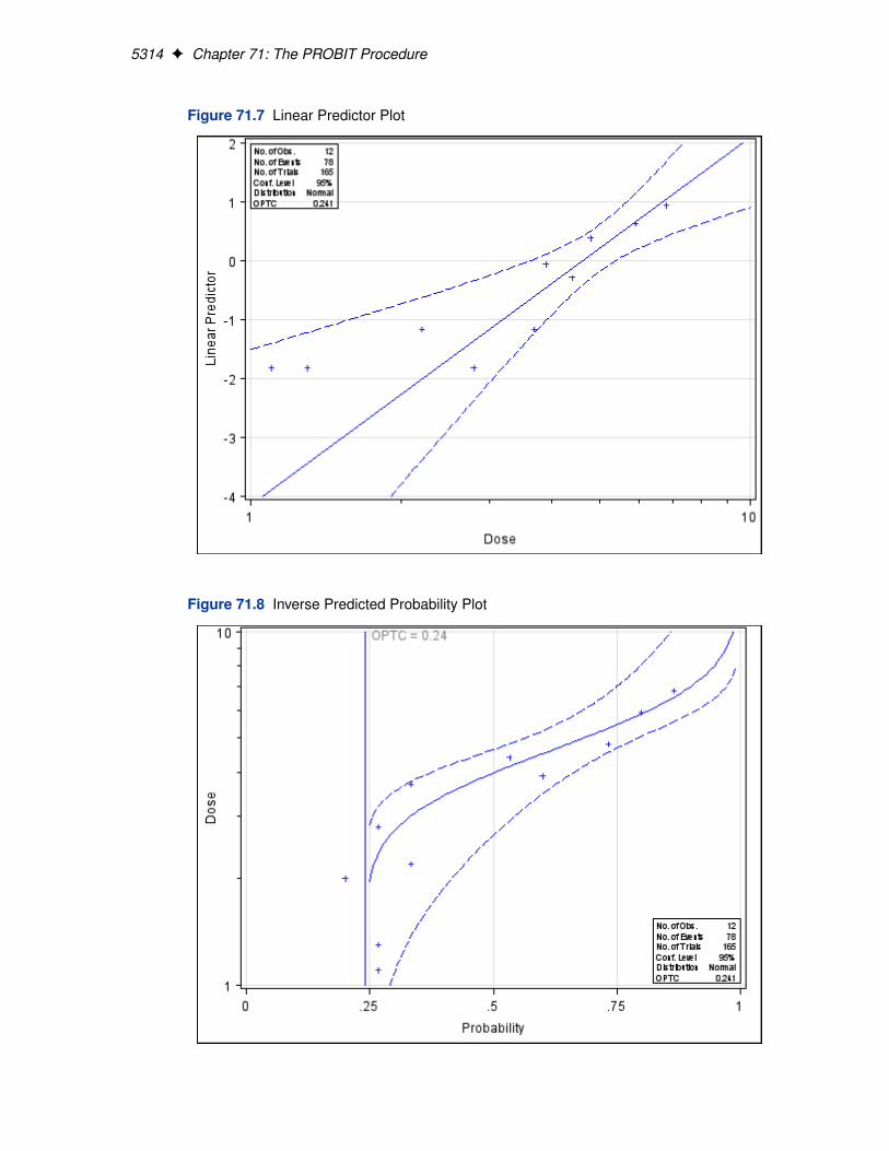
5314 F Chapter 71: The PROBIT Procedure
Figure 71.7 Linear Predictor Plot
Figure 71.8 Inverse Predicted Probability Plot
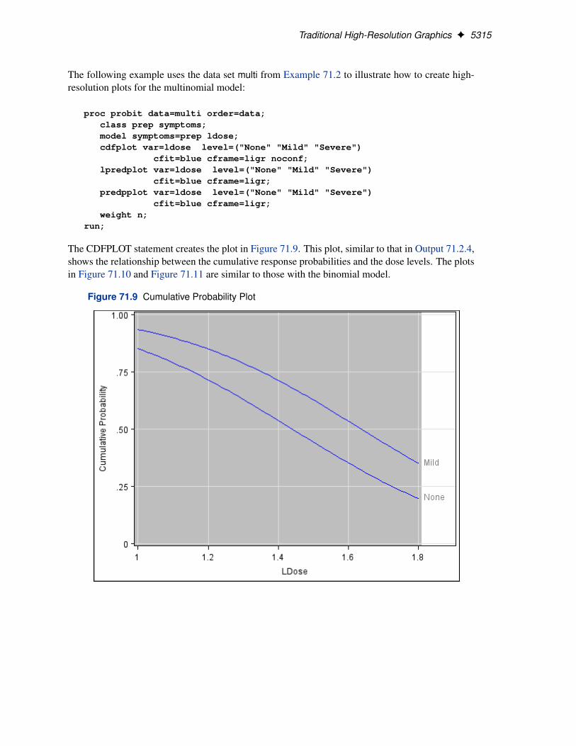
Traditional High-Resolution Graphics F 5315
The following example uses the data set multi from Example 71.2 to illustrate how to create high-resolution plots for the multinomial model:
proc probit data=multi order=data;class prep symptoms;model symptoms=prep ldose;cdfplot var=ldose level=("None" "Mild" "Severe")
cfit=blue cframe=ligr noconf;lpredplot var=ldose level=("None" "Mild" "Severe")
cfit=blue cframe=ligr;predpplot var=ldose level=("None" "Mild" "Severe")
cfit=blue cframe=ligr;weight n;
run;
The CDFPLOT statement creates the plot in Figure 71.9. This plot, similar to that in Output 71.2.4,shows the relationship between the cumulative response probabilities and the dose levels. The plotsin Figure 71.10 and Figure 71.11 are similar to those with the binomial model.
Figure 71.9 Cumulative Probability Plot
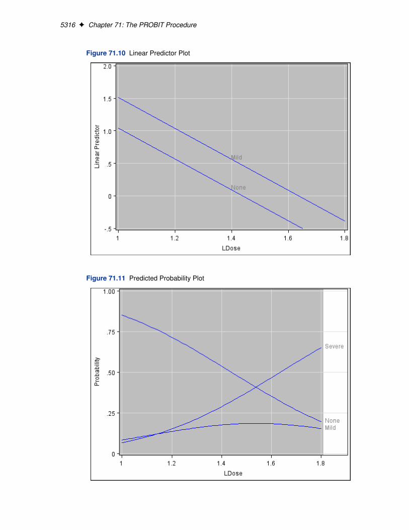
5316 F Chapter 71: The PROBIT Procedure
Figure 71.10 Linear Predictor Plot
Figure 71.11 Predicted Probability Plot
Displayed Output F 5317
Displayed Output
If you request the iteration history (ITPRINT), PROC PROBIT displays the following:
� the current value of the log likelihood
� the ridging parameter for the modified Newton-Raphson optimization process
� the current estimate of the parameters
� the current estimate of the parameter C for a natural (threshold) model
� the values of the gradient and the Hessian on the last iteration
If you include classification variables, PROC PROBIT displays the following:
� the numbers of levels for each classification variable
� the (ordered) values of the levels
� the number of observations used
After the model is fit, PROC PROBIT displays the following:
� the name of the input data set
� the name of the dependent variables
� the number of observations used
� the number of events and the number of trials
� the final value of the log-likelihood function
� the parameter estimates
� the standard error estimates of the parameter estimates
� approximate chi-square test statistics for the test
If you specify the COVB or CORRB options, PROC PROBIT displays the following:
� the estimated covariance matrix for the parameter estimates
� the estimated correlation matrix for the parameter estimates
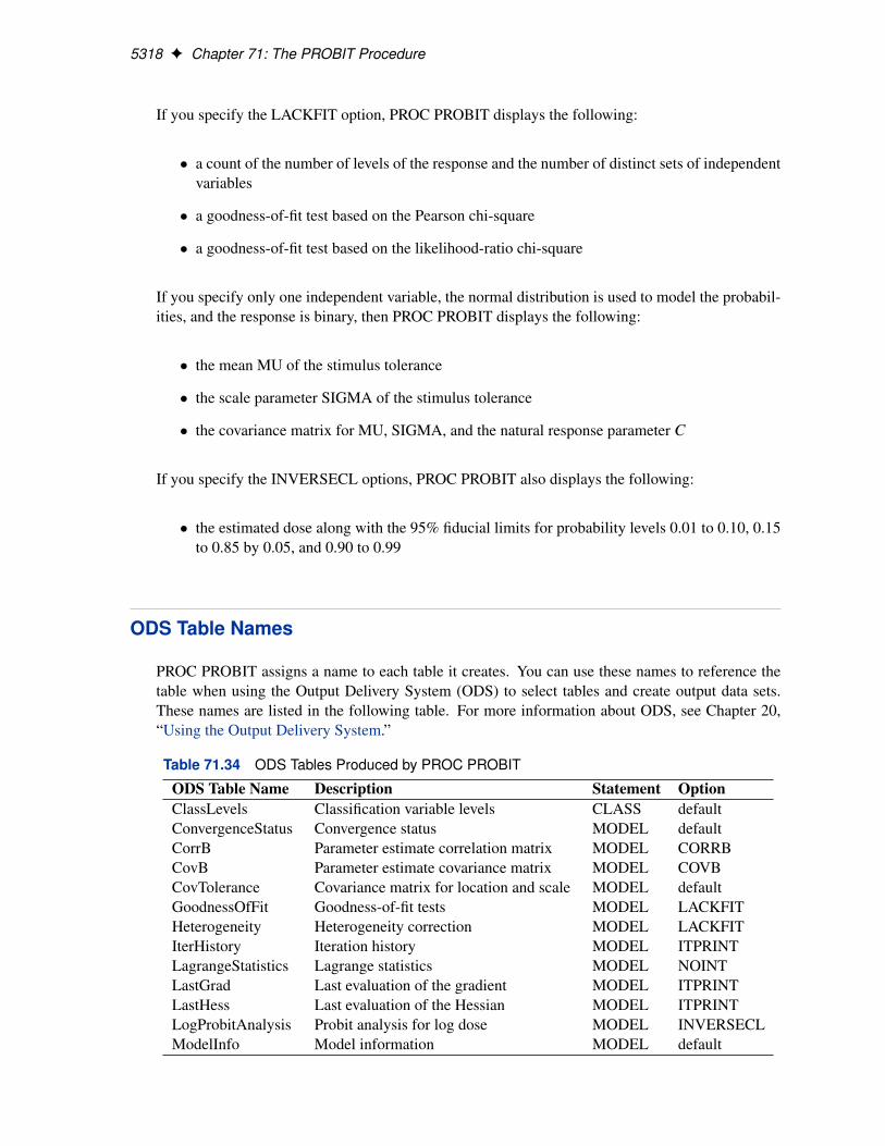
5318 F Chapter 71: The PROBIT Procedure
If you specify the LACKFIT option, PROC PROBIT displays the following:
� a count of the number of levels of the response and the number of distinct sets of independentvariables
� a goodness-of-fit test based on the Pearson chi-square
� a goodness-of-fit test based on the likelihood-ratio chi-square
If you specify only one independent variable, the normal distribution is used to model the probabil-ities, and the response is binary, then PROC PROBIT displays the following:
� the mean MU of the stimulus tolerance
� the scale parameter SIGMA of the stimulus tolerance
� the covariance matrix for MU, SIGMA, and the natural response parameter C
If you specify the INVERSECL options, PROC PROBIT also displays the following:
� the estimated dose along with the 95% fiducial limits for probability levels 0.01 to 0.10, 0.15to 0.85 by 0.05, and 0.90 to 0.99
ODS Table Names
PROC PROBIT assigns a name to each table it creates. You can use these names to reference thetable when using the Output Delivery System (ODS) to select tables and create output data sets.These names are listed in the following table. For more information about ODS, see Chapter 20,“Using the Output Delivery System.”
Table 71.34 ODS Tables Produced by PROC PROBIT
ODS Table Name Description Statement OptionClassLevels Classification variable levels CLASS defaultConvergenceStatus Convergence status MODEL defaultCorrB Parameter estimate correlation matrix MODEL CORRBCovB Parameter estimate covariance matrix MODEL COVBCovTolerance Covariance matrix for location and scale MODEL defaultGoodnessOfFit Goodness-of-fit tests MODEL LACKFITHeterogeneity Heterogeneity correction MODEL LACKFITIterHistory Iteration history MODEL ITPRINTLagrangeStatistics Lagrange statistics MODEL NOINTLastGrad Last evaluation of the gradient MODEL ITPRINTLastHess Last evaluation of the Hessian MODEL ITPRINTLogProbitAnalysis Probit analysis for log dose MODEL INVERSECLModelInfo Model information MODEL default
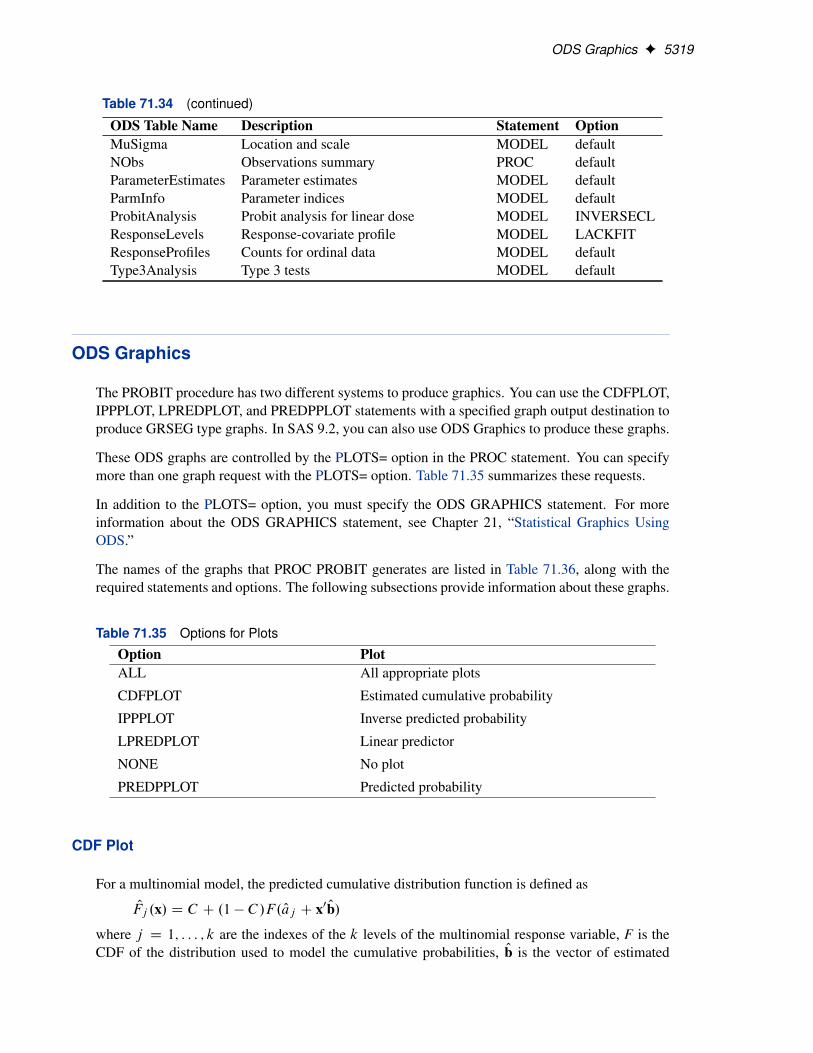
ODS Graphics F 5319
Table 71.34 (continued)
ODS Table Name Description Statement OptionMuSigma Location and scale MODEL defaultNObs Observations summary PROC defaultParameterEstimates Parameter estimates MODEL defaultParmInfo Parameter indices MODEL defaultProbitAnalysis Probit analysis for linear dose MODEL INVERSECLResponseLevels Response-covariate profile MODEL LACKFITResponseProfiles Counts for ordinal data MODEL defaultType3Analysis Type 3 tests MODEL default
ODS Graphics
The PROBIT procedure has two different systems to produce graphics. You can use the CDFPLOT,IPPPLOT, LPREDPLOT, and PREDPPLOT statements with a specified graph output destination toproduce GRSEG type graphs. In SAS 9.2, you can also use ODS Graphics to produce these graphs.
These ODS graphs are controlled by the PLOTS= option in the PROC statement. You can specifymore than one graph request with the PLOTS= option. Table 71.35 summarizes these requests.
In addition to the PLOTS= option, you must specify the ODS GRAPHICS statement. For moreinformation about the ODS GRAPHICS statement, see Chapter 21, “Statistical Graphics UsingODS.”
The names of the graphs that PROC PROBIT generates are listed in Table 71.36, along with therequired statements and options. The following subsections provide information about these graphs.
Table 71.35 Options for Plots
Option PlotALL All appropriate plots
CDFPLOT Estimated cumulative probability
IPPPLOT Inverse predicted probability
LPREDPLOT Linear predictor
NONE No plot
PREDPPLOT Predicted probability
CDF Plot
For a multinomial model, the predicted cumulative distribution function is defined as
OFj .x/ D C C .1 � C /F. Oaj C x0 Ob/
where j D 1; : : : ; k are the indexes of the k levels of the multinomial response variable, F is theCDF of the distribution used to model the cumulative probabilities, Ob is the vector of estimated
5320 F Chapter 71: The PROBIT Procedure
parameters, x is the covariate vector, Oaj are estimated ordinal intercepts with Oa1 D 0, and C
is the threshold parameter, either known or estimated from the model. Let x1 be the covariatecorresponding to the dose variable and x�1 be the vector of the rest of the covariates. Let thecorresponding estimated parameters be Ob1 and Ob�1. Then
OFj .x/ D C C .1 � C /F. Oaj C x1Ob1 C x0
�1Ob�1/
To plot OFj as a function of x1, x�1 must be specified. You can use the XDATA= option to providethe values of x�1 (see the XDATA= option in the PROC PROBIT statement for details), or use thedefault values that follow these rules:
� If the effect contains a continuous variable (or variables), the overall mean of this effect isused.
� If the effect is a single classification variable, the highest level of the variable is used.
The LEVEL= suboption specify the levels of the multinomial response variable for which the CDFcurves are requested. There are k � 1 curves for a k-level multinomial response variable (for thehighest level, it is the constant line 1). You can specify any of them to be plotted by the LEVEL=suboption. See the plot in Output 71.2.6 for an example.
Inverse Predicted Probability Plot
For the binomial model, the response variable is a probability. An estimate of the dose level Ox1
needed for a response of p is given by
Ox1 D .F �1.p/ � x0�1
Ob�1/= Ob1
where F is the cumulative distribution function used to model the probability, x�1 is the vector ofthe rest of the covariates, Ob�1 is the vector of the estimated parameters corresponding to x�1, andOb1 is the estimated parameter for the dose variable of interest.
To plot Ox1 as a function of p, x�1 must be specified. You can use the XDATA= option to providethe values of x�1 (see the XDATA= option in the PROC PROBIT statement for details), or use thedefault values that follow these rules:
� If the effect contains a continuous variable (or variables), the overall mean of this effect isused.
� If the effect is a single classification variable, the highest level of the variable is used.
Output 71.4.12 in Example 71.4 shows an inverse predicted probability plot.
ODS Graphics F 5321
Linear Predictor Plot
For both binomial models and multinomial models, the linear predictor x0b can be plotted againstthe first single continuous variable (dose variable) in the MODEL statement.
Let x1 be the covariate of the dose variable, x�1 be the vector of the rest of the covariates, Ob�1 bethe vector of estimated parameters corresponding to x�1, and Ob1 be the estimated parameter for thedose variable of interest.
To plot Ox0b as a function of x1, x�1 must be specified. You can use the XDATA= option to providethe values of x�1 (see the XDATA= option in the PROC PROBIT statement for details), or use thedefault values that follow these rules:
� If the effect contains a continuous variable (or variables), the overall mean of this effect isused.
� If the effect is a single classification variable, the highest level of the variable is used.
For the multinomial model, you can use the LEVEL= suboption to specify the levels for which thelinear predictor lines are plotted.
The confidence limits for the predicted values are only available for the binomial model.Output 71.4.13 in Example 71.4 shows a linear predictor plot for a binomial model.
Predicted Probability Plot
The predicted probability is
Op D C C .1 � C /F.x0 Ob/
for the binomial model and
Op1 D C C .1 � C /F.x0 Ob/
Opj D .1 � C /.F. Oaj C x0 Ob/ � F. Oaj �1 C x0 Ob//; j D 2; : : : ; k � 1
Opk D .1 � C /.1 � F. Oak�1 C x0 Ob//
for the multinomial model with k response levels, where F is the cumulative distribution functionused to model the probability, x0 is the vector of the covariates, Oaj are the estimated ordinal inter-cepts with Oa1 D 0, C is the threshold parameter, either known or estimated from the model, and Ob0
is the vector of estimated parameters.
To plot Op (or Opj ) as a function of a continuous variable x1, the remaining covariates x�1 must bespecified. You can use the XDATA= option to provide the values of x�1 (see the XDATA= optionin the PROC PROBIT statement for details), or use the default values that follow these rules:
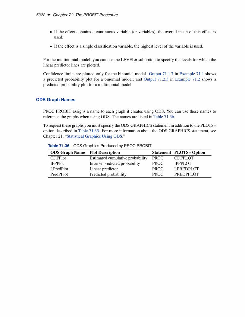
5322 F Chapter 71: The PROBIT Procedure
� If the effect contains a continuous variable (or variables), the overall mean of this effect isused.
� If the effect is a single classification variable, the highest level of the variable is used.
For the multinomial model, you can use the LEVEL= suboption to specify the levels for which thelinear predictor lines are plotted.
Confidence limits are plotted only for the binomial model. Output 71.1.7 in Example 71.1 showsa predicted probability plot for a binomial model; and Output 71.2.3 in Example 71.2 shows apredicted probability plot for a multinomial model.
ODS Graph Names
PROC PROBIT assigns a name to each graph it creates using ODS. You can use these names toreference the graphs when using ODS. The names are listed in Table 71.36.
To request these graphs you must specify the ODS GRAPHICS statement in addition to the PLOTS=option described in Table 71.35. For more information about the ODS GRAPHICS statement, seeChapter 21, “Statistical Graphics Using ODS.”
Table 71.36 ODS Graphics Produced by PROC PROBIT
ODS Graph Name Plot Description Statement PLOTS= OptionCDFPlot Estimated cumulative probability PROC CDFPLOTIPPPlot Inverse predicted probability PROC IPPPLOTLPredPlot Linear predictor PROC LPREDPLOTPredPPlot Predicted probability PROC PREDPPLOT
Examples: PROBIT Procedure F 5323
Examples: PROBIT Procedure
Example 71.1: Dosage Levels
In this example, Dose is a variable representing the level of a stimulus, N represents the number ofsubjects tested at each level of the stimulus, and Response is the number of subjects responding tothat level of the stimulus. Both probit and logit response models are fit to the data. The LOG10option in the PROC PROBIT statement requests that the log base 10 of Dose is used as the inde-pendent variable. Specifically, for a given level of Dose, the probability p of a positive response ismodeled as
p D Pr.Response/ D F .b0 C b1 � log10.Dose//
The probabilities are estimated first by using the normal distribution function (the default) and thenby using the logistic distribution function. Note that, in this model specification, the natural rate isassumed to be zero.
The LACKFIT option specifies lack-of-fit tests and the INVERSECL option specifies inverse con-fidence limits.
In the DATA step that reads the data, a number of observations are generated that have a missingvalue for the response. Although the PROBIT procedure does not use the observations with themissing values to fit the model, it does give predicted values for all nonmissing sets of independentvariables. These data points fill in the plot of fitted and observed values in the logistic modeldisplayed in Output 71.1.7. The plot, requested with the PLOT=PREDPPLOT option, displays theestimated logistic cumulative distribution function and the observed response rates.
The following statements produce Output 71.1.1:data a;
infile cards eof=eof;input Dose N Response @@;Observed= Response/N;output;return;
eof: do Dose=0.5 to 7.5 by 0.25;output;
end;datalines;
1 10 1 2 12 2 3 10 4 4 10 55 12 8 6 10 8 7 10 10;
proc probit log10;model Response/N=Dose / lackfit inversecl itprint;output out=B p=Prob std=std xbeta=xbeta;
run;
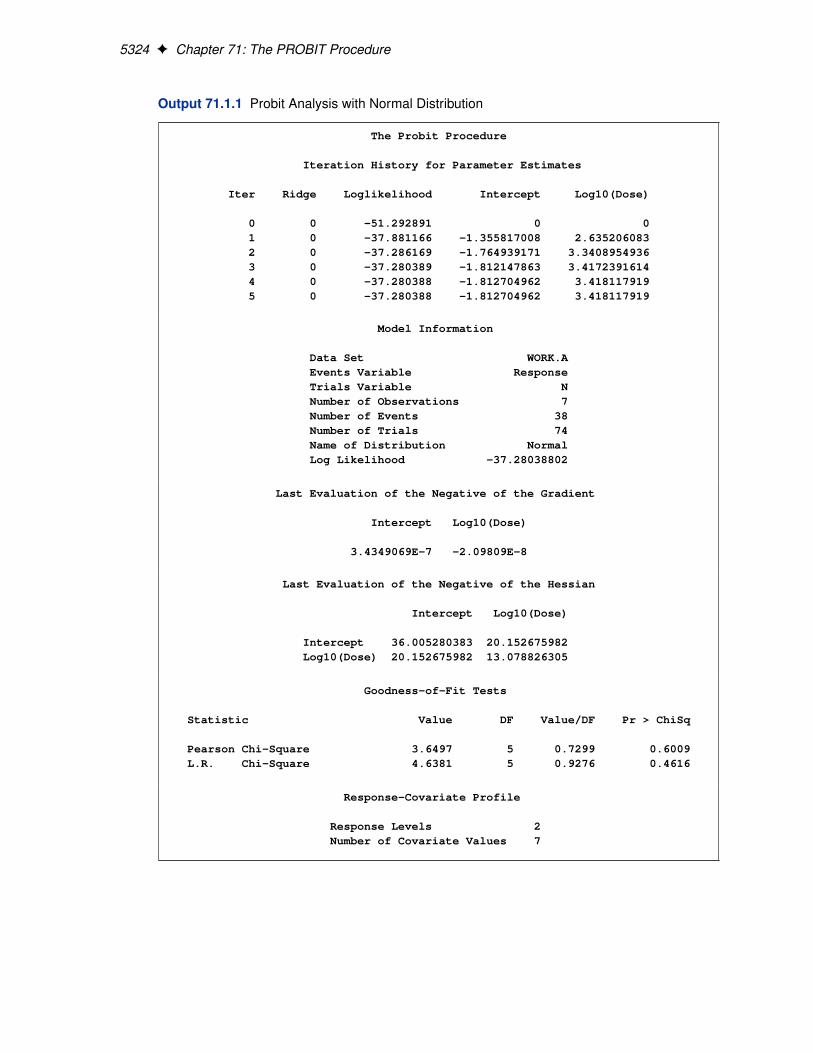
5324 F Chapter 71: The PROBIT Procedure
Output 71.1.1 Probit Analysis with Normal Distribution
The Probit Procedure
Iteration History for Parameter Estimates
Iter Ridge Loglikelihood Intercept Log10(Dose)
0 0 -51.292891 0 01 0 -37.881166 -1.355817008 2.6352060832 0 -37.286169 -1.764939171 3.34089549363 0 -37.280389 -1.812147863 3.41723916144 0 -37.280388 -1.812704962 3.4181179195 0 -37.280388 -1.812704962 3.418117919
Model Information
Data Set WORK.AEvents Variable ResponseTrials Variable NNumber of Observations 7Number of Events 38Number of Trials 74Name of Distribution NormalLog Likelihood -37.28038802
Last Evaluation of the Negative of the Gradient
Intercept Log10(Dose)
3.4349069E-7 -2.09809E-8
Last Evaluation of the Negative of the Hessian
Intercept Log10(Dose)
Intercept 36.005280383 20.152675982Log10(Dose) 20.152675982 13.078826305
Goodness-of-Fit Tests
Statistic Value DF Value/DF Pr > ChiSq
Pearson Chi-Square 3.6497 5 0.7299 0.6009L.R. Chi-Square 4.6381 5 0.9276 0.4616
Response-Covariate Profile
Response Levels 2Number of Covariate Values 7
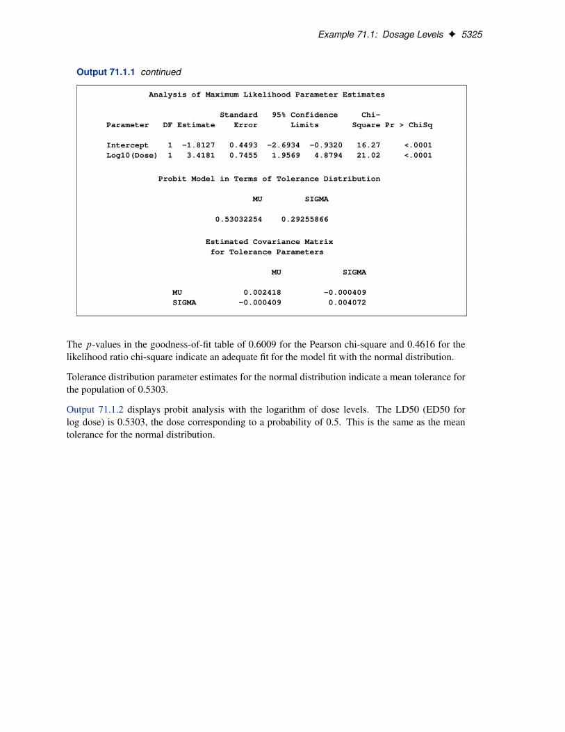
Example 71.1: Dosage Levels F 5325
Output 71.1.1 continued
Analysis of Maximum Likelihood Parameter Estimates
Standard 95% Confidence Chi-Parameter DF Estimate Error Limits Square Pr > ChiSq
Intercept 1 -1.8127 0.4493 -2.6934 -0.9320 16.27 <.0001Log10(Dose) 1 3.4181 0.7455 1.9569 4.8794 21.02 <.0001
Probit Model in Terms of Tolerance Distribution
MU SIGMA
0.53032254 0.29255866
Estimated Covariance Matrixfor Tolerance Parameters
MU SIGMA
MU 0.002418 -0.000409SIGMA -0.000409 0.004072
The p-values in the goodness-of-fit table of 0.6009 for the Pearson chi-square and 0.4616 for thelikelihood ratio chi-square indicate an adequate fit for the model fit with the normal distribution.
Tolerance distribution parameter estimates for the normal distribution indicate a mean tolerance forthe population of 0.5303.
Output 71.1.2 displays probit analysis with the logarithm of dose levels. The LD50 (ED50 forlog dose) is 0.5303, the dose corresponding to a probability of 0.5. This is the same as the meantolerance for the normal distribution.
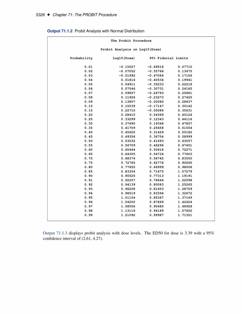
5326 F Chapter 71: The PROBIT Procedure
Output 71.1.2 Probit Analysis with Normal Distribution
The Probit Procedure
Probit Analysis on Log10(Dose)
Probability Log10(Dose) 95% Fiducial Limits
0.01 -0.15027 -0.69518 0.077100.02 -0.07052 -0.55766 0.134750.03 -0.01992 -0.47064 0.171560.04 0.01814 -0.40534 0.199410.05 0.04911 -0.35233 0.222180.06 0.07546 -0.30731 0.241650.07 0.09857 -0.26793 0.258810.08 0.11926 -0.23273 0.274250.09 0.13807 -0.20080 0.288370.10 0.15539 -0.17147 0.301420.15 0.22710 -0.05086 0.356310.20 0.28410 0.04369 0.401240.25 0.33299 0.12343 0.441160.30 0.37690 0.19348 0.478570.35 0.41759 0.25658 0.515040.40 0.45620 0.31429 0.551820.45 0.49356 0.36754 0.589990.50 0.53032 0.41693 0.630570.55 0.56709 0.46296 0.674510.60 0.60444 0.50618 0.722710.65 0.64305 0.54734 0.776030.70 0.68374 0.58745 0.835500.75 0.72765 0.62776 0.902650.80 0.77655 0.66999 0.980080.85 0.83354 0.71675 1.072790.90 0.90525 0.77313 1.191910.91 0.92257 0.78646 1.220980.92 0.94139 0.80083 1.252650.93 0.96208 0.81653 1.287590.94 0.98519 0.83394 1.326720.95 1.01154 0.85367 1.371490.96 1.04250 0.87669 1.424240.97 1.08056 0.90480 1.489280.98 1.13116 0.94189 1.576020.99 1.21092 0.99987 1.71321
Output 71.1.3 displays probit analysis with dose levels. The ED50 for dose is 3.39 with a 95%confidence interval of (2.61, 4.27).
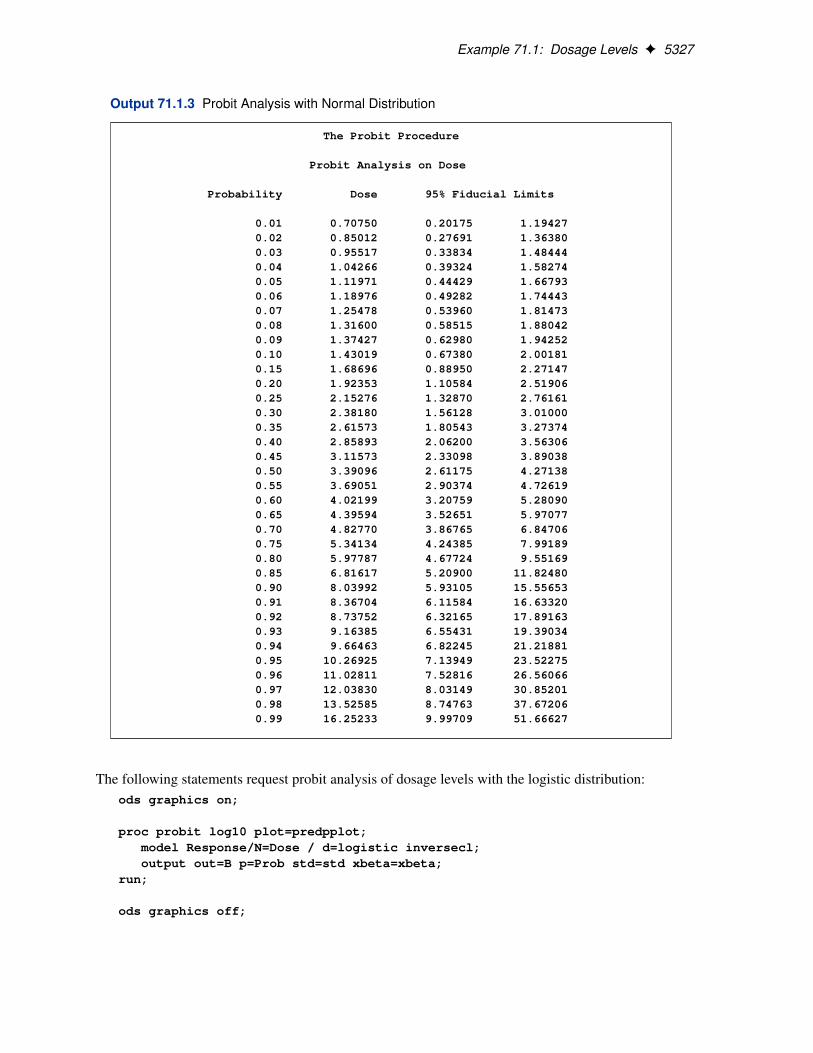
Example 71.1: Dosage Levels F 5327
Output 71.1.3 Probit Analysis with Normal Distribution
The Probit Procedure
Probit Analysis on Dose
Probability Dose 95% Fiducial Limits
0.01 0.70750 0.20175 1.194270.02 0.85012 0.27691 1.363800.03 0.95517 0.33834 1.484440.04 1.04266 0.39324 1.582740.05 1.11971 0.44429 1.667930.06 1.18976 0.49282 1.744430.07 1.25478 0.53960 1.814730.08 1.31600 0.58515 1.880420.09 1.37427 0.62980 1.942520.10 1.43019 0.67380 2.001810.15 1.68696 0.88950 2.271470.20 1.92353 1.10584 2.519060.25 2.15276 1.32870 2.761610.30 2.38180 1.56128 3.010000.35 2.61573 1.80543 3.273740.40 2.85893 2.06200 3.563060.45 3.11573 2.33098 3.890380.50 3.39096 2.61175 4.271380.55 3.69051 2.90374 4.726190.60 4.02199 3.20759 5.280900.65 4.39594 3.52651 5.970770.70 4.82770 3.86765 6.847060.75 5.34134 4.24385 7.991890.80 5.97787 4.67724 9.551690.85 6.81617 5.20900 11.824800.90 8.03992 5.93105 15.556530.91 8.36704 6.11584 16.633200.92 8.73752 6.32165 17.891630.93 9.16385 6.55431 19.390340.94 9.66463 6.82245 21.218810.95 10.26925 7.13949 23.522750.96 11.02811 7.52816 26.560660.97 12.03830 8.03149 30.852010.98 13.52585 8.74763 37.672060.99 16.25233 9.99709 51.66627
The following statements request probit analysis of dosage levels with the logistic distribution:ods graphics on;
proc probit log10 plot=predpplot;model Response/N=Dose / d=logistic inversecl;output out=B p=Prob std=std xbeta=xbeta;
run;
ods graphics off;
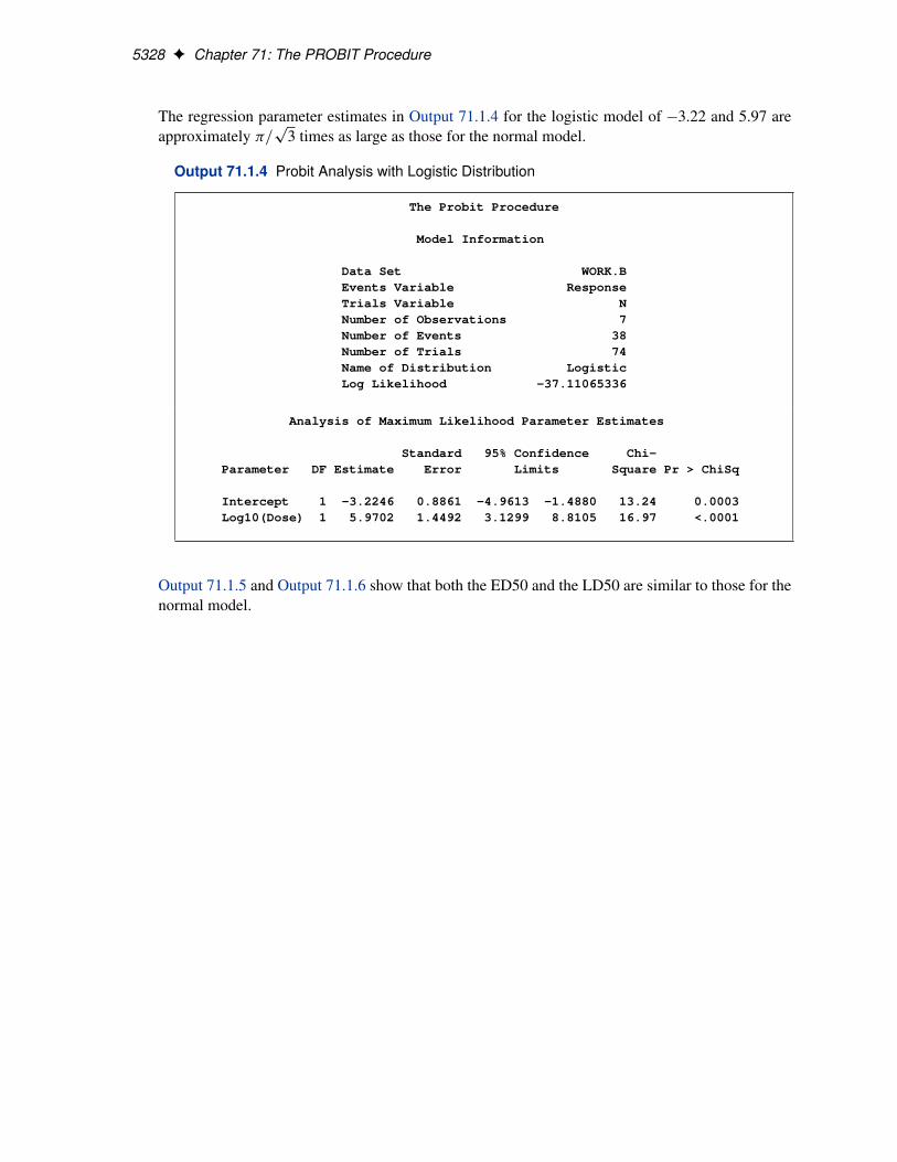
5328 F Chapter 71: The PROBIT Procedure
The regression parameter estimates in Output 71.1.4 for the logistic model of �3.22 and 5.97 areapproximately �=
p3 times as large as those for the normal model.
Output 71.1.4 Probit Analysis with Logistic Distribution
The Probit Procedure
Model Information
Data Set WORK.BEvents Variable ResponseTrials Variable NNumber of Observations 7Number of Events 38Number of Trials 74Name of Distribution LogisticLog Likelihood -37.11065336
Analysis of Maximum Likelihood Parameter Estimates
Standard 95% Confidence Chi-Parameter DF Estimate Error Limits Square Pr > ChiSq
Intercept 1 -3.2246 0.8861 -4.9613 -1.4880 13.24 0.0003Log10(Dose) 1 5.9702 1.4492 3.1299 8.8105 16.97 <.0001
Output 71.1.5 and Output 71.1.6 show that both the ED50 and the LD50 are similar to those for thenormal model.
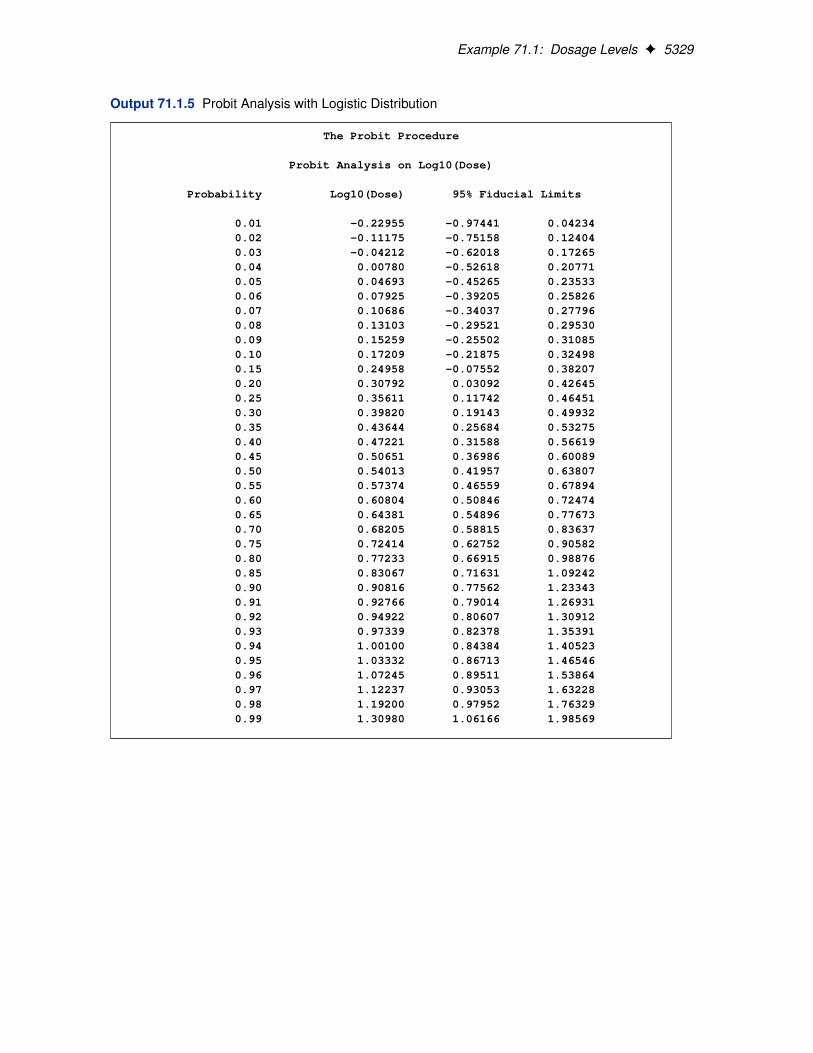
Example 71.1: Dosage Levels F 5329
Output 71.1.5 Probit Analysis with Logistic Distribution
The Probit Procedure
Probit Analysis on Log10(Dose)
Probability Log10(Dose) 95% Fiducial Limits
0.01 -0.22955 -0.97441 0.042340.02 -0.11175 -0.75158 0.124040.03 -0.04212 -0.62018 0.172650.04 0.00780 -0.52618 0.207710.05 0.04693 -0.45265 0.235330.06 0.07925 -0.39205 0.258260.07 0.10686 -0.34037 0.277960.08 0.13103 -0.29521 0.295300.09 0.15259 -0.25502 0.310850.10 0.17209 -0.21875 0.324980.15 0.24958 -0.07552 0.382070.20 0.30792 0.03092 0.426450.25 0.35611 0.11742 0.464510.30 0.39820 0.19143 0.499320.35 0.43644 0.25684 0.532750.40 0.47221 0.31588 0.566190.45 0.50651 0.36986 0.600890.50 0.54013 0.41957 0.638070.55 0.57374 0.46559 0.678940.60 0.60804 0.50846 0.724740.65 0.64381 0.54896 0.776730.70 0.68205 0.58815 0.836370.75 0.72414 0.62752 0.905820.80 0.77233 0.66915 0.988760.85 0.83067 0.71631 1.092420.90 0.90816 0.77562 1.233430.91 0.92766 0.79014 1.269310.92 0.94922 0.80607 1.309120.93 0.97339 0.82378 1.353910.94 1.00100 0.84384 1.405230.95 1.03332 0.86713 1.465460.96 1.07245 0.89511 1.538640.97 1.12237 0.93053 1.632280.98 1.19200 0.97952 1.763290.99 1.30980 1.06166 1.98569
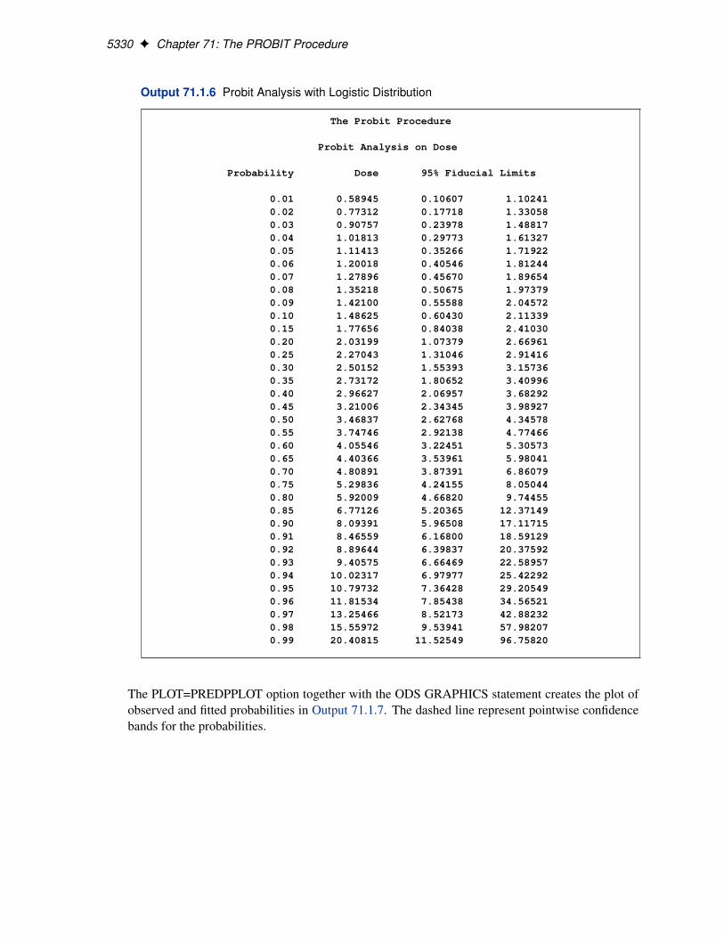
5330 F Chapter 71: The PROBIT Procedure
Output 71.1.6 Probit Analysis with Logistic Distribution
The Probit Procedure
Probit Analysis on Dose
Probability Dose 95% Fiducial Limits
0.01 0.58945 0.10607 1.102410.02 0.77312 0.17718 1.330580.03 0.90757 0.23978 1.488170.04 1.01813 0.29773 1.613270.05 1.11413 0.35266 1.719220.06 1.20018 0.40546 1.812440.07 1.27896 0.45670 1.896540.08 1.35218 0.50675 1.973790.09 1.42100 0.55588 2.045720.10 1.48625 0.60430 2.113390.15 1.77656 0.84038 2.410300.20 2.03199 1.07379 2.669610.25 2.27043 1.31046 2.914160.30 2.50152 1.55393 3.157360.35 2.73172 1.80652 3.409960.40 2.96627 2.06957 3.682920.45 3.21006 2.34345 3.989270.50 3.46837 2.62768 4.345780.55 3.74746 2.92138 4.774660.60 4.05546 3.22451 5.305730.65 4.40366 3.53961 5.980410.70 4.80891 3.87391 6.860790.75 5.29836 4.24155 8.050440.80 5.92009 4.66820 9.744550.85 6.77126 5.20365 12.371490.90 8.09391 5.96508 17.117150.91 8.46559 6.16800 18.591290.92 8.89644 6.39837 20.375920.93 9.40575 6.66469 22.589570.94 10.02317 6.97977 25.422920.95 10.79732 7.36428 29.205490.96 11.81534 7.85438 34.565210.97 13.25466 8.52173 42.882320.98 15.55972 9.53941 57.982070.99 20.40815 11.52549 96.75820
The PLOT=PREDPPLOT option together with the ODS GRAPHICS statement creates the plot ofobserved and fitted probabilities in Output 71.1.7. The dashed line represent pointwise confidencebands for the probabilities.
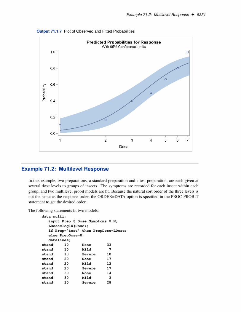
Example 71.2: Multilevel Response F 5331
Output 71.1.7 Plot of Observed and Fitted Probabilities
Example 71.2: Multilevel Response
In this example, two preparations, a standard preparation and a test preparation, are each given atseveral dose levels to groups of insects. The symptoms are recorded for each insect within eachgroup, and two multilevel probit models are fit. Because the natural sort order of the three levels isnot the same as the response order, the ORDER=DATA option is specified in the PROC PROBITstatement to get the desired order.
The following statements fit two models:data multi;
input Prep $ Dose Symptoms $ N;LDose=log10(Dose);if Prep=’test’ then PrepDose=LDose;else PrepDose=0;datalines;
stand 10 None 33stand 10 Mild 7stand 10 Severe 10stand 20 None 17stand 20 Mild 13stand 20 Severe 17stand 30 None 14stand 30 Mild 3stand 30 Severe 28
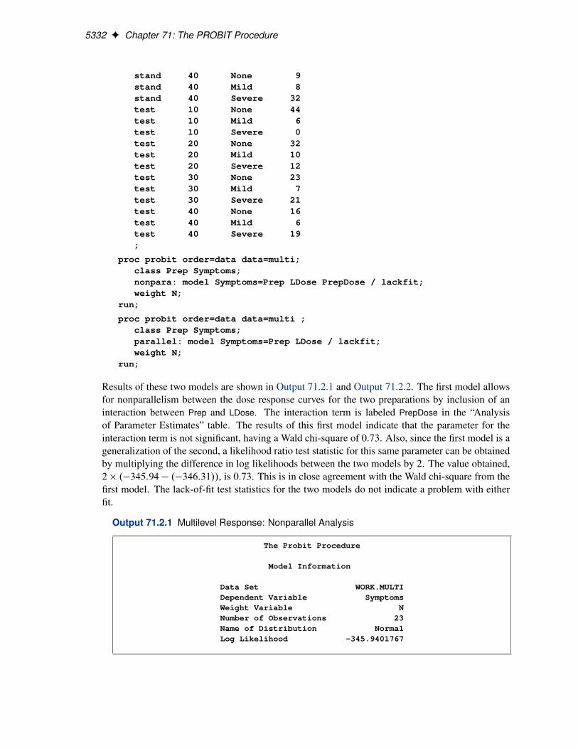
5332 F Chapter 71: The PROBIT Procedure
stand 40 None 9stand 40 Mild 8stand 40 Severe 32test 10 None 44test 10 Mild 6test 10 Severe 0test 20 None 32test 20 Mild 10test 20 Severe 12test 30 None 23test 30 Mild 7test 30 Severe 21test 40 None 16test 40 Mild 6test 40 Severe 19;
proc probit order=data data=multi;class Prep Symptoms;nonpara: model Symptoms=Prep LDose PrepDose / lackfit;weight N;
run;
proc probit order=data data=multi ;class Prep Symptoms;parallel: model Symptoms=Prep LDose / lackfit;weight N;
run;
Results of these two models are shown in Output 71.2.1 and Output 71.2.2. The first model allowsfor nonparallelism between the dose response curves for the two preparations by inclusion of aninteraction between Prep and LDose. The interaction term is labeled PrepDose in the “Analysisof Parameter Estimates” table. The results of this first model indicate that the parameter for theinteraction term is not significant, having a Wald chi-square of 0.73. Also, since the first model is ageneralization of the second, a likelihood ratio test statistic for this same parameter can be obtainedby multiplying the difference in log likelihoods between the two models by 2. The value obtained,2 � .�345:94 � .�346:31//, is 0.73. This is in close agreement with the Wald chi-square from thefirst model. The lack-of-fit test statistics for the two models do not indicate a problem with eitherfit.
Output 71.2.1 Multilevel Response: Nonparallel Analysis
The Probit Procedure
Model Information
Data Set WORK.MULTIDependent Variable SymptomsWeight Variable NNumber of Observations 23Name of Distribution NormalLog Likelihood -345.9401767
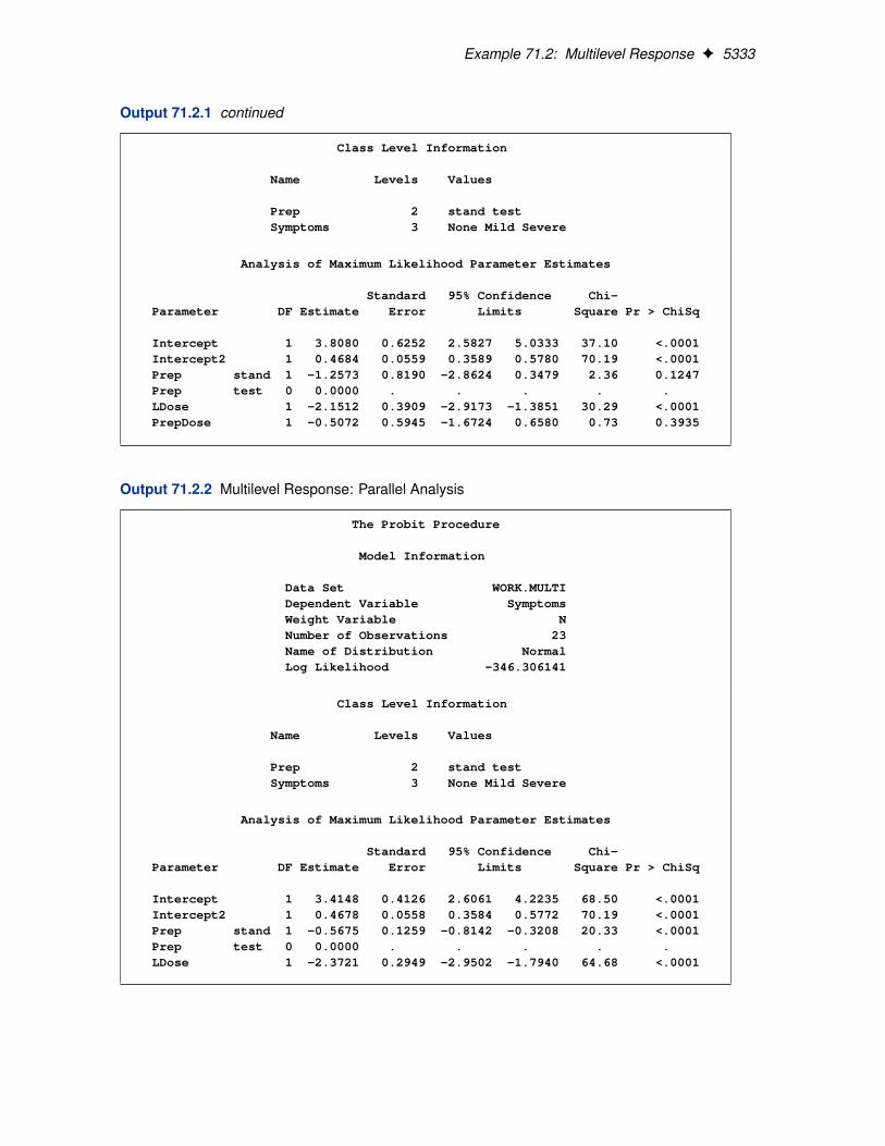
Example 71.2: Multilevel Response F 5333
Output 71.2.1 continued
Class Level Information
Name Levels Values
Prep 2 stand testSymptoms 3 None Mild Severe
Analysis of Maximum Likelihood Parameter Estimates
Standard 95% Confidence Chi-Parameter DF Estimate Error Limits Square Pr > ChiSq
Intercept 1 3.8080 0.6252 2.5827 5.0333 37.10 <.0001Intercept2 1 0.4684 0.0559 0.3589 0.5780 70.19 <.0001Prep stand 1 -1.2573 0.8190 -2.8624 0.3479 2.36 0.1247Prep test 0 0.0000 . . . . .LDose 1 -2.1512 0.3909 -2.9173 -1.3851 30.29 <.0001PrepDose 1 -0.5072 0.5945 -1.6724 0.6580 0.73 0.3935
Output 71.2.2 Multilevel Response: Parallel Analysis
The Probit Procedure
Model Information
Data Set WORK.MULTIDependent Variable SymptomsWeight Variable NNumber of Observations 23Name of Distribution NormalLog Likelihood -346.306141
Class Level Information
Name Levels Values
Prep 2 stand testSymptoms 3 None Mild Severe
Analysis of Maximum Likelihood Parameter Estimates
Standard 95% Confidence Chi-Parameter DF Estimate Error Limits Square Pr > ChiSq
Intercept 1 3.4148 0.4126 2.6061 4.2235 68.50 <.0001Intercept2 1 0.4678 0.0558 0.3584 0.5772 70.19 <.0001Prep stand 1 -0.5675 0.1259 -0.8142 -0.3208 20.33 <.0001Prep test 0 0.0000 . . . . .LDose 1 -2.3721 0.2949 -2.9502 -1.7940 64.68 <.0001
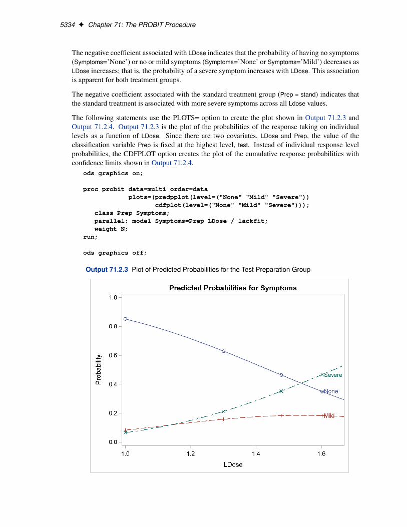
5334 F Chapter 71: The PROBIT Procedure
The negative coefficient associated with LDose indicates that the probability of having no symptoms(Symptoms=’None’) or no or mild symptoms (Symptoms=’None’ or Symptoms=’Mild’) decreases asLDose increases; that is, the probability of a severe symptom increases with LDose. This associationis apparent for both treatment groups.
The negative coefficient associated with the standard treatment group (Prep = stand) indicates thatthe standard treatment is associated with more severe symptoms across all Ldose values.
The following statements use the PLOTS= option to create the plot shown in Output 71.2.3 andOutput 71.2.4. Output 71.2.3 is the plot of the probabilities of the response taking on individuallevels as a function of LDose. Since there are two covariates, LDose and Prep, the value of theclassification variable Prep is fixed at the highest level, test. Instead of individual response levelprobabilities, the CDFPLOT option creates the plot of the cumulative response probabilities withconfidence limits shown in Output 71.2.4.
ods graphics on;
proc probit data=multi order=dataplots=(predpplot(level=("None" "Mild" "Severe"))
cdfplot(level=("None" "Mild" "Severe")));class Prep Symptoms;parallel: model Symptoms=Prep LDose / lackfit;weight N;
run;
ods graphics off;
Output 71.2.3 Plot of Predicted Probabilities for the Test Preparation Group
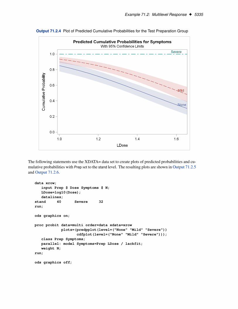
Example 71.2: Multilevel Response F 5335
Output 71.2.4 Plot of Predicted Cumulative Probabilities for the Test Preparation Group
The following statements use the XDATA= data set to create plots of predicted probabilities and cu-mulative probabilities with Prep set to the stand level. The resulting plots are shown in Output 71.2.5and Output 71.2.6.
data xrow;input Prep $ Dose Symptoms $ N;LDose=log10(Dose);datalines;
stand 40 Severe 32run;
ods graphics on;
proc probit data=multi order=data xdata=xrowplots=(predpplot(level=("None" "Mild" "Severe"))
cdfplot(level=("None" "Mild" "Severe")));class Prep Symptoms;parallel: model Symptoms=Prep LDose / lackfit;weight N;
run;
ods graphics off;
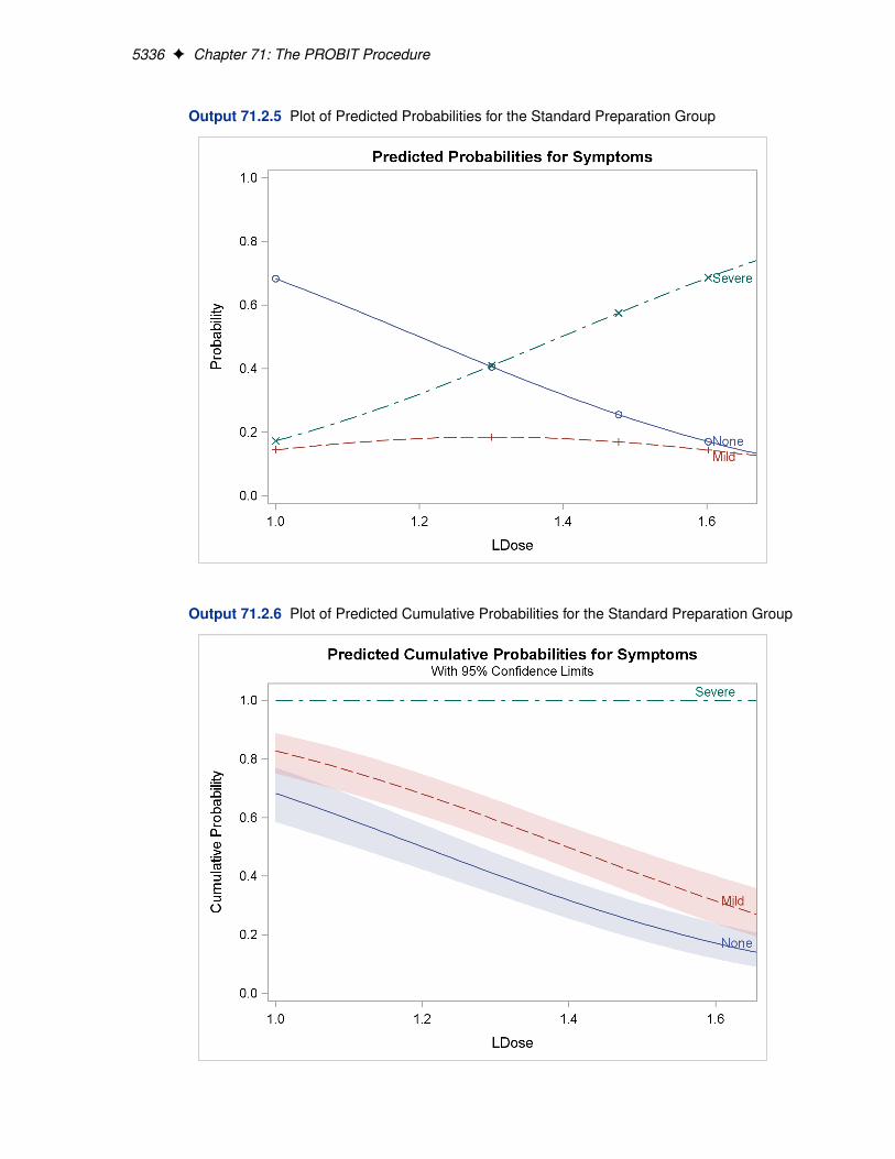
5336 F Chapter 71: The PROBIT Procedure
Output 71.2.5 Plot of Predicted Probabilities for the Standard Preparation Group
Output 71.2.6 Plot of Predicted Cumulative Probabilities for the Standard Preparation Group
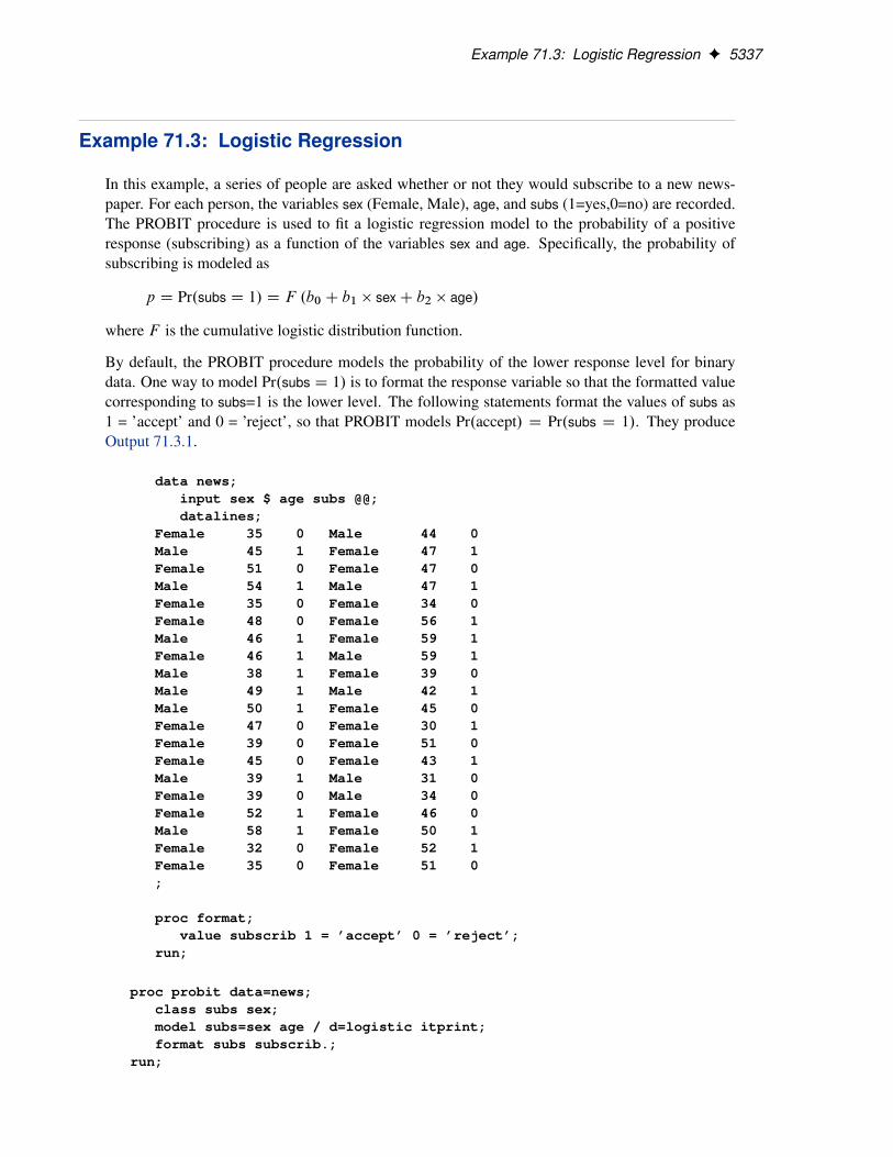
Example 71.3: Logistic Regression F 5337
Example 71.3: Logistic Regression
In this example, a series of people are asked whether or not they would subscribe to a new news-paper. For each person, the variables sex (Female, Male), age, and subs (1=yes,0=no) are recorded.The PROBIT procedure is used to fit a logistic regression model to the probability of a positiveresponse (subscribing) as a function of the variables sex and age. Specifically, the probability ofsubscribing is modeled as
p D Pr.subs D 1/ D F .b0 C b1 � sex C b2 � age/
where F is the cumulative logistic distribution function.
By default, the PROBIT procedure models the probability of the lower response level for binarydata. One way to model Pr.subs D 1/ is to format the response variable so that the formatted valuecorresponding to subs=1 is the lower level. The following statements format the values of subs as1 = ’accept’ and 0 = ’reject’, so that PROBIT models Pr.accept/ D Pr.subs D 1/. They produceOutput 71.3.1.
data news;input sex $ age subs @@;datalines;
Female 35 0 Male 44 0Male 45 1 Female 47 1Female 51 0 Female 47 0Male 54 1 Male 47 1Female 35 0 Female 34 0Female 48 0 Female 56 1Male 46 1 Female 59 1Female 46 1 Male 59 1Male 38 1 Female 39 0Male 49 1 Male 42 1Male 50 1 Female 45 0Female 47 0 Female 30 1Female 39 0 Female 51 0Female 45 0 Female 43 1Male 39 1 Male 31 0Female 39 0 Male 34 0Female 52 1 Female 46 0Male 58 1 Female 50 1Female 32 0 Female 52 1Female 35 0 Female 51 0;
proc format;value subscrib 1 = ’accept’ 0 = ’reject’;
run;
proc probit data=news;class subs sex;model subs=sex age / d=logistic itprint;format subs subscrib.;
run;
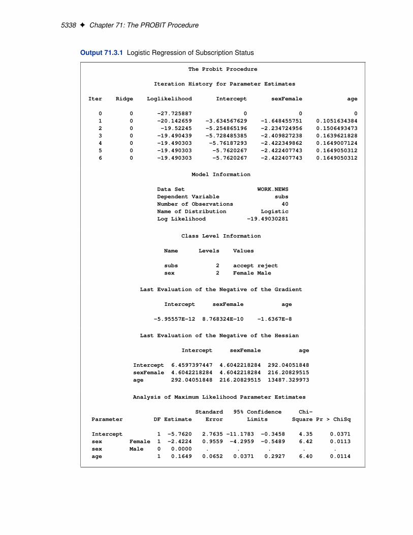
5338 F Chapter 71: The PROBIT Procedure
Output 71.3.1 Logistic Regression of Subscription Status
The Probit Procedure
Iteration History for Parameter Estimates
Iter Ridge Loglikelihood Intercept sexFemale age
0 0 -27.725887 0 0 01 0 -20.142659 -3.634567629 -1.648455751 0.10516343842 0 -19.52245 -5.254865196 -2.234724956 0.15064934733 0 -19.490439 -5.728485385 -2.409827238 0.16396218284 0 -19.490303 -5.76187293 -2.422349862 0.16490071245 0 -19.490303 -5.7620267 -2.422407743 0.16490503126 0 -19.490303 -5.7620267 -2.422407743 0.1649050312
Model Information
Data Set WORK.NEWSDependent Variable subsNumber of Observations 40Name of Distribution LogisticLog Likelihood -19.49030281
Class Level Information
Name Levels Values
subs 2 accept rejectsex 2 Female Male
Last Evaluation of the Negative of the Gradient
Intercept sexFemale age
-5.95557E-12 8.768324E-10 -1.6367E-8
Last Evaluation of the Negative of the Hessian
Intercept sexFemale age
Intercept 6.4597397447 4.6042218284 292.04051848sexFemale 4.6042218284 4.6042218284 216.20829515age 292.04051848 216.20829515 13487.329973
Analysis of Maximum Likelihood Parameter Estimates
Standard 95% Confidence Chi-Parameter DF Estimate Error Limits Square Pr > ChiSq
Intercept 1 -5.7620 2.7635 -11.1783 -0.3458 4.35 0.0371sex Female 1 -2.4224 0.9559 -4.2959 -0.5489 6.42 0.0113sex Male 0 0.0000 . . . . .age 1 0.1649 0.0652 0.0371 0.2927 6.40 0.0114
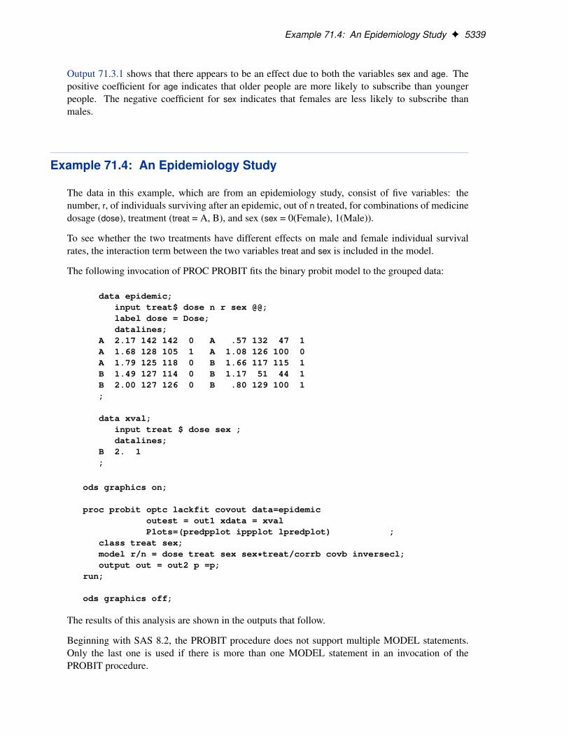
Example 71.4: An Epidemiology Study F 5339
Output 71.3.1 shows that there appears to be an effect due to both the variables sex and age. Thepositive coefficient for age indicates that older people are more likely to subscribe than youngerpeople. The negative coefficient for sex indicates that females are less likely to subscribe thanmales.
Example 71.4: An Epidemiology Study
The data in this example, which are from an epidemiology study, consist of five variables: thenumber, r, of individuals surviving after an epidemic, out of n treated, for combinations of medicinedosage (dose), treatment (treat = A, B), and sex (sex = 0(Female), 1(Male)).
To see whether the two treatments have different effects on male and female individual survivalrates, the interaction term between the two variables treat and sex is included in the model.
The following invocation of PROC PROBIT fits the binary probit model to the grouped data:
data epidemic;input treat$ dose n r sex @@;label dose = Dose;datalines;
A 2.17 142 142 0 A .57 132 47 1A 1.68 128 105 1 A 1.08 126 100 0A 1.79 125 118 0 B 1.66 117 115 1B 1.49 127 114 0 B 1.17 51 44 1B 2.00 127 126 0 B .80 129 100 1;
data xval;input treat $ dose sex ;datalines;
B 2. 1;
ods graphics on;
proc probit optc lackfit covout data=epidemicoutest = out1 xdata = xvalPlots=(predpplot ippplot lpredplot) ;
class treat sex;model r/n = dose treat sex sex*treat/corrb covb inversecl;output out = out2 p =p;
run;
ods graphics off;
The results of this analysis are shown in the outputs that follow.
Beginning with SAS 8.2, the PROBIT procedure does not support multiple MODEL statements.Only the last one is used if there is more than one MODEL statement in an invocation of thePROBIT procedure.
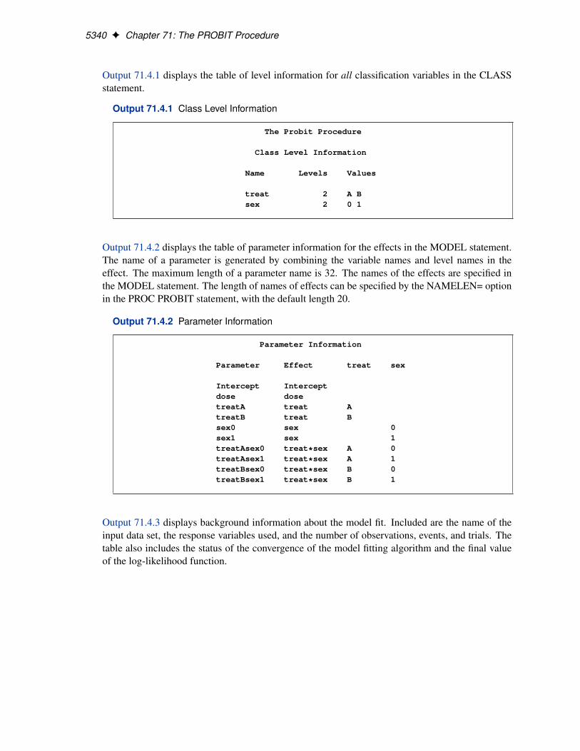
5340 F Chapter 71: The PROBIT Procedure
Output 71.4.1 displays the table of level information for all classification variables in the CLASSstatement.
Output 71.4.1 Class Level Information
The Probit Procedure
Class Level Information
Name Levels Values
treat 2 A Bsex 2 0 1
Output 71.4.2 displays the table of parameter information for the effects in the MODEL statement.The name of a parameter is generated by combining the variable names and level names in theeffect. The maximum length of a parameter name is 32. The names of the effects are specified inthe MODEL statement. The length of names of effects can be specified by the NAMELEN= optionin the PROC PROBIT statement, with the default length 20.
Output 71.4.2 Parameter Information
Parameter Information
Parameter Effect treat sex
Intercept Interceptdose dosetreatA treat AtreatB treat Bsex0 sex 0sex1 sex 1treatAsex0 treat*sex A 0treatAsex1 treat*sex A 1treatBsex0 treat*sex B 0treatBsex1 treat*sex B 1
Output 71.4.3 displays background information about the model fit. Included are the name of theinput data set, the response variables used, and the number of observations, events, and trials. Thetable also includes the status of the convergence of the model fitting algorithm and the final valueof the log-likelihood function.
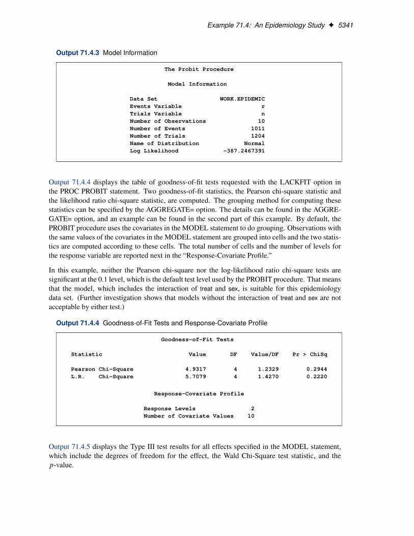
Example 71.4: An Epidemiology Study F 5341
Output 71.4.3 Model Information
The Probit Procedure
Model Information
Data Set WORK.EPIDEMICEvents Variable rTrials Variable nNumber of Observations 10Number of Events 1011Number of Trials 1204Name of Distribution NormalLog Likelihood -387.2467391
Output 71.4.4 displays the table of goodness-of-fit tests requested with the LACKFIT option inthe PROC PROBIT statement. Two goodness-of-fit statistics, the Pearson chi-square statistic andthe likelihood ratio chi-square statistic, are computed. The grouping method for computing thesestatistics can be specified by the AGGREGATE= option. The details can be found in the AGGRE-GATE= option, and an example can be found in the second part of this example. By default, thePROBIT procedure uses the covariates in the MODEL statement to do grouping. Observations withthe same values of the covariates in the MODEL statement are grouped into cells and the two statis-tics are computed according to these cells. The total number of cells and the number of levels forthe response variable are reported next in the “Response-Covariate Profile.”
In this example, neither the Pearson chi-square nor the log-likelihood ratio chi-square tests aresignificant at the 0.1 level, which is the default test level used by the PROBIT procedure. That meansthat the model, which includes the interaction of treat and sex, is suitable for this epidemiologydata set. (Further investigation shows that models without the interaction of treat and sex are notacceptable by either test.)
Output 71.4.4 Goodness-of-Fit Tests and Response-Covariate Profile
Goodness-of-Fit Tests
Statistic Value DF Value/DF Pr > ChiSq
Pearson Chi-Square 4.9317 4 1.2329 0.2944L.R. Chi-Square 5.7079 4 1.4270 0.2220
Response-Covariate Profile
Response Levels 2Number of Covariate Values 10
Output 71.4.5 displays the Type III test results for all effects specified in the MODEL statement,which include the degrees of freedom for the effect, the Wald Chi-Square test statistic, and thep-value.
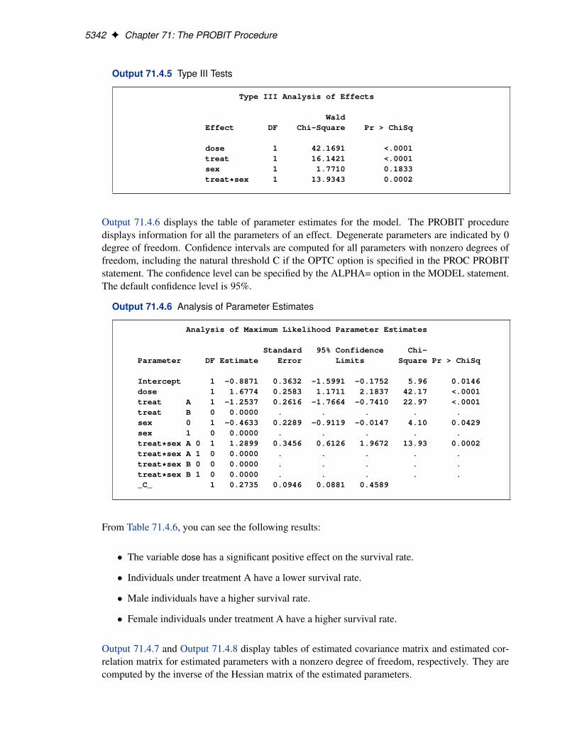
5342 F Chapter 71: The PROBIT Procedure
Output 71.4.5 Type III Tests
Type III Analysis of Effects
WaldEffect DF Chi-Square Pr > ChiSq
dose 1 42.1691 <.0001treat 1 16.1421 <.0001sex 1 1.7710 0.1833treat*sex 1 13.9343 0.0002
Output 71.4.6 displays the table of parameter estimates for the model. The PROBIT proceduredisplays information for all the parameters of an effect. Degenerate parameters are indicated by 0degree of freedom. Confidence intervals are computed for all parameters with nonzero degrees offreedom, including the natural threshold C if the OPTC option is specified in the PROC PROBITstatement. The confidence level can be specified by the ALPHA= option in the MODEL statement.The default confidence level is 95%.
Output 71.4.6 Analysis of Parameter Estimates
Analysis of Maximum Likelihood Parameter Estimates
Standard 95% Confidence Chi-Parameter DF Estimate Error Limits Square Pr > ChiSq
Intercept 1 -0.8871 0.3632 -1.5991 -0.1752 5.96 0.0146dose 1 1.6774 0.2583 1.1711 2.1837 42.17 <.0001treat A 1 -1.2537 0.2616 -1.7664 -0.7410 22.97 <.0001treat B 0 0.0000 . . . . .sex 0 1 -0.4633 0.2289 -0.9119 -0.0147 4.10 0.0429sex 1 0 0.0000 . . . . .treat*sex A 0 1 1.2899 0.3456 0.6126 1.9672 13.93 0.0002treat*sex A 1 0 0.0000 . . . . .treat*sex B 0 0 0.0000 . . . . .treat*sex B 1 0 0.0000 . . . . ._C_ 1 0.2735 0.0946 0.0881 0.4589
From Table 71.4.6, you can see the following results:
� The variable dose has a significant positive effect on the survival rate.
� Individuals under treatment A have a lower survival rate.
� Male individuals have a higher survival rate.
� Female individuals under treatment A have a higher survival rate.
Output 71.4.7 and Output 71.4.8 display tables of estimated covariance matrix and estimated cor-relation matrix for estimated parameters with a nonzero degree of freedom, respectively. They arecomputed by the inverse of the Hessian matrix of the estimated parameters.
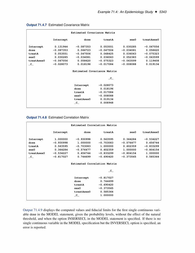
Example 71.4: An Epidemiology Study F 5343
Output 71.4.7 Estimated Covariance Matrix
Estimated Covariance Matrix
Intercept dose treatA sex0 treatAsex0
Intercept 0.131944 -0.087353 0.053551 0.030285 -0.067056dose -0.087353 0.066723 -0.047506 -0.034081 0.058620treatA 0.053551 -0.047506 0.068425 0.036063 -0.075323sex0 0.030285 -0.034081 0.036063 0.052383 -0.063599treatAsex0 -0.067056 0.058620 -0.075323 -0.063599 0.119408_C_ -0.028073 0.018196 -0.017084 -0.008088 0.019134
Estimated Covariance Matrix
_C_
Intercept -0.028073dose 0.018196treatA -0.017084sex0 -0.008088treatAsex0 0.019134_C_ 0.008948
Output 71.4.8 Estimated Correlation Matrix
Estimated Correlation Matrix
Intercept dose treatA sex0 treatAsex0
Intercept 1.000000 -0.930998 0.563595 0.364284 -0.534227dose -0.930998 1.000000 -0.703083 -0.576477 0.656744treatA 0.563595 -0.703083 1.000000 0.602359 -0.833299sex0 0.364284 -0.576477 0.602359 1.000000 -0.804154treatAsex0 -0.534227 0.656744 -0.833299 -0.804154 1.000000_C_ -0.817027 0.744699 -0.690420 -0.373565 0.585364
Estimated Correlation Matrix
_C_
Intercept -0.817027dose 0.744699treatA -0.690420sex0 -0.373565treatAsex0 0.585364_C_ 1.000000
Output 71.4.9 displays the computed values and fiducial limits for the first single continuous vari-able dose in the MODEL statement, given the probability levels, without the effect of the naturalthreshold, and when the option INSERSECL in the MODEL statement is specified. If there is nosingle continuous variable in the MODEL specification but the INVERSECL option is specified, anerror is reported.
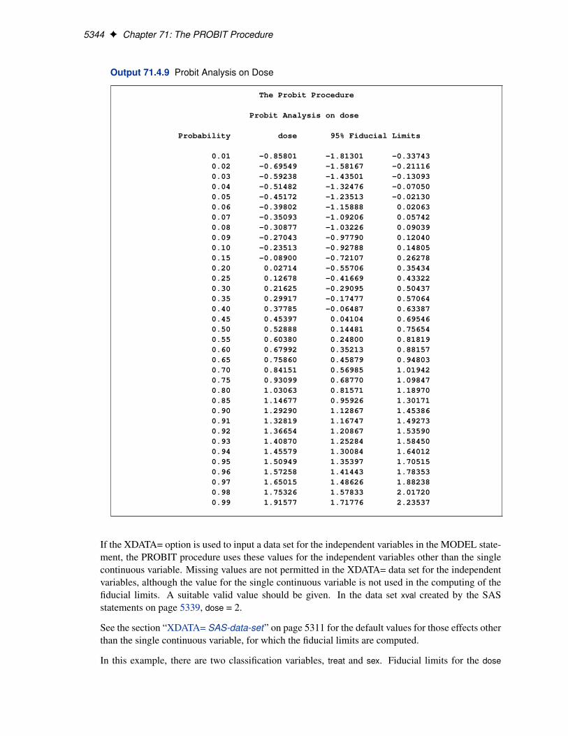
5344 F Chapter 71: The PROBIT Procedure
Output 71.4.9 Probit Analysis on Dose
The Probit Procedure
Probit Analysis on dose
Probability dose 95% Fiducial Limits
0.01 -0.85801 -1.81301 -0.337430.02 -0.69549 -1.58167 -0.211160.03 -0.59238 -1.43501 -0.130930.04 -0.51482 -1.32476 -0.070500.05 -0.45172 -1.23513 -0.021300.06 -0.39802 -1.15888 0.020630.07 -0.35093 -1.09206 0.057420.08 -0.30877 -1.03226 0.090390.09 -0.27043 -0.97790 0.120400.10 -0.23513 -0.92788 0.148050.15 -0.08900 -0.72107 0.262780.20 0.02714 -0.55706 0.354340.25 0.12678 -0.41669 0.433220.30 0.21625 -0.29095 0.504370.35 0.29917 -0.17477 0.570640.40 0.37785 -0.06487 0.633870.45 0.45397 0.04104 0.695460.50 0.52888 0.14481 0.756540.55 0.60380 0.24800 0.818190.60 0.67992 0.35213 0.881570.65 0.75860 0.45879 0.948030.70 0.84151 0.56985 1.019420.75 0.93099 0.68770 1.098470.80 1.03063 0.81571 1.189700.85 1.14677 0.95926 1.301710.90 1.29290 1.12867 1.453860.91 1.32819 1.16747 1.492730.92 1.36654 1.20867 1.535900.93 1.40870 1.25284 1.584500.94 1.45579 1.30084 1.640120.95 1.50949 1.35397 1.705150.96 1.57258 1.41443 1.783530.97 1.65015 1.48626 1.882380.98 1.75326 1.57833 2.017200.99 1.91577 1.71776 2.23537
If the XDATA= option is used to input a data set for the independent variables in the MODEL state-ment, the PROBIT procedure uses these values for the independent variables other than the singlecontinuous variable. Missing values are not permitted in the XDATA= data set for the independentvariables, although the value for the single continuous variable is not used in the computing of thefiducial limits. A suitable valid value should be given. In the data set xval created by the SASstatements on page 5339, dose = 2.
See the section “XDATA= SAS-data-set” on page 5311 for the default values for those effects otherthan the single continuous variable, for which the fiducial limits are computed.
In this example, there are two classification variables, treat and sex. Fiducial limits for the dose
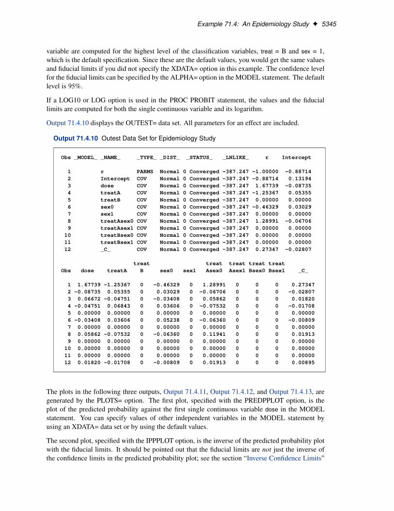
Example 71.4: An Epidemiology Study F 5345
variable are computed for the highest level of the classification variables, treat = B and sex = 1,which is the default specification. Since these are the default values, you would get the same valuesand fiducial limits if you did not specify the XDATA= option in this example. The confidence levelfor the fiducial limits can be specified by the ALPHA= option in the MODEL statement. The defaultlevel is 95%.
If a LOG10 or LOG option is used in the PROC PROBIT statement, the values and the fiduciallimits are computed for both the single continuous variable and its logarithm.
Output 71.4.10 displays the OUTEST= data set. All parameters for an effect are included.
Output 71.4.10 Outest Data Set for Epidemiology Study
Obs _MODEL_ _NAME_ _TYPE_ _DIST_ _STATUS_ _LNLIKE_ r Intercept
1 r PARMS Normal 0 Converged -387.247 -1.00000 -0.887142 Intercept COV Normal 0 Converged -387.247 -0.88714 0.131943 dose COV Normal 0 Converged -387.247 1.67739 -0.087354 treatA COV Normal 0 Converged -387.247 -1.25367 0.053555 treatB COV Normal 0 Converged -387.247 0.00000 0.000006 sex0 COV Normal 0 Converged -387.247 -0.46329 0.030297 sex1 COV Normal 0 Converged -387.247 0.00000 0.000008 treatAsex0 COV Normal 0 Converged -387.247 1.28991 -0.067069 treatAsex1 COV Normal 0 Converged -387.247 0.00000 0.00000
10 treatBsex0 COV Normal 0 Converged -387.247 0.00000 0.0000011 treatBsex1 COV Normal 0 Converged -387.247 0.00000 0.0000012 _C_ COV Normal 0 Converged -387.247 0.27347 -0.02807
treat treat treat treat treatObs dose treatA B sex0 sex1 Asex0 Asex1 Bsex0 Bsex1 _C_
1 1.67739 -1.25367 0 -0.46329 0 1.28991 0 0 0 0.273472 -0.08735 0.05355 0 0.03029 0 -0.06706 0 0 0 -0.028073 0.06672 -0.04751 0 -0.03408 0 0.05862 0 0 0 0.018204 -0.04751 0.06843 0 0.03606 0 -0.07532 0 0 0 -0.017085 0.00000 0.00000 0 0.00000 0 0.00000 0 0 0 0.000006 -0.03408 0.03606 0 0.05238 0 -0.06360 0 0 0 -0.008097 0.00000 0.00000 0 0.00000 0 0.00000 0 0 0 0.000008 0.05862 -0.07532 0 -0.06360 0 0.11941 0 0 0 0.019139 0.00000 0.00000 0 0.00000 0 0.00000 0 0 0 0.00000
10 0.00000 0.00000 0 0.00000 0 0.00000 0 0 0 0.0000011 0.00000 0.00000 0 0.00000 0 0.00000 0 0 0 0.0000012 0.01820 -0.01708 0 -0.00809 0 0.01913 0 0 0 0.00895
The plots in the following three outputs, Output 71.4.11, Output 71.4.12, and Output 71.4.13, aregenerated by the PLOTS= option. The first plot, specified with the PREDPPLOT option, is theplot of the predicted probability against the first single continuous variable dose in the MODELstatement. You can specify values of other independent variables in the MODEL statement byusing an XDATA= data set or by using the default values.
The second plot, specified with the IPPPLOT option, is the inverse of the predicted probability plotwith the fiducial limits. It should be pointed out that the fiducial limits are not just the inverse ofthe confidence limits in the predicted probability plot; see the section “Inverse Confidence Limits”
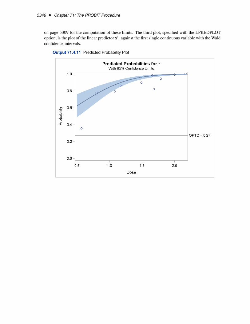
5346 F Chapter 71: The PROBIT Procedure
on page 5309 for the computation of these limits. The third plot, specified with the LPREDPLOToption, is the plot of the linear predictor x0˛ against the first single continuous variable with the Waldconfidence intervals.
Output 71.4.11 Predicted Probability Plot
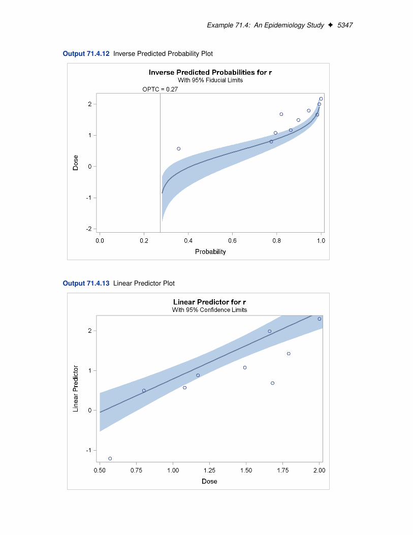
Example 71.4: An Epidemiology Study F 5347
Output 71.4.12 Inverse Predicted Probability Plot
Output 71.4.13 Linear Predictor Plot
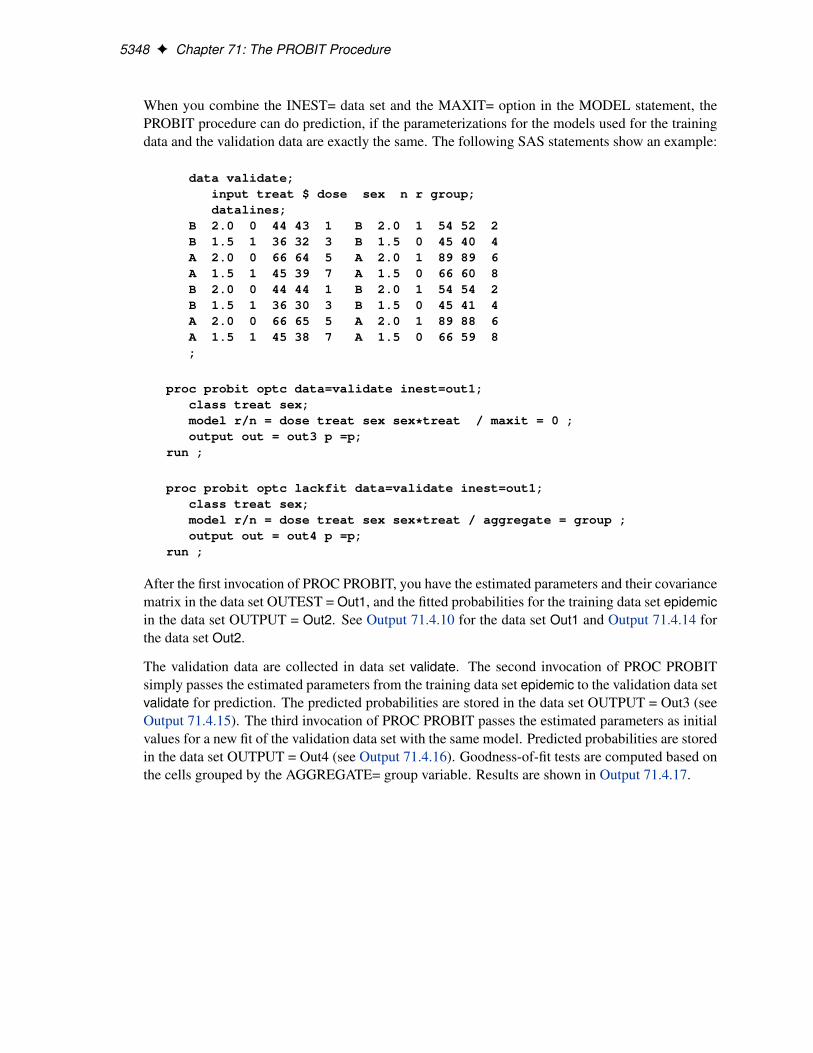
5348 F Chapter 71: The PROBIT Procedure
When you combine the INEST= data set and the MAXIT= option in the MODEL statement, thePROBIT procedure can do prediction, if the parameterizations for the models used for the trainingdata and the validation data are exactly the same. The following SAS statements show an example:
data validate;input treat $ dose sex n r group;datalines;
B 2.0 0 44 43 1 B 2.0 1 54 52 2B 1.5 1 36 32 3 B 1.5 0 45 40 4A 2.0 0 66 64 5 A 2.0 1 89 89 6A 1.5 1 45 39 7 A 1.5 0 66 60 8B 2.0 0 44 44 1 B 2.0 1 54 54 2B 1.5 1 36 30 3 B 1.5 0 45 41 4A 2.0 0 66 65 5 A 2.0 1 89 88 6A 1.5 1 45 38 7 A 1.5 0 66 59 8;
proc probit optc data=validate inest=out1;class treat sex;model r/n = dose treat sex sex*treat / maxit = 0 ;output out = out3 p =p;
run ;
proc probit optc lackfit data=validate inest=out1;class treat sex;model r/n = dose treat sex sex*treat / aggregate = group ;output out = out4 p =p;
run ;
After the first invocation of PROC PROBIT, you have the estimated parameters and their covariancematrix in the data set OUTEST = Out1, and the fitted probabilities for the training data set epidemicin the data set OUTPUT = Out2. See Output 71.4.10 for the data set Out1 and Output 71.4.14 forthe data set Out2.
The validation data are collected in data set validate. The second invocation of PROC PROBITsimply passes the estimated parameters from the training data set epidemic to the validation data setvalidate for prediction. The predicted probabilities are stored in the data set OUTPUT = Out3 (seeOutput 71.4.15). The third invocation of PROC PROBIT passes the estimated parameters as initialvalues for a new fit of the validation data set with the same model. Predicted probabilities are storedin the data set OUTPUT = Out4 (see Output 71.4.16). Goodness-of-fit tests are computed based onthe cells grouped by the AGGREGATE= group variable. Results are shown in Output 71.4.17.
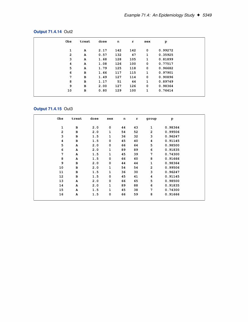
Example 71.4: An Epidemiology Study F 5349
Output 71.4.14 Out2
Obs treat dose n r sex p
1 A 2.17 142 142 0 0.992722 A 0.57 132 47 1 0.359253 A 1.68 128 105 1 0.818994 A 1.08 126 100 0 0.775175 A 1.79 125 118 0 0.966826 B 1.66 117 115 1 0.979017 B 1.49 127 114 0 0.908968 B 1.17 51 44 1 0.897499 B 2.00 127 126 0 0.98364
10 B 0.80 129 100 1 0.76414
Output 71.4.15 Out3
Obs treat dose sex n r group p
1 B 2.0 0 44 43 1 0.983642 B 2.0 1 54 52 2 0.995063 B 1.5 1 36 32 3 0.962474 B 1.5 0 45 40 4 0.911455 A 2.0 0 66 64 5 0.985006 A 2.0 1 89 89 6 0.918357 A 1.5 1 45 39 7 0.743008 A 1.5 0 66 60 8 0.916669 B 2.0 0 44 44 1 0.98364
10 B 2.0 1 54 54 2 0.9950611 B 1.5 1 36 30 3 0.9624712 B 1.5 0 45 41 4 0.9114513 A 2.0 0 66 65 5 0.9850014 A 2.0 1 89 88 6 0.9183515 A 1.5 1 45 38 7 0.7430016 A 1.5 0 66 59 8 0.91666
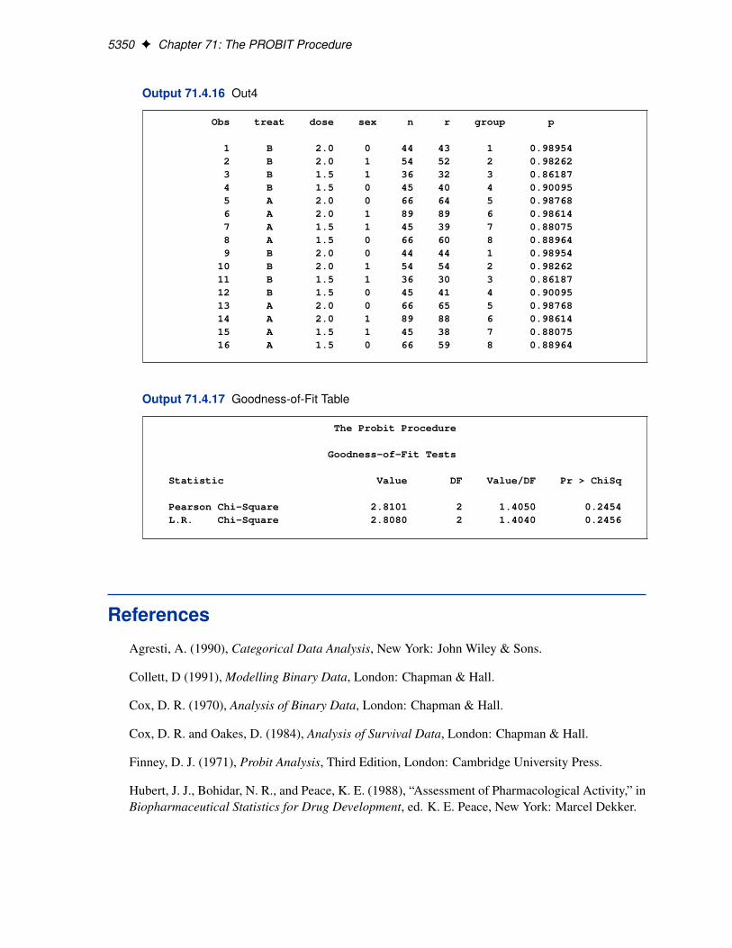
5350 F Chapter 71: The PROBIT Procedure
Output 71.4.16 Out4
Obs treat dose sex n r group p
1 B 2.0 0 44 43 1 0.989542 B 2.0 1 54 52 2 0.982623 B 1.5 1 36 32 3 0.861874 B 1.5 0 45 40 4 0.900955 A 2.0 0 66 64 5 0.987686 A 2.0 1 89 89 6 0.986147 A 1.5 1 45 39 7 0.880758 A 1.5 0 66 60 8 0.889649 B 2.0 0 44 44 1 0.98954
10 B 2.0 1 54 54 2 0.9826211 B 1.5 1 36 30 3 0.8618712 B 1.5 0 45 41 4 0.9009513 A 2.0 0 66 65 5 0.9876814 A 2.0 1 89 88 6 0.9861415 A 1.5 1 45 38 7 0.8807516 A 1.5 0 66 59 8 0.88964
Output 71.4.17 Goodness-of-Fit Table
The Probit Procedure
Goodness-of-Fit Tests
Statistic Value DF Value/DF Pr > ChiSq
Pearson Chi-Square 2.8101 2 1.4050 0.2454L.R. Chi-Square 2.8080 2 1.4040 0.2456
References
Agresti, A. (1990), Categorical Data Analysis, New York: John Wiley & Sons.
Collett, D (1991), Modelling Binary Data, London: Chapman & Hall.
Cox, D. R. (1970), Analysis of Binary Data, London: Chapman & Hall.
Cox, D. R. and Oakes, D. (1984), Analysis of Survival Data, London: Chapman & Hall.
Finney, D. J. (1971), Probit Analysis, Third Edition, London: Cambridge University Press.
Hubert, J. J., Bohidar, N. R., and Peace, K. E. (1988), “Assessment of Pharmacological Activity,” inBiopharmaceutical Statistics for Drug Development, ed. K. E. Peace, New York: Marcel Dekker.
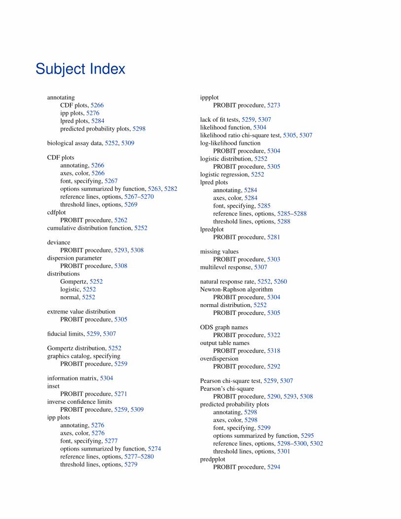
Subject Index
annotatingCDF plots, 5266ipp plots, 5276lpred plots, 5284predicted probability plots, 5298
biological assay data, 5252, 5309
CDF plotsannotating, 5266axes, color, 5266font, specifying, 5267options summarized by function, 5263, 5282reference lines, options, 5267–5270threshold lines, options, 5269
cdfplotPROBIT procedure, 5262
cumulative distribution function, 5252
deviancePROBIT procedure, 5293, 5308
dispersion parameterPROBIT procedure, 5308
distributionsGompertz, 5252logistic, 5252normal, 5252
extreme value distributionPROBIT procedure, 5305
fiducial limits, 5259, 5307
Gompertz distribution, 5252graphics catalog, specifying
PROBIT procedure, 5259
information matrix, 5304inset
PROBIT procedure, 5271inverse confidence limits
PROBIT procedure, 5259, 5309ipp plots
annotating, 5276axes, color, 5276font, specifying, 5277options summarized by function, 5274reference lines, options, 5277–5280threshold lines, options, 5279
ippplotPROBIT procedure, 5273
lack of fit tests, 5259, 5307likelihood function, 5304likelihood ratio chi-square test, 5305, 5307log-likelihood function
PROBIT procedure, 5304logistic distribution, 5252
PROBIT procedure, 5305logistic regression, 5252lpred plots
annotating, 5284axes, color, 5284font, specifying, 5285reference lines, options, 5285–5288threshold lines, options, 5288
lpredplotPROBIT procedure, 5281
missing valuesPROBIT procedure, 5303
multilevel response, 5307
natural response rate, 5252, 5260Newton-Raphson algorithm
PROBIT procedure, 5304normal distribution, 5252
PROBIT procedure, 5305
ODS graph namesPROBIT procedure, 5322
output table namesPROBIT procedure, 5318
overdispersionPROBIT procedure, 5292
Pearson chi-square test, 5259, 5307Pearson’s chi-square
PROBIT procedure, 5290, 5293, 5308predicted probability plots
annotating, 5298axes, color, 5298font, specifying, 5299options summarized by function, 5295reference lines, options, 5298–5300, 5302threshold lines, options, 5301
predpplotPROBIT procedure, 5294
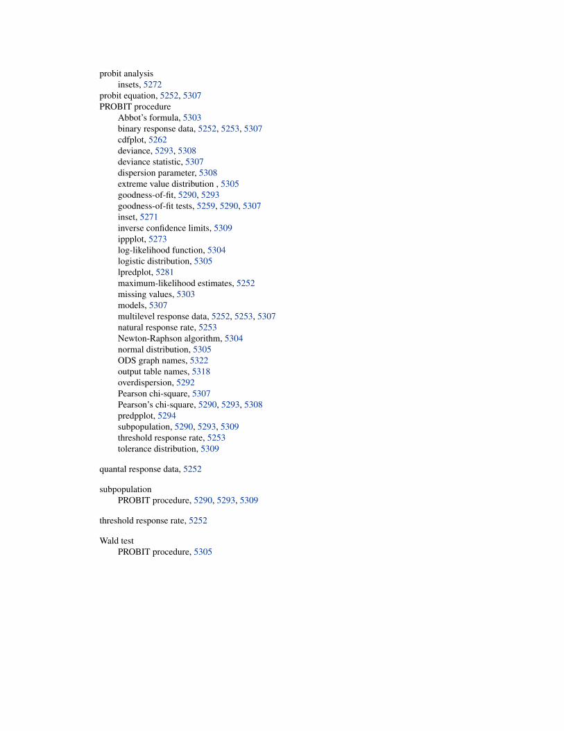
probit analysisinsets, 5272
probit equation, 5252, 5307PROBIT procedure
Abbot’s formula, 5303binary response data, 5252, 5253, 5307cdfplot, 5262deviance, 5293, 5308deviance statistic, 5307dispersion parameter, 5308extreme value distribution , 5305goodness-of-fit, 5290, 5293goodness-of-fit tests, 5259, 5290, 5307inset, 5271inverse confidence limits, 5309ippplot, 5273log-likelihood function, 5304logistic distribution, 5305lpredplot, 5281maximum-likelihood estimates, 5252missing values, 5303models, 5307multilevel response data, 5252, 5253, 5307natural response rate, 5253Newton-Raphson algorithm, 5304normal distribution, 5305ODS graph names, 5322output table names, 5318overdispersion, 5292Pearson chi-square, 5307Pearson’s chi-square, 5290, 5293, 5308predpplot, 5294subpopulation, 5290, 5293, 5309threshold response rate, 5253tolerance distribution, 5309
quantal response data, 5252
subpopulationPROBIT procedure, 5290, 5293, 5309
threshold response rate, 5252
Wald testPROBIT procedure, 5305
Syntax Index
AGGREGATE= optionMODEL statement (PROBIT), 5290
CDFPLOT statement, see PROBIT procedure,CDFPLOT statement, see PROBITprocedure, CDFPLOT statement
options summarized by function, 5263PROBIT procedure, 5262
COVOUT optionPROC PROBIT statement, 5258
DATA= optionPROC PROBIT statement, 5258
GOUT= optionPROC PROBIT statement, 5259
HPROB= optionPROC PROBIT statement, 5259
INEST= optionPROC PROBIT statement, 5259
INSET statementPROBIT procedure, 5271
INVERSECL optionPROC PROBIT statement, 5259
IPPPLOT statementoptions summarized by function, 5274PROBIT procedure, 5273
LACKFIT optionPROC PROBIT statement, 5259
LOG optionPROC PROBIT statement, 5259
LOG10 optionPROC PROBIT statement, 5260
LPREDPLOT statementoptions summarized by function, 5282PROBIT procedure, 5281
NAMELEN= optionPROC PROBIT statement, 5260
NOPRINT optionPROC PROBIT statement, 5260
OPTC optionPROC PROBIT statement, 5258, 5260
optionsCDFPLOT statement (PROBIT), 5263IPPPLOT statement (PROBIT), 5274
LPREDPLOT statement (PROBIT), 5281PREDPPLOT statement (PROBIT), 5295
ORDER= optionPROC PROBIT statement, 5260
OUTEST= optionPROC PROBIT statement, 5260
PLOT= optionPROC PROBIT statement, 5261
PREDPPLOT statementoptions summarized by function, 5295PROBIT procedure, 5294
PROBIT, 5252PROBIT procedure, 5252
syntax, 5257PROBIT procedure, BY statement, 5262PROBIT procedure, CDFPLOT statement, 5262
ANNOTATE= option, 5266CAXIS= option, 5266CFIT= option, 5266CFRAME= option, 5266CGRID= option, 5266CHREF= option, 5267CLABBOX= option, 5266CTEXT= option, 5267CVREF= option, 5267DESCRIPTION= option, 5267FONT= option, 5267HAXIS= option, 5267HEIGHT= option, 5267HLOWER= option, 5267HOFFSET= option, 5267HREF= option, 5268HREFLABELS= option, 5268HREFLABPOS= option, 5268HUPPER= option, 5268INBORDER option, 5268LEVEL option, 5268LFIT option, 5268LGRID option, 5268LHREF= option, 5268LVREF= option, 5269NAME= option, 5269NOFIT option, 5269NOFRAME option, 5269NOGRID option, 5269NOHLABEL option, 5269NOHTICK option, 5269
NOTHRESH option, 5269NOVLABEL option, 5269NOVTICK option, 5269options, 5263THRESHLABPOS= option, 5269VAR= option, 5263VAXIS= option, 5269VAXISLABEL= option, 5270VLOWER= option, 5270VREF= option, 5270VREFLABELS= option, 5270VREFLABPOS= option, 5270VUPPER= option, 5270WAXIS= option, 5270WFIT= option, 5270WGRID= option, 5270WREFL= option, 5270
PROBIT procedure, CLASS statement, 5271PROBIT procedure, INSET statement, 5271,
5272keywords, 5272
PROBIT procedure, IPPPLOT statement, 5273ANNOTATE= option, 5276CAXIS= option, 5276CFIT= option, 5277CFRAME= option, 5277CGRID= option, 5277CHREF= option, 5277CTEXT= option, 5277CVREF= option, 5277DESCRIPTION= option, 5277FONT= option, 5277HAXIS= option, 5277HEIGHT= option, 5277HLOWER= option, 5278HOFFSET= option, 5278HREF= option, 5278HREFLABELS= option, 5278HREFLABPOS= option, 5278HUPPER= option, 5278INBORDER option, 5278LFIT option, 5278LGRID option, 5278LHREF= option, 5279LVREF= option, 5279NAME= option, 5279NOCONF option, 5279NODATA option, 5279NOFIT option, 5279NOFRAME option, 5279NOGRID option, 5279NOHLABEL option, 5279NOHTICK option, 5279NOTHRESH option, 5279
NOVLABEL option, 5279NOVTICK option, 5279options, 5274THRESHLABPOS= option, 5279VAR= option, 5273VAXIS= option, 5280VAXISLABEL= option, 5280VLOWER= option, 5280VREF= option, 5280VREFLABELS= option, 5280VREFLABPOS= option, 5280VUPPER= option, 5280WAXIS= option, 5280WFIT= option, 5281WGRID= option, 5281WREFL= option, 5281
PROBIT procedure, LPREDPLOT statement,5281
ANNOTATE= option, 5284CAXIS= option, 5284CFIT= option, 5284CFRAME= option, 5285CGRID= option, 5285CHREF= option, 5285CTEXT= option, 5285CVREF= option, 5285DESCRIPTION= option, 5285FONT= option, 5285HAXIS= option, 5285HEIGHT= option, 5285HLOWER= option, 5286HOFFSET= option, 5286HREF= option, 5286HREFLABELS= option, 5286HREFLABPOS= option, 5286HUPPER= option, 5286INBORDER option, 5286LEVEL option, 5286LFIT option, 5287LGRID option, 5287LHREF= option, 5287LVREF= option, 5287NAME= option, 5287NOCONF option, 5287NODATA option, 5287NOFIT option, 5287NOFRAME option, 5287NOGRID option, 5287NOHLABEL option, 5287NOHTICK option, 5287NOTHRESH option, 5287NOVLABEL option, 5287NOVTICK option, 5288options, 5281
THRESHLABPOS= option, 5288VAR= option, 5281VAXIS= option, 5288VAXISLABEL= option, 5288VLOWER= option, 5288VREF= option, 5288VREFLABELS= option, 5288VREFLABPOS= option, 5288VUPPER= option, 5289WAXIS= option, 5289WFIT= option, 5289WGRID= option, 5289WREFL= option, 5289
PROBIT procedure, MODEL statement, 5289AGGREGATE= option, 5290ALPHA= option, 5290CONVERGE option, 5290CORRB option, 5290COVB option, 5290DISTRIBUTION= option, 5291HPROB= option, 5291INITIAL option, 5291INTERCEPT= option, 5291INVERSECL option, 5291ITPRINT option, 5292MAXITER= option, 5292NOINT option, 5292SCALE= option, 5292SINGULAR= option, 5293
PROBIT procedure, OUTPUT statement, 5293PROBIT procedure, PREDPLOT statement
LEVEL option, 5300PROBIT procedure, PREDPPLOT statement,
5294ANNOTATE= option, 5298CAXIS= option, 5298CFIT= option, 5298CFRAME= option, 5298CGRID= option, 5298CHREF= option, 5298CTEXT= option, 5299CVREF= option, 5299DESCRIPTION= option, 5299FONT= option, 5299HAXIS= option, 5299HEIGHT= option, 5299HLOWER= option, 5299HOFFSET= option, 5299HREF= option, 5299HREFLABELS= option, 5300HREFLABPOS= option, 5300HUPPER= option, 5299INBORDER option, 5300LFIT option, 5300
LGRID option, 5300LHREF= option, 5300LVREF= option, 5300NAME= option, 5301NOCONF option, 5301NODATA option, 5301NOFIT option, 5301NOFRAME option, 5301NOGRID option, 5301NOHLABEL option, 5301NOHTICK option, 5301NOTHRESH option, 5301NOVLABEL option, 5301NOVTICK option, 5301options, 5295THRESHLABPOS= option, 5301VAR= option, 5294VAXIS= option, 5301VAXISLABEL= option, 5302VLOWER= option, 5302VREF= option, 5302VREFLABELS= option, 5302VREFLABPOS= option, 5302VUPPER= option, 5302WAXIS= option, 5302WFIT= option, 5302WGRID= option, 5302WREFL= option, 5302
PROBIT procedure, PROC PROBIT statement,5258
COVOUT option, 5258DATA= option, 5258GOUT= option, 5259HPROB= option, 5259INEST= option, 5259INVERSECL option, 5259LACKFIT option, 5259LOG option, 5259LOG10 option, 5260NAMELEN= option, 5260NOPRINT option, 5260OPTC option, 5258, 5260ORDER=option, 5260OUTEST= option, 5260PLOT= option, 5261XDATA= option, 5262
PROBIT procedure, WEIGHT statement, 5303PROC PROBIT statement, see PROBIT
procedure
SCALE= optionMODEL statement (PROBIT), 5292
VAR= option

CDFPLOT statement (PROBIT), 5263IPPPLOT statement (PROBIT), 5273LPREDPLOT statement (PROBIT), 5281PREDPPLOT statement (PROBIT), 5294
XDATA= optionPROC PROBIT statement, 5262
Your Turn
We welcome your feedback.
� If you have comments about this book, please send them [email protected]. Include the full title and page numbers (ifapplicable).
� If you have comments about the software, please send them [email protected].


SAS® Publishing Delivers!Whether you are new to the work force or an experienced professional, you need to distinguish yourself in this rapidly changing and competitive job market. SAS® Publishing provides you with a wide range of resources to help you set yourself apart. Visit us online at support.sas.com/bookstore.
SAS® Press Need to learn the basics? Struggling with a programming problem? You’ll find the expert answers that you need in example-rich books from SAS Press. Written by experienced SAS professionals from around the world, SAS Press books deliver real-world insights on a broad range of topics for all skill levels.
s u p p o r t . s a s . c o m / s a s p r e s sSAS® Documentation To successfully implement applications using SAS software, companies in every industry and on every continent all turn to the one source for accurate, timely, and reliable information: SAS documentation. We currently produce the following types of reference documentation to improve your work experience:
• Onlinehelpthatisbuiltintothesoftware.• Tutorialsthatareintegratedintotheproduct.• ReferencedocumentationdeliveredinHTMLandPDF– free on the Web. • Hard-copybooks.
s u p p o r t . s a s . c o m / p u b l i s h i n gSAS® Publishing News Subscribe to SAS Publishing News to receive up-to-date information about all new SAS titles, author podcasts, and new Web site features via e-mail. Complete instructions on how to subscribe, as well as access to past issues, are available at our Web site.
s u p p o r t . s a s . c o m / s p n
SAS and all other SAS Institute Inc. product or service names are registered trademarks or trademarks of SAS Institute Inc. in the USA and other countries. ® indicates USA registration. Otherbrandandproductnamesaretrademarksoftheirrespectivecompanies.©2009SASInstituteInc.Allrightsreserved.518177_1US.0109