SAS/STAT 9.2 User's Guide: The VARCLUS …...® 9.2 User’s Guide The VARCLUS Procedure (Book Excerpt) SAS ® Documentation This document is an individual chapter from SAS/STAT®

SAS/STAT® 9.2 User’s GuideThe VARCLUS Procedure(Book Excerpt)

SAS® Documentation

This document is an individual chapter from SAS/STAT® 9.2 User’s Guide.

The correct bibliographic citation for the complete manual is as follows: SAS Institute Inc. 2008. SAS/STAT® 9.2User’s Guide. Cary, NC: SAS Institute Inc.

Copyright © 2008, SAS Institute Inc., Cary, NC, USA

All rights reserved. Produced in the United States of America.

For a Web download or e-book: Your use of this publication shall be governed by the terms established by the vendorat the time you acquire this publication.

U.S. Government Restricted Rights Notice: Use, duplication, or disclosure of this software and related documentationby the U.S. government is subject to the Agreement with SAS Institute and the restrictions set forth in FAR 52.227-19,Commercial Computer Software-Restricted Rights (June 1987).

SAS Institute Inc., SAS Campus Drive, Cary, North Carolina 27513.

1st electronic book, March 20082nd electronic book, February 2009SAS® Publishing provides a complete selection of books and electronic products to help customers use SAS software toits fullest potential. For more information about our e-books, e-learning products, CDs, and hard-copy books, visit theSAS Publishing Web site at support.sas.com/publishing or call 1-800-727-3228.

SAS® and all other SAS Institute Inc. product or service names are registered trademarks or trademarks of SAS InstituteInc. in the USA and other countries. ® indicates USA registration.

Other brand and product names are registered trademarks or trademarks of their respective companies.

Chapter 93

The VARCLUS Procedure

ContentsOverview: VARCLUS Procedure . . . . . . . . . . . . . . . . . . . . . . . . . . . 7453Getting Started: VARCLUS Procedure . . . . . . . . . . . . . . . . . . . . . . . . 7455Syntax: VARCLUS Procedure . . . . . . . . . . . . . . . . . . . . . . . . . . . . 7460

PROC VARCLUS Statement . . . . . . . . . . . . . . . . . . . . . . . . . 7460BY Statement . . . . . . . . . . . . . . . . . . . . . . . . . . . . . . . . . 7466FREQ Statement . . . . . . . . . . . . . . . . . . . . . . . . . . . . . . . . 7466PARTIAL Statement . . . . . . . . . . . . . . . . . . . . . . . . . . . . . . 7467SEED Statement . . . . . . . . . . . . . . . . . . . . . . . . . . . . . . . . 7467VAR Statement . . . . . . . . . . . . . . . . . . . . . . . . . . . . . . . . . 7467WEIGHT Statement . . . . . . . . . . . . . . . . . . . . . . . . . . . . . . 7467

Details: VARCLUS Procedure . . . . . . . . . . . . . . . . . . . . . . . . . . . . 7468Missing Values . . . . . . . . . . . . . . . . . . . . . . . . . . . . . . . . . 7468Using the VARCLUS procedure . . . . . . . . . . . . . . . . . . . . . . . . 7468Output Data Sets . . . . . . . . . . . . . . . . . . . . . . . . . . . . . . . . 7469Computational Resources . . . . . . . . . . . . . . . . . . . . . . . . . . . 7471Interpreting VARCLUS Procedure Output . . . . . . . . . . . . . . . . . . . 7471Displayed Output . . . . . . . . . . . . . . . . . . . . . . . . . . . . . . . . 7472ODS Table Names . . . . . . . . . . . . . . . . . . . . . . . . . . . . . . . 7473

Example: VARCLUS Procedure . . . . . . . . . . . . . . . . . . . . . . . . . . . 7475Example 93.1: Correlations among Physical Variables . . . . . . . . . . . . 7475

References . . . . . . . . . . . . . . . . . . . . . . . . . . . . . . . . . . . . . . 7484

Overview: VARCLUS Procedure

The VARCLUS procedure divides a set of numeric variables into disjoint or hierarchical clusters.Associated with each cluster is a linear combination of the variables in the cluster. This linear com-bination can be either the first principal component (the default) or the centroid component (if youspecify the CENTROID option). The first principal component is a weighted average of the vari-ables that explains as much variance as possible. See Chapter 69, “The PRINCOMP Procedure,”for further details. Centroid components are unweighted averages of either the standardized vari-ables (the default) or the raw variables (if you specify the COVARIANCE option). The VARCLUS

7454 F Chapter 93: The VARCLUS Procedure

procedure tries to maximize the variance that is explained by the cluster components, summed overall the clusters.

The cluster components are oblique, not orthogonal, even when the cluster components are firstprincipal components. In an ordinary principal component analysis, all components are computedfrom the same variables, and the first principal component is orthogonal to the second principalcomponent and to every other principal component. In the VARCLUS procedure, each clustercomponent is computed from a different set of variables than all the other cluster components. Thefirst principal component of one cluster might be correlated with the first principal component ofanother cluster. Hence, the VARCLUS algorithm is a type of oblique component analysis.

As in principal component analysis, either the correlation or the covariance matrix can be analyzed.If correlations are used, all variables are treated as equally important. If covariances are used,variables with larger variances have more importance in the analysis.

The VARCLUS procedure creates an output data set that can be used with the SCORE procedureto compute component scores for each cluster. A second output data set can be used by the TREEprocedure to draw a tree diagram of hierarchical clusters.

The VARCLUS procedure can be used as a variable-reduction method. A large set of variables canoften be replaced by the set of cluster components with little loss of information. A given numberof cluster components does not generally explain as much variance as the same number of principalcomponents on the full set of variables, but the cluster components are usually easier to interpretthan the principal components, even if the latter are rotated.

For example, an educational test might contain 50 items. The VARCLUS procedure can be used todivide the items into, say, five clusters. Each cluster can then be treated as a subtest, with the subtestscores given by the cluster components. If the cluster components are centroid components of thecovariance matrix, each subtest score is simply the sum of the item scores for that cluster.

The VARCLUS algorithm is both divisive and iterative. By default, the VARCLUS procedurebegins with all variables in a single cluster. It then repeats the following steps:

1. A cluster is chosen for splitting. Depending on the options specified, the selected cluster haseither the smallest percentage of variation explained by its cluster component (using the PRO-PORTION= option) or the largest eigenvalue associated with the second principal component(using the MAXEIGEN= option).

2. The chosen cluster is split into two clusters by finding the first two principal components,performing an orthoblique rotation (raw quartimax rotation on the eigenvectors; Harris andKaiser 1964), and assigning each variable to the rotated component with which it has thehigher squared correlation.

3. Variables are iteratively reassigned to clusters to try to maximize the variance accountedfor by the cluster components. You can require the reassignment algorithms to maintain ahierarchical structure for the clusters.

Getting Started: VARCLUS Procedure F 7455

The procedure stops splitting when either of the following conditions holds:

� The number of clusters is greater than or equal to the maximum number of clusters as speci-fied by the MAXCLUSTERS= option is reached.

� Every cluster satisfies the stopping criteria specified by the PROPORTION= (percentage ofvariation explained) and/or the MAXEIGEN= (second eigenvalue) options.

By default, VARCLUS stops splitting when every cluster has only one eigenvalue greater than one,thus satisfying the most popular criterion for determining the sufficiency of a single underlyingdimension.

The iterative reassignment of variables to clusters proceeds in two phases. The first is a nearestcomponent sorting (NCS) phase, similar in principle to the nearest centroid sorting algorithms de-scribed by Anderberg (1973). In each iteration, the cluster components are computed, and eachvariable is assigned to the component with which it has the highest squared correlation. The sec-ond phase involves a search algorithm in which each variable is tested to see if assigning it to adifferent cluster increases the amount of variance explained. If a variable is reassigned during thesearch phase, the components of the two clusters involved are recomputed before the next variableis tested. The NCS phase is much faster than the search phase but is more likely to be trapped by alocal optimum.

If principal components are used, the NCS phase is an alternating least-squares method and con-verges rapidly. The search phase can be very time-consuming for a large number of variables. Butif the default initialization method is used, the search phase is rarely able to substantially improvethe results of the NCS phase, so the search takes few iterations. If random initialization is used, theNCS phase might be trapped by a local optimum from which the search phase can escape.

If centroid components are used, the NCS phase is not an alternating least-squares method and mightnot increase the amount of variance explained; therefore it is limited, by default, to one iteration.

You can have VARCLUS do the clustering hierarchically by restricting the reassignment of variablessuch that the clusters maintain a tree structure. In this case, when a cluster is split, a variable in oneof the two resulting clusters can be reassigned to the other cluster resulting from the split but not toa cluster that is not part of the original cluster (the one that is split).

Getting Started: VARCLUS Procedure

This example demonstrates how you can cluster variables using the VARCLUS procedure.

The following data are job ratings of police officers. The officers were rated by their supervisors on13 job skills on a scale from 1 to 9. There is also an overall rating that is not used in this analysis.The following DATA step creates the SAS data set JobRat:


data JobRat;input

(Communication_SkillsProblem_SolvingLearning_AbilityJudgement_under_PressureObservational_SkillsWillingness_to_Confront_ProblemsInterest_in_PeopleInterpersonal_SensitivityDesire_for_Self_ImprovementAppearanceDependabilityPhysical_AbilityIntegrityOverall_Rating)(1.);

datalines;26838853879867747588768576675675786377587567869777988997

... more lines ...

999978997997999989989989989976656399567486;

The following statements cluster the variables:

proc varclus data=JobRat maxclusters=3;var Communication_Skills--Integrity;

run;

The DATA= option specifies the SAS data set JobRat as input.

The MAXCLUSTERS=3 option specifies that no more than three clusters be computed. By default,PROC VARCLUS splits and optimizes clusters until all clusters have a second eigenvalue less thanone. In this example, the default setting would produce only two clusters, but going to three clustersproduces a more interesting result.

The VAR statement lists the numeric variables (Communication_Skills–Integrity) to be used in theanalysis. The overall rating is omitted from the list of variables.

Although the VARCLUS procedure displays output for one cluster, two clusters, and three clusters,the following figures display only the final analysis for three clusters.

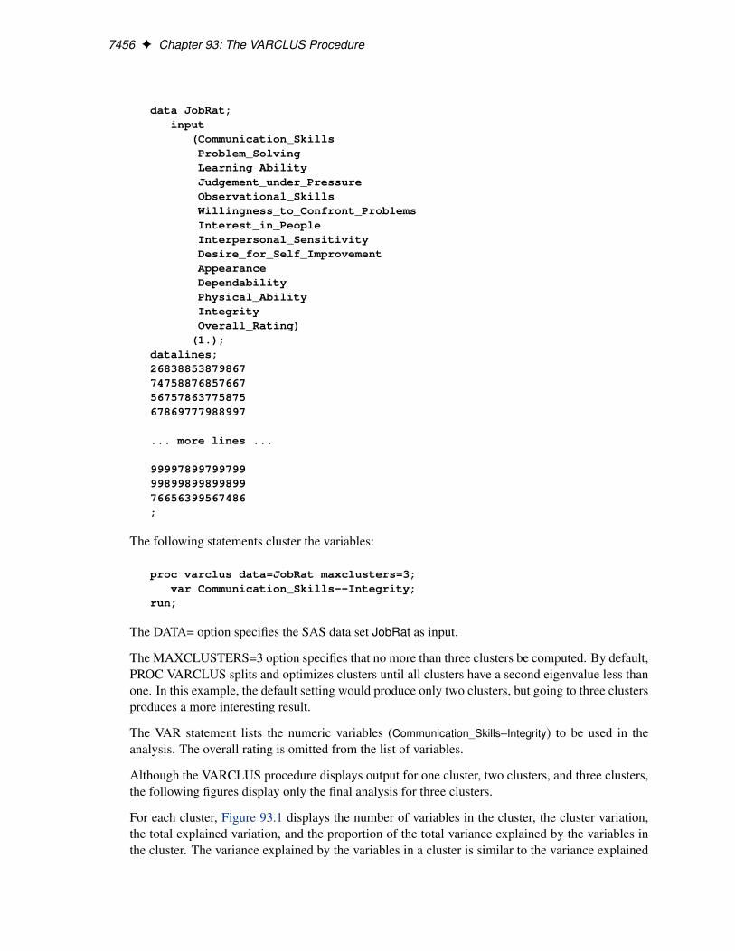
For each cluster, Figure 93.1 displays the number of variables in the cluster, the cluster variation,the total explained variation, and the proportion of the total variance explained by the variables inthe cluster. The variance explained by the variables in a cluster is similar to the variance explained


by a factor in common factor analysis, but it includes contributions only from the variables in thecluster rather than from all variables.

The line labeled “Total variation explained” in Figure 93.1 gives the sum of the explained variationover all clusters. The final “Proportion” represents the total explained variation divided by the sumof cluster variation. This value, 0.6715, indicates that about 67% of the total variation in the datacan be accounted for by the three cluster components.

Figure 93.1 Cluster Summary for Three Clusters from the VARCLUS Procedure

Oblique Principal Component Cluster Analysis

Cluster Summary for 3 Clusters

Cluster Variation Proportion SecondCluster Members Variation Explained Explained Eigenvalue------------------------------------------------------------------------

1 6 6 3.771349 0.6286 0.70932 5 5 3.575933 0.7152 0.50353 2 2 1.382005 0.6910 0.6180

Total variation explained = 8.729286 Proportion = 0.6715

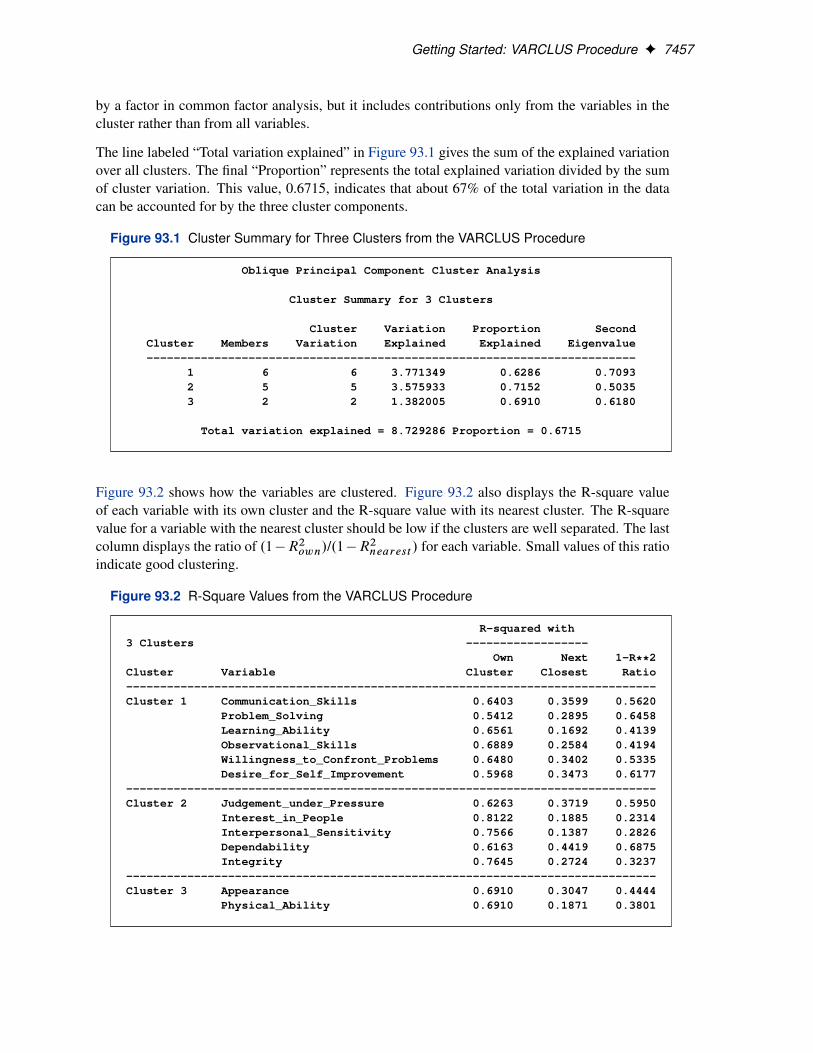
Figure 93.2 shows how the variables are clustered. Figure 93.2 also displays the R-square valueof each variable with its own cluster and the R-square value with its nearest cluster. The R-squarevalue for a variable with the nearest cluster should be low if the clusters are well separated. The lastcolumn displays the ratio of .1 � R2

own//.1 � R2nearest / for each variable. Small values of this ratio

indicate good clustering.

Figure 93.2 R-Square Values from the VARCLUS Procedure

R-squared with3 Clusters ------------------

Own Next 1-R**2Cluster Variable Cluster Closest Ratio------------------------------------------------------------------------------Cluster 1 Communication_Skills 0.6403 0.3599 0.5620

Problem_Solving 0.5412 0.2895 0.6458Learning_Ability 0.6561 0.1692 0.4139Observational_Skills 0.6889 0.2584 0.4194Willingness_to_Confront_Problems 0.6480 0.3402 0.5335Desire_for_Self_Improvement 0.5968 0.3473 0.6177

------------------------------------------------------------------------------Cluster 2 Judgement_under_Pressure 0.6263 0.3719 0.5950

Interest_in_People 0.8122 0.1885 0.2314Interpersonal_Sensitivity 0.7566 0.1387 0.2826Dependability 0.6163 0.4419 0.6875Integrity 0.7645 0.2724 0.3237

------------------------------------------------------------------------------Cluster 3 Appearance 0.6910 0.3047 0.4444

Physical_Ability 0.6910 0.1871 0.3801


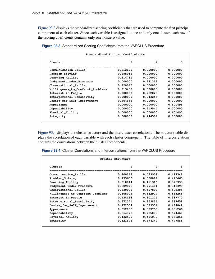
Figure 93.3 displays the standardized scoring coefficients that are used to compute the first principalcomponent of each cluster. Since each variable is assigned to one and only one cluster, each row ofthe scoring coefficients contains only one nonzero value.

Figure 93.3 Standardized Scoring Coefficients from the VARCLUS Procedure

Standardized Scoring Coefficients

Cluster 1 2 3--------------------------------------------------------------------------Communication_Skills 0.212170 0.000000 0.000000Problem_Solving 0.195058 0.000000 0.000000Learning_Ability 0.214781 0.000000 0.000000Judgement_under_Pressure 0.000000 0.221313 0.000000Observational_Skills 0.220086 0.000000 0.000000Willingness_to_Confront_Problems 0.213452 0.000000 0.000000Interest_in_People 0.000000 0.252025 0.000000Interpersonal_Sensitivity 0.000000 0.243245 0.000000Desire_for_Self_Improvement 0.204848 0.000000 0.000000Appearance 0.000000 0.000000 0.601493Dependability 0.000000 0.219544 0.000000Physical_Ability 0.000000 0.000000 0.601493Integrity 0.000000 0.244507 0.000000

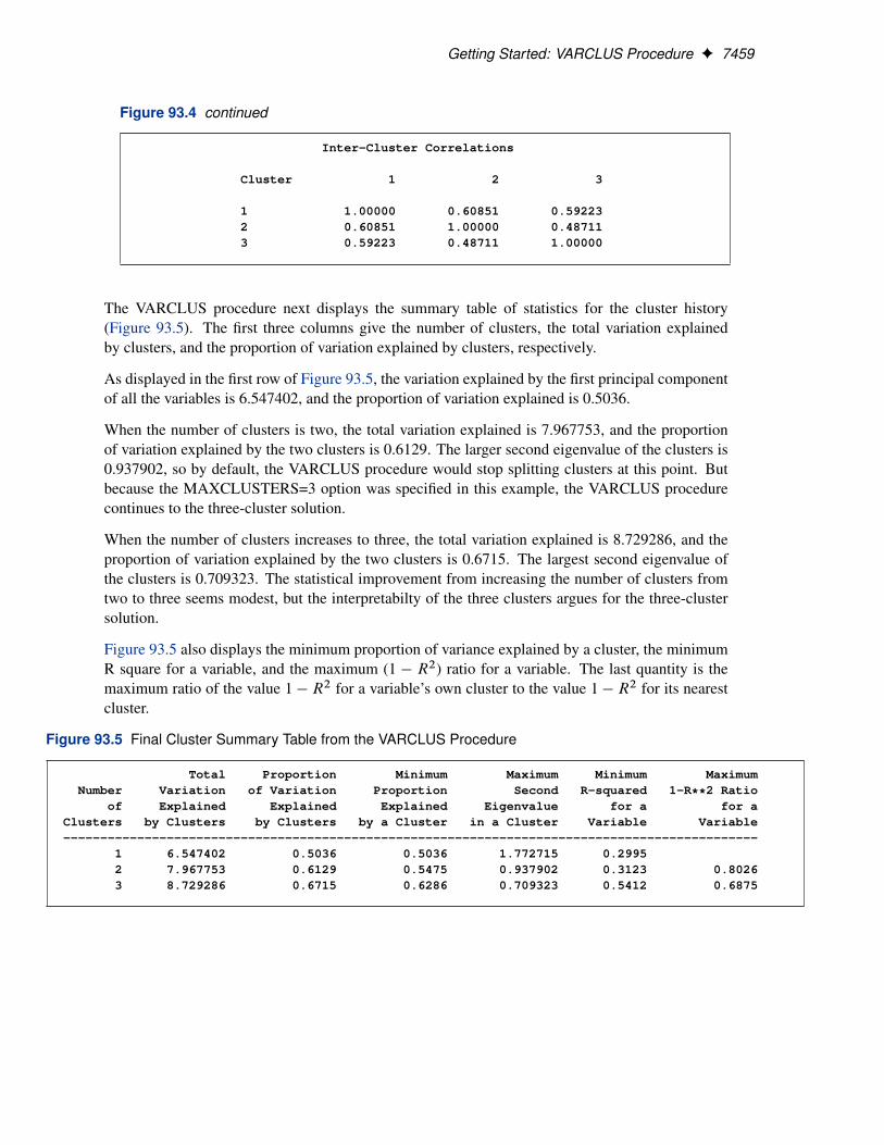
Figure 93.4 displays the cluster structure and the intercluster correlations. The structure table dis-plays the correlation of each variable with each cluster component. The table of intercorrelationscontains the correlations between the cluster components.

Figure 93.4 Cluster Correlations and Intercorrelations from the VARCLUS Procedure

Cluster Structure

Cluster 1 2 3--------------------------------------------------------------------------Communication_Skills 0.800169 0.599909 0.427341Problem_Solving 0.735630 0.538017 0.425463Learning_Ability 0.810014 0.411316 0.376333Judgement_under_Pressure 0.609876 0.791401 0.345399Observational_Skills 0.830021 0.407807 0.508305Willingness_to_Confront_Problems 0.805002 0.362927 0.583265Interest_in_People 0.434138 0.901225 0.387770Interpersonal_Sensitivity 0.372371 0.869826 0.287658Desire_for_Self_Improvement 0.772554 0.589334 0.494842Appearance 0.552003 0.393759 0.831266Dependability 0.664778 0.785073 0.574460Physical_Ability 0.432590 0.416070 0.831266Integrity 0.521876 0.874342 0.477885


Figure 93.4 continued

Inter-Cluster Correlations

Cluster 1 2 3

1 1.00000 0.60851 0.592232 0.60851 1.00000 0.487113 0.59223 0.48711 1.00000

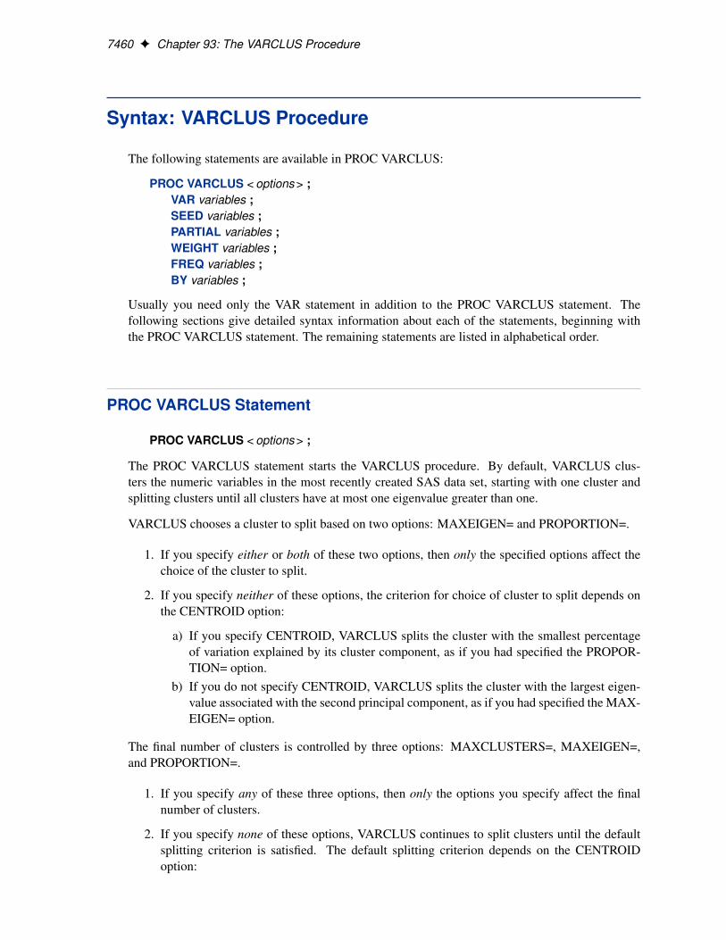
The VARCLUS procedure next displays the summary table of statistics for the cluster history(Figure 93.5). The first three columns give the number of clusters, the total variation explainedby clusters, and the proportion of variation explained by clusters, respectively.

As displayed in the first row of Figure 93.5, the variation explained by the first principal componentof all the variables is 6.547402, and the proportion of variation explained is 0.5036.

When the number of clusters is two, the total variation explained is 7.967753, and the proportionof variation explained by the two clusters is 0.6129. The larger second eigenvalue of the clusters is0.937902, so by default, the VARCLUS procedure would stop splitting clusters at this point. Butbecause the MAXCLUSTERS=3 option was specified in this example, the VARCLUS procedurecontinues to the three-cluster solution.

When the number of clusters increases to three, the total variation explained is 8.729286, and theproportion of variation explained by the two clusters is 0.6715. The largest second eigenvalue ofthe clusters is 0.709323. The statistical improvement from increasing the number of clusters fromtwo to three seems modest, but the interpretabilty of the three clusters argues for the three-clustersolution.

Figure 93.5 also displays the minimum proportion of variance explained by a cluster, the minimumR square for a variable, and the maximum (1 � R2) ratio for a variable. The last quantity is themaximum ratio of the value 1 � R2 for a variable’s own cluster to the value 1 � R2 for its nearestcluster.

Figure 93.5 Final Cluster Summary Table from the VARCLUS Procedure

Total Proportion Minimum Maximum Minimum MaximumNumber Variation of Variation Proportion Second R-squared 1-R**2 Ratio

of Explained Explained Explained Eigenvalue for a for aClusters by Clusters by Clusters by a Cluster in a Cluster Variable Variable----------------------------------------------------------------------------------------------

1 6.547402 0.5036 0.5036 1.772715 0.29952 7.967753 0.6129 0.5475 0.937902 0.3123 0.80263 8.729286 0.6715 0.6286 0.709323 0.5412 0.6875


Syntax: VARCLUS Procedure

The following statements are available in PROC VARCLUS:

PROC VARCLUS < options > ;VAR variables ;SEED variables ;PARTIAL variables ;WEIGHT variables ;FREQ variables ;BY variables ;

Usually you need only the VAR statement in addition to the PROC VARCLUS statement. Thefollowing sections give detailed syntax information about each of the statements, beginning withthe PROC VARCLUS statement. The remaining statements are listed in alphabetical order.

PROC VARCLUS Statement

PROC VARCLUS < options > ;

The PROC VARCLUS statement starts the VARCLUS procedure. By default, VARCLUS clus-ters the numeric variables in the most recently created SAS data set, starting with one cluster andsplitting clusters until all clusters have at most one eigenvalue greater than one.

VARCLUS chooses a cluster to split based on two options: MAXEIGEN= and PROPORTION=.

1. If you specify either or both of these two options, then only the specified options affect thechoice of the cluster to split.

2. If you specify neither of these options, the criterion for choice of cluster to split depends onthe CENTROID option:

a) If you specify CENTROID, VARCLUS splits the cluster with the smallest percentageof variation explained by its cluster component, as if you had specified the PROPOR-TION= option.

b) If you do not specify CENTROID, VARCLUS splits the cluster with the largest eigen-value associated with the second principal component, as if you had specified the MAX-EIGEN= option.

The final number of clusters is controlled by three options: MAXCLUSTERS=, MAXEIGEN=,and PROPORTION=.

1. If you specify any of these three options, then only the options you specify affect the finalnumber of clusters.

2. If you specify none of these options, VARCLUS continues to split clusters until the defaultsplitting criterion is satisfied. The default splitting criterion depends on the CENTROIDoption:

PROC VARCLUS Statement F 7461

a) If you specify CENTROID, the default splitting criterion is PROPORTION=0.75.

b) If you do not specify CENTROID, splitting is based on the MAXEIGEN= criterion,with a default depending on the COVARIANCE option:

i. For analyzing a correlation matrix (no COVARIANCE option), the default valuefor MAXEIGEN= is one.

ii. For analyzing a covariance matrix (using the COVARIANCE option), the defaultvalue for MAXEIGEN= is the average variance of the variables being clustered.

VARCLUS continues to split clusters until any of the following conditions holds:

� The number of cluster equals the value specified for MAXCLUSTERS=.

� No cluster qualifies for splitting according to the MAXEIGEN= or PROPORTION= criterion.

� A cluster was chosen for splitting, but after iteratively reassigning variables to clusters, oneof the cluster has no members.

Table 93.1 summarizes the options available in the PROC VARCLUS statement.

Table 93.1 Options Available in the PROC VARCLUS Statement

Option Description

Data SetsDATA= specifies the input SAS data setOUTSTAT= specifies the output SAS data set containing statisticsOUTTREE= specifies the output SAS data set for use with PROC TREE

Input Data ProcessingCOVARIANCE uses the covariance matrix instead of the correlation matrixNOINT omits interceptVARDEF= specifies the divisor for variances

Number of ClustersMAXCLUSTERS= specifies the maximum number of clustersMINCLUSTERS= specifies the minimum number of clustersMAXEIGEN= specifies the maximum second eigenvalue in a clusterPROPORTION= specifies the minimum proportion of variance explained by a cluster component

Clustering MethodsCENTROID uses centroid components instead of principal componentsHIERARCHY clusters hierarchicallyINITIAL= specifies the initialization methodMAXITER= specifies the maximum iterations during the alternating least-squares phaseMAXSEARCH= specifies the maximum iterations during the search phaseMULTIPLEGROUP performs a multiple group component analysisRANDOM= specifies the random number seed

Control Displayed OutputCORR displays the correlation matrixNOPRINT suppresses displayed output


Table 93.1 continued

Option Description

SHORT suppresses display of large matricesSIMPLE displays means and standard deviationsSUMMARY suppresses all default displayed output except the final summary tableTRACE displays the cluster to which each variable is assigned during the iterations

The following list gives details on these options. The list is in alphabetical order.

CENTROIDuses centroid components rather than principal components. You should specify centroidcomponents if you want the cluster components to be unweighted averages of the standardizedvariables (the default) or the unstandardized variables (if you specify the COVARIANCEoption). It is possible to obtain locally optimal clusterings in which a variable is not assignedto the cluster component with which it has the highest squared correlation. You cannot specifyboth the CENTROID and MAXEIGEN= options.

CORRC

displays the correlation matrix.

COVARIANCECOV

analyzes the covariance matrix instead of the correlation matrix. The COVARIANCE optioncauses variables with a large variance to have more effect on the cluster components thanvariables with a small variance.

DATA=SAS-data-setspecifies the input data set to be analyzed. The data set can be an ordinary SAS data set orTYPE=CORR, UCORR, COV, UCOV, FACTOR, or SSCP. If you do not specify the DATA=option, the most recently created SAS data set is used. See Appendix A, “Special SAS DataSets,” for more information about types of SAS data sets.

HIERARCHYHI

requires the clusters at different levels to maintain a hierarchical structure. To draw a treediagram, use the OUTTREE= option and the TREE procedure.

INITIAL=GROUPINITIAL=INPUTINITIAL=RANDOMINITIAL=SEED

specifies the method for initializing the clusters. If the INITIAL= option is omitted andthe MINCLUSTERS= option is greater than 1, the initial cluster components are obtainedby extracting the required number of principal components and performing an orthobliquerotation (raw quartimax rotation on the eigenvectors; Harris and Kaiser 1964). The followinglist describes the values for the INITIAL= option:


GROUP obtains the cluster membership of each variable from an observation in theDATA= data set where the _TYPE_ variable has a value of “GROUP”. Inthis observation, the variables to be clustered must each have an integervalue ranging from one to the number of clusters. You can use this optiononly if the DATA= data set is a TYPE=CORR, UCORR, COV, UCOV, orFACTOR data set. You can use a data set created either by a previous runof PROC VARCLUS or in a DATA step.

INPUT obtains scoring coefficients for the cluster components from observationsin the DATA= data set where the _TYPE_ variable has a value of “SCORE”.You can use this option only if the DATA= data set is a TYPE=CORR,UCORR, COV, UCOV, or FACTOR data set, You can use scoring coeffi-cients from the FACTOR procedure or a previous run of the VARCLUSprocedure, or you can enter other coefficients in a DATA step.

RANDOM assigns variables randomly to clusters.

SEED initializes each cluster component to be one of the variables named in theSEED statement. Each variable listed in the SEED statement becomes thesole member of a cluster, and the other variables are initially unassigned.If you do not specify the SEED statement, the first MINCLUSTERS= vari-ables in the VAR statement are used as seeds.

MAXCLUSTERS=n

MAXC=nspecifies the largest number of clusters desired. The default value is the number of vari-ables. VARCLUS stops splitting clusters after the number of clusters reaches the value of theMAXCLUSTERS= option, regardless of what other splitting options are specified.

MAXEIGEN=nspecifies that when choosing a cluster to split, VARCLUS should choose the cluster withthe largest second eigenvalue, provided that its second eigenvalue is greater than the MAX-EIGEN= value. The MAXEIGEN= option cannot be used with the CENTROID or MULTI-PLEGROUP options.

If you do not specify MAXEIGEN=, the default behavior depends on other options as follows:

� If you specify PROPORTION=, CENTROID, or MULTIPLEGROUP, cluster splittingdoes not depend on the second eigenvalue.

� Otherwise, if you specify MAXCLUSTERS=, the default value for MAXEIGEN= iszero.

� Otherwise, the default value for MAXEIGEN= is either 1.0 if the correlation matrix isanalyzed, or the average variance if the COVARIANCE option is specified.

If you specify both MAXEIGEN= and MAXCLUSTERS=, the number of clusters will neverexceed the value of the MAXCLUSTERS= option.

If you specify both MAXEIGEN= and PROPORTION=, VARCLUS first looks for a clusterto split based on the MAXEIGEN= criterion. If no cluster meets that criterion, VARCLUSthen looks for a cluster to split based on the PROPORTION= criterion.


MAXITER=nspecifies the maximum number of iterations during the NCS phase. The default value is 1 ifyou specify the CENTROID option; the default is 10 otherwise.

MAXSEARCH=nspecifies the maximum number of iterations during the search phase. The default is 1000divide by the number of variables.

MINCLUSTERS=n

MINC=nspecifies the smallest number of clusters desired. The default value is 2 for INI-

TIAL=RANDOM or INITIAL=SEED; otherwise, VARCLUS begins with one cluster andtries to split it in accordance with the PROPORTION= and/or MAXEIGEN= options.

MULTIPLEGROUP

MGperforms a multiple group component analysis (Harman 1976). You specify which variablesbelong to which clusters. No clusters are split, and no variables are reassigned to a differ-ent cluster. The input data set must be TYPE=CORR, UCORR, COV, UCOV, FACTOR, orSSCP and must contain an observation with _TYPE_=“GROUP” defining the variable groups.Specifying the MULTIPLEGROUP option is equivalent to specifying all of the followingoptions: INITIAL=GROUP, MINC=1, MAXITER=0, MAXSEARCH=0, PROPORTION=0,and MAXEIGEN=large number.

NOINTrequests that no intercept be used; covariances or correlations are not corrected for the mean.If you specify the NOINT option, the OUTSTAT= data set is TYPE=UCORR.

NOPRINTsuppresses displayed output. Note that this option temporarily disables the Output DeliverySystem (ODS). For more information, see Chapter 20, “Using the Output Delivery System.”

OUTSTAT=SAS-data-setcreates an output data set to contain statistics including means, standard deviations, correla-tions, cluster scoring coefficients, and the cluster structure. If you want to create a permanentSAS data set, you must specify a two-level name. The OUTSTAT= data set is TYPE=UCORRif the NOINT option is specified. For more information about permanent SAS data sets, see“SAS Files” and “DATA Step Concepts” in SAS Language Reference: Concepts. For infor-mation about types of SAS data sets, see Appendix A, “Special SAS Data Sets.”

OUTTREE=SAS-data-setcreates an output data set to contain information on the tree structure that can be used by theTREE procedure to display a tree diagram. The OUTTREE= option implies the HIERAR-CHY option. See Example 93.1 for use of the OUTTREE= option. If you want to create apermanent SAS data set, you must specify a two-level name. For more information on perma-nent SAS data sets, see “SAS Files” and “DATA Step Concepts” in SAS Language Reference:Concepts.


PROPORTION=n

PERCENT=nspecifies that when choosing a cluster to split, VARCLUS should choose the cluster with

the smallest proportion of variation explained, provided that its proportion of variation ex-plained is less than the PROPORTION= value. Values greater than 1.0 are considered to bepercentages, so PROPORTION=0.75 and PERCENT=75 are equivalent.

However, if you specify both MAXEIGEN= and PROPORTION=, VARCLUS first looks fora cluster to split based on the MAXEIGEN= criterion. If no cluster meets that criterion,VARCLUS then looks for a cluster to split based on the PROPORTION= criterion.

If you do not specify PROPORTION=, the default behavior depends on other options asfollows:

� If you specify MAXEIGEN=, cluster splitting does not depend on the proportion ofvariation explained.

� Otherwise, if you specify CENTROID and MAXCLUSTERS=, the default value forPROPORTION= is one.

� Otherwise, if you specify CENTROID, without MAXCLUSTERS=, the default value isPROPORTION=0.75 or PERCENT=75.

� Otherwise, cluster splitting does not depend on the proportion of variation explained.

If you specify both PROPORTION= and MAXCLUSTERS=, the number of clusters willnever exceed the value of the MAXCLUSTERS= option.

RANDOM=nspecifies a positive integer as a starting value for use with REPLACE=RANDOM. If you donot specify the RANDOM= option, the time of day is used to initialize the pseudo-randomnumber sequence.

SHORTsuppresses display of the cluster structure, scoring coefficient, and intercluster correlationmatrices.

SIMPLE

Sdisplays means and standard deviations.

SUMMARYsuppresses all default displayed output except the final summary table.

TRACEdisplays the cluster to which each variable is assigned during the iterations.


VARDEF=DF

VARDEF=N

VARDEF=WDF

VARDEF=WEIGHT | WGTspecifies the divisor to be used in the calculation of variances and covariances. The defaultvalue is VARDEF=DF. The values and associated divisors are displayed in the followingtable.

Value Divisor FormulaDF degrees of freedom n � i

N number of observations n

WDF sum of weights minus one .P

j wj / � 1

WEIGHT | WGT sum of weightsP

j wj

In the preceding table, i D 0 if the NOINT option is specified, and i D 1 otherwise.

BY Statement

BY variables ;

You can specify a BY statement with PROC VARCLUS to obtain separate analyses on observationsin groups defined by the BY variables. When a BY statement appears, the procedure expects theinput data set to be sorted in order of the BY variables.

If your input data set is not sorted in ascending order, use one of the following alternatives:

� Sort the data by using the SORT procedure with a similar BY statement.

� Specify the BY statement option NOTSORTED or DESCENDING in the BY statement forPROC VARCLUS. The NOTSORTED option does not mean that the data are unsorted butrather that the data are arranged in groups (according to values of the BY variables) and thatthese groups are not necessarily in alphabetical or increasing numeric order.

� Create an index on the BY variables by using the DATASETS procedure.

For more information about the BY statement, see SAS Language Reference: Concepts. For moreinformation about the DATASETS procedure, see the Base SAS Procedures Guide.

FREQ Statement

FREQ variable ;

If a variable in your data set represents the frequency of occurrence for the other values in theobservation, include the variable’s name in a FREQ statement. The procedure then treats the data set

PARTIAL Statement F 7467

as if each observation appears n times, where n is the value of the FREQ variable for the observation.If the value of the FREQ variable is less than 1, the observation is not used in the analysis. Onlythe integer portion of the value is used. The total number of observations is considered equal to thesum of the FREQ variable.

PARTIAL Statement

PARTIAL variable ;

If you want to base the clustering on partial correlations, list the variables to be partialed out in thePARTIAL statement.

SEED Statement

SEED variables ;

The SEED statement specifies variables to be used as seeds to initialize the clusters. It is notnecessary to use INITIAL=SEED if the SEED statement is present, but if any other INITIAL=option is specified, the SEED statement is ignored.

VAR Statement

VAR variables ;

The VAR statement specifies the variables to be clustered. If you do not specify the VAR statementand do not specify TYPE=SSCP, all numeric variables not listed in other statements (except theSEED statement) are processed. The default VAR variable list does not include the variable INTER-CEPT if the DATA= data set is TYPE=SSCP. If the variable INTERCEPT is explicitly specified in theVAR statement with a TYPE=SSCP data set, the NOINT option is enabled.

WEIGHT Statement

WEIGHT variables ;

If you want to specify relative weights for each observation in the input data set, place the weightsin a variable in the data set and specify the name in a WEIGHT statement. This is often done whenthe variance associated with each observation is different and the values of the weight variable areproportional to the reciprocals of the variances. The WEIGHT variable can take nonintegral values.An observation is used in the analysis only if the value of the WEIGHT variable is greater than zero.


Details: VARCLUS Procedure

Missing Values

Observations containing missing values are omitted from the analysis.

Using the VARCLUS procedure

Default options for the VARCLUS procedure often provide satisfactory results. If you want tochange the final number of clusters, use one or more of the MAXCLUSTERS=, MAXEIGEN=, orPROPORTION= options. The MAXEIGEN= and PROPORTION= options usually produce similarresults but occasionally cause different clusters to be selected for splitting. The MAXEIGEN=option tends to choose clusters with a large number of variables, while the PROPORTION= optionis more likely to select a cluster with a small number of variables.

Execution time

The VARCLUS procedure usually requires more computer time than principal factor analysis, butit can be faster than some of the iterative factoring methods. If you have more than 30 variables,you might want to reduce execution time by one or more of the following methods:

� Specify the MINCLUSTERS= and MAXCLUSTERS= options if you know how many clus-ters you want.

� Specify the HIERARCHY option.

� Specify the SEED statement if you have some prior knowledge of what clusters to expect.

If computer time is not a limiting factor, you might want to try one of the following methods toobtain a better solution:

� If the clustering algorithm has not converged, specify larger values for MAXITER= andMAXSEARCH=.

� Try several factoring and rotation methods with PROC FACTOR to use as input to PROCVARCLUS.

� Run PROC VARCLUS several times, specifying INITIAL=RANDOM.

Output Data Sets F 7469

Output Data Sets

OUTSTAT= Data Set

The OUTSTAT= data set is TYPE=CORR, and it can be used as input to the SCORE procedure ora subsequent run of PROC VARCLUS. The OUSTAT= data set contains the following variables:

� BY variables

� _NCL_, a numeric variable giving the number of clusters

� _TYPE_, a character variable indicating the type of statistic the observation contains

� _NAME_, a character variable containing a variable name or a cluster name, which is of theform CLUSn, where n is the number of the cluster

� the variables that are clustered

The values of the _TYPE_ variable are listed in the following table.

Table 93.2 _TYPE_

_TYPE_ Contents

MEAN meansSTD standard deviationsUSTD uncorrected standard deviations, produced when the NOINT option is specifiedN number of observationsCORR correlationsUCORR uncorrected correlation matrix, produced when the NOINT option is specifiedMEMBERS number of members in each clusterVAREXP variance explained by each clusterPROPOR proportion of variance explained by each clusterGROUP number of the cluster to which each variable belongsRSQUARED squared multiple correlation of each variable with its cluster componentSCORE standardized scoring coefficientsUSCORE scoring coefficients to be applied without subtracting the mean from the raw

variables, produced when the NOINT option is specifiedSTRUCTUR cluster structureCCORR correlations between cluster components

The observations with _TYPE_=“MEAN”, “STD”, “N”, and “CORR” have missing values for the_NCL_ variable. All other values of the _TYPE_ variable are repeated for each cluster solution, withdifferent solutions distinguished by the value of the _NCL_ variable. If you want to specify theOUTSTAT= data set with the SCORE procedure, you can use a DATA step to select observationswith the _NCL_ variable missing or equal to the desired number of clusters as follows:


data Coef2;set Coef;if _ncl_ = . or _ncl_ = 3;drop _ncl_;

run;

proc score data=NewScore score=Coef2; run;

PROC SCORE standardizes the new data by subtracting the original variable means that are storedin the _TYPE_=’MEAN’ observations, and dividing by the original variable standard deviationsfrom the _TYPE_=’STD’ observations. Then PROC SCORE multiplies the standardized variablesby the coefficients from the _TYPE_=’SCORE’ observations to get the cluster scores.

OUTTREE= Data Set

The OUTTREE= data set contains one observation for each variable clustered plus one observationfor each cluster of two or more variables—that is, one observation for each node of the cluster tree.The total number of output observations is between n and 2n�1, where n is the number of variablesclustered.

The OUTTREE= data set contains the following variables:

� BY variables, if any

� _NAME_, a character variable giving the name of the node. If the node is a cluster, the nameis CLUSn, where n is the number of the cluster. If the node is a single variable, the variablename is used.

� _PARENT_, a character variable giving the value of _NAME_ of the parent of the node. If thenode is the root of the tree, _PARENT_ is blank.

� _LABEL_, a character variable giving the label of the node. If the node is a cluster, the labelis CLUSn, where n is the number of the cluster. If the node is a single variable, the variablelabel is used.

� _NCL_, the number of clusters

� _VAREXP_, the total variance explained by the clusters at the current level of the tree

� _PROPOR_, the total proportion of variance explained by the clusters at the current level ofthe tree

� _MINPRO_, the minimum proportion of variance explained by a cluster component

� _MAXEIG_, the maximum second eigenvalue of a cluster

Computational Resources F 7471

Computational Resources

Let

n D number of observations

v D number of variables

c D number of clusters

It is assumed that, at each stage of clustering, the clusters all contain the same number of variables.

Time

The time required for the VARCLUS procedure to analyze a given data set varies greatly dependingon the number of clusters requested, the number of iterations in both the alternating least-squaresand search phases, and whether centroid or principal components are used.

The time required to compute the correlation matrix is roughly proportional to nv2.

Default cluster initialization requires time roughly proportional to v3. Any other method of initial-ization requires time roughly proportional to cv2.

In the alternating least-squares phase, each iteration requires time roughly proportional to cv2 ifcentroid components are used or�

c C 5v

c2

�v2

if principal components are used.

In the search phase, each iteration requires time roughly proportional to v3=c if centroid componentsare used or v4=c2 if principal components are used. The HIERARCHY option speeds up eachiteration after the first split by as much as c=2.

Memory

The amount of memory, in bytes, needed by the VARCLUS procedure is approximately

v2C 2vc C 20v C 15c

Interpreting VARCLUS Procedure Output

Because the VARCLUS algorithm is a type of oblique component analysis, its output is similarto the output from the FACTOR procedure for oblique rotations. The scoring coefficients havethe same meaning in both PROC VARCLUS and PROC FACTOR; they are coefficients applied


to the standardized variables to compute component scores. The cluster structure is analogous tothe factor structure containing the correlations between each variable and each cluster component.A cluster pattern is not displayed because it would be the same as the cluster structure, exceptthat zeros would appear in the same places in which zeros appear in the scoring coefficients. Theintercluster correlations are analogous to interfactor correlations; they are the correlations amongcluster components.

The VARCLUS procedure also displays a cluster summary and a cluster listing. The cluster sum-mary gives the number of variables in each cluster and the variation explained by the cluster compo-nent. The latter is similar to the variation explained by a factor but includes contributions from onlythe variables in that cluster rather than from all variables, as in PROC FACTOR. The proportion ofvariance explained is obtained by dividing the variance explained by the total variance of variablesin the cluster. If the cluster contains two or more variables and the CENTROID option is not used,the second largest eigenvalue of the cluster is also displayed.

The cluster listing gives the variables in each cluster. Two squared correlations are calculated foreach cluster. The column labeled “Own Cluster” gives the squared correlation of the variable withits own cluster component. This value should be higher than the squared correlation with any othercluster unless an iteration limit has been exceeded or the CENTROID option has been used. Thelarger the squared correlation is, the better. The column labeled “Next Closest” contains the next-highest squared correlation of the variable with a cluster component. This value is low if the clustersare well separated. The column labeled “1–R**2 Ratio” gives the ratio of one minus the “OwnCluster” R square to one minus the “Next Closest” R square. A small “1–R**2 Ratio” indicates agood clustering.

Displayed Output

The following items are displayed for each cluster solution unless the NOPRINT or SUMMARYoption is specified. The CLUSTER SUMMARY table includes the following columns:

� the Cluster number

� Members, the number of members in the cluster

� Cluster Variation of the variables in the cluster

� Variation Explained by the cluster component. This statistic is based only on the variables inthe cluster rather than on all variables.

� Proportion Explained, the result of dividing the variation explained by the cluster variation

� Second Eigenvalue, the second largest eigenvalue of the cluster. This is displayed if thecluster contains more than one variable and the CENTROID option is not specified

The VARCLUS procedure also displays the following:

� Total variation explained, the sum across clusters of the variation explained by each cluster

ODS Table Names F 7473

� Proportion, the total explained variation divided by the total variation of all the variables

The cluster listing includes the following columns:

� Variable, the variables in each cluster

� R square with Own Cluster, the squared correlation of the variable with its own cluster com-ponent; and R square with Next Closest, the next highest squared correlation of the variablewith a cluster component. Own Cluster values should be higher than the R square with anyother cluster unless an iteration limit is exceeded or you specify the CENTROID option. NextClosest should be a low value if the clusters are well separated.

� 1�R**2 Ratio, the ratio of one minus the value in the Own Cluster column to one minusthe value in the Next Closest column. The occurrence of low ratios indicates well-separatedclusters.

If the SHORT option is not specified, the VARCLUS procedure also displays the following tables:

� Standardized Scoring Coefficients, standardized regression coefficients for predicting clustercomponents from variables

� Cluster Structure, the correlations between each variable and each cluster component

� Inter-Cluster Correlations, the correlations between the cluster components

If the analysis includes partitions for two or more numbers of clusters, a final summary table isdisplayed. Each row of the table corresponds to one partition. The columns include the following:

� Number of Clusters

� Total Variation Explained by Clusters

� Proportion of Variation Explained by Clusters

� Minimum Proportion (of variation) Explained by a Cluster

� Maximum Second Eigenvalue in a Cluster

� Minimum R square for a Variable

� Maximum 1�R**2 Ratio for a Variable

ODS Table Names

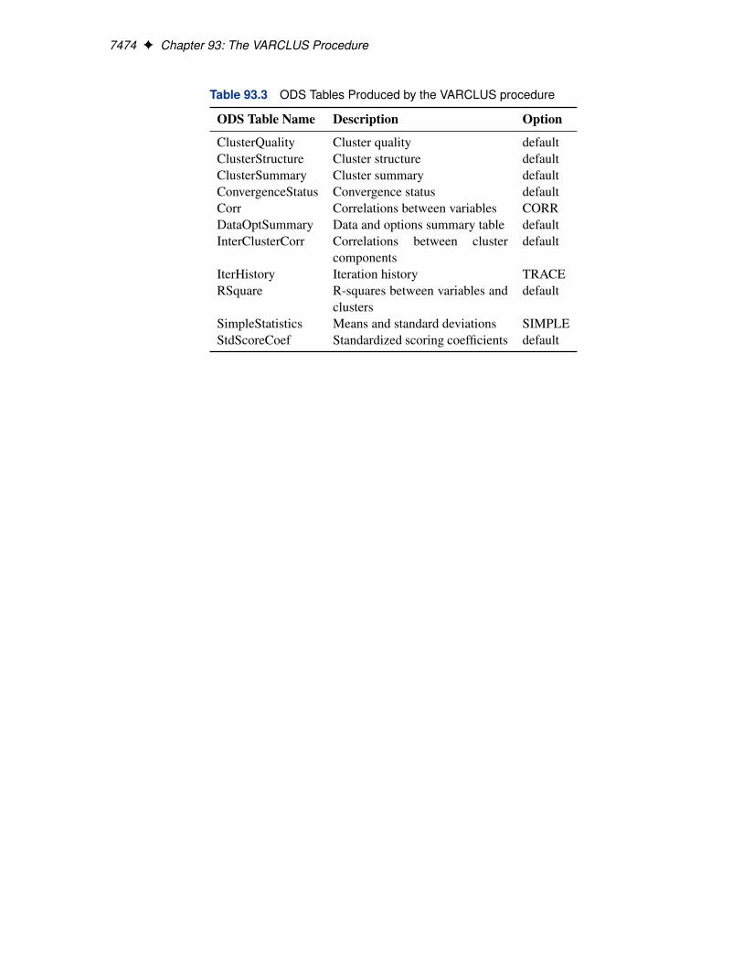
The VARCLUS procedure assigns a name to each table it creates. You can use these names toreference the table when using the Output Delivery System (ODS) to select tables and create outputdata sets. These ODS table names are listed in Table 93.3. For more information about ODS, seeChapter 20, “Using the Output Delivery System.”


Table 93.3 ODS Tables Produced by the VARCLUS procedure

ODS Table Name Description Option

ClusterQuality Cluster quality defaultClusterStructure Cluster structure defaultClusterSummary Cluster summary defaultConvergenceStatus Convergence status defaultCorr Correlations between variables CORRDataOptSummary Data and options summary table defaultInterClusterCorr Correlations between cluster

componentsdefault

IterHistory Iteration history TRACERSquare R-squares between variables and

clustersdefault

SimpleStatistics Means and standard deviations SIMPLEStdScoreCoef Standardized scoring coefficients default

Example: VARCLUS Procedure F 7475

Example: VARCLUS Procedure

Example 93.1: Correlations among Physical Variables

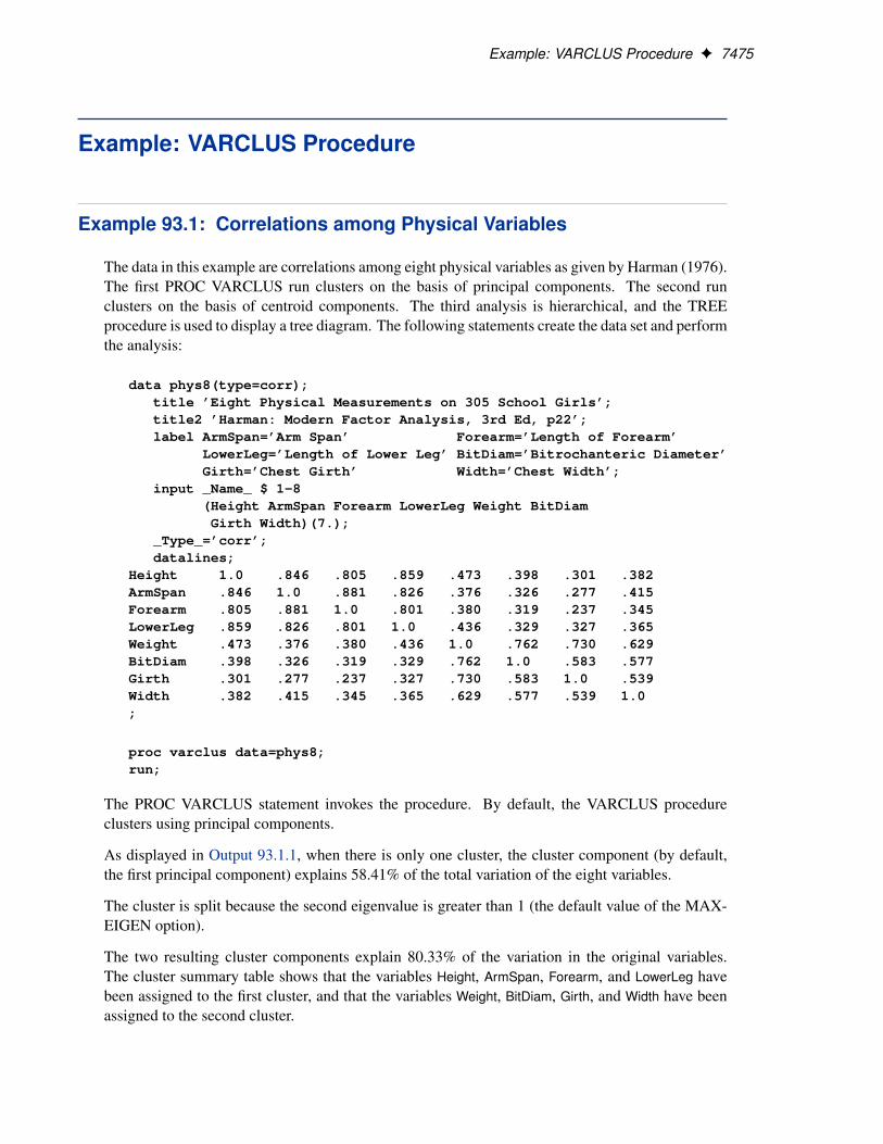
The data in this example are correlations among eight physical variables as given by Harman (1976).The first PROC VARCLUS run clusters on the basis of principal components. The second runclusters on the basis of centroid components. The third analysis is hierarchical, and the TREEprocedure is used to display a tree diagram. The following statements create the data set and performthe analysis:

data phys8(type=corr);title ’Eight Physical Measurements on 305 School Girls’;title2 ’Harman: Modern Factor Analysis, 3rd Ed, p22’;label ArmSpan=’Arm Span’ Forearm=’Length of Forearm’

LowerLeg=’Length of Lower Leg’ BitDiam=’Bitrochanteric Diameter’Girth=’Chest Girth’ Width=’Chest Width’;

input _Name_ $ 1-8(Height ArmSpan Forearm LowerLeg Weight BitDiamGirth Width)(7.);

_Type_=’corr’;datalines;

Height 1.0 .846 .805 .859 .473 .398 .301 .382ArmSpan .846 1.0 .881 .826 .376 .326 .277 .415Forearm .805 .881 1.0 .801 .380 .319 .237 .345LowerLeg .859 .826 .801 1.0 .436 .329 .327 .365Weight .473 .376 .380 .436 1.0 .762 .730 .629BitDiam .398 .326 .319 .329 .762 1.0 .583 .577Girth .301 .277 .237 .327 .730 .583 1.0 .539Width .382 .415 .345 .365 .629 .577 .539 1.0;

proc varclus data=phys8;run;

The PROC VARCLUS statement invokes the procedure. By default, the VARCLUS procedureclusters using principal components.

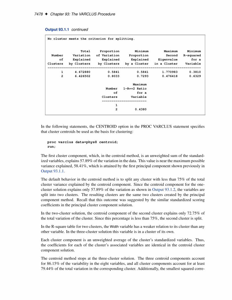
As displayed in Output 93.1.1, when there is only one cluster, the cluster component (by default,the first principal component) explains 58.41% of the total variation of the eight variables.

The cluster is split because the second eigenvalue is greater than 1 (the default value of the MAX-EIGEN option).

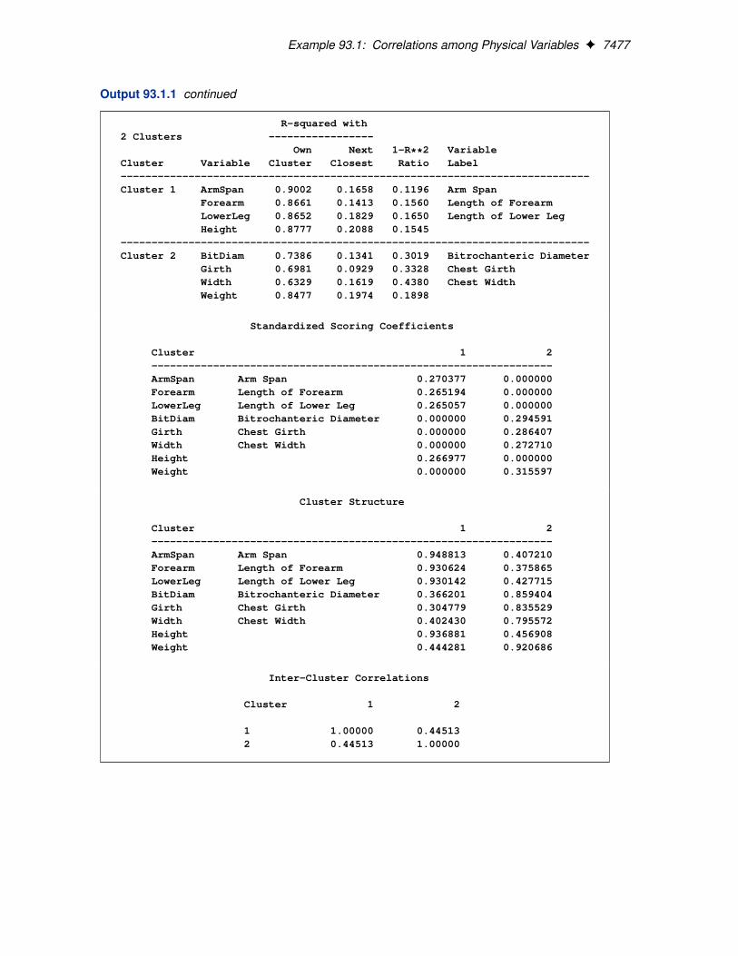
The two resulting cluster components explain 80.33% of the variation in the original variables.The cluster summary table shows that the variables Height, ArmSpan, Forearm, and LowerLeg havebeen assigned to the first cluster, and that the variables Weight, BitDiam, Girth, and Width have beenassigned to the second cluster.


The standardized scoring coefficients in Output 93.1.1 show that each cluster component has sim-ilar scores for each of its associated variables. This suggests that the principal cluster componentsolution should be similar to the centroid cluster component solution, which follows in the nextPROC VARCLUS run.

The cluster structure table displays high correlations between the variables and their own clustercomponent. The correlations between the variables and the opposite cluster component are allmoderate.

The intercluster correlation table shows that the two cluster components have a moderate correlationof 0.44513.

Output 93.1.1 Principal Component Clusters

Eight Physical Measurements on 305 School GirlsHarman: Modern Factor Analysis, 3rd Ed, p22


Observations 10000 Proportion 0Variables 8 Maxeigen 1

Clustering algorithm converged.

Cluster Summary for 1 Cluster


1 8 8 4.67288 0.5841 1.7710


Cluster 1 will be split because it has the largest second eigenvalue, 1.770983,which is greater than the MAXEIGEN=1 value.




1 4 4 3.509218 0.8773 0.23612 4 4 2.917284 0.7293 0.4764


Example 93.1: Correlations among Physical Variables F 7477

Output 93.1.1 continued

R-squared with2 Clusters -----------------

Own Next 1-R**2 VariableCluster Variable Cluster Closest Ratio Label----------------------------------------------------------------------------Cluster 1 ArmSpan 0.9002 0.1658 0.1196 Arm Span

Forearm 0.8661 0.1413 0.1560 Length of ForearmLowerLeg 0.8652 0.1829 0.1650 Length of Lower LegHeight 0.8777 0.2088 0.1545

----------------------------------------------------------------------------Cluster 2 BitDiam 0.7386 0.1341 0.3019 Bitrochanteric Diameter

Girth 0.6981 0.0929 0.3328 Chest GirthWidth 0.6329 0.1619 0.4380 Chest WidthWeight 0.8477 0.1974 0.1898


Cluster 1 2-----------------------------------------------------------------ArmSpan Arm Span 0.270377 0.000000Forearm Length of Forearm 0.265194 0.000000LowerLeg Length of Lower Leg 0.265057 0.000000BitDiam Bitrochanteric Diameter 0.000000 0.294591Girth Chest Girth 0.000000 0.286407Width Chest Width 0.000000 0.272710Height 0.266977 0.000000Weight 0.000000 0.315597

Cluster Structure



Cluster 1 2

1 1.00000 0.445132 0.44513 1.00000



No cluster meets the criterion for splitting.

Total Proportion Minimum Maximum MinimumNumber Variation of Variation Proportion Second R-squared

of Explained Explained Explained Eigenvalue for aClusters by Clusters by Clusters by a Cluster in a Cluster Variable-------------------------------------------------------------------------------

1 4.672880 0.5841 0.5841 1.770983 0.38102 6.426502 0.8033 0.7293 0.476418 0.6329

MaximumNumber 1-R**2 Ratio

of for aClusters Variable-----------------------

12 0.4380

In the following statements, the CENTROID option in the PROC VARCLUS statement specifiesthat cluster centroids be used as the basis for clustering:

proc varclus data=phys8 centroid;run;

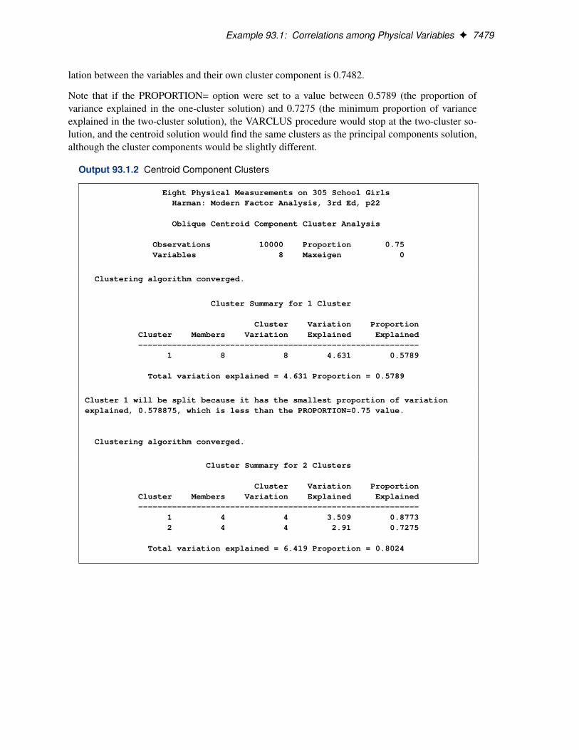
The first cluster component, which, in the centroid method, is an unweighted sum of the standard-ized variables, explains 57.89% of the variation in the data. This value is near the maximum possiblevariance explained, 58.41%, which is attained by the first principal component shown previously inOutput 93.1.1.

The default behavior in the centroid method is to split any cluster with less than 75% of the totalcluster variance explained by the centroid component. Since the centroid component for the one-cluster solution explains only 57.89% of the variation as shown in Output 93.1.2, the variables aresplit into two clusters. The resulting clusters are the same two clusters created by the principalcomponent method. Recall that this outcome was suggested by the similar standardized scoringcoefficients in the principal cluster component solution.

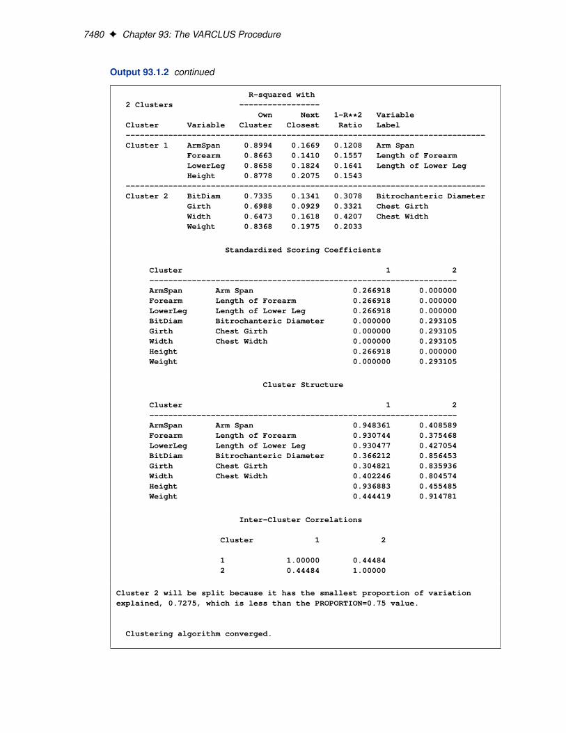
In the two-cluster solution, the centroid component of the second cluster explains only 72.75% ofthe total variation of the cluster. Since this percentage is less than 75%, the second cluster is split.

In the R-square table for two clusters, the Width variable has a weaker relation to its cluster than anyother variable. In the three-cluster solution this variable is in a cluster of its own.

Each cluster component is an unweighted average of the cluster’s standardized variables. Thus,the coefficients for each of the cluster’s associated variables are identical in the centroid clustercomponent solution.

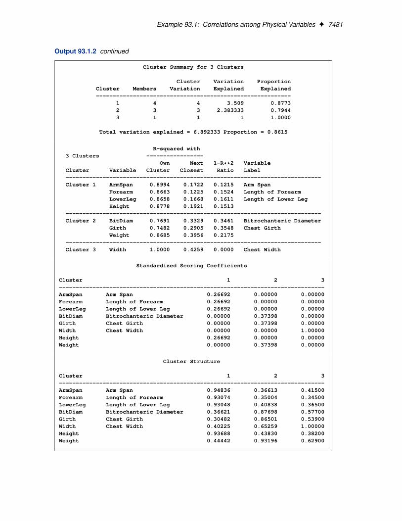
The centroid method stops at the three-cluster solution. The three centroid components accountfor 86.15% of the variability in the eight variables, and all cluster components account for at least79.44% of the total variation in the corresponding cluster. Additionally, the smallest squared corre-


lation between the variables and their own cluster component is 0.7482.

Note that if the PROPORTION= option were set to a value between 0.5789 (the proportion ofvariance explained in the one-cluster solution) and 0.7275 (the minimum proportion of varianceexplained in the two-cluster solution), the VARCLUS procedure would stop at the two-cluster so-lution, and the centroid solution would find the same clusters as the principal components solution,although the cluster components would be slightly different.

Output 93.1.2 Centroid Component Clusters


Oblique Centroid Component Cluster Analysis

Observations 10000 Proportion 0.75Variables 8 Maxeigen 0


Cluster Summary for 1 Cluster

Cluster Variation ProportionCluster Members Variation Explained Explained----------------------------------------------------------

1 8 8 4.631 0.5789


Cluster 1 will be split because it has the smallest proportion of variationexplained, 0.578875, which is less than the PROPORTION=0.75 value.




1 4 4 3.509 0.87732 4 4 2.91 0.7275








Girth 0.6988 0.0929 0.3321 Chest GirthWidth 0.6473 0.1618 0.4207 Chest WidthWeight 0.8368 0.1975 0.2033



Cluster Structure



Cluster 1 2

1 1.00000 0.444842 0.44484 1.00000

Cluster 2 will be split because it has the smallest proportion of variationexplained, 0.7275, which is less than the PROPORTION=0.75 value.






1 4 4 3.509 0.87732 3 3 2.383333 0.79443 1 1 1 1.0000






Girth 0.7482 0.2905 0.3548 Chest GirthWeight 0.8685 0.3956 0.2175

----------------------------------------------------------------------------Cluster 3 Width 1.0000 0.4259 0.0000 Chest Width


Cluster 1 2 3-------------------------------------------------------------------------------ArmSpan Arm Span 0.26692 0.00000 0.00000Forearm Length of Forearm 0.26692 0.00000 0.00000LowerLeg Length of Lower Leg 0.26692 0.00000 0.00000BitDiam Bitrochanteric Diameter 0.00000 0.37398 0.00000Girth Chest Girth 0.00000 0.37398 0.00000Width Chest Width 0.00000 0.00000 1.00000Height 0.26692 0.00000 0.00000Weight 0.00000 0.37398 0.00000

Cluster Structure

Cluster 1 2 3-------------------------------------------------------------------------------ArmSpan Arm Span 0.94836 0.36613 0.41500Forearm Length of Forearm 0.93074 0.35004 0.34500LowerLeg Length of Lower Leg 0.93048 0.40838 0.36500BitDiam Bitrochanteric Diameter 0.36621 0.87698 0.57700Girth Chest Girth 0.30482 0.86501 0.53900Width Chest Width 0.40225 0.65259 1.00000Height 0.93688 0.43830 0.38200Weight 0.44442 0.93196 0.62900




Cluster 1 2 3

1 1.00000 0.41716 0.402252 0.41716 1.00000 0.652593 0.40225 0.65259 1.00000

No cluster meets the criterion for splitting.

Total Proportion Minimum Minimum MaximumNumber Variation of Variation Proportion R-squared 1-R**2 Ratio

of Explained Explained Explained for a for aClusters by Clusters by Clusters by a Cluster Variable Variable-------------------------------------------------------------------------------

1 4.631000 0.5789 0.5789 0.43062 6.419000 0.8024 0.7275 0.6473 0.42073 6.892333 0.8615 0.7944 0.7482 0.3548

In the following statements, the MAXC= option computes all clustering solutions, from one to eightclusters. The SUMMARY option suppresses all output except the final cluster quality table, and theOUTTREE= option saves the results of the analysis to an output data set and forces the clusters tobe hierarchical. The TREE procedure is invoked to produce a graphical display of the clusters asfollows:

proc varclus data=phys8 maxc=8 summary outtree=tree;run;

title h=10pct ’Eight Physical Measurements on 305 School Girls’;title2 h=5pct ’Harman: Modern Factor Analysis, 3rd Ed, p22’;goptions htext=4pct ftext="Albany AMT";axis1 order=(0.5 to 1 by 0.1);axis2 label=none;proc tree horizontal haxis=axis1 vaxis=axis2;

height _propor_;id _label_;

run;


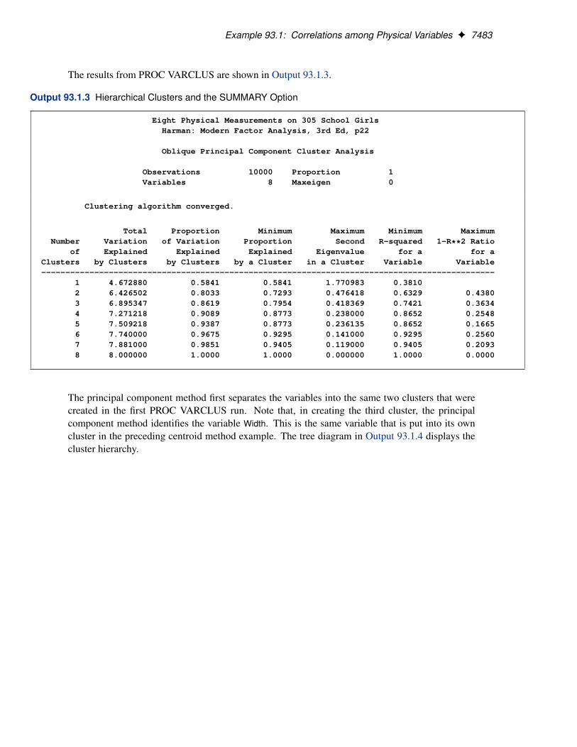
The results from PROC VARCLUS are shown in Output 93.1.3.

Output 93.1.3 Hierarchical Clusters and the SUMMARY Option



Observations 10000 Proportion 1Variables 8 Maxeigen 0


Total Proportion Minimum Maximum Minimum MaximumNumber Variation of Variation Proportion Second R-squared 1-R**2 Ratio

of Explained Explained Explained Eigenvalue for a for aClusters by Clusters by Clusters by a Cluster in a Cluster Variable Variable----------------------------------------------------------------------------------------------

1 4.672880 0.5841 0.5841 1.770983 0.38102 6.426502 0.8033 0.7293 0.476418 0.6329 0.43803 6.895347 0.8619 0.7954 0.418369 0.7421 0.36344 7.271218 0.9089 0.8773 0.238000 0.8652 0.25485 7.509218 0.9387 0.8773 0.236135 0.8652 0.16656 7.740000 0.9675 0.9295 0.141000 0.9295 0.25607 7.881000 0.9851 0.9405 0.119000 0.9405 0.20938 8.000000 1.0000 1.0000 0.000000 1.0000 0.0000

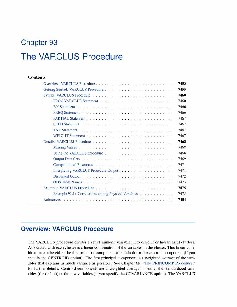
The principal component method first separates the variables into the same two clusters that werecreated in the first PROC VARCLUS run. Note that, in creating the third cluster, the principalcomponent method identifies the variable Width. This is the same variable that is put into its owncluster in the preceding centroid method example. The tree diagram in Output 93.1.4 displays thecluster hierarchy.


Output 93.1.4 Tree Diagram from PROC TREE

It appears from the diagram that there are two, or possibly three, clusters present. However, theMAXC=8 option forces the VARCLUS procedure to split the clusters until each variable is in itsown cluster.

References

Anderberg, M. R. (1973), Cluster Analysis for Applications, New York: Academic Press Inc.

Hand, D. J., Daly, F., Lunn, A. D., McConway, K. J., and Ostrowski E. (1994), A Handbook ofSmall Data Sets, London: Chapman & Hall, 297–298.

Harman, H. H. (1976), Modern Factor Analysis, Third Edition, Chicago: University of ChicagoPress.

Harris, C. W., and Kaiser, H. F. (1964), “Oblique Factor Analytic Solutions by Orthogonal Trans-formation,” Psychometrika, 32, 363–379.

Subject Index

analyzing data in groupsVARCLUS procedure, 7466

centroid component, 7455definition, 7453

clusteringdisjoint clusters of variables, 7453hierarchical clusters of variables, 7453variables, 7453

computational resourcesVARCLUS procedure, 7471

hierarchical clustering, 7455

interpreting outputVARCLUS procedure, 7471

memory requirementsVARCLUS procedure, 7471

oblique component analysis, 7454orthoblique rotation, 7454output data sets

VARCLUS procedure, 7464, 7469output table names

VARCLUS procedure, 7473

time requirementsVARCLUS procedure, 7468, 7471

VARCLUS procedurealternating least squares, 7455analyzing data in groups, 7466centroid component, 7462cluster components, 7454cluster splitting, 7454, 7455, 7460, 7463,

7465cluster, definition, 7453computational resources, 7471controlling number of clusters, 7464eigenvalues, 7454, 7455, 7463how to choose options, 7468initializing clusters, 7462interpreting output, 7471iterative reassignment, 7454, 7455MAXCLUSTERS= option, using, 7468MAXEIGEN= option, using, 7468memory requirements, 7471missing values, 7468

multiple group component analysis, 7464nearest component sorting phase, 7455number of clusters, 7454, 7455, 7460,

7463–7465orthoblique rotation, 7454, 7462output data sets, 7464, 7469output table names, 7473OUTSTAT= data set, 7464, 7469OUTTREE= data set, 7470PROPORTION= option, using, 7468search phase, 7455splitting criteria, 7454, 7455, 7460, 7463,

7465stopping criteria, 7460time requirements, 7468, 7471TYPE=CORR data set, 7469

variable-reduction method, 7454

Syntax Index

BY statementVARCLUS procedure, 7466

CENTROID optionPROC VARCLUS statement, 7462

CORR optionPROC VARCLUS statement, 7462

COVARIANCE optionPROC VARCLUS statement, 7462

DATA= optionPROC VARCLUS statement, 7462

FREQ statementVARCLUS procedure, 7466

HIERARCHY optionPROC VARCLUS statement, 7462

INITIAL= optionPROC VARCLUS statement, 7462

MAXCLUSTERS= optionPROC VARCLUS statement, 7463

MAXEIGEN= optionPROC VARCLUS statement, 7463

MAXITER= optionPROC VARCLUS statement, 7464

MAXSEARCH= optionPROC VARCLUS statement, 7464

MINC= optionPROC VARCLUS statement, 7464

MINCLUSTERS= optionPROC VARCLUS statement, 7464

MULTIPLEGROUP optionPROC VARCLUS statement, 7464

NOINT optionPROC VARCLUS statement, 7464

NOPRINT optionPROC VARCLUS statement, 7464

OUTSTAT= optionPROC VARCLUS statement, 7464

OUTTREE= optionPROC VARCLUS statement, 7464

PARTIAL statementVARCLUS procedure, 7467

PERCENT= option

PROC VARCLUS statement, 7465PROC VARCLUS statement, see VARCLUS

procedurePROPORTION= option

PROC VARCLUS statement, 7465

RANDOM= optionPROC VARCLUS statement, 7465

SEED statementVARCLUS procedure, 7467

SHORT optionPROC VARCLUS statement, 7465

SIMPLE optionPROC VARCLUS statement, 7465

SUMMARY optionPROC VARCLUS statement, 7465

TRACE optionPROC VARCLUS statement, 7465

VAR statementVARCLUS procedure, 7467

VARCLUS proceduresyntax, 7460

VARCLUS procedure, BY statement, 7466VARCLUS procedure, FREQ statement, 7466VARCLUS procedure, PARTIAL statement, 7467VARCLUS procedure, PROC VARCLUS

statement, 7460CENTROID option, 7462CORR option, 7462COVARIANCE option, 7462DATA= option, 7462HIERARCHY option, 7462INITIAL= option, 7462MAXCLUSTERS= option, 7463MAXEIGEN= option, 7463MAXITER= option, 7464MAXSEARCH= option, 7464MINC= option, 7464MINCLUSTERS= option, 7464MULTIPLEGROUP option, 7464NOINT option, 7464NOPRINT option, 7464OUTSTAT= option, 7464OUTTREE= option, 7464PERCENT= option, 7465PROPORTION= option, 7465

RANDOM= option, 7465SHORT option, 7465SIMPLE option, 7465SUMMARY option, 7465TRACE option, 7465VARDEF= option, 7466

VARCLUS procedure, SEED statement, 7467VARCLUS procedure, VAR statement, 7467VARCLUS procedure, WEIGHT statement, 7467VARDEF= option

PROC VARCLUS statement, 7466

WEIGHT statementVARCLUS procedure, 7467

Your Turn

We welcome your feedback.

� If you have comments about this book, please send them [email protected]. Include the full title and page numbers (ifapplicable).

� If you have comments about the software, please send them [email protected].

SAS® Publishing Delivers!Whether you are new to the work force or an experienced professional, you need to distinguish yourself in this rapidly changing and competitive job market. SAS® Publishing provides you with a wide range of resources to help you set yourself apart. Visit us online at support.sas.com/bookstore.

SAS® Press Need to learn the basics? Struggling with a programming problem? You’ll find the expert answers that you need in example-rich books from SAS Press. Written by experienced SAS professionals from around the world, SAS Press books deliver real-world insights on a broad range of topics for all skill levels.

s u p p o r t . s a s . c o m / s a s p r e s sSAS® Documentation To successfully implement applications using SAS software, companies in every industry and on every continent all turn to the one source for accurate, timely, and reliable information: SAS documentation. We currently produce the following types of reference documentation to improve your work experience:

• Onlinehelpthatisbuiltintothesoftware.• Tutorialsthatareintegratedintotheproduct.• ReferencedocumentationdeliveredinHTMLandPDF– free on the Web. • Hard-copybooks.

s u p p o r t . s a s . c o m / p u b l i s h i n gSAS® Publishing News Subscribe to SAS Publishing News to receive up-to-date information about all new SAS titles, author podcasts, and new Web site features via e-mail. Complete instructions on how to subscribe, as well as access to past issues, are available at our Web site.

s u p p o r t . s a s . c o m / s p n

SAS and all other SAS Institute Inc. product or service names are registered trademarks or trademarks of SAS Institute Inc. in the USA and other countries. ® indicates USA registration. Otherbrandandproductnamesaretrademarksoftheirrespectivecompanies.©2009SASInstituteInc.Allrightsreserved.518177_1US.0109

Documents

SAS/STAT 9.2 User's Guide: The VARCLUS …...® 9.2 User’s Guide The VARCLUS Procedure (Book Excerpt) SAS ® Documentation This document is an individual chapter from SAS/STAT®