Embed Size (px)
Citation preview
SAS/STAT® 9.2 User’s GuideThe ROBUSTREG Procedure(Book Excerpt)
SAS® Documentation
This document is an individual chapter from SAS/STAT® 9.2 User’s Guide.
The correct bibliographic citation for the complete manual is as follows: SAS Institute Inc. 2008. SAS/STAT® 9.2User’s Guide. Cary, NC: SAS Institute Inc.
Copyright © 2008, SAS Institute Inc., Cary, NC, USA
All rights reserved. Produced in the United States of America.
For a Web download or e-book: Your use of this publication shall be governed by the terms established by the vendorat the time you acquire this publication.
U.S. Government Restricted Rights Notice: Use, duplication, or disclosure of this software and related documentationby the U.S. government is subject to the Agreement with SAS Institute and the restrictions set forth in FAR 52.227-19,Commercial Computer Software-Restricted Rights (June 1987).
SAS Institute Inc., SAS Campus Drive, Cary, North Carolina 27513.
1st electronic book, March 20082nd electronic book, February 2009SAS® Publishing provides a complete selection of books and electronic products to help customers use SAS software toits fullest potential. For more information about our e-books, e-learning products, CDs, and hard-copy books, visit theSAS Publishing Web site at support.sas.com/publishing or call 1-800-727-3228.
SAS® and all other SAS Institute Inc. product or service names are registered trademarks or trademarks of SAS InstituteInc. in the USA and other countries. ® indicates USA registration.
Other brand and product names are registered trademarks or trademarks of their respective companies.
Chapter 74
The ROBUSTREG Procedure
ContentsOverview: ROBUSTREG Procedure . . . . . . . . . . . . . . . . . . . . . . . . . 5642
Features . . . . . . . . . . . . . . . . . . . . . . . . . . . . . . . . . . . . 5642Getting Started: ROBUSTREG Procedure . . . . . . . . . . . . . . . . . . . . . . 5643
M Estimation . . . . . . . . . . . . . . . . . . . . . . . . . . . . . . . . . . 5643LTS Estimation . . . . . . . . . . . . . . . . . . . . . . . . . . . . . . . . . 5650
Syntax: ROBUSTREG Procedure . . . . . . . . . . . . . . . . . . . . . . . . . . 5654PROC ROBUSTREG Statement . . . . . . . . . . . . . . . . . . . . . . . . 5654BY Statement . . . . . . . . . . . . . . . . . . . . . . . . . . . . . . . . . 5661CLASS Statement . . . . . . . . . . . . . . . . . . . . . . . . . . . . . . . 5662ID Statement . . . . . . . . . . . . . . . . . . . . . . . . . . . . . . . . . . 5662MODEL Statement . . . . . . . . . . . . . . . . . . . . . . . . . . . . . . . 5662OUTPUT Statement . . . . . . . . . . . . . . . . . . . . . . . . . . . . . . 5664PERFORMANCE Statement . . . . . . . . . . . . . . . . . . . . . . . . . 5665TEST Statement . . . . . . . . . . . . . . . . . . . . . . . . . . . . . . . . 5665WEIGHT Statement . . . . . . . . . . . . . . . . . . . . . . . . . . . . . . 5666
Details: ROBUSTREG Procedure . . . . . . . . . . . . . . . . . . . . . . . . . . 5666M Estimation . . . . . . . . . . . . . . . . . . . . . . . . . . . . . . . . . . 5666High Breakdown Value Estimation . . . . . . . . . . . . . . . . . . . . . . 5673MM Estimation . . . . . . . . . . . . . . . . . . . . . . . . . . . . . . . . 5678Robust Distance . . . . . . . . . . . . . . . . . . . . . . . . . . . . . . . . 5682Leverage Point and Outlier Detection . . . . . . . . . . . . . . . . . . . . . 5683INEST= Data Set . . . . . . . . . . . . . . . . . . . . . . . . . . . . . . . . 5683OUTEST= Data Set . . . . . . . . . . . . . . . . . . . . . . . . . . . . . . 5684Computational Resources . . . . . . . . . . . . . . . . . . . . . . . . . . . 5684ODS Table Names . . . . . . . . . . . . . . . . . . . . . . . . . . . . . . . 5685ODS Graphics . . . . . . . . . . . . . . . . . . . . . . . . . . . . . . . . . 5686
Examples: ROBUSTREG Procedure . . . . . . . . . . . . . . . . . . . . . . . . . 5691Example 74.1: Comparison of Robust Estimates . . . . . . . . . . . . . . . 5691Example 74.2: Robust ANOVA . . . . . . . . . . . . . . . . . . . . . . . . 5698Example 74.3: Growth Study of De Long and Summers . . . . . . . . . . . 5702
References . . . . . . . . . . . . . . . . . . . . . . . . . . . . . . . . . . . . . . 5710
5642 F Chapter 74: The ROBUSTREG Procedure
Overview: ROBUSTREG Procedure
The main purpose of robust regression is to detect outliers and provide resistant (stable) results inthe presence of outliers. In order to achieve this stability, robust regression limits the influenceof outliers. Historically, three classes of problems have been addressed with robust regressiontechniques:
� problems with outliers in the y-direction (response direction)
� problems with multivariate outliers in the x-space (i.e., outliers in the covariate space, whichare also referred to as leverage points)
� problems with outliers in both the y-direction and the x-space
Many methods have been developed in response to these problems. However, in statistical applica-tions of outlier detection and robust regression, the methods most commonly used today are HuberM estimation, high breakdown value estimation, and combinations of these two methods. The RO-BUSTREG procedure in SAS 9.2 provides four such methods: M estimation, LTS estimation, Sestimation, and MM estimation.
1. M estimation was introduced by Huber (1973), and it is the simplest approach both compu-tationally and theoretically. Although it is not robust with respect to leverage points, it isstill used extensively in analyzing data for which it can be assumed that the contamination ismainly in the response direction.
2. Least trimmed squares (LTS) estimation is a high breakdown value method introduced byRousseeuw (1984). The breakdown value is a measure of the proportion of contaminationthat an estimation method can withstand and still maintain its robustness. The performanceof this method was improved by the FAST-LTS algorithm of Rousseeuw and Van Driessen(2000).
3. S estimation is a high breakdown value method introduced by Rousseeuw and Yohai (1984).With the same breakdown value, it has a higher statistical efficiency than LTS estimation.
4. MM estimation, introduced by Yohai (1987), combines high breakdown value estimation andM estimation. It has both the high breakdown property and a higher statistical efficiency thanS estimation.
Features
The main features of the ROBUSTREG procedure are as follows:
� offers four estimation methods: M, LTS, S, and MM
Getting Started: ROBUSTREG Procedure F 5643
� provides 10 weight functions for M estimation
� provides robust R2 and deviance for all estimates
� provides asymptotic covariance and confidence intervals for regression parameter with the M,S, and MM methods
� provides robust Wald and F tests for regression parameters with the M and MM methods
� provides outlier and leverage-point diagnostics
� supports parallel computing for S and LTS estimates
� produces fit plots and diagnostic plots by using ODS Graphics
Getting Started: ROBUSTREG Procedure
The following examples demonstrate how you can use the ROBUSTREG procedure to fit a linearregression model and obtain outlier and leverage-point diagnostics.
M Estimation
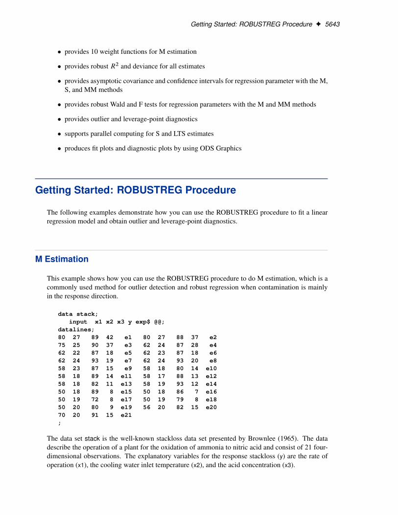
This example shows how you can use the ROBUSTREG procedure to do M estimation, which is acommonly used method for outlier detection and robust regression when contamination is mainlyin the response direction.
data stack;input x1 x2 x3 y exp$ @@;
datalines;80 27 89 42 e1 80 27 88 37 e275 25 90 37 e3 62 24 87 28 e462 22 87 18 e5 62 23 87 18 e662 24 93 19 e7 62 24 93 20 e858 23 87 15 e9 58 18 80 14 e1058 18 89 14 e11 58 17 88 13 e1258 18 82 11 e13 58 19 93 12 e1450 18 89 8 e15 50 18 86 7 e1650 19 72 8 e17 50 19 79 8 e1850 20 80 9 e19 56 20 82 15 e2070 20 91 15 e21;
The data set stack is the well-known stackloss data set presented by Brownlee (1965). The datadescribe the operation of a plant for the oxidation of ammonia to nitric acid and consist of 21 four-dimensional observations. The explanatory variables for the response stackloss (y) are the rate ofoperation (x1), the cooling water inlet temperature (x2), and the acid concentration (x3).
5644 F Chapter 74: The ROBUSTREG Procedure
The following ROBUSTREG statements analyze the data:
proc robustreg data=stack;model y = x1 x2 x3 / diagnostics leverage;id exp;test x3;
run;
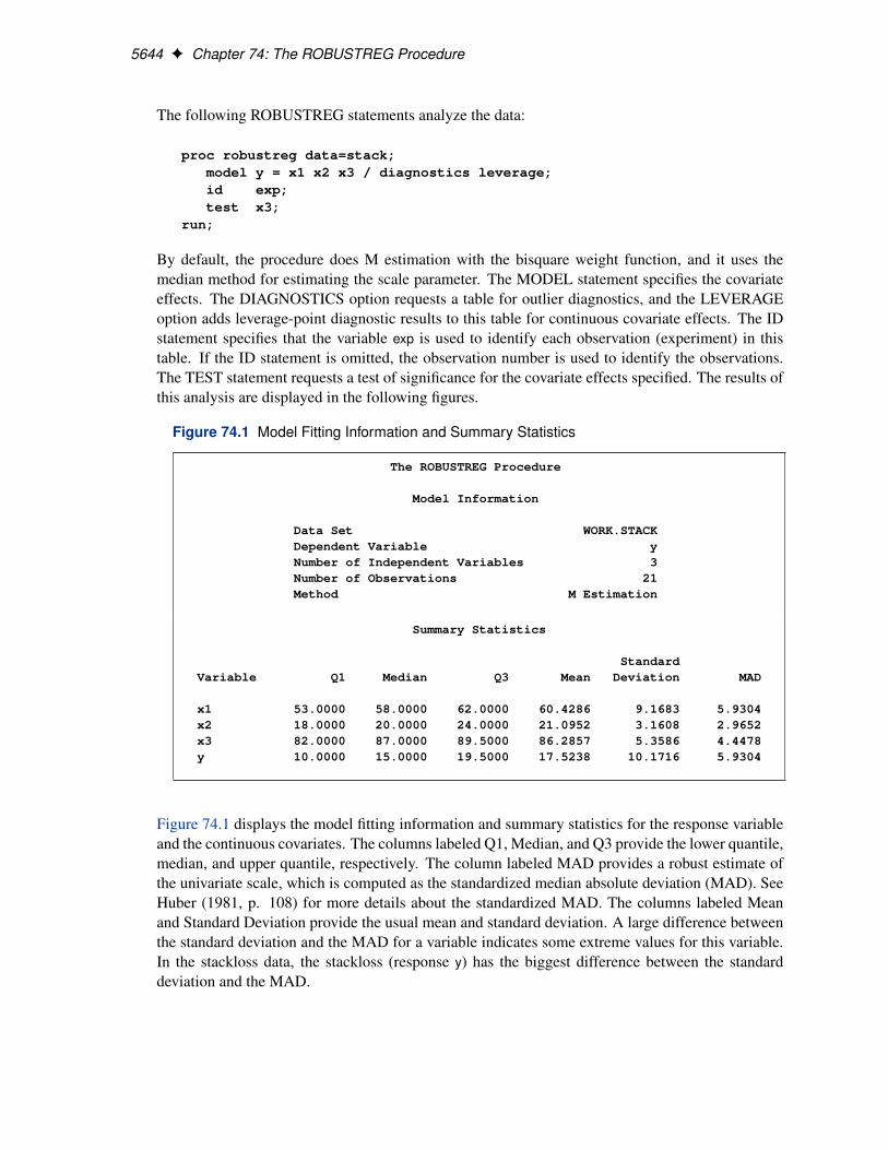
By default, the procedure does M estimation with the bisquare weight function, and it uses themedian method for estimating the scale parameter. The MODEL statement specifies the covariateeffects. The DIAGNOSTICS option requests a table for outlier diagnostics, and the LEVERAGEoption adds leverage-point diagnostic results to this table for continuous covariate effects. The IDstatement specifies that the variable exp is used to identify each observation (experiment) in thistable. If the ID statement is omitted, the observation number is used to identify the observations.The TEST statement requests a test of significance for the covariate effects specified. The results ofthis analysis are displayed in the following figures.
Figure 74.1 Model Fitting Information and Summary Statistics
The ROBUSTREG Procedure
Model Information
Data Set WORK.STACKDependent Variable yNumber of Independent Variables 3Number of Observations 21Method M Estimation
Summary Statistics
StandardVariable Q1 Median Q3 Mean Deviation MAD
x1 53.0000 58.0000 62.0000 60.4286 9.1683 5.9304x2 18.0000 20.0000 24.0000 21.0952 3.1608 2.9652x3 82.0000 87.0000 89.5000 86.2857 5.3586 4.4478y 10.0000 15.0000 19.5000 17.5238 10.1716 5.9304
Figure 74.1 displays the model fitting information and summary statistics for the response variableand the continuous covariates. The columns labeled Q1, Median, and Q3 provide the lower quantile,median, and upper quantile, respectively. The column labeled MAD provides a robust estimate ofthe univariate scale, which is computed as the standardized median absolute deviation (MAD). SeeHuber (1981, p. 108) for more details about the standardized MAD. The columns labeled Meanand Standard Deviation provide the usual mean and standard deviation. A large difference betweenthe standard deviation and the MAD for a variable indicates some extreme values for this variable.In the stackloss data, the stackloss (response y) has the biggest difference between the standarddeviation and the MAD.
M Estimation F 5645
Figure 74.2 Model Parameter Estimates
Parameter Estimates
Standard 95% Confidence Chi-Parameter DF Estimate Error Limits Square Pr > ChiSq
Intercept 1 -42.2854 9.5045 -60.9138 -23.6569 19.79 <.0001x1 1 0.9276 0.1077 0.7164 1.1387 74.11 <.0001x2 1 0.6507 0.2940 0.0744 1.2270 4.90 0.0269x3 1 -0.1123 0.1249 -0.3571 0.1324 0.81 0.3683Scale 1 2.2819
Figure 74.2 displays the table of robust parameter estimates, standard errors, and confidence limits.The row labeled Scale provides a point estimate of the scale parameter in the linear regressionmodel, which is obtained by the median method. See the section “M Estimation” on page 5666 formore information about scale estimation methods. For the stackloss data, M estimation yields thefitted linear model:
Oy D �42:2845C 0:9276x1 C 0:6507x2 � 0:1123x3
Figure 74.3 Diagnostics
Diagnostics
Robust StandardizedMahalanobis MCD Robust
Obs exp Distance Distance Leverage Residual Outlier
1 e1 2.2536 5.5284 * 1.09952 e2 2.3247 5.6374 * -1.14093 e3 1.5937 4.1972 * 1.56044 e4 1.2719 1.5887 3.0381 *
21 e21 2.1768 3.6573 * -4.5733 *
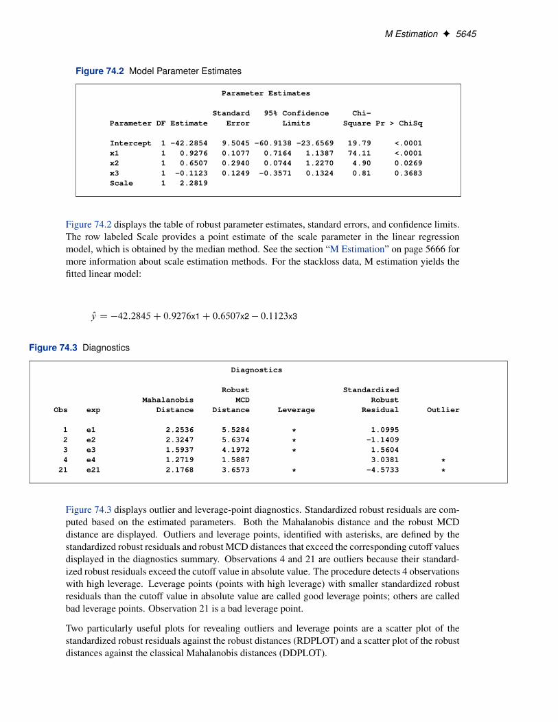
Figure 74.3 displays outlier and leverage-point diagnostics. Standardized robust residuals are com-puted based on the estimated parameters. Both the Mahalanobis distance and the robust MCDdistance are displayed. Outliers and leverage points, identified with asterisks, are defined by thestandardized robust residuals and robust MCD distances that exceed the corresponding cutoff valuesdisplayed in the diagnostics summary. Observations 4 and 21 are outliers because their standard-ized robust residuals exceed the cutoff value in absolute value. The procedure detects 4 observationswith high leverage. Leverage points (points with high leverage) with smaller standardized robustresiduals than the cutoff value in absolute value are called good leverage points; others are calledbad leverage points. Observation 21 is a bad leverage point.
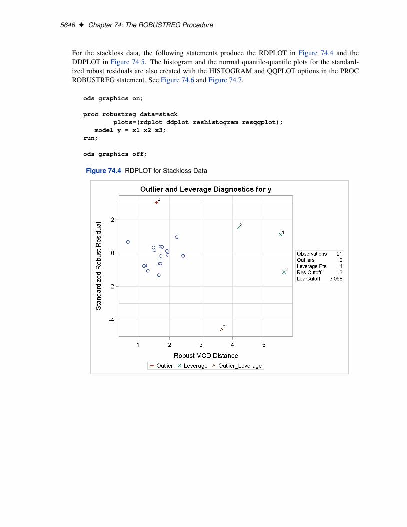
Two particularly useful plots for revealing outliers and leverage points are a scatter plot of thestandardized robust residuals against the robust distances (RDPLOT) and a scatter plot of the robustdistances against the classical Mahalanobis distances (DDPLOT).
5646 F Chapter 74: The ROBUSTREG Procedure
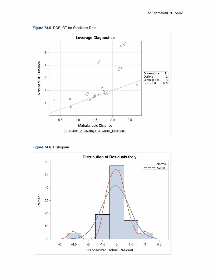
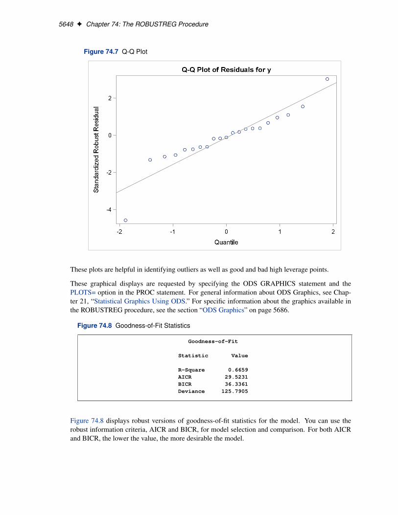
For the stackloss data, the following statements produce the RDPLOT in Figure 74.4 and theDDPLOT in Figure 74.5. The histogram and the normal quantile-quantile plots for the standard-ized robust residuals are also created with the HISTOGRAM and QQPLOT options in the PROCROBUSTREG statement. See Figure 74.6 and Figure 74.7.
ods graphics on;
proc robustreg data=stackplots=(rdplot ddplot reshistogram resqqplot);
model y = x1 x2 x3;run;
ods graphics off;
Figure 74.4 RDPLOT for Stackloss Data
M Estimation F 5647
Figure 74.5 DDPLOT for Stackloss Data
Figure 74.6 Histogram
5648 F Chapter 74: The ROBUSTREG Procedure
Figure 74.7 Q-Q Plot
These plots are helpful in identifying outliers as well as good and bad high leverage points.
These graphical displays are requested by specifying the ODS GRAPHICS statement and thePLOTS= option in the PROC statement. For general information about ODS Graphics, see Chap-ter 21, “Statistical Graphics Using ODS.” For specific information about the graphics available inthe ROBUSTREG procedure, see the section “ODS Graphics” on page 5686.
Figure 74.8 Goodness-of-Fit Statistics
Goodness-of-Fit
Statistic Value
R-Square 0.6659AICR 29.5231BICR 36.3361Deviance 125.7905
Figure 74.8 displays robust versions of goodness-of-fit statistics for the model. You can use therobust information criteria, AICR and BICR, for model selection and comparison. For both AICRand BICR, the lower the value, the more desirable the model.
M Estimation F 5649
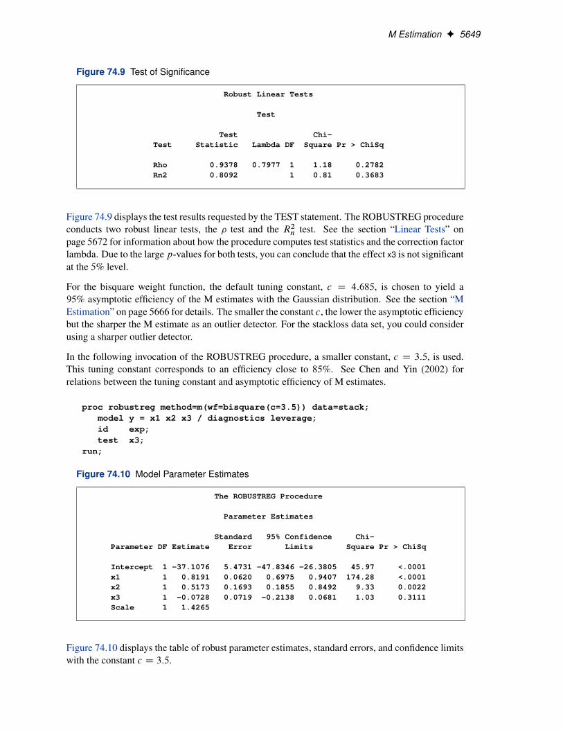
Figure 74.9 Test of Significance
Robust Linear Tests
Test
Test Chi-Test Statistic Lambda DF Square Pr > ChiSq
Rho 0.9378 0.7977 1 1.18 0.2782Rn2 0.8092 1 0.81 0.3683
Figure 74.9 displays the test results requested by the TEST statement. The ROBUSTREG procedureconducts two robust linear tests, the � test and the R2n test. See the section “Linear Tests” onpage 5672 for information about how the procedure computes test statistics and the correction factorlambda. Due to the large p-values for both tests, you can conclude that the effect x3 is not significantat the 5% level.
For the bisquare weight function, the default tuning constant, c D 4:685, is chosen to yield a95% asymptotic efficiency of the M estimates with the Gaussian distribution. See the section “MEstimation” on page 5666 for details. The smaller the constant c, the lower the asymptotic efficiencybut the sharper the M estimate as an outlier detector. For the stackloss data set, you could considerusing a sharper outlier detector.
In the following invocation of the ROBUSTREG procedure, a smaller constant, c D 3:5, is used.This tuning constant corresponds to an efficiency close to 85%. See Chen and Yin (2002) forrelations between the tuning constant and asymptotic efficiency of M estimates.
proc robustreg method=m(wf=bisquare(c=3.5)) data=stack;model y = x1 x2 x3 / diagnostics leverage;id exp;test x3;
run;
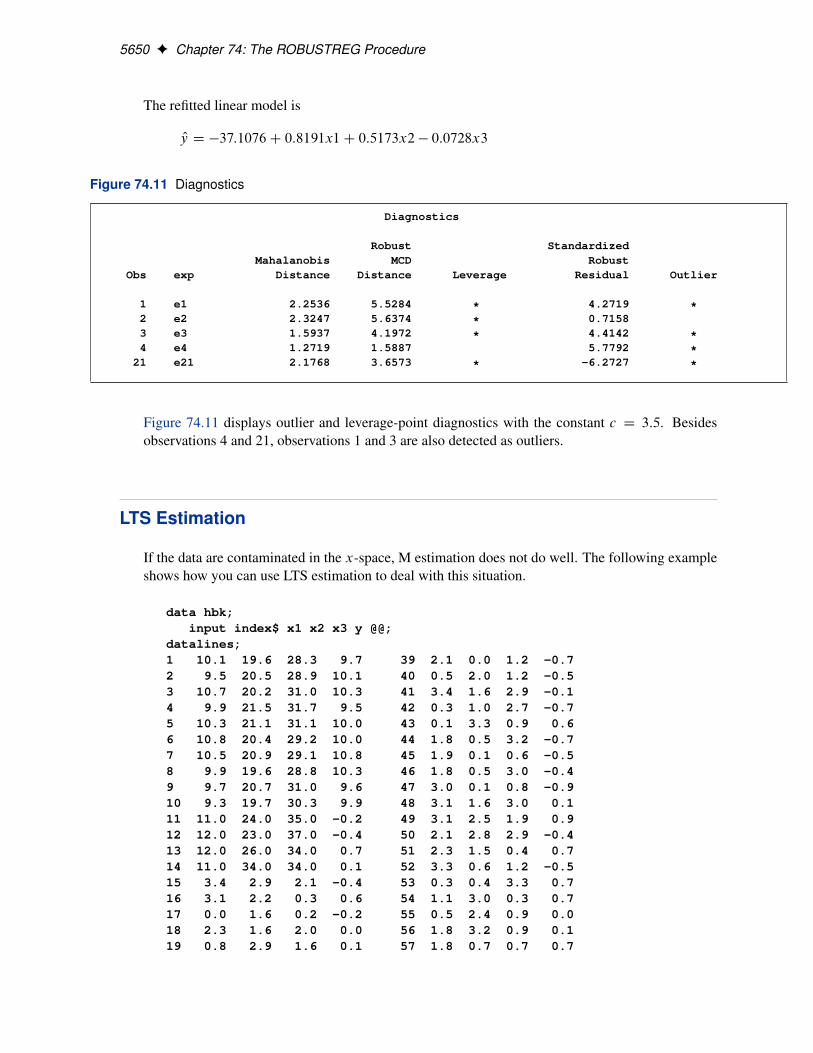
Figure 74.10 Model Parameter Estimates
The ROBUSTREG Procedure
Parameter Estimates
Standard 95% Confidence Chi-Parameter DF Estimate Error Limits Square Pr > ChiSq
Intercept 1 -37.1076 5.4731 -47.8346 -26.3805 45.97 <.0001x1 1 0.8191 0.0620 0.6975 0.9407 174.28 <.0001x2 1 0.5173 0.1693 0.1855 0.8492 9.33 0.0022x3 1 -0.0728 0.0719 -0.2138 0.0681 1.03 0.3111Scale 1 1.4265
Figure 74.10 displays the table of robust parameter estimates, standard errors, and confidence limitswith the constant c D 3:5.
5650 F Chapter 74: The ROBUSTREG Procedure
The refitted linear model is
Oy D �37:1076C 0:8191x1C 0:5173x2 � 0:0728x3
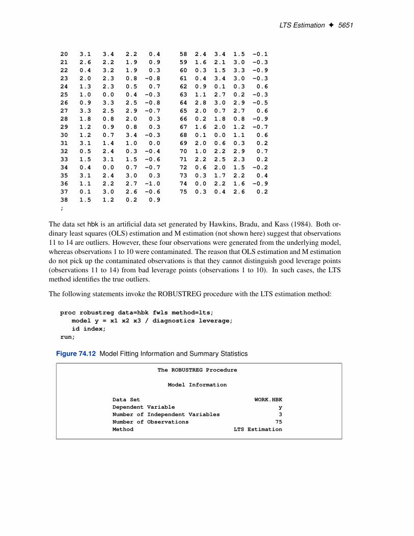
Figure 74.11 Diagnostics
Diagnostics
Robust StandardizedMahalanobis MCD Robust
Obs exp Distance Distance Leverage Residual Outlier
1 e1 2.2536 5.5284 * 4.2719 *2 e2 2.3247 5.6374 * 0.71583 e3 1.5937 4.1972 * 4.4142 *4 e4 1.2719 1.5887 5.7792 *
21 e21 2.1768 3.6573 * -6.2727 *
Figure 74.11 displays outlier and leverage-point diagnostics with the constant c D 3:5. Besidesobservations 4 and 21, observations 1 and 3 are also detected as outliers.
LTS Estimation
If the data are contaminated in the x-space, M estimation does not do well. The following exampleshows how you can use LTS estimation to deal with this situation.
data hbk;input index$ x1 x2 x3 y @@;
datalines;1 10.1 19.6 28.3 9.7 39 2.1 0.0 1.2 -0.72 9.5 20.5 28.9 10.1 40 0.5 2.0 1.2 -0.53 10.7 20.2 31.0 10.3 41 3.4 1.6 2.9 -0.14 9.9 21.5 31.7 9.5 42 0.3 1.0 2.7 -0.75 10.3 21.1 31.1 10.0 43 0.1 3.3 0.9 0.66 10.8 20.4 29.2 10.0 44 1.8 0.5 3.2 -0.77 10.5 20.9 29.1 10.8 45 1.9 0.1 0.6 -0.58 9.9 19.6 28.8 10.3 46 1.8 0.5 3.0 -0.49 9.7 20.7 31.0 9.6 47 3.0 0.1 0.8 -0.910 9.3 19.7 30.3 9.9 48 3.1 1.6 3.0 0.111 11.0 24.0 35.0 -0.2 49 3.1 2.5 1.9 0.912 12.0 23.0 37.0 -0.4 50 2.1 2.8 2.9 -0.413 12.0 26.0 34.0 0.7 51 2.3 1.5 0.4 0.714 11.0 34.0 34.0 0.1 52 3.3 0.6 1.2 -0.515 3.4 2.9 2.1 -0.4 53 0.3 0.4 3.3 0.716 3.1 2.2 0.3 0.6 54 1.1 3.0 0.3 0.717 0.0 1.6 0.2 -0.2 55 0.5 2.4 0.9 0.018 2.3 1.6 2.0 0.0 56 1.8 3.2 0.9 0.119 0.8 2.9 1.6 0.1 57 1.8 0.7 0.7 0.7
LTS Estimation F 5651
20 3.1 3.4 2.2 0.4 58 2.4 3.4 1.5 -0.121 2.6 2.2 1.9 0.9 59 1.6 2.1 3.0 -0.322 0.4 3.2 1.9 0.3 60 0.3 1.5 3.3 -0.923 2.0 2.3 0.8 -0.8 61 0.4 3.4 3.0 -0.324 1.3 2.3 0.5 0.7 62 0.9 0.1 0.3 0.625 1.0 0.0 0.4 -0.3 63 1.1 2.7 0.2 -0.326 0.9 3.3 2.5 -0.8 64 2.8 3.0 2.9 -0.527 3.3 2.5 2.9 -0.7 65 2.0 0.7 2.7 0.628 1.8 0.8 2.0 0.3 66 0.2 1.8 0.8 -0.929 1.2 0.9 0.8 0.3 67 1.6 2.0 1.2 -0.730 1.2 0.7 3.4 -0.3 68 0.1 0.0 1.1 0.631 3.1 1.4 1.0 0.0 69 2.0 0.6 0.3 0.232 0.5 2.4 0.3 -0.4 70 1.0 2.2 2.9 0.733 1.5 3.1 1.5 -0.6 71 2.2 2.5 2.3 0.234 0.4 0.0 0.7 -0.7 72 0.6 2.0 1.5 -0.235 3.1 2.4 3.0 0.3 73 0.3 1.7 2.2 0.436 1.1 2.2 2.7 -1.0 74 0.0 2.2 1.6 -0.937 0.1 3.0 2.6 -0.6 75 0.3 0.4 2.6 0.238 1.5 1.2 0.2 0.9;
The data set hbk is an artificial data set generated by Hawkins, Bradu, and Kass (1984). Both or-dinary least squares (OLS) estimation and M estimation (not shown here) suggest that observations11 to 14 are outliers. However, these four observations were generated from the underlying model,whereas observations 1 to 10 were contaminated. The reason that OLS estimation and M estimationdo not pick up the contaminated observations is that they cannot distinguish good leverage points(observations 11 to 14) from bad leverage points (observations 1 to 10). In such cases, the LTSmethod identifies the true outliers.
The following statements invoke the ROBUSTREG procedure with the LTS estimation method:
proc robustreg data=hbk fwls method=lts;model y = x1 x2 x3 / diagnostics leverage;id index;
run;
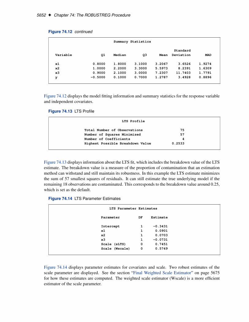
Figure 74.12 Model Fitting Information and Summary Statistics
The ROBUSTREG Procedure
Model Information
Data Set WORK.HBKDependent Variable yNumber of Independent Variables 3Number of Observations 75Method LTS Estimation
5652 F Chapter 74: The ROBUSTREG Procedure
Figure 74.12 continued
Summary Statistics
StandardVariable Q1 Median Q3 Mean Deviation MAD
x1 0.8000 1.8000 3.1000 3.2067 3.6526 1.9274x2 1.0000 2.2000 3.3000 5.5973 8.2391 1.6309x3 0.9000 2.1000 3.0000 7.2307 11.7403 1.7791y -0.5000 0.1000 0.7000 1.2787 3.4928 0.8896
Figure 74.12 displays the model fitting information and summary statistics for the response variableand independent covariates.
Figure 74.13 LTS Profile
LTS Profile
Total Number of Observations 75Number of Squares Minimized 57Number of Coefficients 4Highest Possible Breakdown Value 0.2533
Figure 74.13 displays information about the LTS fit, which includes the breakdown value of the LTSestimate. The breakdown value is a measure of the proportion of contamination that an estimationmethod can withstand and still maintain its robustness. In this example the LTS estimate minimizesthe sum of 57 smallest squares of residuals. It can still estimate the true underlying model if theremaining 18 observations are contaminated. This corresponds to the breakdown value around 0.25,which is set as the default.
Figure 74.14 LTS Parameter Estimates
LTS Parameter Estimates
Parameter DF Estimate
Intercept 1 -0.3431x1 1 0.0901x2 1 0.0703x3 1 -0.0731Scale (sLTS) 0 0.7451Scale (Wscale) 0 0.5749
Figure 74.14 displays parameter estimates for covariates and scale. Two robust estimates of thescale parameter are displayed. See the section “Final Weighted Scale Estimator” on page 5675for how these estimates are computed. The weighted scale estimator (Wscale) is a more efficientestimator of the scale parameter.
LTS Estimation F 5653
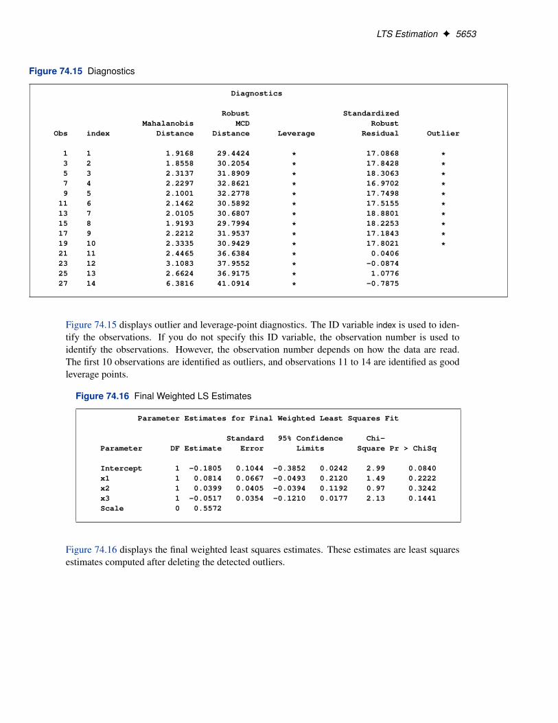
Figure 74.15 Diagnostics
Diagnostics
Robust StandardizedMahalanobis MCD Robust
Obs index Distance Distance Leverage Residual Outlier
1 1 1.9168 29.4424 * 17.0868 *3 2 1.8558 30.2054 * 17.8428 *5 3 2.3137 31.8909 * 18.3063 *7 4 2.2297 32.8621 * 16.9702 *9 5 2.1001 32.2778 * 17.7498 *
11 6 2.1462 30.5892 * 17.5155 *13 7 2.0105 30.6807 * 18.8801 *15 8 1.9193 29.7994 * 18.2253 *17 9 2.2212 31.9537 * 17.1843 *19 10 2.3335 30.9429 * 17.8021 *21 11 2.4465 36.6384 * 0.040623 12 3.1083 37.9552 * -0.087425 13 2.6624 36.9175 * 1.077627 14 6.3816 41.0914 * -0.7875
Figure 74.15 displays outlier and leverage-point diagnostics. The ID variable index is used to iden-tify the observations. If you do not specify this ID variable, the observation number is used toidentify the observations. However, the observation number depends on how the data are read.The first 10 observations are identified as outliers, and observations 11 to 14 are identified as goodleverage points.
Figure 74.16 Final Weighted LS Estimates
Parameter Estimates for Final Weighted Least Squares Fit
Standard 95% Confidence Chi-Parameter DF Estimate Error Limits Square Pr > ChiSq
Intercept 1 -0.1805 0.1044 -0.3852 0.0242 2.99 0.0840x1 1 0.0814 0.0667 -0.0493 0.2120 1.49 0.2222x2 1 0.0399 0.0405 -0.0394 0.1192 0.97 0.3242x3 1 -0.0517 0.0354 -0.1210 0.0177 2.13 0.1441Scale 0 0.5572
Figure 74.16 displays the final weighted least squares estimates. These estimates are least squaresestimates computed after deleting the detected outliers.
5654 F Chapter 74: The ROBUSTREG Procedure
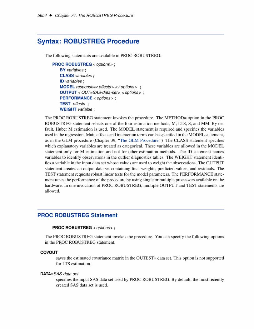
Syntax: ROBUSTREG Procedure
The following statements are available in PROC ROBUSTREG:
PROC ROBUSTREG < options > ;BY variables ;CLASS variables ;ID variables ;MODEL response=< effects > < / options > ;OUTPUT < OUT=SAS-data-set > < options > ;PERFORMANCE < options > ;TEST effects ;WEIGHT variable ;
The PROC ROBUSTREG statement invokes the procedure. The METHOD= option in the PROCROBUSTREG statement selects one of the four estimation methods, M, LTS, S, and MM. By de-fault, Huber M estimation is used. The MODEL statement is required and specifies the variablesused in the regression. Main effects and interaction terms can be specified in the MODEL statement,as in the GLM procedure (Chapter 39, “The GLM Procedure.”) The CLASS statement specifieswhich explanatory variables are treated as categorical. These variables are allowed in the MODELstatement only for M estimation and not for other estimation methods. The ID statement namesvariables to identify observations in the outlier diagnostics tables. The WEIGHT statement identi-fies a variable in the input data set whose values are used to weight the observations. The OUTPUTstatement creates an output data set containing final weights, predicted values, and residuals. TheTEST statement requests robust linear tests for the model parameters. The PERFORMANCE state-ment tunes the performance of the procedure by using single or multiple processors available on thehardware. In one invocation of PROC ROBUSTREG, multiple OUTPUT and TEST statements areallowed.
PROC ROBUSTREG Statement
PROC ROBUSTREG < options > ;
The PROC ROBUSTREG statement invokes the procedure. You can specify the following optionsin the PROC ROBUSTREG statement.
COVOUTsaves the estimated covariance matrix in the OUTEST= data set. This option is not supportedfor LTS estimation.
DATA=SAS-data-setspecifies the input SAS data set used by PROC ROBUSTREG. By default, the most recentlycreated SAS data set is used.
PROC ROBUSTREG Statement F 5655
FWLSrequests that final weighted least squares estimates be computed. These estimates are equiv-alent to the least squares estimates after the detected outliers are deleted.
INEST=SAS-data-setspecifies an input SAS data set that contains initial estimates for all the parameters in themodel. See the section “INEST= Data Set” on page 5683 for a detailed description of thecontents of the INEST= data set.
ITPRINTdisplays the iteration history for the iteratively reweighted least squares algorithm used by Mand MM estimation. You can also use this option in the MODEL statement.
NAMELEN=nspecifies the length of effect names in tables and output data sets to be n characters, where nis a value between 20 and 200. The default length is 20 characters.
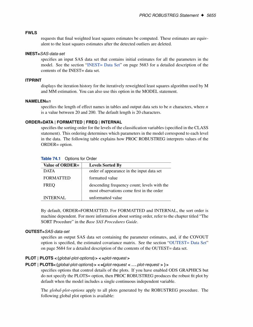
ORDER=DATA | FORMATTED | FREQ | INTERNALspecifies the sorting order for the levels of the classification variables (specified in the CLASSstatement). This ordering determines which parameters in the model correspond to each levelin the data. The following table explains how PROC ROBUSTREG interprets values of theORDER= option.
Table 74.1 Options for Order
Value of ORDER= Levels Sorted ByDATA order of appearance in the input data set
FORMATTED formatted value
FREQ descending frequency count; levels with themost observations come first in the order
INTERNAL unformatted value
By default, ORDER=FORMATTED. For FORMATTED and INTERNAL, the sort order ismachine dependent. For more information about sorting order, refer to the chapter titled “TheSORT Procedure” in the Base SAS Procedures Guide.
OUTEST=SAS-data-setspecifies an output SAS data set containing the parameter estimates, and, if the COVOUToption is specified, the estimated covariance matrix. See the section “OUTEST= Data Set”on page 5684 for a detailed description of the contents of the OUTEST= data set.
PLOT | PLOTS < (global-plot-options) > < =plot-request >
PLOT | PLOTS< (global-plot-options) > < =(plot-request < . . . plot-request > ) >specifies options that control details of the plots. If you have enabled ODS GRAPHICS butdo not specify the PLOTS= option, then PROC ROBUSTREG produces the robust fit plot bydefault when the model includes a single continuous independent variable.
The global-plot-options apply to all plots generated by the ROBUSTREG procedure. Thefollowing global plot option is available:
5656 F Chapter 74: The ROBUSTREG Procedure
ONLYsuppresses the default robust fit plot. Only plots specifically requested are displayed.
You can specify more than one plot request within the parentheses after PLOTS=. For a singleplot request, you can omit the parentheses. The following plot requests are available.
ALLcreates all appropriate plots.
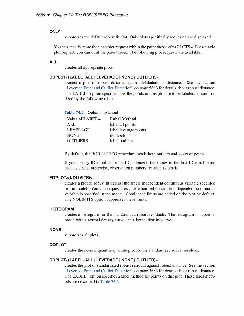
DDPLOT<(LABEL=ALL | LEVERAGE | NONE | OUTLIER)>creates a plot of robust distance against Mahalanobis distance. See the section“Leverage Point and Outlier Detection” on page 5683 for details about robust distance.The LABEL= option specifies how the points on this plot are to be labeled, as summa-rized by the following table.
Table 74.2 Options for Label
Value of LABEL= Label MethodALL label all pointsLEVERAGE label leverage pointsNONE no labelsOUTLIERS label outliers
By default, the ROBUSTREG procedure labels both outliers and leverage points.
If you specify ID variables in the ID statement, the values of the first ID variable areused as labels; otherwise, observation numbers are used as labels.
FITPLOT<(NOLIMITS)>creates a plot of robust fit against the single independent continuous variable specifiedin the model. You can request this plot when only a single independent continuousvariable is specified in the model. Confidence limits are added on the plot by default.The NOLIMITS option suppresses these limits.
HISTOGRAMcreates a histogram for the standardized robust residuals. The histogram is superim-posed with a normal density curve and a kernel density curve.
NONEsuppresses all plots.
QQPLOTcreates the normal quantile-quantile plot for the standardized robust residuals.
RDPLOT<(LABEL=ALL | LEVERAGE | NONE | OUTLIER)>creates the plot of standardized robust residual against robust distance. See the section“Leverage Point and Outlier Detection” on page 5683 for details about robust distance.The LABEL= option specifies a label method for points on this plot. These label meth-ods are described in Table 74.2.
PROC ROBUSTREG Statement F 5657
If you specify ID variables in the ID statement, the values of the first ID variable areused as labels; otherwise, observation numbers are used as labels.
SEED=numberspecifies the seed for the random number generator used to randomly select the subgroupsand subsets for LTS and S estimation. By default or if you specify zero, the ROBUSTREGprocedure generates a random seed.
METHOD=method type < ( options ) >specifies the estimation method and options specify some additional options for the estima-tion method. PROC ROBUSTREG provides four estimation methods: M estimation, LTSestimation, S estimation, and MM estimation. The default method is M estimation.
NOTE: Since the LTS and S methods use subsampling algorithms, these methods are not suit-able in an analysis with categorical independent variables specified in the CLASS statement.These methods are not suitable in an analysis with continuous independent variables that haveonly a few unequal values or a few unequal values within one BY group. This also applies tothe initial LTS and S estimates in the MM method. In summary, if the model includes cate-gorical independent variables or continuous independent variables with a few unequal values,the M method is recommended.
Options with METHOD=M
With METHOD=M, you can specify the following additional options:
ASYMPCOV=H1 | H2 | H3specifies the type of asymptotic covariance computed for the M estimate. The threetypes are described in the section “Asymptotic Covariance and Confidence Intervals”on page 5671. By default, ASYMPCOV= H1.
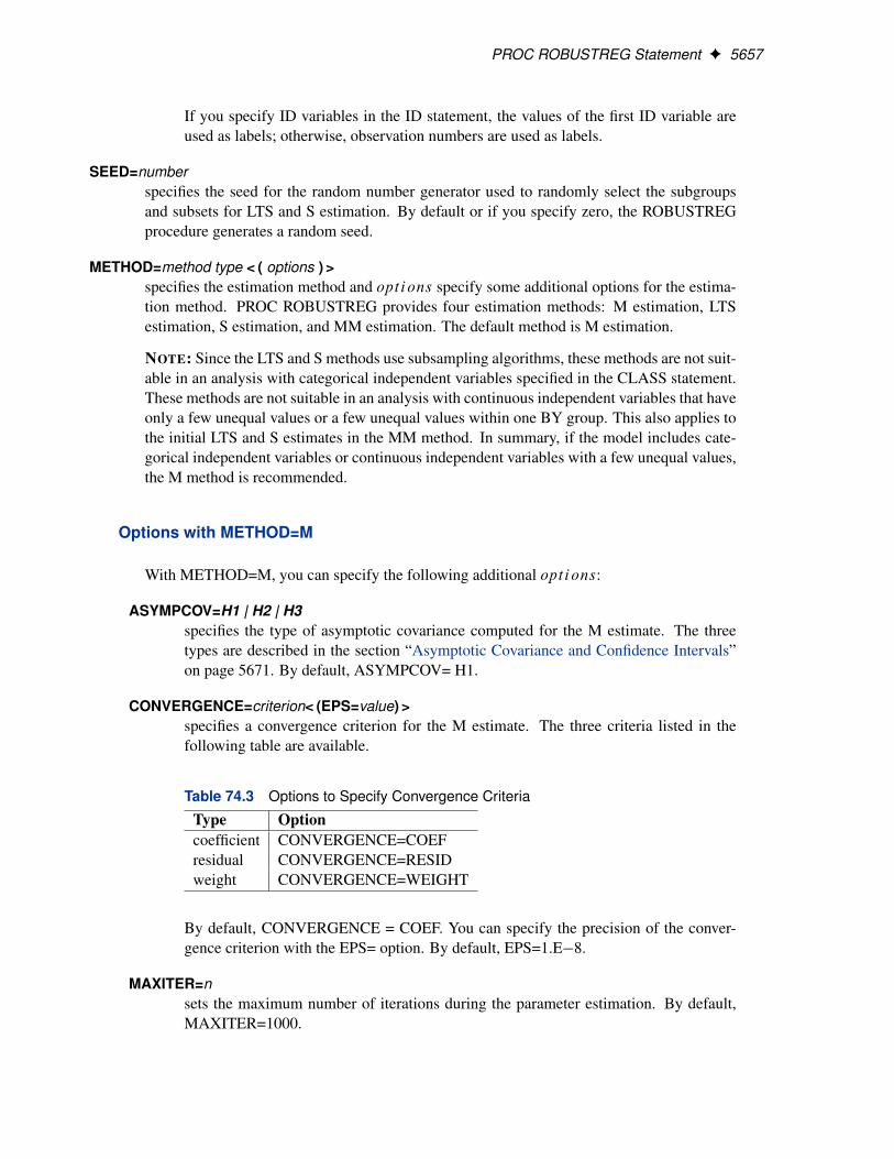
CONVERGENCE=criterion< (EPS=value) >specifies a convergence criterion for the M estimate. The three criteria listed in thefollowing table are available.
Table 74.3 Options to Specify Convergence Criteria
Type Optioncoefficient CONVERGENCE=COEFresidual CONVERGENCE=RESIDweight CONVERGENCE=WEIGHT
By default, CONVERGENCE = COEF. You can specify the precision of the conver-gence criterion with the EPS= option. By default, EPS=1.E�8.
MAXITER=nsets the maximum number of iterations during the parameter estimation. By default,MAXITER=1000.
5658 F Chapter 74: The ROBUSTREG Procedure
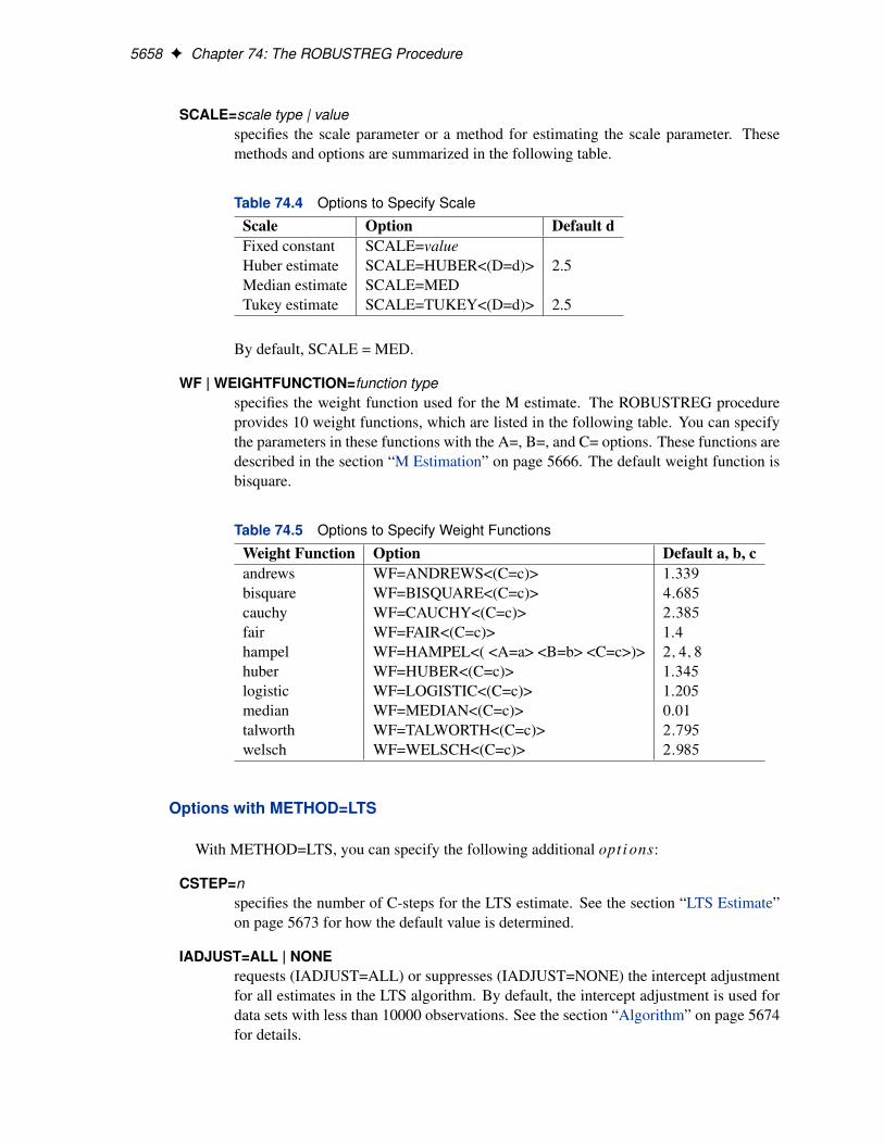
SCALE=scale type | valuespecifies the scale parameter or a method for estimating the scale parameter. Thesemethods and options are summarized in the following table.
Table 74.4 Options to Specify Scale
Scale Option Default dFixed constant SCALE=valueHuber estimate SCALE=HUBER<(D=d)> 2.5Median estimate SCALE=MEDTukey estimate SCALE=TUKEY<(D=d)> 2.5
By default, SCALE = MED.
WF | WEIGHTFUNCTION=function typespecifies the weight function used for the M estimate. The ROBUSTREG procedureprovides 10 weight functions, which are listed in the following table. You can specifythe parameters in these functions with the A=, B=, and C= options. These functions aredescribed in the section “M Estimation” on page 5666. The default weight function isbisquare.
Table 74.5 Options to Specify Weight Functions
Weight Function Option Default a, b, candrews WF=ANDREWS<(C=c)> 1:339
bisquare WF=BISQUARE<(C=c)> 4:685
cauchy WF=CAUCHY<(C=c)> 2:385
fair WF=FAIR<(C=c)> 1:4
hampel WF=HAMPEL<( <A=a> <B=b> <C=c>)> 2; 4; 8
huber WF=HUBER<(C=c)> 1:345
logistic WF=LOGISTIC<(C=c)> 1:205
median WF=MEDIAN<(C=c)> 0:01
talworth WF=TALWORTH<(C=c)> 2:795
welsch WF=WELSCH<(C=c)> 2:985
Options with METHOD=LTS
With METHOD=LTS, you can specify the following additional options:
CSTEP=nspecifies the number of C-steps for the LTS estimate. See the section “LTS Estimate”on page 5673 for how the default value is determined.
IADJUST=ALL | NONErequests (IADJUST=ALL) or suppresses (IADJUST=NONE) the intercept adjustmentfor all estimates in the LTS algorithm. By default, the intercept adjustment is used fordata sets with less than 10000 observations. See the section “Algorithm” on page 5674for details.
PROC ROBUSTREG Statement F 5659
H=nspecifies the quantile for the LTS estimate. See the section “LTS Estimate” onpage 5673 for how the default value is determined.
NBEST=nspecifies the number of best solutions kept for each subgroup during the computationof the LTS estimate. The default number is 10, which is the maximum number allowed.
NREP=nspecifies the number of repeats of least squares fit in subgroups during the computationof the LTS estimate. See the section “LTS Estimate” on page 5673 for how the defaultnumber is determined.
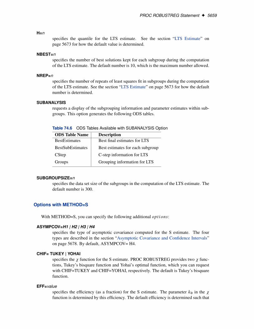
SUBANALYSISrequests a display of the subgrouping information and parameter estimates within sub-groups. This option generates the following ODS tables.
Table 74.6 ODS Tables Available with SUBANALYSIS Option
ODS Table Name DescriptionBestEstimates Best final estimates for LTS
BestSubEstimates Best estimates for each subgroup
CStep C-step information for LTS
Groups Grouping information for LTS
SUBGROUPSIZE=nspecifies the data set size of the subgroups in the computation of the LTS estimate. Thedefault number is 300.
Options with METHOD=S
With METHOD=S, you can specify the following additional options:
ASYMPCOV=H1 | H2 | H3 | H4specifies the type of asymptotic covariance computed for the S estimate. The fourtypes are described in the section “Asymptotic Covariance and Confidence Intervals”on page 5678. By default, ASYMPCOV= H4.
CHIF= TUKEY | YOHAIspecifies the � function for the S estimate. PROC ROBUSTREG provides two � func-tions, Tukey’s bisquare function and Yohai’s optimal function, which you can requestwith CHIF=TUKEY and CHIF=YOHAI, respectively. The default is Tukey’s bisquarefunction.
EFF=valuespecifies the efficiency (as a fraction) for the S estimate. The parameter k0 in the �function is determined by this efficiency. The default efficiency is determined such that
5660 F Chapter 74: The ROBUSTREG Procedure
the consistent S estimate has the breakdown value of 25%. This option is overwrittenby the K0= option if both of them are used.
K0=valuespecifies the k0 parameter in the � function of the S estimate. For CHIF=TUKEY,the default is 1.548. For CHIF=YOHAI, the default is 0.66. These default valuescorrespond to a 50% breakdown value of the consistent S estimate.
MAXITER=nsets the maximum number of iterations for computing the scale parameter of the Sestimate. By default, MAXITER=1000.
NREP=nspecifies the number of repeats of subsampling in the computation of the S estimate.See the section “Algorithm” on page 5676 for how the default number of repeats isdetermined.
NOREFINEsuppresses the refinement for the S estimate. See the section “Algorithm” on page 5676for details.
SUBSETSIZE=nspecifies the size of the subset for the S estimate. See the section “Algorithm” onpage 5676 for how its default value is determined.
TOLERANCE=valuespecifies the tolerance for the S estimate of the scale. The default value is 0.001.
Options with METHOD=MM
With METHOD=MM, you can specify the following additional options:
ASYMPCOV=H1 | H2 | H3 | H4specifies the type of asymptotic covariance computed for the MM estimate. The fourtypes are described in the section “Details: ROBUSTREG Procedure” on page 5666.By default, ASYMPCOV= H4.
BIASTEST< (ALPHA=number ) >requests the bias test for the final MM estimate. See the section “Bias Test” onpage 5680 for details about this test.
CHIF= TUKEY | YOHAIselects the � function for the MM estimate. PROC ROBUSTREG provides two �functions: Tukey’s bisquare function and Yohai’s optimal function, which you can re-quest with CHIF=TUKEY and CHIF=YOHAI, respectively. The default is Tukey’sbisquare function. This � function is also used by the initial S estimate if you specifythe INITEST=S option.
BY Statement F 5661
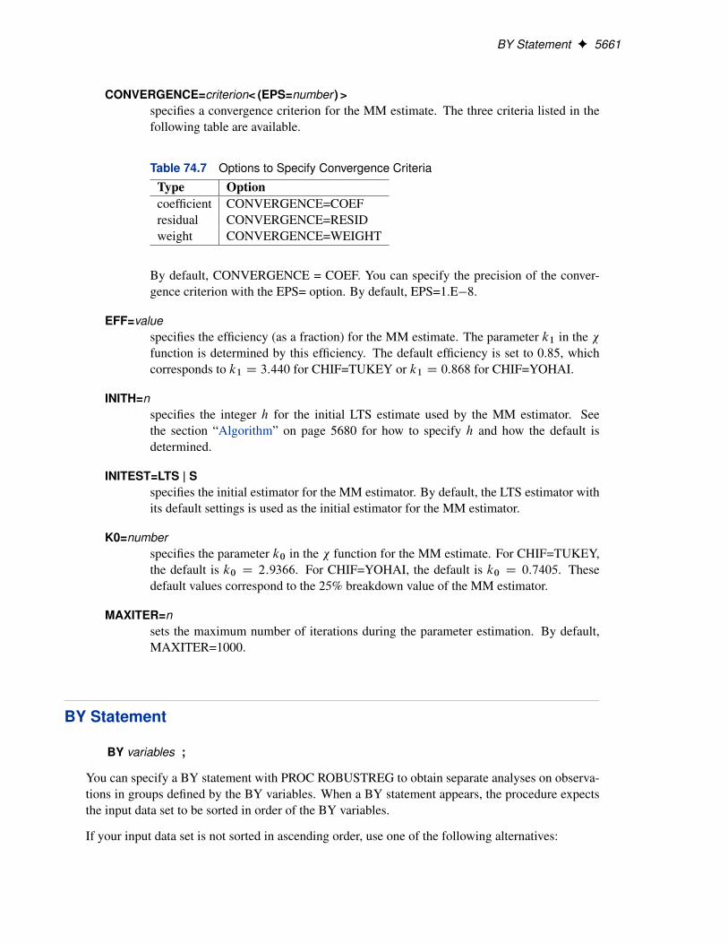
CONVERGENCE=criterion< (EPS=number ) >specifies a convergence criterion for the MM estimate. The three criteria listed in thefollowing table are available.
Table 74.7 Options to Specify Convergence Criteria
Type Optioncoefficient CONVERGENCE=COEFresidual CONVERGENCE=RESIDweight CONVERGENCE=WEIGHT
By default, CONVERGENCE = COEF. You can specify the precision of the conver-gence criterion with the EPS= option. By default, EPS=1.E�8.
EFF=valuespecifies the efficiency (as a fraction) for the MM estimate. The parameter k1 in the �function is determined by this efficiency. The default efficiency is set to 0.85, whichcorresponds to k1 D 3:440 for CHIF=TUKEY or k1 D 0:868 for CHIF=YOHAI.
INITH=nspecifies the integer h for the initial LTS estimate used by the MM estimator. Seethe section “Algorithm” on page 5680 for how to specify h and how the default isdetermined.
INITEST=LTS | Sspecifies the initial estimator for the MM estimator. By default, the LTS estimator withits default settings is used as the initial estimator for the MM estimator.
K0=numberspecifies the parameter k0 in the � function for the MM estimate. For CHIF=TUKEY,the default is k0 D 2:9366. For CHIF=YOHAI, the default is k0 D 0:7405. Thesedefault values correspond to the 25% breakdown value of the MM estimator.
MAXITER=nsets the maximum number of iterations during the parameter estimation. By default,MAXITER=1000.
BY Statement
BY variables ;
You can specify a BY statement with PROC ROBUSTREG to obtain separate analyses on observa-tions in groups defined by the BY variables. When a BY statement appears, the procedure expectsthe input data set to be sorted in order of the BY variables.
If your input data set is not sorted in ascending order, use one of the following alternatives:
5662 F Chapter 74: The ROBUSTREG Procedure
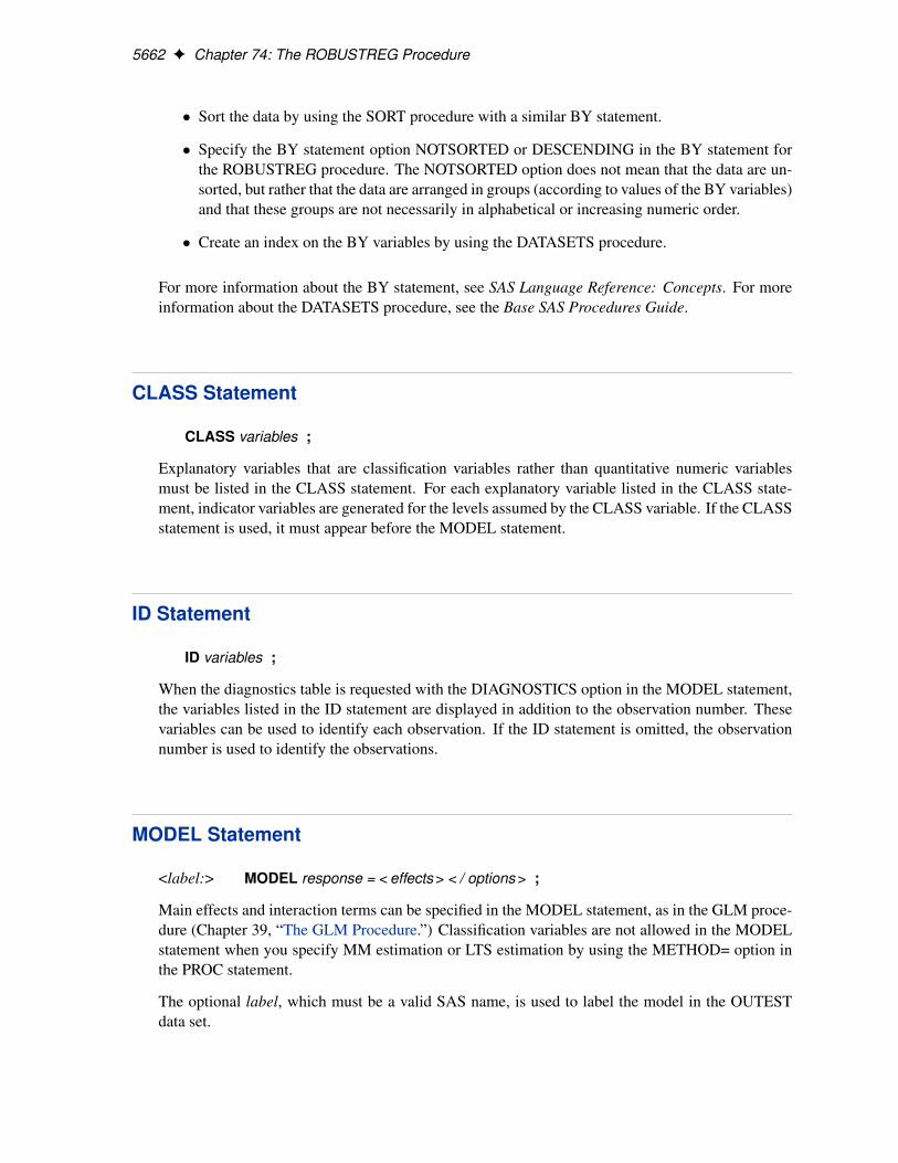
� Sort the data by using the SORT procedure with a similar BY statement.
� Specify the BY statement option NOTSORTED or DESCENDING in the BY statement forthe ROBUSTREG procedure. The NOTSORTED option does not mean that the data are un-sorted, but rather that the data are arranged in groups (according to values of the BY variables)and that these groups are not necessarily in alphabetical or increasing numeric order.
� Create an index on the BY variables by using the DATASETS procedure.
For more information about the BY statement, see SAS Language Reference: Concepts. For moreinformation about the DATASETS procedure, see the Base SAS Procedures Guide.
CLASS Statement
CLASS variables ;
Explanatory variables that are classification variables rather than quantitative numeric variablesmust be listed in the CLASS statement. For each explanatory variable listed in the CLASS state-ment, indicator variables are generated for the levels assumed by the CLASS variable. If the CLASSstatement is used, it must appear before the MODEL statement.
ID Statement
ID variables ;
When the diagnostics table is requested with the DIAGNOSTICS option in the MODEL statement,the variables listed in the ID statement are displayed in addition to the observation number. Thesevariables can be used to identify each observation. If the ID statement is omitted, the observationnumber is used to identify the observations.
MODEL Statement
<label:> MODEL response = < effects > < / options > ;
Main effects and interaction terms can be specified in the MODEL statement, as in the GLM proce-dure (Chapter 39, “The GLM Procedure.”) Classification variables are not allowed in the MODELstatement when you specify MM estimation or LTS estimation by using the METHOD= option inthe PROC statement.
The optional label, which must be a valid SAS name, is used to label the model in the OUTESTdata set.
MODEL Statement F 5663
You can specify the following options for the model fit.
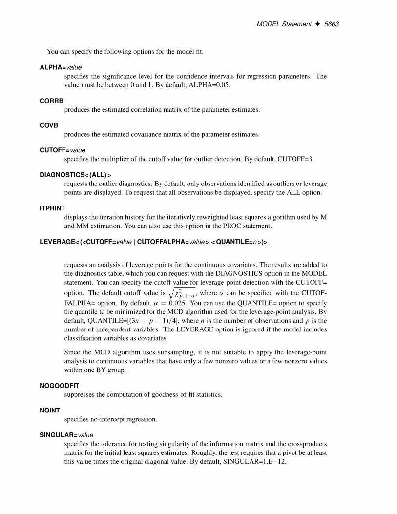
ALPHA=valuespecifies the significance level for the confidence intervals for regression parameters. Thevalue must be between 0 and 1. By default, ALPHA=0.05.
CORRBproduces the estimated correlation matrix of the parameter estimates.
COVBproduces the estimated covariance matrix of the parameter estimates.
CUTOFF=valuespecifies the multiplier of the cutoff value for outlier detection. By default, CUTOFF=3.
DIAGNOSTICS< (ALL) >requests the outlier diagnostics. By default, only observations identified as outliers or leveragepoints are displayed. To request that all observations be displayed, specify the ALL option.
ITPRINTdisplays the iteration history for the iteratively reweighted least squares algorithm used by Mand MM estimation. You can also use this option in the PROC statement.
LEVERAGE< (<CUTOFF=value | CUTOFFALPHA=value > < QUANTILE=n >)>
requests an analysis of leverage points for the continuous covariates. The results are added tothe diagnostics table, which you can request with the DIAGNOSTICS option in the MODELstatement. You can specify the cutoff value for leverage-point detection with the CUTOFF=
option. The default cutoff value isq�2pI1�˛, where ˛ can be specified with the CUTOF-
FALPHA= option. By default, ˛ D 0:025. You can use the QUANTILE= option to specifythe quantile to be minimized for the MCD algorithm used for the leverage-point analysis. Bydefault, QUANTILE=Œ.3nC p C 1/=4�, where n is the number of observations and p is thenumber of independent variables. The LEVERAGE option is ignored if the model includesclassification variables as covariates.
Since the MCD algorithm uses subsampling, it is not suitable to apply the leverage-pointanalysis to continuous variables that have only a few nonzero values or a few nonzero valueswithin one BY group.
NOGOODFITsuppresses the computation of goodness-of-fit statistics.
NOINTspecifies no-intercept regression.
SINGULAR=valuespecifies the tolerance for testing singularity of the information matrix and the crossproductsmatrix for the initial least squares estimates. Roughly, the test requires that a pivot be at leastthis value times the original diagonal value. By default, SINGULAR=1.E�12.
5664 F Chapter 74: The ROBUSTREG Procedure
OUTPUT Statement
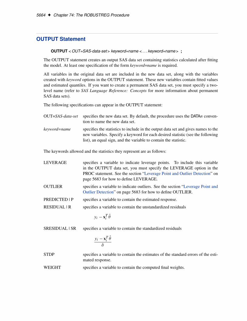
OUTPUT < OUT=SAS-data-set > keyword=name < . . . keyword=name > ;
The OUTPUT statement creates an output SAS data set containing statistics calculated after fittingthe model. At least one specification of the form keyword=name is required.
All variables in the original data set are included in the new data set, along with the variablescreated with keyword options in the OUTPUT statement. These new variables contain fitted valuesand estimated quantiles. If you want to create a permanent SAS data set, you must specify a two-level name (refer to SAS Language Reference: Concepts for more information about permanentSAS data sets).
The following specifications can appear in the OUTPUT statement:
OUT=SAS-data-set specifies the new data set. By default, the procedure uses the DATAn conven-tion to name the new data set.
keyword=name specifies the statistics to include in the output data set and gives names to thenew variables. Specify a keyword for each desired statistic (see the followinglist), an equal sign, and the variable to contain the statistic.
The keywords allowed and the statistics they represent are as follows:
LEVERAGE specifies a variable to indicate leverage points. To include this variablein the OUTPUT data set, you must specify the LEVERAGE option in thePROC statement. See the section “Leverage Point and Outlier Detection” onpage 5683 for how to define LEVERAGE.
OUTLIER specifies a variable to indicate outliers. See the section “Leverage Point andOutlier Detection” on page 5683 for how to define OUTLIER.
PREDICTED | P specifies a variable to contain the estimated response.
RESIDUAL | R specifies a variable to contain the unstandardized residuals
yi � xTi O�
SRESIDUAL | SR specifies a variable to contain the standardized residuals
yi � xTi O�
O�
STDP specifies a variable to contain the estimates of the standard errors of the esti-mated response.
WEIGHT specifies a variable to contain the computed final weights.
PERFORMANCE Statement F 5665
PERFORMANCE Statement
The PERFORMANCE statement is used to change default options that affect the performance ofPROC ROBUSTREG and to request tables that show the performance options in effect and timingdetails. See Chen (2002) for some empirical results.
PERFORMANCE < options > ;
The following options are available:
CPUCOUNT=1-1024
CPUCOUNT=ACTUALspecifies the number of processors to use for forming crossproduct matrices. CPU-COUNT=ACTUAL sets CPUCOUNT to be the number of physical processors available.Note that this can be less than the physical number of CPUs if the SAS process has beenrestricted by system administration tools. Setting CPUCOUNT= to a number greater than theactual number of available CPUs might result in reduced performance. This option overridesthe SAS system option CPUCOUNT=. If CPUCOUNT=1, then NOTHREADS is in effect,and PROC ROBUSTREG uses singly threaded code.
DETAILSrequests the “PerfSettings” table that shows the performance settings in effect and the “Tim-ing” table that provides a broad timing breakdown of the PROC ROBUSTREG step.
THREADSenables multithreaded computation. This option overrides the SAS system optionTHREADS | NOTHREADS.
NOTHREADSdisables multithreaded computation. This option overrides the SAS system optionTHREADS | NOTHREADS.
TEST Statement
<label:> TEST effects ;
With M estimation and MM estimation, the TEST statement provides a means of obtaining a testfor the canonical linear hypothesis concerning the parameters of the tested effects:
�j D 0; j D i1; : : : ; iq
where q is the total number of parameters of the tested effects.
PROC ROBUSTREG provides two kinds of robust tests: the � test and the R2n test. They aredescribed in the section “Details: ROBUSTREG Procedure” on page 5666. No test is available forLTS and S estimation.
5666 F Chapter 74: The ROBUSTREG Procedure
The optional label, which must be a valid SAS name, is used to label output from the correspondingTEST statement.
WEIGHT Statement
WEIGHT variable ;
The WEIGHT statement specifies a weight variable in the input data set.
If you want to use fixed weights for each observation in the input data set, place the weights in avariable in the data set and specify the name in a WEIGHT statement. The values of the WEIGHTvariable can be nonintegral and are not truncated. Observations with nonpositive or missing valuesfor the weight variable do not contribute to the fit of the model.
Details: ROBUSTREG Procedure
This section describes the statistical and computational aspects of the ROBUSTREG procedure.The following notation is used throughout this section.
LetX D .xij / denote an n�p matrix, y D .y1; : : : ; yn/T denote a given n-vector of responses, and
� D .�1; : : : ; �p/T denote an unknown p-vector of parameters or coefficients whose components
are to be estimated. The matrix X is called the design matrix. Consider the usual linear model
y D X� C e
where e D .e1; : : : ; en/T is an n-vector of unknown errors. It is assumed that (for a given X ) the
components ei of e are independent and identically distributed according to a distribution L.�=�/,where � is a scale parameter (usually unknown). Often L.�/ � ˆ.�/, the standard normal distribu-tion function. The vector of residuals for a given value of O� is denoted by r D .r1; : : : ; rn/
T andthe i th row of the matrix X is denoted by xTi .
M Estimation
M estimation in the context of regression was first introduced by Huber (1973) as a result of makingthe least squares approach robust. Although M estimators are not robust with respect to leveragepoints, they are popular in applications where leverage points are not an issue.
Instead of minimizing a sum of squares of the residuals, a Huber-type M estimator O�M of � mini-mizes a sum of less rapidly increasing functions of the residuals:
M Estimation F 5667
Q.�/ D
nXiD1
�.ri
�/
where r D y �X� . For the ordinary least squares estimation, � is the square function, �.z/ D z2.
If � is known, then by taking derivatives with respect to � , O�M is also a solution of the system of pequations:
nXiD1
.ri
�/xij D 0; j D 1; : : : ; p
where D@�@z
. If � is convex, O�M is the unique solution.
The ROBUSTREG procedure solves this system by using iteratively reweighted least squares(IRLS). The weight function w.x/ is defined as
w.z/ D .z/
z
The ROBUSTREG procedure provides 10 kinds of weight functions through the WEIGHTFUNC-TION= option in the MODEL statement. Each weight function corresponds to a � function. Seethe section “Weight Functions” on page 5668 for a complete discussion. You can specify the scaleparameter � with the SCALE= option in the PROC statement.
If � is unknown, both � and � are estimated by minimizing the function
Q.�; �/ D
nXiD1
Œ�.ri
�/C a��; a > 0
The algorithm proceeds by alternately improving O� in a location step and O� in a scale step.
For the scale step, three methods are available to estimate � , which you can select with the SCALE=option.
1. (SCALE=HUBER<(D=d)>) Compute O� by the iteration
. O� .mC1//2 D1
nh
nXiD1
�d .ri
O� .m//. O� .m//2
where
5668 F Chapter 74: The ROBUSTREG Procedure
�d .x/ D
�x2=2 if jxj < d
d2=2 otherwise
is the Huber function and h Dn�pn.d2 C .1� d2/ˆ.d/� 0:5� d
p2�e� 1
2d2
/ is the Huberconstant (refer to Huber 1981, p. 179). You can specify d with the D= option. By default,d D 2:5.
2. (SCALE=TUKEY<(D=d)>) Compute O� by solving the supplementary equation
1
n � p
nXiD1
�d .ri
�/ D ˇ
where
�d .x/ D
(3x2
d2 �3x4
d4 Cx6
d6 if jxj < d
1 otherwise
Here D16�01 is Tukey’s bisquare function, and ˇ D
R�d .s/dˆ.s/ is the constant such
that the solution O� is asymptotically consistent when L.�=�/ D ˆ.�/ (refer to Hampel et al.1986, p. 149). You can specify d with the D= option. By default, d D 2:5.
3. (SCALE=MED) Compute O� by the iteration
O� .mC1/D medianfjyi � xTi
O� .m/j=ˇ0; i D 1; : : : ; ng
where ˇ0 D ˆ�1.:75/ is the constant such that the solution O� is asymptotically consistentwhen L.�=�/ D ˆ.�/ (refer to Hampel et al. 1986, p. 312).
Note that SCALE = MED is the default.
Algorithm
The basic algorithm for computing M estimates for regression is iteratively reweighted least squares(IRLS). As the name suggests, a weighted least squares fit is carried out inside an iteration loop.For each iteration, a set of weights for the observations is used in the least squares fit. The weightsare constructed by applying a weight function to the current residuals. Initial weights are based onresiduals from an initial fit. The ROBUSTREG procedure uses the unweighted least squares fit as adefault initial fit. The iteration terminates when a convergence criterion is satisfied. The maximumnumber of iterations is set to 1000. You can specify the weight function and the convergence criteria.
Weight Functions
You can specify the weight function for M estimation with the WEIGHTFUNCTION= option. TheROBUSTREG procedure provides 10 weight functions. By default, the procedure uses the bisquare
M Estimation F 5669
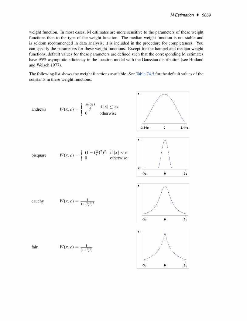
weight function. In most cases, M estimates are more sensitive to the parameters of these weightfunctions than to the type of the weight function. The median weight function is not stable andis seldom recommended in data analysis; it is included in the procedure for completeness. Youcan specify the parameters for these weight functions. Except for the hampel and median weightfunctions, default values for these parameters are defined such that the corresponding M estimateshave 95% asymptotic efficiency in the location model with the Gaussian distribution (see Hollandand Welsch 1977).
The following list shows the weight functions available. See Table 74.5 for the default values of theconstants in these weight functions.
andrews W.x; c/ D
(sin.x
c/
xc
if jxj � �c
0 otherwise
bisquare W.x; c/ D
�.1 � .x
c/2/2 if jxj < c
0 otherwise
cauchy W.x; c/ D1
1C. jxj
c/2
fair W.x; c/ D1
.1Cjxj
c/
5670 F Chapter 74: The ROBUSTREG Procedure
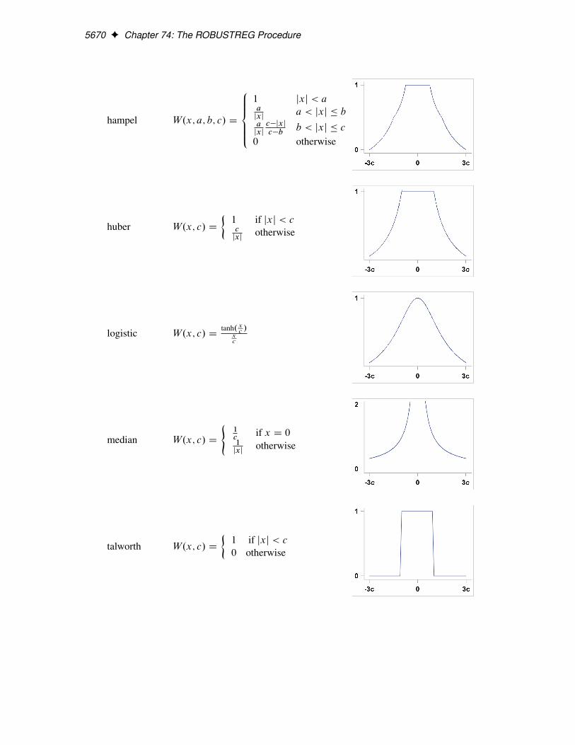
hampel W.x; a; b; c/ D
8̂̂̂<̂ˆ̂:1 jxj < aa
jxja < jxj � b
ajxj
c�jxj
c�bb < jxj � c
0 otherwise
huber W.x; c/ D
�1 if jxj < cc
jxjotherwise
logistic W.x; c/ Dtanh.x
c/
xc
median W.x; c/ D
(1c
if x D 01
jxjotherwise
talworth W.x; c/ D
�1 if jxj < c
0 otherwise
M Estimation F 5671
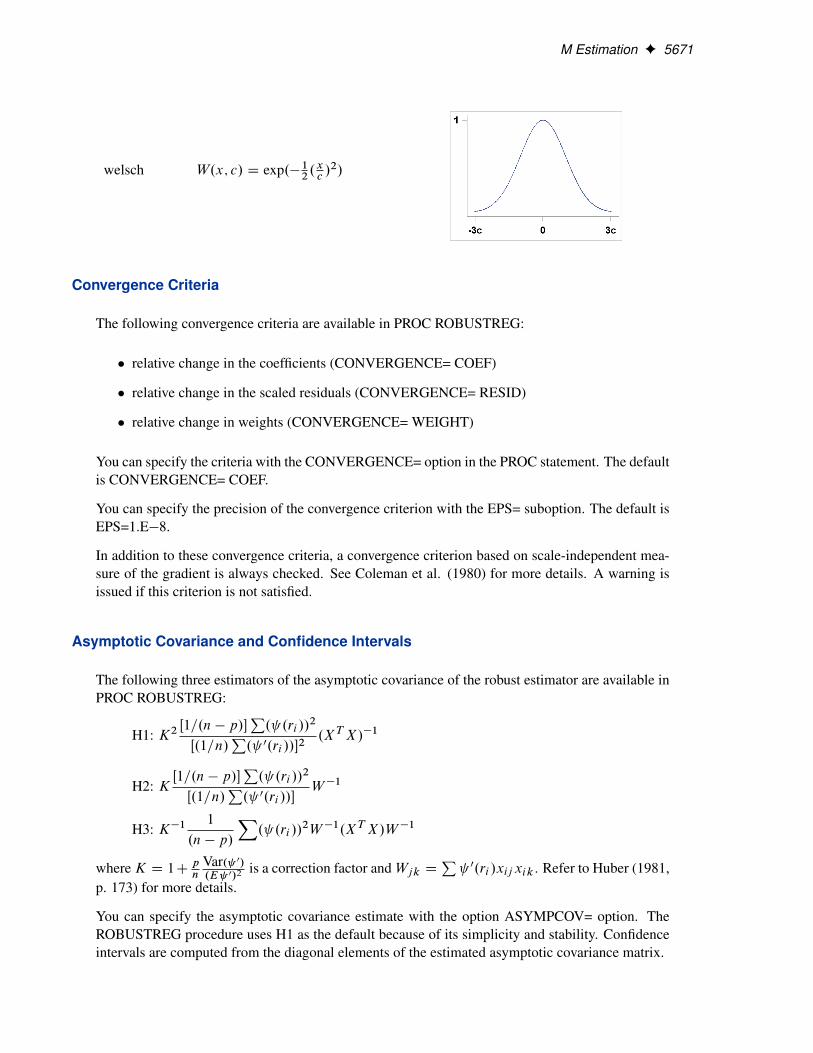
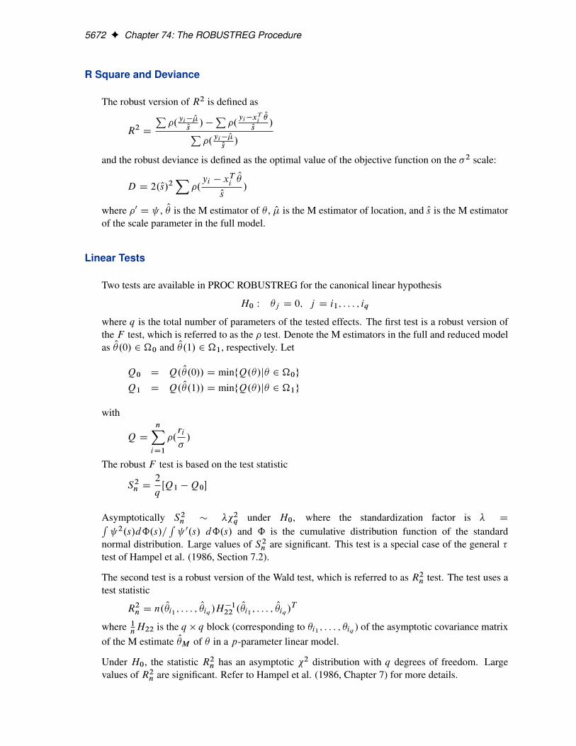
welsch W.x; c/ D exp.�12.xc/2/
Convergence Criteria
The following convergence criteria are available in PROC ROBUSTREG:
� relative change in the coefficients (CONVERGENCE= COEF)
� relative change in the scaled residuals (CONVERGENCE= RESID)
� relative change in weights (CONVERGENCE= WEIGHT)
You can specify the criteria with the CONVERGENCE= option in the PROC statement. The defaultis CONVERGENCE= COEF.
You can specify the precision of the convergence criterion with the EPS= suboption. The default isEPS=1.E�8.
In addition to these convergence criteria, a convergence criterion based on scale-independent mea-sure of the gradient is always checked. See Coleman et al. (1980) for more details. A warning isissued if this criterion is not satisfied.
Asymptotic Covariance and Confidence Intervals
The following three estimators of the asymptotic covariance of the robust estimator are available inPROC ROBUSTREG:
H1: K2Œ1=.n � p/�
P. .ri //
2
Œ.1=n/P. 0.ri //�2
.XTX/�1
H2: KŒ1=.n � p/�
P. .ri //
2
Œ.1=n/P. 0.ri //�
W �1
H3: K�1 1
.n � p/
X. .ri //
2W �1.XTX/W �1
whereK D 1Cpn
Var. 0/
.E 0/2is a correction factor andWjk D
P 0.ri /xijxik . Refer to Huber (1981,
p. 173) for more details.
You can specify the asymptotic covariance estimate with the option ASYMPCOV= option. TheROBUSTREG procedure uses H1 as the default because of its simplicity and stability. Confidenceintervals are computed from the diagonal elements of the estimated asymptotic covariance matrix.
5672 F Chapter 74: The ROBUSTREG Procedure
R Square and Deviance
The robust version of R2 is defined as
R2 D
P�.yi � O�
Os/ �
P�.yi �xT
iO�
Os/P
�.yi � O�Os/
and the robust deviance is defined as the optimal value of the objective function on the �2 scale:
D D 2.Os/2X
�.yi � xTi
O�
Os/
where �0 D , O� is the M estimator of � , O� is the M estimator of location, and Os is the M estimatorof the scale parameter in the full model.
Linear Tests
Two tests are available in PROC ROBUSTREG for the canonical linear hypothesis
H0 W �j D 0; j D i1; : : : ; iq
where q is the total number of parameters of the tested effects. The first test is a robust version ofthe F test, which is referred to as the � test. Denote the M estimators in the full and reduced modelas O�.0/ 2 �0 and O�.1/ 2 �1, respectively. Let
Q0 D Q. O�.0// D minfQ.�/j� 2 �0g
Q1 D Q. O�.1// D minfQ.�/j� 2 �1g
with
Q D
nXiD1
�.ri
�/
The robust F test is based on the test statistic
S2n D2
qŒQ1 �Q0�
Asymptotically S2n � ��2q under H0, where the standardization factor is � DR 2.s/dˆ.s/=
R 0.s/ dˆ.s/ and ˆ is the cumulative distribution function of the standard
normal distribution. Large values of S2n are significant. This test is a special case of the general �test of Hampel et al. (1986, Section 7.2).
The second test is a robust version of the Wald test, which is referred to as R2n test. The test uses atest statistic
R2n D n. O�i1 ; : : : ;O�iq /H
�122 .
O�i1 ; : : : ;O�iq /
T
where 1nH22 is the q � q block (corresponding to �i1 ; : : : ; �iq ) of the asymptotic covariance matrix
of the M estimate O�M of � in a p-parameter linear model.
Under H0, the statistic R2n has an asymptotic �2 distribution with q degrees of freedom. Largevalues of R2n are significant. Refer to Hampel et al. (1986, Chapter 7) for more details.
High Breakdown Value Estimation F 5673
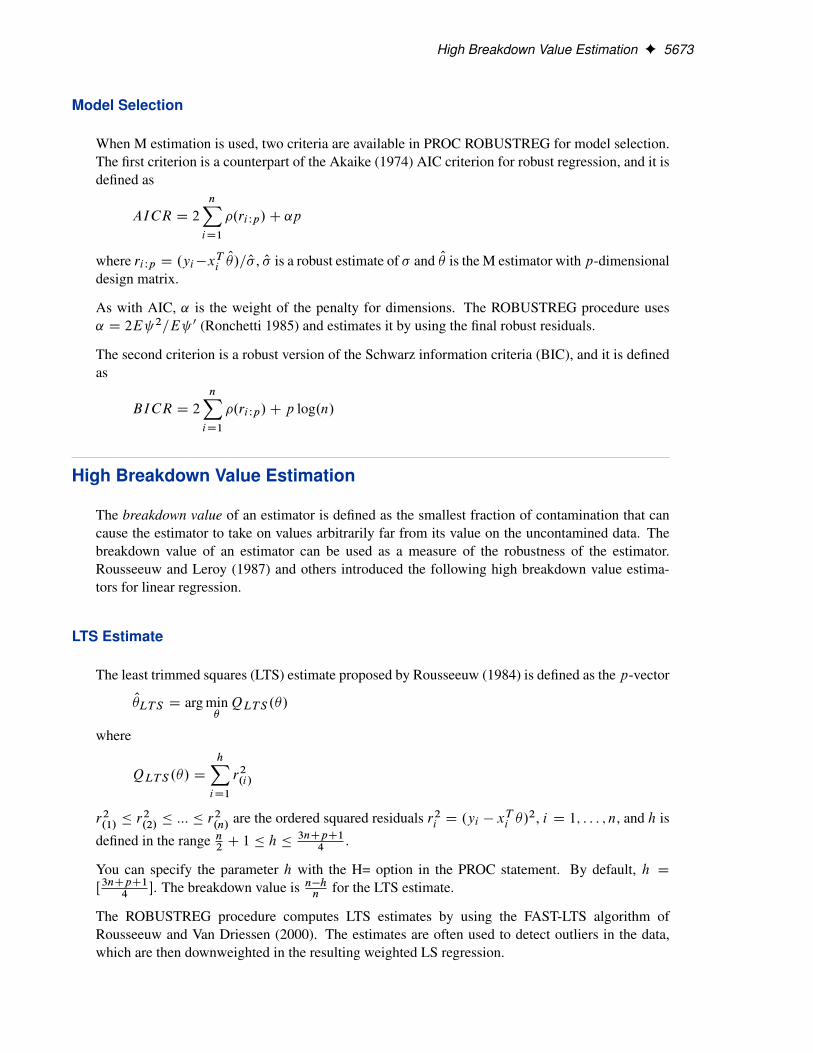
Model Selection
When M estimation is used, two criteria are available in PROC ROBUSTREG for model selection.The first criterion is a counterpart of the Akaike (1974) AIC criterion for robust regression, and it isdefined as
AICR D 2
nXiD1
�.ri Wp/C ˛p
where ri Wp D .yi�xTi
O�/= O� , O� is a robust estimate of � and O� is the M estimator with p-dimensionaldesign matrix.
As with AIC, ˛ is the weight of the penalty for dimensions. The ROBUSTREG procedure uses˛ D 2E 2=E 0 (Ronchetti 1985) and estimates it by using the final robust residuals.
The second criterion is a robust version of the Schwarz information criteria (BIC), and it is definedas
BICR D 2
nXiD1
�.ri Wp/C p log.n/
High Breakdown Value Estimation
The breakdown value of an estimator is defined as the smallest fraction of contamination that cancause the estimator to take on values arbitrarily far from its value on the uncontamined data. Thebreakdown value of an estimator can be used as a measure of the robustness of the estimator.Rousseeuw and Leroy (1987) and others introduced the following high breakdown value estima-tors for linear regression.
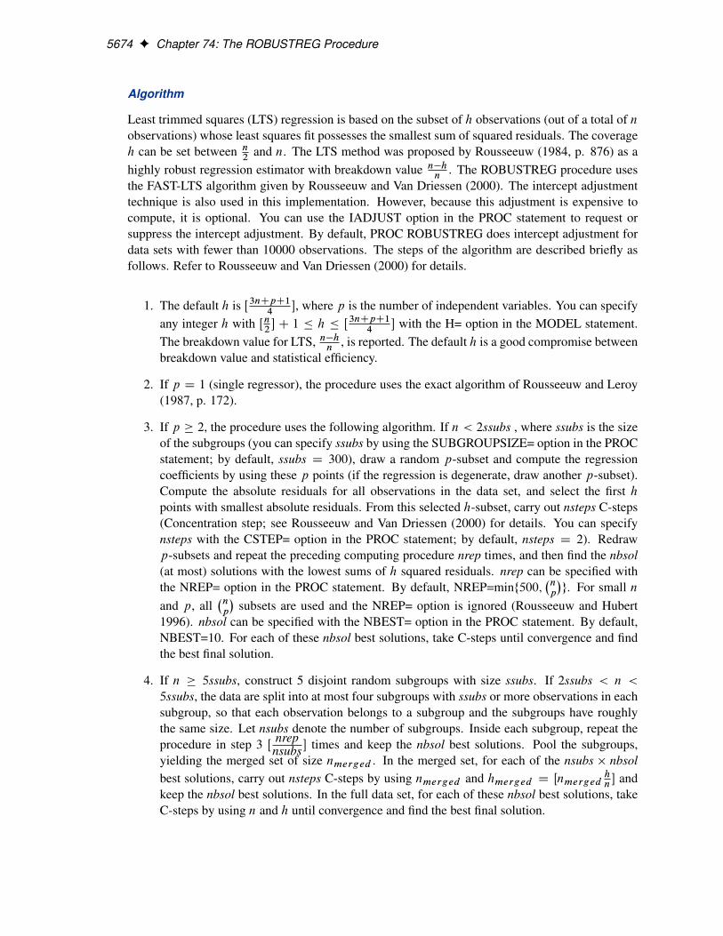
LTS Estimate
The least trimmed squares (LTS) estimate proposed by Rousseeuw (1984) is defined as the p-vector
O�LTS D arg min�QLTS .�/
where
QLTS .�/ D
hXiD1
r2.i/
r2.1/
� r2.2/
� ::: � r2.n/
are the ordered squared residuals r2i D .yi � xTi �/2, i D 1; : : : ; n, and h is
defined in the range n2
C 1 � h �3nCpC1
4.
You can specify the parameter h with the H= option in the PROC statement. By default, h D
Œ3nCpC14
�. The breakdown value is n�hn
for the LTS estimate.
The ROBUSTREG procedure computes LTS estimates by using the FAST-LTS algorithm ofRousseeuw and Van Driessen (2000). The estimates are often used to detect outliers in the data,which are then downweighted in the resulting weighted LS regression.
5674 F Chapter 74: The ROBUSTREG Procedure
Algorithm
Least trimmed squares (LTS) regression is based on the subset of h observations (out of a total of nobservations) whose least squares fit possesses the smallest sum of squared residuals. The coverageh can be set between n
2and n. The LTS method was proposed by Rousseeuw (1984, p. 876) as a
highly robust regression estimator with breakdown value n�hn
. The ROBUSTREG procedure usesthe FAST-LTS algorithm given by Rousseeuw and Van Driessen (2000). The intercept adjustmenttechnique is also used in this implementation. However, because this adjustment is expensive tocompute, it is optional. You can use the IADJUST option in the PROC statement to request orsuppress the intercept adjustment. By default, PROC ROBUSTREG does intercept adjustment fordata sets with fewer than 10000 observations. The steps of the algorithm are described briefly asfollows. Refer to Rousseeuw and Van Driessen (2000) for details.
1. The default h is Œ3nCpC14
�, where p is the number of independent variables. You can specifyany integer h with Œn
2� C 1 � h � Œ3nCpC1
4� with the H= option in the MODEL statement.
The breakdown value for LTS, n�hn
, is reported. The default h is a good compromise betweenbreakdown value and statistical efficiency.
2. If p D 1 (single regressor), the procedure uses the exact algorithm of Rousseeuw and Leroy(1987, p. 172).
3. If p � 2, the procedure uses the following algorithm. If n < 2ssubs , where ssubs is the sizeof the subgroups (you can specify ssubs by using the SUBGROUPSIZE= option in the PROCstatement; by default, ssubs D 300), draw a random p-subset and compute the regressioncoefficients by using these p points (if the regression is degenerate, draw another p-subset).Compute the absolute residuals for all observations in the data set, and select the first hpoints with smallest absolute residuals. From this selected h-subset, carry out nsteps C-steps(Concentration step; see Rousseeuw and Van Driessen (2000) for details. You can specifynsteps with the CSTEP= option in the PROC statement; by default, nsteps D 2). Redrawp-subsets and repeat the preceding computing procedure nrep times, and then find the nbsol(at most) solutions with the lowest sums of h squared residuals. nrep can be specified withthe NREP= option in the PROC statement. By default, NREP=minf500;
�np
�g. For small n
and p, all�np
�subsets are used and the NREP= option is ignored (Rousseeuw and Hubert
1996). nbsol can be specified with the NBEST= option in the PROC statement. By default,NBEST=10. For each of these nbsol best solutions, take C-steps until convergence and findthe best final solution.
4. If n � 5ssubs, construct 5 disjoint random subgroups with size ssubs. If 2ssubs < n <
5ssubs, the data are split into at most four subgroups with ssubs or more observations in eachsubgroup, so that each observation belongs to a subgroup and the subgroups have roughlythe same size. Let nsubs denote the number of subgroups. Inside each subgroup, repeat theprocedure in step 3 Πnrep
nsubs � times and keep the nbsol best solutions. Pool the subgroups,yielding the merged set of size nmerged . In the merged set, for each of the nsubs � nbsolbest solutions, carry out nsteps C-steps by using nmerged and hmerged D Œnmerged
hn� and
keep the nbsol best solutions. In the full data set, for each of these nbsol best solutions, takeC-steps by using n and h until convergence and find the best final solution.

High Breakdown Value Estimation F 5675
R2
The robust version of R2 for the LTS estimate is defined as
R2LTS D 1 �s2LTS .X; y/
s2LTS .1; y/
for models with the intercept term and as
R2LTS D 1 �s2LTS .X; y/
s2LTS .0; y/
for models without the intercept term, where
sLTS .X; y/ D dh;n
vuut1
h
hXiD1
r2.i/
sLTS is a preliminary estimate of the parameter � in the distribution function L.�=�/.
Here dh;n is chosen to make sLTS consistent, assuming a Gaussian model. Specifically,
dh;n D 1=
s1 �
2n
hch;n�.1=ch;n/
ch;n D 1=ˆ�1.hC n
2n/
with ˆ and � being the distribution function and the density function of the standard normal distri-bution, respectively.
Final Weighted Scale Estimator
The ROBUSTREG procedure displays two scale estimators, sLTS and Wscale. The estimator Ws-cale is a more efficient scale estimator based on the preliminary estimate sLTS , and it is definedas
Wscale D
s Pi wir
2iP
i wi � p
where
wi D
�0 if jri j=sLTS > k
1 otherwise
You can specify k with the CUTOFF= option in the MODEL statement. By default, k D 3.
5676 F Chapter 74: The ROBUSTREG Procedure
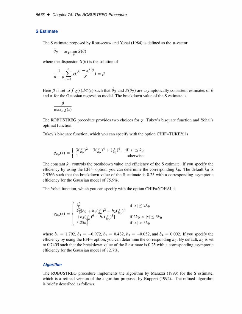
S Estimate
The S estimate proposed by Rousseeuw and Yohai (1984) is defined as the p-vector
O�S D arg min�S.�/
where the dispersion S.�/ is the solution of
1
n � p
nXiD1
�.yi � xTi �
S/ D ˇ
Here ˇ is set toR�.s/dˆ.s/ such that O�S and S. O�S / are asymptotically consistent estimates of �
and � for the Gaussian regression model. The breakdown value of the S estimate is
ˇ
maxs �.s/
The ROBUSTREG procedure provides two choices for �: Tukey’s bisquare function and Yohai’soptimal function.
Tukey’s bisquare function, which you can specify with the option CHIF=TUKEY, is
�k0.s/ D
�3. sk0/2 � 3. s
k0/4 C . s
k0/6; if jsj � k0
1 otherwise
The constant k0 controls the breakdown value and efficiency of the S estimate. If you specify theefficiency by using the EFF= option, you can determine the corresponding k0. The default k0 is2.9366 such that the breakdown value of the S estimate is 0.25 with a corresponding asymptoticefficiency for the Gaussian model of 75:9%.
The Yohai function, which you can specify with the option CHIF=YOHAI, is
�k0.s/ D
8̂̂̂<̂ˆ̂:
s2
2if jsj � 2k0
k20 Œb0 C b1.sk0/2 C b2.
sk0/4
Cb3.sk0/6 C b4.
sk0/8� if 2k0 < jsj � 3k0
3:25k20 if jsj > 3k0
where b0 D 1:792, b1 D �0:972, b2 D 0:432, b3 D �0:052, and b4 D 0:002. If you specify theefficiency by using the EFF= option, you can determine the corresponding k0. By default, k0 is setto 0.7405 such that the breakdown value of the S estimate is 0.25 with a corresponding asymptoticefficiency for the Gaussian model of 72:7%.
Algorithm
The ROBUSTREG procedure implements the algorithm by Marazzi (1993) for the S estimate,which is a refined version of the algorithm proposed by Ruppert (1992). The refined algorithmis briefly described as follows.
High Breakdown Value Estimation F 5677
Initialize iter D 1.
1. Draw a random q-subset of the total n observations and compute the regression coefficientsby using these q observations (if the regression is degenerate, draw another q-subset), whereq � p can be specified with the SUBSIZE= option. By default, q D p.
2. Compute the residuals: ri D yi �PpjD1 xij �j for i D 1; : : : ; n. If iter D 1, set s� D
2medianfjri j; i D 1; : : : ; ng; if s� D 0, set s� D minfjri j; i D 1; : : : ; ng;while
PniD1 �.ri=s
�/ > .n � p/ˇ, set s� D 1:5s�; go to step 3.If iter > 1 and
PniD1 �.ri=s
�/ <D .n � p/ˇ, go to step 3; otherwise, go to step 5.
3. Solve for s the equation
1
n � p
nXiD1
�.ri=s/ D ˇ
using an iterative algorithm.
4. If iter > 1 and s > s�, go to step 5. Otherwise, set s� D s and �� D � . If s� < TOLS ,return s� and ��; otherwise, go to step 5.
5. If iter < NREP , set iter D iter C 1 and return to step 1; otherwise, return s� and ��.
The ROBUSTREG procedure does the following refinement step by default. You can request thatthis refinement not be done by using the NOREFINE option in the PROC statement.
6. Let D �0. Using the values s� and �� from the previous steps, compute M estimates�M and �M of � and � with the setup for M estimation in the section “M Estimation” onpage 5666. If �M > s�, give a warning and return s� and ��; otherwise, return �M and �M .
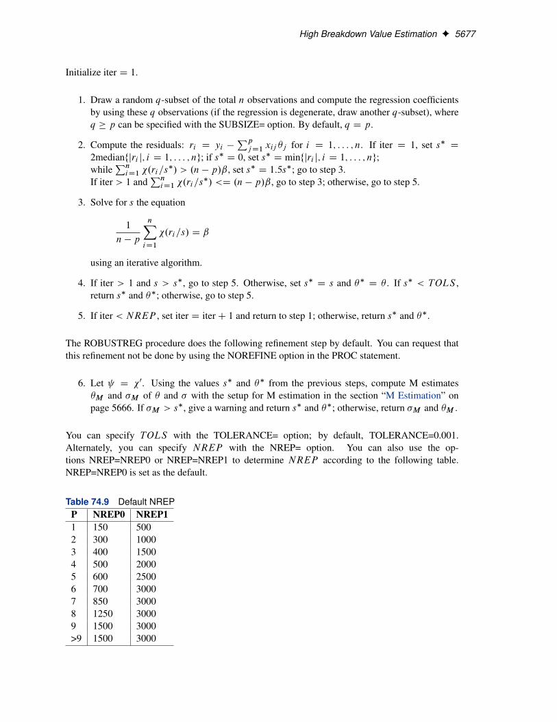
You can specify TOLS with the TOLERANCE= option; by default, TOLERANCE=0.001.Alternately, you can specify NREP with the NREP= option. You can also use the op-tions NREP=NREP0 or NREP=NREP1 to determine NREP according to the following table.NREP=NREP0 is set as the default.
Table 74.9 Default NREPP NREP0 NREP11 150 5002 300 10003 400 15004 500 20005 600 25006 700 30007 850 30008 1250 30009 1500 3000>9 1500 3000
5678 F Chapter 74: The ROBUSTREG Procedure
R2 and Deviance
The robust version of R2 for the S estimate is defined as
R2S D 1 �.n � p/S2p
.n � 1/S2�
for the model with the intercept term and
R2S D 1 �.n � p/S2p
nS20
for the model without the intercept term, where Sp is the S estimate of the scale in the full model,S� is the S estimate of the scale in the regression model with only the intercept term, and S0 is theS estimate of the scale without any regressor. The deviance D is defined as the optimal value of theobjective function on the �2 scale:
D D S2p
Asymptotic Covariance and Confidence Intervals
Since the S estimate satisfies the first-order necessary conditions as the M estimate, it has the sameasymptotic covariance as that of the M estimate. All three estimators of the asymptotic covariancefor the M estimate in the section “Asymptotic Covariance and Confidence Intervals” on page 5671can be used for the S estimate. Besides, the weighted covariance estimator H4 described in thesection “Asymptotic Covariance and Confidence Intervals” on page 5681 is also available and isset as the default. Confidence intervals for estimated parameters are computed from the diagonalelements of the estimated asymptotic covariance matrix.
MM Estimation
MM estimation is a combination of high breakdown value estimation and efficient estimation, whichwas introduced by Yohai (1987). It has the following three steps.
1. Compute an initial (consistent) high breakdown value estimate O� 0. The ROBUSTREG pro-cedure provides two kinds of estimates as the initial estimate: the LTS estimate and the Sestimate. By default, the LTS estimate is used because of its speed and high breakdownvalue. The breakdown value of the final MM estimate is decided by the breakdown valueof the initial LTS estimate and the constant k0 in the � function. To use the S estimate asthe initial estimate, you specify the INITEST=S option in the PROC statement. In this case,the breakdown value of the final MM estimate is decided only by the constant k0. Insteadof computing the LTS estimate or the S estimate as the initial estimate, you can also specifythe initial estimate explicitly by using the INEST= option in the PROC statement. See thesection “INEST= Data Set” on page 5683 for details.
MM Estimation F 5679
2. Find O� 0 such that
1
n � p
nXiD1
�.yi � xTi
O� 0
O� 0/ D ˇ
where ˇ DR�.s/dˆ.s/.
The ROBUSTREG procedure provides two choices for �: Tukey’s bisquare function andYohai’s optimal function.
Tukey’s bisquare function, which you can specify with the option CHIF=TUKEY, is
�k0.s/ D
�3. sk0/2 � 3. s
k0/4 C . s
k0/6; if jsj � k0
1 otherwise
where k0 can be specified with the K0= option. The default k0 is 2.9366 such that the asymp-totically consistent scale estimate O� 0 has the breakdown value of 25%.
Yohai’s optimal function, which you can specify with the option CHIF=YOHAI, is
�k0.s/ D
8̂̂̂<̂ˆ̂:
s2
2if jsj � 2k0
k20 Œb0 C b1.sk0/2 C b2.
sk0/4
Cb3.sk0/6 C b4.
sk0/8� if 2k0 < jsj � 3k0
3:25k20 if jsj > 3k0
where b0 D 1:792, b1 D �0:972, b2 D 0:432, b3 D �0:052, and b4 D 0:002. Youcan specify k0 with the K0= option. The default k0 is 0.7405 such that the asymptoticallyconsistent scale estimate O� 0 has the breakdown value of 25%.
3. Find a local minimum O�MM of
QMM D
nXiD1
�.yi � xTi �
O� 0/
such that QMM . O�MM / � QMM . O� 0/. The algorithm for M estimation is used here.
The ROBUSTREG procedure provides two choices for �: Tukey’s bisquare function andYohai’s optimal function.
Tukey’s bisquare function, which you can specify with the option CHIF=TUKEY, is
�.s/ D �k1.s/ D
�3. sk1/2 � 3. s
k1/4 C . s
k1/6; if jsj � k1
1 otherwise
where k1 can be specified with the K1= option. The default k1 is 3.440 such that the MMestimate has 85% asymptotic efficiency with the Gaussian distribution.
Yohai’s optimal function, which you can specify with the option CHIF=YOHAI, is
�.s/ D �k1.s/ D
8̂̂̂<̂ˆ̂:
s2
2if jsj � 2k1
k21 Œb0 C b1.sk1/2 C b2.
sk1/4
Cb3.sk1/6 C b4.
sk1/8� if 2k1 < jsj � 3k1
3:25k21 if jsj > 3k1
where k1 can be specified with the K1= option. The default k1 is 0.868 such that the MMestimate has 85% asymptotic efficiency with the Gaussian distribution.
5680 F Chapter 74: The ROBUSTREG Procedure
Algorithm
The initial LTS estimate is computed using the algorithm described in the section “LTS Estimate”on page 5673. You can control the quantile of the LTS estimate with the option INITH=h, where his an integer between Œn
2� C 1 and Œ3nCpC1
4�. By default, h D Œ3nCpC1
4�, which corresponds to a
breakdown value of around 25%.
The initial S estimate is computed using the algorithm described in the section “S Estimate” onpage 5676. You can control the breakdown value and efficiency of this initial S estimate by theconstant k0, which can be specified with the K0 option.
The scale parameter � is solved by an iterative algorithm
.� .mC1//2 D1
.n � p/ˇ
nXiD1
�k0.ri
� .m//.� .m//2
where ˇ DR�k0
.s/dˆ.s/.
Once the scale parameter is computed, the iteratively reweighted least squares (IRLS) algorithmwith fixed scale parameter is used to compute the final MM estimate.
Convergence Criteria
In the iterative algorithm for the scale parameter, the relative change of the scale parameter controlsthe convergence.
In the iteratively reweighted least squares algorithm, the same convergence criteria for the M esti-mate used before are used here.
Bias Test
Although the final MM estimate inherits the high breakdown value property, its bias due to thedistortion of the outliers can be high. Yohai, Stahel, and Zamar (1991) introduced a bias test. TheROBUSTREG procedure implements this test when you specify the BIASTEST option in the PROCstatement. This test is based on the initial scale estimate O� 0 and the final scale estimate O� 0
1, which isthe solution of
1
n � p
nXiD1
�.yi � xTi
O�MM
O� 01
/ D ˇ
Let k0.z/ D
@�k0.z/
@zand k1
.z/ D@�k1
.z/
@z. Compute
Qri D .yi � xTiO� 0/= O� 0 for i D 1; : : : ; n
v0 D.1=n/
P 0k0. Qri /
. O� 01=n/
P k0
. Qri / Qri
MM Estimation F 5681
p.0/i D
k0. Qri /
.1=n/P 0k0. Qri /
for i D 1; : : : ; n
p.1/i D
k1. Qri /
.1=n/P 0k1. Qri /
for i D 1; : : : ; n
d2 D1
n
X.p.1/i � p
.0/i /2
Let
T D2n. O� 0
1 � O� 0/
v0d2. O� 0/2
Standard asymptotic theory shows that T approximately follows a �2 distribution with p degreesof freedom. If T exceeds the ˛ quantile �2˛ of the �2 distribution with p degrees of freedom,then the ROBUSTREG procedure gives a warning and recommends that you use other methods.Otherwise the final MM estimate and the initial scale estimate are reported. You can specify ˛ withthe ALPHA= option following the BIASTEST option. By default, ALPHA=0.99.
Asymptotic Covariance and Confidence Intervals
Since the MM estimate is computed as a M estimate with a fixed scale in the last step, the asymptoticcovariance for the M estimate can be used here for the asymptotic covariance of the MM estimate.Besides the three estimators H1, H2, and H3 as described in the section “Asymptotic Covarianceand Confidence Intervals” on page 5671, a weighted covariance estimator H4 is available:
H4: K2Œ1=.n � p/�
P. .ri //
2
Œ.1=n/P. 0.ri //�2
W �1
where K D 1Cpn
Var. 0/
.E 0/2is the correction factor and Wjk D
1Nw
Pwixijxik , Nw D
1n
Pwi .
You can specify these estimators with the option ASYMPCOV= [H1 | H2 | H3 | H4]. The RO-BUSTREG procedure uses H4 as the default. Confidence intervals for estimated parameters arecomputed from the diagonal elements of the estimated asymptotic covariance matrix.
R Square and Deviance
The robust version of R2 for the MM estimate is defined as
R2 D
P�.yi � O�
Os/ �
P�.yi �xT
iO�
Os/P
�.yi � O�Os/
and the robust deviance is defined as the optimal value of the objective function on the �2 scale:
D D 2.Os/2X
�.yi � xTi
O�
Os/
where �0 D , O� is the MM estimator of � , O� is the MM estimator of location, and Os is the MMestimator of the scale parameter in the full model.
5682 F Chapter 74: The ROBUSTREG Procedure
Linear Tests
For MM estimation, the same � test and R2n test used for M estimation can be used. See the section“Linear Tests” on page 5672 for details.
Model Selection
For MM estimation, the same two model selection methods used for M estimation can be used. Seethe section “Model Selection” on page 5673 for details.
Robust Distance
The ROBUSTREG procedure uses the robust multivariate location and scale estimates for leverage-point detection. The procedure computes a robust version of the Mahalanobis distance by using theminimum covariance determinant (MCD) method of Rousseeuw (1984).
Algorithm
PROC ROBUSTREG implements the algorithm given by Rousseeuw and Van Driessen (1999) forMCD, which is similar to the algorithm for LTS.
Robust Distance
The Mahalanobis distance is defined as
MD.xi / D Œ.xi � Nx/T NC.X/�1.xi � Nx/�1=2
where Nx D1n
PniD1 xi and NC.X/ D
1n�1
PniD1.xi � Nx/T .xi � Nx/ are the empirical multivariate
location and scale. Here xi D .xi1; : : : ; xi.p�1//T does not include the intercept. The relation
between the Mahalanobis distance MD.xi / and the hat matrix H D .hij / D X.XTX/�1XT is
hi i D1
n � 1MD2i C
1
n
The robust distance is defined as
RD.xi / D Œ.xi � T .X//TC.X/�1.xi � T .X//�1=2
where T .X/ and C.X/ are the robust multivariate location and scale obtained by MCD.
These distances are used to detect leverage points.
Leverage Point and Outlier Detection F 5683
Leverage Point and Outlier Detection
Let C.p/ D
q�2pI1�˛ be the cutoff value. The variable LEVERAGE is defined as
LEVERAGE D
�0 if RD.xi / � C.p/
1 otherwise
You can specify a cutoff value with the LEVERAGE option in the MODEL statement.
Residuals ri ; i D 1; : : : ; n, based on robust regression estimates are used to detect vertical outliers.The variable OUTLIER is defined as
OUTLIER D
�0 if jri j � k O�
1 otherwise
You can specify the multiplier k of the cutoff value by using the CUTOFF= option in the MODELstatement. By default, k D 3. O� is estimated scale in the model.
An ODS table called DIAGNOSTICS contains these two variables.
INEST= Data Set
When you use the M or MM estimation, you can use the INEST= data set to specify initial estimatesfor all the parameters in the model. The INEST= option is ignored if you specify LTS or S estimationby using the METHOD=LTS or METHOD=S option or if you specify the INITEST= option afterthe METHOD=MM option in the PROC statement. The INEST= data set must contain the interceptvariable (named Intercept) and all independent variables in the MODEL statement.
If BY processing is used, the INEST= data set should also include the BY variables, and there mustbe at least one observation for each BY group. If there is more than one observation in a BY group,the first one read is used for that BY group.
If the INEST= data set also contains the _TYPE_ variable, only observations with _TYPE_ value“PARMS” are used as starting values.
You can specify starting values for the iteratively reweighted least squares algorithm in the INEST=data set. The INEST= data set has the same structure as the OUTEST= data set but is not requiredto have all the variables or observations that appear in the OUTEST= data set. One simple use of theINEST= option is passing the previous OUTEST= data set directly to the next model as an INEST=data set, assuming that the two models have the same parameterization.
5684 F Chapter 74: The ROBUSTREG Procedure
OUTEST= Data Set
The OUTEST= data set contains parameter estimates for the model. You can specify a label in theMODEL statement to distinguish between the estimates for different models used by the ROBUS-TREG procedure. If the COVOUT option is specified, the OUTEST= data set also contains theestimated covariance matrix of the parameter estimates. Note that, if the ROBUSTREG proceduredoes not converge, the parameter estimates are set to missing in the OUTEST data set.
The OUTEST= data set contains all variables specified in the MODEL statement and the BY state-ment. One observation consists of parameter values for the model with the dependent variablehaving the value �1. If the COVOUT option is specified, there are additional observations con-taining the rows of the estimated covariance matrix. For these observations, the dependent variablecontains the parameter estimate for the corresponding row variable. The following variables arealso added to the data set:
_MODEL_ is a character variable containing the label of the MODEL statement, if present.Otherwise, the variable’s value is blank.
_NAME_ is a character variable containing the name of the dependent variable for theparameter estimates or the name of the row for the covariance matrix estimates.
_TYPE_ is a character variable containing the type of the observation, either PARMS forparameter estimates or COV for covariance estimates.
_METHOD_ is a character variable containing the type of estimation method, either M esti-mation, LTS estimation, S estimation, or MM estimation.
_STATUS_ is a character variable containing the status of model fitting, either Converged,Warning, or Failed.
INTERCEPT is a numeric variable containing the intercept parameter estimates and covari-ances.
_SCALE_ is a numeric variable containing the scale parameter estimates.
Any BY variables specified are also added to the OUTEST= data set.
Computational Resources
The algorithms for the various estimation methods need a different amount of memory for workingspace. Let p be the number of parameters estimated and n be the number of observations used inthe model estimation.
For M estimation, the minimum working space (in bytes) needed is
3nC 2p2 C 30p
If sufficient space is available, the input data set is also kept in memory; otherwise, the input dataset is reread for computing the iteratively reweighted least squares estimates and the execution
ODS Table Names F 5685
time of the procedure increases substantially. For each reweighted least squares, O.np2 C p3/
multiplications and additions are required for computing the crossproduct matrix and its inverse.TheO.v/ notation means that, for large values of the argument, v,O.v/ is approximately a constanttimes v.
Since the iteratively reweighted least squares algorithm converges very quickly (normally withinfewer than 20 iterations), the computation of M estimates is fast.
LTS estimation is more expensive in computation. The minimum working space (in bytes) neededis
np C 12nC 4p2 C 60p
The memory is mainly used to store the current data used by LTS for modeling. The LTS algorithmuses subsampling and spends much of its computing time on resampling and computing estimatesfor subsamples. Since it resamples if singularity is detected, it might take more time if the data sethas serious singularities.
The MCD algorithm for leverage-point diagnostics is similar to the LTS algorithm.
ODS Table Names
The ROBUSTREG procedure assigns a name to each table it creates. You can specify these nameswhen using the Output Delivery System (ODS) to select tables and create output data sets. Thesenames are listed in the following table.
Table 74.10 ODS Tables Produced by PROC ROBUSTREG
ODS Table Name Description Statement OptionBestEstimates Best final estimates for LTS PROC SUBANALYSISBestSubEstimates Best estimates for each subgroup PROC SUBANALYSISBiasTest Bias test for MM estimation PROC BIASTESTClassLevels Classification variable levels CLASS defaultCorrB Parameter estimate correlation matrix MODEL CORRBCovB Parameter estimate covariance matrix MODEL COVBCStep C-step for LTS fitting PROC SUBANALYSISDiagnostics Outlier diagnostics MODEL DIAGNOSTICSDiagSummary Summary of the outlier diagnostics MODEL defaultGoodFit R2, deviance, AIC, and BIC MODEL METHODInitLTSProfile Profile for initial LTS estimate PROC METHODInitSProfile Profile for initial S estimate PROC METHODIterHistory Iteration history PROC ITPRINTLTSEstimates LTS parameter estimates PROC METHODLTSLocationScale Location and scale for LTS PROC METHODLTSProfile Profile for LTS estimator PROC METHODLTSRsquare R2 for LTS estimate PROC METHODMMProfile Profile for MM estimator PROC METHODModelInfo Model information MODEL default
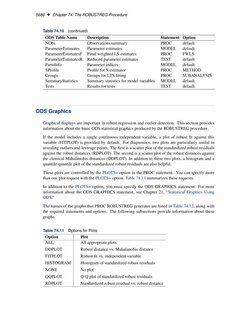
5686 F Chapter 74: The ROBUSTREG Procedure
Table 74.10 (continued)
ODS Table Name Description Statement OptionNObs Observations summary PROC defaultParameterEstimates Parameter estimates MODEL defaultParameterEstimatesF Final weighted LS estimates PROC FWLSParameterEstimatesR Reduced parameter estimates TEST defaultParmInfo Parameter indices MODEL defaultSProfile Profile for S estimator PROC METHODGroups Groups for LTS fitting PROC SUBANALYSISSummaryStatistics Summary statistics for model variables MODEL defaultTests Results for tests TEST default
ODS Graphics
Graphical displays are important in robust regression and outlier detection. This section providesinformation about the basic ODS statistical graphics produced by the ROBUSTREG procedure.
If the model includes a single continuous independent variable, a plot of robust fit against thisvariable (FITPLOT) is provided by default. For diagnostics, two plots are particularly useful inrevealing outliers and leverage points. The first is a scatter plot of the standardized robust residualsagainst the robust distances (RDPLOT). The second is a scatter plot of the robust distances againstthe classical Mahalanobis distances (DDPLOT). In addition to these two plots, a histogram and aquantile-quantile plot of the standardized robust residuals are also helpful.
These plots are controlled by the PLOTS= option in the PROC statement. You can specify morethan one plot request with the PLOTS= option. Table 74.11 summarizes these requests.
In addition to the PLOTS= option, you must specify the ODS GRAPHICS statement. For moreinformation about the ODS GRAPHICS statement, see Chapter 21, “Statistical Graphics UsingODS.”
The names of the graphs that PROC ROBUSTREG generates are listed in Table 74.12, along withthe required statements and options. The following subsections provide information about thesegraphs.
Table 74.11 Options for Plots
Option PlotALL All appropriate plots
DDPLOT Robust distance vs. Mahalanobis distance
FITPLOT Robust fit vs. independent variable
HISTOGRAM Histogram of standardized robust residuals
NONE No plot
QQPLOT Q-Q plot of standardized robust residuals
RDPLOT Standardized robust residual vs. robust distance
ODS Graphics F 5687
Fit Plot
When the model has a single independent continuous variable (with or without the intercept), theROBUSTREG procedure automatically creates a plot of robust fit against this independent variable.
The following simple example is used to show the fit plot. The data, from Rousseeuw and Leroy(1987, Table 3), include the logarithm of surface temperature and the logarithm of light intensityfor 47 stars in the direction of the constellation Cygnus.
data star;input index x y @@;label x = ’Log Temperature’
y = ’Log Light Intensity’;datalines;1 4.37 5.23 25 4.38 5.022 4.56 5.74 26 4.42 4.663 4.26 4.93 27 4.29 4.664 4.56 5.74 28 4.38 4.905 4.30 5.19 29 4.22 4.396 4.46 5.46 30 3.48 6.057 3.84 4.65 31 4.38 4.428 4.57 5.27 32 4.56 5.109 4.26 5.57 33 4.45 5.2210 4.37 5.12 34 3.49 6.2911 3.49 5.73 35 4.23 4.3412 4.43 5.45 36 4.62 5.6213 4.48 5.42 37 4.53 5.1014 4.01 4.05 38 4.45 5.2215 4.29 4.26 39 4.53 5.1816 4.42 4.58 40 4.43 5.5717 4.23 3.94 41 4.38 4.6218 4.42 4.18 42 4.45 5.0619 4.23 4.18 43 4.50 5.3420 3.49 5.89 44 4.45 5.3421 4.29 4.38 45 4.55 5.5422 4.29 4.22 46 4.45 4.9823 4.42 4.42 47 4.42 4.5024 4.49 4.85;
The fit plot in Figure 74.17, created with the following statements, plots the robust fit of the loga-rithm of light intensity with the MM method against the logarithm of the surface temperature.
ods graphics on;
proc robustreg data=star method=mm ;model y = x;
run;
ods graphics off;
Confidence limits are added on the plot by default. The NOLIMITS option suppresses these limits.
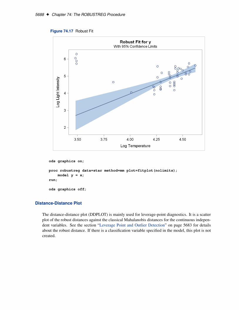
5688 F Chapter 74: The ROBUSTREG Procedure
Figure 74.17 Robust Fit
ods graphics on;
proc robustreg data=star method=mm plot=fitplot(nolimits);model y = x;
run;
ods graphics off;
Distance-Distance Plot
The distance-distance plot (DDPLOT) is mainly used for leverage-point diagnostics. It is a scatterplot of the robust distances against the classical Mahalanobis distances for the continuous indepen-dent variables. See the section “Leverage Point and Outlier Detection” on page 5683 for detailsabout the robust distance. If there is a classification variable specified in the model, this plot is notcreated.
ODS Graphics F 5689
You can use the PLOT=DDPLOT option to request this plot. The following statements use the stackdata set in the section “M Estimation” on page 5643 to create the single plot shown in Figure 74.5.
ods graphics on;
proc robustreg data=stack plot=ddplot;model y = x1 x2 x3;
run;
ods graphics off;
The reference lines represent the cutoff values. The diagonal line is also drawn to show the dis-tribution of the distances. By default, all outliers and leverage points are labeled with observationnumbers. To change the default, you can use the LABEL= option as described in Table 74.2.
If you specify ID variables in the ID statement, instead of observation numbers, the values of thefirst ID variable are used as labels.
Residual-Distance Plot
The residual-distance plot (RDPLOT) is used for both outlier and leverage-point diagnostics. Itis a scatter plot of the standardized robust residuals against the robust distances. See the section“Leverage Point and Outlier Detection” on page 5683 for details about the robust distance. If thereis a classification variable specified in the model, this plot is not created.
You can use the PLOT=RDPLOT option to request this plot. The following statements use the stackdata set in the section “M Estimation” on page 5643 to create a single plot shown in Figure 74.4.
ods graphics on;
proc robustreg data=stack plot=rdplot;model y = x1 x2 x3;
run;
ods graphics off;
The reference lines represent the cutoff values. By default, all outliers and leverage points arelabeled with observation numbers. To change the default, you can use the LABEL= option asdescribed in Table 74.2.
If you specify ID variables in the ID statement instead of observation numbers, the values of thefirst ID variable are used as labels.
Histogram and Q-Q Plot
PROC ROBUSTREG produces a histogram and a Q-Q plot for the standardized robust residuals.The histogram is superimposed with a normal density curve and a kernel density curve. Using thestack data set in the section “M Estimation” on page 5643, the following statements create the plotsin Figure 74.6 and Figure 74.7.
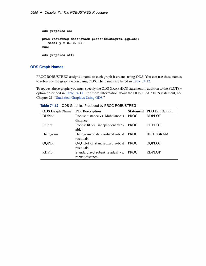
5690 F Chapter 74: The ROBUSTREG Procedure
ods graphics on;
proc robustreg data=stack plots=(histogram qqplot);model y = x1 x2 x3;
run;
ods graphics off;
ODS Graph Names
PROC ROBUSTREG assigns a name to each graph it creates using ODS. You can use these namesto reference the graphs when using ODS. The names are listed in Table 74.12.
To request these graphs you must specify the ODS GRAPHICS statement in addition to the PLOTS=option described in Table 74.11. For more information about the ODS GRAPHICS statement, seeChapter 21, “Statistical Graphics Using ODS.”
Table 74.12 ODS Graphics Produced by PROC ROBUSTREG
ODS Graph Name Plot Description Statement PLOTS= OptionDDPlot Robust distance vs. Mahalanobis
distancePROC DDPLOT
FitPlot Robust fit vs. independent vari-able
PROC FITPLOT
Histogram Histogram of standardized robustresiduals
PROC HISTOGRAM
QQPlot Q-Q plot of standardized robustresiduals
PROC QQPLOT
RDPlot Standardized robust residual vs.robust distance
PROC RDPLOT
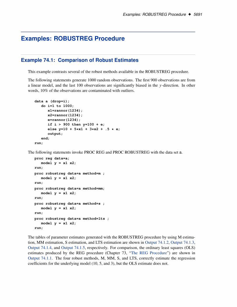
Examples: ROBUSTREG Procedure F 5691
Examples: ROBUSTREG Procedure
Example 74.1: Comparison of Robust Estimates
This example contrasts several of the robust methods available in the ROBUSTREG procedure.
The following statements generate 1000 random observations. The first 900 observations are froma linear model, and the last 100 observations are significantly biased in the y-direction. In otherwords, 10% of the observations are contaminated with outliers.
data a (drop=i);do i=1 to 1000;
x1=rannor(1234);x2=rannor(1234);e=rannor(1234);if i > 900 then y=100 + e;else y=10 + 5*x1 + 3*x2 + .5 * e;output;
end;run;
The following statements invoke PROC REG and PROC ROBUSTREG with the data set a.proc reg data=a;
model y = x1 x2;run;
proc robustreg data=a method=m ;model y = x1 x2;
run;
proc robustreg data=a method=mm;model y = x1 x2;
run;
proc robustreg data=a method=s ;model y = x1 x2;
run;
proc robustreg data=a method=lts ;model y = x1 x2;
run;
The tables of parameter estimates generated with the ROBUSTREG procedure by using M estima-tion, MM estimation, S estimation, and LTS estimation are shown in Output 74.1.2, Output 74.1.3,Output 74.1.4, and Output 74.1.5, respectively. For comparison, the ordinary least squares (OLS)estimates produced by the REG procedure (Chapter 73, “The REG Procedure”) are shown inOutput 74.1.1. The four robust methods, M, MM, S, and LTS, correctly estimate the regressioncoefficients for the underlying model (10, 5, and 3), but the OLS estimate does not.
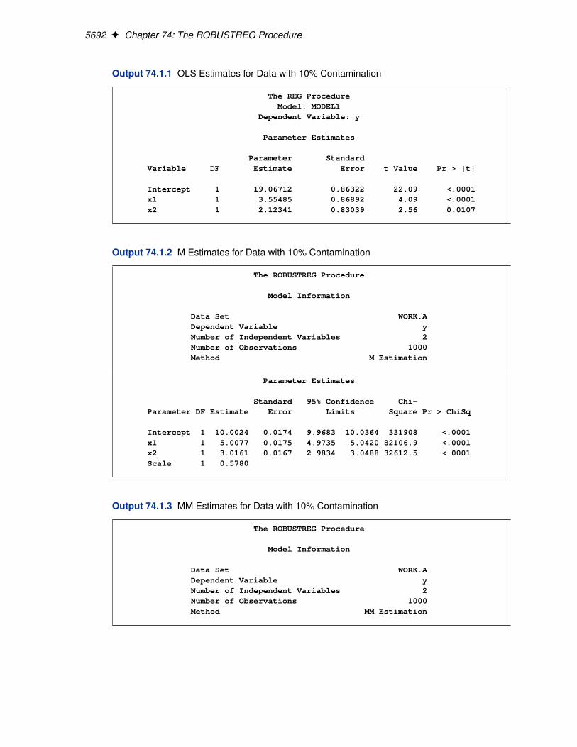
5692 F Chapter 74: The ROBUSTREG Procedure
Output 74.1.1 OLS Estimates for Data with 10% Contamination
The REG ProcedureModel: MODEL1
Dependent Variable: y
Parameter Estimates
Parameter StandardVariable DF Estimate Error t Value Pr > |t|
Intercept 1 19.06712 0.86322 22.09 <.0001x1 1 3.55485 0.86892 4.09 <.0001x2 1 2.12341 0.83039 2.56 0.0107
Output 74.1.2 M Estimates for Data with 10% Contamination
The ROBUSTREG Procedure
Model Information
Data Set WORK.ADependent Variable yNumber of Independent Variables 2Number of Observations 1000Method M Estimation
Parameter Estimates
Standard 95% Confidence Chi-Parameter DF Estimate Error Limits Square Pr > ChiSq
Intercept 1 10.0024 0.0174 9.9683 10.0364 331908 <.0001x1 1 5.0077 0.0175 4.9735 5.0420 82106.9 <.0001x2 1 3.0161 0.0167 2.9834 3.0488 32612.5 <.0001Scale 1 0.5780
Output 74.1.3 MM Estimates for Data with 10% Contamination
The ROBUSTREG Procedure
Model Information
Data Set WORK.ADependent Variable yNumber of Independent Variables 2Number of Observations 1000Method MM Estimation
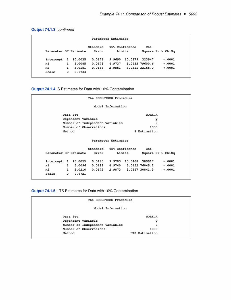
Example 74.1: Comparison of Robust Estimates F 5693
Output 74.1.3 continued
Parameter Estimates
Standard 95% Confidence Chi-Parameter DF Estimate Error Limits Square Pr > ChiSq
Intercept 1 10.0035 0.0176 9.9690 10.0379 323947 <.0001x1 1 5.0085 0.0178 4.9737 5.0433 79600.6 <.0001x2 1 3.0181 0.0168 2.9851 3.0511 32165.0 <.0001Scale 0 0.6733
Output 74.1.4 S Estimates for Data with 10% Contamination
The ROBUSTREG Procedure
Model Information
Data Set WORK.ADependent Variable yNumber of Independent Variables 2Number of Observations 1000Method S Estimation
Parameter Estimates
Standard 95% Confidence Chi-Parameter DF Estimate Error Limits Square Pr > ChiSq
Intercept 1 10.0055 0.0180 9.9703 10.0408 309917 <.0001x1 1 5.0096 0.0182 4.9740 5.0452 76045.2 <.0001x2 1 3.0210 0.0172 2.9873 3.0547 30841.3 <.0001Scale 0 0.6721
Output 74.1.5 LTS Estimates for Data with 10% Contamination
The ROBUSTREG Procedure
Model Information
Data Set WORK.ADependent Variable yNumber of Independent Variables 2Number of Observations 1000Method LTS Estimation
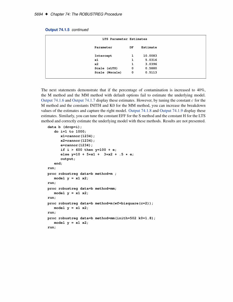
5694 F Chapter 74: The ROBUSTREG Procedure
Output 74.1.5 continued
LTS Parameter Estimates
Parameter DF Estimate
Intercept 1 10.0083x1 1 5.0316x2 1 3.0396Scale (sLTS) 0 0.5880Scale (Wscale) 0 0.5113
The next statements demonstrate that if the percentage of contamination is increased to 40%,the M method and the MM method with default options fail to estimate the underlying model.Output 74.1.6 and Output 74.1.7 display these estimates. However, by tuning the constant c for theM method and the constants INITH and K0 for the MM method, you can increase the breakdownvalues of the estimates and capture the right model. Output 74.1.8 and Output 74.1.9 display theseestimates. Similarly, you can tune the constant EFF for the S method and the constant H for the LTSmethod and correctly estimate the underlying model with these methods. Results are not presented.
data b (drop=i);do i=1 to 1000;
x1=rannor(1234);x2=rannor(1234);e=rannor(1234);if i > 600 then y=100 + e;else y=10 + 5*x1 + 3*x2 + .5 * e;output;
end;run;
proc robustreg data=b method=m ;model y = x1 x2;
run;
proc robustreg data=b method=mm;model y = x1 x2;
run;
proc robustreg data=b method=m(wf=bisquare(c=2));model y = x1 x2;
run;
proc robustreg data=b method=mm(inith=502 k0=1.8);model y = x1 x2;
run;
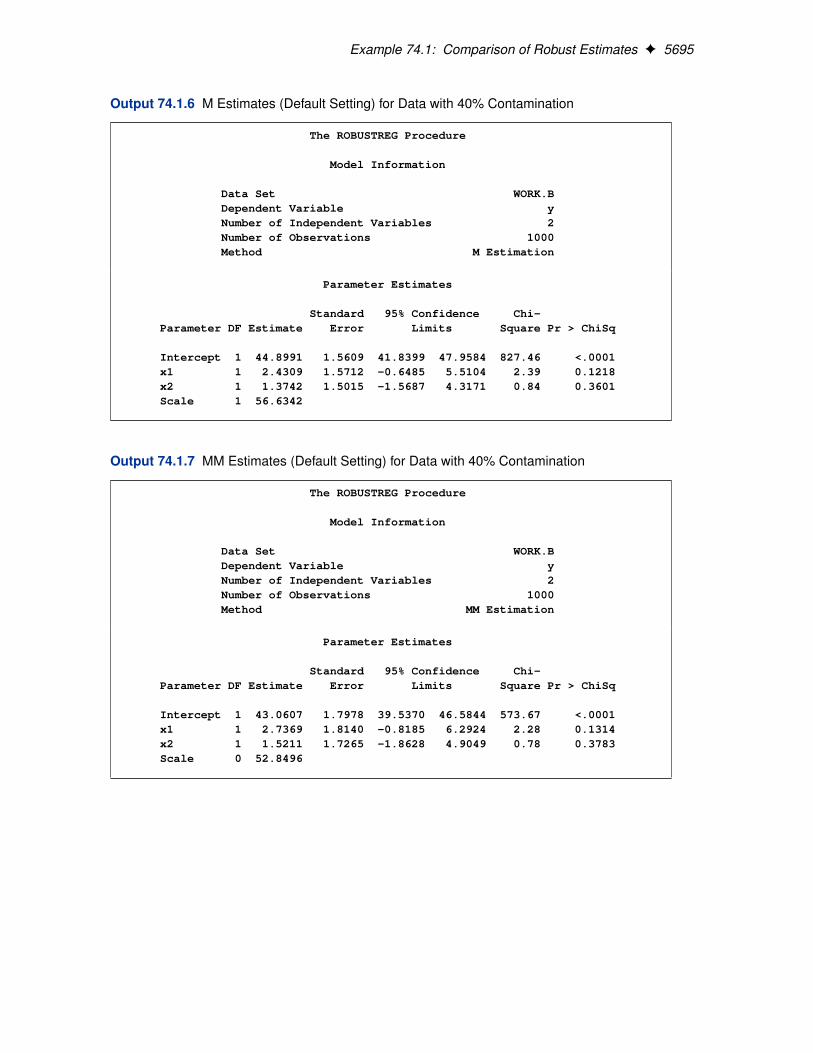
Example 74.1: Comparison of Robust Estimates F 5695
Output 74.1.6 M Estimates (Default Setting) for Data with 40% Contamination
The ROBUSTREG Procedure
Model Information
Data Set WORK.BDependent Variable yNumber of Independent Variables 2Number of Observations 1000Method M Estimation
Parameter Estimates
Standard 95% Confidence Chi-Parameter DF Estimate Error Limits Square Pr > ChiSq
Intercept 1 44.8991 1.5609 41.8399 47.9584 827.46 <.0001x1 1 2.4309 1.5712 -0.6485 5.5104 2.39 0.1218x2 1 1.3742 1.5015 -1.5687 4.3171 0.84 0.3601Scale 1 56.6342
Output 74.1.7 MM Estimates (Default Setting) for Data with 40% Contamination
The ROBUSTREG Procedure
Model Information
Data Set WORK.BDependent Variable yNumber of Independent Variables 2Number of Observations 1000Method MM Estimation
Parameter Estimates
Standard 95% Confidence Chi-Parameter DF Estimate Error Limits Square Pr > ChiSq
Intercept 1 43.0607 1.7978 39.5370 46.5844 573.67 <.0001x1 1 2.7369 1.8140 -0.8185 6.2924 2.28 0.1314x2 1 1.5211 1.7265 -1.8628 4.9049 0.78 0.3783Scale 0 52.8496
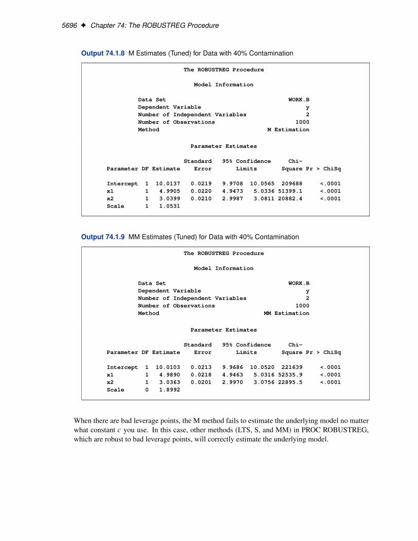
5696 F Chapter 74: The ROBUSTREG Procedure
Output 74.1.8 M Estimates (Tuned) for Data with 40% Contamination
The ROBUSTREG Procedure
Model Information
Data Set WORK.BDependent Variable yNumber of Independent Variables 2Number of Observations 1000Method M Estimation
Parameter Estimates
Standard 95% Confidence Chi-Parameter DF Estimate Error Limits Square Pr > ChiSq
Intercept 1 10.0137 0.0219 9.9708 10.0565 209688 <.0001x1 1 4.9905 0.0220 4.9473 5.0336 51399.1 <.0001x2 1 3.0399 0.0210 2.9987 3.0811 20882.4 <.0001Scale 1 1.0531
Output 74.1.9 MM Estimates (Tuned) for Data with 40% Contamination
The ROBUSTREG Procedure
Model Information
Data Set WORK.BDependent Variable yNumber of Independent Variables 2Number of Observations 1000Method MM Estimation
Parameter Estimates
Standard 95% Confidence Chi-Parameter DF Estimate Error Limits Square Pr > ChiSq
Intercept 1 10.0103 0.0213 9.9686 10.0520 221639 <.0001x1 1 4.9890 0.0218 4.9463 5.0316 52535.9 <.0001x2 1 3.0363 0.0201 2.9970 3.0756 22895.5 <.0001Scale 0 1.8992
When there are bad leverage points, the M method fails to estimate the underlying model no matterwhat constant c you use. In this case, other methods (LTS, S, and MM) in PROC ROBUSTREG,which are robust to bad leverage points, will correctly estimate the underlying model.
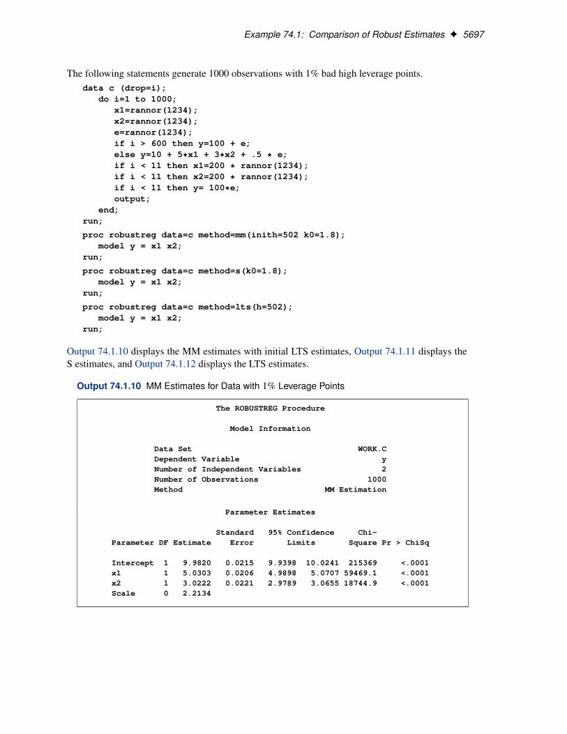
Example 74.1: Comparison of Robust Estimates F 5697
The following statements generate 1000 observations with 1% bad high leverage points.data c (drop=i);
do i=1 to 1000;x1=rannor(1234);x2=rannor(1234);e=rannor(1234);if i > 600 then y=100 + e;else y=10 + 5*x1 + 3*x2 + .5 * e;if i < 11 then x1=200 * rannor(1234);if i < 11 then x2=200 * rannor(1234);if i < 11 then y= 100*e;output;
end;run;
proc robustreg data=c method=mm(inith=502 k0=1.8);model y = x1 x2;
run;
proc robustreg data=c method=s(k0=1.8);model y = x1 x2;
run;
proc robustreg data=c method=lts(h=502);model y = x1 x2;
run;
Output 74.1.10 displays the MM estimates with initial LTS estimates, Output 74.1.11 displays theS estimates, and Output 74.1.12 displays the LTS estimates.
Output 74.1.10 MM Estimates for Data with 1% Leverage Points
The ROBUSTREG Procedure
Model Information
Data Set WORK.CDependent Variable yNumber of Independent Variables 2Number of Observations 1000Method MM Estimation
Parameter Estimates
Standard 95% Confidence Chi-Parameter DF Estimate Error Limits Square Pr > ChiSq
Intercept 1 9.9820 0.0215 9.9398 10.0241 215369 <.0001x1 1 5.0303 0.0206 4.9898 5.0707 59469.1 <.0001x2 1 3.0222 0.0221 2.9789 3.0655 18744.9 <.0001Scale 0 2.2134
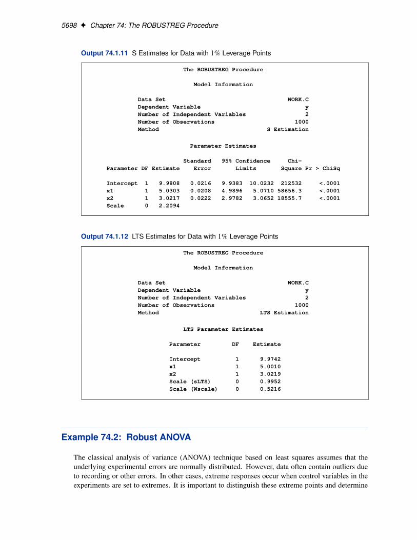
5698 F Chapter 74: The ROBUSTREG Procedure
Output 74.1.11 S Estimates for Data with 1% Leverage Points
The ROBUSTREG Procedure
Model Information
Data Set WORK.CDependent Variable yNumber of Independent Variables 2Number of Observations 1000Method S Estimation
Parameter Estimates
Standard 95% Confidence Chi-Parameter DF Estimate Error Limits Square Pr > ChiSq
Intercept 1 9.9808 0.0216 9.9383 10.0232 212532 <.0001x1 1 5.0303 0.0208 4.9896 5.0710 58656.3 <.0001x2 1 3.0217 0.0222 2.9782 3.0652 18555.7 <.0001Scale 0 2.2094
Output 74.1.12 LTS Estimates for Data with 1% Leverage Points
The ROBUSTREG Procedure
Model Information
Data Set WORK.CDependent Variable yNumber of Independent Variables 2Number of Observations 1000Method LTS Estimation
LTS Parameter Estimates
Parameter DF Estimate
Intercept 1 9.9742x1 1 5.0010x2 1 3.0219Scale (sLTS) 0 0.9952Scale (Wscale) 0 0.5216
Example 74.2: Robust ANOVA
The classical analysis of variance (ANOVA) technique based on least squares assumes that theunderlying experimental errors are normally distributed. However, data often contain outliers dueto recording or other errors. In other cases, extreme responses occur when control variables in theexperiments are set to extremes. It is important to distinguish these extreme points and determine
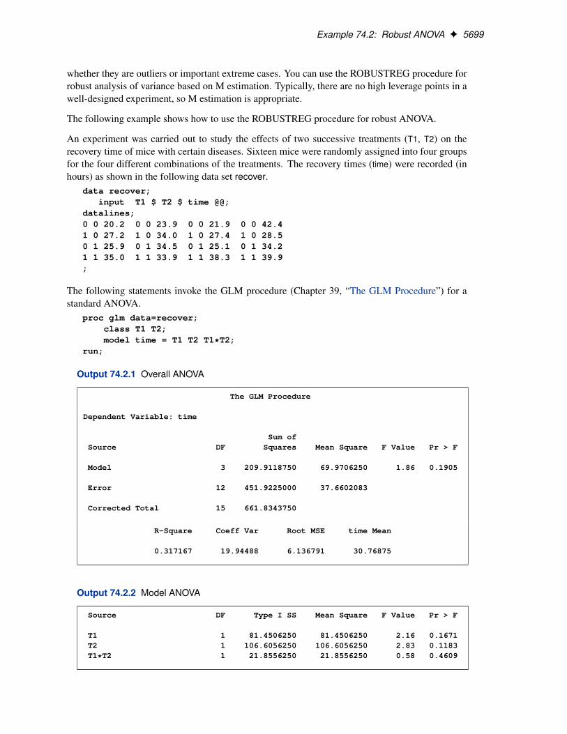
Example 74.2: Robust ANOVA F 5699
whether they are outliers or important extreme cases. You can use the ROBUSTREG procedure forrobust analysis of variance based on M estimation. Typically, there are no high leverage points in awell-designed experiment, so M estimation is appropriate.
The following example shows how to use the ROBUSTREG procedure for robust ANOVA.
An experiment was carried out to study the effects of two successive treatments (T1, T2) on therecovery time of mice with certain diseases. Sixteen mice were randomly assigned into four groupsfor the four different combinations of the treatments. The recovery times (time) were recorded (inhours) as shown in the following data set recover.
data recover;input T1 $ T2 $ time @@;
datalines;0 0 20.2 0 0 23.9 0 0 21.9 0 0 42.41 0 27.2 1 0 34.0 1 0 27.4 1 0 28.50 1 25.9 0 1 34.5 0 1 25.1 0 1 34.21 1 35.0 1 1 33.9 1 1 38.3 1 1 39.9;
The following statements invoke the GLM procedure (Chapter 39, “The GLM Procedure”) for astandard ANOVA.
proc glm data=recover;class T1 T2;model time = T1 T2 T1*T2;
run;
Output 74.2.1 Overall ANOVA
The GLM Procedure
Dependent Variable: time
Sum ofSource DF Squares Mean Square F Value Pr > F
Model 3 209.9118750 69.9706250 1.86 0.1905
Error 12 451.9225000 37.6602083
Corrected Total 15 661.8343750
R-Square Coeff Var Root MSE time Mean
0.317167 19.94488 6.136791 30.76875
Output 74.2.2 Model ANOVA
Source DF Type I SS Mean Square F Value Pr > F
T1 1 81.4506250 81.4506250 2.16 0.1671T2 1 106.6056250 106.6056250 2.83 0.1183T1*T2 1 21.8556250 21.8556250 0.58 0.4609
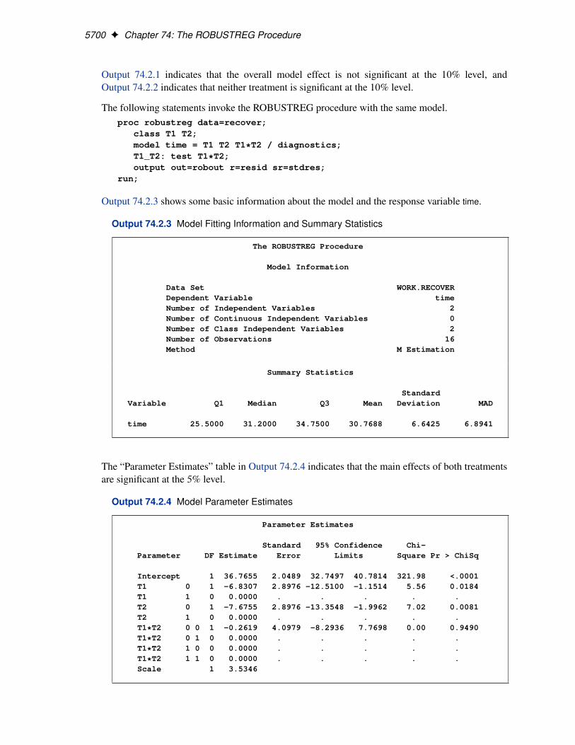
5700 F Chapter 74: The ROBUSTREG Procedure
Output 74.2.1 indicates that the overall model effect is not significant at the 10% level, andOutput 74.2.2 indicates that neither treatment is significant at the 10% level.
The following statements invoke the ROBUSTREG procedure with the same model.proc robustreg data=recover;
class T1 T2;model time = T1 T2 T1*T2 / diagnostics;T1_T2: test T1*T2;output out=robout r=resid sr=stdres;
run;
Output 74.2.3 shows some basic information about the model and the response variable time.
Output 74.2.3 Model Fitting Information and Summary Statistics
The ROBUSTREG Procedure
Model Information
Data Set WORK.RECOVERDependent Variable timeNumber of Independent Variables 2Number of Continuous Independent Variables 0Number of Class Independent Variables 2Number of Observations 16Method M Estimation
Summary Statistics
StandardVariable Q1 Median Q3 Mean Deviation MAD
time 25.5000 31.2000 34.7500 30.7688 6.6425 6.8941
The “Parameter Estimates” table in Output 74.2.4 indicates that the main effects of both treatmentsare significant at the 5% level.
Output 74.2.4 Model Parameter Estimates
Parameter Estimates
Standard 95% Confidence Chi-Parameter DF Estimate Error Limits Square Pr > ChiSq
Intercept 1 36.7655 2.0489 32.7497 40.7814 321.98 <.0001T1 0 1 -6.8307 2.8976 -12.5100 -1.1514 5.56 0.0184T1 1 0 0.0000 . . . . .T2 0 1 -7.6755 2.8976 -13.3548 -1.9962 7.02 0.0081T2 1 0 0.0000 . . . . .T1*T2 0 0 1 -0.2619 4.0979 -8.2936 7.7698 0.00 0.9490T1*T2 0 1 0 0.0000 . . . . .T1*T2 1 0 0 0.0000 . . . . .T1*T2 1 1 0 0.0000 . . . . .Scale 1 3.5346
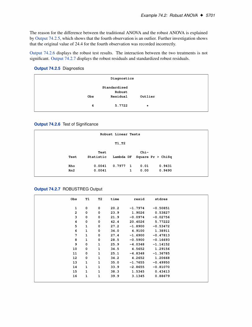
Example 74.2: Robust ANOVA F 5701
The reason for the difference between the traditional ANOVA and the robust ANOVA is explainedby Output 74.2.5, which shows that the fourth observation is an outlier. Further investigation showsthat the original value of 24.4 for the fourth observation was recorded incorrectly.
Output 74.2.6 displays the robust test results. The interaction between the two treatments is notsignificant. Output 74.2.7 displays the robust residuals and standardized robust residuals.
Output 74.2.5 Diagnostics
Diagnostics
StandardizedRobust
Obs Residual Outlier
4 5.7722 *
Output 74.2.6 Test of Significance
Robust Linear Tests
T1_T2
Test Chi-Test Statistic Lambda DF Square Pr > ChiSq
Rho 0.0041 0.7977 1 0.01 0.9431Rn2 0.0041 1 0.00 0.9490
Output 74.2.7 ROBUSTREG Output
Obs T1 T2 time resid stdres
1 0 0 20.2 -1.7974 -0.508512 0 0 23.9 1.9026 0.538273 0 0 21.9 -0.0974 -0.027564 0 0 42.4 20.4026 5.772225 1 0 27.2 -1.8900 -0.534726 1 0 34.0 4.9100 1.389117 1 0 27.4 -1.6900 -0.478138 1 0 28.5 -0.5900 -0.166939 0 1 25.9 -4.0348 -1.1415210 0 1 34.5 4.5652 1.2915611 0 1 25.1 -4.8348 -1.3678512 0 1 34.2 4.2652 1.2066813 1 1 35.0 -1.7655 -0.4995014 1 1 33.9 -2.8655 -0.8107015 1 1 38.3 1.5345 0.4341316 1 1 39.9 3.1345 0.88679
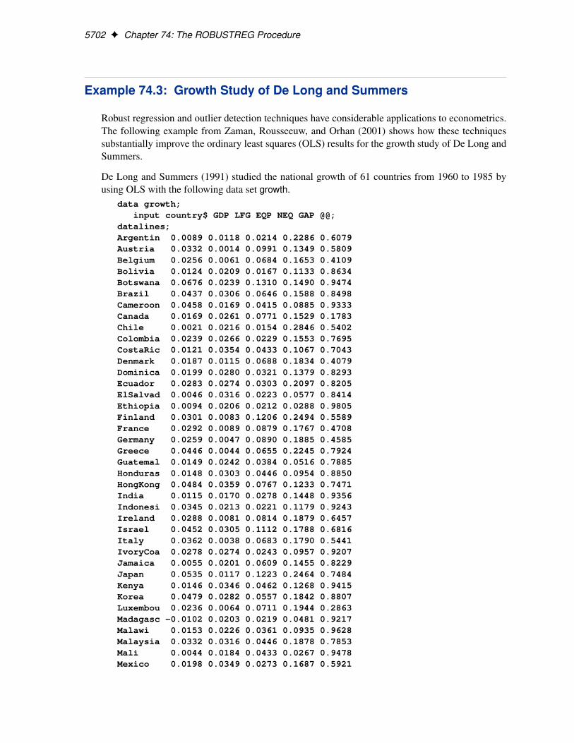
5702 F Chapter 74: The ROBUSTREG Procedure
Example 74.3: Growth Study of De Long and Summers
Robust regression and outlier detection techniques have considerable applications to econometrics.The following example from Zaman, Rousseeuw, and Orhan (2001) shows how these techniquessubstantially improve the ordinary least squares (OLS) results for the growth study of De Long andSummers.
De Long and Summers (1991) studied the national growth of 61 countries from 1960 to 1985 byusing OLS with the following data set growth.
data growth;input country$ GDP LFG EQP NEQ GAP @@;
datalines;Argentin 0.0089 0.0118 0.0214 0.2286 0.6079Austria 0.0332 0.0014 0.0991 0.1349 0.5809Belgium 0.0256 0.0061 0.0684 0.1653 0.4109Bolivia 0.0124 0.0209 0.0167 0.1133 0.8634Botswana 0.0676 0.0239 0.1310 0.1490 0.9474Brazil 0.0437 0.0306 0.0646 0.1588 0.8498Cameroon 0.0458 0.0169 0.0415 0.0885 0.9333Canada 0.0169 0.0261 0.0771 0.1529 0.1783Chile 0.0021 0.0216 0.0154 0.2846 0.5402Colombia 0.0239 0.0266 0.0229 0.1553 0.7695CostaRic 0.0121 0.0354 0.0433 0.1067 0.7043Denmark 0.0187 0.0115 0.0688 0.1834 0.4079Dominica 0.0199 0.0280 0.0321 0.1379 0.8293Ecuador 0.0283 0.0274 0.0303 0.2097 0.8205ElSalvad 0.0046 0.0316 0.0223 0.0577 0.8414Ethiopia 0.0094 0.0206 0.0212 0.0288 0.9805Finland 0.0301 0.0083 0.1206 0.2494 0.5589France 0.0292 0.0089 0.0879 0.1767 0.4708Germany 0.0259 0.0047 0.0890 0.1885 0.4585Greece 0.0446 0.0044 0.0655 0.2245 0.7924Guatemal 0.0149 0.0242 0.0384 0.0516 0.7885Honduras 0.0148 0.0303 0.0446 0.0954 0.8850HongKong 0.0484 0.0359 0.0767 0.1233 0.7471India 0.0115 0.0170 0.0278 0.1448 0.9356Indonesi 0.0345 0.0213 0.0221 0.1179 0.9243Ireland 0.0288 0.0081 0.0814 0.1879 0.6457Israel 0.0452 0.0305 0.1112 0.1788 0.6816Italy 0.0362 0.0038 0.0683 0.1790 0.5441IvoryCoa 0.0278 0.0274 0.0243 0.0957 0.9207Jamaica 0.0055 0.0201 0.0609 0.1455 0.8229Japan 0.0535 0.0117 0.1223 0.2464 0.7484Kenya 0.0146 0.0346 0.0462 0.1268 0.9415Korea 0.0479 0.0282 0.0557 0.1842 0.8807Luxembou 0.0236 0.0064 0.0711 0.1944 0.2863Madagasc -0.0102 0.0203 0.0219 0.0481 0.9217Malawi 0.0153 0.0226 0.0361 0.0935 0.9628Malaysia 0.0332 0.0316 0.0446 0.1878 0.7853Mali 0.0044 0.0184 0.0433 0.0267 0.9478Mexico 0.0198 0.0349 0.0273 0.1687 0.5921
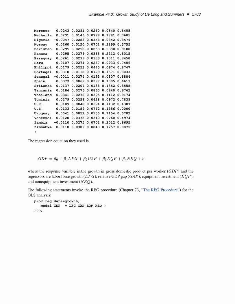
Example 74.3: Growth Study of De Long and Summers F 5703
Morocco 0.0243 0.0281 0.0260 0.0540 0.8405Netherla 0.0231 0.0146 0.0778 0.1781 0.3605Nigeria -0.0047 0.0283 0.0358 0.0842 0.8579Norway 0.0260 0.0150 0.0701 0.2199 0.3755Pakistan 0.0295 0.0258 0.0263 0.0880 0.9180Panama 0.0295 0.0279 0.0388 0.2212 0.8015Paraguay 0.0261 0.0299 0.0189 0.1011 0.8458Peru 0.0107 0.0271 0.0267 0.0933 0.7406Philippi 0.0179 0.0253 0.0445 0.0974 0.8747Portugal 0.0318 0.0118 0.0729 0.1571 0.8033Senegal -0.0011 0.0274 0.0193 0.0807 0.8884Spain 0.0373 0.0069 0.0397 0.1305 0.6613SriLanka 0.0137 0.0207 0.0138 0.1352 0.8555Tanzania 0.0184 0.0276 0.0860 0.0940 0.9762Thailand 0.0341 0.0278 0.0395 0.1412 0.9174Tunisia 0.0279 0.0256 0.0428 0.0972 0.7838U.K. 0.0189 0.0048 0.0694 0.1132 0.4307U.S. 0.0133 0.0189 0.0762 0.1356 0.0000Uruguay 0.0041 0.0052 0.0155 0.1154 0.5782Venezuel 0.0120 0.0378 0.0340 0.0760 0.4974Zambia -0.0110 0.0275 0.0702 0.2012 0.8695Zimbabwe 0.0110 0.0309 0.0843 0.1257 0.8875;
The regression equation they used is
GDP D ˇ0 C ˇ1LFG C ˇ2GAP C ˇ3EQP C ˇ4NEQC �
where the response variable is the growth in gross domestic product per worker (GDP ) and theregressors are labor force growth (LFG), relative GDP gap (GAP ), equipment investment (EQP ),and nonequipment investment (NEQ).
The following statements invoke the REG procedure (Chapter 73, “The REG Procedure”) for theOLS analysis:
proc reg data=growth;model GDP = LFG GAP EQP NEQ ;
run;
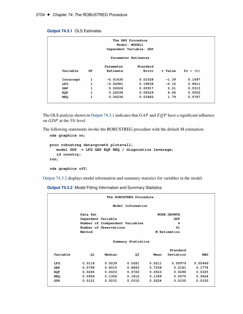
5704 F Chapter 74: The ROBUSTREG Procedure
Output 74.3.1 OLS Estimates
The REG ProcedureModel: MODEL1
Dependent Variable: GDP
Parameter Estimates
Parameter StandardVariable DF Estimate Error t Value Pr > |t|
Intercept 1 -0.01430 0.01028 -1.39 0.1697LFG 1 -0.02981 0.19838 -0.15 0.8811GAP 1 0.02026 0.00917 2.21 0.0313EQP 1 0.26538 0.06529 4.06 0.0002NEQ 1 0.06236 0.03482 1.79 0.0787
The OLS analysis shown in Output 74.3.1 indicates thatGAP andEQP have a significant influenceon GDP at the 5% level.
The following statements invoke the ROBUSTREG procedure with the default M estimation.ods graphics on;
proc robustreg data=growth plots=all;model GDP = LFG GAP EQP NEQ / diagnostics leverage;id country;
run;
ods graphics off;
Output 74.3.2 displays model information and summary statistics for variables in the model.
Output 74.3.2 Model Fitting Information and Summary Statistics
The ROBUSTREG Procedure
Model Information
Data Set WORK.GROWTHDependent Variable GDPNumber of Independent Variables 4Number of Observations 61Method M Estimation
Summary Statistics
StandardVariable Q1 Median Q3 Mean Deviation MAD
LFG 0.0118 0.0239 0.0281 0.0211 0.00979 0.00949GAP 0.5796 0.8015 0.8863 0.7258 0.2181 0.1778EQP 0.0265 0.0433 0.0720 0.0523 0.0296 0.0325NEQ 0.0956 0.1356 0.1812 0.1399 0.0570 0.0624GDP 0.0121 0.0231 0.0310 0.0224 0.0155 0.0150
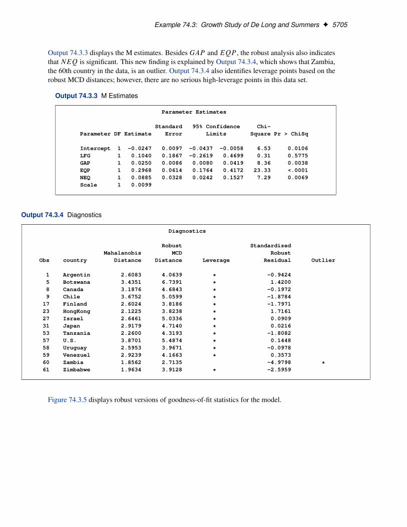
Example 74.3: Growth Study of De Long and Summers F 5705
Output 74.3.3 displays the M estimates. Besides GAP and EQP , the robust analysis also indicatesthatNEQ is significant. This new finding is explained by Output 74.3.4, which shows that Zambia,the 60th country in the data, is an outlier. Output 74.3.4 also identifies leverage points based on therobust MCD distances; however, there are no serious high-leverage points in this data set.
Output 74.3.3 M Estimates
Parameter Estimates
Standard 95% Confidence Chi-Parameter DF Estimate Error Limits Square Pr > ChiSq
Intercept 1 -0.0247 0.0097 -0.0437 -0.0058 6.53 0.0106LFG 1 0.1040 0.1867 -0.2619 0.4699 0.31 0.5775GAP 1 0.0250 0.0086 0.0080 0.0419 8.36 0.0038EQP 1 0.2968 0.0614 0.1764 0.4172 23.33 <.0001NEQ 1 0.0885 0.0328 0.0242 0.1527 7.29 0.0069Scale 1 0.0099
Output 74.3.4 Diagnostics
Diagnostics
Robust StandardizedMahalanobis MCD Robust
Obs country Distance Distance Leverage Residual Outlier
1 Argentin 2.6083 4.0639 * -0.94245 Botswana 3.4351 6.7391 * 1.42008 Canada 3.1876 4.6843 * -0.19729 Chile 3.6752 5.0599 * -1.8784
17 Finland 2.6024 3.8186 * -1.797123 HongKong 2.1225 3.8238 * 1.716127 Israel 2.6461 5.0336 * 0.090931 Japan 2.9179 4.7140 * 0.021653 Tanzania 2.2600 4.3193 * -1.808257 U.S. 3.8701 5.4874 * 0.144858 Uruguay 2.5953 3.9671 * -0.097859 Venezuel 2.9239 4.1663 * 0.357360 Zambia 1.8562 2.7135 -4.9798 *61 Zimbabwe 1.9634 3.9128 * -2.5959
Figure 74.3.5 displays robust versions of goodness-of-fit statistics for the model.
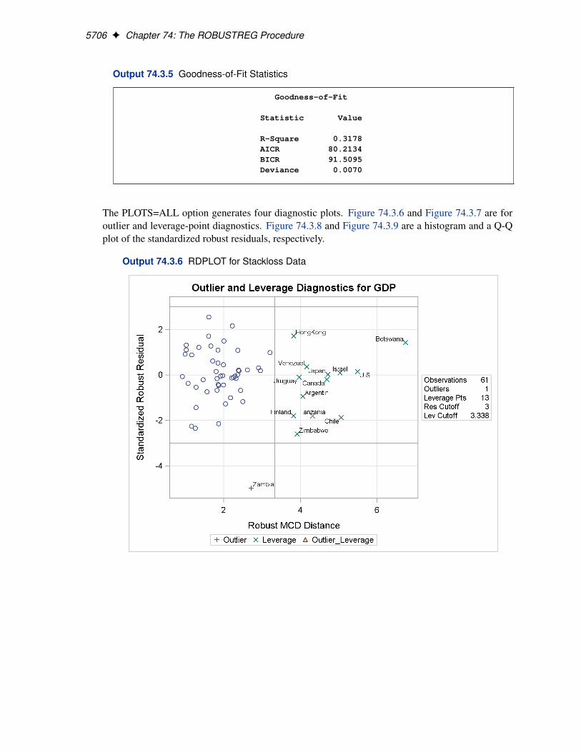
5706 F Chapter 74: The ROBUSTREG Procedure
Output 74.3.5 Goodness-of-Fit Statistics
Goodness-of-Fit
Statistic Value
R-Square 0.3178AICR 80.2134BICR 91.5095Deviance 0.0070
The PLOTS=ALL option generates four diagnostic plots. Figure 74.3.6 and Figure 74.3.7 are foroutlier and leverage-point diagnostics. Figure 74.3.8 and Figure 74.3.9 are a histogram and a Q-Qplot of the standardized robust residuals, respectively.
Output 74.3.6 RDPLOT for Stackloss Data
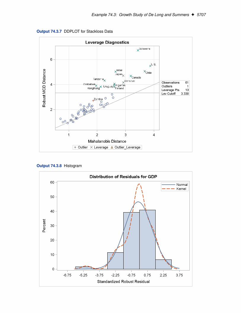
Example 74.3: Growth Study of De Long and Summers F 5707
Output 74.3.7 DDPLOT for Stackloss Data
Output 74.3.8 Histogram
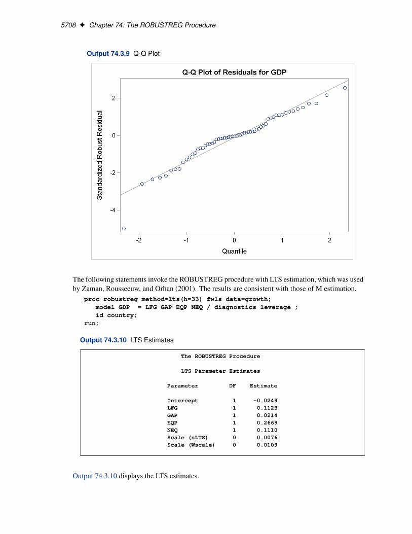
5708 F Chapter 74: The ROBUSTREG Procedure
Output 74.3.9 Q-Q Plot
The following statements invoke the ROBUSTREG procedure with LTS estimation, which was usedby Zaman, Rousseeuw, and Orhan (2001). The results are consistent with those of M estimation.
proc robustreg method=lts(h=33) fwls data=growth;model GDP = LFG GAP EQP NEQ / diagnostics leverage ;id country;
run;
Output 74.3.10 LTS Estimates
The ROBUSTREG Procedure
LTS Parameter Estimates
Parameter DF Estimate
Intercept 1 -0.0249LFG 1 0.1123GAP 1 0.0214EQP 1 0.2669NEQ 1 0.1110Scale (sLTS) 0 0.0076Scale (Wscale) 0 0.0109
Output 74.3.10 displays the LTS estimates.
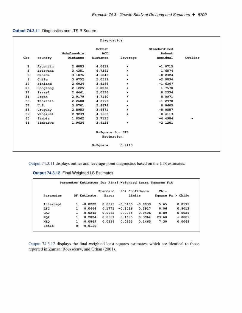
Example 74.3: Growth Study of De Long and Summers F 5709
Output 74.3.11 Diagnostics and LTS R Square
Diagnostics
Robust StandardizedMahalanobis MCD Robust
Obs country Distance Distance Leverage Residual Outlier
1 Argentin 2.6083 4.0639 * -1.07155 Botswana 3.4351 6.7391 * 1.65748 Canada 3.1876 4.6843 * -0.23249 Chile 3.6752 5.0599 * -2.0896
17 Finland 2.6024 3.8186 * -1.636723 HongKong 2.1225 3.8238 * 1.757027 Israel 2.6461 5.0336 * 0.233431 Japan 2.9179 4.7140 * 0.097153 Tanzania 2.2600 4.3193 * -1.297857 U.S. 3.8701 5.4874 * 0.060558 Uruguay 2.5953 3.9671 * -0.085759 Venezuel 2.9239 4.1663 * 0.411360 Zambia 1.8562 2.7135 -4.4984 *61 Zimbabwe 1.9634 3.9128 * -2.1201
R-Square for LTSEstimation
R-Square 0.7418
Output 74.3.11 displays outlier and leverage-point diagnostics based on the LTS estimates.
Output 74.3.12 Final Weighted LS Estimates
Parameter Estimates for Final Weighted Least Squares Fit
Standard 95% Confidence Chi-Parameter DF Estimate Error Limits Square Pr > ChiSq
Intercept 1 -0.0222 0.0093 -0.0405 -0.0039 5.65 0.0175LFG 1 0.0446 0.1771 -0.3026 0.3917 0.06 0.8013GAP 1 0.0245 0.0082 0.0084 0.0406 8.89 0.0029EQP 1 0.2824 0.0581 0.1685 0.3964 23.60 <.0001NEQ 1 0.0849 0.0314 0.0233 0.1465 7.30 0.0069Scale 0 0.0116
Output 74.3.12 displays the final weighted least squares estimates, which are identical to thosereported in Zaman, Rousseeuw, and Orhan (2001).
5710 F Chapter 74: The ROBUSTREG Procedure
References
Akaike, H. (1974), “A New Look at the Statistical Identification Model,” IEEE Trans. AutomatControl, 19, 716–723.
Brownlee, K.A. (1965), Statistical Theory and Methodology in Science and Engineering, 2nd ed.,New York: John Wiley & Sons, Inc.
Chen, C. (2002), “Robust Regression and Outlier Detection with the ROBUSTREG Procedure,”Proceedings of the Twenty-seventh Annual SAS Users Group International Conference, Cary, NC:SAS Institute Inc.
Chen, C. and Yin, G. (2002), “Computing the Efficiency and Tuning Constants for M-Estimation,”Proceedings of the Joint Statistical Meetings, 478–482.
Coleman, D. Holland, P., Kaden, N., Klema, V., and Peters, S.C. (1980), “A System of Subroutinesfor Iteratively Reweighted Least-Squares Computations,” ACM Transactions on Mathematical Soft-ware, 6, 327–336.
De Long, J.B. and Summers, L.H. (1991), “Equipment Investment and Economic Growth,” Quar-terly Journal of Economics, 106, 445–501.
Hampel, F. R., Ronchetti, E.M., Rousseeuw, P.J. and Stahel, W.A. (1986), Robust Statistics: TheApproach Based on Influence Functions, New York: John Wiley & Sons, Inc.
Hawkins, D.M., Bradu, D. and Kass, G.V. (1984), “Location of Several Outliers in Multiple Re-gression Data Using Elemental Sets,” Technometrics, 26, 197–208.
Holland, P. and Welsch, R. (1977), “Robust Regression Using Interactively Reweighted Least-Squares,” Commun. Statist. Theor. Meth., 6, 813–827.
Huber, P.J. (1973), “Robust Regression: Asymptotics, Conjectures and Monte Carlo,” Ann. Stat., 1,799–821.
Huber, P.J. (1981), Robust Statistics, New York: John Wiley & Sons, Inc.
Marazzi, A. (1993), Algorithm, Routines, and S Functions for Robust Statistics, Pacific Grove, CA:Wadsworth & Brooks/Cole.
Ronchetti, E. (1985), “Robust Model Selection in Regression,” Statistics and Probability Letters, 3,21–23.
Rousseeuw, P.J. (1984), “Least Median of Squares Regression,” Journal of the American StatisticalAssociation, 79, 871–880.
Rousseeuw, P.J. and Hubert, M. (1996), “Recent Development in PROGRESS,” ComputationalStatistics and Data Analysis, 21, 67–85.
Rousseeuw, P.J. and Leroy, A.M. (1987), Robust Regression and Outlier Detection, New York: JohnWiley & Sons, Inc.
References F 5711
Rousseeuw, P.J. and Van Driessen, K. (1999), “A Fast Algorithm for the Minimum CovarianceDeterminant Estimator,” Technometrics, 41, 212–223.
Rousseeuw, P.J. and Van Driessen, K. (2000), “An Algorithm for Positive-Breakdown RegressionBased on Concentration Steps,” Data Analysis: Scientific Modeling and Practical Application, ed.W. Gaul, O. Opitz, and M. Schader, New York: Springer-Verlag, 335–346.
Rousseeuw, P.J. and Yohai, V. (1984), “Robust Regression by Means of S Estimators,” in Robustand Nonlinear Time Series Analysis, ed. J. Franke, W. Härdle, and R.D. Martin, Lecture Notes inStatistics, 26, New York: Springer-Verlag, 256–274.
Ruppert, D. (1992), “Computing S Estimators for Regression and Multivariate Loca-tion/Dispersion,” Journal of Computational and Graphical Statistics, 1, 253–270.
Yohai V.J. (1987), “High Breakdown Point and High Efficiency Robust Estimates for Regression,”Annals of Statistics, 15, 642–656.
Yohai V.J., Stahel, W.A. and Zamar, R.H. (1991), “A Procedure for Robust Estimation and Inferencein Linear Regression,” in Stahel, W.A. and Weisberg, S.W., eds., Directions in Robust Statistics andDiagnostics, Part II, New York: Springer-Verlag.
Yohai, V.J. and Zamar, R.H. (1997), “Optimal Locally Robust M Estimate of Regression,” Journalof Statist. Planning and Inference, 64, 309–323.
Zaman, A., Rousseeuw, P.J., Orhan, M. (2001), “Econometric Applications of High-BreakdownRobust Regression Techniques,” Econometrics Letters, 71, 1–8.

Subject Index
computational resourcesROBUSTREG procedure, 5684
INEST= data setsROBUSTREG procedure, 5683
ODS graph namesROBUSTREG procedure, 5690
OUTEST= data setsROBUSTREG procedure, 5684
output table namesROBUSTREG procedure, 5685
ROBUSTREG procedure, 5642computational resources, 5684INEST= data sets, 5683ODS graph names, 5690OUTEST= data sets, 5684output table names, 5685

Syntax Index
ALPHA= optionMODEL statement (ROBUSTREG), 5663
BIASTEST optionPROC ROBUSTREG statement, 5660
BY statementROBUSTREG procedure, 5661
CHIF optionPROC ROBUSTREG statement, 5659, 5660
CLASS statementROBUSTREG procedure, 5662
CONVERGENCE optionPROC ROBUSTREG statement, 5657, 5661
CORRB optionMODEL statement (ROBUSTREG), 5663
COVARIANCE optionPROC ROBUSTREG statement, 5657, 5659PROC ROBUSTREG statement, 5660
COVB optionMODEL statement (ROBUSTREG), 5663
COVOUT optionPROC ROBUSTREG statement, 5654
CPUCOUNT optionPERFORMANCE statement
(ROBUSTREG), 5665CSTEP option
PROC ROBUSTREG statement, 5658CUTOFF option
MODEL statement (ROBUSTREG), 5663
DATA= optionPROC ROBUSTREG statement, 5654
DETAILS optionPERFORMANCE statement
(ROBUSTREG), 5665DIAGNOSTICS option
MODEL statement (ROBUSTREG), 5663
EFF optionPROC ROBUSTREG statement, 5659, 5661
FIADJUST optionPROC ROBUSTREG statement, 5658
FWLS= optionPROC ROBUSTREG statement, 5655
H optionPROC ROBUSTREG statement, 5659
ID statementROBUSTREG procedure, 5662
INEST= optionPROC ROBUSTREG statement, 5655
INITEST optionPROC ROBUSTREG statement, 5661
INITH optionPROC ROBUSTREG statement, 5661
ITPRINT optionMODEL statement, 5663PROC ROBUSTREG statement, 5655
K0 optionPROC ROBUSTREG statement, 5660, 5661
keyword= optionOUTPUT statement (ROBUSTREG), 5664
LEVERAGE keywordOUTPUT statement (ROBUSTREG), 5664
LEVERAGE optionMODEL statement, 5663
MAXITER= optionPROC ROBUSTREG statement
(ROBUSTREG), 5657, 5660, 5661METHOD= < ( options )>
PROC ROBUSTREG statement, 5657MODEL statement
ROBUSTREG procedure, 5662
NAMELEN= optionPROC ROBUSTREG statement, 5655
NBEST optionPROC ROBUSTREG statement, 5659
NOGOODFIT optionMODEL statement (ROBUSTREG), 5663
NOINT optionMODEL statement (ROBUSTREG), 5663
NOTHREADS optionPERFORMANCE statement
(ROBUSTREG), 5665NREP option
PROC ROBUSTREG statement, 5659, 5660
ORDER= optionPROC ROBUSTREG statement, 5655
OUT= optionOUTPUT statement (ROBUSTREG), 5664
OUTEST= option
PROC ROBUSTREG statement, 5655OUTLIER keyword
OUTPUT statement (ROBUSTREG), 5664OUTPUT statement
ROBUSTREG procedure, 5664
PERFORMANCE statementROBUSTREG procedure, 5665
PLOT= optionPROC ROBUSTREG statement, 5655
PREDICTED keywordOUTPUT statement (ROBUSTREG), 5664
PROC ROBUSTREG statement, seeROBUSTREG procedure
REFINE optionPROC ROBUSTREG statement, 5660
RESIDUAL keywordOUTPUT statement (ROBUSTREG), 5664
ROBUSTREG proceduresyntax, 5654
ROBUSTREG procedure, BY statement, 5661ROBUSTREG procedure, CLASS statement,
5662ROBUSTREG procedure, ID statement, 5662ROBUSTREG procedure, MODEL statement,
5662ALPHA= option, 5663CORRB option, 5663COVB option, 5663CUTOFF option, 5663DIAGNOSTICS option, 5663ITPRINT option, 5663LEVERAGE option, 5663NOGOODFIT option, 5663NOINT option, 5663SINGULAR= option, 5663
ROBUSTREG procedure, OUTPUT statement,5664
keyword= option, 5664LEVEARAGE keyword, 5664OUT= option, 5664OUTLIER keyword, 5664PREDICTED keyword, 5664RESIDUAL keyword, 5664SRESIDUAL keyword, 5664STD_ERR keyword, 5664XBETA keyword, 5664
ROBUSTREG procedure, PERFORMANCEstatement, 5665
CPUCOUNT option, 5665DETAILS option, 5665NOTHREADS option, 5665THREADS option, 5665
ROBUSTREG procedure, PROC ROBUSTREGstatement, 5654
BIASTEST option, 5660CHIF option, 5659, 5660CONVERGENCE option, 5657, 5661COVARIANCE option, 5657, 5659COVOUT option, 5654CSTEP option, 5658DATA= option, 5654EFF option, 5659, 5661FWLS= option, 5655H option, 5659IADJUST option, 5658INEST= option, 5655INITEST option, 5661INITH option, 5661ITPRINT option, 5655K0 option, 5660, 5661MAXITER= option, 5657, 5660, 5661NAMELEN= option, 5655NBEST option, 5659NREP option, 5659, 5660ORDER= option, 5655OUTEST= option, 5655PLOT= option, 5655REFINE option, 5660SCALE option, 5658SUBANALYSIS option, 5659SUBGROUPSIZE option, 5659SUBSETSIZE option, 5660TOLERANCE option, 5660WEIGHTFUNCTION option, 5658
ROBUSTREG procedure, TEST statement, 5665ROBUSTREG procedure, WEIGHT statement,
5666ROBUSTREG procedure,PROC ROBUSTREG
statementCOVARIANCE option, 5660SEED option, 5657
SCALE optionPROC ROBUSTREG statement, 5658
SEED optionPROC ROBUSTREG statement
(ROBUSTREG), 5657SINGULAR= option
MODEL statement (ROBUSTREG), 5663SRESIDUAL keyword
OUTPUT statement (ROBUSTREG), 5664STD_ERR keyword
OUTPUT statement (ROBUSTREG), 5664SUBANALYSIS option
PROC ROBUSTREG statement, 5659SUBGROUPSIZE option
PROC ROBUSTREG statement, 5659SUBSETSIZE option
PROC ROBUSTREG statement, 5660
TEST statementROBUSTREG procedure, 5665
THREADS optionPERFORMANCE statement
(ROBUSTREG), 5665TOLERANCE option
PROC ROBUSTREG statement, 5660
WEIGHT statementROBUSTREG procedure, 5666
WEIGHTFUNCTIONT optionPROC ROBUSTREG statement, 5658
XBETA keywordOUTPUT statement (ROBUSTREG), 5664


Your Turn
We welcome your feedback.
� If you have comments about this book, please send them [email protected]. Include the full title and page numbers (ifapplicable).
� If you have comments about the software, please send them [email protected].


SAS® Publishing Delivers!Whether you are new to the work force or an experienced professional, you need to distinguish yourself in this rapidly changing and competitive job market. SAS® Publishing provides you with a wide range of resources to help you set yourself apart. Visit us online at support.sas.com/bookstore.
SAS® Press Need to learn the basics? Struggling with a programming problem? You’ll find the expert answers that you need in example-rich books from SAS Press. Written by experienced SAS professionals from around the world, SAS Press books deliver real-world insights on a broad range of topics for all skill levels.
s u p p o r t . s a s . c o m / s a s p r e s sSAS® Documentation To successfully implement applications using SAS software, companies in every industry and on every continent all turn to the one source for accurate, timely, and reliable information: SAS documentation. We currently produce the following types of reference documentation to improve your work experience:
• Onlinehelpthatisbuiltintothesoftware.• Tutorialsthatareintegratedintotheproduct.• ReferencedocumentationdeliveredinHTMLandPDF– free on the Web. • Hard-copybooks.
s u p p o r t . s a s . c o m / p u b l i s h i n gSAS® Publishing News Subscribe to SAS Publishing News to receive up-to-date information about all new SAS titles, author podcasts, and new Web site features via e-mail. Complete instructions on how to subscribe, as well as access to past issues, are available at our Web site.
s u p p o r t . s a s . c o m / s p n
SAS and all other SAS Institute Inc. product or service names are registered trademarks or trademarks of SAS Institute Inc. in the USA and other countries. ® indicates USA registration. Otherbrandandproductnamesaretrademarksoftheirrespectivecompanies.©2009SASInstituteInc.Allrightsreserved.518177_1US.0109