Saran Janjira and Rathanawan Magaraphan* · Saran Janjira and Rathanawan Magaraphan* The Petroleum and Petrochemical College, Chulalongkorn University, ... was taken from the 1997

30 Int. J. Environment and Pollution, Vol. 29, Nos. 1/2/3, 2007

Copyright © 2007 Inderscience Enterprises Ltd.

Simultaneous treatment of environmental and financial risk in process design

Saran Janjira and Rathanawan Magaraphan* The Petroleum and Petrochemical College, Chulalongkorn University, Bangkok, 10330, Thailand E-mail: [email protected] E-mail: [email protected] Website: www.ppc.chula.ac.th *Corresponding author

Miguel J. Bagajewicz School of Chemical Engineering and Materials Science, University of Oklahoma, Norman, Okalahoma, 73019, USA Website: http://www.ou.edu/class/che-design/

Abstract: In this paper, we propose a new measure for environmental risk and discuss a way of considering it simultaneously with financial risk. Instead of using single numbers to define environmental risk, we propose to use the cumulative probability of emissions, similarly to the cumulative distributions of profit used for financial risk. We also propose to use a risk surface as a generalisation of the known one-dimensional risk representation through cumulative probabilities and we show how different risks can be handled with this scheme. As an example, we use a catalytic reforming unit where CO2 and benzene emissions are of concern.

Keywords: process design; reforming process; risk management; financial risk; environmental risk; design under uncertainty.

Reference to this paper should be made as follows: Janjira, S., Magaraphan, R. and Bagajewicz, M.J. (2007) ‘Simultaneous treatment of environmental and financial risk in process design’, Int. J. Environment and Pollution, Vol. 29, Nos. 1/2/3, pp.30–46.

Biographical notes: Saran Janjira graduated from Chulalongkorn University. He received MS in Petroleum Technology in 2004 and BE in Chemical Engineering in 2002. He worked for Shell Company in Thailand during 2004 and early 2005. He is looking forward to continue PhD study.

Rathanawan Magaraphan is an Associate Professor in Polymer Science and Engineering at the Petroleum and Petrochemical College, Chulalongkorn University, Bangkok. She received her PhD in Polymer Science from the University of Akron in 1996 together with MSc in Engineering (Engineering Management) and in 1993, MSc in Engineering (Polymer Engineering) from the same university. Her BSc in Chemical Engineering was given in 1988 from Chulalongkorn University. She currently works on topics in polymer processing, financial and environmental risk management.

Simultaneous treatment of environmental and financial risk 31

Miguel J. Bagajewicz is a Professor of Chemical Engineering at the University of Oklahoma. He received his PhD from the California Institute of Technology in 1987. He has published extensively in the area of water management, energy efficiency in processes, instrumentation network design and lately on financial risk in process design and operations as well as in investment planning.

1 Introduction

In recent years, environmental impact limitations have been added as goals to the traditional profit maximisation in process design. This has been discussed in detail by several papers (Hoppel et al., 1992; Mallick et al., 1996; Chang and Hwang, 1996; Lim et al., 1999; Dantus and High, 1999; Yang and Shi, 2000; Alexander et al., 2000; Chen et al., 2002; Chakraborty and Linninger, 2002, 2003), and at least one book (Allen and Shonnard, 2002). The new emerging trend is therefore one of treating both environmental impact and profit simultaneously as conflicting objectives.

Environmental impact has been assessed using measures such as life cycle analysis (Henn and Fava, 1992; Lankey and Anastas, 2002), the sustainable process index (Krotscheck and Narodoslawski, 1996) and, the environmental impact index of each chemical (Mallick et al., 1996; Dantus and High, 1999). Dantus and High (1999) used a stochastic optimisation framework, based on simulations and a simulated annealing scheme. Reaction constants, environmental impact indices, utility prices and a release factor for non-waste streams were considered uncertain. Throughput changes as well as a time horizon were not considered.

In turn, environmental risk was defined differently. Arnold, Froiman and Blouin (Chapter 2 of Allen and Shonnard, 2002) define environmental risk as “the probability that a substance or a situation will produce harm under specific conditions”. The definition goes on to add: “Risk is a combination of two factors: the probability that an adverse event will occur and the consequences of the adverse event”. The definition was taken from the 1997 US Presidential/Congressional Commission on Risk Assessment and Risk Management Vol. 1. Because the above definition is not properly linked to uncertainty, an alternative definition, similar to that of financial risk is needed.

In engineering, financial risk is defined by a cumulative probability distribution of profit (Barbaro and Bagajewicz, 2004), or through measures like downside risk (Eppen et al., 1989). In finances, especially in stock portfolio optimisation, financial risk is associated to volatility of the profit distribution through a variety of metrics like variance or Value at Risk (VaR) (Jorion, 2000). Recently, Barbaro and Bagajewicz (2004) posed the risk management problem in the framework of two-stage stochastic programming.

In this paper, we introduce an alternative definition of risk, associated to process design and we discuss the simultaneous management of financial and environmental risk. We first define the structure of the problem from the conceptual point of view. Next, we review financial risk concepts and later we introduce our definition of environmental risk. Then, we illustrate how these two risks can be managed simultaneously. As an example, we use a catalytic reforming process, for which the plant capacity, the heat exchanger network, and reactor temperature are determined.

32 S. Janjira, R. Magaraphan and M.J. Bagajewicz

2 Problem statement

The following optimisation problem represents the classical single criteria design paradigm dominated by cost minimisation.

Minimise s.t.

Expected cost

Material and energy balancesProperty calculation equationsEquipment design equationsContainment of expected values of environmental impactContainment of risk (environmental

and financial).

(1)

The problem, however is a particular case of a multicriteria optimisation formulation, used by Dantus and High (1999) and Steffens et al. (1999) (who did not add risk), which can be sated as follows:

Minimise s.t.

.

Expected cost, Expected environmental impact indices,

Material and energy balancesProperty calculation equationsEquipment design equations

( )Risks both

(2)

The above is the conceptual framework we want to adopt, with the added feature that we also re-define environmental risk. Our purpose is to illustrate conceptually without resorting to complex algorithms how this framework can be used.

3 Financial risk

Financial risk is defined as the probability that the profit (or any other utility function) of a design x will be lower than a certain target value Ω (Barbaro and Bagajewicz, 2004):

FRisk(x, Ω) = PProfit(x) ≤ Ω. (3)

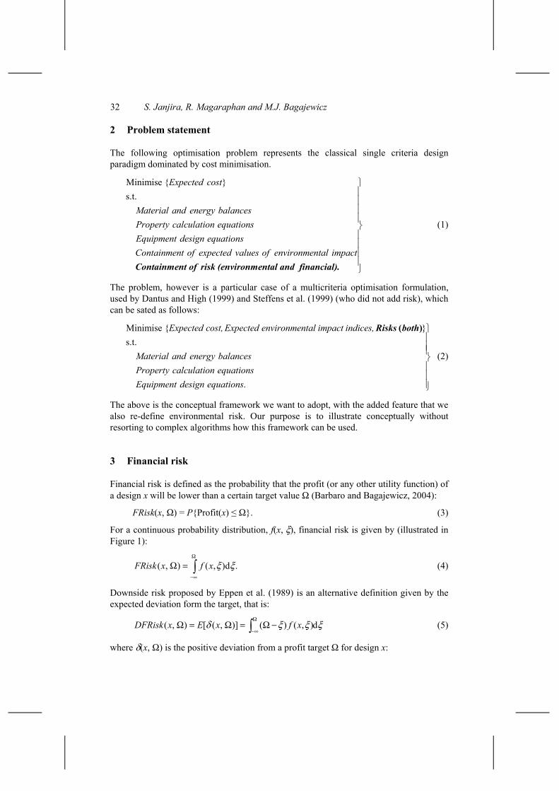
For a continuous probability distribution, f(x, ξ), financial risk is given by (illustrated in Figure 1):

( , ) ( , )d .FRisk x f x ξ ξΩ

−∞

Ω = ∫ (4)

Downside risk proposed by Eppen et al. (1989) is an alternative definition given by the expected deviation form the target, that is:

( , ) [ ( , )] ( ) ( , )dDFRisk x E x f xδ ξ ξ ξΩ

−∞Ω = Ω = Ω−∫ (5)

where δ(x, Ω) is the positive deviation from a profit target Ω for design x:


Profit( ) if Profit( )( , )

0 Otherwise.x x

xδΩ− < Ω

Ω =

(6)

Figure 1 Definition of risk

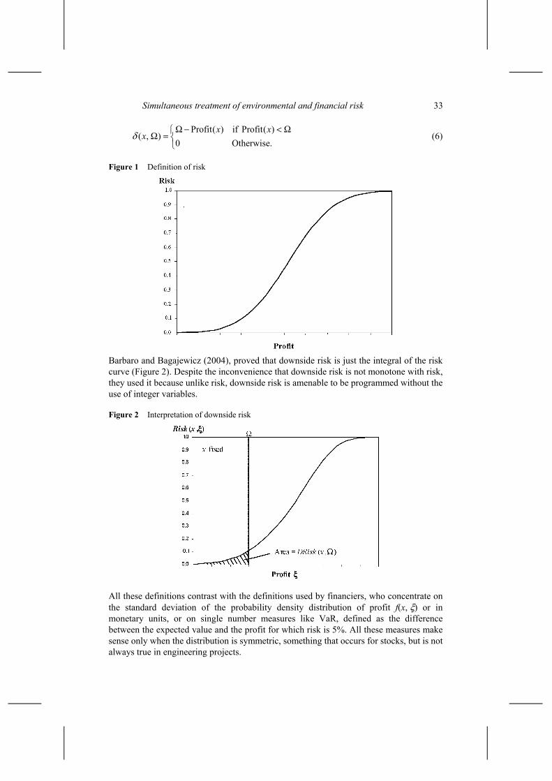
Barbaro and Bagajewicz (2004), proved that downside risk is just the integral of the risk curve (Figure 2). Despite the inconvenience that downside risk is not monotone with risk, they used it because unlike risk, downside risk is amenable to be programmed without the use of integer variables.

Figure 2 Interpretation of downside risk

All these definitions contrast with the definitions used by financiers, who concentrate on the standard deviation of the probability density distribution of profit f(x, ξ) or in monetary units, or on single number measures like VaR, defined as the difference between the expected value and the profit for which risk is 5%. All these measures make sense only when the distribution is symmetric, something that occurs for stocks, but is not always true in engineering projects.


4 Environmental risk

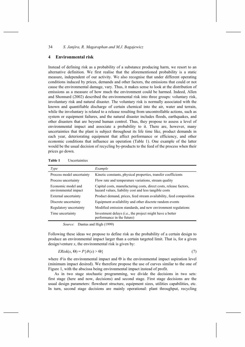
Instead of defining risk as a probability of a substance producing harm, we resort to an alternative definition. We first realise that the aforementioned probability is a static measure, independent of our activity. We also recognise that under different operating conditions induced by prices, demands and other factors, the emissions that could or not cause the environmental damage, vary. Thus, it makes sense to look at the distribution of emissions as a measure of how much the environment could be harmed. Indeed, Allen and Shonnard (2002) described the environmental risk into three groups: voluntary risk, involuntary risk and natural disaster. The voluntary risk is normally associated with the known and quantifiable discharge of certain chemical into the air, water and terrain, while the involuntary is related to a release resulting from uncontrollable actions, such as system or equipment failures, and the natural disaster includes floods, earthquakes, and other disasters that are beyond human control. Thus, they propose to assess a level of environmental impact and associate a probability to it. There are, however, many uncertainties that the plant is subject throughout its life time like, product demands in each year, deteriorating equipment that affect performance or efficiency, and other economic conditions that influence an operation (Table 1). One example of the latter would be the usual decision of recycling by-products to the feed of the process when their prices go down.

Table 1 Uncertainties

Type Example

Process model uncertainty Kinetic constants, physical properties, transfer coefficients Process uncertainty Flow rate and temperature variations, stream quality Economic model and environmental impact

Capital costs, manufacturing costs, direct costs, release factors, hazard values, liability cost and less tangible costs

External uncertainty Product demand, prices, feed stream availability, feed composition Discrete uncertainty Equipment availability and other discrete random events Regulatory uncertainty Modified emission standards, and new environment regulations Time uncertainty Investment delays (i.e., the project might have a better

performance in the future)

Source: Dantus and High (1999)

Following these ideas we propose to define risk as the probability of a certain design to produce an environmental impact larger than a certain targeted limit. That is, for a given design/venture x, the environmental risk is given by:

ERisk(x, Θ) = Pθ (x) > Θ (7)

where θ is the environmental impact and Θ is the environmental impact aspiration level (minimum impact desired). We therefore propose the use of curves similar to the one of Figure 1, with the abscissa being environmental impact instead of profit.

As in two stage stochastic programming, we divide the decisions in two sets: first stage (here and now, decisions) and second stage. First stage decisions are the usual design parameters: flowsheet structure, equipment sizes, utilities capabilities, etc. In turn, second stage decisions are mainly operational: plant throughput, recycling


of by-products, product qualities, maintenance actions, etc. These are a function of the actual product demand and the efficiency of the equipment, which as said, can deteriorate through time.

Since the reduction of environmental impact is conflicting with profit most of the time, the two need to be managed. We now illustrate these concepts.

5 Example: catalytic reforming process

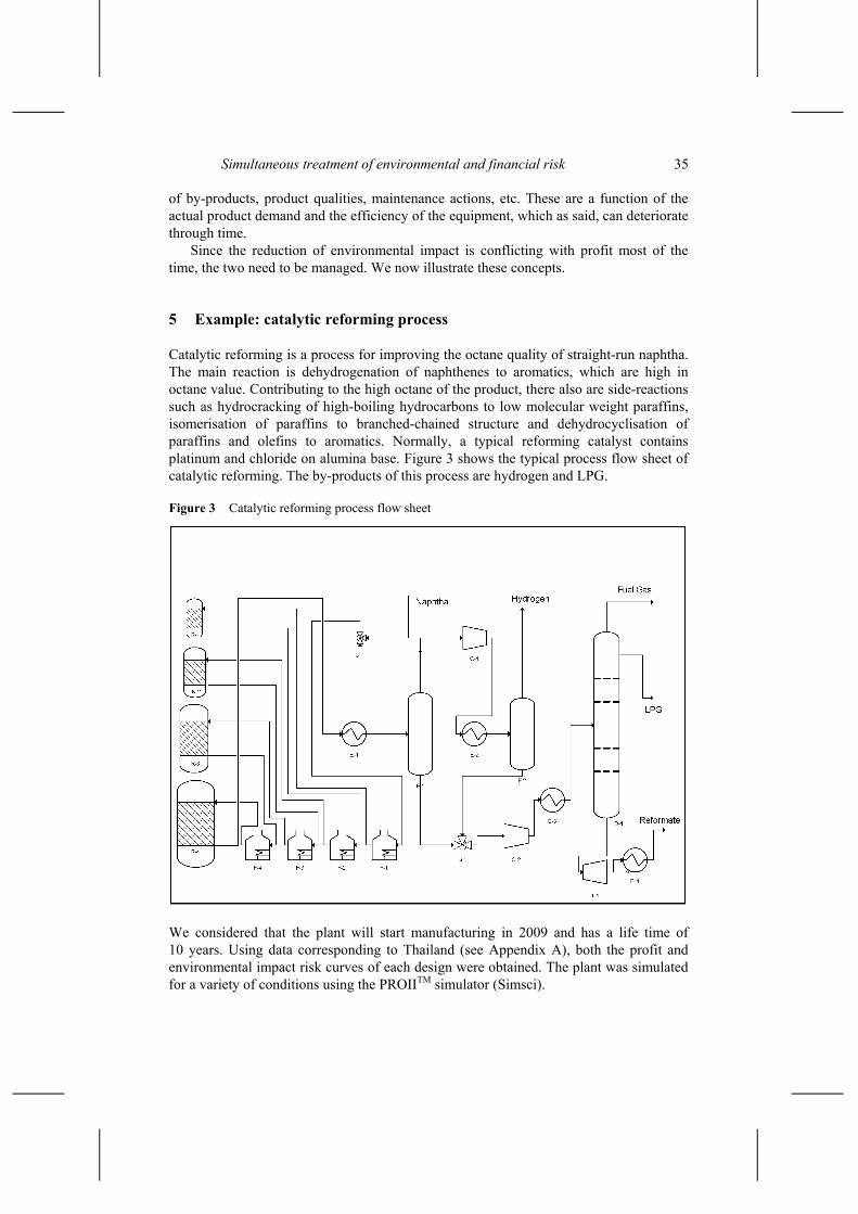
Catalytic reforming is a process for improving the octane quality of straight-run naphtha. The main reaction is dehydrogenation of naphthenes to aromatics, which are high in octane value. Contributing to the high octane of the product, there also are side-reactions such as hydrocracking of high-boiling hydrocarbons to low molecular weight paraffins, isomerisation of paraffins to branched-chained structure and dehydrocyclisation of paraffins and olefins to aromatics. Normally, a typical reforming catalyst contains platinum and chloride on alumina base. Figure 3 shows the typical process flow sheet of catalytic reforming. The by-products of this process are hydrogen and LPG.

Figure 3 Catalytic reforming process flow sheet

We considered that the plant will start manufacturing in 2009 and has a life time of 10 years. Using data corresponding to Thailand (see Appendix A), both the profit and environmental impact risk curves of each design were obtained. The plant was simulated for a variety of conditions using the PROIITM simulator (Simsci).


To find the overall environmental impact, the amount of carbon dioxide and benzene are combined to represent the impact for each design. In this work, benzene was valued to have 3.5 times larger impact than carbon dioxide, due to higher concern in the carcinogenic hazardous effect. Hence, the formula for environmental impact is:

EI = 3.5 × benzene production + carbon dioxide production. (8)

One can of course, use any other environmental impact measure, including global warming impact, and many others (Allen and Shonnard, 2002).

The kinetic models for catalytic reforming were first proposed by Krane et al. (1959). Then the important improvement of model was carried out by Jenkins and Stephen (1980) and Aguilar-Rodriguez and Ancheyta-Juarez (1994). They added a correlation to Krane’s models. We used the Jenkins and Stephen (1980) model with activation energies taken from Henningen and Bundgard (1970).

The separation processes were simulated in PRO IITM and two different heat recovery options were evaluated: a straight pinch design method with HRAT = 10°C and an alternative network resulted from the identification of loops and the application of the procedure for reducing the number of exchangers. We call this last design the ‘energy-relaxed’ design.

The reactor temperature is indicator of severity. Higher severity means lower reformate yield but higher quality of reformate (lower octane number). Besides, the cracked hydrocarbons amount increases at high severity. Also at higher temperatures, the level of aromatics is higher. The benzene produced was calculated by means of kinetic reaction model and finally, the CO2 release was obtained from furnace duty. Appendix 1 summarises the main results.

We chose one capacity (14 kbd) and two reactor temperatures (495°C and 501°C) as basic designs. This results in four alternatives (high/low temperature and pinch/energy-relaxed heat recovery). The costs for the four basic designs were scaled up for other capacities (20 and 26 kbd) using a scaling factor of 0.6 (Table A1). These capacities were carefully chosen after studying the projected gasoline demand and naphtha supply data. The four different designs are summarised in Table 2 and Figures A1 and A2 in Appendix A.

Table 2 Type of designs considered

Type of design Heat exchanger network Reacting temperature (°C) a Pinch design 495 b Pinch design 501 c Energy-relaxed 495 d Energy-relaxed 501

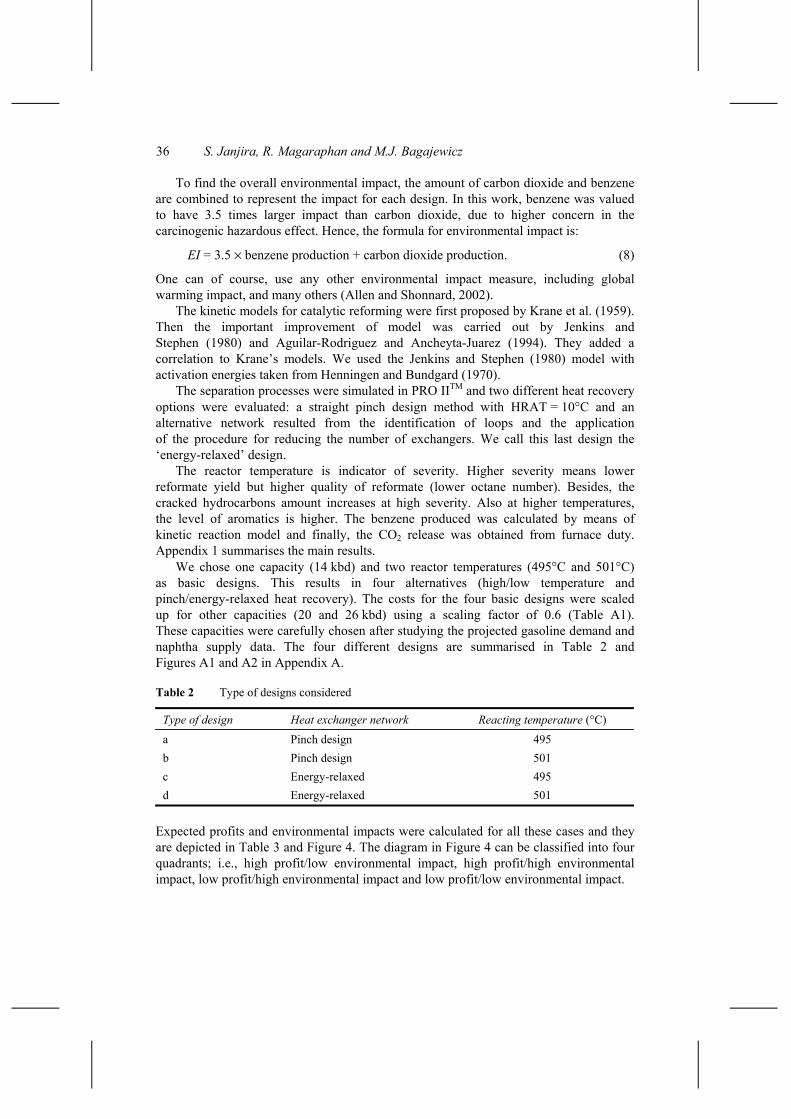
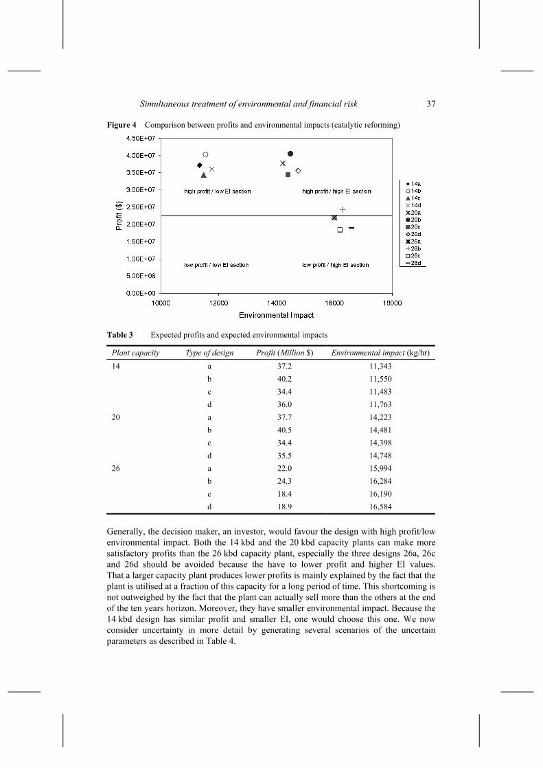
Expected profits and environmental impacts were calculated for all these cases and they are depicted in Table 3 and Figure 4. The diagram in Figure 4 can be classified into four quadrants; i.e., high profit/low environmental impact, high profit/high environmental impact, low profit/high environmental impact and low profit/low environmental impact.


Figure 4 Comparison between profits and environmental impacts (catalytic reforming)

Table 3 Expected profits and expected environmental impacts

Plant capacity Type of design Profit (Million $) Environmental impact (kg/hr) 14 a 37.2 11,343 b 40.2 11,550 c 34.4 11,483 d 36.0 11,763 20 a 37.7 14,223 b 40.5 14,481 c 34.4 14,398 d 35.5 14,748 26 a 22.0 15,994 b 24.3 16,284 c 18.4 16,190 d 18.9 16,584

Generally, the decision maker, an investor, would favour the design with high profit/low environmental impact. Both the 14 kbd and the 20 kbd capacity plants can make more satisfactory profits than the 26 kbd capacity plant, especially the three designs 26a, 26c and 26d should be avoided because the have to lower profit and higher EI values. That a larger capacity plant produces lower profits is mainly explained by the fact that the plant is utilised at a fraction of this capacity for a long period of time. This shortcoming is not outweighed by the fact that the plant can actually sell more than the others at the end of the ten years horizon. Moreover, they have smaller environmental impact. Because the 14 kbd design has similar profit and smaller EI, one would choose this one. We now consider uncertainty in more detail by generating several scenarios of the uncertain parameters as described in Table 4.


Table 4 Uncertain parameters

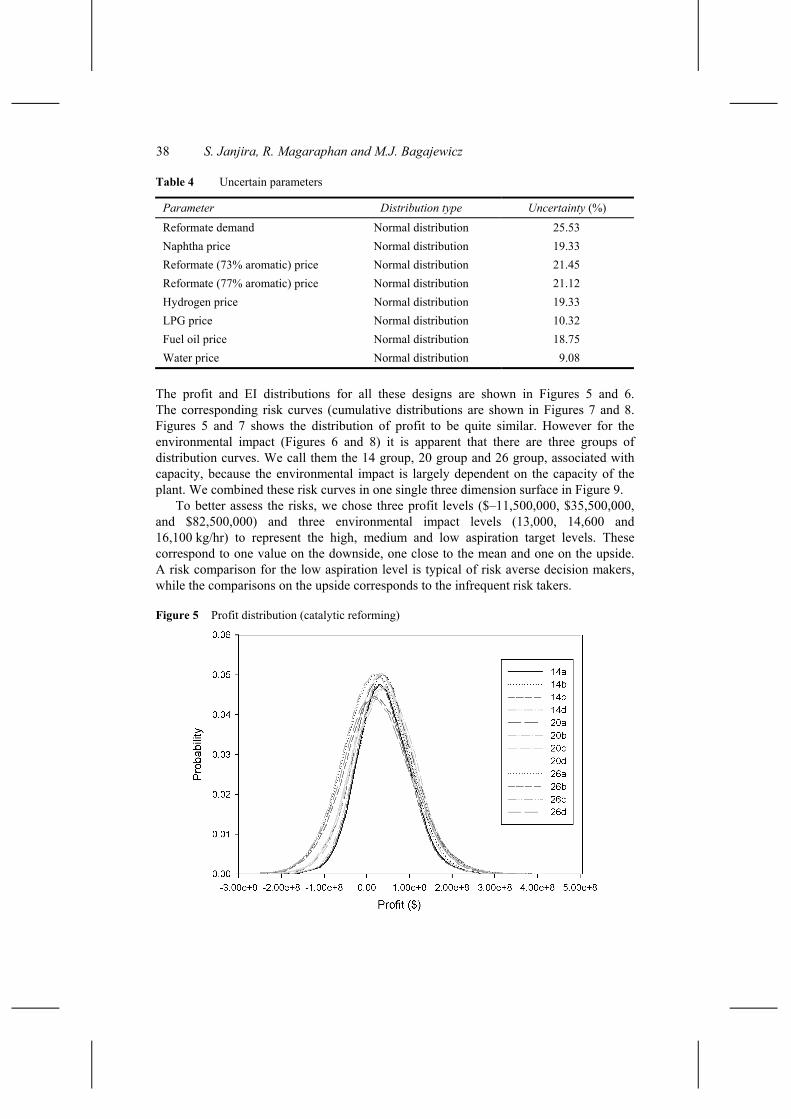
Parameter Distribution type Uncertainty (%) Reformate demand Normal distribution 25.53 Naphtha price Normal distribution 19.33 Reformate (73% aromatic) price Normal distribution 21.45 Reformate (77% aromatic) price Normal distribution 21.12 Hydrogen price Normal distribution 19.33 LPG price Normal distribution 10.32 Fuel oil price Normal distribution 18.75 Water price Normal distribution 9.08

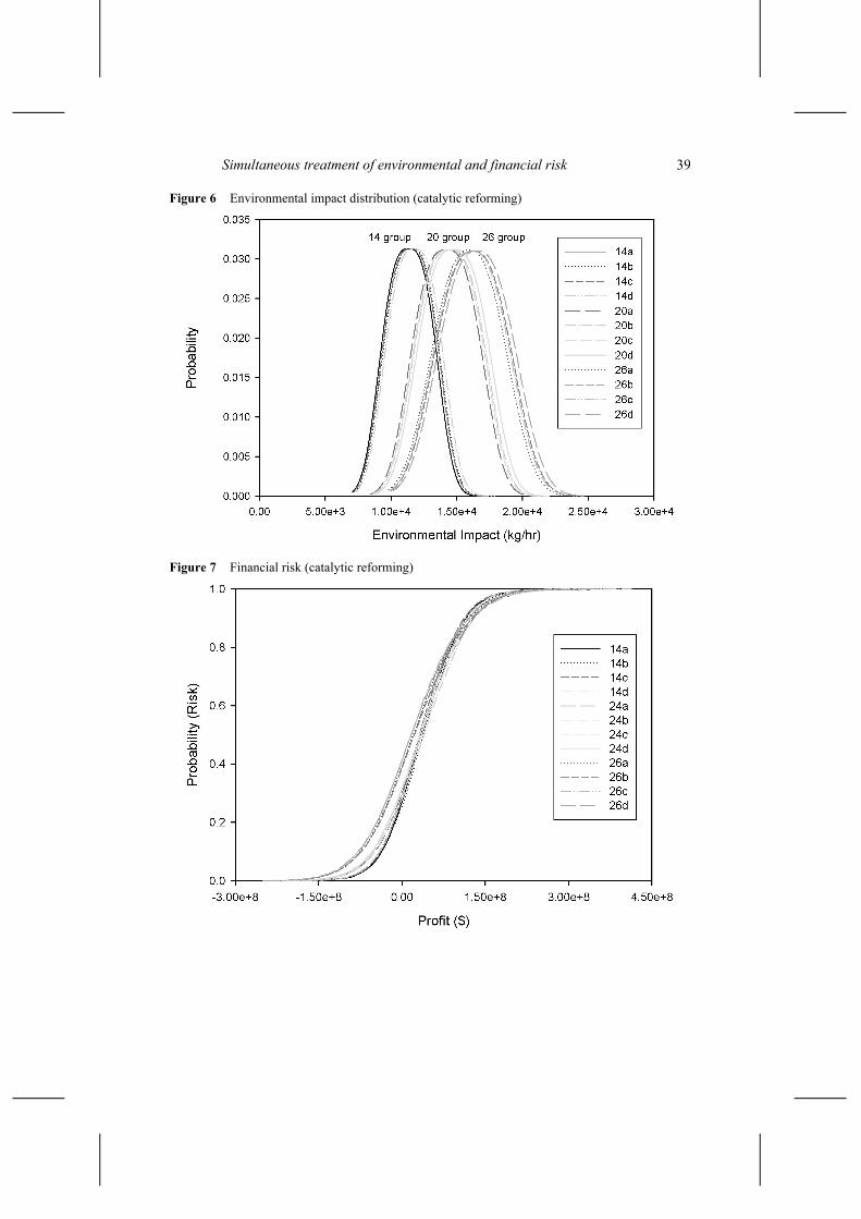
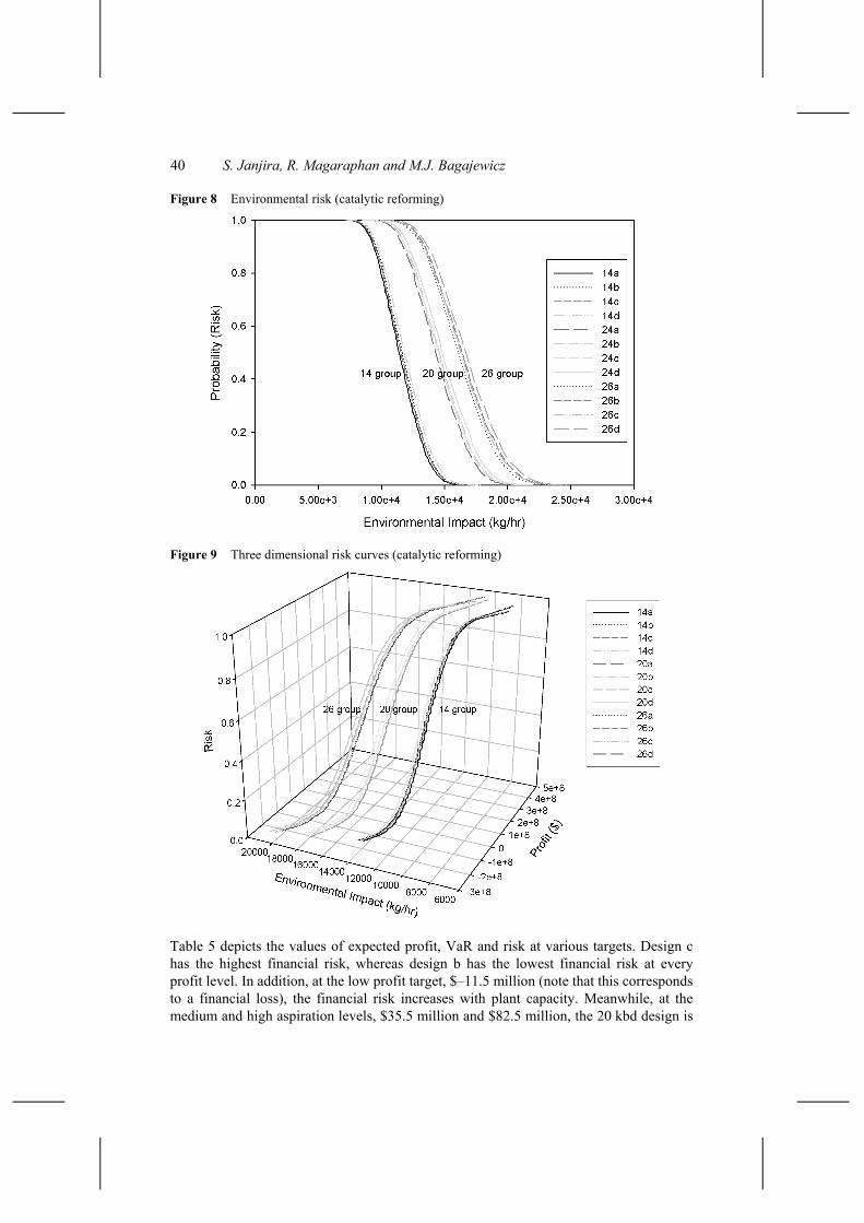
The profit and EI distributions for all these designs are shown in Figures 5 and 6. The corresponding risk curves (cumulative distributions are shown in Figures 7 and 8. Figures 5 and 7 shows the distribution of profit to be quite similar. However for the environmental impact (Figures 6 and 8) it is apparent that there are three groups of distribution curves. We call them the 14 group, 20 group and 26 group, associated with capacity, because the environmental impact is largely dependent on the capacity of the plant. We combined these risk curves in one single three dimension surface in Figure 9.

To better assess the risks, we chose three profit levels ($–11,500,000, $35,500,000, and $82,500,000) and three environmental impact levels (13,000, 14,600 and 16,100 kg/hr) to represent the high, medium and low aspiration target levels. These correspond to one value on the downside, one close to the mean and one on the upside. A risk comparison for the low aspiration level is typical of risk averse decision makers, while the comparisons on the upside corresponds to the infrequent risk takers.

Figure 5 Profit distribution (catalytic reforming)


Figure 6 Environmental impact distribution (catalytic reforming)

Figure 7 Financial risk (catalytic reforming)


Figure 8 Environmental risk (catalytic reforming)

Figure 9 Three dimensional risk curves (catalytic reforming)

Table 5 depicts the values of expected profit, VaR and risk at various targets. Design c has the highest financial risk, whereas design b has the lowest financial risk at every profit level. In addition, at the low profit target, $–11.5 million (note that this corresponds to a financial loss), the financial risk increases with plant capacity. Meanwhile, at the medium and high aspiration levels, $35.5 million and $82.5 million, the 20 kbd design is


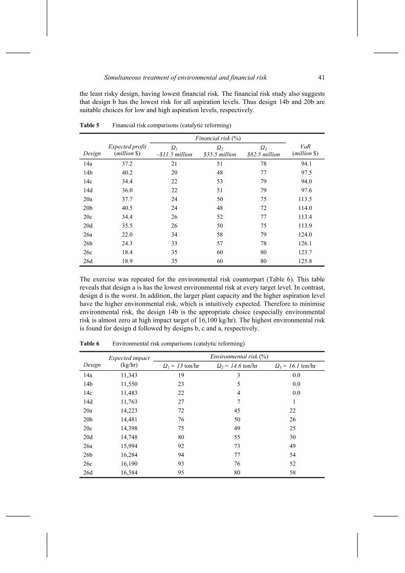
the least risky design, having lowest financial risk. The financial risk study also suggests that design b has the lowest risk for all aspiration levels. Thus design 14b and 20b are suitable choices for low and high aspiration levels, respectively.

Table 5 Financial risk comparisons (catalytic reforming)

Financial risk (%)

Design Expected profit

(million $) Ω1

–$11.5 million Ω2

$35.5 million Ω3

$82.5 million VaR

(million $)

14a 37.2 21 51 78 94.1 14b 40.2 20 48 77 97.5 14c 34.4 22 53 79 94.0 14d 36.0 22 51 79 97.6 20a 37.7 24 50 75 113.5 20b 40.5 24 48 72 114.0 20c 34.4 26 52 77 113.4 20d 35.5 26 50 75 113.9 26a 22.0 34 58 79 124.0 26b 24.3 33 57 78 126.1 26c 18.4 35 60 80 123.7 26d 18.9 35 60 80 125.8

The exercise was repeated for the environmental risk counterpart (Table 6). This table reveals that design a is has the lowest environmental risk at every target level. In contrast, design d is the worst. In addition, the larger plant capacity and the higher aspiration level have the higher environmental risk, which is intuitively expected. Therefore to minimise environmental risk, the design 14b is the appropriate choice (especially environmental risk is almost zero at high impact target of 16,100 kg/hr). The highest environmental risk is found for design d followed by designs b, c and a, respectively.

Table 6 Environmental risk comparisons (catalytic reforming)

Environmental risk (%) Design

Expected impact (kg/hr) Ω1 = 13 ton/hr Ω2 = 14.6 ton/hr Ω3 = 16.1 ton/hr

14a 11,343 19 3 0.0 14b 11,550 23 5 0.0 14c 11,483 22 4 0.0 14d 11,763 27 7 1 20a 14,223 72 45 22 20b 14,481 76 50 26 20c 14,398 75 49 25 20d 14,748 80 55 30 26a 15,994 92 73 49 26b 16,284 94 77 54 26c 16,190 93 76 52 26d 16,584 95 80 58


Consider designs 14b and 20b, those having the highest expected profits: design 14b has a slightly lower profit, but also a lower risk at low expectations (the region that a risk averse investor looks at). This is better seen by comparing the values of VaR. Moreover, design 14b produces much less environmental impact than design 20b for any aspiration levels. It is clear that 14b should be chosen.

6 Conclusion

In this paper, we introduced a new definition of environmental risk. This risk is defined by the cumulative probability of emissions associated to a particular design. We then discuss how to choose the right design taking into account both the environmental risk as well as the financial risk. We illustrate these ideas using a catalytic reforming process.

Acknowledgements

We would like to thank The Petroleum Authority of Thailand and Dr. Ruengsak Thitiratsakul from Rayong Purifier Co., Ltd., for their useful information, discussion and assistance throughout this work.

References Alexander, B., Barton, G., Petrie, J. and Romagnoli, J. (2000) ‘Process synthesis and optimization

tools for environmental design: methodology and structure’, Industrial and Engineering Chemical Research, Vol. 24, pp.1195–1200.

Allen, D.T. and Shonnard, D.R. (2002) Green Engineering: Environmentally Conscious Design of Chemical Processes, Prentice-Hall, PTR, New Jersey.

Aguilar-Rodriquez, E. and Ancheyta-Juarez, J. (1994) ‘New model accurately predicts reformate composition’, Oil and Gas Journal, 31st January, Vol. 92, No. 5, pp.93–95.

Barbaro, A.F. and Bagajewicz, M. (2004) ‘Managing financial risk in planning under uncertainty’, AIChE Journal, Vol. 50, No. 5, pp.963–989.

Chakraborty, A. and Linninger, A. (2002) ‘Planning-wide waste management. 1. Synthesis and multiobjective design’, Industrial and Engineering Chemical Research, Vol. 41, pp.4591–4604.

Chakraborty, A. and Linninger, A. (2003) ‘Planning-wide waste management. 2. Decision making under uncertainty’, Industrial and Engineering Chemical Research, Vol. 42, pp.357–369.

Chang, C.T. and Hwang, J.P. (1996) ‘A multiobjective programming approach to waste minimization in the utility systems of chemical processes’, Chemical Engineering Science, Vol. 51, No. 16, pp.3951–3965.

Chen, H., Wen, Y., Waters, M.D. and Shonnard, D. (2002) ‘Design guidance for chemical processes using environmental and economic assessments’, Industrial and Engineering Chemical Research, Vol. 41, pp.4503–4513.

Dantus, M.M. and High, K.A. (1999) ‘Evaluation of waste minimization alternatives under uncertainty: a multiobjective optimization approach’, Computers and Chemical Engineering, Vol. 23, pp.1493–1508.


Eppen, G.D., Martin, R.K. and Schrage, L. (1989) ‘A scenario approach to capacity planning’, Operation Research, Vol. 37, pp.517–527.

Henn, C.L. and Fava, J.A. (1992) ‘Life cycle analysis and resource management’, in Kolluru, R.V. (Ed.): Environmental Strategies Handbook, McGraw-Hill, New York, pp.541–641.

Henningen, H. and Bundgard, N. (1970) ‘Catalytic reforming’, British Chemical Engineering, Vol. 15, pp.1433–1470.

Hoppel, J.R., Yaws, C.L., Ho, T.C., Vichailak, M. and Muninnimit, A. (1992) ‘Waste minimization by process modification’, in Sawyer, D.T. and Martell, A.E. (Eds.): Industrial and Environmental Chemistry, Plenum Press, New York, pp.25–43.

Jenkins, J.H. and Stephen, T.W. (1980) Kinetics of Catalytic Reforming Hydrocarbon Processing, Vol. 59, pp.163–168.

Jorion, P. (2000) Value at Risk. The New Benchmark for Managing Financial Risk, 2nd ed., McGraw-Hill, New York.

Krane, H.G., Groth, B.A., Schulman, L.B. and Sinfeld, H.J. (1959) Fifth World Petroleum Congress Section III, New York, pp.39–46.

Krotscheck, C. and Narodoslawski, M. (1996) ‘The sustainable process index. A new dimension in ecological evaluation’, Ecological Engineering, Vol. 6, No. 4, pp.241–258.

Lankey, R.L. and Anastas, P.T. (2002) ‘Life-cycle approaches for assessing green chemistry technologies’, Industrial and Engineering Chemistry Research, Vol. 41, pp.4498–4502.

Lim, Y.I., Floquet, P. and Joulia, X. (1999) ‘Multiobjective optimization in terms of economics and potential environmental impact for process design and analysis in a chemical process simulator’, Industrial and Engineering Chemical Research, Vol. 38, pp.4729–4741.

Mallick, S.K., Cabezas, H. and Sikdar, S.K. (1996) ‘A pollution reduction methodology for chemical process simulators’, Industrial and Engineering Chemical Research, Vol. 35, pp.4128–4138.

Steffens, M.A., Fraga, E.S. and Bogle, I.D.L. (1999) ‘Optimal system-wide design for bioprocesses’, Proceedings of the 9th European Symposium on Computer Aided Process Engineering. ESCAPE-9, Supplement, Vol. 23, pp.551–554.

Yang, Y. and Shi, L. (2000) ‘Integrating environmental impact minimization into conceptual chemical process design – a process system engineering review’, Computers and Chemical Engineering, Vol. 24, pp.1409–1419.

Nomenclature

DFRisk(x,Ω) Downside risk of design x at aspiration level Ω EI Environmental impact

ERisk(x,Θ) Environmental risk

f(x,ξ) Probability density function

FRisk(x,Ω) Financial risk of design x at aspiration level Ω Profit(x) Profit of design x X Design VaR Value at Risk


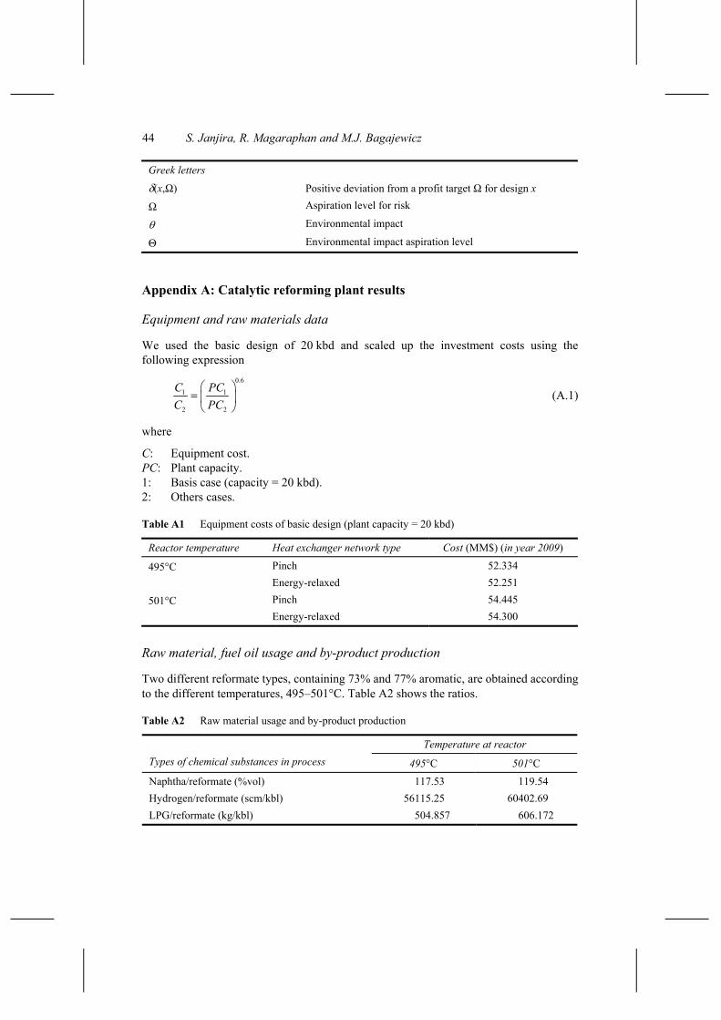
Greek letters

δ(x,Ω) Positive deviation from a profit target Ω for design x

Ω Aspiration level for risk

θ Environmental impact

Θ Environmental impact aspiration level

Appendix A: Catalytic reforming plant results

Equipment and raw materials data

We used the basic design of 20 kbd and scaled up the investment costs using the following expression

0.6

1 1

2 2

C PCC PC

=

(A.1)

where

C: Equipment cost. PC: Plant capacity. 1: Basis case (capacity = 20 kbd). 2: Others cases.

Table A1 Equipment costs of basic design (plant capacity = 20 kbd)

Reactor temperature Heat exchanger network type Cost (MM$) (in year 2009)

Pinch 52.334 495°C Energy-relaxed 52.251 Pinch 54.445 501°C Energy-relaxed 54.300

Raw material, fuel oil usage and by-product production

Two different reformate types, containing 73% and 77% aromatic, are obtained according to the different temperatures, 495–501°C. Table A2 shows the ratios.

Table A2 Raw material usage and by-product production

Temperature at reactor Types of chemical substances in process 495°C 501°C

Naphtha/reformate (%vol) 117.53 119.54 Hydrogen/reformate (scm/kbl) 56115.25 60402.69 LPG/reformate (kg/kbl) 504.857 606.172


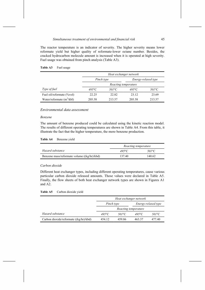
The reactor temperature is an indicator of severity. The higher severity means lower reformate yield but higher quality of reformate-lower octane number. Besides, the cracked hydrocarbon molecule amount is increased when it is operated at high severity. Fuel usage was obtained from pinch analysis (Table A3).

Table A3 Fuel usage

Heat exchanger network Pinch type Energy-relaxed type

Reacting temperature Type of fuel 495°C 501°C 495°C 501°C Fuel oil/reformate (%vol) 22.25 22.82 23.12 23.69 Water/reformate (m3/kbl) 205.58 213.57 205.58 213.57

Environmental data assessment

Benzene

The amount of benzene produced could be calculated using the kinetic reaction model. The results of different operating temperatures are shown in Table A4. From this table, it illustrate the fact that the higher temperature, the more benzene production.

Table A4 Benzene yield

Reacting temperature Hazard substance 495°C 501°C Benzene mass/reformate volume ((kg/hr)/kbd) 137.40 140.62

Carbon dioxide

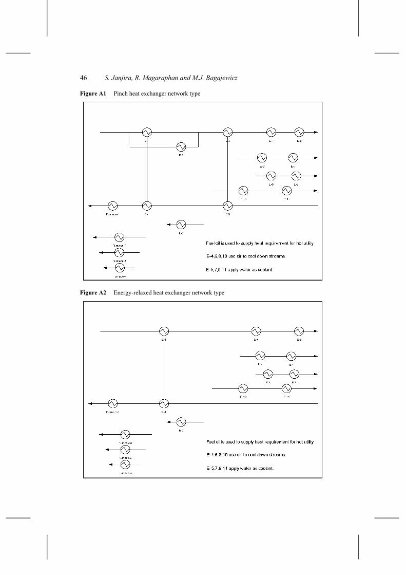
Different heat exchanger types, including different operating temperatures, cause various particular carbon dioxide released amounts. Those values were declared in Table A5. Finally, the flow sheets of both heat exchanger network types are shown in Figures A1 and A2.

Table A5 Carbon dioxide yield

Heat exchanger network Pinch type Energy-relaxed type

Reacting temperature Hazard substance 495°C 501°C 495°C 501°C Carbon dioxide/reformate ((kg/hr)/kbd) 454.12 459.86 463.37 477.40


Figure A1 Pinch heat exchanger network type

Figure A2 Energy-relaxed heat exchanger network type

Documents

Saran Janjira and Rathanawan Magaraphan* · Saran Janjira and Rathanawan Magaraphan* The Petroleum and Petrochemical College, Chulalongkorn University, ... was taken from the 1997