Embed Size (px)
Citation preview

AUTOMATIC CFD ANALYSIS METHOD FOR SHAPE OPTIMIZATION
Santiago Giraldo Arias
EAFIT UNIVERSITY
ENGINEERING SCHOOL
MECHANICAL ENGINEERING DEPARTMENT
MEDELLIN
2007
AUTOMATIC CFD ANALYSIS METHOD FOR SHAPE OPTIMIZATION
Graduation project for the degree of Mechanical Engineer
Advisor
Prof. Dr. Manuel Julio Garcia
EAFIT UNIVERSITY
ENGINEERING SCHOOL
MECHANICAL ENGINEERING DEPARTMENT
MEDELLIN
2007
Nota de Aceptacion
President of the Jury
Jury
Jury
Medellın, Nov 21 Of 2007

ACKNOWLEDGEMENTS
To my family, Luis Alberto, Luz Aida and Ana Catalina; all their faith and support has
brought me here. I hope tha I can repay you someday for the sacrifices you made
for me. All that I am or will become came from you and to you it will return.
I have come across many people during my carreer and the development of this
project. They have all contributed in their own manner to shape me as a better
person and engineer. The list falls short, this can only mean that a lot of people
have affected positively in my life. In particular I would like to thank my advisor,
Prof. Dr. Manuel J. Garcia, his support and guidance changed my perspective on
science and engineering, he also nurtured the desire to pursue my goals. Prof. Dr.
Pierre Boulanger, for his guidance, and opinions about science, engineering and
life encouraged my work on this field. Eng. Juan Duque, his solid work helped me
tremendously in the development of this project, yet his company and personality
made the workload feel lighter. To all the staff of the AMMI Lab and the Applied
Mechanics Lab, we have come a long way in such short time. This can only be a
sample of the great things to come, keep science fun.
To all my friends, wherever they are, again the list falls incredibly short, then I feel
blessed in many ways for this...
ABSTRACT
This project presents an Automatic Computational Fluid Dynamics (CFD) analysis
method for shape optimization of an aerodynamic profile. It begins with an overview
of basic concepts on shape optimization, geometry parameterization and objective
functions. It continues with an introduction to the current status of CFD simulation
software and types of solvers. Then expands to optimization based on CFD analysis.
Following, a CFD-based method to optimize aerodynamic profiles under certain re-
strictions and scenarios is proposed. Finally, the code implemented to automatically
modify a profile bound by a set of control points based on CFD analysis is described.
The project was developed entirely at the EAFIT University’s Applied Mechanics Lab-
oratory in Medellin, Colombia and is part of a collaboration effort in companionship
with the University of Aberta in Canada and Los Andes University in Bogota, Colom-
bia.
TABLE OF CONTENTS
0 STATE OF THE ART 9
0.1 SHAPE OPTIMIZATION 9
0.1.1 What is Shape Optimization. 9
0.1.2 Shape parameterization. 10
0.1.3 Objective Functions. 15
0.1.4 Optimization Methods. 17
0.2 AN INTRODUCTION TO COMPUTATIONAL FLUID DYNAMICS (CFD). 19
0.2.1 What is CFD. 19
0.2.2 CFD state of the art and current limitants. 22
0.2.3 CFD from the inside, an overview. 23
0.2.4 Discretization Schemes. 25
0.2.5 CFD flow behavior models. 27
0.3 AN INTRODUCTION TO WING AERODYNAMICS 28
0.3.1 Aerodynamic Variables. 29
0.3.2 Aerodynamic Forces and Moments. 30
0.3.3 Wing Profiles. 30
0.4 OPTIMIZATION IN COMPUTATIONAL FLUID DYNAMICS 33
1 METHODOLOGY 40
2 FOIL SHAPE OPTIMIZATION APPLICATION DESCRIPTION 46
2.1 Presentation. 46
2.2 Triangle 46
2.3 B-Curves 47
2.4 Netgen. 47
2.5 Data flow review. 49
2.6 Current application compilation. 50
2.7 Current foilOptimization application code Hints. 50
2.7.1 OpenFOAM patch detection over unstructured CFD doamin mesh. 51
2.7.2 Boundary condition setting over unstructured CFD domain mesh. 52
3 TESTS AND RESULTS 53
3.1 Overall review of reuslts 53
3.2 Optimization of NACA airfoils 54
3.3 Conceptual Examples 56
4 CONCLUSIONS AND FUTURE WORK 58
4.1 Conclusions. 58
4.2 Future Work. 59

BIBLIOGRAPHY 66

List of Tables
1 Relation between Mach number and flow regime 30
3.1 Comparisson between coefficients 53
List of Figures
1 CFD-Based optimization result of a turbine runner. 10
2 RAE2822 airfoil, degree-16 Bezier curvefit and control polygons asso-
ciated with the upper and lower surfaces. 12
3 PARSEC Method Parameters. 14
4 Sobieczky Method Parameters. 15
5 Three numerically derived orthogonal basis functions. 17
6 Steepest descent on a given space (local-global minima) 19
7 CFD Results (Displaying streamlines). 20
8 CFD Analysis for a injection valve system(Displaying streamlines). 21
9 Mount St. Helen’s Topography. 23
10 Mount St. Helen’s CFD domain over the Topography. 24
11 Aeroelasticity analysis by FEM. 26
12 Wing airfoil aerodynamic forces decomposition. 31
13 Wing airfoil typical regions. 31
14 Engine Cylce Modeling Sysem Components and Input/Outputs 35
15 CFD-Based Optimization, pressure distribution. Right: Original Wing,
Left: Optimized 36
16 CFD-Based Design System 37
17 Optimized guide vane and stay vane profiles 38
18 Original(Left) and Optimized (Right) ARA M-100 wing-body configu-
ration. Pressure distribution on the upper surface of the wing at M =
0.80, CL = 0.50. 39
1 Black Box Representation of the Method 42
2 Function decomposition 42
3 Build Airfoil Function Decomposition 43
4 Build Wing Function Decomposition 43
5 CFD module Decomposition 44
6 Geometry Manipulation Function Decomposition 44
7 Shape Optimization Function Decomposition 45
1 Required portions of the Netgen code (Highlighted) 48
2 Location and distribution of the source code of Netgen, BCurves, tri-
angle and foilOptimization. 49
1 Shape optimization of an example arbitrary profile 54
2 Case structure of an optimization 54
3 NACA0030 optimization 55
4 NACA0030 optimization CFD visualization 55
5 Representative airfoil optimization 56
6 CFD visualization of the airfoil raw case 57
0 STATE OF THE ART
The following chapter presents some relevant information to this study, from which
knowledge necessary for the development of the project can be obtained.
0.1 SHAPE OPTIMIZATION
0.1.1 What is Shape Optimization. Optimization in a broader sense is maximiz-
ing or minimizing some function relative to some set, often representing a range of
choices available in a certain situation. The function allows comparison of the dif-
ferent choices for determining which might fit better to the selection criteria (ROCK-
AFELLAR, 2007).
The maxima or minima of the function represent an important feature of the structure
(s). For example in a wing airfoil it can represent the minimum drag Coefficient Cd for
a given configuration. Then, if:
f(s) = min Cd (1)
The interest is to find the minimum of f(s), that is to find a s∗ such that:
f(s∗) = minf(s),∀ s ∈ V (2)
where V is the space of all the admissible geometries.
Shape optimization is within the field of optimal control theory. It is the process
of reaching an optimal shape through iteration over some design parameters. The
9
optimization process couples a geometry definition and analysis code in an itera-
tive process to produce optimum designs subject to various constraints (SONG y
KEANE, 2004). These constraints allow us to find a bounded set that defines the
optimal shape.
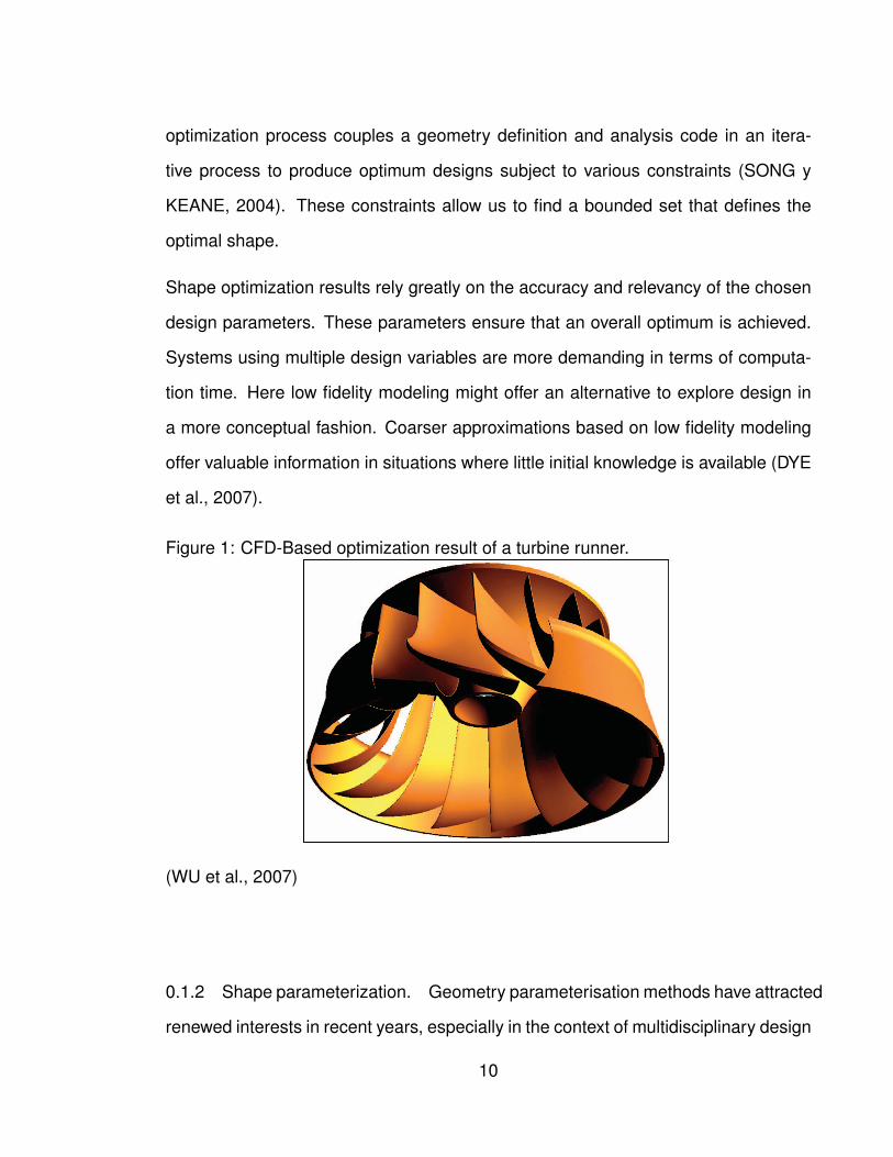
Shape optimization results rely greatly on the accuracy and relevancy of the chosen
design parameters. These parameters ensure that an overall optimum is achieved.
Systems using multiple design variables are more demanding in terms of computa-
tion time. Here low fidelity modeling might offer an alternative to explore design in
a more conceptual fashion. Coarser approximations based on low fidelity modeling
offer valuable information in situations where little initial knowledge is available (DYE
et al., 2007).
Figure 1: CFD-Based optimization result of a turbine runner.
(WU et al., 2007)
0.1.2 Shape parameterization. Geometry parameterisation methods have attracted
renewed interests in recent years, especially in the context of multidisciplinary design
10
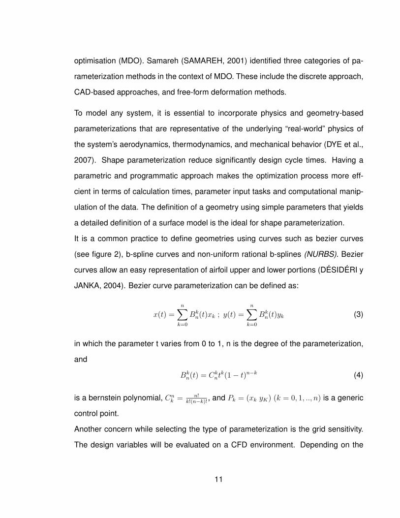
optimisation (MDO). Samareh (SAMAREH, 2001) identified three categories of pa-
rameterization methods in the context of MDO. These include the discrete approach,
CAD-based approaches, and free-form deformation methods.
To model any system, it is essential to incorporate physics and geometry-based
parameterizations that are representative of the underlying “real-world” physics of
the system’s aerodynamics, thermodynamics, and mechanical behavior (DYE et al.,
2007). Shape parameterization reduce significantly design cycle times. Having a
parametric and programmatic approach makes the optimization process more eff-
cient in terms of calculation times, parameter input tasks and computational manip-
ulation of the data. The definition of a geometry using simple parameters that yields
a detailed definition of a surface model is the ideal for shape parameterization.
It is a common practice to define geometries using curves such as bezier curves
(see figure 2), b-spline curves and non-uniform rational b-splines (NURBS). Bezier
curves allow an easy representation of airfoil upper and lower portions (DESIDERI y
JANKA, 2004). Bezier curve parameterization can be defined as:
x(t) =n∑
k=0
Bkn(t)xk ; y(t) =
n∑k=0
Bkn(t)yk (3)
in which the parameter t varies from 0 to 1, n is the degree of the parameterization,
and
Bkn(t) = Ck
ntk(1− t)n−k (4)
is a bernstein polynomial, Cnk = n!
k!(n−k)!, and Pk = (xk yK) (k = 0, 1, .., n) is a generic
control point.
Another concern while selecting the type of parameterization is the grid sensitivity.
The design variables will be evaluated on a CFD environment. Depending on the
11
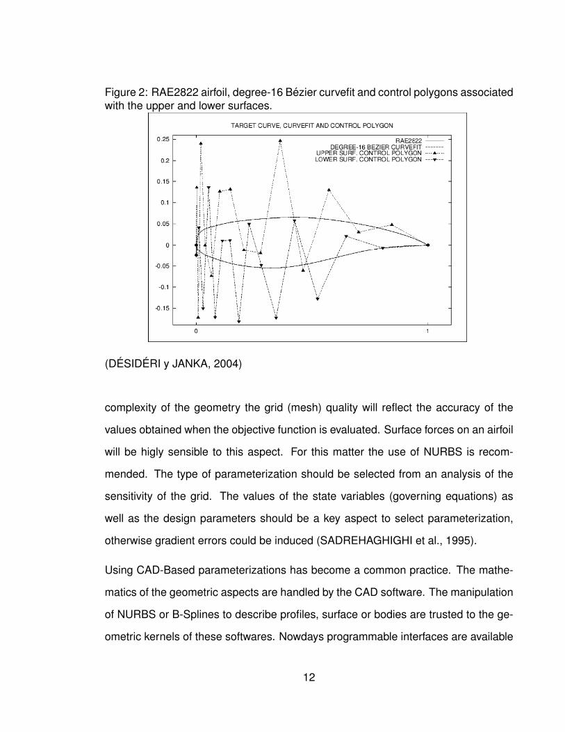
Figure 2: RAE2822 airfoil, degree-16 Bezier curvefit and control polygons associatedwith the upper and lower surfaces.
(DESIDERI y JANKA, 2004)
complexity of the geometry the grid (mesh) quality will reflect the accuracy of the
values obtained when the objective function is evaluated. Surface forces on an airfoil
will be higly sensible to this aspect. For this matter the use of NURBS is recom-
mended. The type of parameterization should be selected from an analysis of the
sensitivity of the grid. The values of the state variables (governing equations) as
well as the design parameters should be a key aspect to select parameterization,
otherwise gradient errors could be induced (SADREHAGHIGHI et al., 1995).
Using CAD-Based parameterizations has become a common practice. The mathe-
matics of the geometric aspects are handled by the CAD software. The manipulation
of NURBS or B-Splines to describe profiles, surface or bodies are trusted to the ge-
ometric kernels of these softwares. Nowdays programmable interfaces are available
12
for most of this softwares to enable code integration (DYE et al., 2007).
One of the key issues in deciding the parameterization method is to balance the
requirements of robustness and flexibility, and these decisions are also strongly de-
pendent on the goal of the design activity. Although some parameterization methods
may well be able to generate radical new shapes, this might not be suitable for de-
signs where the aim is to meet a specific pressure distribution or drag coefficient. In-
creased degrees of freedom in the control parameters -or elevated number of them-
will lead to a poor efficiency caused by the large search space that arises in the
optimization process (SONG y KEANE, 2004).
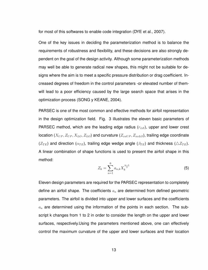
PARSEC is one of the most common and effective methods for airfoil representation
in the design optimization field. Fig. 3 illustrates the eleven basic parameters of
PARSEC method, which are the leading edge radius (rLE), upper and lower crest
location (XUP , ZUP , XLO, ZLO) and curvature (ZxxUP , ZxxLO), trailing edge coordinate
(ZTE) and direction (αTE), trailing edge wedge angle (βTE) and thickness (4ZTE).
A linear combination of shape functions is used to present the airfoil shape in this
method:
Zk =6∑
n=1
an,kXn−1
2k (5)
Eleven design parameters are required for the PARSEC representation to completely
define an airfoil shape. The coefficients an are determined from defined geometric
parameters. The airfoil is divided into upper and lower surfaces and the coefficients
an are determined using the information of the points in each section. The sub-
script k changes from 1 to 2 in order to consider the length on the upper and lower
surfaces, respectively.Using the parameters mentioned above, one can effectively
control the maximum curvature of the upper and lower surfaces and their location
13
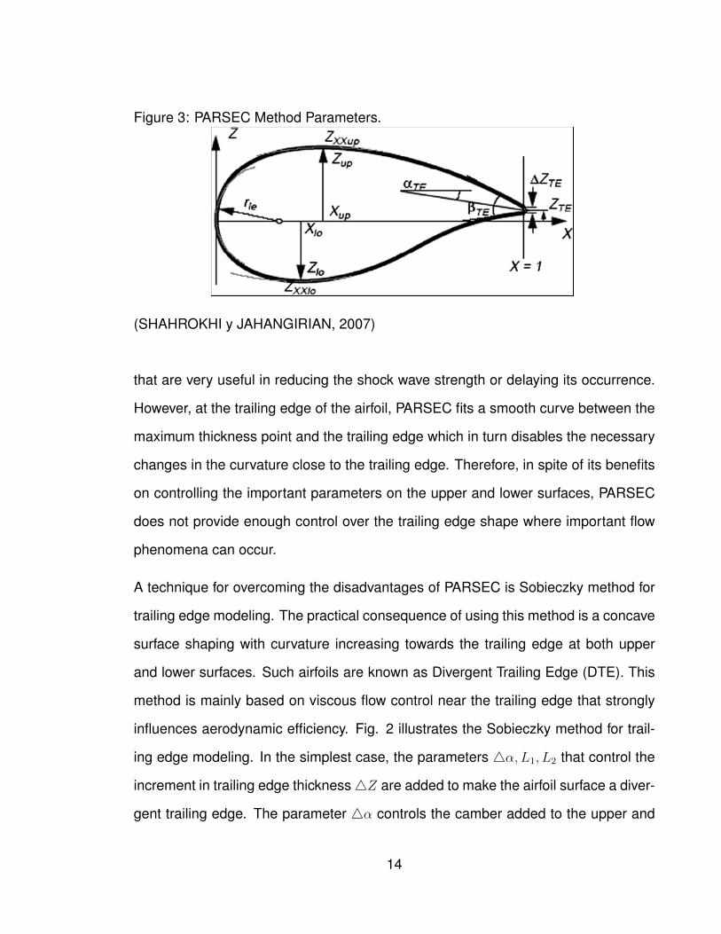
Figure 3: PARSEC Method Parameters.
(SHAHROKHI y JAHANGIRIAN, 2007)
that are very useful in reducing the shock wave strength or delaying its occurrence.
However, at the trailing edge of the airfoil, PARSEC fits a smooth curve between the
maximum thickness point and the trailing edge which in turn disables the necessary
changes in the curvature close to the trailing edge. Therefore, in spite of its benefits
on controlling the important parameters on the upper and lower surfaces, PARSEC
does not provide enough control over the trailing edge shape where important flow
phenomena can occur.
A technique for overcoming the disadvantages of PARSEC is Sobieczky method for
trailing edge modeling. The practical consequence of using this method is a concave
surface shaping with curvature increasing towards the trailing edge at both upper
and lower surfaces. Such airfoils are known as Divergent Trailing Edge (DTE). This
method is mainly based on viscous flow control near the trailing edge that strongly
influences aerodynamic efficiency. Fig. 2 illustrates the Sobieczky method for trail-
ing edge modeling. In the simplest case, the parameters 4α, L1, L2 that control the
increment in trailing edge thickness 4Z are added to make the airfoil surface a diver-
gent trailing edge. The parameter 4α controls the camber added to the upper and
14
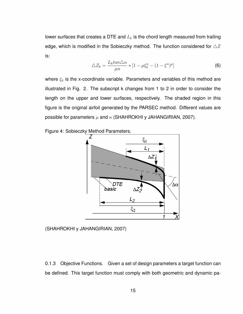
lower surfaces that creates a DTE and Lk is the chord length measured from trailing
edge, which is modified in the Sobieczky method. The function considered for 4Z
is:
4Zk =Lktan4α
µn∗ [1− µξn
k − (1− ξn)µ] (6)
where ξk is the x-coordinate variable. Parameters and variables of this method are
illustrated in Fig. 2. The subscript k changes from 1 to 2 in order to consider the
length on the upper and lower surfaces, respectively. The shaded region in this
figure is the original airfoil generated by the PARSEC method. Different values are
possible for parameters µ and n (SHAHROKHI y JAHANGIRIAN, 2007).
Figure 4: Sobieczky Method Parameters.
(SHAHROKHI y JAHANGIRIAN, 2007)
0.1.3 Objective Functions. Given a set of design parameters a target function can
be defined. This target function must comply with both geometric and dynamic pa-
15
rameters, hence the importance of the incorporation of accurate physics models. In
a CFD-based design process target functions must be evaluated several times until
design specifications are met (WU et al., 2007).
To define what an optimum design is after an optimization process, it is necessary
to establish the quality of the shape generated. An equation that represents all the
criteria defining the characterisitcs to improve in the design must be introduced. The
minimization of this expression (objective function) will lead to an optimum design
(FERRANO et al., 2004).
A possible definition of the objective function (OF) is an aggregation function with
weighted coefficients ck - see (Eq. 0.1.3)-, defining the relevance factors of each
single objective Fk. with K weighting coefficients ck, k=1,...,K (GIANNAKOGLOU,
2002).
Faggr =K∑
k=1
ck ∗ Fk(x) (7)
(GIANNAKOGLOU, 2002)
In an design optimization process multiple objective functions can be involved, the
complexity of the parameterization scales and different approaches must be used. In
aerodynamic design it is common to use basis functions that describe the expected
behavior of the geometry given specific conditions, then a single optimization func-
tion might fail to express the desired objective. Combining with shape parameteri-
zation an approach models the geometry as the linear combination of a basis airfoil
and a set of perturbation functions, defined either analytically or numerically,These
coefficients of the perturbation functions involved are then considered as the design
variables. A set of such orthogonal basis functions - see figure 5 - are the functions
16
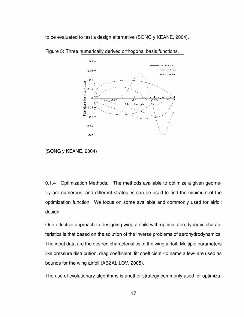
to be evaluated to test a design alternative (SONG y KEANE, 2004).
Figure 5: Three numerically derived orthogonal basis functions.
(SONG y KEANE, 2004)
0.1.4 Optimization Methods. The methods available to optimize a given geome-
try are numerous, and different strategies can be used to find the minimum of the
optimization function. We focus on some available and commonly used for airfoil
design.
One effective approach to designing wing airfoils with optimal aerodynamic charac-
teristics is that based on the solution of the inverse problems of aerohydrodynamics.
The input data are the desired characteristics of the wing airfoil. Multiple parameters
like pressure distribution, drag coefficient, lift coefficient -to name a few- are used as
bounds for the wing airfoil (ABZALILOV, 2005).
The use of evolutionary algorithms is another strategy commonly used for optimiza-
17
tion processes. Specifically, the use of Genetic Algorithms (GAs), which are semi-
stochastic semi-deterministic optimization methods that are conveniently presented
using the metaphor of natural evolution. The GAs are based on the evaluation of
a set of solutions, called population. The population is treated with genetic opera-
tors: selection, crossover and mutation. All these operations include randomness.
The main point is that the probability of survival of new individuals depends on their
fitness: the best are kept with a high probability, the worst are rapidly discarded
(EPSTEIN y PEIGIN, 2006).
The steepest descent method is an iterative procedure used to accomplish optimiza-
tion. Starting from some initial geometry the best direction to move from the local
point of view is the direction of the steepest descent. This direction corresponds to
the negative of the gradient. That is:
sn+1 = sn − β ∗ ∇(f(sn))
‖ ∇(f(sn)) ‖(8)
where β is a constant to be determined (in an optimum way) and the gradient at sn
of f(s) can be approximated by forward-difference:
∂f(s)
∂si
|sn =f(sn +4si)− f(sn)
4si
(9)
or with a second order central-difference approximation (HAFTKA y Gudal, 1992):
∂f(s)
∂si
|sn =f(sn +4si)− f(sn −4si)
2 ∗ 4si
(10)
This method assumes the existence of only one local minimum (unimodal functions).
Under the existence of several valleys the algorithm will converge to the closest local
18
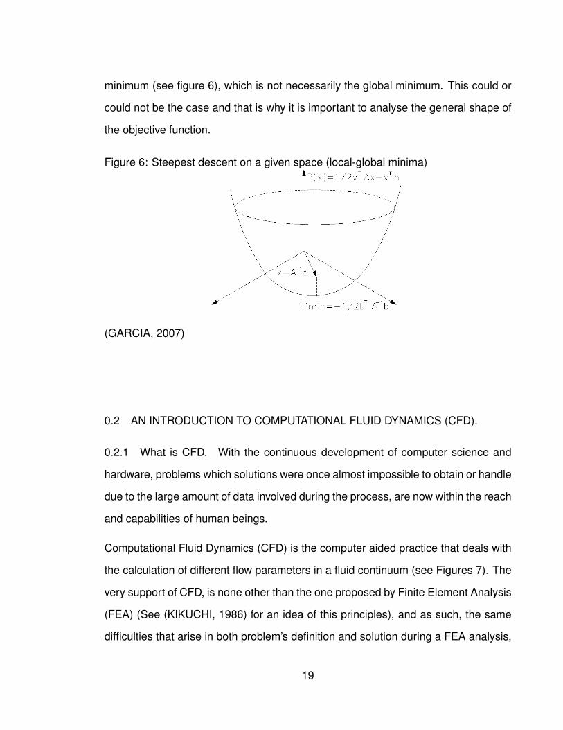
minimum (see figure 6), which is not necessarily the global minimum. This could or
could not be the case and that is why it is important to analyse the general shape of
the objective function.
Figure 6: Steepest descent on a given space (local-global minima)
(GARCIA, 2007)
0.2 AN INTRODUCTION TO COMPUTATIONAL FLUID DYNAMICS (CFD).
0.2.1 What is CFD. With the continuous development of computer science and
hardware, problems which solutions were once almost impossible to obtain or handle
due to the large amount of data involved during the process, are now within the reach
and capabilities of human beings.
Computational Fluid Dynamics (CFD) is the computer aided practice that deals with
the calculation of different flow parameters in a fluid continuum (see Figures 7). The
very support of CFD, is none other than the one proposed by Finite Element Analysis
(FEA) (See (KIKUCHI, 1986) for an idea of this principles), and as such, the same
difficulties that arise in both problem’s definition and solution during a FEA analysis,
19
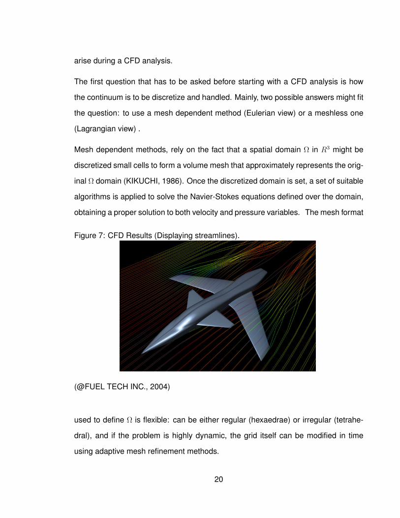
arise during a CFD analysis.
The first question that has to be asked before starting with a CFD analysis is how
the continuum is to be discretize and handled. Mainly, two possible answers might fit
the question: to use a mesh dependent method (Eulerian view) or a meshless one
(Lagrangian view) .
Mesh dependent methods, rely on the fact that a spatial domain Ω in R3 might be
discretized small cells to form a volume mesh that approximately represents the orig-
inal Ω domain (KIKUCHI, 1986). Once the discretized domain is set, a set of suitable
algorithms is applied to solve the Navier-Stokes equations defined over the domain,
obtaining a proper solution to both velocity and pressure variables. The mesh format
Figure 7: CFD Results (Displaying streamlines).
(@FUEL TECH INC., 2004)
used to define Ω is flexible: can be either regular (hexaedrae) or irregular (tetrahe-
dral), and if the problem is highly dynamic, the grid itself can be modified in time
using adaptive mesh refinement methods.
20
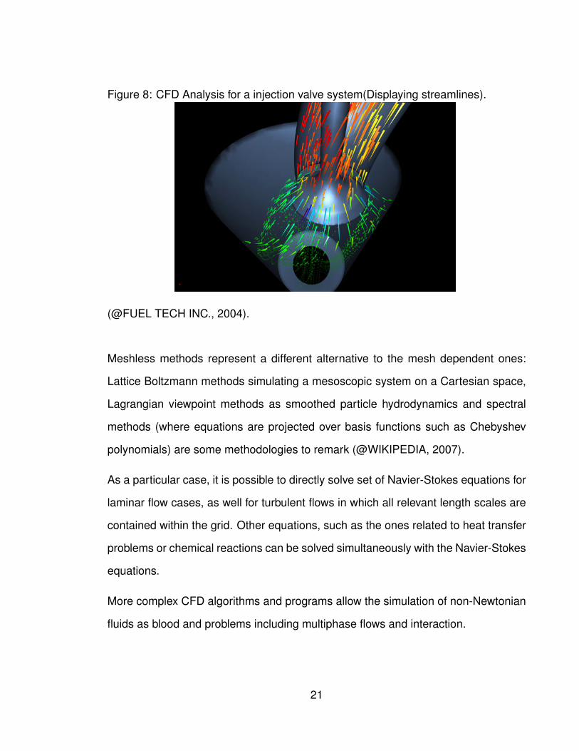
Figure 8: CFD Analysis for a injection valve system(Displaying streamlines).
(@FUEL TECH INC., 2004).
Meshless methods represent a different alternative to the mesh dependent ones:
Lattice Boltzmann methods simulating a mesoscopic system on a Cartesian space,
Lagrangian viewpoint methods as smoothed particle hydrodynamics and spectral
methods (where equations are projected over basis functions such as Chebyshev
polynomials) are some methodologies to remark (@WIKIPEDIA, 2007).
As a particular case, it is possible to directly solve set of Navier-Stokes equations for
laminar flow cases, as well for turbulent flows in which all relevant length scales are
contained within the grid. Other equations, such as the ones related to heat transfer
problems or chemical reactions can be solved simultaneously with the Navier-Stokes
equations.
More complex CFD algorithms and programs allow the simulation of non-Newtonian
fluids as blood and problems including multiphase flows and interaction.
21
0.2.2 CFD state of the art and current limitants. CFD is undergoing a significant
expansion in terms of both number of courses offered at universities and the number
of researchers active in the field. There are a number of software packages available
that solve fluid flow problems; the market is not as quite as large as the one for
structural mechanics codes. The lag can be explained by the fact CFD problems are,
in general, more difficult to solve. However, CFD codes are slowly being accepted
as design tools by industrial users (FERZIGER y PERIC, 2002) .
There are several commercially software packages available, such as FLUENT (@FLU-
ENT INC., 2007), CFX (@ANSYS INC., 2006) and STAR (@ADAPCO INC., 2006),
and open source code packages under the GPL license such as OpenFOAM (@OPEN
FOAM ORG., 2007). These packages contained within their source codes routines
and algorithms to solve incompressible, compressible and multiphase flows, direct
numerical and large eddy simulation, combustion and heat transfers problems, but
many particular cases and general problems are still impossible to solve with those
softwares.
Open source packages as OpenFOAM, even though their learning curve is steep,
represent an excellent solution for the dedicated engineer who wishes develop solu-
tions for unsolved problems.
One of the problems faced by CFD developers and users is none other than the one
of computational resources. CFD requires high amount of free memory to store up
data related to both calculations and results, as well fast processing units are needed
to perform the required operations, that could easily ascend to millions per iteration.
Parallel processing computing has been the answer to this problematic and right
now, big computer clusters are used by the market leaders to suffice their needs.
22
0.2.3 CFD from the inside, an overview. The CFD method may be subdivided into
3 large steps which cover the whole problem definition and solution process:
i. Pre-processing.
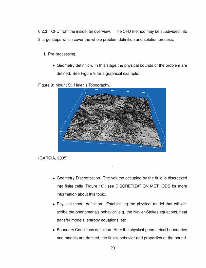
• Geometry definition. In this stage the physical bounds of the problem are
defined. See Figure 9 for a graphical example.
Figure 9: Mount St. Helen’s Topography.
(GARCIA, 2005)
.
• Geometry Discretization. The volume occupied by the fluid is discretized
into finite cells (Figure 10); see DISCRETIZATION METHODS for more
information about this topic.
• Physical model definition. Establishing the physical model that will de-
scribe the phenomena’s behavior; e.g. the Navier-Stokes equations, heat
transfer models, entropy equations, etc
• Boundary Conditions definition. After the physical-geometrical boundaries
and models are defined, the fluid’s behavior and properties at the bound-
23
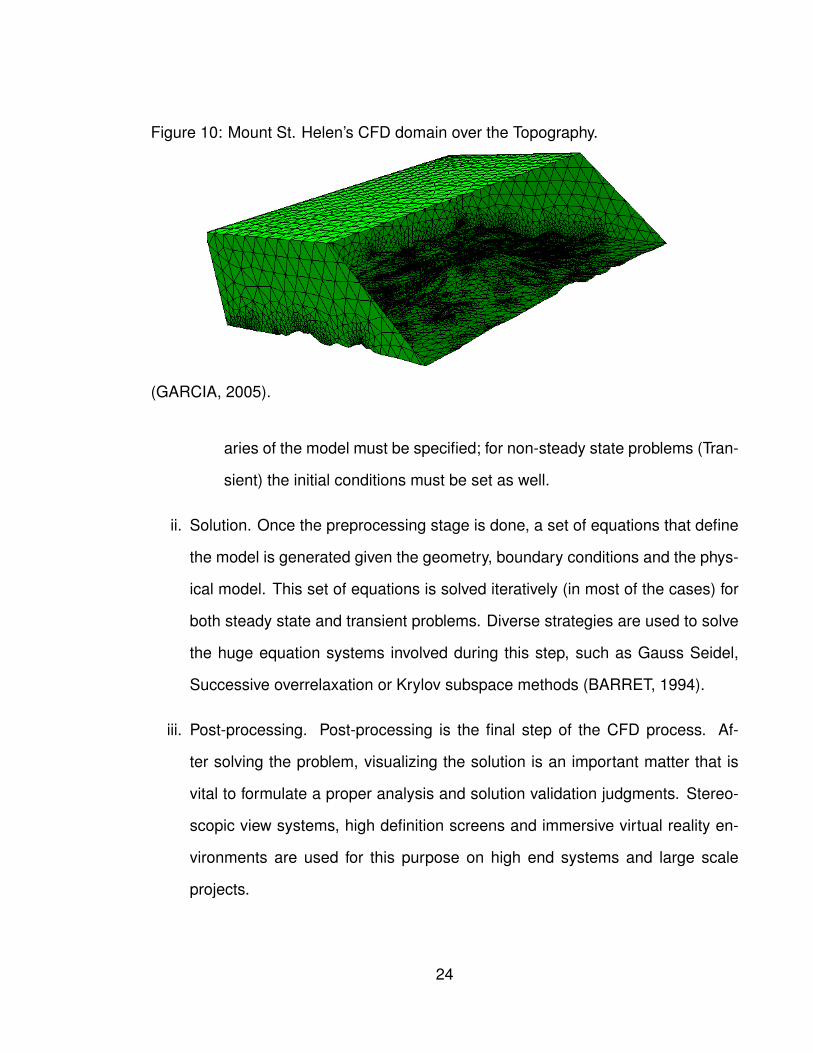
Figure 10: Mount St. Helen’s CFD domain over the Topography.
(GARCIA, 2005).
aries of the model must be specified; for non-steady state problems (Tran-
sient) the initial conditions must be set as well.
ii. Solution. Once the preprocessing stage is done, a set of equations that define
the model is generated given the geometry, boundary conditions and the phys-
ical model. This set of equations is solved iteratively (in most of the cases) for
both steady state and transient problems. Diverse strategies are used to solve
the huge equation systems involved during this step, such as Gauss Seidel,
Successive overrelaxation or Krylov subspace methods (BARRET, 1994).
iii. Post-processing. Post-processing is the final step of the CFD process. Af-
ter solving the problem, visualizing the solution is an important matter that is
vital to formulate a proper analysis and solution validation judgments. Stereo-
scopic view systems, high definition screens and immersive virtual reality en-
vironments are used for this purpose on high end systems and large scale
projects.
24
0.2.4 Discretization Schemes. The selection of a suitable discretization scheme
to solve a problem is one of the keys to success. For several problems, more than
one discretization scheme is appropriate and right on this spot is where the criterion
of the person who’s facing the situation is definitive (solution times might vary from
scheme to scheme exponentially for a given problem). Numerical stability is one of
the main goals one must pursue, and in most of the cases the discretization scheme
chosen is the one that fits best this condition. Some of the most used discretization
methods being used are:
Finite Volumes Method. This method responds to the principle that the governing
equations for the domain can be solved on discrete control volumes that rep-
resent the original domain; The integral approach for this method can be seen
on the following equation:
∂
∂t
∫Q dV +
∫F dA = 0 (11)
Where Q is the vector of conserved variables, dV is a differential of Volume,
F is the vector of fluxes and dA is the boundary of each differential of volume.
It is evident that this method is inherently conservative. This is a very popular
methodology on both commercial and open source codes.
Finite difference method. This method has historical importance and is simple to
program. It is currently only used in few specialized codes. The main disad-
vantage is that it requires structured meshes, and coordinate transformations
for complicated geometries (@WIKIPEDIA, 2007).
Finite Elements Method. The development of this methodology can be tracked
back to the 1940’s. The main idea of this approach is the possibility to divide
25
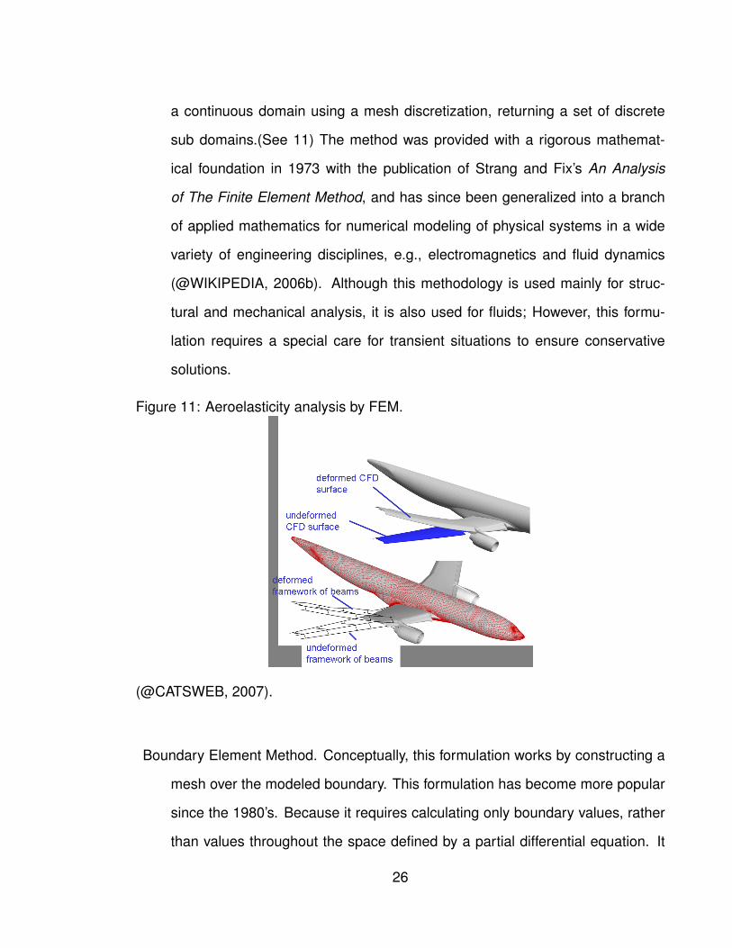
a continuous domain using a mesh discretization, returning a set of discrete
sub domains.(See 11) The method was provided with a rigorous mathemat-
ical foundation in 1973 with the publication of Strang and Fix’s An Analysis
of The Finite Element Method, and has since been generalized into a branch
of applied mathematics for numerical modeling of physical systems in a wide
variety of engineering disciplines, e.g., electromagnetics and fluid dynamics
(@WIKIPEDIA, 2006b). Although this methodology is used mainly for struc-
tural and mechanical analysis, it is also used for fluids; However, this formu-
lation requires a special care for transient situations to ensure conservative
solutions.
Figure 11: Aeroelasticity analysis by FEM.
(@CATSWEB, 2007).
Boundary Element Method. Conceptually, this formulation works by constructing a
mesh over the modeled boundary. This formulation has become more popular
since the 1980’s. Because it requires calculating only boundary values, rather
than values throughout the space defined by a partial differential equation. It
26
is significantly more efficient in terms of computational resources for problems
where there is a small surface/volume ratio (@WIKIPEDIA, 2006a).
0.2.5 CFD flow behavior models. Most flows encountered in engineering practice
are turbulent and therefore require different treatment. Turbulent flows are charac-
terized by the following properties (FERZIGER y PERIC, 2002):
• Turbulent flows are highly unsteady. A plot of the velocity as a function of time
at most points in the flow would appear random to an observer unfamiliar with
these flows. The word ’chaotic’ could be used but it has been given another
definition in recent years.
• They are three-dimensional. The time-averaged velocity may be a function of
only two coordinates, but the instantaneous field fluctuates rapidly in all three
spatial dimensions.
• They contain a great deal of vorticity. Indeed, vortex stretching is one of the
principal mechanisms by which the intensity of turbulence is increased.
• Turbulence increases the rate at which conserved quantities are stirred. Stirring
is a process in which parcels of fluid with differing concentrations of at least
one of the conserved properties are brought into contact. The actual mixing is
accomplished by diffusion. Nonetheless, this process is often called turbulent
diffusion.
• By means of the processes just mentioned, turbulence brings fluids of differing
momentum content into contact. The reduction of the velocity gradients due to
the action of viscosity reduces the kinetic energy of the flow; in other words,
27
mixing is a dissipative process. The lost energy is irreversibly converted into
internal energy of the fluid.
• It has been shown in recent years that turbulent flows contain coherent structures-
repeatable and essentially deterministic events that are responsible for a large
part of the mixing. However, the random component of turbulent flows causes
these events to differ from each other in size, strength, and time interval be-
tween occurrences, making study of them very difficult.
• Turbulent flows fluctuate on a broad range of length and time scales. This
property makes direct numerical simulation of turbulent flows very difficult.
0.3 AN INTRODUCTION TO WING AERODYNAMICS
Aerodynamics is an applied science dedicated to the study of the behavior of the air
when a body moves through it or a body opposes to its flow. One of the most impor-
tant manifestations of the interaction between fluid and solids is pressure. Pressure
is a measurable change of energy of the fluid molecules colliding with the surface
of the solid. For each point of the surface a pressure magnitude can be measured
(ANDERSON, 2001). In general efforts on the study of aerodynamics aim to:
• Prediction of forces and moments on, and heat transfer to, bodies moving
through a fluid. i.e. Lift, Drag, Moments, Heating of airfoil, airplanes, build-
ings, etc.
• Determination of flows moving through ducts. i.e. Calculation of air-breathing
jet engines, engine thrust, etc.
28
0.3.1 Aerodynamic Variables. The variables necessary to deal with an aerody-
namic study are described below (ANDERSON, 2001):
• Pressure is the normal force per unit area exerted on a surface due to the
change of momentum of gas molecules impacting the solid.
• Density is the mass per unit volume
• Temperature is the measure of kinetic energy of the molecules of the moving
fluid.
• Viscosity
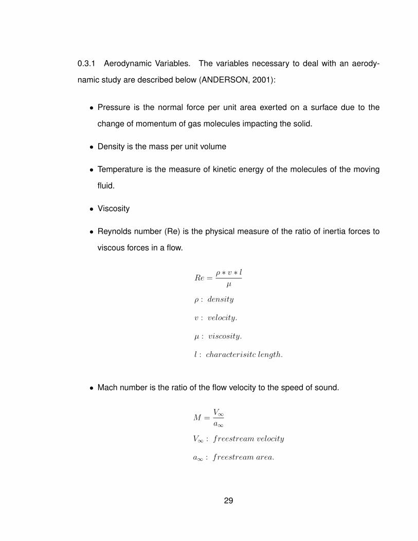
• Reynolds number (Re) is the physical measure of the ratio of inertia forces to
viscous forces in a flow.
Re =ρ ∗ v ∗ l
µ
ρ : density
v : velocity.
µ : viscosity.
l : characterisitc length.
• Mach number is the ratio of the flow velocity to the speed of sound.
M =V∞a∞
V∞ : freestream velocity
a∞ : freestream area.
29
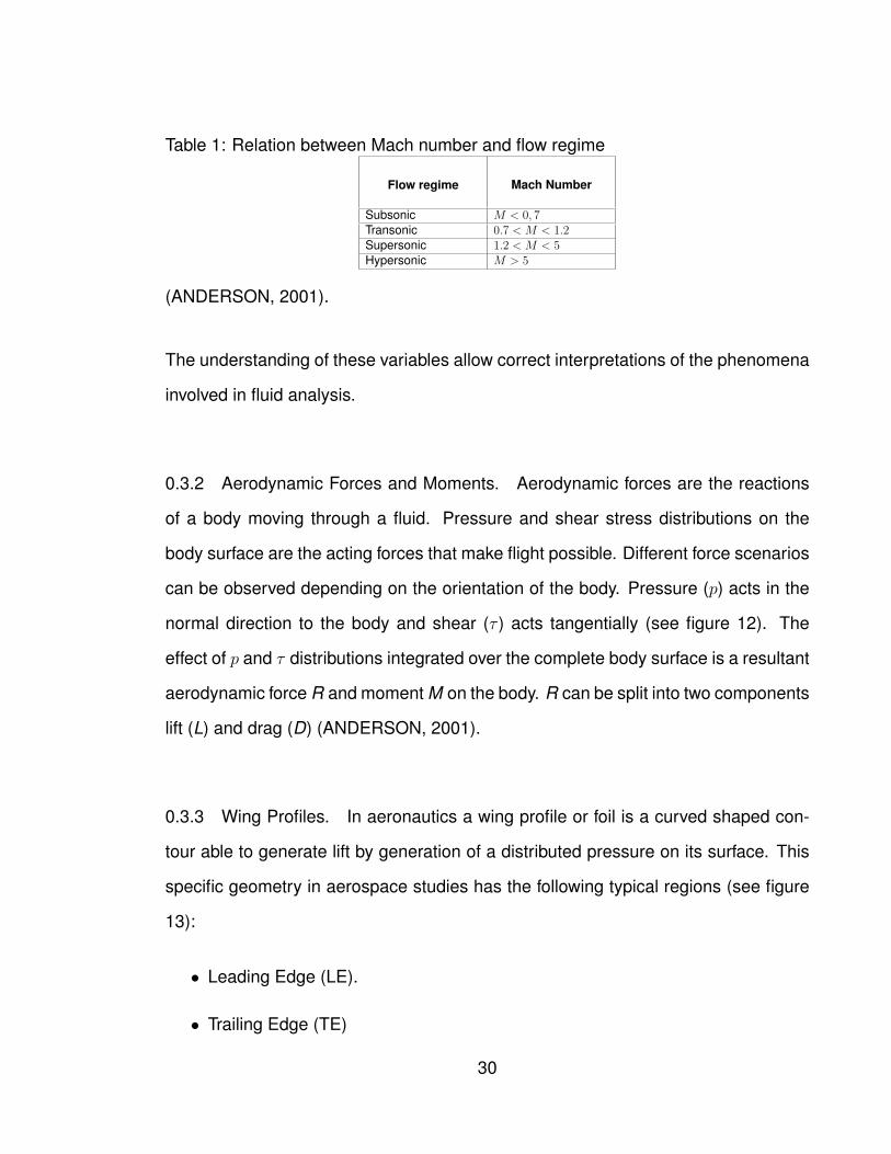
Table 1: Relation between Mach number and flow regime
Flow regime Mach Number
Subsonic M < 0, 7Transonic 0.7 < M < 1.2Supersonic 1.2 < M < 5Hypersonic M > 5
(ANDERSON, 2001).
The understanding of these variables allow correct interpretations of the phenomena
involved in fluid analysis.
0.3.2 Aerodynamic Forces and Moments. Aerodynamic forces are the reactions
of a body moving through a fluid. Pressure and shear stress distributions on the
body surface are the acting forces that make flight possible. Different force scenarios
can be observed depending on the orientation of the body. Pressure (p) acts in the
normal direction to the body and shear (τ ) acts tangentially (see figure 12). The
effect of p and τ distributions integrated over the complete body surface is a resultant
aerodynamic force R and moment M on the body. R can be split into two components
lift (L) and drag (D) (ANDERSON, 2001).
0.3.3 Wing Profiles. In aeronautics a wing profile or foil is a curved shaped con-
tour able to generate lift by generation of a distributed pressure on its surface. This
specific geometry in aerospace studies has the following typical regions (see figure
13):
• Leading Edge (LE).
• Trailing Edge (TE)
30
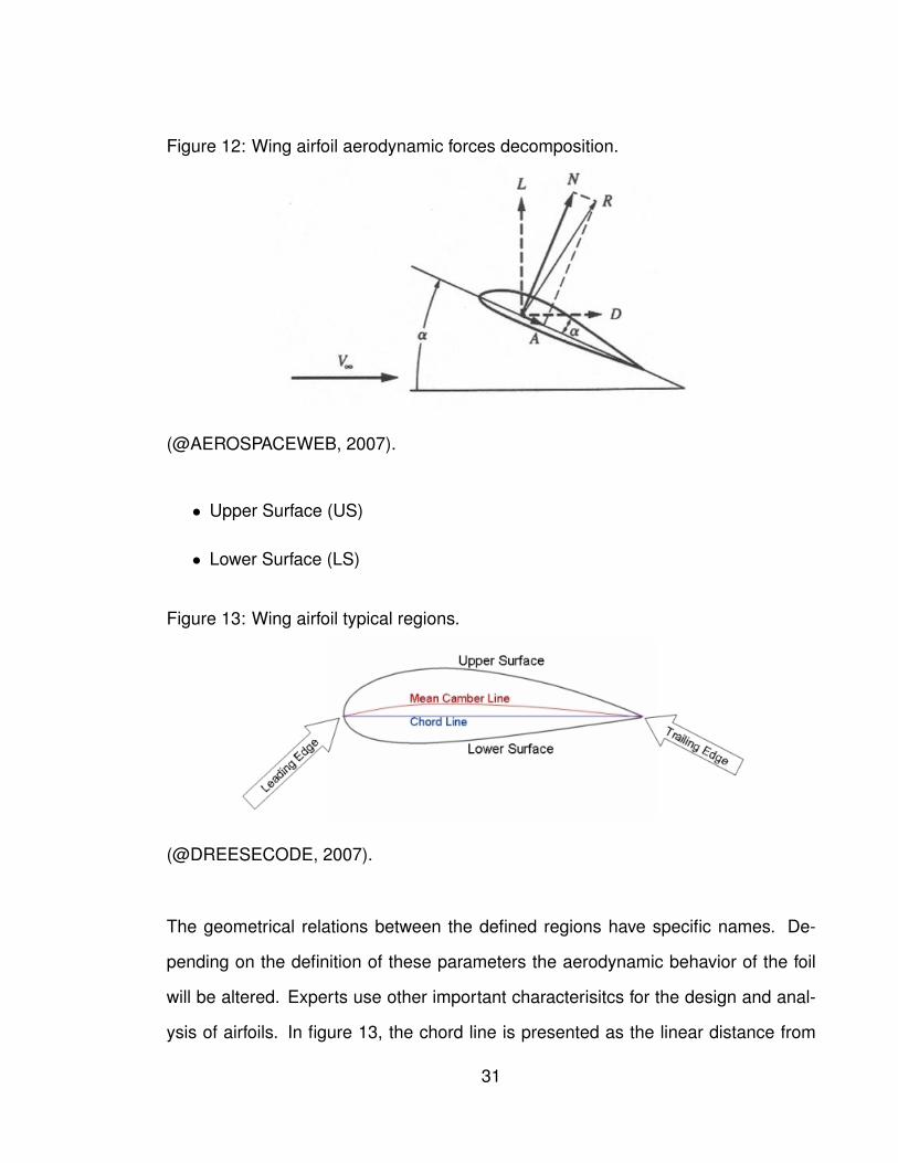
Figure 12: Wing airfoil aerodynamic forces decomposition.
(@AEROSPACEWEB, 2007).
• Upper Surface (US)
• Lower Surface (LS)
Figure 13: Wing airfoil typical regions.
(@DREESECODE, 2007).
The geometrical relations between the defined regions have specific names. De-
pending on the definition of these parameters the aerodynamic behavior of the foil
will be altered. Experts use other important characterisitcs for the design and anal-
ysis of airfoils. In figure 13, the chord line is presented as the linear distance from
31
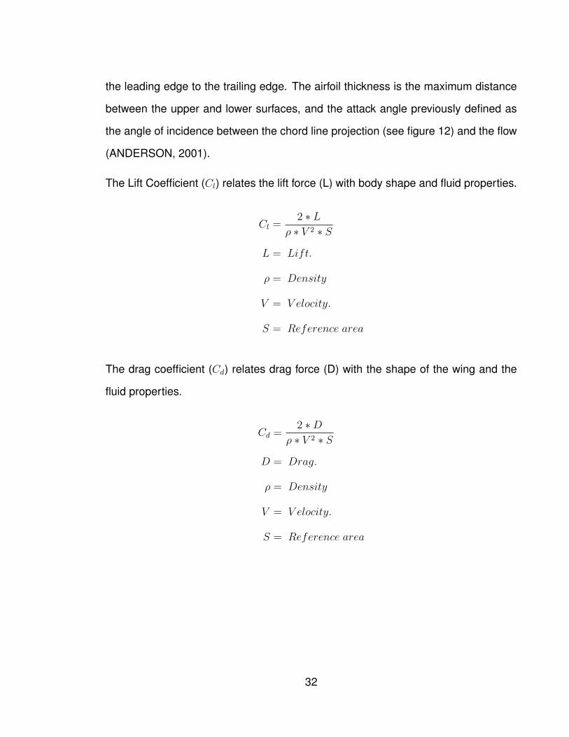
the leading edge to the trailing edge. The airfoil thickness is the maximum distance
between the upper and lower surfaces, and the attack angle previously defined as
the angle of incidence between the chord line projection (see figure 12) and the flow
(ANDERSON, 2001).
The Lift Coefficient (Cl) relates the lift force (L) with body shape and fluid properties.
Cl =2 ∗ L
ρ ∗ V 2 ∗ S
L = Lift.
ρ = Density
V = V elocity.
S = Reference area
The drag coefficient (Cd) relates drag force (D) with the shape of the wing and the
fluid properties.
Cd =2 ∗D
ρ ∗ V 2 ∗ S
D = Drag.
ρ = Density
V = V elocity.
S = Reference area
32
The moment coefficient (Cm) relates the twisting moment (M) to a point, usually this
point is set to 1/4 of the mean chord from the leading edge.
Cm =2 ∗M
ρ ∗ V 2 ∗ S
M = Moment.
ρ = Density
V = V elocity.
S = Reference area
The defined coefficients determine the correct behavior of wing profiles. An appropri-
ate combination of these variables for a given attack angle and speed yield smoother
results.
0.4 OPTIMIZATION IN COMPUTATIONAL FLUID DYNAMICS
CFD has come a long way since its beginings. The speed and capacity of the hard-
ware to manipulate huge sets of data has increased considerably. This capacity
allows to simulate complex fluid flow situations. Problems that were previously ad-
dressed with different disciplines are now approachable taking advantage of CFD.
The robustness offered by current CFD codes to solve the governing flow equations,
enable designers to obtain accurate preliminar field data to estimate the response of
new objects from virtual prototypes. One of the advantages of using CFD analysis
for optimization is to have multiple sets of data available at the same time (volumetric
fields). The possibility to analyze transient flow cases gives a head start to under-
stand the behavior of object in more realistic scenarios. Multiple efforts have been
33
carried out regarding coupling of CFD analysis and design optimization, several in-
house codes have been developed as well as existing cad tools and code integration.
As technological improvement and competition require more careful optimization
of designs or, when new high-technology applications demand prediction of flows
for which the database is insufficient, experimental development may be too costly
and/or timeconsuming. Optimization in these areas can produce large savings in
equipment and energy costs and in reduction of environmental pollution (FERZIGER
y PERIC, 2002).
The calculations obtained from CFD can be used for optimization regardless of the
complete accuray of the model. The predictions obtained when turbulence models
are used are not accurate enough that they can be accepted quantitatively without
testing. However, the trends may be accurately reproduced so that the design pre-
dicted to be the best by the model also performs the best in tests. Calculations
based on turbulence models can reduce the number of experimental tests required
and thus reduce the cost and the time required for development of a new product
(FERZIGER y PERIC, 2002).
The use of k-epsilon turbulence model is quite popular, although it has been known
that there is a deficiency in its performance for problems involving rotation and cur-
vature, the standard k-epsilon turbulence model is used in widely in studies for the
steady-state turbulent flow calculations,due to its robustness in practical applications
(WU et al., 2007).
Multidisclipinary Optimization (MDO) presents optimization on a new perspective.
34
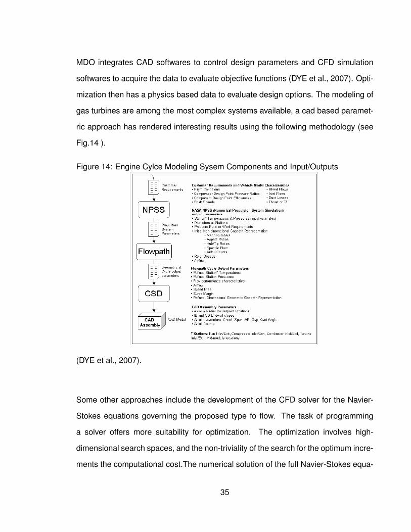
MDO integrates CAD softwares to control design parameters and CFD simulation
softwares to acquire the data to evaluate objective functions (DYE et al., 2007). Opti-
mization then has a physics based data to evaluate design options. The modeling of
gas turbines are among the most complex systems available, a cad based paramet-
ric approach has rendered interesting results using the following methodology (see
Fig.14 ).
Figure 14: Engine Cylce Modeling Sysem Components and Input/Outputs
(DYE et al., 2007).
Some other approaches include the development of the CFD solver for the Navier-
Stokes equations governing the proposed type fo flow. The task of programming
a solver offers more suitability for optimization. The optimization involves high-
dimensional search spaces, and the non-triviality of the search for the optimum incre-
ments the computational cost.The numerical solution of the full Navier-Stokes equa-
35
tions can be based on a multiblock code NES that employs structured point-to-point
matched grids.The key feature of NES is the use of the Essentially Non Oscilatory
(ENO) numerical scheme. The ENO approach is a high-order approximation scheme
designed for solutions containing discontinuities. In Navier-Stokes computations, the
scheme is usually applied to the approximation of convective terms (EPSTEIN y PEI-
GIN, 2006).
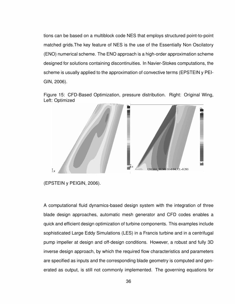
Figure 15: CFD-Based Optimization, pressure distribution. Right: Original Wing,Left: Optimized
(EPSTEIN y PEIGIN, 2006).
A computational fluid dynamics-based design system with the integration of three
blade design approaches, automatic mesh generator and CFD codes enables a
quick and efficient design optimization of turbine components. This examples include
sophisticated Large Eddy Simulations (LES) in a Francis turbine and in a centrifugal
pump impeller at design and off-design conditions. However, a robust and fully 3D
inverse design approach, by which the required flow characteristics and parameters
are specified as inputs and the corresponding blade geometry is computed and gen-
erated as output, is still not commonly implemented. The governing equations for
36
this phenomena are for turbulent flow, but the current assumptions still dwell on the
inviscid approach. A viscous CFD solver is needed. The design has to be evaluated
by the solver and the solution must be updated to modify the input (WU et al., 2007).
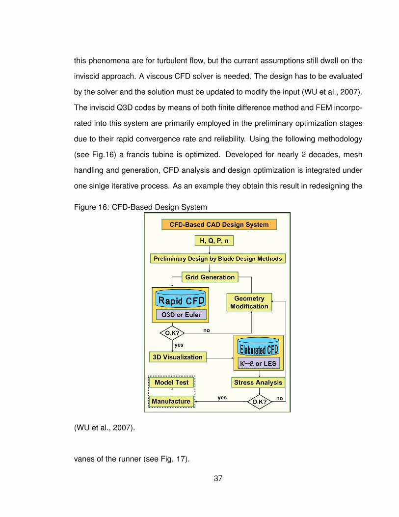
The inviscid Q3D codes by means of both finite difference method and FEM incorpo-
rated into this system are primarily employed in the preliminary optimization stages
due to their rapid convergence rate and reliability. Using the following methodology
(see Fig.16) a francis tubine is optimized. Developed for nearly 2 decades, mesh
handling and generation, CFD analysis and design optimization is integrated under
one sinlge iterative process. As an example they obtain this result in redesigning the
Figure 16: CFD-Based Design System
(WU et al., 2007).
vanes of the runner (see Fig. 17).
37
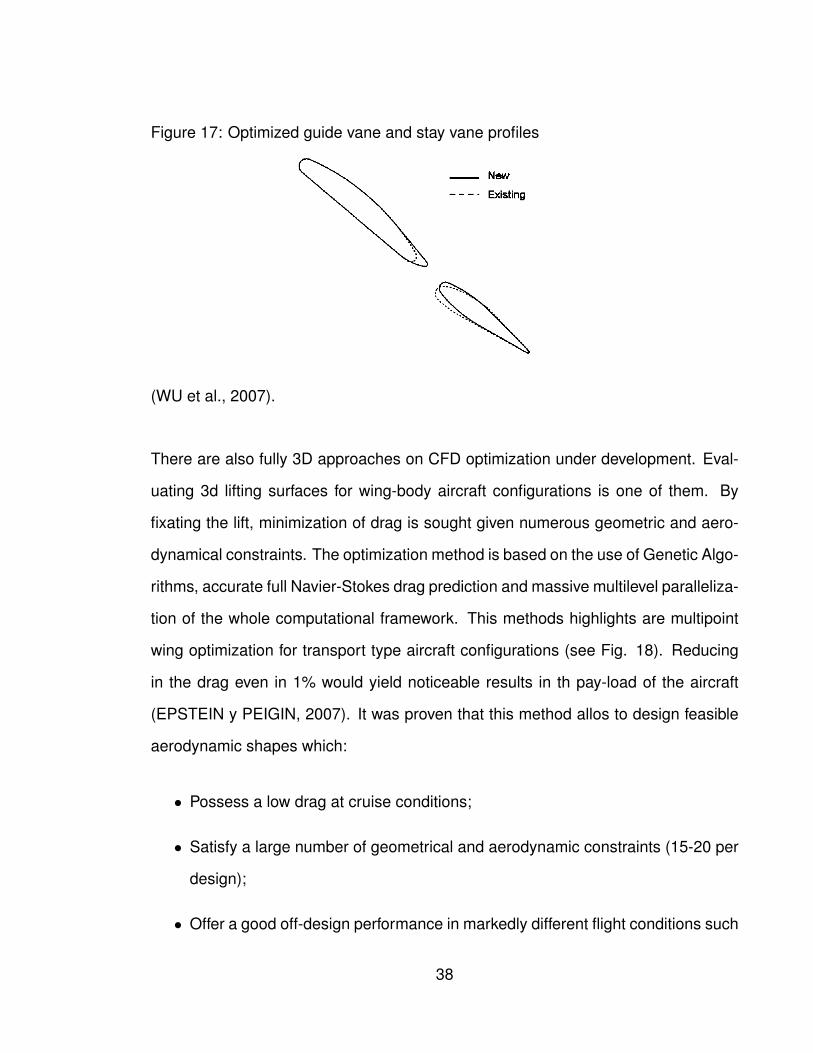
Figure 17: Optimized guide vane and stay vane profiles
(WU et al., 2007).
There are also fully 3D approaches on CFD optimization under development. Eval-
uating 3d lifting surfaces for wing-body aircraft configurations is one of them. By
fixating the lift, minimization of drag is sought given numerous geometric and aero-
dynamical constraints. The optimization method is based on the use of Genetic Algo-
rithms, accurate full Navier-Stokes drag prediction and massive multilevel paralleliza-
tion of the whole computational framework. This methods highlights are multipoint
wing optimization for transport type aircraft configurations (see Fig. 18). Reducing
in the drag even in 1% would yield noticeable results in th pay-load of the aircraft
(EPSTEIN y PEIGIN, 2007). It was proven that this method allos to design feasible
aerodynamic shapes which:
• Possess a low drag at cruise conditions;
• Satisfy a large number of geometrical and aerodynamic constraints (15-20 per
design);
• Offer a good off-design performance in markedly different flight conditions such
38
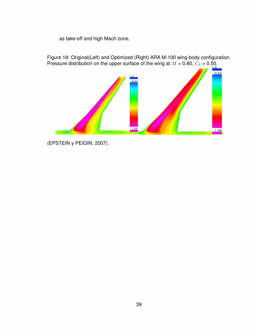
as take-off and high Mach zone.
Figure 18: Original(Left) and Optimized (Right) ARA M-100 wing-body configuration.Pressure distribution on the upper surface of the wing at M = 0.80, CL = 0.50.
(EPSTEIN y PEIGIN, 2007).
39
1 METHODOLOGY
The main objective is to produce a method that optimizes the shape of an aerody-
namic profile. To achieve this, we must define first the set of needs towards the
construction of the method itself. The process begins with the identification of the
disciplines to integrate:
i. Shape parameterization.
ii. Geometry manipulation.
iii. Aerodynamics.
iv. CFD-Based shape optimization.
v. Optimization methods (Gradient-based).
The steps to follow become the sewing thread between the mentioned disciplines.
They conform a road map of the whole process but it is not required to stay in se-
quential order. The basic scheme is presented as follows:
• Initially, a geometry is defined as the input and target of the method.
• The set of design variables are defined (they are a requirement of the method).
• Definition of the optimization functions.
• The geometry has to be represented as a data set that is portable between the
multiple tools.
• Parameterize the geometric characteristics of the body - to allow portability and
increase simplicity-.
40
• The geometry has to be prepared for CFD analysis, inlcuing generation of the
domain and boundary conditions.
• Adaptation of a chosen CFD solver to allow evaluation of optimization functions.
• Perform a CFD analysis on the given geometry, including embedded evaluation
of the optimization functions during run time.
• Manipulate the geometry based on the optimization method and criteria.
In general, if the process is contemplated as a black box it can be simplified to basic
input/output variables. The main I/O variables will begin the definition of the structure
of the method.
During any design process, feedback is an important step before any design alterna-
tive is chosen. The expertise of the designer can accelerate an optimization process
avoiding stagnation in local minima. This reason supports the need of offering a de-
gree of interaction between the optimization process and the user. Finding optimal
solutions with the minimal effort is foremost the objective to achieve, and reducing
the problems to its general form help to address their solution. Basically, the set of
tasks of the process can be reduced to the following needs:
• An application that integrates a set of tools to test and analyze automatically
an aerodynamic profile.
• A set of tools to perform the required tasks for the optimization process.
Then a black box representation like in Fig. 1 initiates the design process. Further
segregation proves itself useful in the definition of the tasks to perform. Placing the
problem in a form of structure before contemplating any data types (or specific so-
lution methods) can bring forth new sets of solutions. This strategy also reveals the
41
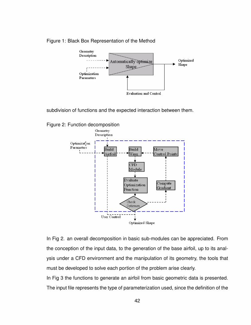
Figure 1: Black Box Representation of the Method
subdivision of functions and the expected interaction between them.
Figure 2: Function decomposition
In Fig 2. an overall decomposition in basic sub-modules can be appreciated. From
the conception of the input data, to the generation of the base airfoil, up to its anal-
ysis under a CFD environment and the manipulation of its geometry, the tools that
must be developed to solve each portion of the problem arise clearly.
In Fig 3 the functions to generate an airfoil from basic geometric data is presented.
The input file represents the type of parameterization used, since the definition of the
42
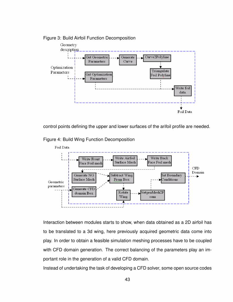
Figure 3: Build Airfoil Function Decomposition
control points defining the upper and lower surfaces of the arifoil profile are needed.
Figure 4: Build Wing Function Decomposition
Interaction between modules starts to show, when data obtained as a 2D airfoil has
to be translated to a 3d wing, here previously acquired geometric data come into
play. In order to obtain a feasible simulation meshing processes have to be coupled
with CFD domain generation. The correct balancing of the parameters play an im-
portant role in the generation of a valid CFD domain.
Instead of undertaking the task of developing a CFD solver, some open source codes
43
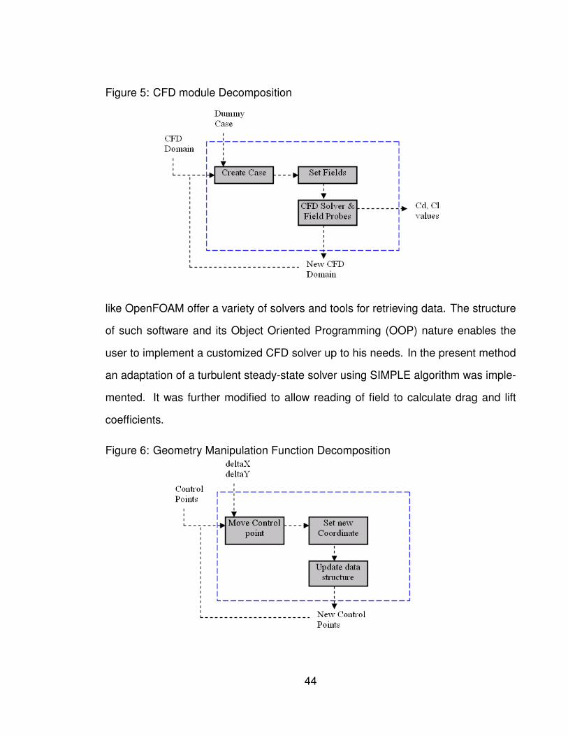
Figure 5: CFD module Decomposition
like OpenFOAM offer a variety of solvers and tools for retrieving data. The structure
of such software and its Object Oriented Programming (OOP) nature enables the
user to implement a customized CFD solver up to his needs. In the present method
an adaptation of a turbulent steady-state solver using SIMPLE algorithm was imple-
mented. It was further modified to allow reading of field to calculate drag and lift
coefficients.
Figure 6: Geometry Manipulation Function Decomposition
44
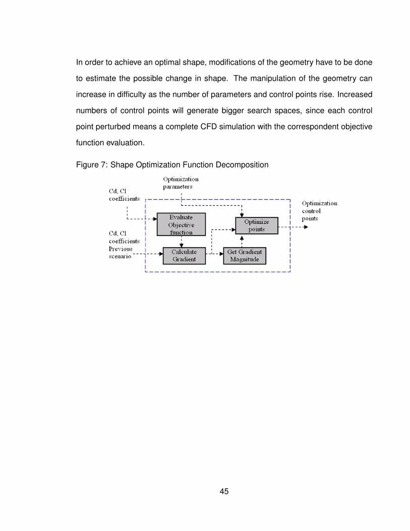
In order to achieve an optimal shape, modifications of the geometry have to be done
to estimate the possible change in shape. The manipulation of the geometry can
increase in difficulty as the number of parameters and control points rise. Increased
numbers of control points will generate bigger search spaces, since each control
point perturbed means a complete CFD simulation with the correspondent objective
function evaluation.
Figure 7: Shape Optimization Function Decomposition
45
2 FOIL SHAPE OPTIMIZATION APPLICATION DESCRIPTION
2.1 Presentation.
In this chapter, the user will find how to install the developed tool for airfoil shape opti-
mization, where the components are located and how to compile them. This chapter
consists of basic notes about Netgen (NG) installing and it’s requirements, triangle
code compilation, b-Curves library inclusion and OpenFOAM (OF) integration.
The foilOptimization application can be catalogued as an automatic CFD-based op-
timization solver for incompressible turbulente Navier-Stokes equations using the
SIMPLE algorithm. The original simpleFoam solver is adapted to allow drag and lift
readings during run time. This code is inehrently steady state, condition considered
to be accurate for the problem setup.
The foilOptimization application depends on a set of open source packages to per-
form the different operations required to manipulate the geometry, solve the CFD
problem and apply an optimization technique. In the following sections, each of the
applications will be briefly described at two levels: how to install it and how does it
interacts with the application.
2.2 Triangle
Inside the foilOptimization application, triangle is the tool that takes care of the 2D
triangulation of the polyline describing the airfoil. The data structures of triangle
are used throughout the code to preserve the definition of the geometry, and allow
regeneration of the airfoil polyline. For more information see SHEWCHUK (2007).
46
2.3 B-Curves
The role of B-Curves in the application is to provide the tools to manipulate B-Spline
curves for the parameterization of the profile geometry. B-Curves is a library pro-
grammed within the frame of the Applied Mechanics lab, it provides the underlying
structures for the manipulation of teh geometry. In combination with triangle they
represent a CAD emulation.
2.4 Netgen.
Inside the foilOptimization application, NG is the one who deals with the proper ac-
quisition of the wing’s boundary representation (B-REP) and in a later stage, the
generation of a valid triangular surface mesh to be used as the inner object repre-
sentation inside the CFD scenario.
The object’s B-REP is acquired from a combination of the integration of the triangle
code and own-developed tools to generate a 3d wing from a 2d profile. Currently,
valid ASCII Stereolitography (STL) are used for geometry acquisition, providing valid
engineering tolerances for design process.
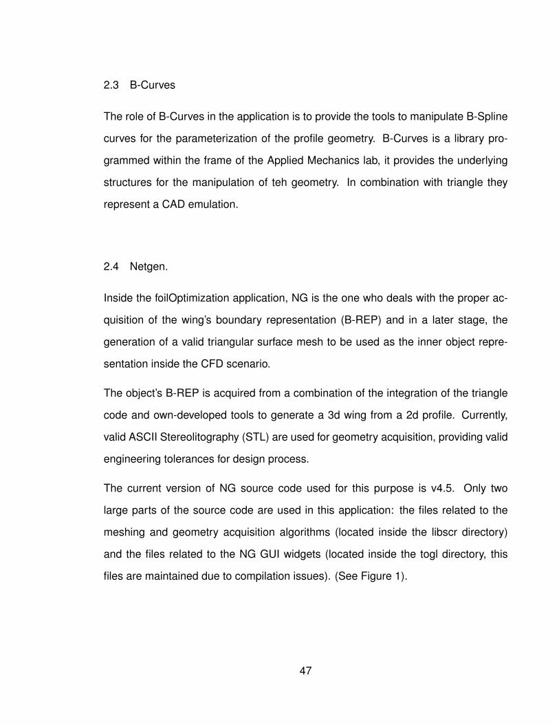
The current version of NG source code used for this purpose is v4.5. Only two
large parts of the source code are used in this application: the files related to the
meshing and geometry acquisition algorithms (located inside the libscr directory)
and the files related to the NG GUI widgets (located inside the togl directory, this
files are maintained due to compilation issues). (See Figure 1).
47
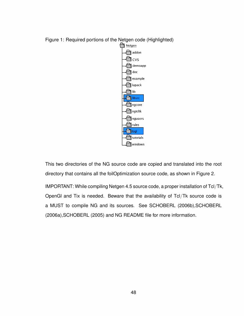
Figure 1: Required portions of the Netgen code (Highlighted)
This two directories of the NG source code are copied and translated into the root
directory that contains all the foilOptimization source code, as shown in Figure 2.
IMPORTANT: While compiling Netgen 4.5 source code, a proper installation of Tcl/Tk,
OpenGl and Tix is needed. Beware that the availability of Tcl/Tk source code is
a MUST to compile NG and its sources. See SCHOBERL (2006b),SCHOBERL
(2006a),SCHOBERL (2005) and NG README file for more information.
48
Figure 2: Location and distribution of the source code of Netgen, BCurves, triangle
and foilOptimization.
2.5 Data flow review.
Given a geometry and design variables defined by an user, this application optimizes
the shape of an airfoil. The input data file allows some degree of interactivity since it
allows to stop the process at any stage. The selection of the parameters sometimes
must be done intuitively. The input file is the option of interaction between the code
and the user to iterate over this parameters.
The inputs required are the control points, triangulation parameters, meshing pa-
rameters, optimization parameters, and 3d geometry data. The increased number
of inputs is a consequence of generalization of the application; for each geometry
(and depending on its complexity) different meshing and optimization parameters
are needed, otherwise, teh method will not converge.
49
2.6 Current application compilation.
The root directory of the fiolOptimization application source code is currently to be
located on the same directory where all the OF solvers for incompressible flow are
positioned (simpleFoam, boundaryFoam, nonNewtonianIcoFoam, etc...). This direc-
tory can be reached (after a proper OF installation and setting of system variables)
at $FOAM APP/solvers/incompressible.
The main directory is called foilOptimization, it contains a basic makefile (Makefile)
that compiles the application’s library (libfoilOptim) that contains all the NG, Bcurves,
Triangle and other objects of the foilOptimization application, to be linked later with
the other OF libraries using OpenFOAM’s own wmake. All the required files for
wmake compilation of the application are located at:
$FOAM APP/solvers/incompressible/foilOptimization/Make
. For more information about how does wmake works, see WMA (2000-2007).
To compile the application, just type in the command line (while being in the $FOAM APP/solvers/incompressible/foilOptimization
directory) make. The application’s executable will be placed on the same directory,
under the name foilOptimization.
2.7 Current foilOptimization application code Hints.
The foilOptimization source code lies mainly on 5 files, with the following description:
• foilOptimization.C: This file contains the main routine of the application and it’s
the starting point of it. Here all the pieces of code meet, a set of functions are
defined in this file regarding CFD solving and CFD domain generation.
50
• CFD DomainMesh.cpp: This file contains all the functions to manipulate the
CFD domain generated using netgen.
• CFD DomainMesh.H: Contains all the defines (Classes, constants and macros
required in the CFD DomainMesh.cpp file).
• Airfoil.cpp: Contains the methods to manipulate, construct and evaluate teh
geometry under the parameters of the optimization, it integrates BCurves.C
and Triangle.C to allow geometry generation and manipulation.
• Airfoil.h: It contains the defines, class methods, constants needed by Air-
foil.cpp.
2.7.1 OpenFOAM patch detection over unstructured CFD doamin mesh. During
the construction of a fvMesh, the user must supply to OF a valid list of indexed
boundary faces. Having explicit information about those boundary faces (Do they
belong to the boundary with the object? or, Do they belong to the CFD Domain
boundary?).
After performing the generation of the fvMesh given the cell data (vertex, cell types
and connectivity), OF catalogues all the un-neighbored faces of each cell by default
as defaultFaces, and storages each face index into a list. As a post-condition, all
the boundary faces of the CFD doamin are stored into a single list, which only has
information about indexes.
Extracting the boundary of the CFD domain is still insufficient to perform the CFD
analysis: It is still needed information about where to establish the boundary condi-
tions on the geometry. OF uses a figure, called patch to map the desired boundary
conditions over grouped set of faces.
51
2.7.2 Boundary condition setting over unstructured CFD domain mesh. After fil-
tering the OF patches, boundary conditions are to be set over them. The correspon-
dant boundary conditions, as defined by OF, should be as follows:
i. Object Boundary: Fixed Walls.
ii. Inlet: Inlet (Velocity has to be set -use a dummyCase-).
iii. Outlet: Outlet (Fixed Pressure value).
iv. CFD domain Walls: symmetryPlanes.
52
3 TESTS AND RESULTS
The algorithm was tested using 6 different geometries, 3 of them were NACA profiles.
The results observed in the NACA standard pfofiles are encouraging, even thoough
these profiles are already tested. The other 3 geometries are just proof of concept’s
examples, they help to expand the understanding of the job done by the algorithm.
It is to be expected form aerodynamic principles that a decrease in drag will carry on
a decrease in lift. The objective is to achieve a decrease of drag with the minimal lift
loss possible.
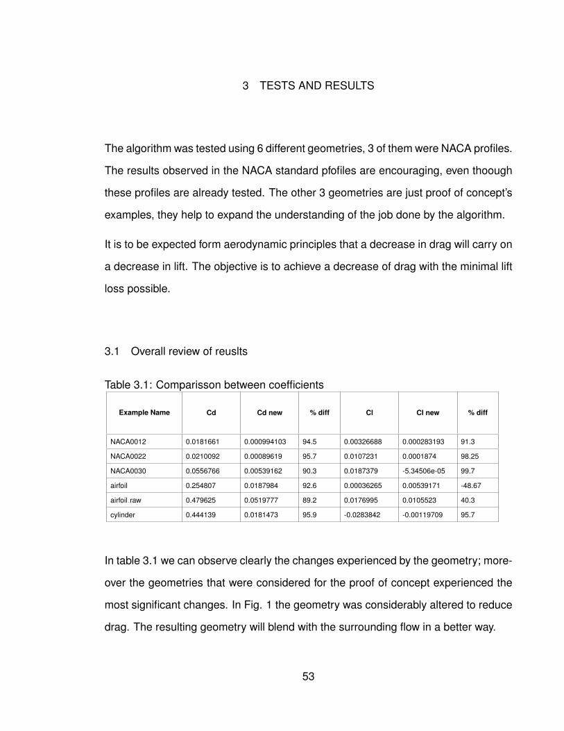
3.1 Overall review of reuslts
Table 3.1: Comparisson between coefficients
Example Name Cd Cd new % diff Cl Cl new % diff
NACA0012 0.0181661 0.000994103 94.5 0.00326688 0.000283193 91.3
NACA0022 0.0210092 0.00089619 95.7 0.0107231 0.0001874 98.25
NACA0030 0.0556766 0.00539162 90.3 0.0187379 -5.34506e-05 99.7
airfoil 0.254807 0.0187984 92.6 0.00036265 0.00539171 -48.67
airfoil raw 0.479625 0.0519777 89.2 0.0176995 0.0105523 40.3
cylinder 0.444139 0.0181473 95.9 -0.0283842 -0.00119709 95.7
In table 3.1 we can observe clearly the changes experienced by the geometry; more-
over the geometries that were considered for the proof of concept experienced the
most significant changes. In Fig. 1 the geometry was considerably altered to reduce
drag. The resulting geometry will blend with the surrounding flow in a better way.
53
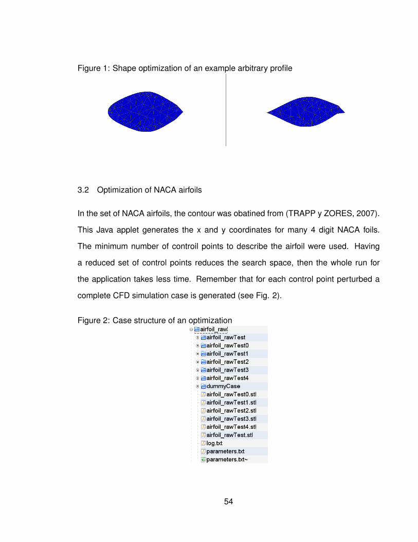
Figure 1: Shape optimization of an example arbitrary profile
3.2 Optimization of NACA airfoils
In the set of NACA airfoils, the contour was obatined from (TRAPP y ZORES, 2007).
This Java applet generates the x and y coordinates for many 4 digit NACA foils.
The minimum number of controil points to describe the airfoil were used. Having
a reduced set of control points reduces the search space, then the whole run for
the application takes less time. Remember that for each control point perturbed a
complete CFD simulation case is generated (see Fig. 2).
Figure 2: Case structure of an optimization
54
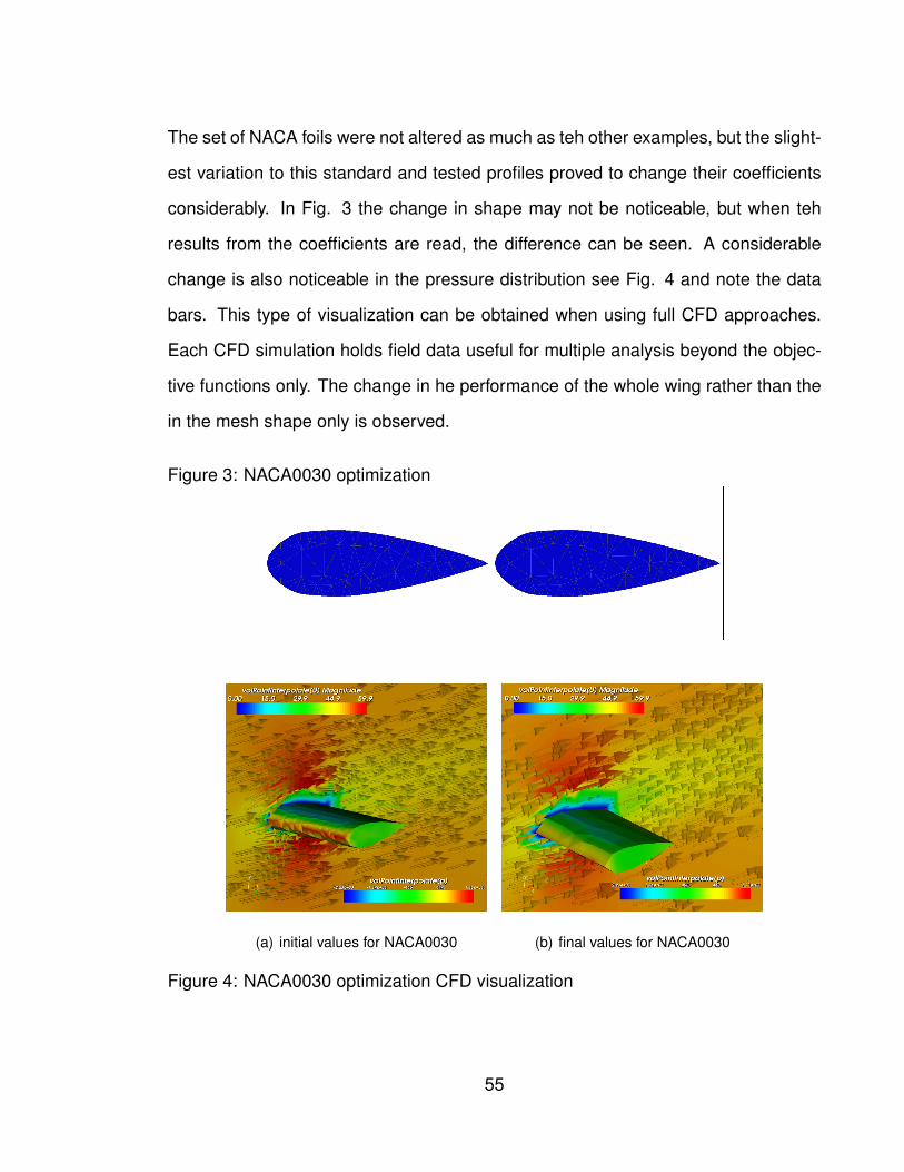
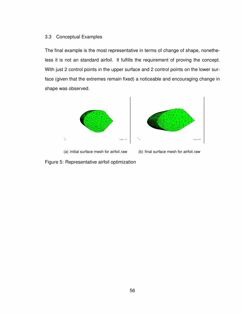
The set of NACA foils were not altered as much as teh other examples, but the slight-
est variation to this standard and tested profiles proved to change their coefficients
considerably. In Fig. 3 the change in shape may not be noticeable, but when teh
results from the coefficients are read, the difference can be seen. A considerable
change is also noticeable in the pressure distribution see Fig. 4 and note the data
bars. This type of visualization can be obtained when using full CFD approaches.
Each CFD simulation holds field data useful for multiple analysis beyond the objec-
tive functions only. The change in he performance of the whole wing rather than the
in the mesh shape only is observed.
Figure 3: NACA0030 optimization
(a) initial values for NACA0030 (b) final values for NACA0030
Figure 4: NACA0030 optimization CFD visualization
55
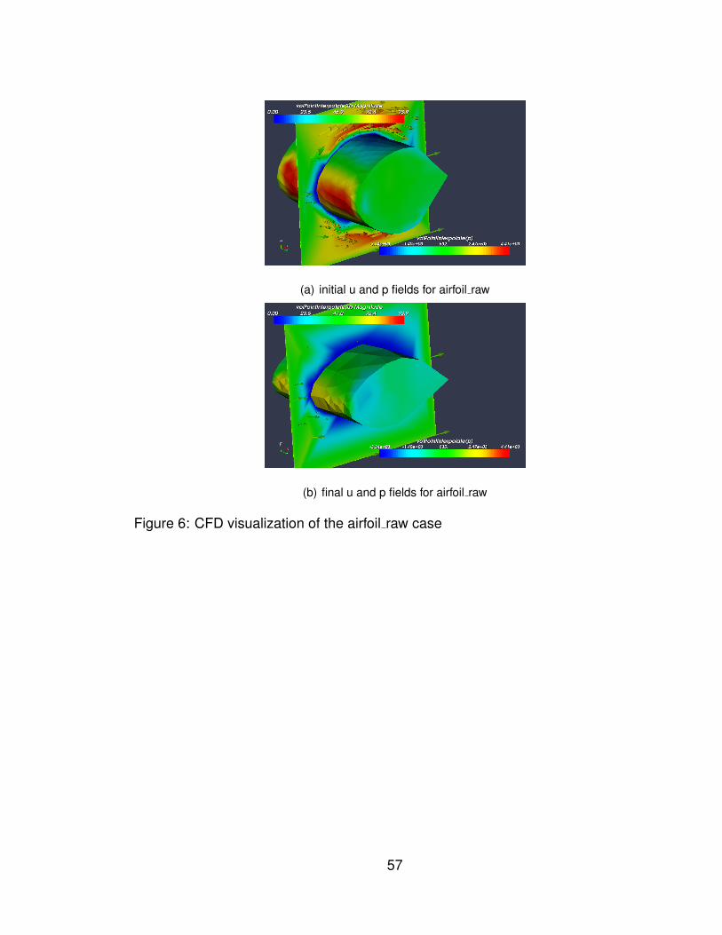
3.3 Conceptual Examples
The final example is the most representative in terms of change of shape, nonethe-
less it is not an standard airfoil. It fulfills the requirement of proving the concept.
With just 2 control points in the upper surface and 2 control points on the lower sur-
face (given that the extremes remain fixed) a noticeable and encouraging change in
shape was observed.
(a) initial surface mesh for airfoil raw (b) final surface mesh for airfoil raw
Figure 5: Representative airfoil optimization
56
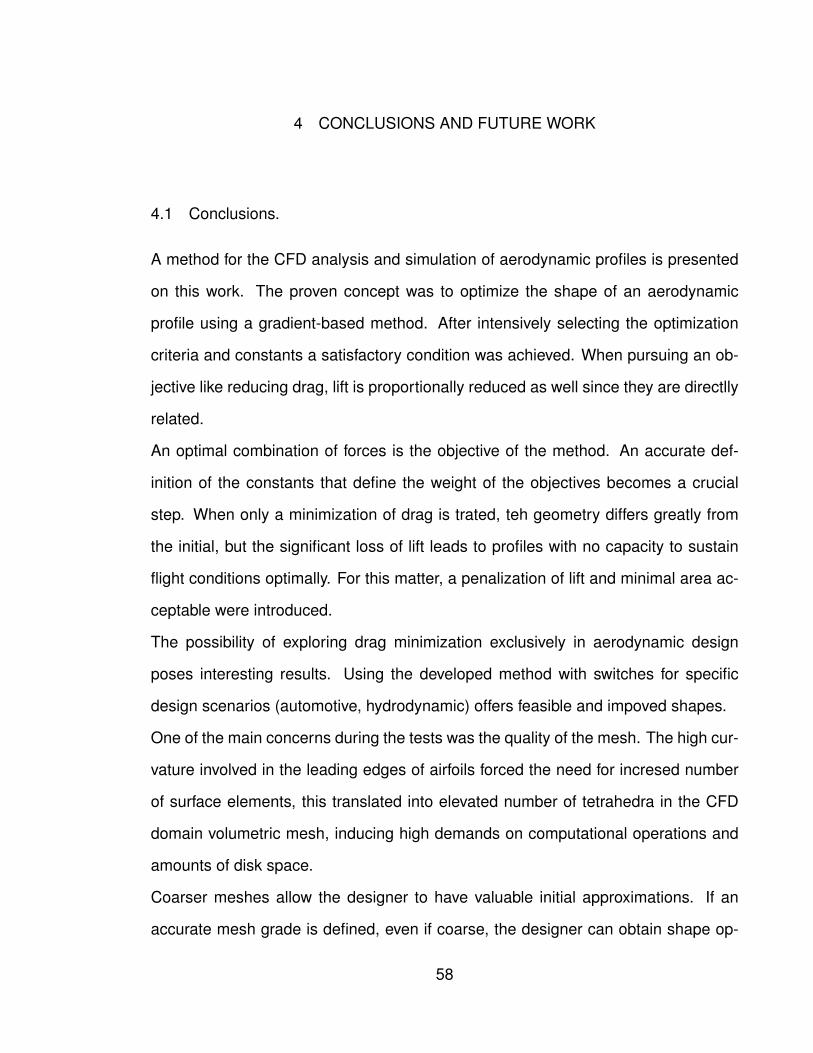
(a) initial u and p fields for airfoil raw
(b) final u and p fields for airfoil raw
Figure 6: CFD visualization of the airfoil raw case
57
4 CONCLUSIONS AND FUTURE WORK
4.1 Conclusions.
A method for the CFD analysis and simulation of aerodynamic profiles is presented
on this work. The proven concept was to optimize the shape of an aerodynamic
profile using a gradient-based method. After intensively selecting the optimization
criteria and constants a satisfactory condition was achieved. When pursuing an ob-
jective like reducing drag, lift is proportionally reduced as well since they are directlly
related.
An optimal combination of forces is the objective of the method. An accurate def-
inition of the constants that define the weight of the objectives becomes a crucial
step. When only a minimization of drag is trated, teh geometry differs greatly from
the initial, but the significant loss of lift leads to profiles with no capacity to sustain
flight conditions optimally. For this matter, a penalization of lift and minimal area ac-
ceptable were introduced.
The possibility of exploring drag minimization exclusively in aerodynamic design
poses interesting results. Using the developed method with switches for specific
design scenarios (automotive, hydrodynamic) offers feasible and impoved shapes.
One of the main concerns during the tests was the quality of the mesh. The high cur-
vature involved in the leading edges of airfoils forced the need for incresed number
of surface elements, this translated into elevated number of tetrahedra in the CFD
domain volumetric mesh, inducing high demands on computational operations and
amounts of disk space.
Coarser meshes allow the designer to have valuable initial approximations. If an
accurate mesh grade is defined, even if coarse, the designer can obtain shape op-
58
timization within minutes. The ability of the code to define a shape with few control
points presents and important advantage when the optimization process occurs. The
dimension of the search plays a vital role when defining the evolution of the shape,
having fewer control points reduces the size of the search space, enabling the de-
signer to obtain intial approximations faster.
A limitant when analyzing different shapes becomes the particular boundary condi-
tions of each shape for its CFD analysis, an interactive process to select this condi-
tions would prove itself useful. Setting the conditions of the turbulent solver are higly
case-dependent as well. In this work the k-epsilon model was used due to its robust-
ness in practical application. When high Reynolds numbers lead to the assumption
of a steady state flow condition, the k-epsilon model is used widely.
The process of constructing the shape in 3d from 2d control points and later on the
CFD domain became a time consuming task. A parametrical definition of the geom-
etry was implemented and allows the generation of various shapes with a valid CFD
domain. The CFD domain size is quite large when treating outside flows (like the
ones when simulating an arifoil moving through air) and causes simulation times to
increase considerably.
4.2 Future Work.
After proving the concept of CFD-based shape optimization in a single CPU, the code
will undergo changes to allow parallelization. Parallelization will allow more complex
geometries, more refined domains and shorter simulation times.
The current meshing process has to be reviewed for efficient adaptation to CFD
optimal conditions, possible use of more specific airfoil hexahedra mesh generation
will be explored using OpenFOAM’s embedded mesher “blockMesh“.
59
Exploring the integration with a CAD platform under Linux (the native environment
of the application) in C/C++ programming language would scale the usability of this
application. Currently the API of ProEngineer offers an alternative to such challenge.
Further study in optimization objective functions is yet to be done. Work has but
begun....
60
BIBLIOGRAPHY
OpenFOAM 1.4 User Guide. OpenCFD Ltd, 2000-2007. 3.2 Compiling applications
and libraries, Available with OpenFOAM.
ABZALILOV, D. F. Minimization of the Wing Airfoil Drag Coefficient Using the Optimal
Control Method. En : Fluid Dynamics tomo 40, no 6, p. 985–991, 2005.
@ADAPCO INC., . STAR CFD software. Web, 2006. Available at: http://www.
cd-adapco.com/.
@AEROSPACEWEB, . Lift and Drag vs. axial force. Web, 2007. Available at: http:
//www.aerospaceweb.org/question/aerodynamics/q0194.shtml.
ANDERSON, John D. Fundamentals Of Aerodynamics 3 ed. Mc Graw-Hill, 2001.
@ANSYS INC., . ANSYS/CFX CFD software. Web, 2006. Available at: http:
//www-waterloo.ansys.com/.
BARRET, R. Templates for the Solution of Linear Systems: Building Blocks for Itera-
tive Methods 2 ed. SIAM, Philadelphia, PA, 1994.
BRYSON, Steve y LEVIT, Creon. The Virtual Wind Tunnel. tomo 4. 1992.
C., ZIENKIEWICZ O. y TAYLOR, R. L. Finite Element Method: Volume 3, Fluid
Dynamics 5 ed. tomo 3. Butterworth-Heinemann, 2000.
@CATSWEB, . Lift and Drag vs. axial force. Web, 2007. Available at: http://www.
cats.rwth-aachen.de/research/images/f-deformed-dlr-f6.png.
DESIDERI, Jean-Antoine y JANKA, Ales. Multilevel Shape Parameterization For
Aerodynamic Optimization - Application To Drag And Noise Reduction Of Tran-
61
sonic/Supersonic Business Jet. En : European Congress on Computational Meth-
ods in Applied Sciences and Engineering ECCOMAS, 2004.
@DREESECODE, . Typical Airfoil Regions. Web, 2007. Available at: http://www.
dreesecode.com/primer/p2 f003.jpg.
DYE, Christopher; STAUBACH, Joseph B.; EMMERSON, Diane y JENSEN, C. Greg.
Cad-Based Parametric Cross-Section for Gas Turbine Engine MDO Applications.
En : Computer Aided Design and Applications tomo 4, no 1-4, p. 509–518, 2007.
EPSTEIN, B. y PEIGIN, S. Optimization of 3D wings based on Navier-Stokes so-
lutions and genetic algorithms. En : International Journal of Computational Fluid
Dynamics tomo 20, no 2, p. 75–92, 2006.
————. Accurate CFD driven optimization of lifting surfaces for wing-body config-
uration. En : Computers and Fluids, 2007.
FERRANO, Lluis; KUENY, Jean-Louis; AVELLAN, Francois y PEDRETTI, Laurant,
Camille TOMAS. Surface Parameterization of a Francis Runner Turbine for Opti-
mum Design. En : 22nd IAHR Symposium on Hydraulic Machinery and Systems,
2004.
FERZIGER, J.H. y PERIC, M. Computational Methods for Fluid Dynamics 3 ed.
Springer, 2002.
@FLUENT INC., . Parallel Processing. Web, 2006. Available at: http://www.
fluent.com/software/fidap/parallel.htm.
————. Fluent CFD software. Web, 2007. Available at: http://www.fluent.com/
software.
62
@FUEL TECH INC., . ACUITIV Software post-processor for CFD. Web, 2004. Avail-
able at: http://www.acuitiv.com/.
GARCIA, Manuel. Fixed Grid Finite Element Analysis in Structural Design and Opti-
misation. Tesis Doctoral Department of Aeronautical Engineering, The University
of Sydney, 1999.
————. Virtual Wind Tunnel Talk. University of Alberta, 2005. Talk conducted to
professors and students at the University of Alberta.
GARCIA, Manuel J. Lecture Notes on Numerical Analysis, 2007.
GIANNAKOGLOU, K. C. Design of Optimal Aerodynamic Shapes using Stochastic
Optimization Methods and Computational Intelligence. En : Progress in Aerospace
Sciences tomo 38, p. 43–76, 2002.
HAFTKA, R. y Gudal, Z. Finite Element Method: Volume 3, Fluid Dynamics 3 ed.
Kluwer Academic Publishers, 1992.
JARAMILLO, Juan David; VIDAL, Antonio M. y CORREA, Francisco Jose. Meto-
dos directos para la solucion de sistemas de ecuaciones lineales simetricos, in-
definidos, edispersos y de gran dimension. Investigation Booklet, DOCUMENT
40-022006, 2006. Chapter 5, Parallel Computing.
JASWAL, Vijendra. CAVEvis: Distributed Real-Time Visualization of Time-Varing
Scalar and Vector Fields Using the CAVE Virtual Reality theater. IEEE Visualiza-
tion Conference, 1997. Proceedings of the 8th IEEE Visualization Conference,
Phoenix, AZ. 301–308.
KIKUCHI, Noboru. Finite Element Methods in Mechanics 1 ed. Cambridge University
Press, 1986.
63
@MACHINE DESIGN, Magazine y MEDIA, PENTON. A better mesher for
FEA. Web, 2005. Available at: http://www.machinedesign.com/ASP/
viewSelectedArticle.asp?strArticleId=58645&strSite=MDSite&catId=0.
@OPEN FOAM ORG., . Open Foam CFD toolkit. Web, 2007. Available at: www.
opencfd.co.uk/openfoam/.
ROCKAFELLAR, R. T. Fundamentals Of Optimization, 2007.
SADREHAGHIGHI, Ideen; SMITH, Robert E. y TIWARI, Surendra N. Grid Sensitivity
and Aerodynamic Optimization of Generic Airfoils. En : Journal of Aircraft tomo 32,
no 6, 1995.
SAMAREH, J. A. Survey of shape parameterization techniques for high-fidelity mul-
tidisciplinary shape optimisation. En : AIAA tomo 39, no 5, p. 877–884, 2001.
SCHOBERL, Joachim. NETGEN 4.5 User Guide. Available with Netgen Distribution,
2005.
————. NETGEN - automatic mesh generator. Web, 2006a. http://www.hpfem.
jku.at/netgen/.
————. NETGEN - troubleshooting. Web, 2006b. http://www.hpfem.jku.at/
netgen/.
SHAHROKHI, Ava y JAHANGIRIAN, Alireza. Airfoil shape parameterization for op-
timum Navier-Stokes design with genetic algorithm. En : Aerospace Science and
Technology p. 2, 2007.
SHAW, Christopher D.; HALL, James A.; EBERT, David S. y ROBERTS, D. Aaron.
Interactive lens visualization techniques. p. 155–160. IEEE Visualization Confer-
ence, 1999.
64
SHEWCHUK, Jonathan Richard. A Two-Dimensional Quality Mesh Generator and
Delaunay Triangulator. Web, 2007. http://www.cs.cmu.edu/∼quake/triangle.
html.
SONG, Wenbin y KEANE, Andrew J. A Study of Shape Parameterisation Methods
for Airfoil Optimisation. En : AIAA p. 1, 2004.
TRAPP, Jens y ZORES, Robert. Applet to generate NACA 4 digit airfoils. Web, 2007.
http://www.pagendarm.de/trapp/programming/java/profiles/NACA4.html.
VICINI, A. y QUAGLIARELLA, D. Airfoil and wing design through hybrid optimization
strategies. En : AIAA p. 27–29, 1998.
Wiki, OpenFOAM. simpleFoam. Web, 2007. http://gcdw05.unileoben.ac.at/
non cdl/OpenFOAMWiki/index.php/simpleFoam.
@WIKIPEDIA, . Computational fluid dynamics. Web, 2007. Available at: http:
//en.wikipedia.org/wiki/Computational fluid dynamics.
@WIKIPEDIA, The free encyclopedia. Boundary element method. Web, 2006a.
Available at: http://en.wikipedia.org/wiki/Boundary Element Method.
————. Finite element method. Web, 2006b. Available at: http://en.wikipedia.
org/wiki/FEM.
————. Parallel computing. Web, 2006c. Available at: http://en.wikipedia.
org/wiki/Parallel computing.
————. Real time programming. Web, 2006d. Available at: http://en.
wikipedia.org/wiki/Real-time.
65

WU, Jinchung; SHIMMEI, Katsumasa; TANI, Kiyohito; Joushirou, SATO y NIIKURA,
Kazuo. CFD-Based Design Optimization for HydroTurbines. En : Journal Of Fluids
Engineering tomo 129/159, 2007.
66