Embed Size (px)
Citation preview

SALES AND MARKUP DISPERSION:
THEORY AND EMPIRICS∗
Monika Mrazova†
University of Geneva,
and CEPR
J. Peter Neary‡
University of Oxford,
CEPR and CESifo
Mathieu Parenti§
ULB and CEPR
September 7, 2017
∗Earlier versions were circulated under the title “Technology, Demand, and the Size Distribution ofFirms”. We are particularly grateful to Jan De Loecker and Julien Martin for assisting us with the data,and to Abi Adams, Costas Arkolakis, Jonathan Dingel, Peter Egger, Basile Grassi, Joe Hirschberg, OlegItskhoki, Luca Macedoni, Rosa Matzkin, Marc Melitz, Steve Redding, Kevin Roberts, Ina Simonovska, StefanSperlich, Gonzague Vannoorenberghe, Frank Verboven, Frank Windmeijer, Tianhao Wu, and participants atvarious conferences and seminars for helpful comments. Monika Mrazova thanks the Fondation de FamilleSandoz for funding under the “Sandoz Family Foundation - Monique de Meuron” Programme for AcademicPromotion. Peter Neary thanks the European Research Council for funding under the European Union’sSeventh Framework Programme (FP7/2007-2013), ERC grant agreement no. 295669.†Geneva School of Economics and Management (GSEM), University of Geneva, Bd. du Pont d’Arve 40,
1211 Geneva 4, Switzerland; e-mail: [email protected].‡Department of Economics, University of Oxford, Manor Road, Oxford OX1 3UQ, UK; e-mail: pe-
[email protected].§ECARES, Universite Libre de Bruxelles, Av. F.D. Roosevelt, 42, 1050 Brussels, Belgium; mpar-

Abstract
We derive exact conditions relating the distributions of firm productivity, sales,
output, and markups to the form of demand. In particular, for a large family (including
Pareto, lognormal, and Frechet), the distributions of productivity and sales are the
same if and only if demand is “CREMR” (Constant Revenue Elasticity of Marginal
Revenue). Based on this demand function, we uncover a new class of distributions
that are well-suited to capture the dispersion of markups. Empirically, we show that
the choice between Pareto and lognormal productivity distributions matters less in
explaining sales and markups than the choice between CREMR and other demands.
Keywords: CREMR Demands; Heterogeneous Firms; Kullback-Leibler Divergence; Lognor-
mal Distribution; Pareto Distribution; Sales and Markup Distributions.
JEL Classification: F15, F23, F12

1 Introduction
The hypothesis of a representative agent has provided a useful starting point in many fields
of economics. However, sooner or later, intellectual curiosity and the exigencies of match-
ing the empirical evidence make it essential to recognize that agents are heterogeneous. In
many cases, this involves constructing models with three components. First is a distribution
of agent characteristics, usually assumed exogenous; second is a model of individual agent
behavior; and third, implied by the first two, is a predicted distribution of outcomes. Such
a pattern can be seen in income distribution theory, in the theory of optimal income taxa-
tion, in macroeconomics, and in urban economics.1 In the field of international trade it has
rapidly become the dominant paradigm, since the increasing availability of firm-level export
data from the mid-1990s onwards undermined the credibility of representative-firm models,
and stimulated new theoretical developments. A key contribution was Melitz (2003), who
built on Hopenhayn (1992) to derive an equilibrium model of monopolistic competition with
heterogeneous firms. In this setting, the model structure combines assumptions about the
distribution of firm productivity and about the form of demand that firms face to derive pre-
dictions about the distribution of firm sales. Such models have provided a fertile laboratory
for studying a wide range of problems relating to the process of globalization.
Although the pioneering work of Melitz (2003) avoided making specific distributional
assumptions, trade models have typically been parameterized in a canonical way, that com-
bines a Pareto distribution of firm productivity on the supply side with CES preferences on
the demand side. As shown by Helpman, Melitz, and Yeaple (2004) and Chaney (2008), this
combination of assumptions predicts a Pareto distribution of firm sales. This parametriza-
tion can be justified on at least two grounds. First is its theoretical tractability, which makes
it relatively easy to extend the model to incorporate various real-world features of the global
economy, such as outsourcing, multi-product firms, and global value chains.2 Second is the
1For examples, see Stiglitz (1969), Mirrlees (1971), Krusell and Smith (1998), and Behrens, Duranton,and Robert-Nicoud (2014), respectively.
2See Antras and Helpman (2004), Bernard, Redding, and Schott (2011), and Antras and Chor (2013),

empirical regularity that the distribution of firm sales is plausibly close to Pareto, at least
in the upper tail. (See, for example, Axtell (2001) and Gabaix (2009).)
However, at least two difficulties arise when this canonical model is confronted with
data. First is that not all studies find a Pareto distribution of firm sales, especially if smaller
firms are included. Bee and Schiavo (2014) and Head, Mayer, and Thoenig (2014) consider
the implications of a lognormal distribution, while Combes, Duranton, Gobillon, Puga, and
Roux (2012), and Nigai (2017) explore mixtures and piecewise combinations of Pareto and
lognormal, respectively. Analytically, this literature yields a second result: Head, Mayer,
and Thoenig (2014) show that lognormal productivities plus CES demands yield a lognormal
distribution of firm sales. The parallel between this result and the Helpman-Melitz-Yeaple-
Chaney result for the Pareto-CES case is suggestive, but to date the literature gives no
guidance on what may happen with different combinations of assumptions.
PRICES, MARKUPS, AND TRADE REFORM 493
FIGURE 4.—Distribution of marginal costs and markups in 1989 and 1997. Sample only in-cludes firm–product pairs present in 1989 and 1997. Outliers above and below the 3rd and 97thpercentiles are trimmed.
higher markups. The results indicate that firms offset the beneficial cost reduc-tions from improved access to imported inputs by raising markups. The overalleffect, taking into account the average declines in input and output tariffs be-tween 1989 and 1997, is that markups, on average, increased by 12.6 percent.This increase offsets almost half of the average decline in marginal costs, andas a result, the overall effect of the trade reform on prices is moderated.52
Although tempting, it is misleading to draw conclusions about the pro-competitive effects of the trade reform from the markup regressions in Col-umn 3 of Table IX. The reason is that one needs to control for the impacts of
52These results are robust to controlling India’s de-licensing policy reform; see Table A.I in theSupplemental Material.
(a) India, 1989 and 1997 (b) Chile, 2001-2007
Figure 1: Empirical Evidence on Markup DistributionsSources: De Loecker et al. (2016) and Lamorgese et al. (2014)
A second problem with the canonical framework is that a CES demand function has
strong counterfactual implications. In particular, it implies that markups are constant across
space and time: in the cross section, all firms should have the same markup in all markets;
respectively.
4

while, in the time series, exogenous shocks such as globalization cannot affect markups
and so competition effects will never be observed. Trade economists have been uneasy
with these stark predictions for some time, and a number of contributions has explored
the implications of relaxing the CES assumption, though to date without considering their
implications for sales and markup distributions.3 However, only recently has it been possible
to confront the predictions of CES-based models with data, following the development of
techniques for measuring markups that do not impose assumptions about market structure
or the functional form of demand. Figure 1(a) from De Loecker, Goldberg, Khandelwal, and
Pavcnik (2016) shows that the distribution of markups from a sample of Indian firms is very
far from being concentrated at a single value.4 A possible explanation is that such markup
heterogeneity arises from aggregation across sectors with different elasticities of substitution.
However, Figure 1(b) from Lamorgese, Linarello, and Warzynski (2014) shows that even
greater heterogeneity is observed when the data are disaggregated by sector. Taken together,
this evidence suggests that markup distributions are far from the Dirac form implied by CES
preferences, but to date there is no model of industry equilibrium that would generate such
patterns.
In this paper, we provide a general characterization of the problem of explaining the
distribution of firm size and firm markups, given particular assumptions about the structure
of demand and the distribution of firm productivities. We present two different kinds of
results. On the one hand, we present exact conditions under which specific assumptions about
the distribution of firm productivity are consistent with a particular form of the distribution
of sales revenue, output, or markups. On the other hand, we use the Kullback-Leibler
Divergence to quantify the information loss when a predicted distribution fails to match the
actual one. We show that applying this tool in the context of models of heterogeneous firms
3The implications of preferences other than CES have been considered by Melitz and Ottaviano (2008),Zhelobodko, Kokovin, Parenti, and Thisse (2012), Arkolakis, Costinot, Donaldson, and Rodrıguez-Clare(2012), Mrazova and Neary (2013), Bertoletti and Epifani (2014), Fabinger and Weyl (2012), Simonovska(2015), and Parenti, Ushchev, and Thisse (2017), among others.
4We discuss these data in more detail in Section 6.2 below.
5

leads to new insights about the relationship between fundamentals and the size distribution
of firms, and also provides a quantitative framework for gauging how well a given set of
assumptions explain a given data set.
It hardly needs emphasizing that the assumptions made about productivity distributions
and demand structure have crucial implications for a wide range of questions. We mention
just three. First is the interpretation of the trade elasticity. The elasticity of trade with
respect to trade costs is a constant when demands are CES as shown by Chaney (2008),
and this allows a parsimonious expression for the gains from trade as shown by Arkolakis,
Costinot, and Rodrıguez-Clare (2012); see also Melitz and Redding (2015). Similar results
hold with non-CES demands if the distribution of firm productivities is Pareto, as shown
by Arkolakis, Costinot, Donaldson, and Rodrıguez-Clare (2012). However, when the distri-
bution of firm productivities is lognormal, the trade elasticity is variable and does not take
a simple analytic form even with CES demands, as shown by Head, Mayer, and Thoenig
(2014); see also Bas, Mayer, and Thoenig (2017). A second reason why these assumptions
matter is the granular origins of aggregate fluctuations. Gabaix (2011) showed that relaxing
the continuum assumption implies that the largest firms can have an impact on aggregate
fluctuations, and di Giovanni and Levchenko (2012) showed that similar effects arise in open
economies. These arguments rely on the assumption that the upper tail of the distribu-
tion of firm size is a power law, so understanding the mechanisms that may generate this
is a key research question. Finally, the interaction of distributional and demand assump-
tions matters for quantifying the misallocation of resources. The pioneering study of Hsieh
and Klenow (2007) showed that close to half the difference in efficiency between China and
India on the one hand and the U.S. on the other could be attributed to an inefficient al-
location of labor. However, this was under the maintained hypothesis that demands were
CES, which, as Dixit and Stiglitz (1977) showed, implies that goods markets are constrained
efficient. With non-CES demands, inefficiency may be partly a reflection of goods-market
rather than factor-market distortions, with very different implications for welfare-enhancing
6

policies. (See, for example, Epifani and Gancia (2011) and Dhingra and Morrow (2011).)
In all these cases, the assumptions made about the productivity distribution and demand
structure matter for key economic issues, yet the existing literature gives little guidance on
the implications of relaxing the standard assumptions, nor how best to proceed when the
assumptions of the canonical model do not hold. Our paper aims to throw light on both
these questions.
The first part of the paper presents exact characterizations of the links between the
distributions of firm attributes, technology and preferences. We begin in Section 2 with
two general propositions which characterize the form that very general distributions of firm
characteristics and general models of firm behavior must take if they are to be mutually
consistent. Sections 3 and 4 then apply these results to distributions of sales and markups
respectively.5 Among the results we derive is a characterization of the demand functions
which are necessary and sufficient for productivity and sales to exhibit the same distribution
from a wide family which includes Pareto, lognormal and Frechet. We show that this property
is implied by a new family of demands, a generalization of the CES, which we call “CREMR”
for “Constant Revenue Elasticity of Marginal Revenue.”6 The CREMR class has many
desirable properties; in particular, it allows for variable markups in a parsimonious way.
However, it is very different from most of the non-CES demand systems used in applied
economics. We also derive the distributions of markups that are implied by CREMR and
other demand functions.
The second part of the paper addresses the question of how to proceed when the condi-
tions for exact consistency between distributions, preferences and technology do not hold.
Section 5 presents the Kullback-Leibler Divergence (KLD), which has a natural application
to evaluating how “close” a predicted distribution comes to an actual one, and shows how
this criterion allows us to quantify the cost of using the “wrong” assumptions about demand
or technology to calibrate a hypothetical distribution of firm sales or markups. Section 6
5We use “sales” throughout to refer to sales revenue.6“CREMR” rhymes with “dreamer”.
7

illustrates the results of applying the KLD to actual data sets. Finally, Section 7 concludes,
while the Appendix contains proofs and more technical details.
2 Characterizing Links Between Distributions
The two central results of the paper link the distributions of two firm characteristics to a gen-
eral specification of the relationship between them: we make no assumptions about whether
either characteristic is exogenous or endogenous, nor about the details of the technological
and demand constraints faced by firms which generate the relationship. All we assume is a
hypothetical dataset of a continuum of firms, which reports for each firm i its characteristics
x(i) and y(i), both of which are monotonically increasing functions of i.7 Formally:
Assumption 1. i, x(i), y(i) ∈[Ω× (x, x)× (y, y)
], where Ω is the set of firms, with both
x(i) and y(i) monotonically increasing functions of i.
Examples of x(i) and y(i) include firm productivity, sales and output in most models of
heterogeneous firms.
The first result restates a standard result in mathematical statistics in our context; it is
closely related to Lemma 1 of Matzkin (2003).
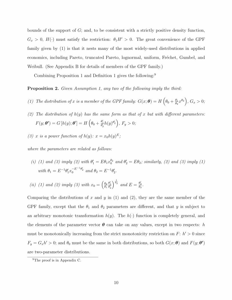
Proposition 1. Given Assumption 1, any two of the following imply the third:
(1) x is distributed with CDF G (x), where g(x) ≡ G′(x) > 0;
(2) y is distributed with CDF F (y), where f(y) ≡ F ′(y) > 0;
(3) Firm behavior, given technology and demand, is such that: x = v(y), v′(y) > 0;
7The assumption that they are increasing functions is without loss of generality. For example, if x(i)is increasing and y(i) is decreasing, Proposition 1 can easily be reformulated using the survival functionof y. Monotonicity here is a property of theoretical models. In our empirical applications we do not needto assume that any measured firm characteristics are monotonic in i. We follow standard models of firmheterogeneity under monopolistic competition by considering a continuum of firms whose characteristics arerealizations of a random variable. Because we work with a continuum, the c.d.f. of this random variable isthe actual distribution of these realizations. Henceforward, we use lower-case variables to describe both arandom variable and its realization.
8

where the functions are related as follows:
(i) (1) and (3) imply (2) with F (y) = G[v(y)] and f(y) = g[v(y)]v′(y); similarly, (2) and
(3) imply (1) with G(x) = F [v−1(x)] and g(x) = f [v−1(x)]d[v−1(x)]dx
.
(ii) (1) and (2) imply (3) with v(y) = G−1[F (y)].
Part (i) of the proposition is a standard result on transformations of variables. Part (ii) is
less standard, and requires Assumption 1: characteristics x(i) and y(i) must refer to the
same firm and must be monotonically increasing in i.8 The proof is in Appendix A. The
importance of the result is that it allows us to characterize fully the conditions under which
assumptions about distributions and about the functional forms that link them are mutually
consistent. Part (ii) in particular provides an easy way of determining which specifications
of firm behavior are consistent with particular assumptions about the distributions of firm
characteristics. All that is required is to derive the form of v(y) implied by any pair of
distributional assumptions.
Our next result shows how Proposition 1 is significantly strengthened when the distribu-
tions of the two firm characteristics share a common parametric structure, which is given by
the following:
Definition 1. A sub-family of probability distributions is a member of the “Generalized
Power Function” [“GPF”] family if there exists a continuously differentiable function H(·)
such that the cumulative distribution function of every member of the sub-family can be
written as:
G (x;θ) = H
(θ0 +
θ1
θ2
xθ2)
(1)
where each member of the sub-family corresponds to a particular value of the vector θ ≡
θ0, θ1, θ2.
The function H(·) is completely general, other than exhibiting the minimal requirements of
a probability distribution: G(xmin;θ) = 0 and G(xmax;θ) = 1, where xmin and xmax are the
8This implies that the Spearman rank correlation between x and y is one.
9
bounds of the support of G; and, to be consistent with a strictly positive density function,
Gx > 0, H(·) must satisfy the restriction: θ1H′ > 0. The great convenience of the GPF
family given by (1) is that it nests many of the most widely-used distributions in applied
economics, including Pareto, truncated Pareto, lognormal, uniform, Frechet, Gumbel, and
Weibull. (See Appendix B for details of members of the GPF family.)
Combining Proposition 1 and Definition 1 gives the following:9
Proposition 2. Given Assumption 1, any two of the following imply the third:
(1) The distribution of x is a member of the GPF family: G(x;θ) = H(θ0 + θ1
θ2xθ2)
, Gx > 0;
(2) The distribution of h(y) has the same form as that of x but with different parameters:
F (y;θ′) = G [h(y);θ′] = H(θ0 +
θ′1θ′2h(y)θ
′2
), Fy > 0;
(3) x is a power function of h(y): x = x0h(y)E;
where the parameters are related as follows:
(i) (1) and (3) imply (2) with θ′1 = Eθ1xθ20 and θ′2 = Eθ2; similarly, (2) and (3) imply (1)
with θ1 = E−1θ′1x−E−1θ′20 and θ2 = E−1θ′2.
(ii) (1) and (2) imply (3) with x0 =(θ2θ1
θ′1θ′2
) 1θ2 and E =
θ′2θ2
.
Comparing the distributions of x and y in (1) and (2), they are the same member of the
GPF family, except that the θ1 and θ2 parameters are different, and that y is subject to
an arbitrary monotonic transformation h(y). The h(·) function is completely general, and
the elements of the parameter vector θ can take on any values, except in two respects: h
must be monotonically increasing from the strict monotonicity restriction on F : h′ > 0 since
Fy = Gxh′ > 0; and θ0 must be the same in both distributions, so both G(x;θ) and F (y;θ′)
are two-parameter distributions.
9The proof is in Appendix C.
10

Each choice of the h(·) function generates in turn a further family, such that the trans-
formation h(y) follows a distribution from the GPF family.10 Proposition 2 shows that these
families are intimately linked via a simple power function that expresses one of the two firm
characteristics as a transformation of the other. In much of the paper we will concentrate
on two special forms for the h(·) function. The identity transformation, h(y) = y, implies
from Proposition 2 a property we call “self-reflection”, since the distributions of x and y are
the same. This case proves particularly useful when we consider distributions of firm sales
and output in Section 3. The other case we consider in detail is the odds transformation,
h(y) = y1−y , where 0 ≤ y ≤ 1. This implies a property we call “odds-reflection”, since the
distribution of y is an odds transformation of that of x. This case proves particularly useful
when we consider distributions of firm markups in Section 4.
In the next two sections we give some examples of links between distributions and models
of firm behavior implied by Propositions 1 and 2, with detailed derivations in Appendix F.
3 Backing Out Demands
The first set of applications of Proposition 2 apply part (ii) of the proposition: we ask what
demand functions are consistent with assumed distributions of two different firm attributes.
Moreover, following the existing literature, we ask when will we observe self-reflection, in
the sense that the distributions of the two attributes are the same (though with different
parameters of course). Figure 2 summarizes schematically the results of this section, which
specify the demand functions that are necessary and sufficient for self-reflection between the
distributions of any two of firm output x, sales revenue r, and productivity ϕ.
10Assuming that a transformation of a variable follows a standard distribution is a well-known method ofgenerating new functional forms for distributions. See Johnson (1949), who attributes it to Edgeworth, andJones (2015).
11

CEMR
r
CES
CREMR
x
Figure 2: Links Between Firm Characteristics
3.1 Self-Reflection of Productivity and Sales
We begin in this sub-section by focusing on the two central attributes of productivity and
sales revenue. We know from Helpman, Melitz, and Yeaple (2004) and Chaney (2008) that
CES demands are sufficient to bridge the gap between two Pareto distributions; and we also
know from Head, Mayer, and Thoenig (2014) that a lognormal distribution of productivity
coupled with CES demands implies a lognormal distribution of sales. We want to establish
the necessary conditions for these links, which in turn will tell us whether there are other
demand systems that ensure an exact correspondence between the form of the productivity
and sales distributions.
The answer to these questions is immediate from Proposition 2: if both productivity
ϕ and sales r follow the same distribution, which can be any member of the GPF family,
including the Pareto and the lognormal, then they must be related by a power function:
ϕ = ϕ0rE (2)
To infer the implications of this for demand, we use two properties of a monopolistically
competitive equilibrium. First, firms equate marginal cost to marginal revenue, so ϕ =
c−1 =(∂r∂x
)−1.11 Second, all firms face the same residual demand function, so firm sales
11Our approach does not require that the marginal costs be exogenous. They could be chosen endogenouslyby firms either by optimizing subject to a variable cost function, as in Zhelobodko, Kokovin, Parenti, andThisse (2012), or as the outcome of investment in R&D.
12

conditional on output are independent of productivity ϕ: r(x) = xp(x) and ∂r∂x
= r′(x).
Combining these with (2) gives a simple differential equation in sales revenue:
[r′(x)]−1 = ϕ0r(x)E (3)
Integrating this we find that a necessary and sufficient condition for self-reflection of pro-
ductivity and sales is that the inverse demand function take the following form:
p(x) =β
x(x− γ)
σ−1σ , 1 < σ <∞, x > γσ, β > 0 (4)
We are not aware of any previous discussion of the family of inverse demand functions in (4),
which expresses expenditure r(x) = xp(x) as a power function of consumption relative to a
benchmark γ. We detail its properties in Appendix D. Its key property, from (3), is that
the elasticity of marginal revenue with respect to total revenue is constant: E = 1σ−1
. Hence
we call it the “CREMR” family, for “Constant Revenue Elasticity of Marginal Revenue.” It
includes CES demands as a special case: when γ equals zero, (4) reduces to p(x) = βx−1σ ,
and the elasticity of demand is constant, equal to σ. More generally, the elasticity of demand
varies with consumption, ε(x) ≡ − p(x)xp′(x)
= x−γx−γσσ, though it approaches σ for large firms.
To give some intuition for the result that CREMR demands link GPF productivity and
sales, consider the Pareto case. A Pareto distribution of productivities ϕ implies that the
elasticity of the density of the productivity distribution is constant: if G(ϕ) is Pareto, so
G(ϕ) = 1 −(ϕϕ
)−k, with density function g(ϕ) = G′(ϕ), then the elasticity of density is
ϕg′(ϕ)g(ϕ)
= −(k+1). Similarly, a Pareto distribution of sales, r = px, implies that the elasticity
of the density of the sales distribution is constant: if F (r) = 1 −(rr
)−n, with density
function f(r) = F ′(r), then the elasticity of density is rf ′(r)f(r)
= −(n + 1). These two log-
linear relationships are only consistent with each other if demands also imply a log-linear
relationship between firm productivity and firm sales. In a Melitz-type model, productivity is
the inverse of marginal cost, which equals marginal revenue. Hence Pareto productivities and
13

Pareto sales are only consistent with each other if there is a log-linear relationship between
marginal and total revenue, which is the eponymous defining feature of CREMR demands.
To see this slightly more formally, suppose that the distribution of productivity is Pareto
with shape parameter k. Then for any two levels of productivity, c−11 and c−1
2 , the ratio
of their survival functions (one minus their cumulative probabilities) is(c2c1
)k. Since firms
are profit-maximizers, this is also the ratio of the survival functions of marginal revenues,[r′(x2)r′(x1)
]k. But if the elasticity of marginal revenue to sales revenue is constant and equal
to 1σ−1
, this in turn equals(r2r1
) kσ−1
. Since this is true for any arbitrary level of sales, it
implies that sales are distributed as a Pareto with scale parameter n = kσ−1
. This result
was derived for the case of Pareto productivities and CES demands by Chaney (2008). (See
also Helpman, Melitz, and Yeaple (2004).) The formal proof, a corollary of Proposition 2,
shows that it generalizes from CES to CREMR, and that GPF productivities and CREMR
demands are necessary as well as sufficient for this outcome.
x
p(x)
p
r'(x)
(a) γ = 0: CES
x
p(x)
p
r'(x)
(b) γ > 0: Subconvex
x
p(x)
p
r'(x)
(c) γ < 0: Superconvex
Figure 3: Examples of CREMR Demand and Marginal Revenue Functions
Figure 3 shows three representative inverse demand curves from the CREMR family, along
with their corresponding marginal revenue curves. The CES case in panel (a) combines
the familiar advantage of analytic tractability with the equally familiar disadvantage of
imposing strong and counter-factual properties. In particular, the proportional markup
pc
must be the same for all firms in all markets. By contrast, members of the CREMR
family with non-zero values of γ avoid this restriction. Moreover, we show in Appendix D
14

that the sign of γ determines whether a CREMR demand function is more or less convex
than a CES demand function. The case of a positive γ as in panel (b) corresponds to
demands that are “subconvex”: less convex at each point than a CES demand function
with the same elasticity. In this case the elasticity of demand falls with output, which
implies that larger firms have higher markups and that globalization has a pro-competitive
effect. These properties are reversed when γ is negative as in panel (c). Now the demands
are “superconvex” – more convex than a CES demand function with the same elasticity
– and larger firms have smaller markups. CREMR demands thus allow for a much wider
range of comparative statics responses than the CES itself. Finally, CREMR demands
can be rationalized by an additively separable utility function where the sub-utility is a
hypergeometric function. (For details, see Appendix E.) Since this is an analytic function,
CREMR demands can be used as a foundation for quantitative analysis of normative issues.
0.0
1.0
2.0
3.0
4.0
-2.0 -1.0 0.0 1.0 2.0 3.0
= 1.2
= 1.5
= 2 = 6 = 3SM CES
(a) CREMR Demands
0.0
1.0
2.0
3.0
4.0
-2.0 -1.0 0.0 1.0 2.0 3.0
Linear
CARAStone-Geary
TranslogCESSM
(b) Some Well-Known Demand Functions
Figure 4: Demand Manifolds for CREMR and Other Demand Functions
How do CREMR demands compare with other better-known demand systems? Inspect-
ing the demand functions themselves is not so informative, as they depend on three different
parameters. Instead, we use the approach of Mrazova and Neary (2013), who show that any
well-behaved demand function can be represented by its “demand manifold”, a smooth curve
relating its elasticity ε(x) ≡ − p(x)xp′(x)
to its convexity ρ(x) ≡ −xp′′(x)p′(x)
. We show in Appendix
15

D that the CREMR demand manifold can be written in closed form as follows:
ρ(ε) = 2− 1
σ − 1
(ε− 1)2
ε(5)
Whereas the demand function (4) depends on three parameters, the corresponding demand
manifold only depends on σ. Panel (a) of Figure 4 illustrates some manifolds from this
family for different values of σ, while panel (b) shows the manifolds of some of the most
commonly-used demand functions in applied economics: linear, CARA, Translog and Stone-
Geary (or Linear Expenditure System).12 It is clear that CREMR manifolds, and hence
CREMR demand functions, behave very differently from the others. The arrows in Figure
4 denote the direction of movement as sales increase. In the empirically relevant subconvex
region, where demands are less convex than the CES, CREMR demands are more concave
at low levels of output (i.e., at high demand elasticities) than any of the others, and their
elasticity of demand falls more slowly with convexity as sales rise.
3.2 CREMR and GPF Distributions: Some Special Cases
While the result of the previous sub-section holds for any distributions from the GPF family,
it is useful to consider in more detail the Pareto and lognormal cases. Starting with the
Pareto, since it is a member of the GPF family of distributions, it follows immediately as
a corollary of Proposition 2 that CREMR demands are necessary and sufficient for self-
reflection in this case. We state the result formally for completeness, and because it makes
explicit the links that must hold between the parameters of the two Pareto distributions and
12These manifolds are derived in Mrazova and Neary (2013). We confine attention to the admissible region,ε > 1, ρ < 2, defined as the region where firms’ first- and second-order conditions are satisfied. The curvelabeled “CES” is the locus ε = 1
ρ−1 , each point on which corresponds to a particular CES demand function;
this is also equation (5) with ε = σ. To the right of the CES locus is the superconvex region (where demandis more convex than the CES), while to the left is the subconvex region. The curve labeled “SM ” is thelocus ε = 3−ρ; to the right is the “supermodular” region (where selection effects in models of heterogeneousfirms have the conventional sign, e.g., more efficient firms serve foreign markets by foreign direct investmentrather than exports); while to the left is the submodular region. See Mrazova and Neary (2011) for furtherdiscussion.
16

the demand function. (In what follows we use r ∼ P(r, n) to indicate that r follows a Pareto
distribution with threshold parameter r and shape parameter n, so F (r) = 1−(rr
)−n.)
Corollary 1. Pareto Productivity and Sales Revenue: Any two of the following state-
ments imply the third: 1. Firm productivity ϕ ∼ P(ϕ, k); 2. Firm sales revenue r ∼ P(r, n);
3. The demand function belongs to the CREMR family in (4); where the parameters are
related as follows:
σ =k + n
n⇔ n =
k
σ − 1and β =
(k + n
k
rnk
ϕ
) kk+n
⇔ r = βσ(σ − 1
σϕ
)σ−1
(6)
Note that the demand parameter γ does not appear in (6), so these expressions hold for all
members of the CREMR family, including the CES. This confirms that Corollary 1 extends
a result of Chaney (2008), as noted earlier.
Although it has become customary to assume that actual firm size distributions can be
approximated by the Pareto, at least for larger firms, there are other candidate explanations
for the pattern of firm sales. Head, Mayer, and Thoenig (2014) and Bee and Schiavo (2014)
argue that firm size distribution is better approximated by a lognormal distribution than
a Pareto. We have already noted that the lognormal distribution is a special case of the
GPF family in Proposition 2. It follows immediately from the proposition that the CREMR
relationship ϕ = ϕ0rE is necessary and sufficient for self-reflection in the lognormal case.
However, unlike in the Pareto case, this does not imply that all CREMR demand functions
are consistent with lognormal productivity and sales. The reason is that, except in the CES
case (when the CREMR parameter γ is zero), the value of sales revenue for the smallest firm
is strictly positive.13 Strictly speaking, this is inconsistent with the lognormal distribution,
whose lower bound is zero. We can summarize this result as follows. (We use r ∼ LN (µ, s)
to indicate that r follows a lognormal distribution with location parameter µ and scale
13Since p′(x) = − βσx2 (x− γ)−
1σ (x− γσ), the output of the smallest firm when γ is strictly positive is γσ,
while its sales revenue is r(x) = β [γ(σ − 1)]σ−1σ > 0. When demands are strictly superconvex, so γ is strictly
negative, sales revenue is discontinuous at x = 0: limx→0+
r(x) = β(−γ)σ−1σ > 0, but r(0) = 0.
17

parameter s, equal to the mean and standard deviation of the natural logarithm of r. Hence
F (r) = Φ(
log r−µs
), where Φ is the cumulative distribution function of the standard normal
distribution.)
Corollary 2. Lognormal Productivity and Sales Revenue: Any two of the following
statements imply the third: 1. Firm productivity follows a LN (µ, s) distribution; 2. Firm
sales follow a LN (µ′, s′) distribution; 3. The demand function is CES: p(x) = βx−1σ ; where
the parameters are related as follows:
σ =s+ s′
s⇔ s′ = (σ−1)s and β =
s+ s′
s′exp
( ss′µ′ − µ
)⇔ µ′ = (σ−1)
[µ+ log
(β
σ
)](7)
Hence, unlike the Pareto case, the only demand function that is exactly compatible with
lognormal productivity and sales is the CES. Relaxing the assumption of Pareto productivity
in favor of lognormal productivity comes at the expense of ruling out pro-competitive effects.
However, in practical applications, where there is a finite interval between the output of the
smallest firm and zero, we may not wish to rule out combining lognormal productivity with
members of the CREMR family other than the CES.
3.3 Self-Reflection of Productivity and Output
The distribution of sales revenue is not the only outcome predicted by models of heteroge-
neous firms. We can also ask what are the conditions under which output follows the same
distribution as productivity. Proposition 2 implies that a necessary and sufficient condition
for this form of self-reflection is that the elasticity of productivity with respect to output be
constant. This turns out to be related to a different demand family:
p(x) =1
x(α + βx
σ−1σ ) (8)
18
The demand function in (8) plays the same role with respect to the characteristic of interest,
in this case firm output, as the CREMR family does with respect to firm sales. It is necessary
and sufficient for a constant elasticity of marginal revenue with respect to output, equal to
1σ. Hence we call it “CEMR” for “Constant (Output) Elasticity of Marginal Revenue.”14
Unlike CREMR, there are some precedents for this class. It has the same functional
form, except with prices and quantities reversed, as the direct PIGL (“Price-Independent
Generalized Linearity”) class of Muellbauer (1975).15 In particular, the limiting case where
σ approaches one is the inverse translog demand function of Christensen, Jorgenson, and
Lau (1975). However, except for the CES (the special case when α = 0), CEMR demands
bear little resemblance to commonly-used demand functions.16
When the common distribution of productivity and output is a Pareto, we can immedi-
ately state a further corollary of Proposition 2:
Corollary 3. Pareto Productivity and Output: Any two of the following statements
imply the third: 1. Firm productivity ϕ ∼ P(ϕ, k); 2. Firm output x ∼ P(x,m); 3. The de-
mand function belongs to the CEMR family (8); where the parameters are related as follows:
σ =k
m⇔ m =
k
σand β =
k
k −mxmk
ϕ⇔ x =
(βσ − 1
σϕ
)σ(9)
However, when both productivity and output follow a lognormal distribution, we en-
counter a similar though less extreme restriction on the range of admissible CEMR demand
functions to that in the CREMR case of Corollary 2. Now the requirement that output be
zero for the smallest firm is only possible if both the parameters α and β in the CEMR
demand function (8) are positive. As shown by Mrazova and Neary (2013), this corresponds
14“CEMR” rhymes with “seemer.”15For this reason, Mrazova and Neary (2013) called it the “inverse PIGL” class of demand functions.16As shown by Mrazova and Neary (2013), the CEMR demand manifold implies a linear relationship
between the convexity and elasticity of demand, passing through the Cobb-Douglas point (ε, ρ) = (1, 2):ρ = 2 − ε−1
σ . The manifold for the inverse translog special case (σ → 1) coincides with the SM locus inFigure 4(b). For high elasticities (corresponding to small firms when demand is subconvex), CEMR demandsare qualitatively similar to CREMR, except that they are somewhat more elastic: the CEMR manifold canbe written as ε = (2− ρ)σ + 1, while for high ε the CREMR manifold becomes ε = (2− ρ)(σ − 1) + 1.
19

to the case where CEMR demands are superconvex. By contrast, if either α or β is strictly
negative, then demands are strictly subconvex: more plausible in terms of its implications
for the distribution of markups, but not compatible with a lognormal distribution of output.
Summarizing:
Corollary 4. Lognormal Productivity and Output: Any two of the following state-
ments imply the third: 1. Firm productivity follows a LN (µ, s) distribution; 2. Firm output
follows a LN (µ′, s′) distribution; 3. The demand function belongs to the superconvex sub-
class of the CEMR family (8) with α ≥ 0, β ≥ 0, and αβ > 0; where the parameters are
related as follows:
σ =s′
s⇔ s′ = σs and β =
s′
s′ − sexp
( ss′µ′ − µ
)⇔ µ′ = σ
[µ+ log
(βσ − 1
σ
)](10)
3.4 Self-Reflection of Output and Sales
A final self-reflection corollary of Proposition 2 relates to the case where output and sales
follow the same distribution. This requires that the elasticity of one with respect to the
other is constant, which implies that the demand function must be a CES.17 Formally:
Corollary 5. Pareto Output and Sales Revenue: Any two of the following statements
imply the third: 1. The distribution of firm output x is a member of the generalized power
function family; 2. The distribution of firm sales revenue r is the same member of the
generalized power function family; 3. The demand function is CES: p(x) = βx−1σ , where
β = x− 1E
0 and σ = EE−1
.
In the Pareto case, the sufficiency part of this result is familiar from the large literature
on the Melitz model with CES demands: it is implicit in Chaney (2008) for example. The
necessity part, taken together with earlier results, shows that it is not possible for all three
17Suppose that x = x0r(x)E . Recalling that r(x) = xp(x), it follows immediately that the demand functionmust take the CES form.
20

firm attributes, productivity, sales and revenue, to have the same distribution from the
generalized power family class under any demand system other than the CES. Corollary 5
follows immediately from previous results when productivities themselves have a generalized
power function distribution, since the only demand function which is a member of both the
CEMR and CREMR families is the CES itself. However, it is much more general than that,
since it does not require any assumption about the underlying distribution of productivities.
It is an example of a corollary to Proposition 2 which relates two endogenous firm outcomes
rather than an exogenous and an endogenous one. Taken together, the results of this section
show that exactly matching a Pareto or lognormal distribution of firm sales or output, when
productivity is assumed to have the same distribution, places strong restrictions on the
admissible demand function. The elasticity of marginal revenue with respect to the firm
outcome of interest must be constant, and the implied demand function must be consistent
with the range of the distribution assumed. However, that leaves open the question of how
great an error would be made by using a demand function which does not allow for an exact
fit. We address this question in Section 5. First, we turn to consider the implications of
different demand functions for the distributions of sales and markups.
4 Inferring Sales and Markup Distributions
The previous section used part (ii) of Proposition 2 to back out the demands implied by
assumed distributions of two firm characteristics. In this section we show how part (i) can be
used to derive the distributions of firm characteristics given the distribution of productivity
and the form of the demand function. Section 4.1 considers the distributions of markups
implied by CREMR demands, while Section 4.2 presents the distributions of both sales and
markups implied by a number of widely-used demand functions.
21

4.1 CREMR Markup Distributions
We begin with the case of CREMR demands, since they imply a particularly simple form
for the markup distribution. In order to be able to invoke Proposition 2, we need to express
productivity as a function of the markup.
The first step is to express output as a function of the markup. In general, with the
markup m defined as pc, we can write the markup as a function of output by invoking a
standard expression in terms of the elasticity of demand: m(x) = ε(x)ε(x)−1
. Specializing to the
case of CREMR demands, recall from Section 3.1 that the elasticity of demand for CREMR
demand functions is ε(x) = x−γx−γσσ. Hence, we can write the CREMR markup as a function
of output: m(x) = x−γx
σσ−1
. We concentrate on the case of subconvex demands (i.e., γ > 0),
which implies that larger firms have higher markups: m(x) ∈[m, σ
σ−1
]as x ∈ [x,∞]. Define
the relative markup as the markup relative to its maximum value, σσ−1
, which is the value
that obtains under CES preferences with the same value of σ: m ≡ mm
= σ−1σm ∈ [m, 1].
Hence it follows that: m(x) = x−γx
. Inverting this allows us to express output as a function
of the relative markup: x(m) = γ1−m .
The next step is to express productivity ϕ as a function of output. This follows from
profit-maximization, which implies that marginal cost ϕ−1 equals marginal revenue, given
by equation (22) in Appendix D: ϕ(x) = 1β
σσ−1
(x− γ)1σ . Finally, combining ϕ(x) and x(m),
gives the desired relationship between productivity and the markup:
ϕ(m) = ϕ0
(m
1− m
) 1σ
ϕ0 ≡1
β
σ
σ − 1γ
1σ (11)
Clearly this satisfies Proposition 2’s conditions for “Odds Reflection”. Hence, if productivity
follows any distribution in the GPF class, and if the demand function belongs to the sub-
convex CREMR family, equation (4) with γ > 0, then Proposition 2 implies that markups
follow the corresponding “GPF-odds” distribution.
Once again, we focus on three particularly interesting cases:
22

Introduction From theory to data Empirics
Logit-normal
Figure 5: The Lognormal-Odds Distribution
1. Pareto: If demands are subconvex CREMR and productivity ϕ is distributed as a
Pareto, so G(ϕ) = 1− ϕkϕ−k, then the relative markup must follow a “Pareto-Odds”
distribution:
F (m) = 1−(
m
1− m
)n′ (m
1− m
)−n′m ∈ m, 1 m ≡ m
m, m ≡ m
m. (12)
where n′ ≡ kσ
and m ≡ ϕσ
ϕσ+ϕσ0
. This distribution appears to be new, and may prove
useful in future applications. However, it implies that the distribution of markups
is U-shaped, which is less in line with the available evidence than the next case we
consider, although the minimum value of the U may lie to the left of the relevant [0, 1]
interval.
2. Lognormal: If demands are subconvex CREMR and productivity follows a lognormal
distribution, so G(ϕ) = Φ[
1slogϕ− µ
], then the relative markup must follow a
“Lognormal-Odds” distribution:
F (m) = Φ
[1
s′
log
m
1− m− µ′
](13)
where: s′ ≡ σs and µ′ ≡ σ(µ − logϕ0). This distribution has been studied in the
statistics literature where it is known as the “Logit-Normal”, though we are not aware
of a theoretical rationale for its occurrence as here.18 Figure 5 illustrates some mem-
18See Johnson (1949) and Mead (1965).
23

bers of this family of distributions. Comparing these with the empirical results from
De Loecker, Goldberg, Khandelwal, and Pavcnik (2016) and Lamorgese, Linarello,
and Warzynski (2014) illustrated in Figure 1, which also exhibit inverted-U-shaped
profiles, suggests that the lognormal-odds distribution provides a good fit for the em-
pirical markup distribution. Of course, a more precise way of measuring goodness of
fit of distributions would be preferable; we will turn to this in the next section.
3. Frechet: Finally, if productivity follows a Frechet distribution and demands are CREMR,
then the relative markup must follow a “Frechet-Odds” distribution. Once again, this
distribution appears to be new. It provides an exact characterization of the distribution
of profit margins for a firm that sells in many foreign markets, where the distribution
of productivity draws across markets follows a Frechet distribution, as in Tintelnot
(2017).
4.2 Other Sales and Markup Distributions
p(x) or x(p) ϕ(r) or ϕ(r) ϕ(m) or ϕ(m)
CREMR βx (x− γ)
σ−1σ ϕ0r
1σ−1 ϕ0
(m
1−m
) 1σ
Linear α− βx 1α
(1
1−r
) 12 2m−1
α
LES δx+γ γδ
(1
1−r
)2γδm
2
Translog/AI 1p (γ − η log p) ϕ0(r + η) exp
(rη
)m exp
(m− η+γ
η
)Table 1: Productivity as a Function of Sales and Markups
for Selected Demand Functions
Proposition 2 can be used to derive the distributions of sales and markups implied by any
demand function. In particular, closed-form expressions for productivity as a function of sales
or markups can be derived for some of the most widely-used demand functions in applied
24

economics. Table 1 gives results for linear, Stone-Geary or linear expenditure system (LES),
and translog demands, along with the CREMR results already derived.19 Combining these
with different assumptions about the distribution of productivity, and invoking Proposition
2, it is clear that a wide variety of sales and markup distributions are implied.20 For example,
the relationships between productivity and sales implied by linear and LES demands have
the same form, so the sales distributions implied by these two very different demand systems
are observationally equivalent. The same is not true of their implied markup distributions,
however: in the LES case, productivity is a simple power function of markups, so the LES
implies self-reflection of the productivity and markup distributions if either is a member of
the GPF class.21
It is clearly desirable to compare the distributions implied by these different demand
functions with each other and with a given empirical distribution. In the remainder of the
paper we turn to this task.
5 Comparing Predicted and Actual Distributions
5.1 From Theory to Calibration
So far we have characterized the exact distributions of firm size and firm markups implied
by particular assumptions about the primitives of the model: the structure of demand and
the distribution of firm productivities. Results of this kind provide an essential benchmark,
but they are not so helpful from a quantitative perspective: they do not tell us by how much
a theoretically-implied distribution departs from a given distribution, whether hypothetical
19From a firm’s perspective, the translog is observationally equivalent to the almost ideal (AI) model ofDeaton and Muellbauer (1980).
20For parameter restrictions and other details, such as the form of ϕ0 (which differs in each case), seeAppendix G. Note that in some cases it is desirable to express the results in terms of sales relative to themaximum level, r ≡ r
r , just as with CREMR demands the markup distribution is most easily expressed interms of the relative markup m.
21For example, a lognormal distribution of productivity and LES demand imply a lognormal distributionof markups, so providing microfoundations for an assumption made by Epifani and Gancia (2011).
25

or observed. In the remainder of the paper, we turn to explore the quantitative implications
of our approach when applied to actual data sets. In particular, we quantify the differences
between the actual distributions in the data and a variety of distributions implied by different
theoretical models. To measure the “goodness of fit” of different models, we use the Kullback-
Leibler divergence (denoted “KLD” hereafter), introduced by Kullback and Leibler (1951).
We also present results for the QQ estimator as a robustness check.22 The next sub-section
sketches the theoretical properties of the KLD, while Section 5.3 shows how we operationalize
it. To fix ideas, we focus on explaining the distribution of firm sales. Adapting the framework
to explain the distribution of output, markups, or any other firm outcome, is straightforward.
5.2 The Kullback-Leibler Divergence
The KLD measures the “information loss” or “relative entropy” when one distribution, F ,
is used to approximate another, F :
DKL(F ||F (.;θ)) ≡∫ r
r
log
(f(r)
f(r;θ)
)f(r)dr (14)
In our context, the observed distribution F (r) is the actual distribution of firm sales. As
for F (r;θ), it is the distribution of firm sales implied by the underlying distribution of firm
productivities, G(ϕ), combined with a model of firm behavior, ϕ(r;θ), parameterized by θ.
The KLD has a number of desirable features, the first two of which are well-known. First,
it has an axiomatic foundation in information theory: we give further details in Appendix
H.1. Second, it has an elegant statistical interpretation: it equals the expected value of
the inverse log-likelihood ratio, so choosing the parameter vector θ to minimize the KLD
22Other criteria could be used, though none is as satisfactory as the KLD. A first- or second-order stochasticdominance criterion is not informative about the dissimilarity between the two firm size distributions if theircumulative distributions intersect more than once. The Kolmogorov-Smirnov test privileges the maximumdeviation between the two cumulative distributions, and ignores information about the distributions atother points. As for matching moments, this does not guarantee a close fit unless many moments are used.Moreover, there is a specific problem with matching moments for the Pareto distribution. The t’th momentexists if and only if the dispersion parameter k exceeds t; however, empirically, raw data often exhibit valuesof k that are less than one, so even the mean does not exist.
26

is asymptotically equivalent to maximizing the likelihood. Third, and new in this paper,
is that it links directly with Proposition 2: the KLD in our context can be decomposed to
show how it relates to the Revenue Elasticity of Marginal Revenue (REMR) E:
DKL(F ||F (.;θ)) = log f(r)− log
[g (ϕ(r))
dϕ
dr
∣∣∣∣r
]︸ ︷︷ ︸
(1)
+
∫ r
r
1− F (r)
r
[rf ′(r)
f(r)+ 1
−ϕg′(ϕ(r))
g(ϕ(r))+ 1
E(r)︸ ︷︷ ︸
(2)
− rE ′(r)
E(r)︸ ︷︷ ︸(3)
]dr
(15)
Recall that Proposition 2 derived necessary and sufficient conditions for an exact match
between the distributions of two firm characteristics when both distributions belong to the
same member of the generalized power function family: the elasticity of one characteristic
with respect to the other should be constant, and its value should be consistent with the
parameters of the two distributions. Equation (15) goes further and quantifies the infor-
mation loss when the assumptions of Proposition 2 do not hold. In particular, it identifies
three distinct sources of information loss in matching a fitted distribution F (r) to an actual
distribution of firm sizes F (r). First is a failure to match the lower end-point of the distri-
bution, r. Second is a mismatch at each point in the range between the actual elasticity of
density of the firm size distribution, rf ′(r)f(r)
, and that predicted by the assumptions about the
productivity distribution and the REMR, ϕg′(ϕ(r))g(ϕ(r))
E(r). And third is a failure to allow for
variations in the REMR E; i.e. a failure to allow for deviations from part (iii) of Proposi-
tion 2. Each of these three components can be positive or negative, but their sum must be
non-negative. Appendices H.2 and H.3 give details and applications.
5.3 Operationalizing the KLD
To compare the fit of predicted and actual distributions we use the discrete counterpart
of the continuous KLD introduced in Section 5.2. We choose the parameter vector θ to
27

minimize the KLD between the empirical c.d.f. F defined over the support [r, r], and the
theoretical c.d.f. F (.;θ). Considering the histogram corresponding to F , defined over nb bins
with width equal to b, the KLD becomes:
DKL(F || F (.;θ)) =nb∑i=1
(F (r + i ∗ b)− F (r + (i− 1) ∗ b)) log(F (r+i∗b)−F (r+(i−1)∗b)F (r+i∗b)−F (r+(i−1)∗b)
) (16)
We report below DKL(F || F (.; θ)), where θ is the parameter vector that minimizes DKL(F ||
F (.;θ)).
In the next section, we set the number of bins equal to 1, 000. Fortunately, the ranking
of different models is not very sensitive to the number of bins considered. When the number
of bins increases without bound, our estimator is asymptotically equivalent to the maximum
likelihood estimator under the additional constraint that the empirical support of the distri-
bution is included in the one predicted by the theory.23 As for the units of measurement for
the KLD, information scientists typically present values in “bits” (log to base 2) or “nats”
(log to base e). Such units have little intuitive appeal in economics. Instead, we present
the values of the KLD normalized by the value implied by a uniform distribution of sales.24
This is an uninformative prior in the spirit of the “dartboard” approach to benchmarking
the geographic concentration of manufacturing industry of Ellison and Glaeser (1997), or
the “balls and bins” approach to benchmarking the world trade matrix of Armenter and
Koren (2014). The value of the KLD is unbounded, but a specification that gave a value
greater than that implied by a uniform distribution could not be considered a satisfactory
explanation of the data.
23When the distribution is lognormal this difference is immaterial as the support consists of R+. This isno longer the case when the distribution is Pareto.
24See (37) in Appendix H.1 for the explicit expression.
28

6 Empirical Applications
To illustrate how the KLD can be used to compare the goodness of fit of different assumptions
about demand and the distribution of productivity, we end with two empirical applications.
The first, in Section 6.1, uses data on French exports to Germany in 2005, drawn from the
same source as that used by Head, Mayer, and Thoenig (2014). The second, in Section
6.2, uses firm-level data on Indian sales and markups, as used by De Loecker, Goldberg,
Khandelwal, and Pavcnik (2016). Section 6.3 explores how robust are the results with Indian
data to dropping smaller observations. Finally, as a further robustness check, Section 6.4
confirms that an alternative criterion for choosing between distributions, the QQ estimator,
give qualitatively similar results to the KLD.
6.1 French Exports to Germany
(a) A First Look: Obviously Pareto?
(1) (2) (3)
(b) A Second Look: Obviously Lognormal?
Figure 6: Alternative Perspectives on the Data
The data consists of the universe of French exports to Germany in 2005.25 Figure 6 shows
that the data exhibit some typical features of such data sets. When we plot a histogram
with the log frequency on the vertical axis and actual sales on the horizontal, as in Panel
25It contains 161,191 firm-product observations on export sales by 27,550 firms: 5.85 products per firm.We are very grateful to Julien Martin for performing the analysis for us on French Customs data.
29

(a), the long tail is clearly in evidence, and it seems plausible that the data are generated by
a Pareto distribution. However, the first bin contains over half the firms, which is brought
out more clearly when we plot the actual frequency on the vertical axis and log sales on
the horizontal, as in Panel (b). Now the data seem self-evidently lognormal. Yet a third
perspective comes from the vertical lines in Panel (b). The line labeled (1) is at median
sales, with 50% of firms to the left, but these account for only 0.1% of sales; the line labeled
(2) is at 76.7% of firms, but these account for only 1.0% of sales; finally, the line labeled
(3) is at 99.6% of firms, which account for only 50% of sales. Thus, we might reasonably
conclude that the data are Pareto where it matters, with the top firms dominating.
0 0.5 1 1.5 2 2.5 3 3.5 4
x 109
(a) All Observations
0 1 2 3 4 5 6
x 107
(b) All Bar Top 89 Observations
Figure 7: KLD-Minimizing Predicted Distributions: Pareto (green) and Lognormal (red)
These subjective considerations provide a poor basis for discriminating between rival
views of the best underlying distribution, and justify our turning to use the KLD as a more
objective indicator of how well different assumptions fit the data. Figure 7 compares the
best-fit Pareto (in green) and lognormal (in red). From Section 3, each of these amounts to
assuming that demand is CREMR, and that the underlying productivity distribution is either
Pareto or lognormal. (Note that the distribution and demand parameters are not separately
identified.) In each case, we choose parameter values for the specification in question that
minimize the KLD: recall that this is asymptotically equivalent to a maximum likelihood
30

estimation of those parameters, conditional on the specification. Panel (a) illustrates the
results for all firms, while panel (b) avoids the distorted perspective caused by including the
largest firms, by omitting the top 89 firms, which account for 0.05% of observations but 32%
of sales. Inspecting the fitted distributions, it is evident that the lognormal matches the
smaller firms better, and conversely for the Pareto. The values of the minimized KLD show
that the lognormal provides a better overall fit than the Pareto: 0.0001 as opposed to 0.0012.
(Recall that the data are normalized by the value of the KLD for a uniform distribution,
which for this data set is 6.8082.)
CREMR/CES Translog/AI Linear and LES
Pareto 0.0012 0.3819 0.4711Lognormal 0.0001 0.7315 0.8314
Table 2: KLD for French Exports Compared with Predictions fromSelected Demand Functions and Productivity Distributions
Table 2 gives the values of the KLD for the Pareto and lognormal cases shown in Fig-
ure 7, and also for the distributions implied by either translog or linear demand functions
combined with either Pareto or lognormal productivities. These distributions are calculated
by combining the relevant productivity distribution with the relationships between produc-
tivity and sales implied by translog and linear demands from Table 1. (Recall from that
table that the linear and LES specifications are observationally equivalent.) Each entry in
the table is the value of the KLD that measures the information loss when the combination
of assumptions indicated by the row and column is used to explain the observed distribution
of sales.
To assess whether the values are significantly different from one another, we use a boot-
strapping approach. We construct one thousand samples of the same size as the data (i.e.,
161,191 observations), by sampling with replacement from the original data. For each sam-
ple, we then compute the KLD value for each of the six models. Table 3 gives the results.
Each entry in the table is the proportion of samples in which the combination in the relevant
31

column gives a higher value of the KLD than that in the relevant row. All the values are
equal to or very close to 100%, which confirms that the results in Table 2 are robust.
CREMR + LN CREMR + P TLog + P Lin + P TLog + LN Lin + LN
CREMR + LN – 0% 0% 0% 0% 0%CREMR + P 100% – 0% 0% 0% 0%
TLog + P 100% 100% – 0% 0% 0%Lin + P 100% 100% 100% – 0% 0%
TLog + LN 100% 100% 100% 100% – 0.3%Lin + LN 100% 100% 100% 100% 99.7% –
Table 3: Bootstrapped Robustness of the KLD Ranking: French Sales(See text for explanation)
Turning to the results in Table 2, recall that panel (a) of Figure 7 showed that the
lognormal matches the smaller firms better, and conversely for the Pareto. Table 2 provides
a quantitative confirmation of this. With a preponderance of the bins corresponding to
smaller firms, it is not surprising that the lognormal does better as measured by the KLD:
as shown in the second column, it yields a value of 0.0017, considerably lower than the
value of 0.0090 for the Pareto. However, the difference between distributions turns out to be
much less significant than that between different specifications of demand. The KLD values
for the translog/AI and linear/LES specifications are much higher than for the CREMR
case, as shown in the third and fourth columns of Table 2, with the Pareto now preferred
to the lognormal. The overwhelming conclusion from these results is that, if we want to
fit the distribution of sales in this data set, then the choice between Pareto and lognormal
distributions is less important than the choice between CREMR and other demands.
6.2 Indian Sales and Markups
The second data set we use has 2,457 firm-product observations on both sales and markups
in Indian manufacturing for the year 2001. (See De Loecker, Goldberg, Khandelwal, and
Pavcnik (2016) for a detailed description of the data, which come from the Prowess data
set collected by the Centre for Monitoring the Indian Economy (CMIE).) While the sales
32

CREMR Translog/AI LES Linear
A. SalesPareto 0.2253 0.1028 0.1837 0.1837Lognormal 0.0140 0.5825 0.7266 0.7266
B. MarkupsPareto 0.1851 0.2205 0.2191 0.2512Lognormal 0.1863 0.2228 0.2083 0.2075
Table 4: KLD for Indian Sales and Markups Compared with Predictions fromSelected Demand Functions and Productivity Distributions
data are directly observed, the markup data are estimated, using the so-called “production
approach”. This approach relies solely on cost-minimization: markups are calculated by
computing the gap between the output elasticity with respect to variable inputs and the share
of those inputs in total revenue. It is particularly well-suited to our purposes, since it does
not impose any restrictions on consumer demand and is consistent with a variety of market
structures including monopolistic competition. Since the empirical markup distribution has
been obtained without making any assumption about functional forms, we can therefore
compare objectively the performance of different productivity distributions combined with
different demand systems based on the distributions of sales and markups that they imply.
The empirical markup distribution was shown in Figure 1(a) above. Observations with
negative markups (about 20% of the total) are not included in the sample, as they are
inconsistent with steady-state equilibrium behavior by firms. The remaining observations
are demeaned by product-year and firm-year fixed effects, so the sample mean equals one by
construction.
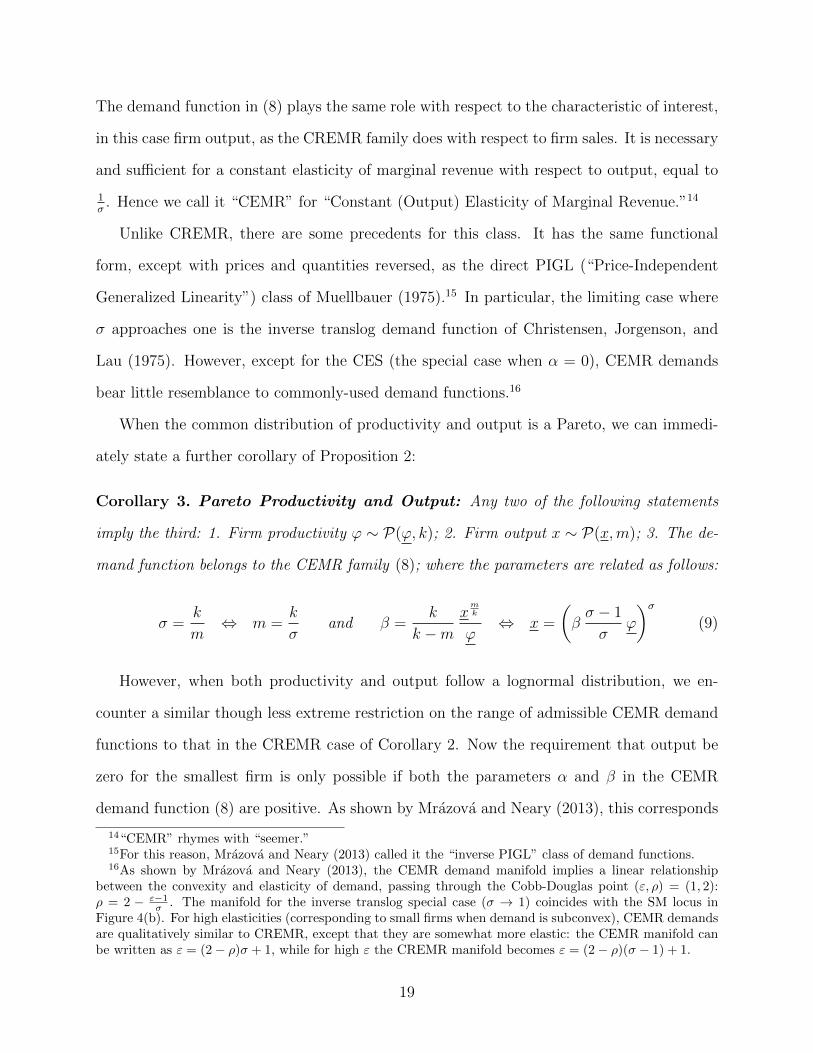
The KLD results are given in Table 4 and illustrated in Figure 8. As with the French
data, these results are normalized by the KLD for a uniform distribution, and bootstrapping
confirms that the differences between them are highly robust. (Appendix I gives details.)
The KLD values for sales are broadly in line with those from the French data. The one
major difference is that, conditional on a Pareto distribution of productivities, CREMR
33
KLD (Sales)
KLD(Markups)
CREMR
TranslogTranslog
LESLES
Linear
Linear
CREMR
0.18
0.20
0.22
0.24
0.26
0.00 0.10 0.20 0.30 0.40 0.50 0.60 0.70 0.80
Lognormal Productivity
Pareto Productivity
Figure 8: KLD for Indian Sales and Markups
demands give the worst fit to sales, with translog demands performing best, and linear-LES
intermediate between the others. However, the differences between the KLD values for these
specifications are much less than those conditional on lognormal productivities. Here the
ranking is the same as with the French data: CREMR does best, with translog performing
much less well and Linear-LES worst of all.
Of most interest are the results for markups. Here CREMR demands clearly do best,
irrespective of the assumed distribution, with translog and LES performing at the same level,
and linear doing equally well under Pareto assumptions but less well in the lognormal case.
(Recall from Table 1 that linear and LES demands are not separately identified for sales, but
they are for markups.) These results for markups reinforce the finding from the French data
that the choice between Pareto and lognormal distributions is less important than the choice
between CREMR and other demands. For sales a similar pattern applies conditional on
lognormal productivity, whereas in the Pareto case the choice of demand is less important,
with CREMR doing worst of all.
34
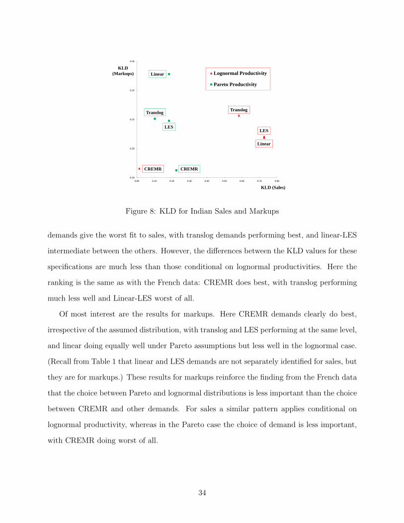
6.3 Robustness to Truncation
As we have seen in the two preceding sub-sections, the results with French and Indian
sales data are very similar, except for the case of CREMR demands combined with Pareto
productivity: this gives a good fit with French data but performs less well with Indian data.
One possible explanation for this is that the French data relate to exports, whereas the Indian
data are for total domestic production. Presumptively, smaller firms have been selected out
of the French data, so we might expect the Pareto assumption to be more appropriate. To
throw light on this issue, we explore the robustness of the Indian results to left-truncating
the data: specifically, we repeat a number of the comparisons between different specifications
for the Indian sales distribution dropping one observation at a time.
KLD
Number of Observations Dropped
0.00
0.05
0.10
0.15
0.20
0.25
0 200 400 600 800
Pareto + CREMR
Lognormal + CREMR
Figure 9: CREMR vs. CREMR: KLD for Indian Sales
Table 9 compares the KLD for the Pareto and lognormal, conditional on CREMR de-
mands, starting on the left-hand side with all observations (so the values are the same as in
Figure 8) and successively dropping up to 809 observations.26 Although the curves are not
26Each KLD value is normalized by the value of the KLD for a uniform distribution corresponding to thenumber of observations dropped. Alternative approaches would make very little difference however, as theKLD value for the uniform varies very little, from 3.9403 with no observations dropped to 3.5598 with 809observations dropped.
35

precisely monotonic, the broad picture is clear: conditional on CREMR demands, Pareto
does better and lognormal does worse as more and more observations are dropped. The
Pareto specification dominates when we drop 663 or more observations: these account for
27% of all firm-product observations, but only 1.2% of total sales.
0.00
0.05
0.10
0.15
0.20
0.25
0 20 40 60 80 100 120 140 160 180 200
Pareto + CREMR
Pareto + Linear/LES
Pareto + Translog
KLD
Number of Observations Dropped
Figure 10: CREMR vs. The Rest, Given Pareto: KLD for Indian Sales
Figure 10 shows that a similar pattern emerges when we compare the performance of
different demand functions in explaining the sales distribution, conditional on a Pareto dis-
tribution for productivity. In this case, the CREMR specification overtakes the linear one
when we drop 11 or more observations, which account for 0.44% of all firm-product observa-
tions, and only 0.0002% of sales. While it overtakes the translog when we drop 118 or more
observations, which account for 4.80% of observations, and 0.03% of sales.
These findings confirm that both CREMR and Pareto fit the sales data relatively better
when the smallest observations are dropped. They also make precise the pattern observed
in Figure 6 and in many other datasets: the right tail of the sales distribution, where the
Pareto assumption outperforms the lognormal, begins at exactly 663 observations.
36

6.4 Robustness: The QQ Estimator
A different kind of robustness check is to consider an alternative criterion to the KLD for
comparing predicted and actual distributions. Here we consider the QQ estimator, developed
by Kratz and Resnick (1996), and previously applied by Head, Mayer, and Thoenig (2014)
and Nigai (2017). Unlike the KLD, this estimator does not have a maximum likelihood
interpretation. However, it is more intuitive, since the QQ distance measure is simply the
sum of the squared deviations of the quantiles of the predicted distribution from those of
the actual distribution:
QQ(F || F (·;θ)) =n∑i=1
(log qi − log qi(θ))2 (17)
where qi = F−1(i/n) is the i’th quantile observed in the data, while qi(θ) = F−1(i/n;θ) is
the i’th quantile predicted by the theory. The QQ estimator θ is defined as the parameter
vector that minimizes the sum of squares QQ(F || F (·;θ)) in (17).
CREMR Translog LES Linear
A. SalesPareto 58.939 12.693 24.484 24.484Lognormal 3.078 116.918 133.274 133.274
B. MarkupsPareto 0.113 0.978 1.133 3.606Lognormal 0.110 0.990 0.340 0.325
Table 5: QQ Estimator for Indian Sales and Markups
To implement the QQ estimator we need analytic expressions for the quantiles under each
of the eight combinations of assumptions about demand and the distribution of productivity
we consider. These are given in Appendix J. We set the number of quantiles n equal to 100.
The resulting values of the QQ estimator for Indian sales and markups are given in Table 5,
and they are illustrated in Figure 11. As with the KLD values in Section 6.2, we scale these
37

0.00
0.50
1.00
1.50
2.00
2.50
3.00
3.50
4.00
0.0 20.0 40.0 60.0 80.0 100.0 120.0 140.0
Lognormal Productivity
Pareto Productivity
QQ (Sales)
QQ(Markups)
CREMR
Translog
Translog
LES
LES
Linear
Linear
CREMR
Figure 11: QQ Estimator for Indian Sales and Markups
by the uniform benchmark, which is 2.420 for sales and 90.133 for markups.
Comparing Table 5 with Table 4, and Figure 11 with Figure 8, it is evident that the
results based on the QQ estimator are qualitatively very similar to those for the KLD. In
particular, the Pareto assumption gives a better fit for sales than for markups, except in
the CREMR case; while the lognormal assumption tends to give a better fit for markups
than for sales. Comparing different demand functions, CREMR demands give a better
fit to the markup distribution than any other demands, irrespective of which productivity
distribution is assumed. As for sales, the results differ between the Pareto and lognormal
cases. Conditional on lognormal, CREMR again performs much better, whereas, conditional
on Pareto, it performs least well, with the translog doing best. The only qualitative difference
between the results using the two criteria is that with the QQ estimator the translog does
somewhat better than the LES in fitting the markup distribution. Overall, we can conclude
that the rankings given earlier are not unduly sensitive to our choice of criterion for comparing
actual and predicted distributions.
38

7 Conclusion
This paper has addressed the question of how to explain the distributions of firm size and
firm markups using models of heterogeneous firms. We provide a general necessary and
sufficient condition for consistency between arbitrary assumptions about the distributions
of two firm characteristics and an arbitrary model of firm behavior which relates those two
characteristics at the level of an individual firm. In the specific context of Melitz-type models
of heterogeneous firms competing in monopolistic competition, we showed that our condition
implies a new demand function that generalizes the CES. The CREMR or “Constant Revenue
Elasticity of Marginal Revenue” family of demands is necessary and sufficient for a Pareto
or lognormal distribution of firm productivities to be consistent with a similar distribution
of firm sales.
In addition to exact results of this kind, we showed how the Kullback-Leibler divergence
can be used to compare a predicted with an observed distribution of firm size. The value of
the Kullback-Leibler divergence can be expressed in terms of the difference between the elas-
ticities of density of the two distributions, which in turn can be related to errors in estimating
the level and the rate of change of the elasticity of revenue with respect to marginal revenue.
Simulations show that the information cost of using the “wrong” parameter to calibrate an
observed distribution can be highly asymmetric. Finally, two empirical applications of our
approach, to a sample of French exports to Germany and to a dataset of sales and markups
for Indian firms, suggest that the choice between Pareto and lognormal distributions is less
important than the choice between CREMR and other demands.
While we have concentrated on explaining the distributions of firm sales and markups
given assumptions about the distribution of firm productivity, it is clear that our approach
has many other potential applications. Linking observed heterogeneity of outcomes to un-
derlying heterogeneity of agents’ characteristics via an assumed model of agent behavior is
a common research strategy in many fields of economics. Both our exact results and our
approach to measuring the information cost of incorrect assumptions about behavior should
39

prove useful in many other contexts.
40

Appendices
A Proof of Proposition 1
To show that (1) and (3) imply (2), let F (y) denote the distribution of y implied by (1) and
(3). Since v is strictly increasing from (3), we have y = v−1(x). Therefore the CDF of x is
F [v−1(x)]. By Assumption 1, it has to coincide with G so:
F [v−1(x)] = G(x) ∀x ∈ (x, x) (18)
Therefore, F (y) = G[v(y)], which is the function assumed in (2), as was to be proved. A
similar proof shows that (2) and (3) imply (1).
Next, we wish to prove that (1) and (2) imply (3). We start by picking an arbitrary firm
i with characteristics x(i) and y(i). Because x(i) and y(i) are strictly increasing in i, the
fraction of firms with characteristics below x(i) and, respectively, y(i), are equal:
G[x(i)] = F [y(i)] ∀i ∈ Ω (19)
Inverting gives x(i) = G−1[F (y(i))]. Since this holds for any firm i ∈ Ω, it follows that
x = v(y) = G−1[F (y)], as required.
B Generalized Power Function Distributions
Table 6 shows that many well-known distributions are members of the Generalized Power
Function family, G (x;θ) = H(θ0 + θ1
θ2xθ2)
, introduced in Definition 1. Hence Proposition
2 can immediately be applied to deduce a constant-elasticity relationship between any two
firm characteristics which share any of the distributions in the table, provided the two
distributions have compatible supports, and the same value of the parameter θ0.
41

G (x;θ) Support H (z) θ0 θ1 θ2
Pareto 1−(xx
)−k[x,∞) z 1 kxk −k
Truncated Pareto 1−xkx−k1−xkx−k [x, x] z 1
1−xkx−kkxk
1−xkx−k −k
Lognormal Φ(
log x−µs
)[0,∞) Φ [log (z)] 0 1
s exp(−µs
)1s
Uniform x−xx−x [x, x] z − x
x−x1
x−x 1
Frechet exp[−(x−µ
s
)−α][µ,∞) exp [−z−α] −µ
s1s 1
Gumbel exp[− exp
−(x−µ
s
)](−∞,∞) exp [− exp −z] −µ
s1s 1
Reversed Weibull exp[−(µ−x
s
)α](−∞, µ] exp [−zα] µ
s −1s 1
Table 6: Some Members of the Generalized Power Function Family of Distributions
A simple example of a distribution which is not a member of the GPF family is the
exponential: G (x;θ) = 1 − exp (−λx). This one-parameter distribution does not have the
flexibility to match either the sufficiency or the necessity part of Proposition 2. If x is
distributed as an exponential and x = x0yE, then y is distributed as a Weibull: F (y;θ′) =
1 − exp(−λx0yE). Whereas if both x and y are distributed as exponentials, then x = x0y,
i.e., E = 1. For similar reasons, the one-parameter version of the Frechet (used in Eaton
and Kortum (2002)) is not a member of the GPF family, though as Table 6 shows, both
its two-parameter version (used in many applications of the Eaton-Kortum model) and the
three-parameter “Translated Frechet” (with one of the parameters set equal to θ0) can be
written as members of the family.
C Proof of Proposition 2
To show that (1) and (3) imply (2), assume G (x;θ) = H(θ0 + θ1
θ2xθ2)
, Gx > 0, and x =
x0h(y)E. Then the implied distribution of y is:
F (y;θ) = H
[θ0 +
θ1
θ2
x0h(y)E
θ2]= H
[θ0 +
θ′1θ′2h(y)θ
′2
](20)
42

where: θ′2 = Eθ2 andθ′1θ′2
= θ1θ2xθ20 so θ′1 = θ1
θ2θ′2x
θ20 = Eθ1x
θ20 . Thus (1) and (3) imply (2). A
similar proof shows that (2) and (3) imply (1).
Next, to show that (1) and (2) imply (3), assume G (x;θ) = H(θ0 + θ1
θ2xθ2)
, Gx >
0, and F (y;θ′) = H(θ0 +
θ′1θ′3h(y)θ
′2
), Fy > 0. From part (ii) of Proposition 1, x =
G−1 [F (y;θ′) ;θ]. Inverting G (x;θ) gives θ0 + θ1θ2xθ2 = H−1 (G(x;θ)), which implies that:
x =[θ2θ1H−1 (G(x;θ))− θ0
] 1θ2 . Now substitute F (y;θ′) for G(x;θ):
x =
[θ2
θ1
H−1
(H
(θ0 +
θ′1θ′3h(y)θ
′2
))− θ0
] 1θ2
=
[θ2
θ1
(θ0 +
θ′1θ′2h(y)θ
′2
)− θ0
] 1θ2
= x0h(y)E
(21)
where: E =θ′2θ2
and x0 =(θ2θ1
θ′1θ′3
) 1θ2 =
(1E
θ′1θ1
) 1θ2 . Thus (1) and (2) imply (3).
D Properties of CREMR Demand Functions
First, we wish to show that the CREMR property ϕ = (r′)−1 = ϕ0rE is necessary and
sufficient for the CREMR demands given in (4). To prove sufficiency, note that, from (4),
total and marginal revenue are:
r(x) ≡ xp(x) = β (x− γ)σ−1σ r′(x) = p(x) + xp′(x) = β
σ − 1
σ(x− γ)−
1σ (22)
Combining these gives:
r′(x) = βσσ−1
σ−1
σr(x)−
1σ−1 (23)
Hence, the revenue elasticity of marginal revenue is indeed constant, equal to 1σ−1
. For later
use it is also useful to express these equations in terms of proportional changes (where a
circumflex denotes a logarithmic derivative, so r ≡ drr, r > 0):
r = σ−1σ
xx−γ x
r′ = − 1σ
xx−γ x
⇒ r′ = − 1
σ − 1r (24)
43

To prove necessity, invert equation (3) to obtain r′(x) = ϕ−10 r(x)−E. This is a standard
first-order differential equation in r(x) with constant coefficients. Its solution is:
r(x) =[(E + 1)
(ϕ−1
0 x− κ)] 1
E+1 (25)
where κ is a constant of integration. Collecting terms, recalling that r(x) = xp(x), gives the
CREMR demand system (4), where the coefficients are: σ = E+1E
, β = (E+1)1
E+1ϕ− 1E+1
0 , and
γ = ϕ0κ. Note that it is the constant κ which makes CREMR more general than CES. Since
the CREMR property ϕ = (r′)−1 = ϕ0rE is both necessary and sufficient for the demands
given in (4), we call the latter CREMR demands.
Next, we wish to derive the demand manifold for CREMR demand functions. Mrazova
and Neary (2013) show that, for a firm with constant marginal cost facing an arbitrary
demand function, the elasticities of total and marginal revenue with respect to output can
be expressed in terms of the elasticity and convexity of demand. Combining their results
leads to an expression for the revenue elasticity of marginal revenue which holds for any
demand function:
r = ε−1εx
r′ = −2−ρε−1
x
⇒ r′ = −(2− ρ)ε
(ε− 1)2r (26)
Equating this to (24) leads to the CREMR demand manifold in the text, equation (5). Note
that requiring marginal revenue to be positive (ε > 1) and decreasing (ρ < 2) implies that
σ > 1, just as in the familiar CES case.
To establish conditions for demand to be superconvex, we solve for the points of intersec-
tion between the demand manifold and the CES locus, the boundary between the sub- and
superconvex regions. From Mrazova and Neary (2013), the expression for the CES locus is:
ρ = ε+1ε
. Eliminating ρ using the CREMR demand manifold (5) and factorizing gives:
ρ− ε+ 1
ε= −(ε− σ)(ε− 1)
(σ − 1)ε= 0 (27)
44

Given 1 < σ ≤ ∞, this expression is zero, and so every CREMR manifold intersects the
CES locus, at two points. One is at ε, ρ = 1, 2, implying that all CREMR demand
manifolds must pass through the Cobb-Douglas point. The other is at ε, ρ = σ, 1 + 1σ.
Hence every CREMR demand manifold lies strictly within the superconvex region (where
ρ > ε+1ε
) for σ > ε > 1, and strictly within the subconvex region for ε > σ. The condition for
superconvexity, ε ≤ σ, can be reexpressed in terms of γ by using the fact that the elasticity
of demand is ε = x−γx−γσσ. Substituting and recalling that σ must be strictly greater than
one, we find that CREMR demands are superconvex if and only if γ ≤ 0. As with many
other demand manifolds considered in Mrazova and Neary (2013), this implies that, for a
given value of σ, the demand manifold has two branches, one in the superconvex region
corresponding to negative values of γ, and the other in the subconvex region corresponding
to positive values of γ. Along each branch, the equilibrium point converges towards the CES
locus as output rises without bound, as shown by the arrows in Figure 4.
Similarly, to establish conditions for profits to be supermodular, we solve for the points
of intersection between the demand manifold and the SM locus, the boundary between the
sub- and supermodular regions. From Mrazova and Neary (2013), the expression for the SM
locus is: ρ = 3−ε. Eliminating ρ using the CREMR demand manifold and factorizing gives:
ρ+ ε− 3 =[(σ − 2)ε+ 1](ε− 1)
(σ − 1)ε= 0 (28)
Once again, this expression is zero at two points: the Cobb-Douglas point ε, ρ = 1, 2,
and the point ε, ρ = 12−σ ,
5−3σ2−σ . The latter is in the admissible region only for σ < 2.
Hence for σ ≥ 2, the CREMR demand manifold is always in the supermodular region.
E CREMR Preferences
We seek a specification of preferences that rationalizes CREMR demands. One way of doing
this is to assume additively separable preferences, U =∫i∈Ωux(i) di, which implies that
45

p(i) = λ−1u′x(i), where λ is the marginal utility of income. Integrating the CREMR
demand function (4), we can solve for the sub-utility ux(i), which is a hypergeometric
function:
ux(i) = βσ
1− σx(i)
σ−1σ 2F1
(−σ − 1
σ,−σ − 1
σ;
1
σ;γ
x(i)
)+ κ (29)
Here 2F1 (a, b; c; z), |z| < 1, is the Gaussian hypergeometric function:
2F1(a, b; c; z) =∞∑n=0
(a)n (b)n(c)n
zn
n!(30)
and (q)n is the (rising) Pochhammer symbol:
(q)n =
1 n = 0
q(q + 1)...(q + n− 1) n > 0(31)
When γ is zero, (29) reduces to the CES utility function, ux(i) = β σ1−σ x(i)
σ−1σ +κ; when γ
is positive, so demands are subconvex, utility is positive; and conversely when γ is negative.
Setting κ, the constant of integration in (29), equal to zero implies that u(0) = 0. In
this case, the utility function always exhibits a taste for diversity. To see this, note that
u(x) must be increasing (since otherwise p(x) would not be positive) and concave (since
otherwise p(x) would not be decreasing in x). Any concave and differentiable function u(x)
is bounded above by its Taylor approximation: u(x0) ≤ u(x) + (x0−x)u′(x). Setting x0 = 0
and using the fact that u(0) = 0 implies that 0 ≤ u(x) − xu′(x). Hence the elasticity of
utility ξ(x) ≡ xu′(x)u(x)
is always less than one. This in turn implies a taste for diversity in the
sense that fixing total consumption X ≡ nx, where x is the same for all varieties and n is
the measure of varieties, implies that U = nu(x) = nu(Xn
). Logarithmically differentiating
with respect to n yields: U = (1− ξ)n.
46

F Proofs of Corollaries 1, 2, 3, and 4
Corollaries 1 and 2 (Productivity and Sales with Pareto or Lognormal):
Proposition 2 holds for any distribution in the generalized power function class. The
particular solutions for the constant terms in equations (6) and (7) are derived by substituting
the parameters of the Pareto and lognormal distributions into the relevant expressions in
Proposition 2. Finally, as discussed in the text, all members of the CREMR class with non-
zero γ (i.e., non-zero κ) are, strictly speaking, inconsistent with a lognormal distribution,
since they imply that the smallest firm has strictly positive sales revenue.
Corollaries 3 and 4 (Productivity and Output with Pareto or Lognormal):
In these cases, Proposition 2 implies that productivity must be a simple power function
of output: ϕ = ϕ0xE. Replacing ϕ by r′(x)−1 as before yields a new differential equation in
r(x), with solution:
r(x) = ϕ−10
x1−E
1− E+ κ (32)
where κ is once again a constant of integration. This is the CEMR demand system (8),
where σ = 1E
and β = 1ϕ0(1−E)
. The final step, as in the case of Corollaries 1 and 2, is to
solve for the constant terms when the distributions are either Pareto or lognormal.
G Derivations Underlying Table 1
As in Mrazova and Neary (2013), we give the demand functions from a “firm’s-eye view”;
many of the parameters taken as given by the firm are endogenous in industry and general
equilibrium. For each demand function, we follow a similar approach to that used with
CREMR demands in Sections 3.1 and 4.1: we use the first-order condition to solve for
productivity as a function of either output or price; the definition of sales revenue to solve for
output or price as a function of sales; and the relationship between markups and elasticities
to solve for either output or price as a function of the markup. Combining yields ϕ(r) and
47

ϕ(m) as required.
Linear: p(x) = α − βx, α > 0, β > 0. Sales revenue is quadratic in output, r(x) =
αx−βx2, but only the root corresponding to positive marginal revenue, r′(x) = α−2βx > 0,
is admissible. Since maximum output is x = α2β
, maximum sales revenue is r = α2
4β, and we
work with sales relative to their maximum: r ≡ rr. Hence output as a function of relative sales
is: x(r) = α2β
[1− (1− r) 1
2
]. Equating marginal revenue to marginal cost gives ϕ(x) = 1
α−2βx.
Finally, the elasticity of demand is ε(x) = α−βxβx
, so the markup as a function of output is
m(x) = α−βxα−2βx
. We do not work with the relative markup in this case, since m(x) → ∞ as
x→ x. Inverting m(x) gives x(m) = αβ
m−12m−1
.
LES: p(x) = δx+γ
, γ > 0, δ > 0. We use the inverse demand function rather than the more
familiar direct one: x(p) = δp− γ. Note that, in monopolistic competition, the second-order
condition requires that γ be positive, so its usual interpretation as (minus) a subsistence
level of consumption is not admissible. Sales revenue is r(x) = δxx+γ
, attaining its maximum
at r = δ, so we work with relative sales: r ≡ rr
= xx+γ
. Inverting gives: x(r) = γ r1−r . The
first-order condition yields: ϕ(x) = (x+γ)2
γδ. Finally, the elasticity of demand is ε(x) = x+γ
x,
so the markup as a function of output is m(x) = x+γγ
; inverting gives x(m) = γ(m− 1).
Translog: x(p) = 1p
(γ − η log p), γ > 0, η > 0. From the direct demand function,
sales revenue as a function of price is r(p) = γ − η log p, which when inverted gives p(r) =
exp(γ−rη
). From the first-order condition, ϕ(p) = x′(p)
r′(p)= η+γ−η log p
ηp. Combining this with
p(r) gives the expression for ϕ(r) in Table 1, with: ϕ0 = 1
exp( γη ). Finally, the elasticity
of demand is ε(p) = η+γ−η log pγ−η log p
, so the markup as a function of price is m(p) = η+γ−η log pη
;
inverting gives p(m) = exp(η+γη−m
).
48

H The Kullback-Leibler Divergence
H.1 Information-Theoretic Foundations of the KLD
The starting point of information theory is an axiomatic basis for a quantitative measure
of the information content of a single draw from a known distribution F (r).27 It is natural
that a measure of information should be additive, non-negative, and inversely related to the
probability of the draw. The only function satisfying these requirements is minus the log
of the probability: I(r) = − log(f(r)).28 This in turn leads to the concept of the Shannon
entropy of F (r), which is the expected value of information from a single draw:29
SF ≡ E[I(r)] = −∫ r
r
log (f(r)) f(r)dr (33)
(See Shannon (1948).) Intuitively, Shannon entropy can be thought of as a measure of the
unpredictability or uncertainty about an individual draw implied by the known distribution
F (r). In general it ranges from zero to infinity. It equals zero when F (r) is a Dirac distribu-
tion with all its mass concentrated at a single point: in this case, knowing the distribution
tells us everything about individual draws, so an extra draw conveys no new information.
By contrast, Shannon entropy can be arbitrarily large when F (r) is a uniform distribution:
F (r) =r − rr − r
, r ∈ [r, r] ⇒ SF = SUniform = log(r − r) (34)
27See Cover and Thomas (2012) for an introduction to information theory. Previous applications ofShannon entropy to economics include the work on inequality by Theil (1967), and the theory of rationalinattention developed by Sims (2003), and applied to international trade by Dasgupta and Mondria (2014).Applications of the KLD to economics include Vuong (1989), Cameron and Windmeijer (1997) and Ullah(2002) in econometrics, Adams (2013) in empirical demand analysis, and Galle, Rodrıguez-Clare, and Yi(2017) in international trade.
28In information theory it is customary to take all logarithms to base 2, so information is measured inbits. For some theoretical results it is more convenient to use natural logarithms, though most results holdirrespective of the logarithmic base used.
29Shannon entropy was first introduced for discrete distributions. The application to continuous distribu-tions is also called “differential entropy”.
49

In this case, knowing the distribution conveys no information whatsoever about individual
draws, so, as the upper bound r becomes arbitrarily large, the same happens to Shannon
entropy.
While Shannon entropy measures the expected information gain conveyed by a draw from
a single distribution, the KLD measures the information loss when one distribution is used
to approximate another one, typically the one observed in the data. Formally, if F (r) is the
observed c.d.f. of firms’ sales, and F (r) is the distribution used to approximate F (r), then
the KLD is defined as follows:
DKL(F ||F
)≡∫ r
r
log
(f(r)
f(r)
)f(r)dr (35)
To get some intuition for the KLD, it is helpful to rewrite it as follows:
DKL(F ||F
)= −
∫ r
r
log(f(r)
)f(r)dr − SF (36)
The first term on the right-hand side of (36) measures the cross-entropy between F (r) and
F (r). Intuitively, this is a measure of the unpredictability of an individual draw from the
benchmark distribution F (r) implied by the tested distribution F (r). Equation (36) thus
shows that the KLD equals the difference between the cross-entropy and Shannon entropy.
Heuristically, it can be interpreted as the “excess” unpredictability of F (r) implied by F (r)
relative to the unpredictability of F (r) implied by itself; or as the informativeness of a draw
from F (r) relative to one from F (r). The KLD also has a statistical interpretation: it equals
the expected value of the log likelihood ratio, so choosing the parameters of a distribution to
minimize KLD is equivalent to maximizing the likelihood of the sample. By Gibbs’ inequality,
the KLD is always non-negative, DKL(F ||F
)≥ 0, and attains its lower bound of zero if and
only if F (r) = F (r) almost everywhere, when the distribution F (r) is completely informative
about F (r). As for its upper bound, the KLD value is unbounded unlike Shannon entropy.
However, as discussed in the text, we take its value when F is uniform as a benchmark for
50

a “reasonable” fit. This is given by:
DKL (F ||FUniform) = log(r − r)− SF = SUniform − SF (37)
where the second equality follows from (35).
A number of qualifications need to be kept in mind when we use the KLD as a measure
of the “closeness” of two distributions. First, the KLD is not symmetric with respect to
both distributions: DKL(F ||F
)6= DKL
(F ||F
). Formally, the KLD is a pre-metric, not
a metric, and it does not satisfy the triangle inequality. In our application, this does not
pose a problem, since it is natural to take the actual firm size distribution as a benchmark,
whether it comes from theory or from empirical observation. The role of the KLD is then to
quantify how well different candidate methods of calculating a distribution F (r) approximate
the “true” distribution F (r): it measures the divergence of F (r) from F (r), not the distance
between them.
Second, for the KLD to be well defined, the tested distribution F (r) must have a strictly
positive density, f(r) > 0, at every point in [r, r].30 In principle, this can pose problems when
we wish to compare a distribution implied by a demand function (such as the linear) that
implies a saturation consumption level with an unbounded distribution such as the Pareto
or lognormal. This is not a problem in practical applications, however, since we can always
calibrate demand to fit the upper limit of the observed values of F (r). Even in theoretical
contexts, it is an advantage rather than a disadvantage in our context, since it leads us to
consider right-truncated distributions. This is a particularly desirable direction to explore
in the light of Feenstra (2014), who shows that, without truncation, a Pareto distribution
does not allow us to distinguish between the product-variety and pro-competitive gains from
trade.
Third, the KLD, like Shannon entropy, attaches the same weight to all observations. In a
30The converse is not needed, since by convention limf(r)→0
f(r) log (f(r)) = 0.
51

heterogeneous-firms context, we may be more interested in explaining the behavior of large
firms, which account for a disproportionate share of total production and exports. One way
of implementing this would be to calculate a “weighted KLD”, where higher weights are
attached to larger firms.31 A more direct approach is to see how the KLD behaves as we
drop more observations on smaller firms: we pursue this in Section 6.3.
H.2 Decomposing the KLD
Because our main focus is on comparing an observed distribution with one predicted by
a model, it is helpful to relate the KLD to the elasticities of density of the two underlying
distributions. To do this we use integration by parts. First, rewrite the definition of Shannon
entropy in (33) as∫ rrudv, where u ≡ log f (r), so du = f ′(r)
f(r)dr, and dv ≡ f (r) dr, so
v = F (r) + C, where C is an arbitrary constant of integration. Integrate by parts:
SF = − (1 + C) log f (r) + C log f (r) +
∫ r
r
F (r) + C
r
rf ′(r)
f(r)dr (38)
Setting C equal to −1 gives:
SF = − log f (r)−∫ r
r
1− F (r)
r
rf ′ (r)
f (r)dr (39)
This shows that Shannon entropy can be decomposed into two terms. The first is the infor-
mation content of the lower limit of the distribution, i.e., in our application, the information
content of the marginal firms. The second equals the integral of the elasticity of the density,
rf ′(r)f(r)
, times the relative survival function, 1−F (r)r
. The latter is declining in sales, so, when
written in this way, Shannon entropy attaches more weight to the elasticities of density of
31For a discrete version of such a measure, called a “quantitative-qualitative measure of relative infor-mation,” see Taneja and Tuteja (1984) and Kvalseth (1991). A more satisfactory alternative is the gen-eralization of KLD known as the Renyi divergence of order α, α ≥ 0 (see Renyi (1959)): Dα
(F ||F
)≡
1α−1 log
( ∫ rr
f(r)α
f(r)α−1dr). The KLD is the limiting case of this as α→ 1: D1
(F ||F
)= DKL
(F ||F
). For values
of α between zero and one, the Renyi divergence weights all possible draws more equally than the KLD,regardless of their probability.
52

larger firms.32 If instead we set C in (38) equal to zero rather than one, we get an alternative
decomposition expressed in terms of the upper bound:
SF = − log f (r) +
∫ r
r
F (r)
r
rf ′ (r)
f (r)dr (40)
Now the first term is the information content of the upper limit of the distribution. However,
this is less useful than (39) for our purposes, since, for many distributions, including the
Pareto and the lognormal, log f(b) = −∞.
Repeating this process for the KLD gives in a similar fashion two alternative decompo-
sitions, one expressed in terms of the lower bounds of the distribution:
DKL(F ||F
)= log f (r)− log f (r) +
∫ r
r
1− F (r)
r
[rf ′ (r)
f (r)− rf ′ (r)
f (r)
]dr (41)
and the other in terms of the upper bounds:
DKL(F ||F
)= log f (r)− log f (r)−
∫ r
r
F (r)
r
[rf ′ (r)
f (r)− rf ′ (r)
f (r)
]dr (42)
Again we concentrate on the first of these, which, as before, can be decomposed into two
terms. The first is the difference between the information contents of the lower limits of the
two distributions. The second equals the integral of the difference between their elasticities
of density, times the relative survival function, 1−F (r)r
. Recalling that the latter is declining in
sales shows that the KLD attaches less weight to underestimates of the elasticity of density
of larger firms.
The decomposition of the KLD in (41) proves particularly insightful when the predicted
size distribution is derived from an underlying model of firm behavior. As in Section 3, this
comes from a distribution of firm productivity g(ϕ) and a model that links productivity to
sales via a function ϕ(r). From the standard result on densities of transformed variables
32The rate at which the relative survival function declines is one plus the proportional hazard rate:
d log[1−F (r)
r
]= −
(1 + rf
1−F
)d log r.
53

(part (i) of Proposition 1), we can relate the density of the derived distribution of sales to
the density of the underlying distribution of firm productivity: f(r) = g(ϕ(r))dϕdr
. Totally
differentiating this gives an expression in terms of elasticities:
rf ′(r)
f(r)=ϕ(r)g′(ϕ(r))
g(ϕ(r))
rϕ′(r)
ϕ(r)+rϕ′′(r)
ϕ′(r)(43)
We can relate the second term to the elasticity of marginal revenue with respect to total
revenue, E(r) ≡ rϕ′(r)ϕ(r)
:
rϕ′′(r)
ϕ′(r)= E(r)− 1 +
rE ′(r)
E(r)(44)
(See Lemma 5 in Mrazova and Neary (2013).) Substituting into (43), the density elasticity
of the derived sales distribution F (r) can be written in terms of underlying elasticities as
follows:
rf ′(r)
f(r)=
[ϕ(r)g′(ϕ(r))
g(ϕ(r))+ 1
]E(r)− 1 +
rE ′(r)
E(r)(45)
Substituting this into (41) gives the full decomposition of the KLD in equation (15) in the
text. When G(ϕ) is Pareto, so G(ϕ) = 1−(ϕϕ
)−k, the elasticity of density is ϕg′(ϕ)
g(ϕ)= −(1+k).
Hence (45) simplifies to the following:
rf ′(r)
f(r)= −[kE(r) + 1] +
rE ′(r)
E(r)(46)
H.3 Quantifying the Information Cost of Incorrect Assumptions
To illustrate the application of the KLD decomposition in equation (15), we show its impli-
cations in the benchmark case where both productivity and sales have a Pareto distribution,
and demands are of the CREMR type. This eliminates the third source of information loss
in (15), since E ′ = 0. However, this does not mean that a perfect calibration is guaranteed,
as we shall see.
When F and F are both Pareto with parameters n and n, the KLD can be calculated
54

0.0
0.5
1.0
1.5
2.0
2.5
0.0 0.5 1.0 1.5 2.0 2.5 3.0 3.5 4.0
FGD~
Figure 12: KLD as a Function of σ in the Pareto-CREMR Case
from equation (41):
DKL(F ||F ) = logn
n+n
n− 1 (47)
To relate this to primitive parameters, recall from Section 3 that with CREMR demands the
elasticity of marginal revenue with respect to total revenue, E, equals 1σ−1
, and so, with a
Pareto distribution of productivity, the shape parameter for the derived distribution of sales
is n = Ek = kσ−1
. Substituting into (47) gives the KLD decomposition, equation (15), in the
Pareto-CREMR case:
DKL(F ||F ) = logn
k+ log(σ − 1)︸ ︷︷ ︸
(1)
+k
n
1
σ − 1− 1︸ ︷︷ ︸
(2)
(48)
The first derivative of this with respect to σ is: dDKLdσ
= (σ−1)−1(1− n
n
)= (σ−1)−2
(σ − k+n
n
).
This is positive, and so DKL is increasing, if and only if σ ≥ k+nn
. The second derivative
is: d2DKLdσ2 = −(σ − 1)−2
(1− 2 n
n
)= −(σ − 1)−3
(σ − 2k+n
n
). This is negative, and so DKL is
concave, if and only if σ ≥ 2k+nn
. Equation (48) is illustrated in Figure 12 as a function of
σ, drawn for values of k = 1 and n = 2.
Figure 12 shows clearly that the information cost of using the “wrong” estimate of σ
is highly asymmetric. For given values of k and n, the true value of σ equals k+nn
. (Recall
equation (6).) Given the assumed values of k and n, this equals 1.5, which is the value of σ at
55

‐2.0
‐1.5
‐1.0
‐0.5
0.0
0.5
1.0
1.5
2.0
2.5
0.0 0.5 1.0 1.5 2.0 2.5 3.0 3.5 4.0
KLD
Part 1
Part 2
(a) Components of KLD
= 1.5
(b) Effects of Changes in σ on Fitted Pareto
Figure 13: Decomposition of KLD in the Pareto-CREMR Case
which the KLD is minimized. For other values, it is much more sensitive to underestimates
than to overestimates of the true value of σ. Why this is so is shown from two different
perspectives in Figure 13. Panel (a) shows the two components of the KLD from (48),
while panel (b) shows how a higher assumed value of σ affects the location of the predicted
distribution relative to that of the true distribution corresponding to σ = 1.5. Clearly,
underestimating σ means overestimating the mass of the smallest firms and underestimating
the mass of the larger firms. From (48), the cost of the former is increasing in the log of
σ − 1, whereas the cost of the latter is falling in the reciprocal of σ − 1. For values of σ
below 1.5, the second effect dominates: because the Pareto has an infinite tail, it is more
important to fit the larger firms than the smaller ones. This is clear from panel (b), while
the numerical values of the components of the KLD in panel (a) show explicitly how the
gains and losses in information that come from an increase in σ are traded off against each
other.
A further implication of equation (48) is that, with Pareto productivity and CREMR
demands, the KLD depends on only one of the three parameters in the CREMR demand
function. Figure 12 applies equally well to the CES case (where the CREMR parameter γ
is zero) as it does to any other member of the CREMR class. This suggests a further role
56

for the CREMR family in calibrations. To calibrate the size distribution of firms, the only
demand parameter that is needed is σ. Hence the values of the other parameters β and γ can
be chosen to match other features of the data: γ to match the size distribution of markups
across firms, and β to match the level of demand.
‐2.0
‐1.5
‐1.0
‐0.5
0.0
0.5
1.0
1.5
2.0
2.5
0.0 0.5 1.0 1.5 2.0 2.5 3.0 3.5 4.0
KLD
Part 1A
Part 2A
TKLD
Part 1
Part 2
Figure 14: Components of KLD in the Truncated-Pareto-CREMR Case
It is also illuminating to see how the KLD extends to the case of CREMR demands
combined with a sales distribution that is a right-truncated Pareto, F (r) = 1−rnr−n1−rnr−n , where
r ∈ [r, r]. In the untruncated Pareto case, the KLD was independent of the lower bound of the
Pareto r. This is no longer true, though it depends only on the ratio of the lower and upper
bounds: λ ≡ rr∈ [0, 1]. (This reduces to zero in the untruncated case.) Straightforward
calculations give the extension of equation (47) to the truncated case:
DKL(F ||F ) = logn
n+ log
1− λn
1− λn+n− nn
+ (n− n)λn
1− λnlog λ (49)
Replacing some, though not all, occurrences of n by kσ−1
allows us to write this in terms of
primitives in a manner which parallels equation (48):
DKL(F ||F ) = logn
k+ log(σ − 1) + log
1− λn
1− λn︸ ︷︷ ︸(1)
+k
n
1
σ − 1− 1 + (n− n)
λn
1− λnlog λ︸ ︷︷ ︸
(2)
(50)
57

This is illustrated in Figure 14 as a function of σ. The dashed loci repeat the KLD and its
components for the untruncated case from Figure 13(a). The solid loci give the KLD and
its components for the truncated case, assuming the same values of k and n as before and
a value of λ = 0.1. It is clear that right-truncation makes no quantitative difference to the
cost of underestimating σ. The main effect is to reduce the cost of mismeasuring the mass
of the smallest firms when σ is overestimated.
I Bootstrapped Comparisons on Indian Data
Tables 7 and 8 repeat for Indian sales and markup data respectively the bootstrapping
comparisons presented for French exports data in Table 3. It is clear that the comparisons
between different values of the KLD for Indian data shown in Table 4 and Figure 8 are just
as robust as those for the French data shown in Table 2.
CREMR + LN CREMR + P TLog + P Lin + P TLog + LN Lin + LN
CREMR + LN – 0% 0% 0% 0% 0%CREMR + P 100% – 0% 0% 0% 0%
TLog + P 100% 100% – 0% 0% 0%Lin + P 100% 100% 100% – 0% 0%
TLog + LN 100% 100% 100% 100% – 0%Lin + LN 100% 100% 100% 100% 100% –
Table 7: Bootstrapped Robustness of the KLD Ranking: Indian Sales(See text for explanation)
CREMR + P CREMR + LN Lin + LN LES + LN LES + P TLog + P TLog + LN Lin + P
CREMR + P – 2% 0% 0% 0% 0% 0% 0%CREMR + LN 98% – 0% 0% 0% 0% 0% 0%
Lin + LN 100% 100% – 0% 0% 0% 0% 0%LES + LN 100% 100% 100% – 0% 0% 0% 0%LES + P 100% 100% 100% 100% – 16% 6% 0%TLog + P 100% 100% 100% 100% 84% – 0% 0%
TLog + LN 100% 100% 100% 100% 94% 100% – 0%Lin + P 100% 100% 100% 100% 100% 100% 100% –
Table 8: Bootstrapped Robustness of the KLD Ranking: Indian Markups(See text for explanation)
58

J Quantiles for the QQ Estimator
Tables 9 and 10 give the expressions for the quantiles of the sales and markup distributions
respectively that are implied by our assumptions about demand and the distribution of firm
productivities. These expressions are used to calculate the entries in Figure 11.
Demand Pareto P(ϕ, k) lognormal LN (µ, s)
CREMR r (1− y)−σ−1k exp
(µ+ s · Φ−1 [y]
)Translog η ·
(W[e · (1− y)−
1k
]− 1)
η ·(W[exp
(γη + 1 + s · Φ−1 [y] + µ
)]− 1)
Linear/LES r(
1− (1− y)12k
)r − exp(−2(µ+s·Φ−1[y]))
4β
Table 9: Quantiles for Sales
Φ[z]: c.d.f. of a standard normalW: The Lambert function
Demand Pareto P(ϕ, k) lognormal LN (µ, s)
CREMR m·(1−y)−1k
m−1+(1−y)−1k
m[1 + exp
(−µ− s · ζ
[y; 1
s ·(
ln(
1m−1
)− µ
)])]−1
Translog W[e · (1− y)−
1k
]W[exp
[s · ζ
[y;−1
s ·(γη + µ
)]+ γ
η + µ+ 1]]
Linear 12 + 1
2 · (1− y)−1k 1
2 + α2 exp
[µ+ s · ζ
[y;−1
s · (ln (α) + µ)]]
LES (1− y)−1
2·k
√δγ · exp
(µ2 + s
2 · ζ[y, 1
s ·(ln[γδ
]− µ
)])Table 10: Quantiles for Markups
ζ[y; z] ≡ Φ−1 [(1− Φ [z]) · y + Φ [z]]
59
References
Adams, A. (2013): “Nonparametric Demand Systems, Rationality and Welfare Analysis,”
mimeo, University of Oxford.
Antras, P., and D. Chor (2013): “Organizing the Global Value Chain,” Econometrica,
81(6), 2127–2204.
Antras, P., and E. Helpman (2004): “Global Sourcing,” Journal of Political Economy,
112(3), 552–580.
Arkolakis, C., A. Costinot, D. Donaldson, and A. Rodrıguez-Clare (2012):
“The Elusive Pro-Competitive Effects of Trade,” Working paper, Yale University.
Arkolakis, C., A. Costinot, and A. Rodrıguez-Clare (2012): “New Trade Models,
Same Old Gains?,” American Economic Review, 102(1), 94–130.
Armenter, R., and M. Koren (2014): “A balls-and-bins model of trade,” American
Economic Review, 104(7), 2127–2151.
Axtell, R. L. (2001): “Zipf Distribution of U.S. Firm Sizes,” Science, 293(5536), 1818–
1820.
Bas, M., T. Mayer, and M. Thoenig (2017): “From Micro to Macro: Demand, Supply,
and Heterogeneity in the Trade Elasticity,” Journal of International Economics, 108, 1–19.
Bee, M., and S. Schiavo (2014): “Powerless: Gains from Trade when Firm Productivity
is not Pareto Distributed,” Discussion paper, University of Trento.
Behrens, K., G. Duranton, and F. Robert-Nicoud (2014): “Productive Cities: Sort-
ing, Selection, and Agglomeration,” Journal of Political Economy, 122(3), 507–553.
Bernard, A. B., S. J. Redding, and P. K. Schott (2011): “Multi-Product Firms and
Trade Liberalization,” Quarterly Journal of Economics, 126(3), 1271–1318.
60
Bertoletti, P., and P. Epifani (2014): “Monopolistic Competition: CES Redux?,”
Journal of International Economics, 93(2), 227–238.
Cameron, A. C., and F. A. Windmeijer (1997): “An R-Squared Measure of Goodness
of Fit for Some Common Nonlinear Regression Models,” Journal of Econometrics, 77,
329–342.
Chaney, T. (2008): “Distorted Gravity: The Intensive and Extensive Margins of Interna-
tional Trade,” American Economic Review, 98(4), 1707–1721.
Christensen, L. R., D. W. Jorgenson, and L. J. Lau (1975): “Transcendental Log-
arithmic Utility Functions,” American Economic Review, 65(3), 367–383.
Combes, P.-P., G. Duranton, L. Gobillon, D. Puga, and S. Roux (2012): “The
Productivity Advantages of Large Cities: Distinguishing Agglomeration from Firm Selec-
tion,” Econometrica, 80(6), 2543–2594.
Cover, T. M., and J. A. Thomas (2012): Elements of Information Theory. John Wiley
and Sons.
Dasgupta, K., and J. Mondria (2014): “Inattentive Importers,” Working Paper No.
512, Department of Economics, University of Toronto.
De Loecker, J., P. K. Goldberg, A. K. Khandelwal, and N. Pavcnik (2016):
“Prices, Markups and Trade Reform,” Econometrica, 84(2), 445–510.
Deaton, A., and J. Muellbauer (1980): “An Almost Ideal Demand System,” American
Economic Review, 70(3), 312–326.
Dhingra, S., and J. Morrow (2011): “The Impact of Integration on Productivity and
Welfare Distortions Under Monopolistic Competition,” working paper, Princeton Univer-
sity.
61
di Giovanni, J., and A. A. Levchenko (2012): “Country Size, International Trade, and
Aggregate Fluctuations in Granular Economies,” Journal of Political Economy, 120(6),
1083–1132.
Dixit, A. K., and J. E. Stiglitz (1977): “Monopolistic Competition and Optimum
Product Diversity,” American Economic Review, 67(3), 297–308.
Eaton, J., and S. Kortum (2002): “Technology, Geography, and Trade,” Econometrica,
70(5), 1741–1779.
Ellison, G., and E. L. Glaeser (1997): “Geographic Concentration in U.S. Manufactur-
ing Industries: A Dartboard Approach,” Journal of Political Economy, 105(5), 889–927.
Epifani, P., and G. Gancia (2011): “Trade, Markup Heterogeneity and Misallocations,”
Journal of International Economics, 83(1), 1–13.
Fabinger, M., and E. G. Weyl (2012): “Pass-Through and Demand Forms,” working
paper, University of Chicago.
Feenstra, R. C. (2014): “Restoring the Product Variety and Pro-Competitive Gains from
Trade with Heterogeneous Firms and Bounded Productivity,” NBER Working Paper No.
16796.
Gabaix, X. (2009): “Power Laws in Economics and Finance,” Annual Review of Economics,
1(1), 255–294.
(2011): “The Granular Origins of Aggregate Fluctuations,” Econometrica, 79(3),
733–772.
Galle, S., A. Rodrıguez-Clare, and M. Yi (2017): “Slicing the Pie: Quantifying the
Aggregate and Distributional Effects of Trade,” NBER Working Paper No. 23737.
Head, K., T. Mayer, and M. Thoenig (2014): “Welfare and Trade Without Pareto,”
American Economic Review, Papers and Proceedings, 104(5), 310–316.
62

Helpman, E., M. J. Melitz, and S. R. Yeaple (2004): “Export Versus FDI with
Heterogeneous Firms,” American Economic Review, 94(1), 300–316.
Hopenhayn, H. A. (1992): “Entry, Exit, and Firm Dynamics in Long Run Equilibrium,”
Econometrica, 60(5), 1127–1150.
Hsieh, C.-T., and P. J. Klenow (2007): “Relative Prices and Relative Prosperity,”
American Economic Review, 97(3), 562–585.
Johnson, N. (1949): “Systems of Frequency Curves Generated by Methods of Translation,”
Biometrika, 36(1-2), 149–176.
Jones, M. (2015): “On Families of Distributions with Shape Parameters,” International
Statistical Review, 83(2), 175–192.
Kratz, M., and S. I. Resnick (1996): “The QQ-estimator and heavy tails,” Stochastic
Models, 12(4), 699–724.
Krusell, P., and A. A. Smith, Jr. (1998): “Income and Wealth Heterogeneity in the
Macroeconomy,” Journal of Political Economy, 106(5), 867–896.
Kullback, S., and R. A. Leibler (1951): “On Information and Sufficiency,” Annals of
Mathematical Statistics, 22(1), 79–86.
Kvalseth, T. (1991): “The Relative Useful Information Measure: Some Comments,” In-
formation Sciences, 56, 35–38.
Lamorgese, A., A. Linarello, and F. Warzynski (2014): “Free Trade Agreements and
Firm-Product Markups in Chilean Manufacturing,” Discussion paper, Aarhus University.
Matzkin, R. L. (2003): “Nonparametric Estimation of Nonadditive Random Functions,”
Econometrica, 71(5), 1339–1375.
Mead, R. (1965): “A Generalised Logit-Normal Distribution,” Biometrics, 21(3), 721–732.
63

Melitz, M. J. (2003): “The Impact of Trade on Intra-Industry Reallocations and Aggregate
Industry Productivity,” Econometrica, 71(6), 1695–1725.
Melitz, M. J., and G. I. Ottaviano (2008): “Market Size, Trade, and Productivity,”
Review of Economic Studies, 75(1), 295–316.
Melitz, M. J., and S. J. Redding (2015): “New Trade Models, New Welfare Implica-
tions,” American Economic Review, 105(3), 1105–46.
Mirrlees, J. A. (1971): “An Exploration in the Theory of Optimum Income Taxation,”
Review of Economic Studies, 38(2), 175–208.
Mrazova, M., and J. P. Neary (2011): “Selection Effects with Heterogeneous Firms,”
Discussion Paper No. 588, Department of Economics, University of Oxford.
(2013): “Not So Demanding: Preference Structure, Firm Behavior, and Welfare,”
Discussion Paper No. 691, Department of Economics, University of Oxford.
Muellbauer, J. (1975): “Aggregation, Income Distribution and Consumer Demand,” Re-
view of Economic Studies, 42(4), 525–543.
Nigai, S. (2017): “A Tale of Two Tails: Productivity Distribution and the Gains from
Trade,” Journal of International Economics, 104, 44–62.
Parenti, M., P. Ushchev, and J.-F. Thisse (2017): “Toward a Theory of Monopolistic
Ccompetition,” Journal of Economic Theory, 167, 86–115.
Renyi, A. (1959): “On the Dimension and Entropy of Probability Distributions,” Acta
Mathematica Academiae Scientiarum Hungarica, 10(1-2), 193–215.
Shannon, C. E. (1948): “A Mathematical Theory of Communication,” Bell System Tech-
nical Journal, 27(3), 379–423.
64

Simonovska, I. (2015): “Income Differences and Prices of Tradables: Insights from an
Online Retailer,” Review of Economic Studies, 82(4), 1612–1656.
Sims, C. A. (2003): “Implications of Rational Inattention,” Journal of Monetary Eco-
nomics, 50(3), 665–690.
Stiglitz, J. E. (1969): “Distribution of Income and Wealth Among Individuals,” Econo-
metrica, 37(3), 382–397.
Taneja, H., and R. Tuteja (1984): “Characterization of a Quantitative-Qualitative Mea-
sure of Relative Information,” Information Sciences, 33, 217–222.
Theil, H. (1967): Economics and Information Theory. Amsterdam: North-Holland.
Tintelnot, F. (2017): “Global Production with Export Platforms,” Quarterly Journal of
Economics, 132(1), 157.
Ullah, A. (2002): “Uses of Entropy and Divergence Measures for Evaluating Econometric
Approximations and Inference,” Journal of Econometrics, 107(1), 313–326.
Vuong, Q. H. (1989): “Likelihood Ratio Tests for Model Selection and Non-Nested Hy-
potheses,” Econometrica, 57(2), 307–333.
Zhelobodko, E., S. Kokovin, M. Parenti, and J.-F. Thisse (2012): “Monopolis-
tic Competition: Beyond the Constant Elasticity of Substitution,” Econometrica, 80(6),
2765–2784.
65
![Markup Validation Service - 京都産業大学g1144498/pdfBox/pentagon/Markup Valida… · [Invalid] Markup Validation of - W3C Markup Validator 13/01/08 15:45](https://img.pdfslide.us/doc/110x75/5ec08432b95dbf01a2684a21/markup-validation-service-efc-g1144498pdfboxpentagonmarkup-valida.jpg)