Salary Arbitration:The Arbitrator’s Decision and Wage Determination in

Major League Baseball

Patrick J. ThomsonAdvised by Professor John F. O’Connell

April 2006

I would like to thank my advisor, John F. O’Connell, and Robert Baumann for their guidance and support throughout the course of this study.

Thomson 1

Abstract

Labor arbitration, a process of conflict resolution, has been modeled based upon data from a number of occupations. This study examines the process of salary arbitration in Major League Baseball, introducing established arbitration modeling of the arbitrator’s decision and examining its effectiveness in this case. The study of the arbitrator’s decision leads to an examination of the player’s wage. To that end, a wage determination function based on a least squares model is constructed using variables the arbitrator is instructed to consider, as well as those the arbitrator is instructed to disregard. A market wage is estimated for each player who has gone through the arbitration process since the inception of the program in 1974. This market wage, along with the wage offers of both the player and the club, are introduced to an established modeling of the arbitrator’s decision. Results suggest that the arbitrator, in concert with the two parties to the dispute, serve as a reasonable substitution for the market.

Thomson 2

I. Introduction

Eric Gagne of the Los Angeles Dodgers went through Major League Baseball’s salary

arbitration mechanism in February of 2004. His arbitrated salary was $5,000,000 for the 2004

season, which amounted to an increase of over 800-percent from his $550,000 salary during

the 2003 season.1 This is but one example of the results attained by the league’s system of

salary arbitration. Each year, a number of baseball players and their teams use salary

arbitration to resolve a disagreement over the player’s salary for the coming season. This

paper will examine salary arbitration in Major League Baseball, introducing established

modeling to the arbitrator’s decision.

Labor arbitration is prevalent among many occupations when negotiations between the

parties reach an impasse. In these situations, a third party hears the arguments of the two

parties to the dispute and then makes a decision. These agreements most often involve the

wage to be paid for a laborer’s services, but may also include benefits such as working

conditions, health insurance, and paid leave.

Salary arbitration may be broken down into two categories, the second having been

developed based upon the perceived shortcomings of the first. The first general type of salary

arbitration is known as “conventional arbitration.” Under conventional arbitration, each party

to the conflict, in the course of making their case, presents their own notion of a “fair award.”

The arbitrator is then charged to find his or her notion of a fair award. In conventional

arbitration, this notion of a fair award may be any wage. For reasons that will be discussed

1 Fort, Rodney. “Rodney Fort’s Sports Economics Sports Business Data.” <www.rodneyfort.com> Accessed 15 October 2005.

Thomson 3

shortly, a second general type of “final-offer arbitration” was formally crafted in the 1960s.

Under final-offer arbitration, each party to the conflict presents his or her own notion of a fair

award, as is the case with conventional arbitration. It is at this point that the mechanics of

final-offer arbitration depart from those of its precursor. In final-offer arbitration, the wage

level that the arbitrator is able to select is limited to one of the two parties’ offers.

The outcome of both conventional and final-offer arbitration depends upon the

perception of a “fair award” by the arbitrator. Knowing as much as possible about the

arbitrator should make the offer presented by the party to the dispute more informed, and,

therefore, more likely to be accepted. As a result, a sizable literature has evolved to explain

the behavior of the arbitrator. Much of this modeling has been fashioned and empirically

tested on homogeneous, oftentimes unionized, labor. The specific modeling to be examined

in this paper was fashioned and tested on municipal police and fire employees in New Jersey.

There are two important factors that these groups of laborers all share in common. First, the

variation in the skill set among individual members in a particular group is negligible. To put

it simply, substituting one firefighter for another on the back of a fire truck, so long as they

are not in a position of management, will not notably alter the fire company’s capacity to

extinguish a fire. As a consequence, the wages that are earned by laborers in these groups,

such as firefighters and policemen, are all quite similar. In the case of unionized workers,

wages are typically uniform for a laborer of a given experience and skill level.

This paper will, in part, test the flexibility of the generally accepted modeling for

final-offer arbitration by applying it to salary arbitration in a labor force that does not

generally adhere to the above mold. The labor force to be discussed is that of professional

baseball players. Unlike police or fire personnel where there are a large number of

Thomson 4

homogeneous employees, a team’s roster consists of relatively few (the maximum is kept to

twenty-five by an agreement amongst the teams) and the skills displayed by individual players

may vary widely, as will their productivity. The second factor discussed above was that wage

levels did not vary greatly among individual workers. In Major League Baseball, wage levels

vary greatly, ranging from the league minimum ($300,000 in 20042) to the $21,726,881

commanded by Alex Rodriguez of the New York Yankees that same year.3

The final-offer salary arbitration proceedings in Major League Baseball may be

studied from at least two perspectives. The first is the decision process of the arbitrator: a

decision that consists of selecting one offer or the other presented by the parties to the dispute.

The second perspective is the extent that the wage settled upon reflects market forces. Pursuit

of this second stage led to the construction of a wage determination function. Empirical

testing in this area should give us a glimpse of the sign and significance of a number of

variables that should be taken into account in the construction of a wage offer. These

variables will include those that the arbitrator is instructed to consider – a player’s

performance during the previous year, a player’s career performance, a player’s career length,

a player’s previous compensation, and the club’s previous performance. Also included will

be variables that the arbitrator is not instructed to consider, including a player’s position and

the specific collective bargaining agreement under which the hearing occurred, as well as the

metropolitan population of the team’s location and the condition of the team’s stadium.

Salary arbitration in Major League Baseball is a relatively new phenomenon, with the

first hearings taking place prior to the start of the 1974 season. Before 1974, the movement of

2 League minimum salary data provided by Major League Baseball Players Association.3 Fort, Rodney. “Rodney Fort’s Sports Economics Sports Business Data.” <www.rodneyfort.com> Accessed 15 October 2005.

Thomson 5

players among clubs was governed by the “reserve clause.” Under this system, a player

signed a one year contract with a club at the beginning of his career. Each year, the club

would renew the contract without any negotiating occurring between the player and the club.

Clubs other than the player’s current employer were prohibited from negotiating with the

player. This ban on competition between clubs for the services of a player kept wages

artificially low, as clubs exerted “monopsony power.” Monopsony describes a situation

where the employer has discretionary power over the wage. As a result, the employer is able

to pay a wage less than the player’s marginal revenue product.

Today, with “free agency,” players negotiate with the highest bidders once a contract

has expired. This competition has allowed some players to sign contracts worth many

millions of dollars. Some examples of these large contracts include Alex Rodriquez’s 252

million dollar contract reached with the Texas Rangers in 2001, and Manny Ramirez’s 160

million dollar deal reached with the Boston Red Sox in 2000. The free agency that today’s

players enjoy was first introduced with the signing of the 1976 Basic Agreement between the

union that represented the players in the league and the owners of the league’s franchises.

Under the 1976 Agreement, a player with six years major league service time upon expiration

of his contract was made eligible for free agency. This time frame on free agency, which still

exists today, allows players to negotiate with any and all employers. Prior to the introduction

of free agency in 1976, players were in a sense “owned” by a single club for their entire

career. Players were only able to move to a new club as the result of a financial arrangement

between two clubs through which the player’s contract was sold. The new club would then

retain ownership of the player’s contract, enjoying the control that the original club previously

had.

Thomson 6

Salary arbitration proceedings determine a wage for one year, with the contract

expiring at the end of the following season. Currently, players and clubs must notify each

other of their intention to seek arbitration during the first half of January. The parties must

then make their final salary offers within three days of their declaration to pursue salary

arbitration. The parties continue to negotiate following this presentation of offers; many

negotiations reach a settlement during this period, eliminating the need to enter final-offer

arbitration. For cases where a settlement is not reached between the parties, hearings are

scheduled in the month of February where each party will have the opportunity to present its

case.

From its inception, salary arbitration in baseball has always followed the model of

final-offer. Since 1973, six collective bargaining agreements have gone into effect, each

reinforcing the principals of final-offer arbitration. The 1973 Basic Agreement made

arbitration available to all players with two years of experience after contract expiration,

beginning prior to the 1974 season. The original system remained unchanged until the 1985

Basic Agreement altered the experience required to be eligible for salary arbitration, raising

the minimum from two to three years experience after contract expiration. The 1990 Basic

Agreement made a slight change to the experience required to be eligible for arbitration,

allowing for the creation of a group of second year players that came to be known as “super-

twos.” This group, which was made eligible for arbitration, consists of the top 17% of second

year players in terms of experience (measured in games played). Eligibility for those with

three years of experience and for a portion of “super-twos” remains in effect today.

Section II of this paper will contain a literature review, tracing the research on which

this study is built. Section III will be a discussion of the theory and Section IV will address

Thomson 7

the methods and empirical results of this paper. Finally, Section V will consist of a summary

and conclusion of the lessons to be taken from this paper.

II. Literature Review

Final-offer arbitration was first suggested by Carl Stevens (1966) as a solution to the

growing problems evident in conventional arbitration. In conventional arbitration, the

arbitrator made a final offer that was usually positioned between the offers of the two parties.

The parties’ offers were intended to serve as a signal of the parties’ notion of a fair offer to the

arbitrator. Over time, the parties, having noticed that the arbitrator’s position was located

relatively near the mean of the two offers, pushed their offers to extremes. This process was

originally intended to make the outcome more favorable to the party that moved their offer.

As both parties continued to move their offers further and further towards an extreme, the

result was that little information was relayed to the arbitrator through the party offers.

Stevens suggested that each party involved in the arbitration be required to submit an

offer, after which the arbitrator would be required to select one of the two offers, with no

compromise allowed. If each side knows that the arbitration proceeding is one of win or lose,

theory suggests the pressure exists for parties to bring their offer towards an equilibrium.

This equilibrium would be located at the arbitrator’s personal notion of a fair award.

In theory and practice, as shown by Vincent Crawford (1979), the arbitrator’s notion

of a fair award is not known to the participants. If the arbitrator’s fair award was known to all

parties, the offers of the two parties would meet at the arbitrator’s award, precluding

negotiating impasses and the need for arbitration. It is because there is some uncertainty in

the location of this fair award that the offers of the two parties will not meet. Speculation

Thomson 8

surrounding the notion of a fair award by the arbitrator may have a substantial effect on the

calculations made by each party in their offer.

Orley Ashenfelter (1987) has suggested a theory of arbitrator exchangeability,

meaning that arbitrator’s decisions are statistically exchangeable. Self-interest on the part of

the arbitrators lends itself to the theory of arbitrator exchangeability. All arbitrators, at some

level, rely upon both parties to the dispute for continued employment. If the decisions of a

specific arbitrator represent a departure from those of his or her colleagues in favor of one

side, then the opposing side will object to the arbitrator’s continued employment. An

arbitrator, operating in his or her personal best interest to ensure further employment, would

make his or herself as indistinguishable from his colleagues as possible. Ashenfelter’s theory

of arbitrator exchangeability implies the decision of the arbitrator should not be a function of

the individual arbitrator but the distribution of the offers. Specifically, arbitrator’s decisions

contain an unpredictable component that may be characterized by a probability density

function. The following is a graphical presentation of a normal probability density function

for wages. The cumulative probability, the integral of the probability function indicated by

the grey area, represents the probability that the club’s offer will be selected. On the graph,

the offer made by the club is denoted Wc, while the offer of the player is denoted Wp. The

graph below shows that increases in either Wc or Wp will increase the probability that the

employer’s offer will be selected. The point denoted Wa is the arbitrator’s notion of a fair

award, the wage that the arbitrator would select if he were not constrained by the rules of

final-offer arbitration

Thomson 9

2

pc WWWa

This paper will accept this conclusion so that the identity of an individual arbitrator in Major

League Baseball’s salary arbitration process need not be considered.

Orley Ashenfelter and David Bloom (1984) examined the decision made by the

arbitrator. This examination was based primarily on the assumption that the arbitrator would

consider the offers of the employer and the union, selecting the offer which is closer to the

arbitrator’s notion of a fair award. They suggested a number of statistical observations that

could be made in order to examine aspects of the arbitration process. First, arbitration

strategy would develop and adapt over time and as the parties gained more experience in the

arbitration system. In their paper, they demonstrated that this occurred by showing that the

percentage of filed cases that went to final hearing tended to decrease over time. I examined

this and found that in the case of Major League Baseball, the percentage of filed cases that

Thomson 10

went to final hearing did indeed decrease over time. Data to support this relationship may be

found in Table 1 and Figure 1. Ashenfelter and Bloom also suggested that the decisions made

by the arbitrator would, over time, come to be evenly split between the two parties involved.

In their paper, the authors demonstrated that this occurred by showing that the percentage of

final hearing decisions that were settled on the side of the employer moved towards 50%. I

examined this phenomenon and did not find as clear a relationship over time. Data relevant to

this relationship may be found in Table 2 and Figure 2.

Ashenfelter and Bloom used a simple probit model to explain the arbitrator’s decision.

The independent variable was the average of the offers of the employer and the union. Some

literature has examined the use of a different means of incorporating the two offers. John

Fizel (1994), looking specifically at the case of Major League Baseball, suggested that a

better measure is the ratio of the player’s offer to the club’s offer. This measure is seen as

valuable because it remains relatively consistent over time, a fact which Fizel suggests means

that the use of a ratio captures changes over time that both players and clubs have perceived to

alter the value of players. This study will use the average of the two offers as was done by

Ashenfelter and Bloom.

Once the arbitrator’s decision has been modeled, the next question is whether or not

that decision reflects market factors. Gerald Scully (1974) examined the labor market in

baseball in light of the first players’ strike in 1972. Scully hoped to measure the monopsony

pressures present in the labor market. It is important to note that at the time that the work of

Gerald Scully was published in 1974, salary arbitration was a phenomenon relatively new to

baseball, and he did not address it. Towards the end of quantifying monopsony pressures,

Scully attempted to estimate an individual player’s marginal revenue product, the value of the

Thomson 11

individual player’s contribution to the enterprise. In a competitive labor market, a player’s

marginal revenue product is equal to his wage. Scully’s method of marginal product

calculation could be applied more specifically to the process of salary arbitration in future

research.

David Faurot and Stephen McAllister (1992) examined the written records of baseball

arbitration cases from 1984 through 1991, thoroughly outlining arbitration proceedings as

they occurred each February in Major League Baseball. The authors, in particular, took note

of a number of variables that an arbitrator is instructed to consider, including the player’s

performance during the previous season, the length and consistency of a player’s career

performance, previous compensation, and the club’s recent performance. In addition, the

authors examined one variable that is not included in an arbitrator’s instructions, player

position. Faurot and McAllister then constructed a wage function, examining the wage a

player received as a function of the aforementioned variables. They moved beyond the strict

marginal product modeling of Scully to examine the wage as a function of a number of

variables outside of what would be considered the player’s marginal revenue product. It is

interesting to note that Faurot and McAllister briefly mentioned the modeling of the

arbitrator’s decision as presented by Ashenfelter and Bloom. Faurot and McAllister did not

apply the model to Major League Baseball, preferring instead to concentrate strictly on wage

determination.

Recently, John Burger and Stephen Walters (2005) adapted the basic model of

arbitrator behavior to Major League Baseball. Burger and Walters supplemented the basic

assumptions by attempting to define the inputs into the arbitrator’s notion of a fair award.

These inputs include arbitration-acceptable information and information inadmissible at the

Thomson 12

evidentiary hearing, as well as possible sources of bias. The authors outlined two types of

bias, “external bias,” which consists of information that the arbitrator was not instructed to

include in his or her decision, and “internal bias,” which includes actions of self-interest and

personal values.

Burger and Walters constructed a wage determination function based upon the

calculation of a player’s marginal product. This wage function followed the work of Gerald

Scully. Once the wage function was created, the characteristics of each player were then

used, in concert with the wage function, to estimate the player’s market wage. This market

wage was used as an input to the authors’ regression to examine the arbitrator’s decision.

Burger and Walters developed a probit regression of their own in order to calculate the

probability that one offer was selected over another. The probit is slightly more complex than

that presented by Ashenfelter and Bloom including measures of the two types of biases

mentioned above.

Burger and Walters concluded that there was an internal, pro-team bias on the part of

arbitrators in Major League Baseball. The authors find that final-offer arbitration provides

clear evidence of arbitrators operating in their own self-interest. In addition, Burger and

Walters state that the present day system in baseball exhibits clear signs of inequity and

inefficiency. The data contained in Table 2 and Figure 2 attached appears to support the

conclusion of a pro-team bias. The percentage of cases decided in favor of the club has

increased over time.

Thomson 13

III. Theory

I modeled the process of salary arbitration in two stages: the arbitrator’s decision and

the wage determination. While modeling of the two stages may be done separately, the two

are closely related under the umbrella of the salary arbitration process.

Arbitrator’s Decision

The theory contained in this paper regarding the decision process of the arbitrator is

modeled closely on the work of Ashenfelter and Bloom (1984). They assume that the

arbitrator arrives at his or her own notion of a fair award in each case. This fair award, which

will be denoted by Wa, should be between the offers made by the two parties to the dispute.

In the following discussion, the offer of the club will be denoted by Wc, while the offer of the

player will be denoted by Wp. The basic model constructed by Ashenfelter and Bloom (1984)

states that the arbitrator will select the offer that is closer to his or her own notion of a fair

award, Wa. Based upon this established reasoning, the employer’s offer should be selected if

the following is true.

apca WWWW

or

2

cpa WW

W

This equation assumes that while final-offer arbitration requires the arbitrator to select

one of the offers of the involved parties, the arbitrator still creates his own notion of a fair

Thomson 14

award (Wa) based upon information that is presented by the parties, as well as upon the

opinions and biases of the arbitrator. As was previously stated, the empirical work in this

paper operates under the assumption of arbitrator exchangeability established by Ashenfelter

(1987). Therefore, the arbitrator opinions and biases that are said to be factored into the

notion of a fair award are those of a generic arbitrator.

The parties to the dispute better their chances of victory by moving their wage offer

closer to the arbitrator’s notion of a fair award. A strict interpretation of the theory states that

the offers put forth by the two parties should, in fact, meet at the arbitrator’s notion of a fair

award. This statement makes the assumption that the arbitrator’s preferences, bias, and wage

determination are known to the parties involved. In practice, it appears that experience gained

through repeated arbitration proceedings has led to the convergence of the offers of the two

parties in a number of cases. In these situations, the two sides agree upon a wage and the case

does not continue through to the end of the arbitration process. Evidence of this convergence

has been shown in Table 1 and Figure 1 attached. There remain a number of cases where the

two offers do not converge to the arbitrator’s notion of a fair award. The fact that the offers

put forth by the two parties to the dispute do not converge implies the existence of an

unpredictable and unknown component.

Wage Determination

Theory traditionally views the need for arbitrator action as the failure of the two

parties to reach an agreement on their own. In these situations where negotiation between the

two sides cannot come to an agreement, a binding final solution is arrived at by the arbitrator.

This wage selected by the arbitrator may be modeled as a function of a number of variables

that describe the player in question, the team involved, and the current economic climate. If

Thomson 15

the arbitrator’s wage is largely explained by market factors, then it may be said that the salary

arbitration process serves as an effective resolution to the negotiating impasse.

V. Methods and Results

Arbitrator’s Decision

Final-offer arbitration culminates with a decision made between two competing offers,

with no room for compromise. As such, it may be modeled through the use of a binary

variable: zero or one. A variable value of zero means that the player’s offer was selected,

while a value of one means that the club’s offer was selected. With a dependent variable that

is between zero and one, least squares estimation is inappropriate and we will instead use

probit maximum likelihood estimation. Ordinary least squares (OLS) is commonly used

when the dependent variable is not constrained in any way. A probit regression will be used to

examine an arbitrator’s decision-making as a function of the offers made by the two parties

involved.

The probit regression that was used by Ashenfelter and Bloom (1984) will be tested in

order to examine its ability to capture the proceedings of final-offer arbitration in Major

League Baseball. The dependant variable used in the probit estimation is a binary variable

with value one when the decision was made for the club and zero when the decision was made

for the player. The independent variable used in the probit estimation is the average of the

club’s offer and the player’s offer.

21 2

cp WW

P (1)

Thomson 16

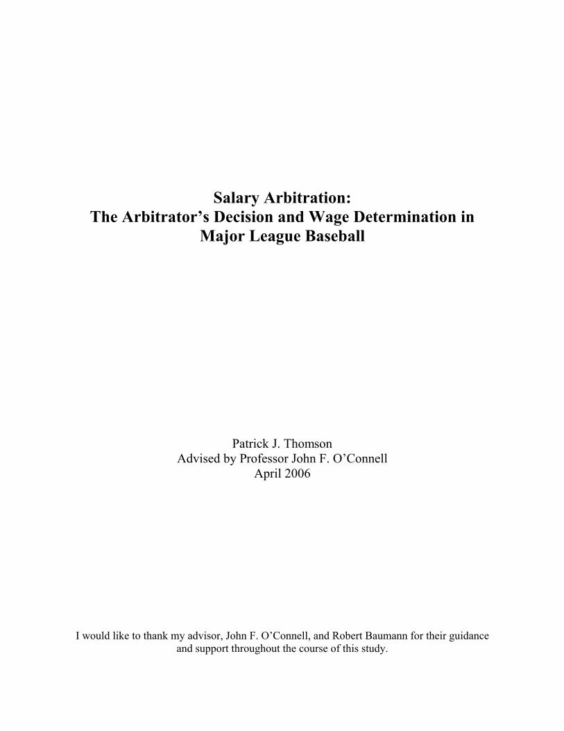
The equation was estimated annually. The coefficients that are derived through the

use of a probit regression may not be interpreted as marginal effects. In order for that

interpretation to be viable, further statistical work is required. The raw coefficients resulting

from a probit regression may be interpreted for their sign and significance.

Ashenfelter and Bloom (1984) show that from the coefficients in the probit model, one

can derive estimates of the mean (µp) and the standard deviation (σp) of the arbitrator’s notion

of a fair award. Ashenfelter and Bloom (1984) were able to verify that the coefficients served

as accurate estimators because their data set, that of unionized municipal law enforcement and

fire protection employees, included both final-offer arbitration results and conventional

arbitration results. The authors used the conventional arbitration results, where the arbitrator

was able to reach a decision based upon his or her notion of a fair award between the offers of

the two parties, to verify that the coefficients were accurate estimators. The following

equation shows specifically how the coefficients of the regression estimate the mean and

standard deviation of the arbitrator’s notion of a fair award:

P

Peu

P

WWP

2

1(2)

The inverse of the coefficient on the average of the two parties’ offers, β1, serves as an

accurate estimate of the standard deviation of the arbitrator’s notion of a fair award. The ratio

of the coefficients, β2/β1, estimates the mean of the arbitrator’s notion of a fair award.

Thomson 17

Since salary arbitration in baseball began prior to the 1974 season, this study will

include data from all hearings which occurred from the program’s inception through the

hearings that occurred prior to the 2004 season. The data set includes observations on 460

arbitration hearings spanning the thirty-one years of the Major League Baseball program. I

estimated the probit regression with annual subsets of the data set as was done by Ashenfelter

and Bloom (1984) in their modeling. The number of observations by year ranged from 35 in

1986 to 5 each in 1997 and 2002. The model was also estimated with the entire data set. This

regression on the entire data set was conducted twice, first with the nominal figures from all

31 years and then with real figures. In order for the second of these tests to be conducted,

nominal salaries from the 31 years of the salary arbitration system were adjusted to real

figures with a base year of 2000. Annual mean salary data were used to construct a Major

League Baseball wage index.4 This index was then used to prepare real wages for

comparison.

The success or failure of our attempted application of arbitrator decision modeling to

the case of Major League Baseball is best ascertained by comparing our regression results to

those of Ashenfelter and Bloom (1984). They had the luxury of verifying their results by

comparing the coefficients stemming from final-offer arbitration regressions to the recorded

results of conventional arbitration. Unfortunately, the salary arbitration system in Major

League Baseball relies solely on final-offer arbitration, so this paper does not have the same

means of comparison.

Examination of the results reported in Ashenfelter and Bloom (1984) provides an

indication of the sign that should be expected in the probit regression results. Specifically, the

4 Mean salary data collected by ESPN, reported by Rodney Fort.

Thomson 18

regression results reported by Ashenfelter and Bloom (1984) all contained a positive sign on

both the regression coefficient and the constant. Our regression coefficients are found in

Table 3 attached. The regression results do not boast the same uniformity of sign. In

addition, a number of the estimators calculated from the regression coefficients are not

reasonable estimates of the mean and standard deviation. For example, the estimated mean

arbitrated wage in 1991 based upon the calculations of this study was approximately four

million dollars. During 1991, the actual mean arbitrated salary throughout all of Major

League Baseball was only $891,188. When the regression was estimated with the entire data

set, the results succeeded in showing the uniformity of sign reported by Ashenfelter and

Bloom (1984). This uniformity of sign was present when the test was conducted with both

nominal and real figures. Estimating the regression once for the entire data set may introduce

changes in the climate surrounding the arbitration proceedings. These changes, if they exist,

are not controlled for in the model and may, therefore, alter the regression results.

There is yet another manner in which the results obtained from the Ashenfelter and

Bloom (1984) model may be examined. I compare the mean of the predicted awards to the

mean of the actual awards. The mean of the actual awards, reported in real terms, is $800.50

with a standard deviation of $1,204.59. The predicted mean of the predicted awards is

$4,034.53 with a standard deviation of $27,624.31. These results would suggest that the

model does not accurately predict the real awards. In addition, the McFadden R2 was very

small and the coefficients were statistically insignificant using the usual level of significance.

Wage Determination

The wage that is determined by final-offer salary arbitration will be examined in order

to show how well it is explained by a number of factors, both those that the arbitrator is and is

Thomson 19

not instructed to take into account. The dependent variable will be the natural log of the

wage. Use of the natural log of the wage is convenient because coefficients on the regressors

may be interpreted as indicating a percentage change in the wage. Nominal wages awarded

by the arbitrator were all adjusted for inflation using the Bureau of Labor Statistics Consumer

Price Index for All Urban Consumers reported in year 2000 nominal dollars.

The variables used were those common to wage determination functions. The variable

Career Length is measured as the number of seasons in which the player has recorded

experience at the Major League level, measured in whole years. The variables Career

Performance and Previous Performance are measured as the number of “win-shares”

attributed to a player over his entire career and in the previous season. The win share is a

relatively new baseball statistic developed by Bill James, renowned as one of the forefathers

of the study of baseball statistics, known as sabermetrics. By definition, each game that a

team wins allows for the allocation of three win shares to the team’s players. A win share is a

single number assigned to a player to represent his contributions to his team’s wins. Bill

James’ win share is adjusted for variables such as ballpark, league, and era. The statistic is

useful because it allows for the comparison across different time periods and different

positions on the baseball field. The variable Team Performance is the winning percentage of

the team involved in the proceedings in the previous season. The variable Previous

Compensation is the player’s salary in the previous season, adjusted for inflation using the

Bureau of Labor Statistics’ Consumer Price Index for All Urban Consumers and reported in

year 2000 nominal dollars. The variable Age of the Stadium is the number of seasons that

have passed since the stadium first officially opened. The variable for the presence of a New

Stadium is binary, which takes a value of one if the stadium was built since 1992 and a value

Thomson 20

of zero if the stadium was constructed prior to 1992. New stadia are typically able to take

advantage of more and varied revenue streams stemming from concession and souvenir sales,

as well as parking and luxury suites, than their predecessors which were built solely to hold

spectators. The variable Metropolitan Population is the number of people residing in the

metropolitan region as reported by the United States Census Bureau. Observations with

players from the clubs in Canada, both in Montreal and Toronto, were excluded. The

variables which address a player’s fielding position are binary, which take a value of one if

the player plays that position and a value of zero if the player does not play the position being

addressed. The position of designated hitter will serve as the basic case, against which the

effects of all other positions will be compared. The variables which address the various

Collective Bargaining Agreements under which salary arbitration has occurred are binary

variables. These variables take on a value of one if the arbitration proceeding occurred under

the auspices of that agreement and a value of zero if the arbitration proceeding did not occur

under the labor agreement being addressed. This first agreement, which covered arbitration

proceedings which occurred prior to the 1974 through 1976 seasons, represents the excluded

case, against which the effects of future agreements will be compared. Finally, a time series

was included, where the year 1974 took on a value of 1, then the index increased by one as

each year progressed. This variable was included to account for the growth in real salaries

over the time period. The Consumer Price Index was utilized to account for inflation, but

salaries in professional baseball have risen at a pace above and beyond that of nation-wide

inflation. Since 1988, the CPI has increased at an average annual rate of 3.0 percent.5 Over

5 Data regarding the Consumer Price Index is compiled and released by the United States Department of Labor, Bureau of Labor Statistics.

Thomson 21

the same time period, mean salaries in Major League Baseball have increased at an average

annual rate of 12.7 percent.6

The regression results for various models may be found in Table 4. The first of these

regressions focuses on four characteristics of the player (Career Length, Career Performance,

Previous Performance, and Previous Compensation) and on four characteristics of the team

(Team Performance, Age of Stadium, New Stadium, and Metropolitan Population). In

addition, the time-variable was included. This will be considered the basic regression form,

as all of these variables will be included in each of the three following regressions. The

coefficients on the variables for Career Length, Career Performance, Previous Performance,

Previous Compensation, and New Stadium are statistically significant at the 99-percent

confidence level. In addition, the time-variable is significant at the 99-percent confidence

level.

The second regression includes the variables from the basic regression, as well as

binary variables for defensive positions on the baseball field. In this regression, the

coefficients on the variables for Career Length, Career Performance, Previous Performance,

Previous Compensation, and New Stadium are again statistically significant at the 99-percent

confidence level. The time-variable is also significant at the 99-percent confidence level.

None of the coefficients on the binary variables for defensive positions are significant at any

conventional level of confidence. The second regression led to little change in explanatory

power over the first regression, as measured by R2.

The third regression includes the variables from the basic regression, as well as binary

variables for the various Collective Bargaining Agreements that have governed interactions

6 Salary figures in Major League Baseball were compiled and presented by Professor Rodney Fort of Washington State University.

Thomson 22

between labor and management throughout the life of the salary arbitration program. In this

regression, the coefficients on the variables for Career Length, Career Performance, Previous

Performance, and Previous Compensation are again statistically significant at the 99-percent

confidence level. The time-variable is also significant at the 99-percent confidence level.

The coefficients on the binary variables for the Collective Bargaining Agreements that were

active from 1977 through 1981, from 1982 through 1985, from 1986 through 1990, and from

1991 through 1995 were statistically significant at the 99-percent confidence level. In

addition, the coefficient on the binary variable for the Collective Bargaining Agreement that

was active from 1996 through 2001 was significant at the 95-percent confidence level. The

third regression led to some notable gain in explanatory power over the previous two

regressions, as measured by R2.

The fourth and final regression includes all of the variables that were previously

mentioned, including those in the basic regression, as well as binary variables representing

defensive positions and binary variables representing Collective Bargaining Agreements. In

this regression, the coefficients on the variables for Career Length, Career Performance,

Previous Performance, and Previous Compensation are again statistically significant at the 99-

percent confidence level. The time-variable is also significant at the 99-percent confidence

level. Finally, the coefficients on the binary variables for the Collective Bargaining

Agreements that were active from 1977 through 1981, from 1982 through 1985, from 1986

through 1990, and from 1991 through 1995 were again statistically significant at the 99-

percent confidence level. In addition, the coefficient on the binary variable for the Collective

Bargaining Agreement that was active from 1996 through 2001 was significant at the 95-

Thomson 23

percent confidence level. The fourth regression led to some gain in explanatory power over

the previous three regressions, as measured by R2.

The sign of the coefficient on the significant variables in each of the regressions

indicate whether the variable has a positive or negative effect on the arbitrated wage. These

true signs may be compared to our intuition as to the effect of each variable. Throughout all

four regressions, the sign on two of the coefficients of variables measuring the player’s career

proved to be as expected. Specifically, as a player’s previous salary increases, so too does the

wage. In the first two regressions, the sign on the coefficient of the variable measuring a

player’s career length is negative, while in the later two regressions, the sign on this same

variable is positive. The negative sign indicates that as a career is lengthened, the arbitrated

wage falls. This could be caused by the belief that there exist diminishing returns throughout

the career of a baseball player. On the other hand, the positive sign indicates that as a career

is lengthened, the arbitrated wage rises. This could be caused by some seniority effect that

becomes more pronounced as the length of a career increases. The sign on the coefficient of

the New Stadium variable had a sign opposite of that which was expected. When a new

stadium is present and there are presumably higher revenue streams available to the employer,

one would expect the predicted wage to rise.

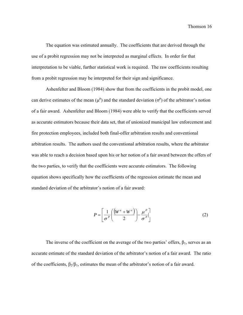
In the later two regressions, the sign on the variables for each of the Collective

Bargaining Agreements signifies an increase in the predicted wage over that in the excluded

case of the Collective Bargaining Agreement in effect from 1794 through 1976. Perhaps a

more telling test is how the coefficient on each Collective Bargaining Agreement compares to

that of the previous Agreement. In order to examine this relationship, F-tests were conducted

on the coefficients of the various Collective Bargaining Agreement variables. Results from

Thomson 24

the F-tests are included in Table 5. There is a significant and positive effect on wage between

the first Agreement of 1974 and the second Agreement of 1977. This significance may be

interpreted from the coefficient on the variable for the 1977 Agreement in the third and fourth

regressions. There is a significant difference between the Collective Bargaining Agreement

of 1991 and the Agreement of 1996. The difference between these two Agreements has a

negative effect on wages. There is also a significant difference between the Collective

Bargaining Agreement of 1996 and the Agreement of 2002. The difference between these

two Agreements has a negative effect of wages. This test does not find a significant

difference between the Agreements of 1977 and 1982, the Agreements of 1982 and 1986, or

the Agreements of 1986 and 1991.

The estimated wage functions explain a good deal of the variation in the wage. The

most basic regression has an adjusted R2 value of 0.885, and the most elaborate regression has

an adjusted R2 value of 0.950.

Following the individual examination of the two stages described in this paper, the

two may be studied together, with a goal of estimating the player’s market wage and

predicting the arbitrator’s decision. I will use the estimated wage function to predict a market

wage for each player whose case proceeds through salary arbitration. That market salary

estimate will be considered the arbitrator’s notion of a “fair award.” This notion of a fair

award, along with the wage offers of the club and the player, will be incorporated into the

basic model used by Ashenfelter and Bloom. Use of this basic model will allow me to predict

the arbitrator’s decision by observing which of the offers of the two parties is closer to the

estimated arbitrator’s notion of a fair award.

Thomson 25

When the theory from the two separate tests in this paper was incorporated together, a

market wage was individually estimated for each player whose case went through the

arbitration process. This estimated wage, used to represent the arbitrator’s notion of a fair

award, was then used in concert with the wage offers of the two parties to predict the

arbitrator’s decision in each case. These predicted decisions were compared to the known

decisions in each case to determine how well this process modeled the actual arbitration

process. This paper’s modeling was able to correctly predict the arbitrator’s decision

approximately 54-percent of the time.

VII. Summary and Conclusions

Baseball is but one of many cases in which arbitration is used to settle negotiating

disputes. With so much riding upon the outcome of these proceedings, there is much to be

gained from the strategic implications that would come with accurate modeling of the

arbitration proceeding. The importance of accurate modeling led me to examine a number of

established modeling techniques as they apply to the case of Major League Baseball.

The basic modeling of the arbitrator’s decision by Ashenfelter and Bloom has been

shown not to work in this case. When the probit regression is estimated annually, the

coefficients do not always take the expected sign, and a number of the coefficients do not

present reasonable estimates of the mean and standard deviation of the arbitrator’s notion of a

fair award, as was suggested in the theory. The coefficients do take the expected sign when

the probit regression is estimated over the entire population. Unfortunately, the coefficients

are not reasonable estimates of the mean and standard deviation of the arbitrator’s notion of a

fair award in the case of the entire population. While it is evident that the modeling of the

Thomson 26

arbitrator’s decision may not be applied in this case, the reasons for the model’s lack of fit are

less clear. This paper suggests that a number of characteristics of the labor market in Major

League Baseball are different from those of the labor market in which the model was first

constructed. First, there is a great deal of variation in the salaries commanded by baseball

players, ranging from the league minimum ($300,000 in 2004) to annual salaries numbering

tens of millions of dollars. Variation was not present to the same extent in the salaries for

municipal police and fire employees, the labor market first modeled by Ashenfelter and

Bloom. Second, there is no typical productivity of a professional baseball player. The

production statistics of a baseball player vary widely from the superstar to the journeymen

filling out a roster. Skill differentiation was not as pronounced in the case of municipal police

and fire employees.

Modeling a wage function based upon a number of market variables suggests that the

final arbitrator’s award is quite similar to a market determined wage. This would suggest that,

ignoring costs associated with the arbitration process, final offer arbitration is a relatively

effective substitute for a strictly market determined wage. Of course, the apparent precision

of the final arbitrator’s award is reflection of the two parties to the dispute, as the arbitrator is

forced to make a selection of one of the two offers.

One of the motivations behind this research is the interest that both parties to an

arbitration dispute have in properly modeling the proceeding. When the entire arbitration

proceeding is modeled, from wage determination through arbitrator decision, this paper’s

modeling correctly predicts the decision approximately 54-percent of the time. This paper

makes a step in the direction of modeling the arbitration process, but more work remains to be

Thomson 27

done. Specifically, more precise wage functions or better models of the arbitrator’s decision

would increase the effectiveness of this modeling.

Major League Baseball salary arbitration is an event with increasingly high stakes

where there is always one winner and one loser. Much of the modeling discussed in this

paper was first designed and introduced to study other occupations. Any advances made in

this modeling could quite effectively be applied to other industries with salary arbitration.

Thomson 28

Table 1: History of Arbitration Filings and Hearings

YearCases Filed

Cases Heard

% Heard

1974 53 29 54.7%1975 38 16 42.1%1976 0 0 N/A1977 0 0 N/A1978 16 9 56.3%1979 40 12 30.0%1980 65 26 40.0%1981 96 21 21.9%1982 103 23 22.3%1983 88 30 34.1%1984 80 10 12.5%1985 98 13 13.3%1986 159 35 22.0%1987 109 26 23.9%1988 111 18 16.2%1989 136 12 8.8%1990 162 24 14.8%1991 157 17 10.8%1992 147 20 13.6%1993 118 18 15.3%1994 80 16 20.0%1995 61 8 13.1%1996 76 10 13.2%1997 80 5 6.3%1998 81 8 9.9%1999 62 11 17.7%2000 90 10 11.1%2001 102 14 13.7%2002 93 5 5.4%2003 72 7 9.7%2004 75 7 9.3%

Thomson 29

Table 2: Historical Results of Arbitration Proceedings

YearCases Heard

Player Victory

Team Victory

% Team Victory

1974 29 13 16 55.2%

1975 16 6 10 62.5%

1976 01977 01978 9 2 7 77.8%

1979 12 8 4 33.3%

1980 26 15 11 42.3%

1981 21 11 10 47.6%

1982 23 8 15 65.2%

1983 30 13 17 56.7%

1984 10 4 6 60.0%

1985 13 6 7 53.8%

1986 35 15 20 57.1%

1987 26 10 16 61.5%

1988 18 7 11 61.1%

1989 12 7 5 41.7%

1990 24 14 10 41.7%

1991 17 6 11 64.7%

1992 20 9 11 55.0%

1993 18 6 12 66.7%

1994 16 6 10 62.5%

1995 8 2 6 75.0%

1996 10 7 3 30.0%

1997 5 1 4 80.0%

1998 8 3 5 62.5%

1999 11 2 9 81.8%

2000 10 4 6 60.0%

2001 14 6 8 57.1%

2002 5 1 4 80.0%

2003 7 2 5 71.4%

2004 7 3 4 57.1%

Thomson 30

Table 3: Decision Modeling Results

n Year β 2 β1 McFadden R2σ μ

29 1974 0.59702 (0.56355) -0.00882 (0.00974) 0.02130 -113.423 -67.7154

16 1975 -0.35349 (0.74861) 0.00967 (0.01001) 0.04785 103.3788 -36.5435

0 1976

0 1977

9 1978 -0.03594 (1.51290) 0.01119 (0.02078) 0.03474 89.34922 -3.21118

12 1979 -1.43893 (1.17630) 0.01558 (0.01709) 0.05579 64.20399 -92.385

26 1980 0.89391 (0.92102) -0.00894 (0.00758) 0.07199 -111.891 -100.021

21 1981 0.17989 (0.57214) -0.00108 (0.00228) 0.00786 -923.774 -166.177

23 1982 -0.10633 (0.64322) 0.00162 (0.00192) 0.02446 618.1531 -65.7255

30 1983 0.13515 (0.50982) 0.00009 (0.00132) 0.00013 10559.78 1427.197

10 1984 -7.69628 (0.07558) 0.02171 (0.00005) 0.00082 46.06584 -354.536

13 1985 0.05493 (0.64846) 0.00008 (0.00108) 0.00032 12182.42 669.1845

35 1986 0.13360 (0.44849) 0.00009 (0.00080) 0.00029 10592.94 1415.196

26 1987 1.41870 (0.70244) -0.00169 (0.00102) 0.11326 -592.914 -841.165

18 1988 -0.41266 (0.68332) 0.00107 (0.00099) 0.06199 933.6505 -385.276

12 1989 0.97938 (1.12835) -0.00168 (0.00153) 0.08630 -596.736 -584.432

24 1990 -1.35394 (0.66924) 0.00125 (0.00066) 0.12176 798.0911 -1080.57

17 1991 0.28006 (0.63874) 0.00007 (0.00039) 0.00138 14671.37 4108.861

20 1992 0.84948 (0.53149) -0.00044 (0.00028) 0.10305 -2256.25 -1916.65

18 1993 0.72335 (0.61867) -0.00016 (0.00029) 0.01320 -6257.79 -4526.58

16 1994 0.37807 (0.54331) -0.00003 (0.00021) 0.00087 -35823.8 -13544.1

8 1995 1.12878 (1.08296) -0.00019 (0.00039) 0.02601 -5232.88 -5906.76

10 1996 -0.20159 (0.71454) -0.00015 (0.00027) 0.02544 -6637.47 1338.065

5 1997 3.24939 (3.29073) -0.00138 (0.00167) 0.21099 -727.066 -2362.52

8 1998 2.27063 (1.33709) -0.00163 (0.00127) 0.48434 -612.659 -1391.12

11 1999 4.17550 (2.77638) -0.00102 (0.00075) 0.34054 -985.19 -4113.66

10 2000 -0.48510 (0.65155) 0.00040 (0.00034) 0.19367 2504.225 -1214.81

14 2001 0.55018 (0.66997) -0.00015 (0.00023) 0.02237 -6788.58 -3734.97

5 2002

7 2003 0.79324 (0.97844) -0.00006 (0.00021) 0.00904 -17114.7 -13576.1

7 2004 -0.23600 (0.90367) 0.00017 (0.00033) 0.03212 5752.01 -1357.47

460 All YearsReal 0.14625 (0.07099) 0.0000421 (0.00005) 0.00120 23752.97 3473.872

Nominal 0.14605 (0.07465) 0.0000362 (0.00005) 0.00091 27624.31 4034.53

* Figures for σ andµ are recorded in thousands of dollars.(Standard Errors in Parenthesis)

Thomson 31

Table 4: Wage Determination Regression Results

Regression 1 2 3 4

Constant 2.227549*** 2.330127*** 1.250610*** 1.119554***(0.235493) (0.350954) (0.194108) (0.293746)

Career Length -0.003089*** -0.003739*** 0.002414*** 0.001934**(0.001001) (0.001077) (0.000759) (0.000869)

Career Performance 0.003286*** 0.003558*** 0.004428*** 0.004596***(0.000919) (0.000926) (0.000609) (0.000694)

Previous Performance 0.048102*** 0.053304*** 0.041878*** 0.047706***(0.004689) (0.004907) (0.003420) (0.003543)

Team Performance -0.212436 -0.423571 0.524733 0.298181(0.473163) (0.463120) (0.353341) (0.341588)

Previous Compensation 0.000391*** 0.000374*** 0.000416*** 0.000398***(0.000063) (0.000061) (0.000038) (0.000037)

Time Variable 0.177638*** 0.175981*** 0.154699*** 0.151026***(0.004928) (0.006344) (0.016581) (0.016063)

Position 1B -0.078111 0.115498(0.293507) (0.247914)

Position 2B -0.234258 -0.023804(0.291369) (0.248482)

Position 3B -0.252028 -0.003852(0.213825) (0.246534)

Position C -0.080215 0.151397(0.297755) (0.259148)

Position OF -0.213583 0.070686(0.286163) (0.242224)

Position P 0.108796 0.359573(0.284283) (0.241978)

Position SS -0.276457 0.179214(0.306249) (0.255233)

CBA 2 1.018669*** 0.986674***(0.236717) (0.194434)

CBA 3 1.256218*** 1.23399***(0.175029) (0.171100)

CBA 4 1.231764*** 1.241598***(0.233001) (0.225439)

CBA 5 1.329387*** 1.376053***(0.317397) (0.311655)

CBA 6 0.808186* 0.858899**(0.419910) (0.410726)

CBA 7 0.431402 0.415086(0.484997) (0.470297)

Age of Stadium 0.887975 0.001393 0.001096 0.001346(0.001391) (0.001310) (0.001033)

New Stadium -0.496438*** -0.474458*** -0.076329 -0.051848(0.145192) (0.143005) (0.106949)

Metropolitan Population 0.00000015 0.00000016 -0.000000004 -0.000000004(0.000000013) (0.000000012) (0.000000009)

R^2 0.887975 0.896275 0.946105 0.953532Adjusted R^2 0.884956 0.891185 0.943641 0.950337

(White Heteroskedasticity Standard Errors in Parenthesis)* 90 -Percent Confidence Level** 95 -Percent Confidence Level*** 99 -Percent Confidence Level

Thomson 32

Table 5: F-Test Statistics for Collective Bargaining Agreement Variables

Hypothesis F-Stat Prob Conclusion

CBA 2 = CBA 3 1.918258 0.167014 CBA 2 = CBA 3CBA 3 = CBA 4 0.007888 0.929285 CBA 3 = CBA 4CBA 4 = CBA 5 1.633972 0.202081 CBA 4 = CBA 5CBA 5 = CBA 6 14.89807 0.000137 CBA 5 ≠ CBA 6CBA 6 = CBA 7 15.31319 0.000111 CBA 6 ≠ CBA 7

Thomson 33

Figure 1

History of Arbitration Filings and Hearings

R2 = 0.6253

0

0.1

0.2

0.3

0.4

0.5

0.6

1970 1975 1980 1985 1990 1995 2000 2005

Year

Pe

rce

nta

ge

of

Cas

es

Hea

rd

Figure 2

Thomson 34

Historical Results of Arbitration Proceedings

R2 = 0.1012

0

0.1

0.2

0.3

0.4

0.5

0.6

0.7

0.8

0.9

1970 1975 1980 1985 1990 1995 2000 2005

Year

Per

cen

tag

e o

f C

ases

Wo

n B

y T

eam

Thomson 35

Bibliography

Ashenfelter, Orley (1987). “Arbitrator Behavior.” The American Economic Review, 77(2)

(May): 342-346.

Ashenfelter, Orley and David E. Bloom (1984). “Models of Arbitrator Behavior: Theory and

Evidence.” The American Economic Review, 74(1) (March): 111-124.

Ashenfelter, Orley and Gordon B. Dahl (2005). “Strategic Bargaining Behavior, Self-Serving

Biases, and the Role of Expert Agents: An Empirical Study of Final-Offer

Arbitration.” National Bureau of Economic Research Working Papers, 11189.

Burger, John D. and Stephen J.K. Walters (2005). “Arbitrator Bias and Self-Interest” Lessons

from the Baseball Labor Market.” Journal of Labor Research, 26(2) (Spring): 267-

280.

Burgess, Paul L. and Daniel R. Marburger (1993). “Do Negotiated and Arbitrated Salaries

Differ Under Final-Offer Arbitration?.” Industrial and Labor Relations Review, 46(3)

(April): 548-559.

Crawford, Vincent (1979). “On Compulsory-Arbitration Schemes.” Journal of Political

Economy, 87 (February): 131-160.

Faurot, David J. and Stephen McAllister (1992). “Salary Arbitration and Pre-Arbitration

Negotiation in Major League Baseball.” Industrial and Labor Relations Review, 45(4)

(July): 697-710.

Fizel, John (1994). “Play Ball! Baseball Arbitration at 20.” Dispute Resolution Journal, 49()

(June): 42-47.

Fizel, John (1996). “Bias in Salary Arbitration: The Case of Major League Baseball.” Applied

Economics, 28(2) (February): 255-265.

Thomson 36

Fizel, John, Anthony C. Krautmann, and Lawrence Hadley (2002). “Equity and Arbitration in

Major League Baseball.” Managerial and Decision Economics, 23 (7)

(October/November): 427-35.

Frederick, David M., William H. Kaempfer, and Richard L. Wobbekind (1992). “Salary

Arbitration as a Market Substitute.” Paul M. Sommers, ed. Diamonds Are Forever:

The Business of Baseball, Washington, D.C.: Brookings Institute: 29-49.

Guis, Mark P. and Timothy R. Hylan (1999). “Testing for the Effect of Arbitration on the

Salaries of Hitters in Major League Baseball: Evidence from Panel Data.”

Pennsylvania Economic Review, 7(1) (Spring): 28-35.

Malburger, Daniel R. (2004). “Arbitrator Compromise in Final Offer Arbitration: Evidence

from Major League Baseball.” Economic Inquiry, 42(1) (January): 60-68.

Marburger, Daniel R. and John F. Scoggins (1996). “Risk and Final Offer Arbitration Usage

Rates: Evidence from Major League Baseball.” Journal of Labor Research, 17(4)

(Fall): 735-745.

Scully, Gerald W. (1974). “Pay and Performance in Major League Baseball.” The American

Economic Review, 64(6) (December): 915-930.

Scully, Gerald W. (1978). “Binding Salary Arbitration in Major League Baseball.” American

Behaviorial Scientist, 21() (): 431-450.

Scully, Gerald W. (1999). “Free Agency and the Rate of Monopsonistic Exploitation in

Baseball.” Competition Policy in Professional Sports: Europe After the Bosman Case:

59-69.

Stevens, Carl M. (1996). “Is Compulsory Arbitration Compatible With Bargaining?”

Industrial Relations, 5 (February): 38-52.