A New DA and TM Based Approach to Design Air-Core Magnets

Shashikant Manikonda

Taylor Model Methods VII, Dec 14th-17th, 2011, Key West, Florida

2

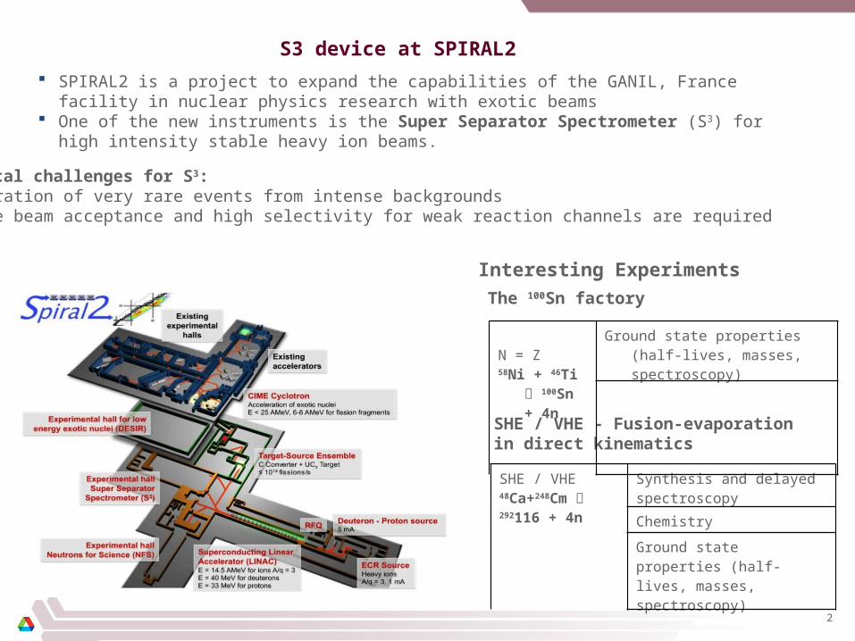
S3 device at SPIRAL2

SHE / VHE - Fusion-evaporation in direct kinematics

SHE / VHE48Ca+248Cm 292116 + 4n

Synthesis and delayed spectroscopy

Chemistry

Ground state properties (half-lives, masses, spectroscopy)

The 100Sn factory

N = Z58Ni + 46Ti

100Sn + 4n

Ground state properties (half-lives, masses, spectroscopy)

Technical challenges for S3: Separation of very rare events from intense backgrounds Large beam acceptance and high selectivity for weak reaction channels are required

Interesting Experiments

SPIRAL2 is a project to expand the capabilities of the GANIL, France facility in nuclear physics research with exotic beams

One of the new instruments is the Super Separator Spectrometer (S3) for high intensity stable heavy ion beams.

3

MAMS Layout for S3

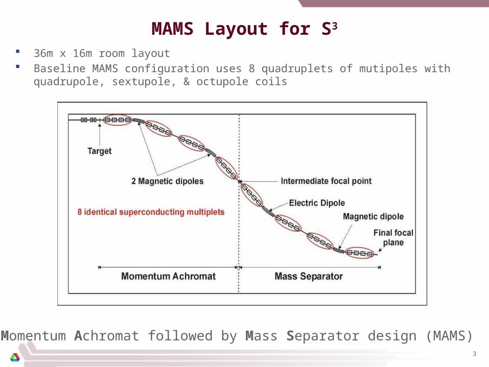
36m x 16m room layout Baseline MAMS configuration uses 8 quadruplets of mutipoles with quadrupole, sextupole, & octupole

coils

Momentum Achromat followed by Mass Separator design (MAMS)

S3 Device Description

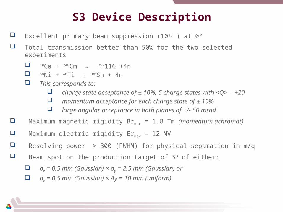
Excellent primary beam suppression (1013 ) at 0°

Total transmission better than 50% for the two selected experiments

48Ca + 248Cm → 292116 +4n 58Ni + 48Ti → 100Sn + 4n This corresponds to:

charge state acceptance of ± 10%, 5 charge states with <Q> = +20 momentum acceptance for each charge state of ± 10% large angular acceptance in both planes of +/- 50 mrad

Maximum magnetic rigidity Brmax = 1.8 Tm (momentum achromat)

Maximum electric rigidity Ermax = 12 MV

Resolving power > 300 (FWHM) for physical separation in m/q

Beam spot on the production target of S3 of either:

σx = 0.5 mm (Gaussian) × σy = 2.5 mm (Gaussian) or

σx = 0.5 mm (Gaussian) × Δy = 10 mm (uniform)

Final focal plane size depending on the experiment

200 x 100 mm (maximum for high resolution mode, e.g. SHE synthesis) 100 x 100 mm (delayed gamma spectroscopy) 50 x 50 mm (low-energy branch gas catcher, GS properties)

Mass Achromat followed by Mass Separator (MAMS) layout choosen for S3

Momentum achromat to suppress primary beam by at least 1:1000. Further beam suppression and mass channel selection by a mass separator stage which is fully achromatic in momentum for each m/q value.

Different operating modes are envisioned for performing experiments

S3 Device Description (Continued)

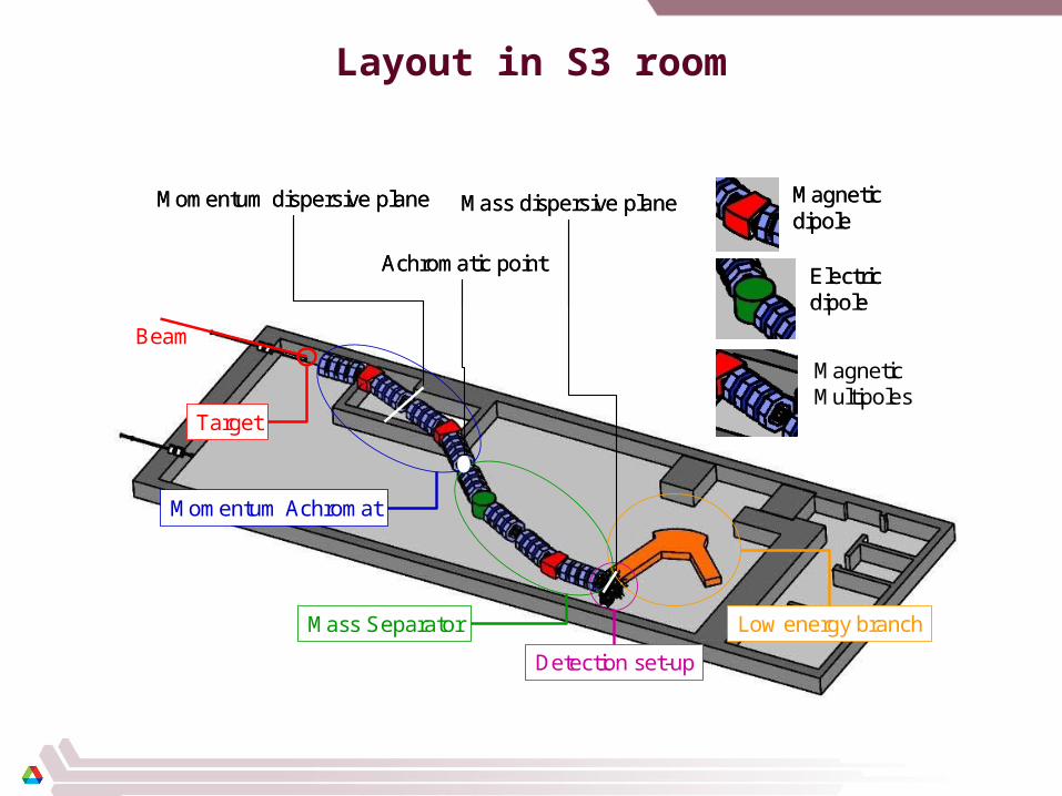
Layout in S3 room

Beam

Target

Momentum Achromat

Mass Separator

Detection set-up

Low energy branch

Momentum dispersive plane

Achromatic point

Mass dispersive plane Magneticdipole

Electricdipole

MagneticMultipoles

Beam

Target

Momentum Achromat

Mass Separator

Detection set-up

Low energy branch

Momentum dispersive plane

Achromatic point

Mass dispersive plane Magneticdipole

Electricdipole

MagneticMultipoles

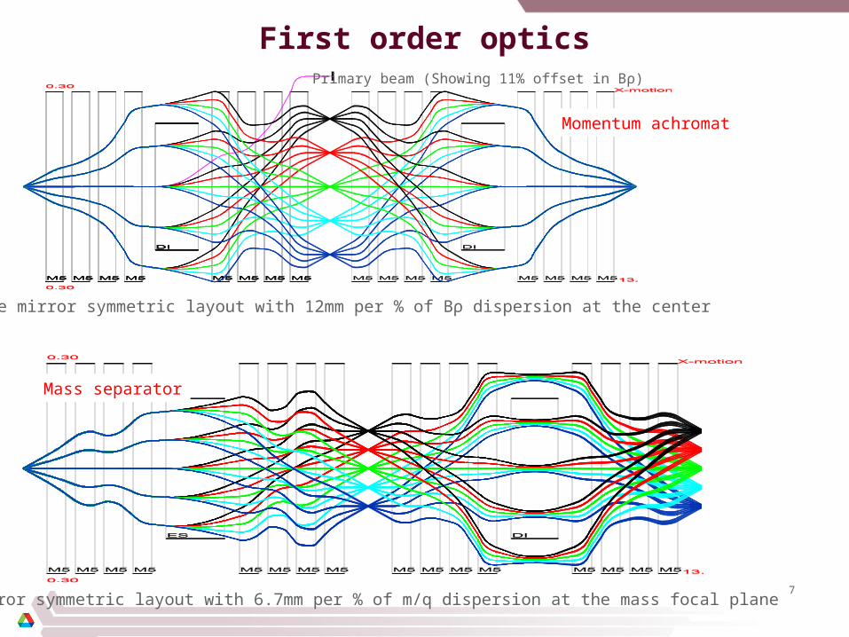
First order optics

7

Primary beam (Showing 11% offset in Bρ)

• Double mirror symmetric layout with 12mm per % of Bρ dispersion at the center

• Mirror symmetric layout with 6.7mm per % of m/q dispersion at the mass focal plane

Momentum achromat

Mass separator

8

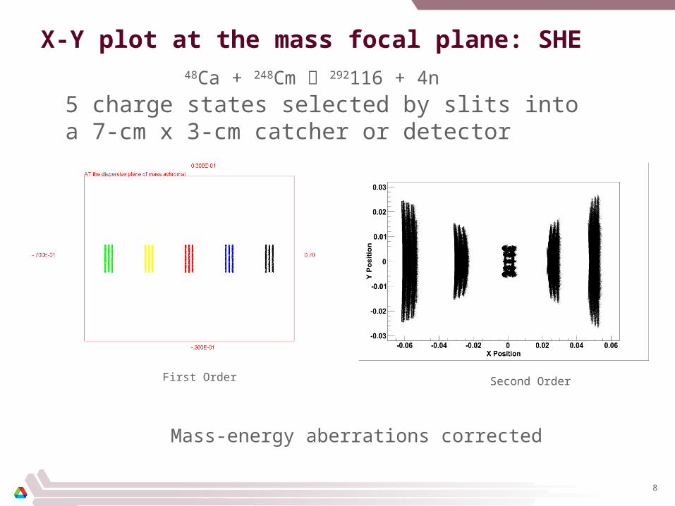
First Order Second Order

X-Y plot at the mass focal plane: SHE

Mass-energy aberrations corrected

5 charge states selected by slits into a 7-cm x 3-cm catcher or detector

48Ca + 248Cm 292116 + 4n

9

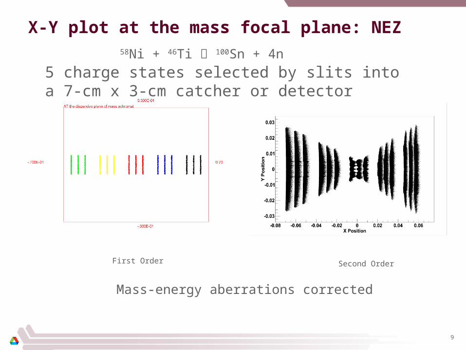
X-Y plot at the mass focal plane: NEZ

First Order Second Order

Mass-energy aberrations corrected

5 charge states selected by slits into a 7-cm x 3-cm catcher or detector

58Ni + 46Ti 100Sn + 4n

10

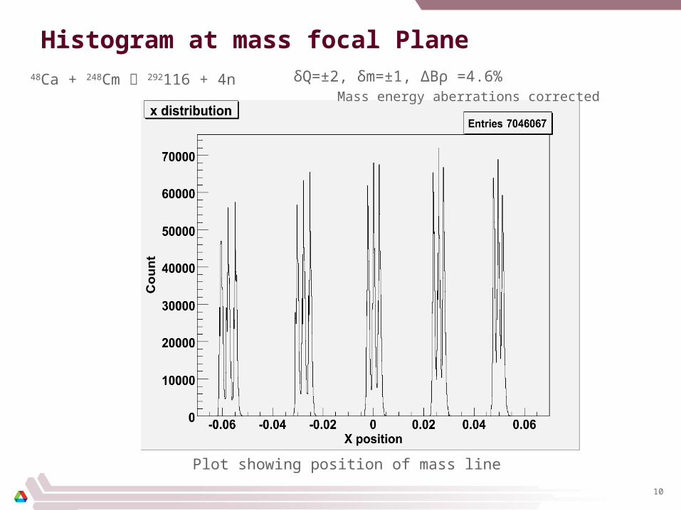
Histogram at mass focal Plane

Plot showing position of mass line

48Ca + 248Cm 292116 + 4n δQ=±2, δm=±1, ∆Bρ =4.6%Mass energy aberrations corrected

11

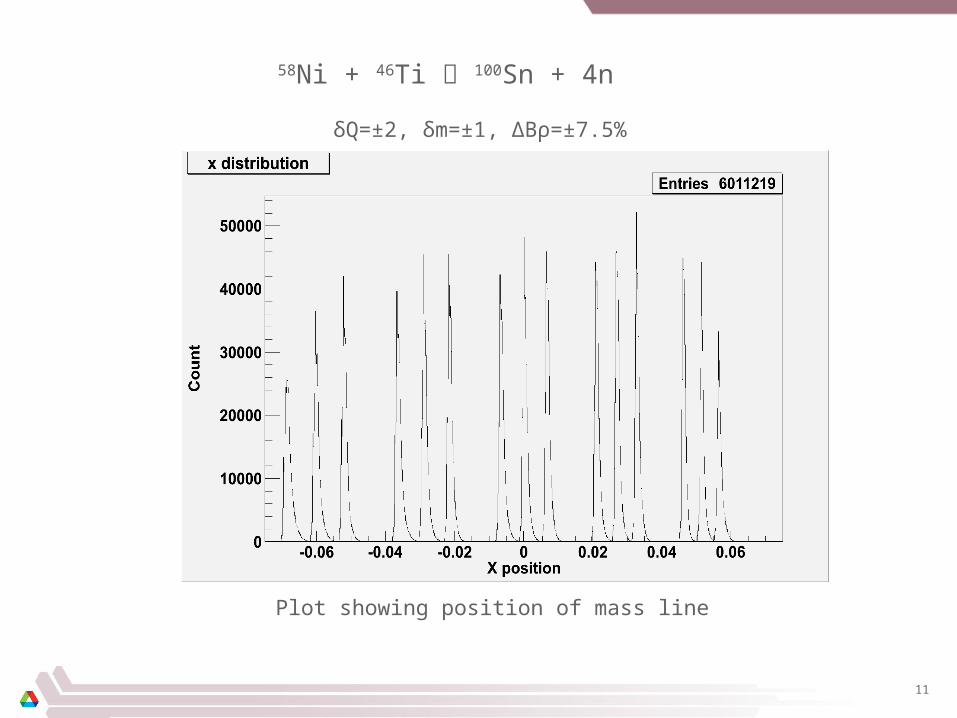
δQ=±2, δm=±1, ∆Bρ=±7.5%

58Ni + 46Ti 100Sn + 4n

Plot showing position of mass line

12

Magnet requirements for S3

8 SC quadruplets or triplets 3 dipoles and 1 electrostatic sector magnet Each singlet has quadrupole, sextupole, & octupole coils, with 30-cm warm bore diameter &

40-cm effective length (octupoles maay not be required) Fields required at 15-cm radius for 2 T-m rigidity (higher rigidity is easy):

– Quadrupole: 1.0 T– Sextupole: 0.3 T– Octupole: 0.3 T

Total power required for cryo-coolers of 8 quadruplets ~160 kW – Warm iron used to speed up cool down (~1 ton per multipole)

Options for Multipole Magnet Design Race track Coils Double Helix Model by AML 3D Cosine theta magnets

13

Type of MagnetsThe electric and magnetic field will depend on the type of magnets we choose.

Some examples: Bending magnets (Dipole) Focusing magnets (Quadrupole) Steering magnets Kicker magnets (thin Quadrupole) Accelerating (Electric element) Corrector magnets ( Hexapole, Octupole etc)

Accelerator lattice consists of array of magnets setup to attain certain goal. Complexity comes from the fact that there are many undetermined parameters. To arrive at a final (fully optimized) beam optic layout requires several iterations between beam optic design studies, magnet design studies and other practical constraints.

14

Magnets for Accelerator Physics Applications

Bρ and Eρ of the beam/recoil– High Energy Physics: Only magnetic elements can be used– Low Energy Nuclear Physics (<10 Mev/nucleon): Both Electric and Magnetic elements

can be used Field quality requirement Operating environment: Radiation Hardened magnets Super conducting or conventional: Depends on field strength requirements Tolerances to errors, misalignments, stress and strain in the support structures,

heating Practical constrains like positioning of beam dumps, detectors, slits, monitors

etc. Other factors: Reuse of existing magnets

Some factors influencing the choice of magnets and the design of magnets

15

During the design phase: – Is the magnet practically feasible to build ?

• Field quality requirement• Cost estimate

– Beam optic properties (Transfer Maps)– Fringe Fields – Misalignment study

After construction – Transfer maps with realistic fields

16

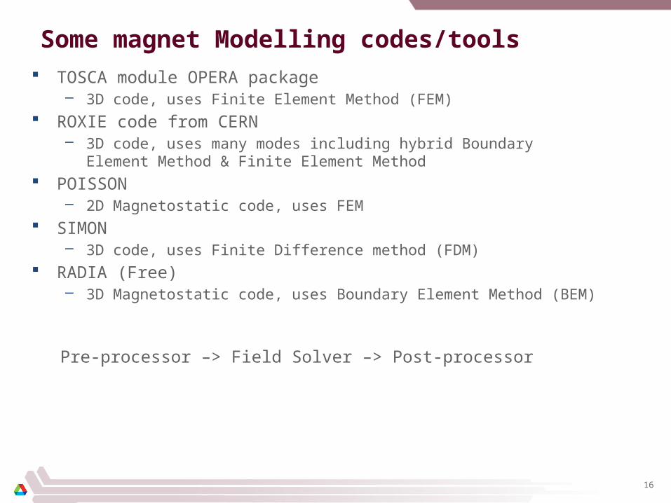
Some magnet Modelling codes/tools TOSCA module OPERA package

– 3D code, uses Finite Element Method (FEM) ROXIE code from CERN

– 3D code, uses many modes including hybrid Boundary Element Method & Finite Element Method

POISSON – 2D Magnetostatic code, uses FEM

SIMON– 3D code, uses Finite Difference method (FDM)

RADIA (Free)– 3D Magnetostatic code, uses Boundary Element Method (BEM)

Pre-processor –> Field Solver –> Post-processor

Magnetic field due to arbitrary current distribution

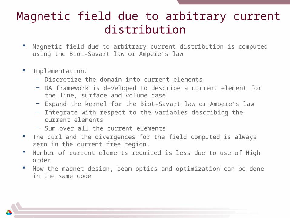
Magnetic field due to arbitrary current distribution is computed using the Biot-Savart law or Ampere’s law

Implementation:– Discretize the domain into current elements– DA framework is developed to describe a current element for the line, surface and

volume case– Expand the kernel for the Biot-Savart law or Ampere’s law– Integrate with respect to the variables describing the current elements– Sum over all the current elements

The curl and the divergences for the field computed is always zero in the current free region.

Number of current elements required is less due to use of High order Now the magnet design, beam optics and optimization can be done in the same code

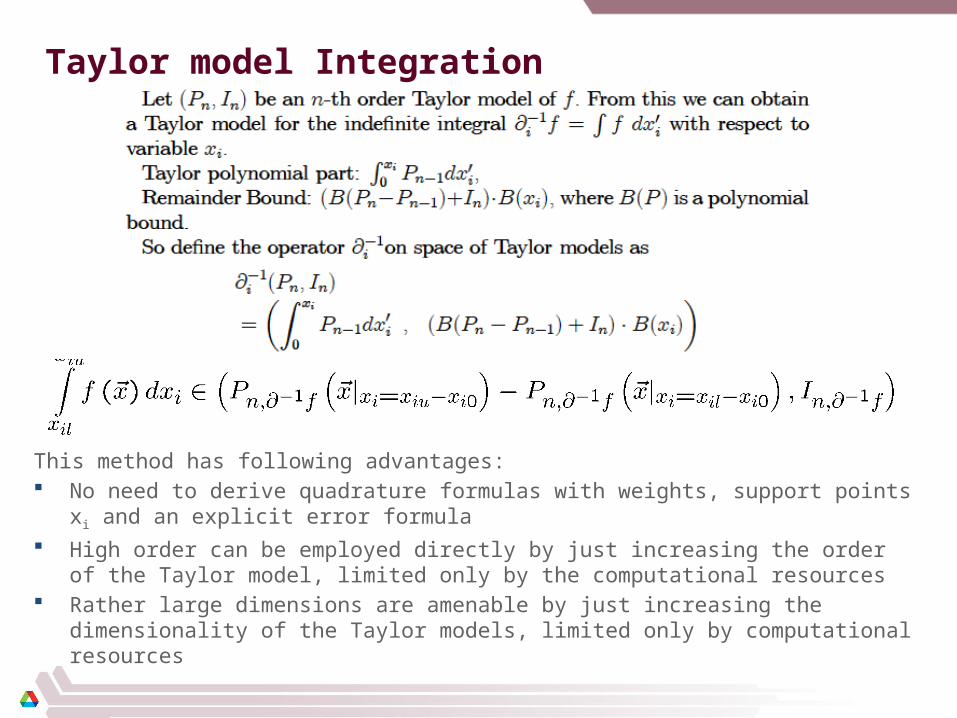
Taylor model Integration

This method has following advantages: No need to derive quadrature formulas with weights, support points x i and an explicit error

formula High order can be employed directly by just increasing the order of the Taylor model, limited only

by the computational resources Rather large dimensions are amenable by just increasing the dimensionality of the Taylor models,

limited only by computational resources

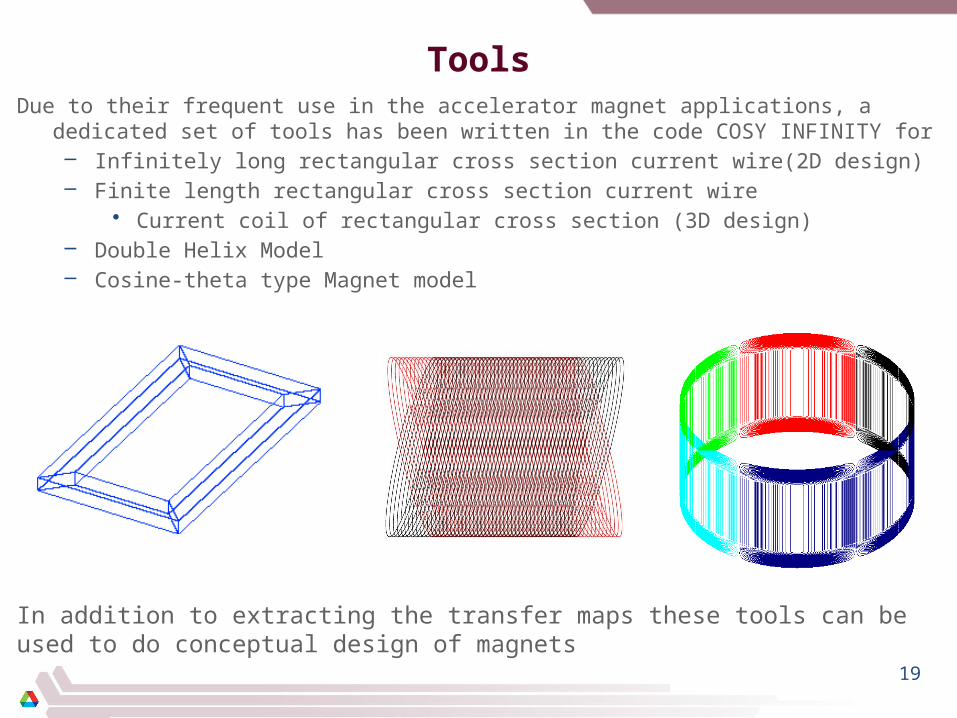
ToolsDue to their frequent use in the accelerator magnet applications, a dedicated set of tools has been written in

the code COSY INFINITY for– Infinitely long rectangular cross section current wire(2D design)– Finite length rectangular cross section current wire

• Current coil of rectangular cross section (3D design)– Double Helix Model– Cosine-theta type Magnet model

In addition to extracting the transfer maps these tools can be used to do conceptual design of magnets

19

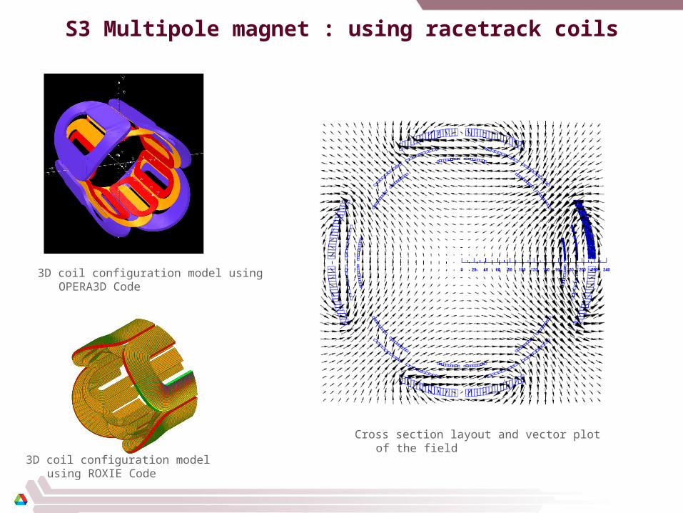
S3 Multipole magnet : using racetrack coils

3D coil configuration model using ROXIE Code

Cross section layout and vector plot of the field

3D coil configuration model using OPERA3D Code

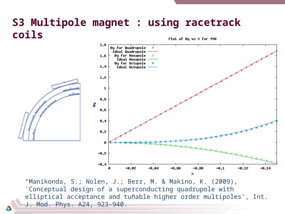
S3 Multipole magnet : using racetrack coils

“Manikonda, S.; Nolen, J.; Berz, M. & Makino, K. (2009), 'Conceptual design of a superconducting quadrupole with elliptical acceptance and tunable higher order multipoles', Int. J. Mod. Phys. A24, 923-940.”

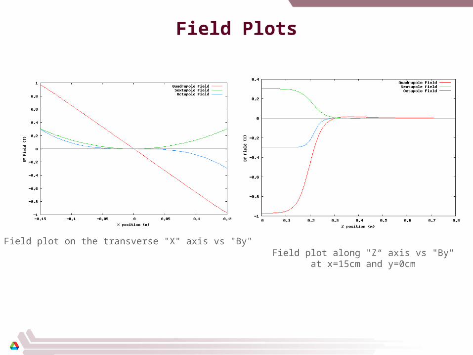
Field Plots

Field plot on the transverse "X" axis vs "By" Field plot along "Z“ axis vs "By" at x=15cm

and y=0cm

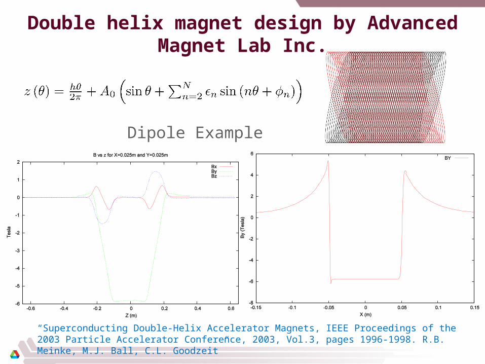
Double helix magnet design by Advanced Magnet Lab Inc.

Dipole Example

“Superconducting Double-Helix Accelerator Magnets, IEEE Proceedings of the 2003 Particle Accelerator Conference, 2003, Vol.3, pages 1996-1998. R.B. Meinke, M.J. Ball, C.L. Goodzeit”

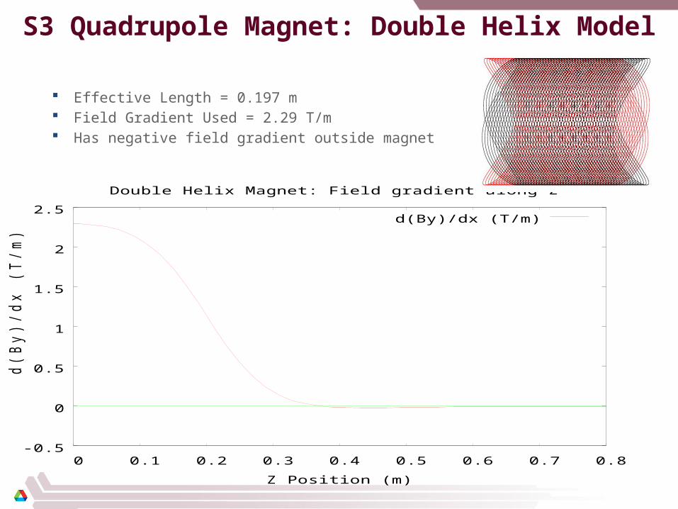
S3 Quadrupole Magnet: Double Helix Model

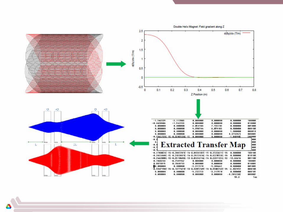
Effective Length = 0.197 m Field Gradient Used = 2.29 T/m Has negative field gradient outside magnet

-0.5

0

0.5

1

1.5

2

2.5

0 0.1 0.2 0.3 0.4 0.5 0.6 0.7 0.8

d(B

y)/

dx (

T/m

)

Z Position (m)

Double Helix Magnet: Field gradient along Z

d(By)/dx (T/m)

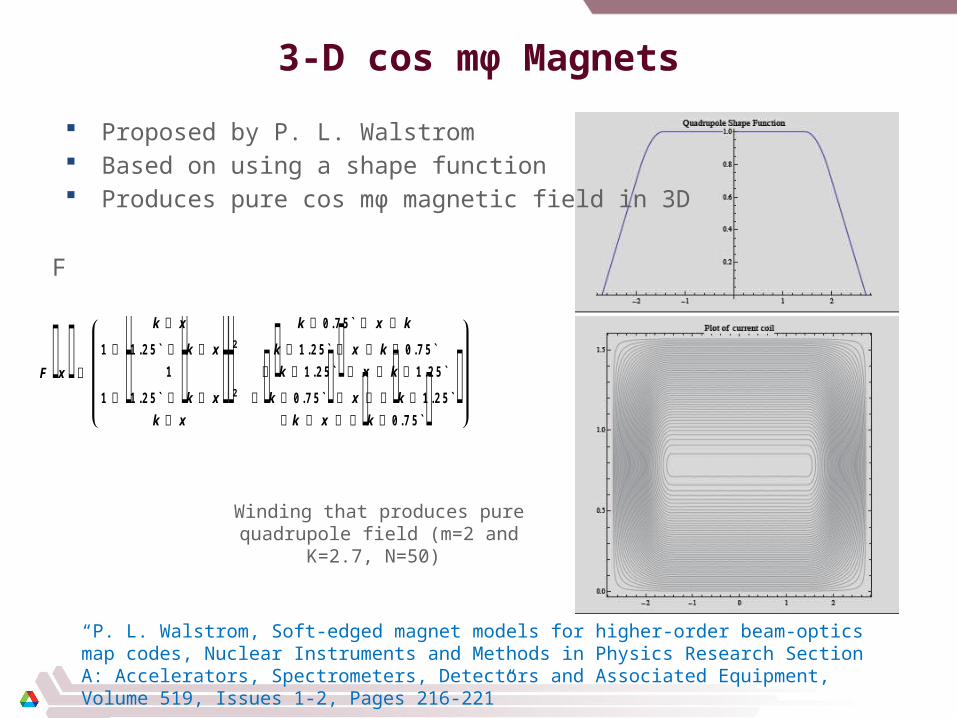
3-D cos mφ Magnets

Proposed by P. L. Walstrom Based on using a shape function Produces pure cos mφ magnetic field in 3D

“P. L. Walstrom, Soft-edged magnet models for higher-order beam-optics map codes, Nuclear Instruments and Methods in Physics Research Section A: Accelerators, Spectrometers, Detectors and Associated Equipment, Volume 519, Issues 1-2, Pages 216-221”

F x

k x k 0 .7 5 ` x k

1 1 .2 5 ` k x 2 k 1 .2 5 ` x k 0 .7 5 `1 k 1 .2 5 ` x k 1 .2 5 `

1 1 .2 5 ` k x 2 k 0 .7 5 ` x k 1 .2 5 ` k x k x k 0 .7 5 `

F

Winding that produces pure quadrupole field (m=2 and K=2.7, N=50)

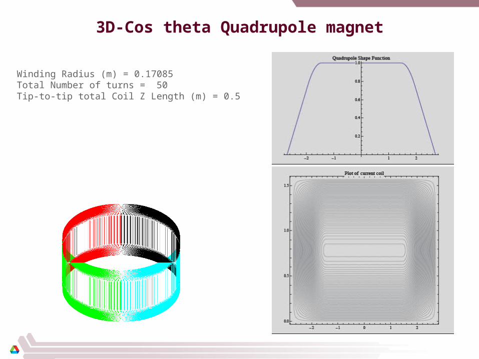
3D-Cos theta Quadrupole magnet

Winding Radius (m) = 0.17085Total Number of turns = 50Tip-to-tip total Coil Z Length (m) = 0.5

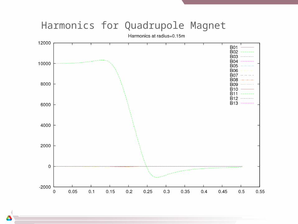
Harmonics for Quadrupole Magnet

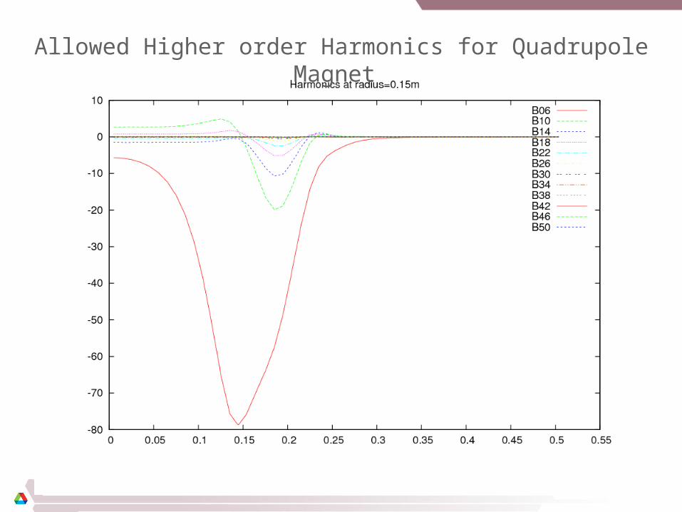
Allowed Higher order Harmonics for Quadrupole Magnet

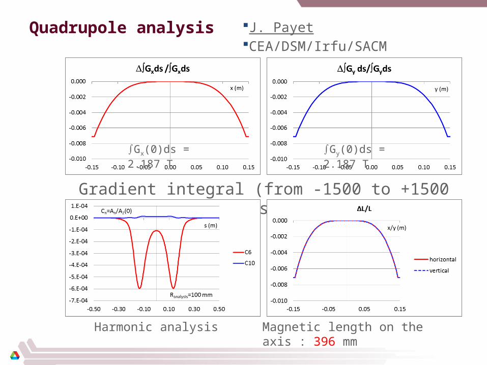
Quadrupole analysis

Magnetic length on the axis : 396 mmHarmonic analysis

Gradient integral (from -1500 to +1500 mm) homogeneities (red x, blue y)

Gx(0)ds = 2.187 T Gy(0)ds = 2.187 T

J. PayetCEA/DSM/Irfu/SACM

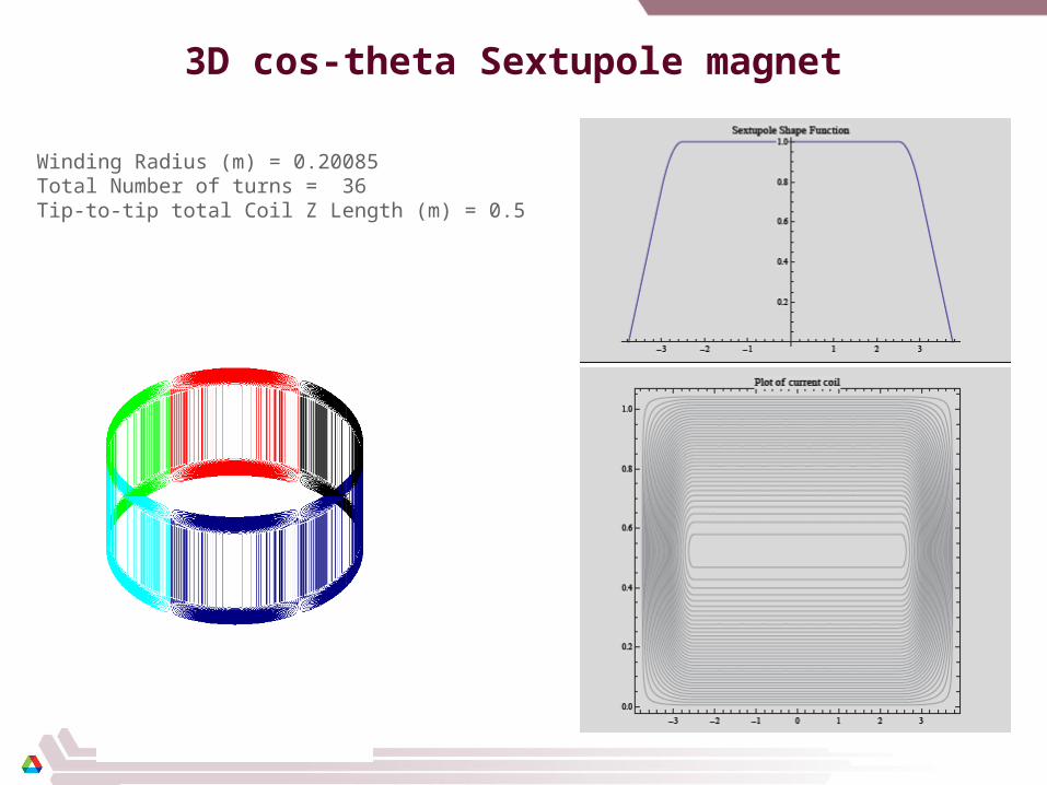
3D cos-theta Sextupole magnet

Winding Radius (m) = 0.20085Total Number of turns = 36Tip-to-tip total Coil Z Length (m) = 0.5

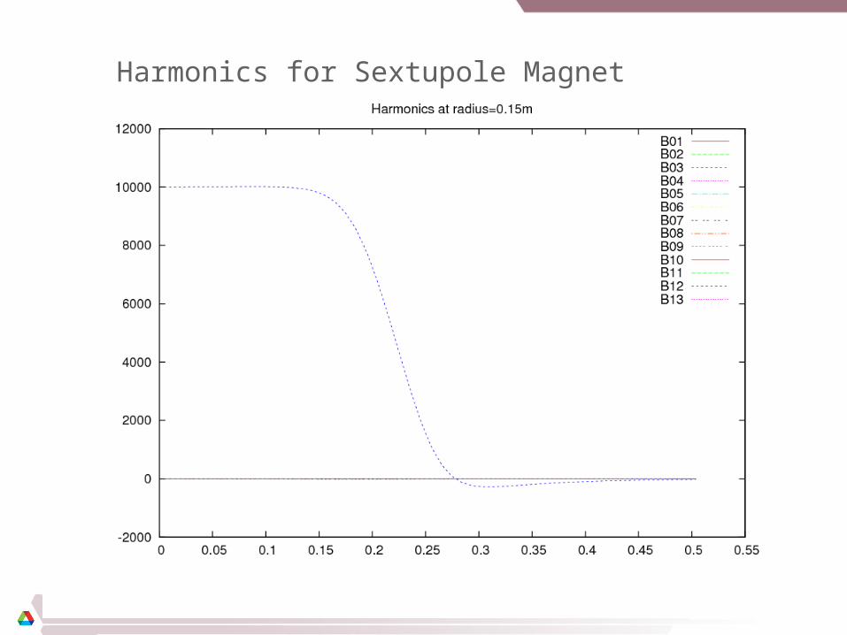
Harmonics for Sextupole Magnet

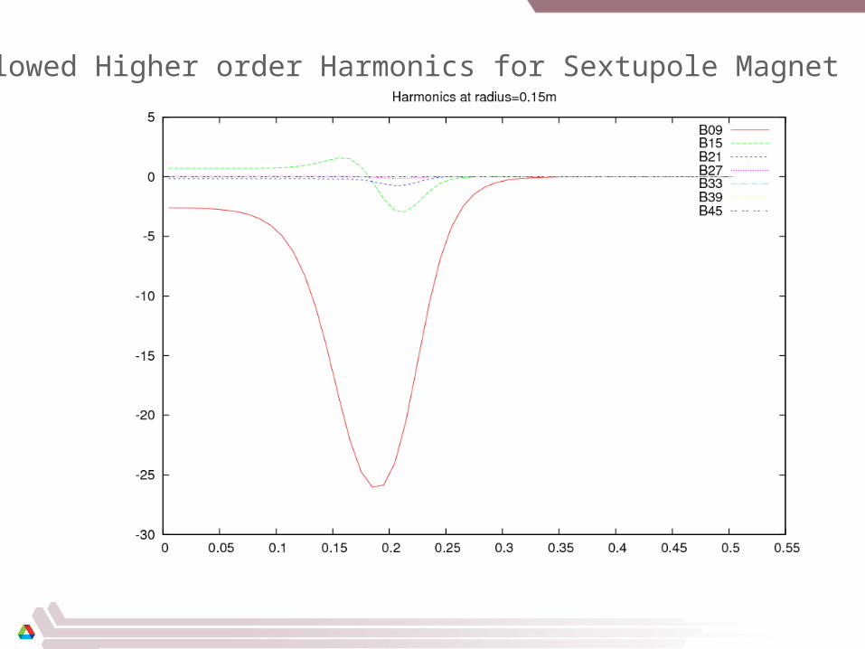
Allowed Higher order Harmonics for Sextupole Magnet

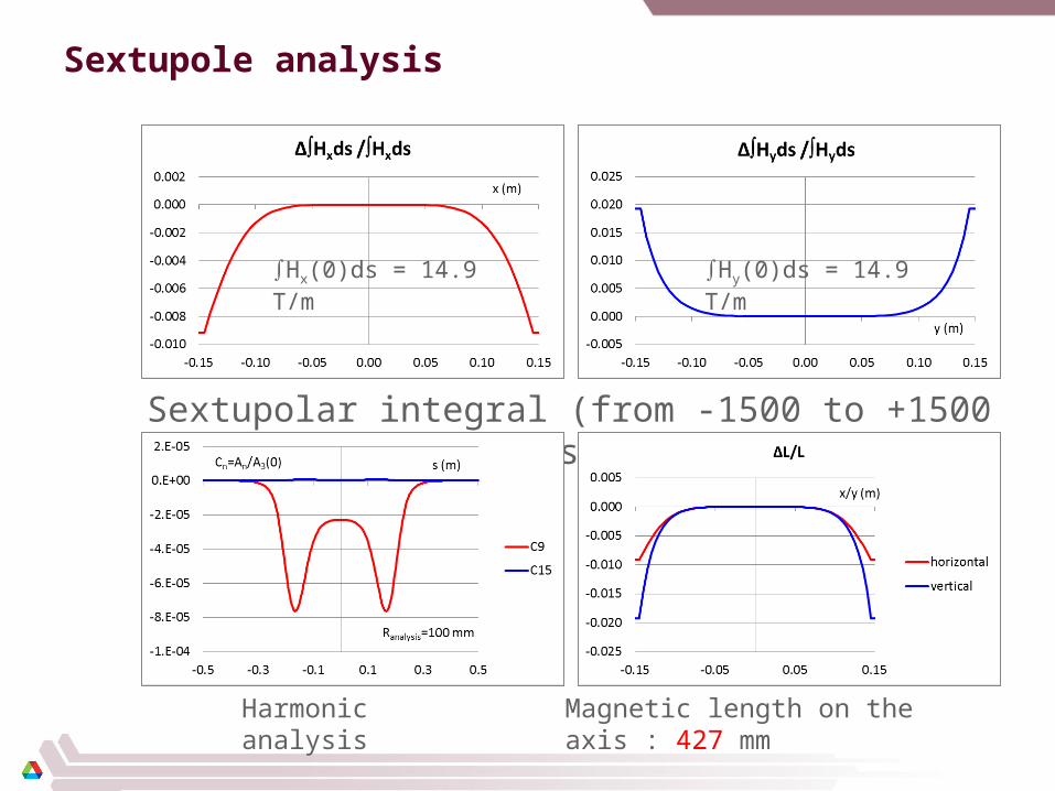
Sextupole analysis

Magnetic length on the axis : 427 mmHarmonic analysis

Sextupolar integral (from -1500 to +1500 mm) homogeneities (red x, blue y)

Hx(0)ds = 14.9 T/m Hy(0)ds = 14.9 T/m

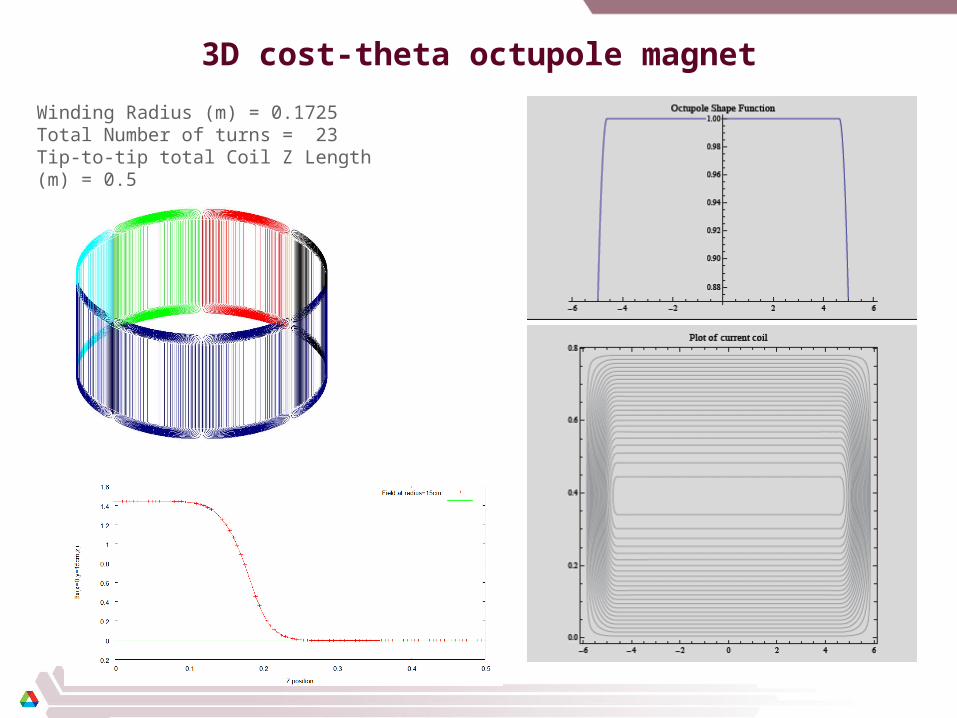
3D cost-theta octupole magnet

Winding Radius (m) = 0.1725Total Number of turns = 23Tip-to-tip total Coil Z Length (m) = 0.5

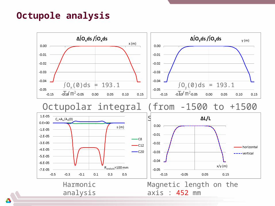
Octupole analysis

Magnetic length on the axis : 452 mmHarmonic analysis

Octupolar integral (from -1500 to +1500 mm) homogeneities (red x, blue y)

Ox(0)ds = 193.1 T/m2 Oy(0)ds = 193.1 T/m2

Conclusion

Simulation studies were done to look at the feasibility of Superconducting option for S3 multipole magnets

3D cos-theta magnets were chosen as the basis for magnet bids New coil models have been implemented in COSY-Infinity code

Thank You!

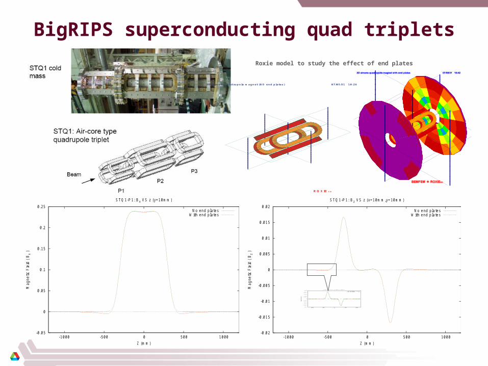
BigRIPS superconducting quad triplets

Roxie model to study the effect of end plates

ROXIE 9.0

07/05/31 10:263D aircore quadrupole magnet (NO end plates)

-0 .02

-0.015

-0.01

-0.005

0

0.005

0.01

0.015

0.02

-1000 -500 0 500 1000

Mag

netic

Fie

ld (

Bz

)

Z (m m )

STQ 1-P1: B z VS z (x=10m m ,y=10m m )

N o end p la tesW ith end p lates

-0 .02

-0.015

-0.01

-0.005

0

0 .005

0.01

0.015

0.02

-1000 -500 0 500 1000

Mag

netic Field ( B

z )

Z (m m )

STQ 1-P1: B z VS z (x=10m m ,y=10m m )

N o end p la tesW ith end p lates

-0 .05

0

0.05

0.1

0.15

0.2

0.25

-1000 -500 0 500 1000

Mag

netic

Fie

ld (

Bx

)

Z (m m )

STQ 1-P1: B x VS z (y=10m m )

N o end p la tesW ith end p lates

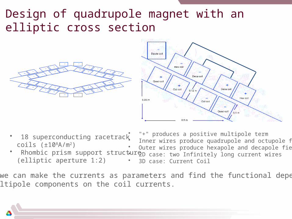
Design of quadrupole magnet with an elliptic cross section

• 18 superconducting racetrack coils (±108A/m2)• Rhombic prism support structure (elliptic aperture

1:2)

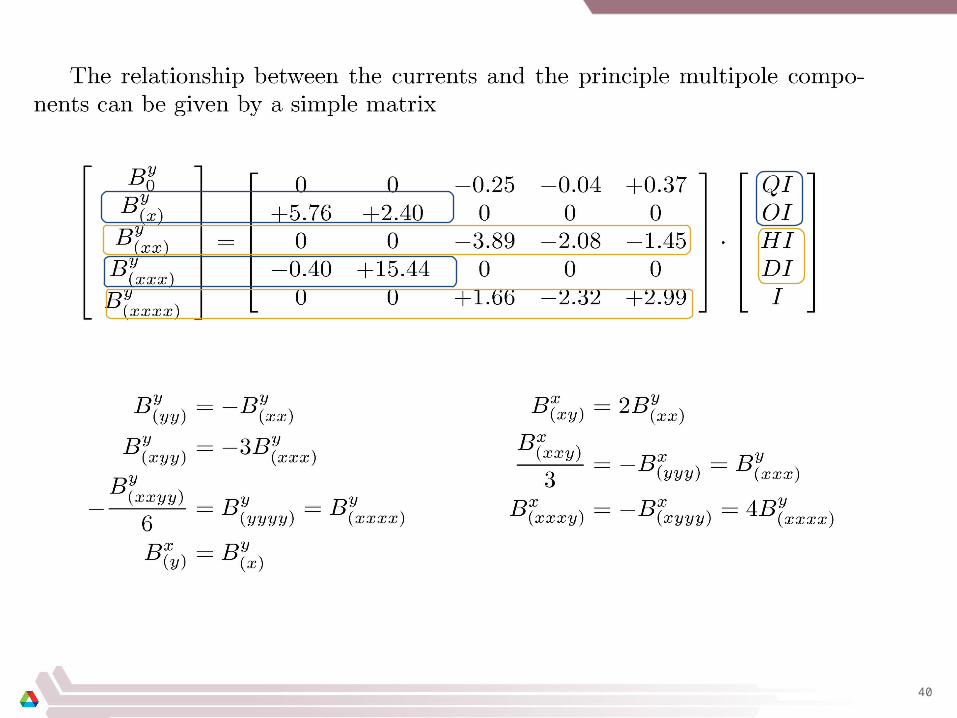
• "+" produces a positive multipole term• Inner wires produce quadrupole and octupole fields• Outer wires produce hexapole and decapole fields• 2D case: two Infinitely long current wires• 3D case: Current Coil

Using DA we can make the currents as parameters and find the functional dependence Of the multipole components on the coil currents.

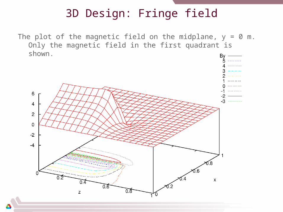
3D Design: Fringe field

The plot of the magnetic field on the midplane, y = 0 m. Only the magnetic field in the first quadrant is shown.

40

41

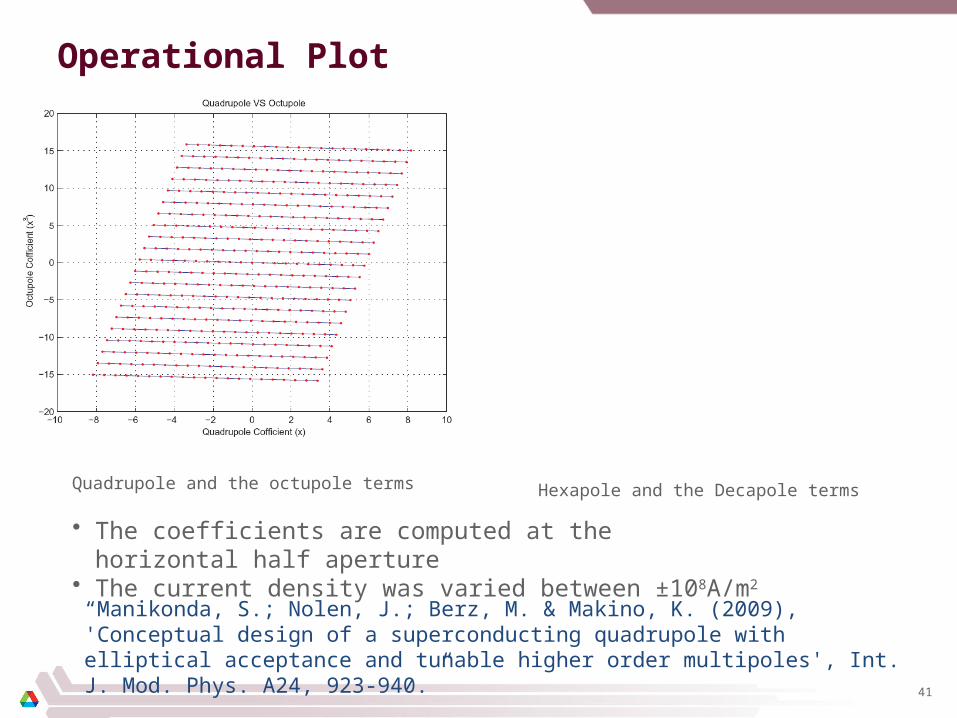
Operational Plot

Quadrupole and the octupole terms Hexapole and the Decapole terms

• The coefficients are computed at the horizontal half aperture• The current density was varied between ±108A/m2

“Manikonda, S.; Nolen, J.; Berz, M. & Makino, K. (2009), 'Conceptual design of a superconducting quadrupole with elliptical acceptance and tunable higher order multipoles', Int. J. Mod. Phys. A24, 923-940.”

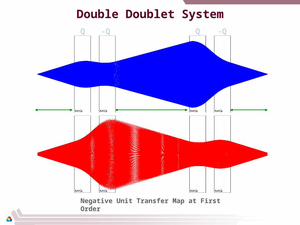
L 2L L

Q -Q Q -Q

Double Doublet System

Negative Unit Transfer Map at First Order

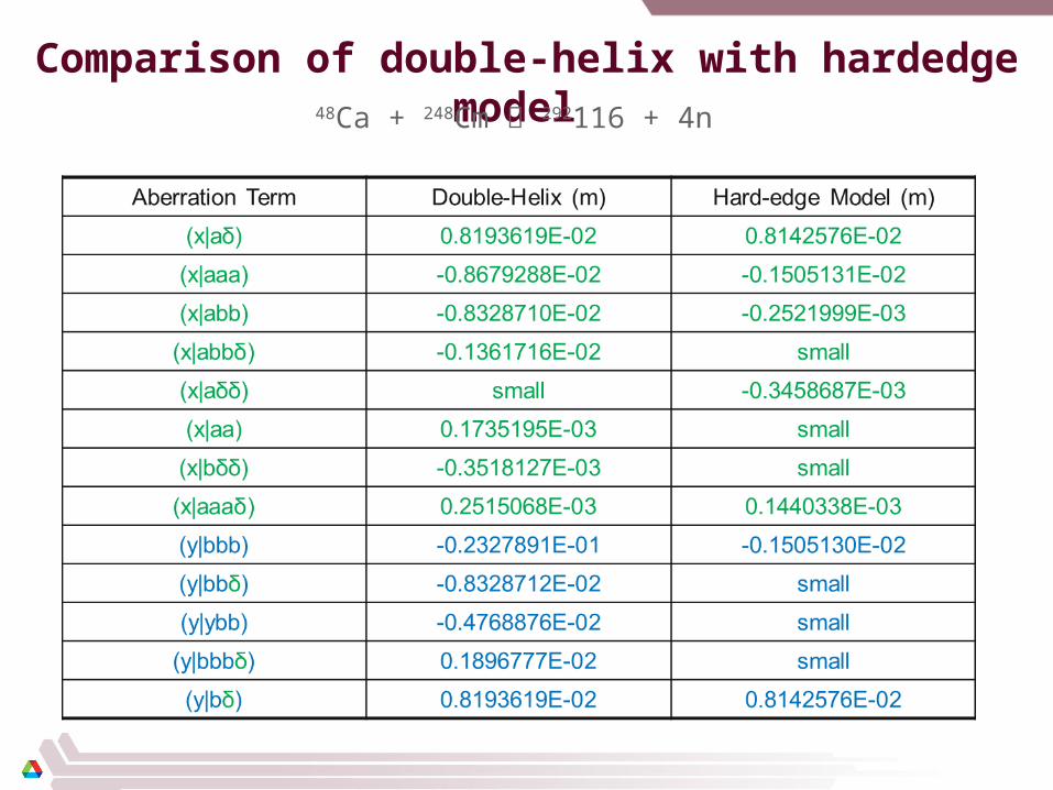
Comparison of double-helix with hardedge model 48Ca + 248Cm 292116 + 4n