RTEE Phase A Final Report - INFO - Home · ORNL/TM-2009/111 Real-Time Traffic Information for Emergency Evacuation Operations: Phase A Final Report December 2009 Prepared by Oscar

ORNL/TM-2009/111

Real-Time Traffic Information for Emergency Evacuation Operations: Phase A Final Report

December 2009 Prepared by Oscar Franzese, Ph.D. Senior Researcher, ORNL Li Zhang, Ph.D., P.E. Assistant Professor, MSU

DOCUMENT AVAILABILITY Reports produced after January 1, 1996, are generally available free via the U.S. Department of Energy (DOE) Information Bridge. Website http://www.osti.gov/bridge Reports produced before January 1, 1996, may be purchased by members of the public from the following source. National Technical Information Service 5285 Port Royal Road Springfield, VA 22161 Telephone 703-605-6000 (1-800-553-6847) TDD 703-487-4639 Fax 703-605-6900 E-mail [email protected] Website http://www.ntis.gov/support/ordernowabout.htm Reports are available to DOE employees, DOE contractors, Energy Technology Data Exchange (ETDE) representatives, and International Nuclear Information System (INIS) representatives from the following source. Office of Scientific and Technical Information P.O. Box 62 Oak Ridge, TN 37831 Telephone 865-576-8401 Fax 865-576-5728 E-mail [email protected] Website http://www.osti.gov/contact.html

This report was prepared as an account of work sponsored by an agency of the United States Government. Neither the United States Government nor any agency thereof, nor any of their employees, makes any warranty, express or implied, or assumes any legal liability or responsibility for the accuracy, completeness, or usefulness of any information, apparatus, product, or process disclosed, or represents that its use would not infringe privately owned rights. Reference herein to any specific commercial product, process, or service by trade name, trademark, manufacturer, or otherwise, does not necessarily constitute or imply its endorsement, recommendation, or favoring by the United States Government or any agency thereof. The views and opinions of authors expressed herein do not necessarily state or reflect those of the United States Government or any agency thereof.

ORNL/TM-2009/111

Southeast Region Research Initiative

REAL-TIME TRAFFIC INFORMATION FOR EMERGENCY EVACUATION OPERATIONS: PHASE A FINAL REPORT

Authors Oscar Franzese, ORNL (Co-PI)

Li Zhang, MSU (PI) Anas M. Mahmoud, MSU

Mary Beth Lascurain, ORNL Yi Wen, MSU

Date Published: December 2009

Prepared by OAK RIDGE NATIONAL LABORATORY

Oak Ridge, Tennessee 37831-6283 managed by

UT-BATTELLE, LLC for the

U.S. DEPARTMENT OF ENERGY under contract DE-AC05-00OR22725

AND Mississippi Transportation Research Center

Department of Civil and Environmental Engineering Mississippi State University Mississippi State, MS 39762

This page intentionally left blank.

iii

CONTENTS

Page CONTENTS ..........................................................................................................................................iii LIST OF FIGURES................................................................................................................................ v LIST OF TABLES ...............................................................................................................................vii ACRONYMS ........................................................................................................................................ ix EXECUTIVE SUMMARY...................................................................................................................xi 1. INTRODUCTION/BACKROUND............................................................................................... 1

1.1 PROJECT OBJECTIVES..................................................................................................... 2 1.2 PROJECT BENEFITS.......................................................................................................... 4 1.3 TECHNOLOGY TRANSFER ............................................................................................. 6

2. LABORATORY TESTS ............................................................................................................... 9 2.1 INTRODUCTION................................................................................................................ 9 2.2 CONTROLLED TESTS..................................................................................................... 11 2.3 CONTROLLED TESTS SUMMARY AND CONCLUSIONS......................................... 38

3. FIELD OPERATION TESTS...................................................................................................... 41 3.1 INTRODUCTION.............................................................................................................. 41 3.2 KNOXVILLE, TENNESSEE FOT (APRIL 2008) ............................................................ 42 3.3 STARKVILLE, MISSISSIPPI FOT (MAY 2008)............................................................. 50 3.4 FOT SUMMARY AND CONCLUSIONS ........................................................................ 61

4. NATIONAL TRANSPORTATION COMMUNICATIONS FOR ITS PROTOCOL DEVELOPMENT FOR PROTOTYPE SENSORS ............................................................................. 63

4.1 OBJECTIVE....................................................................................................................... 63 4.2 NTCIP FRAMEWORK STRUCTURE ............................................................................. 63 4.3 PROJECT IMPLEMENTATION....................................................................................... 66 4.4 TESTING ........................................................................................................................... 73 4.5 NTCIP SUMMARY AND CONCLUSIONS .................................................................... 74

5. SUMMARY, CONCLUSIONS AND FUTURE RESEARCH................................................... 75 5.1 LABORATORY AND FIELD OPERATIONAL TESTS SUMMARY............................ 75 5.2 NTCIP DEVELOPMENT SUMMARY ............................................................................ 77 5.3 CONCLUSIONS ................................................................................................................ 78 5.4 FUTURE RESEARCH AND DEVELOPMENT............................................................... 78

6. ACKNOWLEDGEMENTS......................................................................................................... 81 7. BIBLIOGRAPHY........................................................................................................................ 83 APPENDIX A. PROJECT ENDORSEMENT FROM OUTSIDE ORGANIZATIONS.................... 85


v

LIST OF FIGURES

Figure Page Figure 1 Evacuation Operations Process ................................................................................................ 1 Figure 2 Sensor Deployment .................................................................................................................. 2 Figure 3 Traffic Sensor System for Emergency Evacuations................................................................. 3 Figure 4 Prototype Sensor Showing Controllers, GPS, Power Supply and Communication Box ......... 5 Figure 5 NTRC Building and Parking Lots.......................................................................................... 10 Figure 6 Schematic Diagram of the NTRC Main Parking Lot............................................................ 10 Figure 7 Sensor Box and Deployed Detector ....................................................................................... 10 Figure 8 Sensors Set-up at the NTRC Main Parking Lot (First Laboratory Test)................................ 12 Figure 9 Laboratory Test 1 Round 2 Travel Time Differences Frequency Distribution (GT and P Paired Data) - Histogram and Box Plot (TT Diff in sec)...................................................................... 18 Figure 10 Laboratory Test 1 Round 2 Travel Time Differences Frequency Distribution (GT and P Paired Data) - Histogram and Box Plot (Zoomed around the Mean of the Distribution of TT Diff; TT Diff in sec)............................................................................................................................................ 19 Figure 11 Laboratory Test 1 Revised Round 2 Travel Time Differences Frequency Distribution (GT and P Paired Data) - Histogram and Box Plot, Excluding Four Far Outliers (TT Diff in sec)............. 19 Figure 12 Sensor Setup at the NTRC Main Parking Lot (Second Laboratory Test) ............................ 22 Figure 13 Inductive Signatures Captured by the Prototype Sensors during the 2nd Laboratory Test.. 28 Figure 14 Prototype and “Ground-Truth” Travel Time Information (Second Laboratory Test Series 1 – Round 1 – Segment S1-S2) ............................................................................................................... 29 Figure 15 Sensor Setup at the NTRC Main Parking Lot (Third Laboratory Test)............................... 31 Figure 16 Reported Spatial Location of Sensor 1................................................................................. 33 Figure 17 Reported Spatial Location of Sensor 2................................................................................. 33 Figure 18 Reported Spatial Location of Sensor 3................................................................................. 34 Figure 19 Real-Time Traffic Data Collected by Sensor 1.................................................................... 35 Figure 20 Real-Time Traffic Data Collected by Sensor 2.................................................................... 36 Figure 21 Real-Time Traffic Data Collected by Sensor 3.................................................................... 37 Figure 22 Tennessee FOT Prototype Sensors and GT Infrared Sensor Placement ............................. 42 Figure 23 Tennessee FOT Deployed Prototype Sensor 2(ORNL 2) and GT Infrared Sensor 2 .......... 42 Figure 24 Tennessee FOT GT Data Gathering Device ........................................................................ 43 Figure 25 Examples of Images Taken with Camera 2 (Tennessee FOT)............................................. 44 Figure 26 Location of “Zones” for Camera 1 (Tennessee FOT). ......................................................... 45 Figure 27 Location of “Zones” for Camera 2 (Tennessee FOT) .......................................................... 45 Figure 28 Location of “Zones” for Camera 3 (Tennessee FOT) .......................................................... 46 Figure 29 Real-Time Traffic Information Provided by the Prototype Sensors (Tennessee FOT) ....... 47 Figure 30 Tennessee FOT Ground-Truth and Prototype Travel Time ................................................. 48 Figure 31 Tennessee FOT Travel Time Differences Frequency Distribution (GT and P Paired Data) Histogram and Box Plot (TT Diff in sec) ............................................................................................. 49 Figure 33 Mississippi FOT Prototype Sensors and GT Camera Placement ......................................... 52 Figure 34 Mississippi FOTs Sensor Deployment (ORNL 1) ............................................................... 53 Figure 36 Mississippi FOT 1 Real-Time Traffic Information Provided by the Prototype Sensors...... 55 Figure 37 Mississippi FOT 1 Real–time Geospatial Location of Sensors............................................ 55 Figure 38 MSU FOT 1 Traffic and Turning Movement Counts .......................................................... 57 Figure 39 MSU FOT 1: Segment 1-2 Travel Time Differences Frequency Distribution (GT and P Paired Data) - Histogram and Box Plot (TT Diff in sec)...................................................................... 59 Figure 40 MSU FOT 1: Segment 2-3 Travel Time Differences Frequency Distribution (GT and P Paired Data) - Histogram and Box Plot (TT Diff in sec)...................................................................... 59 Figure 41 NTCIP Architecture (NTCIP 9001) ..................................................................................... 64

vi

Figure 42 NTCIP Role in the ITS National Architecture (NTCIP 9001) ............................................ 65 Figure 43 Basic SOAP Operation over HTTP ..................................................................................... 67 Figure 44 NTCIP Implementation using SOAP- Architectural Design............................................... 67 Figure 45 IST Standard DB Schema.................................................................................................... 69 Figure 46 IST Data Field in SectionStatisticsPacket ........................................................................... 70 Figure 47 Data Table within MSU NTCIP Server............................................................................... 71 Figure 48 SOAP Client’s GUI ............................................................................................................. 72 Figure 49 NTCIP SOAP Interface in a Real-world Implementation ................................................... 73

vii

LIST OF TABLES Table Page Table 1 Data Collection Spreadsheet ................................................................................................... 12 Table 2 Random Travel Patterns for Veh1 and Veh2 .......................................................................... 14 Table 3 Data Collection Spreadsheet for TP1/TP2 .............................................................................. 14 Table 4 Laboratory Test 1 Results: All Data by Test Series and Test Round ...................................... 16 Table 5 Laboratory Test 1 Results: Matched Observations by Test Series and Test Round................ 16 Table 6 Laboratory Test 1-Test Series 2 Results: Matched Observations by Vehicle and Test Round17 Table 7 Laboratory Test 1-Revised Round 2 Travel Time Differences Distribution Summary Statistics (GT and P Paired Data) ........................................................................................................................ 20 Table 8 Sensor Crossing Order for Veh1 and Veh2............................................................................. 23 Table 9 Random Travel Patterns for Veh1 and Veh2 (Delay in Seconds)........................................... 24 Table 10 Laboratory Test 2 Results: All Data by Test Series and Test Round .................................... 25 Table 11 Laboratory Test 2 Results: Matched Observations by Test Series and Test Round.............. 26 Table 12 Laboratory Test 2-Segment S1-S2: Matched Observations by Vehicle, Test Series and Test Round ................................................................................................................................................... 27 Table 13 Travel Time Differences Distribution Summary Statistics (GT and P Paired Data for Test Series 1 – Round 1) .............................................................................................................................. 29 Table 14 Random Travel Patterns for Veh1 and Veh2 (Delay in Seconds)......................................... 32 Table 15 Tennessee FOT Data Collection Spreadsheet ....................................................................... 43 Table 16 Tennessee FOT Results: Randomly Selected Travel Time Data by Date ............................. 47 Table 17 Tennessee FOT Results: Randomly Selected Matched Travel Time Data by Date .............. 48 Table 18 Tennessee FOT Travel Time Differences Distribution - Summary Statistics (GT and P Paired Data) .......................................................................................................................................... 50 Table 19 MSU FOT 1 Results: Travel Time Data by Segment............................................................ 58 Table 20 MSU FOT 1 Results: Matched Travel Times........................................................................ 58 Table 21 MSU FOT 1: Segment 1-2 Travel Time Differences Distribution Summary Statistics (GT and P Paired Data) ................................................................................................................................ 60 Table 22 MSU FOT 1: Segment 2-3 Travel Time Differences Distribution Summary Statistics (GT and P Paired Data) ................................................................................................................................ 60


ACRONYMS ASP Active Server Pages ATM Asynchronous Transfer Mode CCC Command and Control Center CI Confidence Interval C2C Center-to-Center C2C WG Center-to-Center Working Group C2F Center-to-Field CSU/DSU Channel Service Unit/Data Service Unit CORBA Common Object Request Broker Architecture C2I Command, Control, and Interoperability COP Common Operating Picture CTA Center for Transportation Analysis DATEX Data Exchange Protocol DB Database DHS Department of Homeland Security DOT Department of Transportation ETMCC External Traffic Management Center Communications FEMA Federal Emergency Management Agency FHWA Federal Highway Administration FOT Field Operation Test FTP File Transfer Protocol GIS Geographic Information Systems GPS Global Positioning System GT Ground Truth GUI Graphical User Interface Ha Alternative Hypothesis HDLC High-Level Data Link Control Ho Null Hypothesis HTTP Hyper Text Transfer Protocol IIS Internet Information Services IP Internet Protocol IQR Interquartile Range ISO International Organization of Standards IST Inductive Signature Technologies, Inc. ITS Intelligent Transportation Systems KTL Kelly Gene Cook Transportation Laboratories MDOT Mississippi Department of Transportation MEMA Mississippi Emergency Management Agency MS Microsoft MSU Mississippi State University MTRC Mississippi Transportation Research Center NTRC National Transportation Research Center NTCIP National Transportation Communication for ITS Protocol OREMS Oak Ridge Evacuation Modeling System ORNL Oak Ridge National Laboratory OSI Open System Interconnection P Prototype PC Passenger Car

PPP Point-to-Point Protocol R&D Research and Development SE Standard Error SERRI Southeast Region Research Initiative S&T Science and Technology SW Stopwatch USB Universal Serial Bus U.S. DOT United States Department of Transportation SD Standard Deviation SNMP Simple Network Management Protocol SOAP Simple Object Access Protocol SQL Structured Query Language STMP Simple Transportation Management Protocol SUV Suburban Utility Vehicle TCP Transmission Control Protocol TCP/IP Transmission Control Protocol/Internet Protocol TCIP Transit Communications Interface Profiles TFTP Trivial File Transfer Protocol TMC Traffic Management Center TP Travel Pattern TT Travel Time UDP User Datagram Protocol Veh Vehicle VMS Variable Message Signs VS.NET Microsoft Visual Studio [dot] NET W3C World Wide Web Consortium WSDL Web Service Description Language XML eXtensible Markup Language

xi

EXECUTIVE SUMMARY There are many instances in which it is possible to plan ahead for an emergency evacuation (e.g., an explosion at a chemical processing facility). For those cases, if an accident (or an attack) were to have happened, then the best evacuation plan for the prevailing network and weather conditions would be deployed. In other cases (e.g., the derailment of a train transporting hazardous materials), there may not be any previously developed plan to be implemented, and decisions must be made on an ad-hoc basis on how to proceed with an emergency evacuation. In both situations, the availability of real-time traffic information plays a critical role in the management of the evacuation operations. To improve public safety during a vehicular emergency evacuation it is necessary to detect losses of road capacity (due to incidents, for example) as early as possible. Once these bottlenecks are identified, re-routing strategies must be determined in real-time and deployed in the field to help dissipate the congestion and increase the efficiency of the evacuation. Due to cost constraints, only large urban areas have traffic sensor deployments that permit access to some sort of real-time traffic information; any evacuation taking place in any other areas of the country would have to proceed without real-time traffic information. The latter is the focus of this project. The main objective of this SERRI/DHS (Southeast Region Research Initiative/Department of Homeland Security) sponsored project is to improve the operations during a vehicular emergency evacuation anywhere by using newly developed real-time traffic-information-gathering technologies to assess traffic conditions and therefore to potentially detect incidents on the main evacuation routes. The benefits that this project will help realize relate to the response and recovery functions during an emergency evacuation involving large populations. Information gathering and distribution plays a critical role in the response phase because it is paramount to determine the status of the transportation system to help with the decision process and field operations (e.g., routing emergency vehicles around congested areas). The system developed in this project can collect and provide traffic information in real time for both the system managers (transportation agencies, emergency management agencies, law enforcement agencies, fire and rescue agencies, emergency medical service providers, 911 dispatchers, and towing companies) and the public. The ultimate goal is to create a system which emergency management agencies, and/or other public safety organizations, can rapidly deploy anywhere to help manage traffic operations during emergency evacuations. This is a very critical and necessary system as pointed out by experts such as Ms. K. Vasconez, Team Leader of the Federal Highway Administration’s (FHWA’s) Emergency Transportation Operations group (see Appendix A). Phase A of the project consisted of the development and testing of a prototype system composed of sensors that are engineered in such a way that they can be rapidly deployed in the field where and when they are needed. Each one of these sensors, developed by IST, Inc (Inductive Signature Technologies, Inc., a Tennessee-based company), is also equipped with their own power supply and a GPS (Global Positioning System) device to auto-determine its spatial location on the transportation network under surveillance. The system is capable of assessing traffic parameters by identifying and re-identifying vehicles in the traffic stream as those vehicles pass over the sensors. The system of sensors transmits, through wireless communication, real-time traffic information (travel time and other parameters) to a command and control center (CCC) via an NTCIP (National Transportation Communication for Intelligent Transportation Systems Protocol) -compatible interface. As an alternative, an existing NTCIP-compatible system accepts the real-time traffic information mentioned and broadcasts the traffic information to emergency managers, the media and the public via the existing channels.

xii

The first part of this project centered on the development of the prototype system and a methodology to conduct an assessment of its capabilities. Subsequently, the project team conducted a series of tests, both in a controlled environment and in the field, to study the feasibility of rapidly deploying the system of traffic sensors and to assess its ability to provide real-time traffic information during an emergency evacuation. Specifically, the tests were aimed at evaluating the performance of the system of sensors under various traffic and weather conditions and roadway environments. The controlled tests (i.e., deployment and testing of the prototype system in a parking lot with very limited traffic) were performed first, and the results obtained served as the basis to identify flaws in the system and make the necessary corrections to the prototype. The working prototype that resulted from these Research and Development (R&D) activities was then subject to series of real-world environment tests (Field Operation Tests, or FOTs). Those FOTs, which were aimed at studying the reliability and accuracy of the system in a more prolonged time frame, were conducted at two sites: Knoxville, Tennessee (using traffic in and out of an office complex during an entire week) and Mississippi State University (MSU) Starkville, Mississippi campus (using traffic generated during university and high school commencements). The latter provided the opportunity to create scenarios that have many characteristics (e.g., congested roads) that are similar to those encountered during a real evacuation, particularly from the standpoint of traffic. The results of the tests showed that the system had a very good reliability (90%+ in laboratory tests and 55-85% in FOTs) and accuracy (95%+ in laboratory tests and 90%+ in FOTs). An interface using the NTCIP standard was also developed to transmit traffic information to existing and future traffic management centers (TMCs). The NTCIP-compatible interface enables future deployment of the system not only in the Southeast Region, but also anywhere in the U.S. because NTCIP is the national standard that is adopted by any TMC publicly funded within the U.S. The results of the first phase of the project indicated that the prototype sensors are reliable and accurate for the type of application that is the focus of this project. During an emergency, these sensors would be deployed by law enforcement or emergency management personnel, who are likely to be performing many other activities. Therefore, to make this a viable tool to be used in emergency evacuations, the loop detectors (i.e., the component of each sensor which lies on the pavement and captures the vehicles’ inductive “signatures”) should be easy to deploy and the system should work on a “fire-and-forget” regime. That is, the emergency personnel involved in the deployment of the system should only be required to place the loop detectors on the pavement (e.g., by rolling the loop detector across the roadway) at key points within the evacuating area and to connect them to the sensor box. After that, the system of sensors should self-configure, calibrate, start gathering data, transmit traffic parameters (travel time) to the designated emergency operations center, and be ready to interact with other systems. The project team focused on researching and exploring sensor accuracy on laboratory and real-world conditions. In a real evacuation case, the balance between accuracy and the number of deployed sensors, which determine the cost of data collection, is of fundamental importance. A poorly designed deployment of the sensors may not capture the key parameters needed to optimize the traffic operations during an evacuation, and could impose higher costs than necessary. Therefore, one key objective of future research is the determination of the optimum location of the sensors. The integration of the system with TMCs and CCCs through the NTCIP interface will make it possible for emergency managers and the public to receive travel-time information in real time. Although the NTCIP interface is ready at this point, the entire proposed system needs to be tested with an existing TMC. The project team has already identified potential locations and TMC systems to conduct future inter-agency tests.

xiii

The sensor deployability, location, and integration with other systems are issues which could be addressed in a future phase of this project.

xiv


1

1. INTRODUCTION/BACKROUND There are many instances in which it is possible to plan ahead for an emergency evacuation (e.g., a radiological accident at a nuclear plant or an explosion at a chemical processing facility). For those cases, if an accident (or an attack) were to happen, then the best evacuation plan for the prevailing roadway network and weather conditions would be deployed (if evacuation is the optimal protective action). Traffic conditions, collected in real-time, would be provided to the control center to assess if operations are proceeding as planned, or if changes are needed to assure the safety of the evacuating public. In other cases (for example, the derailment of a train transporting hazardous materials), there may not be any previously developed plan to be implemented, and decisions must be made on an ad-hoc basis on how to proceed with an emergency evacuation. In both situations, the availability of real-time traffic information plays a critical role in the management of the evacuation operations. During a vehicular emergency evacuation, and to improve public safety, it is necessary to detect losses of road capacity (due to incidents, for example) as early as possible. Once these bottlenecks are identified, re-routing strategies must be determined in real-time and deployed in the field to help dissipate the congestion and to increase the efficiency of the evacuation. The deployment of these re-routing strategies requires that information be distributed to the evacuating population in real-time and, as much as possible, to specific locations so traffic can self-divert to the new routes. Figure 1 shows this process in a graphical form.

Evacuation Plan Deployment

Field Data CollectionReal-time Traffic Conditions

Road Conditions

Evacuation MonitoringIncident Detection

Determination of Optimal Traffic Re-routing Strategy

Information Distributionto Evacuating Population

End of Evacuation

Determination of Optimal Protective ActionEvacuation

Shelter in Place

Evacuation Plan Deployment

Field Data CollectionReal-time Traffic Conditions

Road Conditions

Evacuation MonitoringIncident Detection

Determination of Optimal Traffic Re-routing Strategy

Information Distributionto Evacuating Population

End of Evacuation

Determination of Optimal Protective ActionEvacuation

Shelter in Place

Figure 1 Evacuation Operations Process

2

1.1 PROJECT OBJECTIVES 1.1.1 Objectives

The main objective of this SERRI/DHS (Southeast Region Research Initiative/Department of Homeland Security) sponsored project is to improve the operations during a vehicular emergency evacuation anywhere in the country by using newly developed real-time traffic-information-gathering technologies to assess traffic conditions and to detect incidents on the main evacuation routes. The ultimate goal is to create a system that emergency management agencies, and/or other public safety organizations, can rapidly deploy anywhere to help manage traffic operations during emergency evacuations.

The prototype system is composed of sensors developed by Inductive Signature Technologies (IST, a

Tennessee-based company). They are engineered in such a way that they can be rapidly deployed in the field—e.g., taped to the roadway or through other means—at key points on the transportation network that need to be monitored (e.g., see the blue rectangles in Figure 2, which shows a schematic deployment of the sensors in an otherwise non-instrumented urban area). Those fast-deployable sensors (see Figure 3) are equipped with GPS (Global Position System) devices to auto-determine their spatial location on the transportation network under surveillance, and are capable of assessing traffic parameters by identifying specific vehicles’ electric-magnetic signatures in the traffic stream. The system of sensors transmit, through wireless communication, real-time traffic information to a command and control center (CCC), including travel time and traffic volumes on each instrumented segment of roadway.

Figure 2 Sensor Deployment

The traffic information collected, once processed, can be published as a National Transportation Communication for Intelligent Transportation Systems (ITS) Protocol (NTCIP) compatible message (in this case, NTCIP 2306) on the Internet. Any existing NTCIP-compatible Traffic Management Center (TMC) requests for real-time traffic information are granted and the traffic information is then transmitted to the TMC in the form of a Simple Object Access Protocol (SOAP) message. The TMCs broadcast the critical traffic information to the emergency managers, the media and the public via existing channels such as the 511 traffic information, television, radio, text messages and variable message signs (VMS).

3

NTCIPNTCIP

Figure 3 Traffic Sensor System for Emergency Evacuations

1.1.2 Partners

The team assembled for this project consisted of Oak Ridge National Laboratory (ORNL) researchers from the Center for Transportation Analysis (CTA) of the Energy and Transportation Science Division, Mississippi State University (MSU) researchers from their civil engineering department, and researchers from the private sector. CTA is a transportation research center at ORNL that conducts innovative research in transportation with a focus on developing and applying advanced computational techniques, analytical methods and information resources to improve economic and energy efficiency, environmental quality, mobility, national security and public safety. Relevant to this project, and through the Chemical Stockpile Emergency Preparedness Program of the Federal Emergency Management Agency (FEMA) and the U.S. Army, CTA has developed the Oak Ridge Evacuation Modeling System (OREMS), a traffic simulation model that can facilitate emergency routing and evacuation planning in practical applications. With a mixture of technical and scientific backgrounds and diverse project sponsorship, CTA’s interdisciplinary approach to problem solving is one of its major strengths. CTA also houses a broad range of software systems on workstations in both the UNIX® and Windows® environments and is also able to take advantage of a variety of software development tools as well as mainframe computers and supercomputers at ORNL facilities. MSU holds a strong transportation engineering program, both in transportation education and research. The Mississippi Transportation Research Center (MTRC), housed and administered within the Department of Civil and Environmental Engineering in the Bagley College of Engineering, was established at MSU in order for the university to provide a consistent line of communication with the Mississippi Department of Transportation (MDOT). The Kelly Gene Cook Transportation Laboratories (KTL) is a unique transportation research and education laboratory within the MTRC. The Kelly Gene Cook Foundation, civil engineering department, Bagley College of Engineering and MSU provided funding for this project (research laboratory and equipment).

4

IST has successful worked for over eight years on inductive signature-related vehicle detection, and classification and tracking projects; all of them related to permanent deployments. IST holds several key patents on inductive-loop vehicle signature technology. This technology was expanded and adapted to the needs of this project, which required a more challenging operational environment than permanent deployment settings.

1.2 PROJECT BENEFITS The benefits that this project may help realize are mainly related to the response and recovery functions during an emergency evacuation involving large populations. Information gathering and distribution play a critical role in the response phase because it is paramount to determine the status of the transportation system in order to help with the decision process and field operations (e.g., routing emergency vehicles around congested areas). The system developed in this project can collect and provide traffic information in real time for both the system managers (transportation agencies, emergency management agencies, law enforcement agencies, fire and rescue agencies, emergency medical service providers, 911 dispatchers and towing companies) and the public. The technology developed in this project will augment existing ITS deployments where available (usually freeways in large urbanized areas). For the remaining cases (e.g., arterials in instrumented urban areas, non-instrumented urban areas and rural areas) this technology may be the sole source of real-time traffic information during an emergency evacuation. Because the same technologies and capabilities used during the response stage are applicable to the recovery phase, the system developed in this project will also provide aid in that phase of an emergency. The successful development of the NTCIP-compatible interface enables the future deployment of the system to be utilized not only in the southeast region, but also anywhere in the U.S. because NTCIP is the national standard that is adopted by any TMC publicly funded within the U.S. The benefits of the NTCIP interface extend beyond the inter-agency cooperation. The TMCs provide channels for broadcasting the critical traffic information to the emergency managers, the media and the public. Integrating the emergency travel time with existing channels will cause less confusion among the public as well.

1.2.1 Phase A Research and Development The first phase of this project focused on conducting a series of tests and developing an NTCIP interface. The tests were performed both in a controlled environment and in the field, to study the feasibility of rapidly deploying a system of traffic sensors and to assess the system’s ability to provide real-time traffic information during an emergency evacuation. Specifically, the tests were aimed at assessing the performance of the system sensors under various “mounting” configurations, traffic and weather conditions and roadway environments. In order to accomplish these objectives, the test was divided into two stages with a parallel effort to develop an NTCIP interface. The first stage centered on the development of the prototype system and on a methodology to conduct a preliminary assessment of its feasibility and capabilities. A series of laboratory tests (i.e., deployment and testing of the prototype system in a controlled environment, such as a parking lot with very limited traffic) was performed, and the results obtained served as the basis to identify flaws in the system and to make the necessary corrections to the prototype. The working prototype that resulted from the Research and Development (R&D) performed in stage one (see Figure 4) was subjected to real-world environment tests (Field Operation Tests, or FOTs) during the subsequent stage. Those FOTs, which were aimed at studying the reliability and accuracy of the system in a more prolonged time frame, were conducted at two sites. The first site was in Knoxville, Tennessee

5

and used traffic in and out of an office complex during an entire week to compare the information provided from the sensors against “ground-truth” (GT) data. The second site was in Starkville, Mississippi at the MSU campus. This site included the areas surrounding a sports venue that was used on several occasions in May 2008 to celebrate university and high school commencements. These events, although not exactly the same as an emergency evacuation, provided the opportunity to create scenarios that have many characteristics (e.g., congested roads) that are similar to those encountered during a real evacuation, particularly from the standpoint of traffic.

Figure 4 Prototype Sensor Showing Controllers, GPS, Power Supply and Communication Box A parallel task focused on the development of an NTCIP-compatible interface.

1.2.1.1 Project Outcomes

The main outcomes of this 18-month project were: 1) the development of the system architecture for a fast deployable and portable traffic detection system for no-advanced-notice emergency evacuations; 2) the development and assembly of a field-tested prototype system consisting of three sensors that were able to identify/re-identify vehicles in real-time in a stream of traffic in order to generate travel time and other traffic parameters, as well as transmitting that information, also in real time, to any designated CCC; and 3) the development of a standardized interface for the prototype system that is compliant with the ITS National Architecture (U.S. DOT) and that will permit the system to be integrated with other hardware and information systems. 1.2.1.2 Linkage to DHS S&T Objectives This project addressed three main objectives of DHS Office of Science and Technology (S&T): 1) incident management, 2) information sharing, and 3) infrastructure protection.

6

Incident Management. The representative technology needs addressed by this project include: a) incident management enterprise system (Infrastructure Protection/Geophysical Division) and b) logistics management tool (Infrastructure Protection /Geophysical Division). The prototype system developed under this project can provide real-time travel-time and traffic information during any incident. Travel-time information is fundamental to any transportation logistics management tool and can improve the operation of large-scale emergency vehicular evacuations not only for the population at risk, but also for the emergency management personnel (e.g., helping with emergency vehicle route planning). Because the basic characteristic of the prototype system is that it can be quickly deployed anywhere, it can assist with the operations and management of incidents that have little or no advance notice. Information Sharing. The representative technology needs addressed by this project include: a) data fusion from multiple sensors into a Common Operating Picture (COP) (Command, Control, and Interoperability, C2I, Division), b) improved real-time data sharing of law enforcement information (C2I Division) and c) automated, dynamic, real-time data processing and visualization capability (C2I Division). The prototype system’s ability to collect real-time travel time and other traffic parameters would provide critical information to federal, state and local law enforcement agencies that could help to better manage any emergency that affects large geographical areas. The ability of the system to spatially and temporally tag the information gathered makes it easy to integrate with visualization systems using GIS (Geographic Information Systems) technologies. Infrastructure Protection. The representative technology needs addressed by this project include advanced, automated and affordable monitoring and surveillance technologies (C2l Division). The prototype system provides surveillance and monitoring capabilities that are advanced (e.g., travel time and other traffic parameters that are not available through traditional traffic detection), accessible to DHS/DOT and other agencies (e.g., the system broadcasts the traffic surveillance information to any designated CCC or TMC) and affordable (e.g., the system can be deployed temporarily where needed and re-used in other areas).

1.3 TECHNOLOGY TRANSFER

For the system developed in this project, technology transfer involves two different aspects. The first one deals with the technical feasibility of the technology (which was the main purpose of this study), and more specifically with its integration into existing (and future) systems. This project addressed this first set of issues through the integration of different “off-the-shelve” positional and communications technologies with traffic sensors that although innovative, have already been deployed and proven in other settings. The project team worked directly with the private sector partner (IST) to resolve those issues; creating an integrated system that is self-contained and capable of generating real-time traffic information that is spatially labeled and therefore can be displayed within any GIS platform. The role that the project team played was in helping to develop and test the proposed prototype system created with technology that was already in the private domain, thus accelerating the technology transfer process. The results of this research have shown that the proposed technology is not only feasible, but even at the current development stage is accurate and reliable. Also, under the present project, an NTCIP interface was developed for the prototype system assuring its interoperability with existing and future traffic information gathering and distribution systems.

7

The second aspect that needs to be solved to complete the technology transfer process and have a system that is ready to be mass-produced involves issues related to the physical deployment of the system of sensors. From the inception of this project it was understood that the loop detectors (the actual piece of hardware that is placed on the roadway and that reads the inductive signature of the vehicles) would have to be deployed by law enforcement or other emergency management personnel, who are very likely to be extremely busy during a catastrophic event. The overriding criterion, therefore, is to create a system with “deploy and forget” sensors that could be easily and rapidly positioned in the field. The focus of the second phase of this project will be on this component of the system (see the “Future Research and Development” section at the end of this report). Once these deployability issues are solved, the technology transfer will be complete.

8


9

2. LABORATORY TESTS 2.1 INTRODUCTION

The main focus of this phase of the project was on the development and fine-turning of the prototype sensors to collect and distribute traffic information in real time. To achieve these objectives, a battery of tests was designed and conducted. Those tests were divided into two parts: 1) “laboratory environment” tests, i.e., tests that were conducted under highly controlled conditions; and 2) FOTs, i.e., tests that were conducted under similar conditions to those that the sensors will encounter when operating under “real-world” conditions. This chapter describes the laboratory environment tests (three series of tests were conducted), while the next chapter focuses on the FOTs (five tests were conducted). In both cases, the testing of the prototype system involved three main tasks: the development of a testing methodology, the collection of data during the tests and the analysis of the information gathered. The basic testing methodology for the laboratory tests is described below with more and specific details added in the subsequent sections for each one of the three series of tests that were performed. The analysis of the collected data, also explained in detail below for each one of the three test series, was performed using a paired t-test and other statistical techniques to compare baseline measurements of the collected traffic parameters against the same traffic parameters reported by the prototype system. Where pertinent, confidence intervals (CIs) were constructed for these measurements to provide an assessment of the accuracy with which the proposed technology was able to measure traffic parameters. For both the laboratory and the FOT tests, some analysis of the data was performed concurrently with the tests (i.e., the data was analyzed as it was gathered or immediately thereafter) to allow making adjustments to both the data collection procedures and the prototype system itself. Any identified deficiencies in the prototype system were corrected in an expedient manner; subsequent tests were used to determine if the adjustments made to the prototype had been successful.

2.1.1 Testing Methodology Background The laboratory-environment testing methodology for the prototype system concentrated on the evaluation of different aspects of the system, including its capacity to collect and transmit traffic data, its ability to generate meaningful traffic parameters that are spatially tagged and the capability of the sensors to communicate among themselves and to a centralized system (e.g., CCC). In order to have a reasonably controlled environment to conduct these tests, the National Transportation Research Center (NTRC) building1 main parking lot was used. Although the building can be accessed anytime by the researchers working there, during weekends and holidays, very few vehicles access this parking lot, which made it an ideal place to test the prototype system. Figure 5 shows an aerial view of the building with the main parking lot encircled; Figure 6 presents a schematic drawing of that parking lot. In the Figure 6, the light grey areas represent driving lanes, while dark grey areas show parking spaces. Both driving lanes and parking spaces are paved with asphalt, which is the most common material used in the U.S. to pave roads, and therefore a good type of surface to conduct the tests.

1 The NTRC building is located in Knoxville, Tennessee and is shared by ORNL and the University of Tennessee.

10

300

ft

145

ft

255 ft

235 ft

25 ft

75 ft

Figure 5 NTRC Building and Parking Lots Figure 6 Schematic Diagram of the NTRC

Main Parking Lot

The prototype system that was tested consisted of several sensors. The core of the sensor is the embedded computer and software developed by IST to identify vehicles’ magnetic-electronic signatures. Each one of these sensors included a weatherproof box containing a traffic-detector board2, a GPS device, a communication system (wireless technology in this phase of the project) and a power supply (a battery) that are connected to the computer. Externally, the box was connected to a loop detector that was deployed on the pavement3 (see Figure 4 and Figure 7)

Figure 7 Sensor Box and Deployed Detector

2 Each box contained three traffic-sensor boards, although for the laboratory tests only one was used. Each one of these sensor cards can track traffic on one lane, so each box was able to gather traffic information for up to three lanes. This capability was used during the FOT. 3 Because the focus of this phase of the project was on determining the ability of the system to accurately provide travel-time information in real-time, no development of the loop detectors took place; they were simply taped to the pavement. Future phases of the project will focus on the loop detectors and their deployability; one of the key parameters of the system.

11

For each one of the laboratory tests, three sensors were tested in the parking lot under different conditions, including different driving patterns of the test vehicles (e.g., the test vehicle going over the three loop detectors; the test vehicle skipping one of the three loop detectors; etc), different geometric placement of the loop detectors (e.g., perpendicular to the direction of travel; slightly skewed; severely skewed; etc.) and different weather conditions (e.g., good weather; rain; etc). These laboratory tests served to optimize the sensors’ data collection accuracy and reliability by identifying and eliminating any problems that decreased their ability in predicting travel time and other traffic parameters. The laboratory tests also served to make the system ready for a second set of tests, involving real-world conditions (see the FIELD OPERATION TESTS section). 2.2 CONTROLLED TESTS Three laboratory (i.e., controlled) environment sets of tests were conducted during this phase of the project. The first two tests focused mainly on the determination of the parameters of the prototype system (i.e., accuracy and reliability) and on “debugging” the data collection sub-system. The main objective of the third laboratory test was to assess the ability of the prototype system to communicate, in real-time, the data gathered in the field, including travel time between pairs of sensors; as well as speed, volume and vehicle classification at each one of the prototype sensors. 2.2.1 First Laboratory Test Series (NTRC, November 2007) 2.2.1.1 Test Description The first series of laboratory tests were conducted at the NTRC main parking lot on November 17th and 18th, 2007. Three prototype sensors (S0, S1 and S2) were deployed as indicated in the diagram shown in Figure 8, with one or more vehicles passing on the loop detectors to generate traffic information; specifically travel time between pairs of sensors. The travel-time information was also measured exogenously to the prototype system by means of stopwatches, which were used to record the time it took to travel from one sensor to the next.

Test Series 1 Setup and Procedures. For this test series, only one test vehicle was used, which followed a specific travel pattern. Before the vehicle commenced the test, a stopwatch (SW1) was started. The test vehicle entered the parking lot through Drive Lane A-B (see Figure 8), immediately made a right turn at Point B and traveled over Sensor S0 at which point the reading on the SW1 was noted. The vehicle continued traveling on Lane I-D, made a left turn at Point D driving over Sensor S1, and the elapsed time shown by SW1 was recorded. The vehicle continued on Lane D-E, made a left turn at E, drove on Lane E-H, made a left turn at H and drove on Lane H-I. When the vehicle passed over Sensor S2, the elapsed time shown by SW1 was noted. The vehicle then made a left turn at Point I and drove on Lane I-D to start another cycle of data collection.

Objectives of Test Series 1. To determine how many times the sensors were able to identify the vehicle and the accuracy of the travel time between sensors as estimated by the prototype. This test would give the highest reliability and accuracy (i.e., there was only one vehicle involved) that could be obtained with these sensors under the testing conditions.

12

S0

S1

S2

A

B

I

D

E

F

G

H

C

Figure 8 Sensors Set-up at the NTRC Main Parking Lot (First Laboratory Test)

Test Series 1 Data Collection. The data collection effort focused on three aspects: 1) the deployment time, 2) the reliability of the prototype system (i.e., the percentage of time the system identified the same vehicle at two different sensors) and 3) the accuracy of the travel-time estimation. Regarding the deployment time, in this phase of the project the focus was on the time it took the system to start transmitting data. In subsequent phases of this project, the focus will be on building easily deployable loop detectors; tests will then be designed and performed to determine the time that it takes to install the loop detectors on the pavement and to start transmitting data. In order to assess the reliability and accuracy of the prototype in terms of travel time, thirty passes on each loop detector by the testing vehicle were made and the information was collected and stored for analysis. Travel times (TT) between consecutive sensors (i.e., TT S0-S1 and TT S1-S2) were measured by both the prototype and by using stopwatches as explained in the setup and procedures section. Table 1 shows a data collection spreadsheet for Test Series 1.

Table 1 Data Collection Spreadsheet

Series 1 Test #: Date: Test Start Time: Test End Time: Temperature: Cloud Cover: Wind: Other: Sensor Setup Time S0: S1: S2:

Ground-Truth Data Prototype Data Run #

S0 Time S1 Time S2 Time S0 to S1 TT

S1 to S2 TT

S0 to S1 TT

S1 to S2 TT

1 hh:mm:ss(1,0) hh:mm:ss(1,1) hh:mm:ss(1,2) gtTT01(1) gtTT12(1) ptTT01(1) ptTT12(1) 2 hh:mm:ss(2,0) hh:mm:ss(2,1) hh:mm:ss(2,2) gtTT01(2) gtTT12(2) ptTT01(2) ptTT12(2) 3 hh:mm:ss(3,0) hh:mm:ss(3,1) hh:mm:ss(3,2) gtTT01(3) gtTT12(3) ptTT01(3) ptTT12(3)

…… …… …… …… …… …… …… …… 28 hh:mm:ss(28,0) hh:mm:ss(28,1) hh:mm:ss(28,2) gtTT01(28) gtTT12(28) ptTT01(28) ptTT12(28) 29 hh:mm:ss(29,0) hh:mm:ss(29,1) hh:mm:ss(29,2) gtTT01(29) gtTT12(29) ptTT01(29) ptTT12(29) 30 hh:mm:ss(30,0) hh:mm:ss(30,1) hh:mm:ss(30,2) gtTT01(30) gtTT12(30) ptTT01(30) ptTT12(30)

13

Test Series 2 Setup and Procedures. For Test Series 2, two test vehicles were used with different weight/wheel configurations –i.e., a passenger car (a Ford Taurus) and a van (a Chevrolet Astro Van) – for rounds 1, 2 and 3. Round 2 was repeated using two similar vehicles –i.e., two vans of different make but of similar dimensions, the Chevrolet Astro Van and a Dodge Van– in an attempt to determine how accurately the system could discern between vehicles that would present almost the same inductive signature. In all of the four rounds, the test vehicles followed the same travel pattern as in the case of Test Series 1, except that the pattern varied with each lap (run) and with each vehicle. The test vehicles entered the parking lot through Drive Lane A-B (see Figure 8), made a right turn at Point B and performed Pattern 1, 2 or 3 as explained below. Test Pattern 1 (TP1). This pattern was similar to that of Test Series 1. The test vehicle, moving along Segment I-D, traveled over Sensor S0 (the elapsed time was noted), continued driving on Lane I-D, and made a left turn at Point D driving over Sensor S1 (the elapsed time was noted). The vehicle continued on Lane D-E, made a left turn at E, drove on Lane E-H, made a left turn at H, drove on Lane H-I and over Sensor S2 (the elapsed time was noted). The vehicle then made a left turn at Point I and drove on Lane I-D to start another cycle of data collection. Test Pattern 2 (TP2). In this travel pattern, the test vehicle, moving along Segment I-D, traveled over Sensor S0 (the elapsed time was noted), continued driving on Lane I-D and made a left turn at Point C thus avoiding Sensor S1. The vehicle continued on Lane C-F, made a left turn at F, drove on Lane E-H, made a left turn at H and drove on Lane H-I, crossing Sensor S2 (the elapsed time was noted). The vehicle then made a left turn at Point I and drove on Lane I-D to start another cycle of data collection. Test Pattern 3 (TP3). The test vehicle performing this pattern, moving along Segment I-D, traveled over Sensor S0 (the elapsed time was noted), continued driving on Lane I-D and made a left turn at Point D, driving over Sensor S1 (the elapsed time was noted). The vehicle continued on Lane D-E, made a left turn at E, drove on Lane E-H and made a left turn at G, thus avoiding Sensor S2. The vehicle then made a left turn at Point B and drove on Lane I-D to start another cycle of data collection. The travel patterns for vehicle 1 (Veh1) and vehicle 2 (Veh2) were assigned at random and are presented in Table 2. Notice that Rounds 2 and 2’ have the same travel pattern assignments, but two different pairs of vehicles were used in these tests.

Objectives of Test Series 2. To investigate the ability of the sensors to differentiate among different vehicles and to determine the prototype’s estimation of the travel time between sensors.

Test Series 2 data collection. As in the case of Test Series 1, the data collection effort focused on two aspects: 1) the deployment time (i.e., the time that it took to install the sensors and to start transmitting data) and 2) the reliability and accuracy of the travel-time estimations and vehicle identification by the prototype. In order to assess the accuracy of the prototype in terms of vehicle identification and travel time, thirty passes on each loop detector were made by the test vehicles following the travel pattern assignment presented in Table 2 for Round 1. The test was then repeated for the second, third, and fourth rounds using the corresponding travel pattern assignments for each test vehicle (see Table 2).

14

Table 2 Random Travel Patterns for Veh1 and Veh2

Round 1 Round 2 Round 2’ Round 3 Run # Veh1

PC Veh2 Van

Veh1 PC

Veh2 Van

Veh1 Van1

Veh2 Van

Veh1 PC

Veh2 Van

1 TP2 TP2 TP1 TP1 TP1 TP1 TP2 TP1 2 TP3 TP1 TP1 TP1 TP1 TP1 TP3 TP2 3 TP3 TP2 TP3 TP2 TP3 TP2 TP1 TP2 4 TP1 TP1 TP3 TP2 TP3 TP2 TP2 TP1 5 TP3 TP2 TP1 TP1 TP1 TP1 TP2 TP3 6 TP2 TP3 TP2 TP3 TP2 TP3 TP1 TP3 7 TP1 TP3 TP3 TP1 TP3 TP1 TP1 TP3 8 TP3 TP2 TP1 TP3 TP1 TP3 TP3 TP3 9 TP2 TP2 TP3 TP1 TP3 TP1 TP2 TP3

10 TP1 TP1 TP3 TP1 TP3 TP1 TP1 TP2 11 TP3 TP3 TP2 TP2 TP2 TP2 TP2 TP1 12 TP1 TP2 TP2 TP2 TP2 TP2 TP1 TP2 13 TP3 TP1 TP3 TP3 TP3 TP3 TP1 TP2 14 TP1 TP1 TP2 TP2 TP2 TP2 TP1 TP3 15 TP1 TP2 TP3 TP2 TP3 TP2 TP1 TP1 16 TP2 TP1 TP2 TP1 TP2 TP1 TP3 TP2 17 TP1 TP1 TP3 TP2 TP3 TP2 TP2 TP1 18 TP2 TP2 TP1 TP1 TP1 TP1 TP3 TP2 19 TP3 TP2 TP2 TP1 TP2 TP1 TP2 TP2 20 TP1 TP1 TP1 TP3 TP1 TP3 TP2 TP3 21 TP3 TP3 TP3 TP3 TP3 TP3 TP3 TP1 22 TP1 TP2 TP2 TP1 TP2 TP1 TP2 TP1 23 TP2 TP1 TP2 TP1 TP2 TP1 TP1 TP1 24 TP2 TP3 TP3 TP3 TP3 TP3 TP1 TP3 25 TP1 TP2 TP3 TP1 TP3 TP1 TP1 TP2 26 TP2 TP2 TP1 TP2 TP1 TP2 TP1 TP2 27 TP1 TP2 TP3 TP3 TP3 TP3 TP3 TP3 28 TP1 TP2 TP2 TP2 TP2 TP2 TP2 TP3 29 TP2 TP1 TP1 TP2 TP1 TP2 TP1 TP2 30 TP2 TP1 TP1 TP3 TP1 TP3 TP3 TP2

PC: Passenger Car

Travel times between consecutive sensors (i.e., TT S0-S1 and TT S1-S2) were measured by both the prototype and the information collected using the stopwatches to determine GT data. Table 3 below shows a data-collection spreadsheet for Test Series 2 (each testing vehicle generated one of these spreadsheets for each one of the four rounds corresponding to this test series). The table shows 30 observations, which was the number of runs performed in each round of Test Series 2. As an illustration, the first, second and third rows in Table 3 show data collected using TP 1, 2 and 3, respectively.

Table 3 Data Collection Spreadsheet for TP1/TP2

Series 1 Test #: Date: Test Start Time: Test End Time: Temperature: Cloud Cover: Wind: Other: Sensor Setup Time S0: S1: S2:

Ground-Truth Data Prototype Data Run # S0 Time S1 Time S2 Time TTa TTb TTa TTb

1 hh:mm:ss(1,0) hh:mm:ss(1,1) hh:mm:ss(1,2) gtTT01(1) gtTT12(1) ptTT01(1) ptTT12(1) 2 hh:mm:ss(2,0) N/A hh:mm:ss(2,2) N/A gtTT02(2) N/A ptTT02(2) 3 hh:mm:ss(3,0) hh:mm:ss(3,1) N/A gtTT01(3) N/A ptTT01(3) N/A

…… …… …… …… …… …… …… …… 28 hh:mm:ss(28,0) N/A hh:mm:ss(28,2) N/A gtTT12(28) N/A ptTT02(28) 29 hh:mm:ss(29,0) hh:mm:ss(29,1) hh:mm:ss(29,2) gtTT01(29) gtTT12(29) ptTT01(29) ptTT12(29) 30 hh:mm:ss(30,0) N/A hh:mm:ss(30,2) N/A gtTT02(30) N/A ptTT02(30)

15

2.2.1.2 Test Results and Analysis

After the three sensors were deployed as indicated in Figure 8, the actual tests started and lasted for about 4 hours. As described above, the test was divided into two parts. During the first part, only one vehicle was used (Test Series 1), while two vehicles were driven in the second part of the tests (Test Series 2). The vehicles were driven in a random pattern as described above and travel-time information between sensors was collected with stopwatches. A database with this GT information was subsequently created. After the tests, the project team downloaded the data wirelessly (in this first tests, it was decided not to download the data as in real time; that is, the data was collected and stored on the on-board computers of each sensor to minimize the chances of losing information).

Test Series 1. For this project, the reliability of the system was defined as a percentage of the times that the prototype system was able to make a successful identification of a given vehicle at two different sensors. Because for this test series there was only one vehicle involved, the data collected was used to determine the highest reliability of the system. These (i.e., just one vehicle driving on the loop detectors) are the best conditions under which the system could operate and, in theory, it should achieve a reliability of 100%. In practice, however, the highest reliability could be less than 100% due to issues such as the vehicle crossing one of the loop detectors at an angle that is significantly different from a 90-degree angle (i.e., a non-perpendicular direction of travel with respect to the sensors), thus creating a different inductive signature with the potential for impeding the re-identification of the vehicle. During the test, when the prototype system did not identify the vehicle at a downstream sensor, it did not produce a reading of travel time for that segment. In that case, there was a missing value in Column 7 or Column 8 of Table 3. The percentage of missing values with respect to the total number of observations provides a measure of the percentage of times a vehicle is not identified by the prototype. Conversely, the percentage of times a vehicle is identified with respect to the total number of observations provides a measure of the reliability of the system. Table 4 presents a summary of the information collected during the tests. Specifically, the first row of the table shows the results of Test Series 1. A total of 89 data points (i.e., travel times between two sensors) were collected using a van as the test vehicle. The prototype system was able to identify/re-identify the vehicle in 87 occasions, which gives the system a highest reliability of 97.75% under the testing conditions. The table also shows the average and standard deviations (SDs) of the distributions of travel times computed with the GT data and the information provided by the prototype system (P). The means of the P and GT travel-time distributions were used to determine the accuracy of the prototype system in assessing travel time. This parameter was computed by dividing the absolute difference of the means of the two travel-time distributions by the mean of the GT travel-time distribution and subtracting that number from one. As expected, the prototype system during Test Series 1 achieved a very high accuracy (almost 100%). The mean and standard deviations of the P and GT travel-time distributions were also used to test the null hypothesis (Ho) that the averages of both the GT and P travel-time distributions were the same against the alternative hypothesis (Ha) that they were different. A t-test was used to determine the confidence level at which the null hypothesis could be rejected. This value, which is presented in the last column of Table 4, indicates that for Test Series 1 Ho could only be rejected with a very low confidence level, thus concluding that both travel-time means are the same. The first row of Table 5 presents additional information for Test Series 1. Using only the matched information (i.e., those runs in which the prototype produced readings in which the arrival time at the downstream sensor of a given segment was the same as that generated by the GT data collection procedures) Columns 6 and 7 in Table 5 show the mean and standard deviation of the distribution of the

16

difference in travel time between the P and the GT information (paired data). The last column of the table presents the confidence interval for the mean of the distribution at a significance level of 0.01 (confidence level of 99.0%), which for Round 1 was between -.17 and +.16 seconds. That is, the travel time provided by the prototype for this particular case could have, on average, an error of less than 1/2 of a second (less than 1/5 of a second on each side of the mean travel time generated by the GT data).

Table 4 Laboratory Test 1 Results: All Data by Test Series and Test Round

GT Prototype Test

Series Round

# Veh1 Veh2 No. Obs.

Mean[sec]

Std Dev [sec]

No. Obs.

Mean[sec]

Std Dev [sec]

No. of Mismatches1

Reliability [%]

Accuracy[%]

Reject Ho

2 at [%]

1 1 MSU Van N/A 89 17.17 8.217 87 17.12 8.323 2 97.75 99.71 <50.00

1 Passenger Car MSU Van 140 19.46 9.494 136 19.32 9.514 6 95.71 99.28 <50.002 Passenger Car MSU Van 135 15.93 8.100 131 18.38 15.270 6 95.56 84.62 89.852' ORNL Van MSU Van 138 17.68 8.622 133 17.95 8.766 5 96.38 98.47 <50.00

2

3 Passenger Car MSU Van 139 16.99 8.378 127 17.63 9.678 11 92.09 96.23 <50.001 a mismatch is registered only when GT travel time existed and the P travel time did not. 2 Ho: The means of the GT and P travel-time distributions are the same.

Table 5 Laboratory Test 1 Results: Matched Observations by Test Series and Test Round

Test Series

Round # Veh1 Veh2 No. of

Obs Mean [sec]

Std Dev [sec]

Confidence Interval1

1 1 MSU Van N/A 87 -0.004 0.593 (-0.17, 0.16)

1 Passenger Car MSU Van 134 0.037 0.750 (-0.13, 0.21) 2 Passenger Car MSU Van 129 2.387 14.432 (-0.94, 5.71) 2' ORNL Van MSU Van 133 0.003 0.477 (-0.11, 0.11)

2

3 Passenger Car MSU Van 128 0.301 3.446 (-0.50, 1.10) 1 At the 0.01 significance level (99.0% confidence level)

Test Series 2. The results of the data analysis for Test Series 2 are presented in Table 4 through Table 6. Using all of the data collected during the test, Table 4 shows some general information, such as the type of vehicles used in each round, the number of observations (i.e., travel time measured by both the operators conducting the tests and the prototype system) and the averages and standard deviations of the travel-time distributions obtained with information collected by the prototype and from the GT data. During this test series, the reliability of the system was high, ranging from 92% to 96%. These results indicate that the prototype system was able to discriminate between vehicles with the same precision both when they were different (passenger car vs. van) and when they were similar (van vs. van). The prototype system achieved a level of accuracy that was above 96% except for Round 2, where the accuracy of P was measured at 84%. Similarly to the results of Test Series 1, the null hypothesis Ho, stating that the means of the travel-time distributions generated with the GT and P data were the same, could only be rejected at a very low confidence level (Rounds 1, 2’ and 3), thus concluding that both travel-time means were the same. For Round 2, although Ho could not be rejected at the 95% confidence level (i.e., the typical statistical rejection limit), the rejection confidence level was much higher than for the other three rounds of this series (i.e., almost 90% vs. less than50%). The same observation can be made with the information presented in Table 5, in which Rounds 1, 2’, and 3 show smaller size confidence intervals for the mean of the travel-time difference between the GT and P distributions than for Round 2. These observations together with the fact that Round 2 also presented an accuracy level that, although high, was substantially different from the other three rounds warranted further investigation of the results. Table 6 shows the results of the four rounds of tests disaggregated by vehicle. It is clear that during Round 2 the prototype system had problems identifying/re-identifying Vehicle 1 (a passenger car). The information collected for this vehicle in this round shows that, on average, there was a difference of more

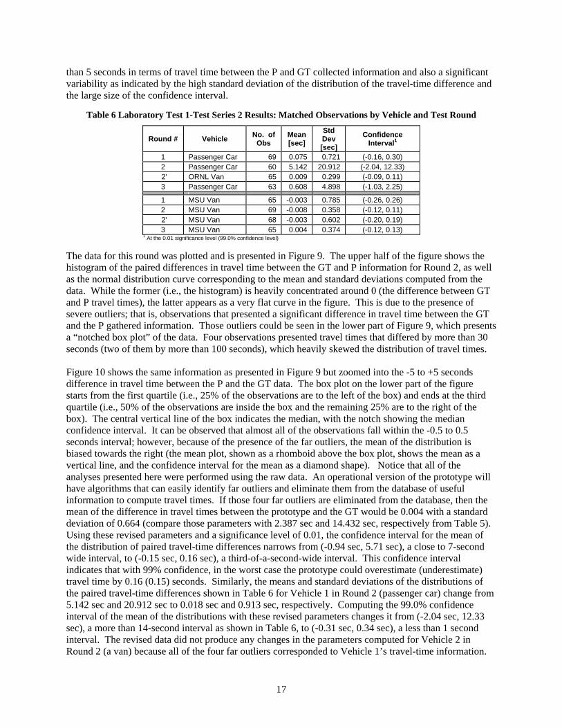
17

than 5 seconds in terms of travel time between the P and GT collected information and also a significant variability as indicated by the high standard deviation of the distribution of the travel-time difference and the large size of the confidence interval.

Table 6 Laboratory Test 1-Test Series 2 Results: Matched Observations by Vehicle and Test Round

Round # Vehicle No. of Obs

Mean [sec]

Std Dev [sec]


1 Passenger Car 69 0.075 0.721 (-0.16, 0.30) 2 Passenger Car 60 5.142 20.912 (-2.04, 12.33) 2' ORNL Van 65 0.009 0.299 (-0.09, 0.11) 3 Passenger Car 63 0.608 4.898 (-1.03, 2.25)

1 MSU Van 65 -0.003 0.785 (-0.26, 0.26) 2 MSU Van 69 -0.008 0.358 (-0.12, 0.11) 2' MSU Van 68 -0.003 0.602 (-0.20, 0.19) 3 MSU Van 65 0.004 0.374 (-0.12, 0.13)

1 At the 0.01 significance level (99.0% confidence level) The data for this round was plotted and is presented in Figure 9. The upper half of the figure shows the histogram of the paired differences in travel time between the GT and P information for Round 2, as well as the normal distribution curve corresponding to the mean and standard deviations computed from the data. While the former (i.e., the histogram) is heavily concentrated around 0 (the difference between GT and P travel times), the latter appears as a very flat curve in the figure. This is due to the presence of severe outliers; that is, observations that presented a significant difference in travel time between the GT and the P gathered information. Those outliers could be seen in the lower part of Figure 9, which presents a “notched box plot” of the data. Four observations presented travel times that differed by more than 30 seconds (two of them by more than 100 seconds), which heavily skewed the distribution of travel times. Figure 10 shows the same information as presented in Figure 9 but zoomed into the -5 to +5 seconds difference in travel time between the P and the GT data. The box plot on the lower part of the figure starts from the first quartile (i.e., 25% of the observations are to the left of the box) and ends at the third quartile (i.e., 50% of the observations are inside the box and the remaining 25% are to the right of the box). The central vertical line of the box indicates the median, with the notch showing the median confidence interval. It can be observed that almost all of the observations fall within the -0.5 to 0.5 seconds interval; however, because of the presence of the far outliers, the mean of the distribution is biased towards the right (the mean plot, shown as a rhomboid above the box plot, shows the mean as a vertical line, and the confidence interval for the mean as a diamond shape). Notice that all of the analyses presented here were performed using the raw data. An operational version of the prototype will have algorithms that can easily identify far outliers and eliminate them from the database of useful information to compute travel times. If those four far outliers are eliminated from the database, then the mean of the difference in travel times between the prototype and the GT would be 0.004 with a standard deviation of 0.664 (compare those parameters with 2.387 sec and 14.432 sec, respectively from Table 5). Using these revised parameters and a significance level of 0.01, the confidence interval for the mean of the distribution of paired travel-time differences narrows from (-0.94 sec, 5.71 sec), a close to 7-second wide interval, to (-0.15 sec, 0.16 sec), a third-of-a-second-wide interval. This confidence interval indicates that with 99% confidence, in the worst case the prototype could overestimate (underestimate) travel time by 0.16 (0.15) seconds. Similarly, the means and standard deviations of the distributions of the paired travel-time differences shown in Table 6 for Vehicle 1 in Round 2 (passenger car) change from 5.142 sec and 20.912 sec to 0.018 sec and 0.913 sec, respectively. Computing the 99.0% confidence interval of the mean of the distributions with these revised parameters changes it from (-2.04 sec, 12.33 sec), a more than 14-second interval as shown in Table 6, to (-0.31 sec, 0.34 sec), a less than 1 second interval. The revised data did not produce any changes in the parameters computed for Vehicle 2 in Round 2 (a van) because all of the four far outliers corresponded to Vehicle 1’s travel-time information.

18

Histogram

0

10

20

30

40

50

60

70

-30 -25 -20 -15 -10 -5 0 5 10 15 20 25 30 35 40 45 50 55 60 65 70 75 80 85 90 95 100 105 110 115 120Diff TT

Freq

uenc

y

Normal Fit(Mean=2.3874, SD=14.4324)

-30 -25 -20 -15 -10 -5 0 5 10 15 20 25 30 35 40 45 50 55 60 65 70 75 80 85 90 95 100 105 110 115 120Diff TT

95% CI Notched Outlier BoxplotMedian (0.0120)

95% CI Mean DiamondMean (2.3874)

Outliers > 1.5 and < 3 IQR

Outliers > 3 IQR

Figure 9 Laboratory Test 1 Round 2 Travel Time Differences Frequency Distribution (GT and P Paired Data) - Histogram and Box Plot (TT Diff in sec)

19

Histogram

0

5

10

15

20

25

30

35

40

45

-5.00 -4.50 -4.00 -3.50 -3.00 -2.50 -2.00 -1.50 -1.00 -0.50 0.00 0.50 1.00 1.50 2.00 2.50 3.00 3.50 4.00 4.50 5.00

Diff TT

Freq

uenc

yNormal Fit(Mean=2.3874, SD=14.4324)

-5.00 -4.50 -4.00 -3.50 -3.00 -2.50 -2.00 -1.50 -1.00 -0.50 0.00 0.50 1.00 1.50 2.00 2.50 3.00 3.50 4.00 4.50 5.00Diff TT




Outliers > 3 IQR

Figure 10 Laboratory Test 1 Round 2 Travel Time Differences Frequency Distribution (GT and P Paired Data) - Histogram and Box Plot (Zoomed around the Mean of the Distribution of TT Diff; TT Diff in sec)

The histograms and box plots of the revised (i.e., no extreme far outliers) travel-time difference distribution is presented in Figure 11. Notice that there are still some observations (four) that could qualify as far outliers. Those observations could be easily identified by any filtering algorithm and eliminated from the database, thus further reducing the variance of the differences in travel time between the prototype and the GT-gathered information.

Histogram

0

5

10

15

20

25

30

35

40

45

-4.00 -3.50 -3.00 -2.50 -2.00 -1.50 -1.00 -0.50 0.00 0.50 1.00 1.50 2.00 2.50 3.00 3.50 4.00Diff TT

Freq

uenc

y


-4 -3.5 -3 -2.5 -2 -1.5 -1 -0.5 0 0.5 1 1.5 2 2.5 3 3.5 4

Diff TT

95% CI Notched Outlier BoxplotMedian (-0.013)



Outliers > 3 IQR

Figure 11 Laboratory Test 1 Revised Round 2 Travel Time Differences Frequency Distribution (GT and P Paired Data) - Histogram and Box Plot, Excluding Four Far Outliers (TT Diff in sec)

The information presented graphically in Figure 11 is also shown numerically in Table 7. Several summary statistics are also presented in that table. The mean and median of the distribution of travel-time differences are presented with their corresponding 99% confidence intervals. The coefficient SE (standard error) expresses the variability of the mean, which in this case is very small. The skewness

20

coefficient is a measure of the asymmetry of the probability distribution of the distribution of travel-time differences. A positive skew, as is the case of Round 2, signifies that the right tail of the distribution is longer than the left tail, indicating an overestimation of travel time by the prototype. The high Kurtosis coefficient4 (greater than 3) indicates in this case that more of the variance is due to infrequent extreme deviations (e.g., those far outliers identified earlier), as opposed to frequent modestly-sized deviations. The Shapiro-Wilk Test tests the null hypothesis that the sample of travel-time differences came from a normally distributed population, which in this case can be rejected at a 99.99% confidence level (i.e., p<0.0001). Again, this is mostly due to the presence of the far outliers, which in an operational system can be easily identified and eliminated from the database. The interquartile range (IQR) is a measure of statistical dispersion; and is equal to the difference between the third and first quartiles of the travel time distribution (presented in Table 7 under the “Percentile” header). This measure, which is very low for the distribution under consideration, indicates that 50% of the observations presented a difference in travel time between the GT and P information that was less than 0.388 seconds.

Table 7 Laboratory Test 1-Revised Round 2 Travel Time Differences Distribution Summary Statistics

(GT and P Paired Data)

n 125

Mean 0.004 Median -0.013 99% CI -0.151 to 0.159 95.% CI -0.077 to 0.058

SE 0.059

Variance 0.440 Range 6.74 SD 0.664 IQR 0.388

99% CI 0.570 to 0.791

Skewness 0.38 Percentile Kurtosis 17.18 0th -3.345 (minimum)

25th -0.203 (1st quartile) Shapiro-Wilk W 0.64 50th -0.013 (median)

p <0.0001 75th 0.185 (3rd quartile) 100th 3.396 (maximum)

TT Differences Statistics in sec.

Other data collected in these tests included sensor setup times, but did not include loop detector deployment times (because this phase of the project focused on the detection accuracy and the reliability of the sensors and communication system). During the first day of this laboratory test series, the deployment and connection of the sensors required about 20-25 minutes for each box. These long deployment/connection times were mostly due to the fact that this was the first time that the prototype sensors were deployed and several technical issues had to be resolved. During the second day, those times were reduced to about 10-15 minutes. After the first test series was concluded, IST returned the sensors to their laboratory for further adjustments and corrections. 2.2.1.3 Test Conclusions The main goals of the first laboratory tests were to determine the reliability of the system, to investigate the ability of the sensors to differentiate among different vehicles, and to determine the accuracy of the prototype system in estimating travel time between sensors. The reliability of the system was defined as the percentage of times that the prototype system was able to make a successful identification of a given

4 The Kurtosis coefficient is a measure of the "peakedness" of the probability distribution.

21

vehicle at two different sensors. Accuracy was computed by dividing the absolute difference of the means of the GT and P travel-time distributions by the mean of the former, and subtracting that number from one. Test Series 1 involved only one vehicle and therefore it was possible to determine the highest achievable reliability of the system composed by three sensors. This parameter was estimated at 97.75% under the testing conditions. It was not 100% (as it could theoretically be expected when there is only one vehicle involved) due to issues such as the vehicle crossing one of the loop detectors at an angle that is significantly different from a 90-degree angle (i.e., a non-perpendicular direction of travel with respect to the loop detectors). Such as crossing creates a different inductive signature which could impede the re-identification of the vehicle. The accuracy of the system was measured at 99.71%. In Test Series 2, two vehicles were used. In some of the rounds, the vehicles were very similar to one another (two vans), and in others they were different (a van and a passenger car). In one of the rounds involving two different vehicles, the prototype produced four observations (travel times) that were far outliers (i.e., travel time ranging from 40 to more than 100 seconds, when the average travel time was less than 20 seconds). Once these observations were eliminated from the database, the system presented a reliability that was above 92%, and accuracy levels that were above 95%. In all cases, and once the severe outliers were eliminated for Round 2, the null hypothesis Ho stating that the means of the travel-time distributions generated with the GT and P data were the same could only be rejected at a very low confidence level (less than 50%), thus concluding that both travel-time means were the same. 2.2.2 Second Laboratory Test Series (NTRC, December 2007) 2.2.2.1 Test Description The second series of controlled tests were conducted at the NTRC main parking lot on December 15th and 16th, 2007. The tests consisted of deploying the three prototype sensors with their corresponding communication and power supply hardware as indicated in Figure 12, with two, and in some cases three, vehicles traveling over the loop detectors to generate traffic information. Travel-time information was also measured exogenously to the system by means of stopwatches which were used to record the time it took to travel from one sensor to the next as described in the previous section [see First Laboratory Test Series (NTRC, November 2007)].

Objectives of the Test. As in the case of the first laboratory tests, a main objective of the test was to investigate the ability of the sensors to differentiate among different vehicles, but this time under increasing stochastic travel patterns. This second test had an additional objective, which was to determine the sensitivity of the system to the geometry and the anchoring of the loop detectors. To accomplish this second objective, a set of loop detectors was built by ORNL taping the wires to flat plastic strips measuring about 5 feet in length by 1 inch wide; with four of these strips forming each one of the two loops required by each controller. The wire was only taped at six points on each one of the plastic strips, and those plastic strips were in turn taped to the pavement forming loop detectors (i.e., two rectangles of 11 feet by 4 feet separated by 1 foot, with the longer dimension perpendicular to the direction of travel) that the sensors used during this laboratory test. Because the wires were not firmly anchored to the pavement, they would move while traffic was traveling on top of the loop detectors, thus generating noise in the inductive signature that is used to identify the vehicles. This situation would be representative of a real-world case (emergency evacuation) in which the sensors, because of time constraints, are placed on the pavement without any caution. That is, this second test was trying to determine how much degradation in the system would be introduced by placing the sensors in the worst manner possible. The

22

degradation of the system was determined by measuring its reliability and accuracy under the testing conditions.

S0

S1S2

Figure 12 Sensor Setup at the NTRC Main Parking Lot (Second Laboratory Test)

Test Series 1 Setup and Procedures. For this test series, two test vehicles were used (two vans of different makes) which followed a specific travel pattern. Both vehicles circled the parking lot following a counter-clockwise direction as indicated in Figure 12 and always drove over the three loop detectors. However, the vehicles did not follow one another, but rather one overtook another in a random fashion in order to create stochastic traffic patterns that would increase the level of difficulty for the system to generate travel times in each segment. The order in which each vehicle crossed any given sensor in each run of this test series is presented in Table 8. Consider, for example, Run 10. For this run the random order pattern indicated that Veh1 should travel over Sensor 0 (see Figure 12) first followed by Veh2; then Veh2 should travel over Sensor 1 ahead of Veh1; and finally, Veh1 should overtake Veh2 and drive first over Sensor 2. Besides following the sensor-crossing patterns indicated in Table 8, each vehicle selected a given speed on each segment (adding delays in a random fashion) such that the travel time in each segment was not a constant quantity. Before the test started, two stopwatches, SW1 and SW2, one for each vehicle were synchronized and started at a given time (obtained from a cell phone). The stopwatches were stopped every time a vehicle went over a given sensor and the readings were noted and used to determine GT travel times. Objectives of Test Series 1. To investigate the ability of the sensors to differentiate among similar vehicles and to determine the prototype’s ability to estimate the travel time between sensors under extremely poor deployment conditions.

23

Test Series 2 Setup and Procedures. The second test series consisted of three additional rounds where the two vehicles were driven following a given travel pattern that was randomly selected before the test. The three patterns used were the same as those used in the November 2007 tests (see First Laboratory Test Series (NTRC, November 2007)). Test Pattern 1 (TP1). This pattern was similar to that of Test Series 1. The test vehicle traveled over Sensor S0 (the elapsed time was noted), turned around, followed the direction of travel indicated in Figure 12, drove over Sensor S1 (the elapsed time was noted) and continued traveling in a counter-clockwise direction to drive over Sensor S2 (the elapsed time was noted). Test Pattern 2 (TP2). This travel pattern was similar to TP1 except that the test vehicle avoided Sensor S1. For Rounds 2 and 3, the vehicle stopped for a given number of seconds (randomly selected prior to the test) before going to Sensor 2 in order to add delays to the travel time of that segment (i.e., Segment S0-S2) thus increasing the stochasticity of this variable. Test Pattern 3 (TP3). This travel pattern was similar to TP1 except that the test vehicle avoided Sensor S2. Random segment delays were also added to this pattern in Rounds 2 and 3.

Table 8 Sensor Crossing Order for Veh1 and Veh2

Sensor 0 Sensor 1 Sensor 2 Run # Veh1

Drives Veh2

Drives Veh1

Drives Veh2

Drives Veh1

Drives Veh2

Drives 1 2nd 1st 2nd 1st 2nd 1st 2 1st 2nd 1st 2nd 2nd 1st 3 1st 2nd 2nd 1st 1st 2nd 4 1st 2nd 2nd 1st 2nd 1st 5 2nd 1st 1st 2nd 2nd 1st 6 1st 2nd 2nd 1st 2nd 1st 7 2nd 1st 1st 2nd 2nd 1st 8 1st 2nd 1st 2nd 2nd 1st 9 2nd 1st 1st 2nd 2nd 1st

10 1st 2nd 2nd 1st 1st 2nd 11 2nd 1st 1st 2nd 1st 2nd 12 1st 2nd 1st 2nd 1st 2nd 13 2nd 1st 2nd 1st 1st 2nd 14 2nd 1st 1st 2nd 2nd 1st 15 1st 2nd 1st 2nd 2nd 1st 16 2nd 1st 1st 2nd 1st 2nd 17 2nd 1st 1st 2nd 1st 2nd 18 2nd 1st 2nd 1st 1st 2nd 19 2nd 1st 1st 2nd 2nd 1st 20 1st 2nd 1st 2nd 2nd 1st 21 2nd 1st 1st 2nd 1st 2nd 22 2nd 1st 2nd 1st 1st 2nd 23 2nd 1st 1st 2nd 2nd 1st 24 1st 2nd 2nd 1st 2nd 1st 25 1st 2nd 2nd 1st 2nd 1st 26 2nd 1st 1st 2nd 2nd 1st 27 1st 2nd 1st 2nd 2nd 1st 28 2nd 1st 1st 2nd 2nd 1st 29 1st 2nd 2nd 1st 2nd 1st 30 1st 2nd 2nd 1st 2nd 1st

The travel patterns for Veh1 and Veh2 were assigned at random and are presented in Table 9 (note: in Round 3, a passenger car was used instead of the van Veh2 for Runs 8 to 11 to add another level of

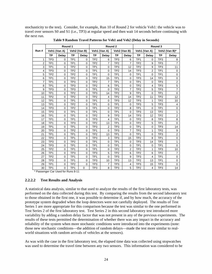
24

stochasticity to the test). Consider, for example, Run 10 of Round 2 for vehicle Veh1: the vehicle was to travel over sensors S0 and S1 (i.e., TP3) at regular speed and then wait 14 seconds before continuing with the next run.

Table 9 Random Travel Patterns for Veh1 and Veh2 (Delay in Seconds)

Round 1 Round 2 Round 3 Veh1 (Van A) Veh2 (Van B) Veh1 (Van A) Veh2 (Van B) Veh1 (Van A) Veh2 (Van B)* Run # TP Delay TP Delay TP Delay TP Delay TP Delay TP Delay

1 TP3 0 TP1 0 TP2 6 TP3 6 TP1 0 TP3 8 2 TP1 0 TP1 0 TP2 7 TP2 7 TP2 9 TP3 7 3 TP1 0 TP2 0 TP1 0 TP3 12 TP2 9 TP3 11 4 TP3 0 TP2 0 TP1 0 TP2 14 TP3 2 TP1 0 5 TP2 0 TP2 0 TP1 0 TP1 0 TP1 0 TP1 0 6 TP1 0 TP2 0 TP2 15 TP1 0 TP3 14 TP1 0 7 TP1 0 TP3 0 TP2 7 TP1 0 TP1 0 TP3 2 8 TP1 0 TP3 0 TP2 6 TP1 0 TP2 4 TP3 5 9 TP3 0 TP3 0 TP1 0 TP2 7 TP2 5 TP3 7

10 TP1 0 TP2 0 TP3 14 TP2 9 TP1 0 TP1 0 11 TP2 0 TP2 0 TP2 4 TP2 14 TP2 11 TP2 12 12 TP1 0 TP1 0 TP1 0 TP3 12 TP3 1 TP2 10 13 TP1 0 TP2 0 TP1 0 TP1 0 TP3 5 TP3 4 14 TP3 0 TP2 0 TP1 0 TP2 8 TP1 0 TP1 0 15 TP3 0 TP1 0 TP1 0 TP1 0 TP3 13 TP2 1 16 TP1 0 TP1 0 TP2 9 TP3 14 TP3 12 TP2 2 17 TP1 0 TP1 0 TP3 4 TP1 0 TP2 8 TP3 8 18 TP1 0 TP3 0 TP2 13 TP1 0 TP2 5 TP1 0 19 TP1 0 TP1 0 TP3 2 TP3 0 TP1 0 TP3 14 20 TP3 0 TP2 0 TP1 0 TP3 7 TP2 1 TP2 9 21 TP1 0 TP1 0 TP2 13 TP1 0 TP1 0 TP3 2 22 TP3 0 TP1 0 TP3 3 TP3 15 TP2 8 TP1 0 23 TP3 0 TP2 0 TP1 0 TP1 0 TP3 14 TP3 1 24 TP3 0 TP1 0 TP1 0 TP1 0 TP1 0 TP1 0 25 TP2 0 TP1 0 TP1 0 TP2 2 TP2 1 TP3 10 26 TP1 0 TP3 0 TP3 5 TP2 6 TP2 6 TP2 7 27 TP2 0 TP1 0 TP1 0 TP3 9 TP3 4 TP1 0 28 TP3 0 TP1 0 TP3 10 TP3 13 TP2 13 TP1 0 29 TP1 0 TP2 0 TP3 7 TP3 4 TP3 15 TP3 0 30 TP1 0 TP1 0 TP3 8 TP3 5 TP2 4 TP3 14

* Passenger Car Used for Runs 8-11 2.2.2.2 Test Results and Analysis A statistical data analysis, similar to that used to analyze the results of the first laboratory tests, was performed on the data collected during this test. By comparing the results from the second laboratory test to those obtained in the first one, it was possible to determine if, and by how much, the accuracy of the prototype system degraded when the loop detectors were not carefully deployed. The results of Test Series 1 are more appropriate for this comparison because the test was similar to the one performed in Test Series 2 of the first laboratory test. Test Series 2 in this second laboratory test introduced more variability by adding a random delay factor that was not present in any of the previous experiments. The results of these tests permitted the determination of whether there was any impact in the accuracy and reliability of the system when more stochastic conditions were introduced into the experiments (note: those new stochastic conditions—the addition of random delays—made the test more similar to real-world situations with random arrivals of vehicles at the sensors). As was with the case in the first laboratory test, the elapsed time data was collected using stopwatches was used to determine the travel time between any two sensors. This information was considered to be

25

the GT for the comparisons with the data provided by the sensors. Notice that this GT data is not error free because it was manually collected (i.e., the operator was attempting to stop the stopwatch at the same location when the vehicle was passing over each of the loop detectors); however, these human errors were very likely randomly distributed and should not have affected the results significantly. With the large size of data (over 180 observations) in each round, the errors might be canceled out by themselves. Test Series 1. As explained above, this experiment was designed to determine the ability of the system to produce results under extremely degraded deployment conditions (i.e., loop wires that had large relative movements respective to one another; introducing significant noise in the inductive signals generated by the vehicles). After the system was deployed, ORNL researchers checked that each sensor was communicating with a central website that was created for the purpose of displaying sensor information in real time. Through the website it was possible to see at when each sensor was turned on or off, however, the communication system did not send any traffic information collected in the field. Because it was unfeasible to fix this problem at that time, the test went ahead as described above. The data collected was stored at each one of the sensor’s computers. After the test was concluded and once the data was retrieved, it was apparent that Sensor S0 had a malfunction and did not record any information. As a result, information collected and was analyzed on just one of the three segments (i.e., Segment S1-S2). The test results are summarized in Table 10. The first row of the table shows the results of Test Series 1. A total of 180 data points (i.e., travel times between two sensors) were collected using two vans of different makers as the test vehicles; 54 of those one-hundred-eighty observations corresponded to Segment S1-S2. For that segment, the prototype system was able to identify/re-identify the vehicles in thirty occasions, which gives the system a reliability of 55.6% under the testing conditions. This reliability level was considered low for a controlled experiment and was further investigated by analyzing each vehicle separately as discussed below (see the Test Series 2 discussion). The table also shows the average and standard deviations of the distributions of travel times computed with the GT data and the information provided by the prototype system. The means of the P and GT travel-time distributions were used to compute the accuracy of the prototype system in assessing travel time, which was determined to be 98.5%—i.e., 100-Abs(26.03-25.64)/25.64*100.

Table 10 Laboratory Test 2 Results: All Data by Test Series and Test Round

GT Prototype Test

Series Round

# Total Obs.

S1-S21 Obs.

Mean [sec]

Std Dev [sec]

S1-S2 Obs.

Mean [sec]

Std Dev [sec]

No. of Mismatches2

Reliability [%]

Accuracy [%]

Reject Ho

3 at [%]

1 1 180 54 25.64 5.19 52 26.03 4.06 24 55.56 98.47 <50.00

1 146 27 21.22 3.11 32 21.13 1.38 13 51.85 99.60 91.732 142 24 21.42 2.61 28 22.18 1.84 14 41.67 96.45 96.422

34 136 18 21.98 2.30 24 22.72 1.64 8 55.56 96.61 96.75 1 Observations that were too low (e.g., 0.9 sec) were eliminated: 6 in Test Series 1 Round 1 and 1 in Test Series 2 Round 1. All corresponded to vehicle 1 (MSU van).

2 Includes as a mismatch only cases where GT travel time existed and P travel time did not. 3 Ho: The means of the GT and P travel-time distributions are the same. 4 For four of the runs, a passenger car was used instead of vehicle 2 (the ORNL van)

The mean and standard deviations of the P and GT travel-time distributions were also used to test the null hypothesis (Ho) that the averages of both the GT and P travel-time distributions were the same, against the alternative hypothesis (Ha) that they were different. A t-test was used to determine the confidence level at which the null hypothesis could be rejected. This value, which is presented in the last column of Table 10, indicates that for Test Series 1, Ho could only be rejected with a very low confidence level, thus indicating that both travel-time means are the same.

26

Consider now, Table 11; the first row in the table presents additional information for Test Series 1. Using only the matched information (i.e., those runs in which the prototype produced readings in which the arrival time at the downstream sensor of a giving segment was the same as that generated by the GT data collection procedures), columns 6 and 7 in Table 11 present the mean and standard deviation of the distribution of the difference in travel time between the P and the GT information (paired data). The last column of the table presents the confidence interval for the mean of the distribution at a significance level of 0.01 (i.e., confidence level of 99.0%), which for Round 1 was between -0.13 and 0.29 seconds. That is, with 99% confidence, the prototype could overestimate travel time by no more than 1/3 second on average (or underestimate it by no more than 1/6 second) for an average travel time of about 26 seconds.

Table 11 Laboratory Test 2 Results: Matched Observations by Test Series and Test Round

Test Series

Round # Veh1 Veh2 No. of

Obs Mean [sec]

Std Dev [sec]


1 1 MSU Van ORNL Van 30 0.079 0.413 (-0.13 , 0.29)

1 MSU Van ORNL Van 14 0.070 0.101 (-0.01 , 0.15) 2 MSU Van ORNL Van 10 0.104 0.131 (-0.03 , 0.24) 2 32 MSU Van ORNL Van 10 0.147 0.203 (-0.06 , 0.36)

1 At the 0.01 significance level (99.0% confidence level). 2 For four of the runs, a passenger car was used instead of the ORNL Van.

Test Series 2. The results of the data analysis for Test Series 2 are presented in Table 10 through Table 12. Using all of the data collected during the test, Table 10 shows some general information such as the number of observations (i.e., the travel times measured by both the operators conducting the tests and the prototype system) for all the segments, and the averages and standard deviations of the travel-time distributions obtained with information collected by the prototype and from the GT data for Segment S1-S2. During this test series, the reliability of the system ranged from 42% to 56%. This reliability level was considered low for a controlled experiment and was further investigated by analyzing each vehicle separately as discussed below. The prototype system achieved a level of accuracy that was above 96% in all cases. Similarly to the Test Series 1 case, the null hypothesis Ho stating that the means of the travel-time distributions generated with the GT and P data were the same, was tested for Series 2. The results of the tests indicated that except for Round 1, Ho could be rejected with more than a 95% confidence level (i.e., the typical statistical rejection limit), thus suggesting that the means of the travel-time distributions generated with the GT and P data were different when all of the data collected was used in the analysis. However, when only the matches between the prototype and GT were used in the analysis (see Table 11), the travel time provided by the prototype in all three rounds of Test Series 2 presented, on average, an error of less than 0.5second. Notice that, as discussed previously, a “match” refers to the condition in which both GT and the P register the same (or almost the same) arrival time at the downstream sensor of any given segment. Notice also that this does not imply that the travel times for that segment are the same for the GT and P (i.e., they could be different because of misidentifications upstream, thus indicating the presence of an error in determining the P travel time). These results clearly indicated that the mismatches, which were significantly higher in this second laboratory test, played an important role in defining the distribution of travel times, which even though they presented a mean that was very close to the GT mean (as indicated by the accuracy parameter), it was different from the one generated by the GT observations (as indicated by the high confidence in rejecting Ho). Those results, therefore, warranted a more in-depth analysis of the information collected. Table 12 shows the results of the four rounds of tests disaggregated by vehicle. It is clear that in all of them the prototype system had problems identifying/re-identifying Vehicle 1 (the MSU van). In fact, in all the rounds of Test Series 2, Vehicle 1 was never re-identified, and, in Series 1, it was identified only

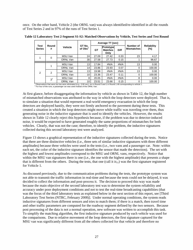
27

once. On the other hand, Vehicle 2 (the ORNL van) was always identified/re-identified in all the rounds of Test Series 2 and in 97% of the runs of Test Series 1.

Table 12 Laboratory Test 2-Segment S1-S2: Matched Observations by Vehicle, Test Series and Test Round

Average TT [sec] Test

Series Round

# Vehicle GT No. of Obs1 GT

Prototype Matches

Only Diff

Number of Mismatches

Reliability [%]

MSU Van 24 27.09 27.42 0.33 23 4.17 1 0 ORNL Van 30 27.58 27.73 0.15 1 96.67

MSU Van 13 17.84 #N/A #N/A 13 0.00 1 ORNL Van 14 23.86 23.93 0.07 0 100.00 MSU Van 13 19.98 #N/A #N/A 13 0.00 2

ORNL Van 10 23.36 23.47 0.11 0 100.00 MSU Van 8 20.05 #N/A #N/A 8 0.00

2

32 ORNL Van 10 23.51 23.66 0.15 0 100.00

1 Observations that were too low were eliminated (e.g., 0.90 sec), six in Round 0 and 1 in Round 1 All corresponding to vehicle 1. 2 For four of the runs, a passenger car was used instead of the ORNL Van.

At first glance, before disaggregating the information by vehicle as shown in Table 12, the high number of mismatched observations was attributed to the way in which the loop detectors were deployed. That is, to simulate a situation that would represent a real-world emergency evacuation in which the loop detectors are deployed hastily, they were not firmly anchored to the pavement during these tests. This created a situation in which the loop detectors might move while traffic was traveling over them, thus generating noise in the inductive signature that is used to identify the vehicles. However, the results shown in Table 12 clearly reject this hypothesis because, if the problem was due to detector-induced noise, it would be expected to have generated roughly the same proportions of mismatches for both vehicles. Clearly, that was not the case; therefore, to identify the problem, the inductive signatures collected during this second laboratory test were analyzed. Figure 13 shows a graphical representation of the inductive signatures collected during the tests. Notice that there are three distinctive vehicles (i.e., three sets of similar inductive signatures with three different amplitudes) because three vehicles were used in the tests (i.e., two vans and a passenger car. Note: within each set, the color of the inductive signature identifies the sensor that made the detection). The set with the highest and lowest amplitudes correspond to the MSU and ORNL vans, respectively. Notice that within the MSU van signatures there is one (i.e., the one with the highest amplitude) that presents a shape that is different from the others. During the tests, that one (call it is11) was the first signature registered for Vehicle 1. As discussed previously, due to the communication problems during the tests, the prototype system was not able to transmit the traffic information in real-time and because the tests could not be delayed, it was decided to collect the information and post-process it. The decision to proceed this way was made because the main objective of the second laboratory test was to determine the system reliability and accuracy under poor deployment conditions and not to test the real-time broadcasting capabilities (that was the focus of the third laboratory tests as explained below in the next section of this report, see [Third Laboratory Test Series (NTRC, February 2008)]. Under normal operating conditions, the system reads inductive signatures from different sensors and tries to match them; if there is a match, then travel time and other traffic parameters are computed for the roadway segment defined by the two sensors. Because post processing of the data is not a normal operation, new software was written to accomplish this task. To simplify the matching algorithm, the first inductive signature produced by each vehicle was used for the comparisons. Due to relative movement of the loop detectors, the first signature captured for the MSU van was significantly different from all the others collected for that vehicle and therefore no

28

subsequent matches were observed. Under normal operations, this first signature would have not been matched and therefore would have been discarded by the system. The inductive signatures that were collected afterwards would have been matched because they are very similar (see Figure 13) and the system would have presented a reliability level for the MSU van similar to that obtained for the ORNL van and the passenger car.

Figure 13 Inductive Signatures Captured by the Prototype Sensors during the 2nd Laboratory Test

The problem described was only identified during the analysis of the data when the information collected was disaggregated by vehicle. Because the graphical representation of the inductive signatures suggested that a high matching rate would have been obtained for the MSU van, no re-processing of the data (which would have implied rewriting the post-processing software) was performed. As an illustration of how the P and GT matched data compares, Figure 14 shows a graph of travel time for Round 1 of Series 1 (note: the three rounds of Test Series 2 showed similar results as those presented here). The figure shows two graphs for the travel time provided by the prototype. The travel times are vertically displaced by a constant quantity (i.e., 5.4 seconds) with the raw data showing smaller travel times. The reason for this was that the internal clock of the computer at Sensor S2 was off by 5.4 seconds. That is, when a vehicle crossed that sensor, its inductive signature was time stamped with a label that showed a time that was 5.4 seconds earlier than what it should have been, thus generating travel times that were 5.4 seconds shorter. The synchronization of the internal clocks of the sensor computers is an issue that could potentially introduce errors in the computations of travel times, as was the case in this laboratory test. This issue, however, could be easily resolved by using the time gathered by the on-board GPS device to correct the internal clock of these computers. Because all of the GPS devices get the same (universal) time, the internal clocks used by the sensors to timestamp the collected inductive signatures were synchronized.

29

Once the synchronization problem was resolved, the P showed travel times were almost identical to the GT travel times. Notice that for one of the observations (the one inside the circle in Figure 14) there was a discrepancy between the P and the GT that was larger than for any other observation. This particular point was the only match of the MSU van and could have been merely an anomaly.

0.00

5.00

10.00

15.00

20.00

25.00

30.00

35.00

40.00

48000 48500 49000 49500 50000 50500 51000

Elapsed Time [sec since Midnight]

Trav

el T

ime

[sec

]

GT P P (Raw)

Figure 14 Prototype and “Ground-Truth” Travel Time Information

(Second Laboratory Test Series 1 – Round 1 – Segment S1-S2) The information presented in the figure above is summarized in Table 13, which shows the mean difference between paired travel-time observations to be 0.079 seconds (i.e., on average, the P system overestimated travel time by less than 0.10 of a second). The table also shows that the tests of hypothesis that the mean of the GT and P distributions for the matched data were the same could only be rejected at a very low confidence level. The three rounds of Test Series 2 showed similar results as those of Series 1.

Table 13 Travel Time Differences Distribution Summary Statistics (GT and P Paired Data for Test Series 1 – Round 1)

n 60

Groups n Mean SE SD GT TT 30 27.56 0.613 3.36

P TT 30 27.65 0.610 3.34

Mean difference 0.079 99% CI -0.13 to 0.29

SE 0.08

t statistic 1.05 DF 29.0

2-tailed p 0.3071 Reject Ho at 69.29% Confidence Level


30

2.2.2.3 Test Conclusions The main goal of the second laboratory tests was to investigate the ability of the sensors to differentiate among different vehicles under increasing stochastic travel patterns. The stochasticity of the tests was increased, when compared with Laboratory Test 1, by introducing random vehicle-following patterns (i.e., the vehicles crossed the upstream and downstream sensors in specific patterns that indicated when a vehicle had to overtake the other while traveling between any two sensors) and by adding random delays (i.e., the vehicles stopped for a random amount of time between the upstream and downstream sensors of any given segment). This second test had an additional objective, which was to assess the sensitivity of the system to the geometry and anchoring of the loop detectors, which was determined by measuring its reliability and accuracy under the testing conditions. In order to achieve conditions resembling a real-world case (emergency evacuation) in which the sensors, because of time constraints, are placed on the pavement without any caution, the wires were not firmly anchored to the pavement but rather attached to plastic strips that were taped to the road at few points. Three vehicles were used for the tests, two vans one of which was substituted for a passenger car in a few runs. When the results of the tests were analyzed in an aggregated form, the P system presented a low reliability (between 42% and 56%). This suggested that a “bad” deployment of the loop detectors could have a significant impact on the ability of the system in identifying and re-identifying vehicles (e.g., during Laboratory Test 1, in which the loop detectors were carefully taped to the pavement, the reliability of the system was between 84% and 99%). However, when the results were disaggregated by vehicle, it was observed that in almost 100% of the observations the system failed to identify/re-identify one of the vans (the MSU van) while the other vehicle (i.e., the ORNL van or the passenger car) was always identified/re-identified. A subsequent analysis showed that this problem was due to a glitch in the software that was used to post-process the information. Visual analysis of the collected inductive signatures indicated that under normal operations (i.e., real-time identification/re-identification of vehicles) this would not have happened and that the system would have presented a high reliability, even with loop detectors that were not perfectly anchored to the pavement.

2.2.3 Third Laboratory Test Series (NTRC, February 2008) 2.2.3.1 Test Description The third and final laboratory test was conducted at the NTRC parking lot on February 23rd, 2008. The tests consisted of deploying the three prototype sensors with their corresponding communication and power supply hardware as indicated in Figure 15, with two vehicles traveling by the prototype sensors to generate traffic information. Travel-time information was also measured exogenously to the system by means of stopwatches as it was done in the previous two laboratory tests (see First Laboratory Test Series (NTRC, November 2007) and Second Laboratory Test Series (NTRC, December 2007)).

Objectives of the Test. The main goal of the test was to assess the ability of the system to report the location of each sensor to a website and also to provide traffic information and display it in real time.

Test Setup and Procedures. For this test series, two test vehicles were used (two passenger cars of different makers) which followed a specific travel pattern. Both vehicles circled the parking lot following a counter-clockwise direction as indicated in Figure 15 and always drove over the three loop detectors.

31

Three rounds were conducted, each one of them consisting of thirty runs (i.e., thirty laps). For each run, the vehicles were assigned, at random, one of three different travel patterns and also a time delay (i.e., a stopping time). These three travel patterns were as follows: Test pattern 1 (TP1). The test vehicle traveled over Sensor S0 (the elapsed time was noted), drove by Sensor S1 (the elapsed time was noted) and continued traveling in a counter-clockwise direction to drive by Sensor S2 (the elapsed time was noted). Test pattern 2 (TP2). This travel pattern was similar to TP1, except that the test vehicle avoided Sensor S1. Test pattern 3 (TP3). This travel pattern was similar to TP1, except that the test vehicle avoided Sensor S2.

S0

S1S2

Figure 15 Sensor Setup at the NTRC Main Parking Lot (Third Laboratory Test)

The randomly assigned travel patterns followed in this test are presented in Table 14. Consider, for example, Run 1 of Round 3 for Vehicle 2. The vehicle was to travel over Sensors S0 and S1 (i.e., TP3) at regular speed and then wait 8 seconds before continuing with the next run. In the second run, Vehicle 2 had to repeat TP3 and wait for 14 seconds before proceeding to Run 3. Before the test started, two stopwatches, SW1 and SW2, one for each vehicle were synchronized and started at a given time (obtained from a cell phone). The stopwatches were stopped every time a vehicle went over a given sensor and the readings were noted. Those readings were later used to determine GT travel times.

32

Table 14 Random Travel Patterns for Veh1 and Veh2 (Delay in Seconds)

Round 1 Round 2 Round 3 Veh1 (PC A) Veh2 (PC B) Veh1 (PC A) Veh2 (PC B) Veh1 (PC A) Veh2 (PC B) Run # TP Delay

[sec] TP Delay [sec] TP Delay

[sec] TP Delay [sec] TP Delay

[sec] TP Delay [sec]

1 TP2 0 TP3 0 TP3 13 TP3 0 TP2 5 TP3 8 2 TP2 0 TP1 0 TP3 7 TP3 1 TP2 8 TP3 14 3 TP1 0 TP1 0 TP1 0 TP2 4 TP1 0 TP1 0 4 TP3 0 TP2 0 TP3 6 TP1 0 TP3 5 TP3 12 5 TP3 0 TP2 0 TP2 8 TP1 0 TP3 7 TP1 0 6 TP3 0 TP3 0 TP1 0 TP1 0 TP2 5 TP2 7 7 TP2 0 TP1 0 TP3 12 TP3 8 TP1 0 TP1 0 8 TP2 0 TP2 0 TP3 10 TP3 14 TP3 1 TP3 2 9 TP3 0 TP3 0 TP1 0 TP3 12 TP1 0 TP1 0

10 TP1 0 TP3 0 TP3 14 TP3 7 TP2 6 TP3 7 11 TP2 0 TP2 0 TP1 0 TP3 8 TP3 5 TP3 12 12 TP2 0 TP3 0 TP1 0 TP1 0 TP3 2 TP2 3 13 TP2 0 TP3 0 TP2 10 TP1 0 TP3 1 TP1 0 14 TP1 0 TP3 0 TP2 5 TP1 0 TP3 4 TP3 8 15 TP1 0 TP1 0 TP2 4 TP3 5 TP3 3 TP1 0 16 TP3 0 TP2 0 TP3 0 TP2 7 TP3 5 TP1 0 17 TP3 0 TP2 0 TP3 11 TP2 14 TP2 7 TP3 6 18 TP1 0 TP3 0 TP2 0 TP2 8 TP2 0 TP3 6 19 TP3 0 TP3 0 TP1 0 TP3 11 TP2 3 TP2 8 20 TP2 0 TP1 0 TP3 8 TP3 13 TP1 0 TP3 1 21 TP1 0 TP3 0 TP2 2 TP2 2 TP2 6 TP2 10 22 TP1 0 TP3 0 TP1 0 TP2 5 TP2 0 TP1 0 23 TP2 0 TP2 0 TP3 15 TP1 0 TP3 14 TP3 1 24 TP2 0 TP1 0 TP1 0 TP2 9 TP1 0 TP2 9 25 TP3 0 TP3 0 TP1 0 TP3 14 TP2 9 TP1 0 26 TP1 0 TP1 0 TP2 5 TP2 11 TP3 13 TP2 2 27 TP3 0 TP3 0 TP3 10 TP1 0 TP2 3 TP2 10 28 TP2 0 TP2 0 TP3 14 TP2 12 TP3 14 TP3 11 29 TP1 0 TP2 0 TP2 1 TP1 0 TP1 0 TP2 2 30 TP3 0 TP2 0 TP1 0 TP3 5 TP2 14 TP3 12

2.2.3.2 Test Results and Analysis Before conducting the tests, a pre-test run was performed with one vehicle driven by an ORNL researcher while another researcher was inspecting the website to which the collected traffic information was to be sent in real time. The pre-test indicated that the sensors reported their position correctly. Figure 16 to Figure 18 show the location of the sensors using their real-time reported coordinates, which were displayed on maps that could be accessed at any time from the website set up for this test (refer also to Figure 15 which shows a schematic diagram of the position of the sensors).

33

Figure 16 Reported Spatial Location of Sensor 1


34


During the test, each one of the three prototype sensors reported traffic information to the website once every minute (or less), which was considered a very good temporal resolution. At the end of the tests, screen captures were made of the website displaying the data collected (see Figure 19 to Figure 21). Notice that the time axes (abscissa) on the graphs indicate Pacific Time rather than Eastern Time (where the NTRC is located). This was due to the fact that IST directed the real-time information through an existing Web server that was setup on the west coast as part of another traffic research project unrelated to this one. Nevertheless, each one of the three screen captures contains an inset with the computer clock to show that the data was collected in real time. The figures show the information collected during Round 1 of this laboratory test. Notice also that the vehicles always traveled by Sensor S0 (i.e., the three travel patterns require the vehicle to traverse Sensor S0) and that two extra runs were performed (pre-test runs). This information is displayed in the lower-right graph, which shows vehicle classification. Sixty-two identifications were made by Sensor S0, and all of them were passenger cars –vehicle type 2 in the Federal Highway Administration (FHWA) vehicle classification scheme, which is the one adopted for the project. The other graphs showed average speed (at the sensor), volume (in vehicles per hour), and occupancy (i.e., the percentage of the time a vehicle is over the loop detector).

35

Figure 19 Real-Time Traffic Data Collected by Sensor 1

36


37


38

2.2.3.3 Test Conclusions The main goal of the third and final laboratory test was to assess the ability of the system to report the location of each sensor to a website and also to provide traffic information and display it in real time. The test setup and methodology was similar to those used in Laboratory Tests 1 and 2. The results of the tests showed that each component (sensor) of the system was able to broadcast its position accurately and provide traffic information in real time to a website.

2.3 CONTROLLED TESTS SUMMARY AND CONCLUSIONS Three laboratory (i.e., controlled) environment series of tests were conducted during this phase of the project. The first two tests focused mainly on the determination of the parameters (i.e., accuracy and reliability) of the prototype system and on “debugging” the prototype data collection sub-system. The main objective of the third laboratory test was to assess the ability of the prototype system to communicate the data gathered in the field in real time, including travel time between pairs of sensors, as well as speed, volume and vehicle classification at each one of the prototype sensors. The main goals of the first laboratory tests were to determine the reliability of the system under controlled environment, to investigate the ability of the sensors to differentiate among different vehicles and to determine the accuracy of the prototype system in estimating travel time between sensors. Test Series 1 involved only one vehicle; therefore, it was possible to determine the maximum achievable reliability of the system composed by three sensors, which was estimated at 97.75% under the testing conditions. It was not 100% (as it could theoretically be expected when there is only one vehicle involved) due to issues, such as the vehicle crossing one of the loop detectors at an angle that is significantly different from a 90-degree angle (i.e., a non-perpendicular direction of travel with respect to the loop detectors), thus creating a different inductive signature that could impede the re-identification of the vehicle. The accuracy of the system was measured at 99.71%. For tests involving two vehicles, the system showed a reliability that was above 92% and accuracy levels above 95%. In all cases, the null hypothesis Ho, the means of the travel-time distributions generated with the GT and P data were the same, could only be rejected at a very low confidence level (less than 50%), thus indicating that both travel-time means were the same. The purpose of the second laboratory tests was to investigate the ability of the sensors to differentiate among different vehicles under travel patterns that presented a level of stochasticity higher than those used in the first laboratory tests. The stochasticity of the tests was increased by introducing vehicle following patterns and travel delays that were randomly assigned before the test. An additional objective of these second laboratory tests was to assess the sensitivity of the system to the geometry and anchoring of the loop detectors, which was determined by measuring its reliability and accuracy under the testing conditions. In order to achieve conditions resembling a real-world case (emergency evacuation) in which the sensors, because of time constraints, are placed on the pavement hastily, the wires were not firmly anchored to the pavement but rather attached to plastic strips that were taped to the road at few points. Three vehicles were used for the tests, two vans and a passenger car (note: one of the vans was substituted for the passenger car in a few runs). The results of the test indicated that the system presented a high reliability, even with loop detectors that were not perfectly anchored to the pavement. The third and final laboratory test showed that each component of the system (i.e., sensor) was able to broadcast its position accurately and provide traffic information in real time to a website.

39

After the three laboratory tests were completed, the prototype system was deemed ready to enter the next battery of tests in an environment closer to the one in which it will ultimately operate. Those tests are described in the following section.

40


41

3. FIELD OPERATION TESTS 3.1 INTRODUCTION During the first part of the project a battery of “laboratory environment” tests (i.e., tests that were conducted under highly controlled conditions) were performed with the main objective of identifying and correcting problems related to the different components of the prototype system. Preliminary data analyses of the information collected by the system was performed concurrently with the tests (i.e., the data was analyzed as it was gathered or immediately thereafter), which allowed making adjustments to both the data collection procedures and the prototype system itself. Any identified deficiencies in the prototype system were corrected expediently; subsequent tests were used to determine if the adjustments made to the prototype had been successful. At the end of this process the prototype system was deemed ready to be subjected to a less controlled (i.e., more realistic) series of tests.

These FOTs were designed to resemble conditions similar to those that the sensors will encounter when operating in a “real-world” environment. A total of five FOTs were conducted, which included a week-long test in Knoxville, Tennessee and four short two-hour tests in Starkville, Mississippi. As it was the case with the laboratory environment tests, the testing of the prototype system involved three main tasks: the development of a testing methodology, the collection of data during the tests, and the analysis of the information gathered. The basic testing methodology for the FOTs is described below with more and specific details added in subsequent sections. The analysis of the collected data, also explained in detail below for each one of the tests, was similar to that performed for the laboratory tests and basically focused on the use of statistical techniques to compare baseline measurements of the collected traffic parameters (i.e., GT information) against the same traffic parameters reported by the proposed system. As these FOTs were performed, and in the same way as was done with the laboratory tests, any identified deficiencies in the prototype system were corrected expediently and subsequent tests were used to determine if the adjustments made to the prototype had been successful.

3.1.1 Testing Methodology Background Similarly to the laboratory environment tests, the FOT testing methodology for the prototype system concentrated on the evaluation of different aspects of the system, including its capacity to collect and transmit traffic data in real time, its ability to generate meaningful traffic parameters that are spatially tagged and the capability of the sensors to communicate to the traffic information processing server and to a centralized system (e.g., CCC). The main difference, however, was that in the case of the FOTs, real-world settings were used to conduct these tests. During an emergency, the main evacuation roads would experience high levels of congestion and vehicles on those roads would travel at speeds that are much lower than normal. The FOTs were designed in such a way as to approximate these conditions to the greatest degree as possible. In both the Knoxville, Tennessee and Starkville, Mississippi tests, three sensors were used and deployed at strategic points on the roadway network to maximize the traffic volume at which the system was to be subjected. Cameras were used in both locations to gather GT information. In addition, probe vehicles and stopwatches were used during the Mississippi FOTs. The information collected by the prototype system was sent in real time to a website that displayed relevant traffic parameters for the roadway segments under surveillance, including travel time, speed, volumes and other traffic parameters. Immediately after completing the tests, the information collected by the prototype system was downloaded and stored for later analysis.

42

3.2 KNOXVILLE, TENNESSEE FOT (APRIL 2008)

3.2.1 Test Description The Knoxville, Tennessee FOT was performed during the last week of April 2008 at the NTRC building. Three prototype sensors, one on the west and two on the east driveways entering the main parking areas of the building, were deployed as shown in Figure 22 and Figure 23. The test lasted five days and collected traffic information provided by vehicles going in and out of the NTRC parking lots during office hours (from 6:30 AM to 6:30 PM).

Figure 22 Tennessee FOT Prototype Sensors and

GT Infrared Sensor Placement Figure 23 Tennessee FOT Deployed Prototype Sensor 2(ORNL 2) and GT Infrared Sensor 2

Besides the sensors, infrared cameras were installed (see Figure 24) to collect GT data. These cameras were triggered by microwave sensors when a vehicle was in their view frames, and time stamped and archived the captured images. The time stamps (with the help of the images in some cases) were used to determine the travel time between sensors. That is, with the camera-collected data, a database of vehicles that entered and exited the parking lot during the test period was built (note: for privacy reasons, the vehicles were identified with a new number every time they crossed two sensors and were entered in the database with this new ID number). The database also contained the time at which each vehicle crossed the first sensor (the upstream sensor in the direction of travel) and the second sensor (the downstream sensor in the direction of travel), thus allowing computation of the travel time between the two sensors. The information collected by the prototype system was also added to the database and arranged as shown in Table 15 to facilitate the data analysis task.

43

Figure 24 Tennessee FOT GT Data Gathering Device

Table 15 Tennessee FOT Data Collection Spreadsheet

Knoxville FOT Test Start Date/Time: Test End Date/Time: Temperature: Cloud Cover: Wind: Other:

Ground-Truth Data Veh ID Upstream Sensor Upstream Sensor

Prototype Data

S ID Date Time S ID Date Time TT Date Time TT 1 01 yy/mm/ddThh:mm:ss.s 02 yy/mm/ddThh:mm:ss.s TT(1) yy/mm/ddThh:mm:ss.s PTT(1)2 02 yy/mm/ddThh:mm:ss.s 03 yy/mm/ddThh:mm:ss.s TT(2) N/A N/A3 02 yy/mm/ddThh:mm:ss.s 01 yy/mm/ddThh:mm:ss.s TT(3) yy/mm/ddThh:mm:ss.s PTT(3)

…… …… …… …… …… …… …… …… 998 03 yy/mm/ddThh:mm:ss.s 01 yy/mm/ddThh:mm:ss.s TT(998) N/A N/A999 01 yy/mm/ddThh:mm:ss.s 02 yy/mm/ddThh:mm:ss.s TT(999) yy/mm/ddThh:mm:ss.s PTT(999)

1000 01 yy/mm/ddThh:mm:ss.s 02 yy/mm/ddThh:mm:ss.s TT(1000) yy/mm/ddThh:mm:ss.s PTT(1000)1001 03 yy/mm/ddThh:mm:ss.s 01 yy/mm/ddThh:mm:ss.s TT(1001) yy/mm/ddThh:mm:ss.s PTT(1001)

…… …… …… …… …… …… …… ……

Objectives of the FOT. The main focus of the test was to determine the accuracy of the sensors in an environment that was closer to a real-world deployment than the one used in the laboratory tests.

Test setup and procedures. Because this was an extended test (five 12-hour days of data collection), it was unfeasible to gather the GT data manually and instead, infrared cameras were used for that purpose. During the week previous to the FOT, preliminary tests were conducted to calibrate the cameras and determine their best placement in order to maximize the data collected and to minimize errors.

44

Camera Placement. Preliminary testing of the cameras revealed that each camera needed to be secured to a light pole’s footing a few inches from the top of the footing (see Figure 24). This positioning placed the camera high enough to prevent grasses along the side of the roadway from blocking the motion sensor or the camera, yet low enough to trigger on the vehicle’s exhaust. The light post also provided a secure way to mount the camera several inches from the roadway to avoid damage to the camera. Preliminary testing also revealed that the best way to capture an image containing at least part of a passing vehicle (rather than simply an “empty” time-stamped picture) was to orient the camera with a view along the roadway. An iterative procedure was developed to optimize camera orientation at each location such that two main objectives could be achieved: 1) triggering consistency with a passing vehicle from either direction, and 2) triggering speed to capture images of vehicles (or parts of vehicles) traveling in both directions. Also, because the cameras were retrieved at the end of each data collection day, a template was constructed for each footer so the camera could be placed and held in the same position at the start of the next collection period. The camera fine-turning methodology that was used allowed a timestamp and an image of the vehicle that triggered the camera (see Figure 25) to be obtained (in most cases). The image was important because, in case of doubt, it helped to determine if the same vehicle triggered both the upstream and downstream cameras of a given segment for which then the travel time was computed by finding the time difference between the corresponding timestamps.

Figure 25 Examples of Images Taken with Camera 2 (Tennessee FOT)

Camera Zones. Because the data collected by the cameras served as the GT information, it was necessary to assure that the travel times computed using the cameras’ timestamps were accurate. Because the cameras have a certain reaction time and because not all of the vehicles traveled at the same speed, the cameras were triggered when a vehicle was close to the sensors for vehicles traveling northbound (see Figure 22) at slow speeds and further away for vehicles traveling at higher speeds (the reverse was true for vehicles traveling southbound). For each camera, three or four triggering zones were identified as shown in Figure 26 to Figure 28. Tests were conducted to determine timestamp adjustments for vehicles whose images were captured in each one of these zones, and those adjusted timestamps were used to compare the GT travel times against those provided by the prototype system.

45

Zone A1

Zone C1

Zone B1

Sensor 1Location

Camera 1Field of

View

Zone A1

Zone C1

Zone B1

Sensor 1LocationSensor 1Location

Camera 1Field of

View

Camera 1Field of

View

Figure 26 Location of “Zones” for Camera 1 (Tennessee FOT).

Zone E

ZoneC

Zone A

Zone B

Camera 2Field of

View

SensorLocation

Zone D

Zone E

ZoneC

Zone A

Zone B

Camera 2Field of

View

SensorLocation

Zone D

Figure 27 Location of “Zones” for Camera 2 (Tennessee FOT)

46

Zone C3

ZoneA3

Zone B3

Camera 3Field of

View

Sensor 3Location

Zone C3

ZoneA3

Zone B3

Camera 3Field of

View

Sensor 3Location

Figure 28 Location of “Zones” for Camera 3 (Tennessee FOT)

3.2.2 Test Results and Analysis The first three days of the FOT were used to fine-tune both the prototype system and the GT data collection methodology. The data collected during the last two days was used for the analysis. During those two days, the prototype sensors collected traffic data in real-time relaying the information to a website. Figure 29 shows a screen capture of that Web page for Friday, April 25th at 8:34 AM. At the bottom of the captured Web page there is a map showing the position of the sensors (green balloons) obtained from the on-board GPS and transmitted to the website. Sensor 1 (ORNL 1) was located on the southeast corner (see Figure 22 for actual deployed position); ORNL 2 is on the northeast corner and ORNL 3 on the southwest corner. The information collected by the sensors is displayed as diagrams on the top of the Web page. Consider, for example, Sensor 2 (ORNL 2), the diagram on the upper-left corner showed travel time between Sensor 1 and Sensor 2 (red line), and Sensor 3 and Sensor 2 (no traffic was registered between Sensor 3 and Sensor 2 during the time period in the diagram since no vehicle traveled this segment in that period). The graph in the upper-center shows a car’s “signature” gathered by one of the sensor. Subsequently, the system tries to match to a similar “signature,” gathered by another downstream sensor, so as to identify the same vehicle and compute its travel time between these two sensors. The other diagrams show other relevant traffic information such as vehicle classification (for example, passenger cars are Category 2; following the FHWA classification5), speed, traffic volume and sensor occupancy. The latter measures the percent of time a car is on top on the loop detector, and it is a measure used in transportation to determine level of congestion. However, a much better measure from both a traffic engineer’s and a road user’s perspective is travel time, which is provided by these sensors for each segment that is instrumented.

5 FHWA Vehicle Classification: 1: Motorcycles; 2: Passenger Cars, 3: Other Two-Axle, Four-Tire Single Unit Vehicles, 4: Buses, 5: Two-

Axle, Six-Tire, Single-Unit, 6: Three-Axle Single-Unit Trucks, 7: Four or More Axle Single-Unit Trucks, 8: Four or Fewer Axle Single-Trailer Trucks, 9: Five-Axle Single-Trailer Trucks, 10: Six or More Axle Single-Trailer Trucks, 11: Five or fewer Axle Multi-Trailer Trucks, 12: Six-Axle Multi-Trailer Trucks, 13: Seven or More Axle Multi-Trailer Trucks.

47

Figure 29 Real-Time Traffic Information Provided by the Prototype Sensors (Tennessee FOT)

For the comparative analysis of the real-time information collected from the prototype system against the GT data gathered by the infrared cameras, 62 trips (i.e., vehicles crossing at least two of the three sensors while getting in or out of the building parking lots) were selected at random. The travel-time information for those trips is summarized in Table 16, which also shows the disaggregated information by date (i.e., out of the 62 randomly selected trips, 42 corresponded to the last day of the FOT and 20 corresponded to the previous day). The table shows that the system presented a reliability of more than 88% and the accuracy levels that were above 94%. As was expected for a real-world test, those reliability and that accuracy levels were below those achieved under the controlled tests that were performed during the first part of the project; however, the difference was not significant.

Table 16 Tennessee FOT Results: Randomly Selected Travel Time Data by Date

GT Prototype

Test Date Total Obs.

Mean [sec]

Std Dev [sec]

Total Obs

Mean [sec]

Std Dev [sec]

No. of Mismatches1

Reliability[%]

Accuracy [%]

Reject Ho2 at

[%]

04/24/08 20 12.85 3.64 19 12.89 2.92 1 95.00 99.67 <50.0004/25/08 42 13.96 5.04 37 13.23 2.55 5 88.10 94.71 <50.00

All 62 13.61 4.63 56 13.11 2.66 6 90.32 96.38 51.35 1 A mismatch is registered only when GT travel time existed and P travel time did not. 2 Ho: The means of the GT and P travel-time distributions are the same.

48

The mean and standard deviations of the P and GT travel-time distributions were also used to test the null hypothesis (Ho) that the averages of both the GT and P travel-time distributions were the same against the alternative hypothesis (Ha) that they were different. A t-test was used to determine the confidence level at which the null hypothesis could be rejected. This value, which is presented in the last column of Table 16, indicates that Ho could only be rejected with a very low confidence level, thus concluding that both travel-time means are the same. Additional information regarding the randomly selected 62 trips is presented in Table 17 below. Using only the matched information (i.e., those runs in which the prototype produced readings in which the arrival time at the downstream sensor of a given segment was the same as that generated by the GT data collection procedures) Columns 3 and 4 show the mean and standard deviation of the distribution of the difference in travel time between the P and the GT information (paired data). The last column of the table presents the confidence interval for the mean of the distribution at a significance level of 0.01 (confidence level of 99.0%), which for all trips combined was between -0.16 and 0.60 seconds. That is, with 99% confidence, the prototype could overestimate travel time of 13.6 seconds by no more than 0.6 seconds on average (or underestimate it by no more than 1/6 of a second).

Table 17 Tennessee FOT Results: Randomly Selected Matched Travel Time Data by Date

Test Date No. of Obs.

Mean Diff [sec]

Std Dev Diff [sec]


04/24/08 19 0.260 1.286 (-0.59, 1.11) 04/25/08 37 0.198 0.965 (-0.23, 0.63)

All 56 0.219 1.073 (-0.16, 0.60) 1 At the 0.01 significance level.

A plot of the data (i.e., travel time) corresponding to the 56 matched trips is presented in Figure 30. The abscissa shows the elapsed time from a certain origin point at which the vehicle arrived at the downstream sensor, while the ordinate presents the travel time for that specific trip. Notice that because the data was collected during two different days, there is a gap in the graph, which has been reduced to maintain a reasonable scale for the plot (the gap was about 12 hours and in the graph is reduced to 30 minutes). The graph shows, as would be expected, that there are differences in travel times between the prototype and the GT gathered information, but those differences are small.

0.00

5.00

10.00

15.00

20.00

25.00

30.00

40,000 50,000 60,000 70,000 80,000 90,000 100,000 110,000

Elapsed Time [sec]

Trav

el T

ime

[sec

]

GT P

Figure 30 Tennessee FOT Ground-Truth and Prototype Travel Time

49

A plot of these travel-time differences is presented in Figure 31. The upper half of the figure shows the histogram of the paired differences in travel time between the GT and P information as well as the normal distribution curve corresponding to the mean and standard deviations computed from the data. While the histogram is heavily concentrated around 0 (the difference between GT and P travel times), there was at least one outlier; that is, an observation that presented a significant difference in travel time between the GT and the P data. This outlier, with a travel time that differed by approximately 3 seconds, could be better appreciated in the lower part of Figure 31, which presents a “notched box plot” of the data. As discussed previously, in an operational prototype, those outliers will be removed from the database by algorithms that will dynamically analyze the data collected by the prototype system.

Histogram

0

1

2

3

4

5

6

7

8

9

-4.0 -3.5 -3.0 -2.5 -2.0 -1.5 -1.0 -0.5 0.0 0.5 1.0 1.5 2.0 2.5 3.0 3.5 4.0Diff TT

Freq

uenc

y


-4.0 -3.5 -3.0 -2.5 -2.0 -1.5 -1.0 -0.5 0.0 0.5 1.0 1.5 2.0 2.5 3.0 3.5 4.0Diff TT




Figure 31 Tennessee FOT Travel Time Differences Frequency Distribution

(GT and P Paired Data) Histogram and Box Plot (TT Diff in sec)

The information presented graphically in Figure 31 is also shown numerically in Table 18. Several summary statistics are presented in that table. The mean and median of the distribution of travel-time differences are shown with their corresponding 99% confidence intervals. The variability of the mean was very small in this case (less than 0.2 seconds). The negative skewness coefficient indicates an underestimation of travel time by the prototype (note: if the outlier is removed, this coefficient becomes almost 0). The low Kurtosis coefficient indicates that most of the variance is due to modestly sized deviations. The Shapiro-Wilk Test tests the null hypothesis that the sample of travel-time differences came from a normally distributed population, which in this case can only be rejected at 79.3% confidence level (p = 0.207), indicating that the difference in travel times is normally distributed (i.e., no bias observed). The IQR was low for the distribution under consideration, indicating that 50% of the observations presented a difference in travel time between the GT and P information that was less than 1.4 seconds.

50

Table 18 Tennessee FOT Travel Time Differences Distribution - Summary Statistics (GT and P Paired Data)

n 56

Mean 0.219 Median 0.269 99% CI -0.163 to 0.602 99.% CI -0.228 to 0.784

SE 0.143


99% CI 0.860 to 1.413

Skewness -0.648 Percentile Kurtosis 0.724 0th -2.94 (minimum)

25th -0.38 (1st quartile) Shapiro-Wilk W 0.972 50th 0.27 (median)

p 0.207 75th 1.02 (3rd quartile) 100th 2.25 (maximum)


3.2.3 Test Conclusions

The first FOT was conducted at the NTRC building in Knoxville, Tennessee during the last week of April 2008. The test lasted five days and collected traffic information provided by vehicles going in and out of the building parking lots during office hours (from 6:30 AM to 6:30 PM). Three prototype sensors and three infrared sensors and cameras were deployed at key points on the two driveways that serve as entrances to the building’s main parking lots. The latter was used to collect GT data, which served as the baseline for the comparison with the travel-time information provided by the prototype system. The first three days of the FOT were used to fine-tune both the prototype system and the GT data collection methodology. The data collected in real-time by the prototype system during the last two days of the FOT was relayed to a website as it was gathered, and was later downloaded for comparison against the GT-collected information. The statistical analysis that was performed using 62 randomly selected trips (i.e., vehicles crossing at least two of the three sensors while getting in or out of the building parking lots) showed that the system presented a reliability of more than 88% and accuracy levels that were above 94%. As was expected for a real-world test, those reliability and accuracy levels were below those achieved under the controlled tests that were performed during the first part of the project; however, the difference was not significant. Also, the null hypothesis (Ho) that the averages of both the GT and P travel-time distributions were the same was tested against the alternative hypothesis (Ha) that they were different. The test indicated that Ho could only be rejected with a very low confidence level, thus indicating that both travel-time means were the same. 3.3 STARKVILLE, MISSISSIPPI FOT (MAY 2008)

3.3.1 Test Description Four FOTs were conducted at the main campus of MSU in Starkville, Mississippi during May 2008. The first two FOTs were performed on May 2nd and 3rd during scheduled evening and morning college commencement ceremonies. The other two FOTs took place on May 24th and 25th during high-school

51

commencement ceremonies that used the same MSU facilities as in the case of the first two FOTs. Those events were selected with the expectation that high volumes of traffic would be generated by people attending these ceremonies in a short period of time, a situation that would mimic those in which the prototype sensor would normally operate. Figure 32 shows the increased demand in traffic volume during the test period compared to the time periods before and after the test. Detection took place at the university entrance near Sensor 1 in Figure 33 (note: the traffic volume in Figure 32 is expressed as number of vehicles within 15-minute periods). All four FOTs were conducted under reasonably good weather conditions (i.e., no rain); although, during the first one there were high winds.

Figure 32 Characteristics of Traffic Volume in 15 Minutes in the Mississippi FOT

For all four Mississippi FOTs, three prototype sensors were deployed: two (Sensors ORNL 1 and ORNL 2) at key points on major roads accessing the facilities where the ceremonies were to take place, and one (Sensor ORNL 3) on one of the access roads to a main parking lot (see Figure 33 for the set up used in the first two FOTs). At the same locations, three video cameras were deployed that videotaped all of the traffic that went by the respective station. The cameras were synchronized and served as the main GT data collection devices.

Test Time

52

Prototype Sensor 1 (ORNL 1)



Main Parking Area

Humphrey Coliseum Place of Commencement Ceremonies

Camera 1

Camera 2

Camera 3

Figure 33 Mississippi FOT Prototype Sensors and GT Camera Placement

Objective of the FOTs. The main objective of these FOTs was to assess the performance of the prototype system of sensors under real-world conditions.

Test Setup and Procedures. The three prototype sensors were deployed as shown in Figure 33 and Figure 34 covering two lanes (Sensors 1 and 2) and one lane (Sensor 3) for the first and second FOTs. For the other two FOTs, Sensor 2 was moved to the same segment of roadway on which Sensor 1 was deployed, but close to the southern intersection (see Figure 33).

53

Figure 34 Mississippi FOTs Sensor Deployment (ORNL 1)

The GT cameras were used in the four FOTs to videotape all of the traffic that crossed the sensors. Because these cameras were synchronized, it was possible to post-process the images to determine travel time between pairs of sensors. Consider, for example, the segment of road between sensors 1 and 2 and consider also that a given vehicle crossed that sensor at time ct1, determined by adding to the synchronized starting time the elapsed time at which that image was captured by Camera 1. The video captured by Camera 2 was then manually transcribed to determine if that vehicle crossed Sensor 2, and, if it did, then its arrival time ct2 was noted. Because the license plates were difficult to read, due to the changing lighting conditions and the very narrow tailgating between vehicles, the matching was done by comparing more obvious characteristics of the vehicle such as the color, the type (small, suburban utility vehicle or SUV, truck, etc.) and the model. The matching process at different locations focused on matching SUVs and trucks because they can be distinguished easily at each check point. The travel time ct1-2 for Segment S1-S2 was then computed as the difference between these elapsed times (i.e., ct1-2 = c t2 – ct1) and that value assigned as a GT travel-time data point (a travel-time data point was composed of the arrival time at the downstream sensor, i.e., ct2 and the corresponding travel time ct1-2). GT travel time was also gathered by using synchronized stopwatches and radios. Each data collection station had two operators who were in radio contact with the other two stations. One of the operators at Station 1 would select a vehicle at random and mark the time at which the vehicle crossed Sensor 1, swt1, and use the radio to describe the vehicle (i.e., make, color and the last two characters of the license plate) to the operators at Stations 2 and 3. The operators at Station 2 then searched for that vehicle in the stream of traffic, and if it was found, its arrival time at Sensor 2, swt2, was noted. The operators at Station 3 followed the same procedure. After the test, the arrival times at upstream and downstream sensors for identified vehicles were compiled and travel-time data points were created in the same way as was done with the cameras. For some of the Mississippi FOTs, a third method of collecting GT data was also used. This method consisted of a vehicle driven by one of the researchers participating in the project that followed the same

54

route as the traffic that traveled to the Humphrey Coliseum to attend the commencement ceremonies. The vehicle was equipped with a GPS device (a GPS 18 Deluxe USB GPS Sensor with nRoute and City Select Navigation software provided by GARMIN ) and a computer that recorded the position of that vehicle at a reasonably high rate (i.e., at 5Hz or five times per second). With this information (i.e., latitude, longitude and time) it was possible to compute travel times between two sensors and create GT travel-time points. A fourth method of collecting traffic parameters consisting of a portable traffic analyzer (i.e., Nu-Metrics NC-200) was also used. This sensor, which can be seen in Figure 34 as a flat black box attached to the pavement in the middle of the lanes, provided traffic counts, speed and classification data. Although the device does not provide travel time, other transportation parameters, such as speed and vehicle counts, were collected and used to check similar parameters gathered by the prototype sensors. Figure 35 shows a full station design where the sensor prototype, the NC200 detector, the video camera and the stopwatch were deployed.

Figure 35 Full Station Design

3.3.2 Test Results and Analysis Each one of the four FOTs lasted approximately 2 hours during which a substantial amount of traffic information was collected in real-time by the prototype system and the GT data collection devices. The time-synchronized videotapes of the vehicles traveling over the sensors were the main source of GT data. The information collected in this way was complete, but it was time consuming to extract it (e.g., each vehicle had to be followed through three different videotapes and its arrival time at each sensor manually recorded). Because of this, and because the first FOT was not only the one with the highest amount of traffic but also the more challenging to the prototype’s identification/re-identification applications, the data analysis presented below focuses on that particular test. During all the Mississippi FOTs, the prototype sensors collected traffic data in real-time relaying the information to a website. Figure 36 shows a screen capture of that Web page for the first Mississippi FOT (Friday, May 2nd at 5:14PM Eastern Time, or approximately 45 minutes before the end of the FOT), while Figure 37 shows the map displayed on that Web page indicating the position of the sensors, as

55

green balloons, obtained from the on-board GPS and transmitted to the website (note: refer to the Tennessee FOT Test Results and Analysis section for a description of the graphs shown in Figure 36).

Figure 36 Mississippi FOT 1 Real-Time Traffic Information Provided by the Prototype Sensors

Figure 37 Mississippi FOT 1 Real–time Geospatial Location of Sensors

56

In the MSU FOTs, the prototype system was subjected to conditions that were as, or even more, demanding than those that the system would encounter in actual emergency evacuations, not in terms of traffic volumes but in terms of traffic travel patterns. That is, in a real evacuation, the majority of the sensors would be deployed on evacuation routes and would be traversed, in a high percentage, by the same vehicles that traveled over the immediately upstream sensors. Because the system computes travel time by identifying and re-identifying vehicles, this condition (i.e., high percentage of vehicles traversing over consecutive sensors) would increase its reliability. A few sensors, however, would be deployed on segments of evacuation roads that are downstream of major traffic feeders. In this case, a high proportion of the vehicles would be “seen” by the system for the first time once they enter the evacuation route, while others, already on that evacuation route, would have been identified earlier by upstream sensors. The sensors immediately downstream of those major intersections would present the lowest reliability because the likelihood of not matching inductive signatures would increase. The latter was the case in which the prototype system operated during the first and the second MSU FOTs. In the third and the fourth MSU FOTs, Sensors 1 and 2 were deployed on the same segment of roadway; and therefore, those sensors were not as challenged in re-identifying the vehicles as they were in the first and the second MSU FOTs. Figure 38 shows the traffic counts during the first FOT. For the duration of the test (approximately 2 hours), 387 vehicles were registered by Sensor 1 (307 on the rightmost lane and 80 on the left lane of the southbound direction). Of those, 265 made a right turn at the southern intersection and were joined by another 367 vehicles coming from the east and south before traversing Sensor 2. Some of these 367 (which composed over 58% of the traffic that traveled over Sensor 2) may have appeared to the system as being one of the 265 that were already recorded, thus introducing more errors than on routes with a lower percentage of traffic exogenous to the system. The same situation was observed for Sensor 3 (206 vehicles were registered by the system; 135 of them by both Sensor 1 and Sensor 2. These 206 vehicles constituted only 42% of the traffic that traversed Sensor 3; the other 283 came from the west and made a left turn to enter the parking facility). This, therefore, presented the most disadvantaged conditions for the prototype system, and the reliability and accuracy obtained during the MSU FOTs are to be considered as lower limits.

57

307

367283




122

542

80

90

489

265

135

206

Figure 38 MSU FOT 1 Traffic and Turning Movement Counts

The GT travel-time data for Segments 1-2 and 2-3, computed manually using the videotapes of the FOT as described previously, was compared against the information provided by the prototype system. Table 19 presents the results of the test. It shows that for both segments the prototype identified/re-identified a smaller number of vehicles than actually traversed these segments (58 less for Segment 1-2—i.e., 265-207—and 22 less for Segment 2-3—i.e., 206-184). With the help of the videos, it was determined that the probable cause of this difference was due to the presence of the researchers and equipment on the side of the road. At all of the stations, the researchers and cameras were located close to the curb on the right side of the road and slightly upstream of where the sensors were placed. For Stations 1 and 2, which covered two lanes, some of the vehicles traveling on the right lane moved to the left lane before reaching the station and came back to the right lane afterwards. The second part of this maneuver (i.e., the lane change from the left lane to the right lane) occurred, in many occasions, while traversing the loop detectors. For these cases, the inductive signatures generated by these vehicles (i.e., a distorted vehicle inductive signature, part of which was captured by the left-lane loops and the rest by the right-lane ones) could not be re-identified at the downstream sensor (Sensor 2 for Station 1 and Sensor 3 for Station 2) and, therefore, the vehicle was “lost.” Regarding the system reliability, Table 19 shows that it was between 42% and 54%. The GT information-gathering methodology may have introduced errors; particularly in determining the arrival time at the downstream sensor because it is not easy to determine exactly at what time a given vehicle crossed the sensors by watching a videotape. Errors introduced in this way may have assigned arrival times for a given vehicle that were slightly off from those registered by the system for the same vehicle. As a consequence of this difference a match was not identified (i.e., the vehicles did not arrived at the

58

downstream sensors at the same time) and it was labeled as a mismatch. These types of errors would also help explain the high accuracy observed because those mismatches had very similar (if not the same) travel times (note: the mean and standard deviations presented in Table 19 were computed using all of the information collected by the GT and prototype systems). The mean and standard deviations of the P and GT travel-time distributions were also used to test the null hypothesis (Ho) that the averages of both the GT and P travel-time distributions were the same against the alternative hypothesis (Ha) that they were different. A t-test was used to determine the confidence level at which the null hypothesis could be rejected. This value, which is presented in the last column of Table 19, indicates that (Ho) could only be rejected with a very low confidence level, thus concluding that both travel-time means are the same.

Table 19 MSU FOT 1 Results: Travel Time Data by Segment

GT Prototype

Segment Total Obs.

Mean [sec]

Std Dev [sec]

Total Obs

Mean [sec]

Std Dev [sec]

No. of Mismatches1

Reliability [%]

Accuracy [%]

Reject Ho2 at[%]

S1-S2 265 74.43 11.28 207 74.01 10.97 94 42.64 99.44 <50.00S2-S3 206 38.15 11.90 184 37.69 14.20 71 54.85 98.79 <50.00

1 A mismatch is registered only when GT travel time existed and P travel time did not. 2 Ho: The means of the GT and P travel-time distributions are the same.

Additional information is presented in Table 20 below. Using only the matched information (i.e., those runs in which the prototype produced readings in which the arrival time at the downstream sensor of a given segment was the same as that generated by the GT data collection procedures) Columns 3 and 4 show the mean and standard deviation of the distribution of the difference in travel time between the P and the GT information (paired data). The last column of the table presents the confidence interval for the mean of the distribution at a significance level of 0.01 (confidence level of 99.0%). For Segment 1-2, this confidence interval was between -2.5 and 2.7 seconds with an average travel time of about 74.4 seconds. That is, with 99% confidence, the prototype could, on average, overestimate (underestimate) travel time by no more than 2.7 (2.5) seconds. The distribution of the difference of matched travel times for Segment 2-3 presented a similar 99% confidence interval.

Table 20 MSU FOT 1 Results: Matched Travel Times

Segment No. of Obs.

Mean Diff [sec]

Std Dev Diff [sec]


S1-S2 113 0.121 10.523 (-2.47, 2.71) S2-S3 113 -0.088 10.381 (-2.65, 2.47)

1At the 0.01 significance level.

Plots of the differences in travel times between the GT and prototype information for Segments 1-2 and 2-3 are presented in Figure 39 and Figure 40. The upper half of the figures shows the histogram of the paired differences in travel time as well as the normal distribution curve corresponding to the mean and standard deviations computed from the data. While the histograms are concentrated around 0—the difference between GT and P travel times—there were at least three outliers (i.e., observations that presented significant differences in travel time between the GT and the prototype data) in each distribution. These outliers, which could be better appreciated in the lower part of Figure 39 and Figure 40, show a “notched box plot” of the data, and presented significant differences in travel times, all larger than 30 seconds. Those easy to identify observations are, evidently, erroneous; and in an operational prototype, will be removed from the database by algorithms that will dynamically analyze the data collected by the prototype system (i.e., they will present travel times that are too small or too large as compared to previous collected observations).

59

Histogram

0

2

4

6

8

10

12

14

16

18

20

-50 -45 -40 -35 -30 -25 -20 -15 -10 -5 0 5 10 15 20 25 30 35 40 45 50TT Diff

Freq

uenc

y


-50 -45 -40 -35 -30 -25 -20 -15 -10 -5 0 5 10 15 20 25 30 35 40 45 50TT Diff




Figure 39 MSU FOT 1: Segment 1-2 Travel Time Differences Frequency Distribution

(GT and P Paired Data) - Histogram and Box Plot (TT Diff in sec)

Histogram

0

5

10

15

20

25

30

-55 -50 -45 -40 -35 -30 -25 -20 -15 -10 -5 0 5 10 15 20 25 30 35 40 45 50 55TT Diff

Freq

uenc

y

Normal Fit(Mean=-0.1, SD=10.4)

-55 -50 -45 -40 -35 -30 -25 -20 -15 -10 -5 0 5 10 15 20 25 30 35 40 45 50 55TT Diff


99% CI Mean DiamondMean (-0.1)


Outliers > 3 IQR

Figure 40 MSU FOT 1: Segment 2-3 Travel Time Differences Frequency Distribution

(GT and P Paired Data) - Histogram and Box Plot (TT Diff in sec) Table 21 and Table 22 present summary statistics of the distributions shown graphically in Figure 39 and Figure 40 for Segments 1-2 and 2-3, respectively. The means and medians of the distributions of travel-time differences are presented with their corresponding 99% confidence intervals. In both cases the means of the distributions are close to 0, but on average for Segment 1-2, the prototype system overestimated travel time by about 0.1 second while for Segment 2-3 it underestimated travel time by about the same value. The SE was almost the same for both distributions. The skewness coefficients were negative (i.e., they had a longer left tail) and positive (i.e., they had a longer right tail) for Segments 1-2 and 2-3 travel-time difference distributions, respectively, and were the result of the presence of significant outliers in both distributions. The higher Kurtosis coefficient (which indicates that most of the variance is due to large travel-time difference deviations) observed for Segment 2-3 was due, again, to the

60

fact that the significant outliers in this distribution were on the right (i.e., an overestimation of travel time by the prototype system). Finally, the Shapiro-Wilk Test, which tests the null hypothesis that the sample of travel-time differences came from a normally distributed population, could not be rejected, indicating that the difference in travel times was not normally distributed. This may indicate the presence of a bias in the data. Some of that bias could be attributed to systematic errors introduced in the GT data, which, as discussed previously, was obtained manually from videotapes of the FOT. It is possible that the position of the cameras, upstream of the sensors, but at different distances for each one of the three stations, affected the determination of exactly when a vehicle was over the sensors (the determination was made manually by an operator). This may have introduced biases that could be considered parallax errors. Synchronization errors, such as those that were observed in the second laboratory test (see Second Laboratory Test Series (NTRC, December 2007)) may have also introduced systematic biases in the information.

Table 21 MSU FOT 1: Segment 1-2 Travel Time Differences Distribution Summary Statistics

(GT and P Paired Data)

n 113

Mean 0.121 Median -1.910 99% CI -2.473 to 2.715 99.% CI -4.320 to 1.140

SE 0.990


99% CI 8.966 to 12.675

Skewness -0.041 Percentile Kurtosis 1.691 0th -37.53 (minimum)




Table 22 MSU FOT 1: Segment 2-3 Travel Time Differences Distribution Summary Statistics (GT and P Paired Data)

n 113

Mean -0.088 Median -0.990 99% CI -2.647 to 2.371 99.% CI -3.590 to 2.470

SE 0.977


99% CI 8.845 to 12.504

Skewness 1.554 Percentile Kurtosis 5.820 0th -23.73 (minimum)




61

3.3.3 Test Conclusions Four FOTs were conducted at the main campus of MSU in Starkville, Mississippi in May, 2008; the first two during scheduled college commencement ceremonies and the other two during high-school commencement events. Those events were selected with the expectation that high volumes of traffic would be generated by people attending these ceremonies; a situation that would mimic those in which the prototype system would normally operate. The four commencements, conducted on four different dates, used the same MSU facility (i.e., the Humphrey Coliseum) and in consequence, the set up for the four FOTs was the same, except for differences in the location of one of the sensors. For all of the four MSU FOTs, three prototype sensors were deployed: two at key points on major roads accessing the facilities where the ceremonies were to take place and another on one of the access roads to a main parking lot. At these same locations, three video cameras were deployed that videotaped all of the traffic that went by that station. The cameras were synchronized and served as the main GT data collection devices. All four FOTs were conducted under reasonably good weather conditions (i.e., no rain): although, during the first one there were high winds. Each FOT lasted approximately 2 hours during which a substantial amount of traffic information was collected in real-time by the prototype system and the GT data collection devices. The prototype-collected traffic data was relayed in real-time (i.e., with no more than approximately 30 to 60 seconds of delay) to a website. The time-synchronized videotapes of the vehicles traveling over the sensors were the main source of GT data. The information collected in this way was complete, but it was time consuming to extract it. Because of this reason and because the first FOT was the one with the highest amount of traffic and one of the more challenging to the prototype’s ability to identify/re-identify vehicles, it was selected for the data analysis. The statistical analysis performed showed that although the prototype had a reliability of only 42% to 55%, it presented a high accuracy in determining average travel times in the two segments under surveillance. Considering that the prototype operated under challenging traffic conditions, not in terms of volumes but in terms of traffic patterns, the reliability and especially the accuracy of the system can be considered very high. Using all of the data collected in the FOT, the null hypothesis (Ho) stating that the averages of both the GT and P travel-time distributions were the same was tested against the alternative hypothesis (Ha) that they were different. The test indicated that Ho could only be rejected with a very low confidence level, thus indicating that both travel-time means were the same for both segments analyzed.

3.4 FOT SUMMARY AND CONCLUSIONS Five FOTs were conducted during this phase of the project with the goal of assessing the performance of the prototype system in environments closer to those in which it will normally operate. In all five FOTs, the system tested consisted of three prototype sensors (with their GPS and communication subsystems) that were deployed at strategic points on roadways within the geographical area where the tests took place. In addition, three cameras deployed in the vicinity of the sensors were used to collect GT data that served as the baseline for the comparison with the travel-time information provided by the prototype system. The first FOT was conducted at the NTRC building in Knoxville, Tennessee during the last week of April 2008. The test lasted five days and collected traffic information provided by vehicles going in and out of the building parking lots during office hours. The other four FOTs took place at the main campus of MSU in Starkville, Mississippi in May 2008 during college and high-school commencement ceremonies.

62

Those events were selected with the expectation that high volumes of traffic would be generated by people attending these ceremonies, a situation that would mimic those in which the prototype system would normally operate. In all cases, the data collected in real time by the prototype system was relayed to a processing server. The vehicle signature data was processed and matched. The travel time was subsequently derived from time stamps of the matched vehicles. The information was displayed on a website and was later downloaded for comparison against the GT collected information. As was expected for the real-world tests, the reliability of the system was lower than in the controlled-environment tests (laboratory tests) that were conducted in the first part of the project. The statistical analyses showed that the system presented a reliability of more than 88% for the Tennessee FOT and between 42% and 54% for the MSU FOT6. The accuracy in all of the FOTs, however, was very high, showing the ability of the system in determining travel time in real world environments. In all of the cases, the null hypothesis (Ho) that the averages of both the GT and P travel-time distributions were the same was tested against the alternative hypothesis (Ha) that they were different. The tests indicated that Ho could only be rejected with a very low confidence level, thus concluding that both travel-time means were the same for all of the cases that were analyzed. In conclusion, the prototype system operating in a real-world environment was able to produce accurate measurements of the average travel time on the segments of roadways in which the sensors were deployed.

6 Because the GT information had to be extracted through a laborious manual procedure using FOT videotaped images, and because the first Mississippi FOT was the one with the highest amount of traffic and one of the more challenging to the prototype’s ability to identify/re-identify vehicles, only the data collected during that test was analyzed.

63

4. NATIONAL TRANSPORTATION COMMUNICATIONS FOR ITS PROTOCOL DEVELOPMENT FOR PROTOTYPE SENSORS

This chapter provides technical details about the implementation of the Task II.4: Development of the NTCIP Interface of this project. It describes the details about the implementation of the NTCIP-compatible interface, which provides data sharing capabilities and standards to permit interoperability with the agencies [e.g., MDOT or Mississippi Emergency Management Agency (MEMA)], media (e.g., TV and radio stations), public, etc. The e-mail communications from MDOT indicated that there is a mechanism in MDOT’s statewide ITS plan for such implementation. State ITS manager Mike Stoke has instructed the state ITS system integration contractor to provide project interfacing documents. There is no planned integrated test under the scope of this project; although, the project team has already developed the interface to facilitate such integration. The NTCIP interface under the scope of this project is implemented through NTCIP 2306 Application Profile for eXtensible Markup Language (XML) in ITS Center-to-Center (C2C) Communications (AP-C2CXML) and NTCIP 9010 DRAFT – XML in ITS C2C Communications. Both of the documents are available through the official NTCIP website www.ntcip.org. The first one specifies communications interfaces (message form, message use and transport) encoded in the XML between a center and an external center, while the latter further discusses issues, approaches and examples in applications. 4.1 OBJECTIVE

The core objective of this task was to develop an NTCIP-compatible interface which provides emergency traffic information (e.g., travel time) sharing capabilities between NTCIP-compatible ITS centers and local/state/federal DHS emergency management centers. As a viable alternative, an existing NTCIP-compatible system accepts the real-time traffic information mentioned and broadcasts the traffic information to emergency managers, the media and the public via the existing channels, such as the nationwide 511 traffic hotline, the radio, text messaging, TV, VMS, etc. The proposed NTCIP interface and the coordination between the ITS centers and the proposed systems under this project will not only improve DHS’s internal operations, but will also provide DHS with the capability to coordinate emergency operations with other agencies involved in transportation, and other emergency support functions. 4.2 NTCIP FRAMEWORK STRUCTURE

According to NTCIP documents (NTCIP 9001), NTCIP uses a layered or modular approach for communication standards similar to the layered approach adopted by the Internet and the International Organization of Standards (ISO). In general, data communications between two computer units or other electronic devices under NTCIP involve five primary layers, which, from top to bottom, are Information, Application, Transport, Subnetwork and Plant. In order to distinguish these layers from the famous Open System Interconnection (OSI) model layers, the NTCIP layers are called “levels.” In software architecture terminology, a level, or a layer, is a collection of conceptually similar components that interact with other components in the adjacent layers according to predefined rules. The five levels of the NTCIP can be described as follows:

64

• Information Level: Defines the meanings of data that are unique to the transportation industry. It describes the standards for the data elements, data types, objects and messages to be transmitted. For example: Transit Communications Interface Profiles (TCIP), NTCIP 1200 series Standards Publications, External Traffic Management Center Communications (ETMCC).

• Application Level: Contains standards for managing C2C and Center-to-Field (C2F) communication. It defines the data packet structure and session management. Simple Network Management Protocol (SNMP), Simple Transportation Management Protocol (STMP), Data Exchange Protocol (DATEX-ASN), Common Object Request Broker Architecture (CORBA), File Transfer Protocol (FTP), and XML are famous examples of the protocols supported by this level.

• Transport Level: Controls the reliability of the communication through flow control, data segmentation and de-segmentation and error control. It contains standards for data packet subdivision, packet reassembly and routing when needed. Transmission Control Protocol (TCP), User Datagram Protocol (UDP) and Internet Protocol (IP) are famous examples of the protocols supported by this level.

• Subnetwork Level: Defines the rules for exchanging data messages between different devices. It contains standards for the physical interface such as modem, network interface card, Channel Service Unit/Data Service Unit (CSU/DSU) and the data packet transmission method, such as High-Level Data Link Control (HDLC), Point-to-Point Protocol (PPP), Ethernet and Asynchronous Transfer Mode (ATM).

• Plant Level: Controls the electrical and physical specification for transmission media used for communications. Copper wire, coaxial cable, fiber-optic cable and wireless networks are some famous examples of the standards supported by this layer. Figure 41 shows the layered architecture of the NTCIP protocol.

Figure 41 NTCIP Architecture (NTCIP 9001)

65

4.2.1 Systems and Services Supported by NTCIP

According to NTCIP documents, NTCIP defines a family of general-purpose communications protocols and transportation specific data dictionaries/message sets that support most types of computer systems and field devices used in transportation management. NTCIP supports a wide range of applications; in general, NTCIP applications can be classified into two main categories: C2F and C2C applications. C2F involves devices and tools that are deployed in the field, such as cabinets at intersections that control traffic signal displays and other devices on roadways that communicate with traffic management software on a computer in a TMC. C2C applications involve exchanging data between computers at different geographical locations ranging from two computers in the same room to larger networks distributed all over the country. The role of NTCIP in the National ITS Architecture is shown in Figure 42.

Figure 42 NTCIP Role in the ITS National Architecture (NTCIP 9001)

The NTCIP protocol is most suitable for near-real-time data communications with continuous, automated transmission of information. The NTCIP protocol also supports human-to-remote-machine/system transmissions or even human-to-human communication, such as e-mail or telephone. While it is not the ideal choice for such interaction, it still provides basic support for these functions. 4.2.1.1 C2C Communication Protocols As mentioned before, NTCIP supports two main categories of applications, C2F and C2C. For C2F applications, the NTCIP provided a number of application-level protocols that were found suitable for managing communication in such an infrastructure. STMP, SNMP and TFTP (Trivial File Transfer Protocol) are examples of such protocols. For C2C applications, the NTCIP originally provided two protocols in the application level, DATEX-ASN and CORBA. In the past few years NTCIP C2C Work Group (C2C WG) showed increasing interest in using XML-based technologies as a standard for C2C communication. XML, a general-purpose specification for creating new markup languages, has been developed by the World Wide Web Consortium (W3C). The NTCIP C2C WG recommends two approaches to adopting XML as a C2C communication standard. The first approach can be described as the simple, straightforward file sharing approach in which an XML file is made available on a known Web address through the Hyper Text Transfer Protocol (HTTP) or FTP.

66

The second way, which can be described as the smart way, is based on the Web Services Architecture defined by the W3C, which includes SOAP and WSDL – Web Service Description Language. XML is well suited for systems requiring limited, simple data exchanges over communications links with sufficient bandwidth and processors with sufficient processing time available. The wide accessibility of XML tools, its fundamental simplicity and the fact that most transportation centers already support W3C standards make XML a good choice for transportation professionals as a standard for C2C data communication. DATEX protocol was designed to provide simple, cost-effective solutions for basic needs. It is especially well suited for systems requiring real-time, fast data transfer, for example traffic signal status data, systems with limited communications bandwidth but a high data transfer load, systems with infrequent event-driven exchanges over dial-up links and non-object-oriented systems. On the other hand, CORBA provides several features to support distributing data and managing distributed program objects in a network, assuming sufficient processing power and communications bandwidth are provided. It has the advantage of supporting object-oriented systems that can be utilized and implemented easily using CORBA. As of May 2005, the work on CORBA has been suspended by the NTCIP C2CWG due to lack of the supporting applications. The CORBA approach is excluded from consideration in the project simply due to the fact that the NTCIP committee has dropped its support. DATEX is best suited for fast communications with limited bandwidth requirements. 4.3 PROJECT IMPLEMENTATION Once XML was chosen, the project team adopted the NTCIP C2C WG recommendation by using a Web service as the main mechanism for data communication. Web service is a W3C standard for exchanging messages between different systems. W3C defines a Web service as a software system designed to support interoperable machine-to-machine interaction over a network. There were three main motivations for adopting this approach. First, there is a large installed base of computers that implement the W3C organization’s standards. Second, there is also a large number of transportation organizations that have invested and support a communications infrastructure based on W3C. Finally, there are technical benefits that the system gains from implementing the Web service, such as the application and data integration capabilities the Web service provides and the wide availability of documentation, well-defined and well-used standards. Technically, a Web service is enabled by two main protocols: SOAP and WSDL. WSDL defines the message formats, data-types and transport-serialization formats that should be used between the requester agent and the provider agent and also specifies one or more network locations at which a provider agent can be invoked. In other words, the mechanics of the message exchange are documented in a WSDL. SOAP, on the other hand, manages the exchange of structured information over computer networks by defining the packaging of messages to be sent. Each SOAP message is an XML document that contains the following elements:

• Message Header: An optional element that contains information relevant to the message. For example: the date of the message, authentication data, etc.

67

• The Envelope: The basic element to which the SOAP message gives its unique identity, i.e., it specifies that the XML document is a SOAP message; encloses the message itself.

• The Message Body: includes the message to be sent. The format of the message data is specified by the WSDL.

• Fault: an optional element that carries error information within a SOAP message. The W3C has standardized a framework for passing SOAP over HTTP (World Wide Web), and SMTP (e-mail). SOAP relies on XML to structure messages in a standard way; it provides a definition for the type of information being exchanged and the transmission mechanism. The basic SOAP framework (over HTTP) in this project is shown in Figure 43 below.

Figure 43 Basic SOAP Operation over HTTP

1. SOAP Client/Consumer makes a request to the Soap Server. 2. The SOAP Server transfers the client request to a SOAP Action Handler. 3. The SOAP Action Handler processes the request for the client and returns the answer back to the

server. 4. The SOAP Server sends the response to the SOAP Client.

Specifically, for the implementation in this project, the client side (data consumer) constructs a data request and initiates a SOAP request, which is sent to the server. Subsequently the client waits for a response from the server. On the other hand, on the server side (the Web service), once the request is received, the NTCIP server translates it into a meaningful request, connects to the IST Structured Query Language (SQL) database, retrieves the required data by executing the clients’ queries and finally sends the data back to the client. Figure 44 shows the major components of the project architecture.

Figure 44 NTCIP Implementation using SOAP- Architectural Design

Client Side – The consumer Server Side – The Web service

Construct a data request

Initiate a request

Send the request the server

Receive request answer

IST

Receive client request

Send request to

Send data to client

Connect to DB

SOA

P

SOA

P

3

21

2SOAP

CLIENTSOAP

SERVERSOAP

ACTION HANDLER

Translate request to data base (DB) query

68

The above architecture includes three major subsystems:

1- The Database: the standard IST SQL traffic information database. 2- The Server: a NTCIP Web service located in the MTRC 3- The Client: MDOT, MEMA, media, etc., that make the request to the server using a NTCIP

XML-compatible request. For the rest of this section, those three major components and their implementations will be described in detail. 4.3.1 The Database: IST Data Structure The raw data is wirelessly transmitted from the field stations to IST servers. IST proprietary algorithms convert the raw data to the vehicle’s digital signature and generate traffic information such as speed, vehicle counts and density. The unique characteristics of the IST system generate travel time by matching the signatures of vehicles at nearby stations. The raw data received from the sensors and the processed traffic information, such as travel time are stored in the database powered by Windows® SQL Server software.

A field station is typically a roadside portable computer that monitors vehicle sensors (the red box in Figure 4). The station is further broken down into substations that represent the individual vehicle sensors at the station. One substation typically corresponds to a lane of traffic. A field station can send individual vehicle events as well as statistics aggregated over some periodic interval. An IST field station uses atomic, one-way, variable-sized data packets to communicate traffic data to an IST SQL server. The data packet consists of a fixed-size header plus some payload. The data packet is intended to be sent using a transport mechanism such as TCP or UDP. A field station generates traffic data for each substation and sends it via a Transmission Control Protocol/Internet Protocol (TCP/IP) network provided by a wireless service carrier. The five data structures used for vehicle classification and tracking are:

1. Loop Event Packet – Sent for each individual loop detection. 2. Point Event Packet – Sent for each vehicle detection. 3. Section Event Packet – Sent for each re-identification. 4. Point Statistics Packet – Sent for each aggregation period. 5. Section Statistics Packet – Sent for each aggregation period.

The first three event structures are generated as vehicles are detected and tracked in real-time. The last two statistics structures are generated over a specified aggregation period. The database schema in Figure 45 is generated following the rules provided in the IST data structure description, using MS Access. Figure 45 shows the database schema including the tables and the fields in each table. The fields, flags, serial number, stationID, substationID, time and milliseconds are common in all tables.

69

Figure 45 IST Standard DB Schema

For this research, the Section Statistics Packet is of interest because it is the table that contains the travel time parameter. The next section describes that table structure in detail. 4.3.1.1 Message Description The data from IST is queried and organized into a Section Statistics Packet Table. This structure represents a section statistics packet that can be transmitted over a network. It records the average travel time, speed, volume, density and headway for vehicles traveling through the section during a single aggregation period. One data packet is sent per substation per aggregation period. The aggregation period begins at the time denoted in the header-time field. This packet is an alternative to Section Event Packets if only aggregated statistics need to be collected. 4.3.1.2 Data Structure Layout The information in this project is represented by a data structure named SectionStatisticsPacket, which is part of a message sent to the traffic monitor center. The details of the field in the data structure are described below.

70

struct SectionStatisticsPacket {enum{ type=2, version=1 }; PacketHeader header; uint8 aggDuration; uint32 originStationID; uint8 originSubstationID; float32 sectionLength; float32 avgTravelTime; float32 avgSpeed; uint32 volume; float32 avgDensity; float32 avgHeadway; }; Total Size: 52 bytes

Figure 46 IST Data Field in SectionStatisticsPacket

• header: Holds the packet info, serial number, substation ID, and date/time of the aggregated statistics. The packetType is set to 2 and the packetVersion is set to 1.

• aggDuration: The duration of the aggregation period. The units are in tens of seconds. In other words: 3=30sec, 6=60sec, 12=120sec, etc.

• originStationID: The station ID of the section’s origin. • originSubstationID: The substation ID of the section’s origin. • sectionLength: The length of the roadway section in meters. • avgTravelTime: Average time for a vehicle to traverse the section in seconds. • avgSpeed: Average section speed of the vehicles in meters-per-second. • volume: Total number of vehicles arriving at the station during the aggregation period. • avgDensity: Average number of vehicles per meter of roadway. • avgHeadway: Average distance between vehicles in meters.

4.3.1.3 Database Layout

A table within the MSU NTCIP server is created (Figure 47) as a template for data to be retrieved from IST SQL database. All fields listed in Figure 47 correspond to the fields in Figure 46.

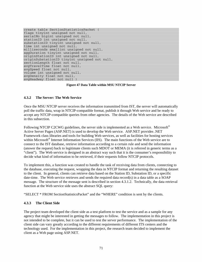
71

create table SectionStatisticsPacket ( flags tinyint unsigned not null, serialNo bigint unsigned not null, stationID int unsigned not null, substationID tinyint unsigned not null, time int unsigned not null, milliseconds smallint unsigned not null, aggDuration tinyint unsigned not null, originStationID int unsigned not null, originSubstationID tinyint unsigned not null, sectionLength float not null, avgTravelTime float not null, avgSpeed float not null, volume int unsigned not null, avgDensity float not null, avgHeadway float not null )

Figure 47 Data Table within MSU NTCIP Server 4.3.2 The Server: The Web Service Once the MSU NTCIP server receives the information transmitted from IST, the server will automatically poll the traffic data, wrap in NTCIP-compatible format, publish it through Web service and be ready to accept any NTCIP-compatible queries from other agencies. The details of the Web service are described in this subsection. Following NTCIP C2CWG guidelines, the server side is implemented as a Web service. Microsoft® Active Server Pages (ASP.NET) is used to develop the Web service. ASP.NET provides .NET Framework class libraries and tools for building Web services, as well as facilities for hosting services within Microsoft® Internet Information Services (IIS). The main functions of the Web service are to connect to the IST database, retrieve information according to a certain rule and send the information (answer the request) back to legitimate clients such MDOT or MEMA (it is referred in generic terms as a “client”). The Web service is designed in an abstract way such that it is the consumer’s responsibility to decide what kind of information to be retrieved, if their requests follow NTCIP protocols. To implement this, a function was created to handle the task of receiving data from clients, connecting to the database, executing the request, wrapping the data in NTCIP format and returning the resulting dataset to the client. In general, clients can retrieve data based on the Station ID, Substation ID, or a specific date-time. The Web service retrieves and sends the required data record(s) in a data table as a SOAP message. The structure of the message sent is described in section 4.3.1.2. Technically, the data retrieval function at the Web service side uses the abstract SQL query: “SELECT * FROM SectionStatisticsPacket” and the “WHERE” condition is sent by the clients. 4.3.3 The Client Side The project team developed the client side as a test platform to test the service and as a sample for any agency that might be interested in getting the messages to follow. The implementation in this project is not intended to be complete, but it can be used to test the server performance. The implementation of the client side can vary greatly according to the different requirements of different ITS centers and the technology used. For the implementation in this project, the research team decided to implement the client as a Web page using ASP.NET.

72

The client side includes a simple graphical user interface (GUI) that simulates a simple ITS center. Figure 48 shows the main interface of the client:

Figure 48 SOAP Client’s GUI

4.3.4 Operation The implementation of the NTCIP interface in this project acts as the communication server between the new prototype sensor provided by IST and the TMC. The Web service will be deployed on a Web server and connected to the main IST database that stores the traffic information captured by the prototype sensors. The client can be any TMC (e.g., MDOT) that initiates requests to the server as SOAP messages. Each message contains certain information that helps the Web service retrieve the required information from the database. In the design, the project team made sure to give the Web service a generic functionality to serve different requests from different clients. The project team left the specification of the data to be retrieved and how the data will be handled, to the client, so that each client can have their own way to process the data they request. Figure 49 shows where the system fits in a typical real-world implementation.

73

Figure 49 NTCIP SOAP Interface in a Real-world Implementation 4.4 TESTING The test plan for this project was divided into three main stages: local test, remote test and integration test. The scope of this project did not allow for a planned integration test, so only the first and the second stages have been conducted. For the tests corresponding to these two stages, the project team created a dummy IST database; real-time access to this database falls into the integrated test in the proposed next phase of research. In the first stage, the project team conducted a white box system testing using the Web service testing unit provided by Microsoft® in Visual Sudio.NET. This testing unit helped the debugging of the services locally without the need of a complex consumer implementation, something that sped up the debugging process. In the second stage, the project team conducted a remote test using the client to test how the service responds to remote requests from remote clients and how different clients handle the data. To do that, the project team first created a dummy copy of the IST database following the database description provided by IST data structure; the database was created using an SQL server. The database was filled with random data that simulated field stations in the real world.

Traffic Center /Client side

Sending traffic data to the central IST DB at the server

Detector at the field - Data generator

NTCIP Client SOAP

NTCIP Server SOAP

MSU Server/Web service host

IST Server Side/ Database storage

74

The Web service was deployed on a server in the MTRC under a public Web address and connected to the database, and finally, the client was deployed on a different machine connected to the Internet. To conduct the test, multiple data requests were sent from the client to the server over the Internet. The tests included requesting data based on Station ID, Substation ID and date-time. The tests showed that the service was able to receive, parse and respond to the different requests successfully. This test helped simulate a real-world situation in which the service would be hosted on a computer connected to an NTCIP network and would receive multiple data requests from multiple clients.

4.5 NTCIP SUMMARY AND CONCLUSIONS The core objective of this task was to develop a NTCIP compatible interface which provides emergency travel time data sharing capabilities between NTCIP-compatible ITS centers and local/state/federal DHS emergency management centers. The proposed NTCIP interface and the coordination between the ITS centers and the proposed systems under this project will not only improve DHS’s internal operations but will also provide DHS with the capability to coordinate emergency operations with other agencies involved in the transportation and emergency support functions. To create the interface, the project team followed the NTCIP C2C WG recommendations by developing an XML-standard application protocol, which includes SOAP and WSDL. The project team implemented the Web service using ASP.NET, which provides .NET Framework class libraries and tools for building Web services as well as facilities for hosting services within IIS. The system implemented included three main sub-systems, the database which is the standard SQL database, the Web service that connects to the database and serves clients requests and the client, which is a website that was developed to test the service. For the current project, the implementation acts as the communication server between the new sensors prototype database provided by IST and the transportation center. In the future, the Web service will be deployed on a Web server and connected to the main IST database, which stores the traffic information captured by the prototype sensors. The client can be any TMC (e.g., MDOT) that initiates requests to the server as SOAP messages. Each message contains certain information that helps the Web service retrieve the required information from the database. In the design, the project team gave the Web service a generic functionality to serve different requests from different clients. The project team left the specification of the data to be retrieved, and how the data would be handled, to the client, so that each client could have their own way to process the data that is requested.

75

5. SUMMARY, CONCLUSIONS AND FUTURE RESEARCH The overarching goal of this project was to contributing to solve an emergency transportation problem that at the present time is prevalent in any event that requires a vehicular evacuation in large geographic areas. There are many instances in which it is possible to plan ahead for an emergency evacuation (e.g., an explosion at a chemical processing facility or a hurricane). For those cases, if an accident (or an attack) were to happen, then the best evacuation plan for the prevailing network and weather conditions would be deployed. In other cases (e.g., the derailment of a train transporting hazardous materials), there may not be any previously developed plan to be implemented, and decisions must be made ad-hoc on how to proceed with an emergency evacuation. In both situations, the availability of real-time traffic information plays a critical role in the management of the evacuation operations. To improve public safety during a vehicular emergency evacuation, it is necessary to detect losses of road capacity (due to incidents, for example) as early as possible. Once travel time is obtained, re-routing strategies must be determined in real-time and deployed in the field to help dissipate the congestion and to increase the efficiency of the evacuation. Due to cost constraints, only large urban areas have traffic sensor deployments that permit access to some sort of real-time traffic information; any evacuation taking place in any other areas of the country would have to proceed without real-time traffic information. The latter was the focus of this project. Phase A of the project consisted of the development and testing of a prototype system composed of sensors that are engineered in such a way that they can be rapidly deployed in the field where and when they are needed. Each one of these sensors is also equipped with its own power supply and a GPS device to auto-determine its spatial location on the transportation network under surveillance. The system is capable of assessing traffic parameters by identifying and re-identifying vehicles in the traffic stream as they pass over the loop detectors. The system of sensors transmits, through wireless communication, real-time traffic information (travel time and other parameters) to a CCC. The first part of the project centered on the development of the prototype system and a methodology to conduct an assessment of its capabilities. Subsequently, a series of tests, both in a controlled environment and in the field, were conducted to study the feasibility of rapidly deploying the system of traffic sensors and to assess its ability to provide real-time traffic information during an emergency evacuation. Specifically, the tests were aimed at evaluating the performance of the system of sensors under various traffic and weather conditions and roadway environments. The controlled tests (i.e., deployment and testing of the prototype system in a parking lot with very limited traffic) were performed first and the results that were obtained served as the basis to identify flaws in the system and to make the necessary corrections to the prototype. The working prototype that resulted from these R&D activities was then subject to a series of real-world environment tests (FOTs) in the second part of the project. Those FOTs, which were aimed at studying the reliability and accuracy of the system in a more prolonged time frame, were conducted at two sites: Knoxville, Tennessee (using traffic that traveled in and out of an office complex during an entire week) and Starkville, Mississippi at the MSU campus (using traffic generated during college and high-school commencements). The latter, although not exactly the same as an emergency evacuation, provided the opportunity to create scenarios that have many characteristics (e.g., congested roads) that are similar to those encountered during a real evacuation, particularly from the standpoint of traffic.

5.1 LABORATORY AND FIELD OPERATIONAL TESTS SUMMARY In order to achieve the main objectives of this project (i.e., the development and fine-tuning of a prototype system of sensors to collect and distribute traffic information in real time), a battery of tests was designed

76

and conducted. Those tests were divided into two parts: 1) “laboratory environment” tests, i.e., tests that were conducted under highly controlled conditions, and 2) FOTs, i.e., tests that were conducted under similar conditions to those that the sensors will encounter when operating under real-world conditions. In both cases, the testing of the prototype system involved three main tasks: the development of a testing methodology, the collection of data during the tests and the analysis of the information gathered. The analysis of the collected data was performed using statistical techniques to compare baseline measurements of the collected traffic parameters against the same traffic parameters reported by the prototype system. For both the laboratory and FOTs, some analysis of the data was performed concurrently with the tests (i.e., the data was analyzed as it was gathered or immediately thereafter) to allow adjustments to be made to both the data collection procedures and the prototype system itself. Any identified deficiencies in the prototype system were corrected expeditiously; subsequent tests were used to determine if the adjustments made to the prototype had been successful.

5.1.1 Laboratory Tests Three laboratory (i.e., controlled) environment series of tests were conducted during this phase of the project. The first two tests focused mainly on the determination of the parameters (i.e., accuracy and reliability) of the prototype system and on “debugging” the prototype data collection sub-system. For the first test, the main goals were to determine the maximum reliability of the system, to investigate the ability of the sensors to differentiate among different vehicles, and to determine the accuracy of the prototype system in estimating travel time between sensors. The results of this first battery of tests showed a system reliability that was above 92%, and accuracy levels that were above 95%. The purpose of the second laboratory tests was to investigate the ability of the sensors to differentiate among different vehicles under travel patterns that presented a level of stochasticity higher than those used in the first laboratory test. The stochasticity of the tests was increased by introducing vehicle following patterns and travel delays that were randomly assigned before the test. An additional objective of this second laboratory test was to assess the sensitivity of the system to the geometry and anchoring of the loop detectors, which was determined by measuring its reliability and accuracy under the testing conditions. The results of the test indicated that the system presented a high reliability (greater than 84%) and accuracy (greater than 96%), even with loop detectors that were not perfectly anchored to the pavement. The main objective of the third laboratory test was to assess the ability of the prototype system to communicate in real-time the data gathered in the field, including travel time between pairs of sensors, as well as speed, volume and vehicle classification at each one of the prototype sensors. The test showed that each component of the system (i.e., sensor) was able to broadcast its position accurately and provide traffic information in real time to a website. In all cases, the null hypothesis (Ho) stating that the means of the travel-time distributions generated with the GT and P data were the same could only be rejected at a very low confidence level, thus concluding that both travel-time means were the same. After the three laboratory tests were completed, the prototype system was deemed ready to enter the next battery of tests in an environment closer to the one in which it will ultimately operate.

5.1.2 Field Operational Tests Five FOTs were conducted during this phase of the project with the goal of assessing the performance of the prototype system in environments closer to those in which it will normally operate. In all five FOTs the system tested consisted of three prototype sensors (with their GPS and communication subsystems)

77

that were deployed at strategic points on roadways within the geographical area where the tests were to take place. In addition, three cameras deployed in the vicinity of the sensors were used to collect GT data, which served as the baseline for the comparison with the travel-time information provided by the prototype system. The first FOT, which lasted five days, was conducted at the NTRC building in Knoxville, Tennessee in April 2008. The test collected traffic information provided by vehicles going in and out of the building parking lots during office hours. The other four FOTs took place at the main campus of MSU in Starkville, Mississippi in May 2008 during college and high-school commencement ceremonies. Those events were selected with the expectation that high volumes of traffic would be generated by people attending these ceremonies; a situation that would mimic those in which the prototype system would normally operate. In all cases, the data collected in real-time by the prototype system was relayed to a website as it was gathered and was later downloaded for comparison against the GT collected information. As was expected for the real-world tests, the reliability of the system was lower than in the controlled-environment tests (laboratory tests) that were conducted in the first part of the project. The statistical analyses showed that the system presented a reliability of more than 88% for the Tennessee FOT and between 42% and 54% for the MSU FOT. The accuracy was very high in all of the FOTs indicating the ability of the system in determining travel time in real-world environments. In all cases, the null hypothesis (Ho), stating that the means of the travel-time distributions generated with the GT and P data were the same, could only be rejected at a very low confidence level, thus indicating that both travel-time means were the same.

5.2 NTCIP DEVELOPMENT SUMMARY The core objective of this task was to develop a NTCIP compatible interface, which provides emergency travel time data sharing capabilities between NTCIP-compatible ITS centers and local/state/federal DHS emergency management centers. The proposed NTCIP interface and the coordination between the ITS centers and the proposed systems under this project will not only improve DHS’s internal operations, but will also provide DHS with the capability to coordinate emergency operations with other agencies involved in the transportation and emergency support functions. To create the interface, the project team followed the NTCIP C2C WG recommendations by developing an XML-standard application protocol, which includes SOAP and WSDL. The project team implemented the Web service using ASP.NET, which provides .NET Framework class libraries and tools for building Web services as well as facilities for hosting services within IIS. The implemented system included three main sub-systems: the database that is the standard SQL database, the Web service that connects to the database and serves clients requests, and the client, which is a website that was developed to test the service. For the current project, the implementation acts as the communication link between the new prototype sensors database provided by IST, and the transportation center. In the future, the Web service will be deployed on a Web server and connected to the main IST database that stores the traffic information captured by the prototype sensors. The client can be any TMC (e.g., MDOT) that initiates requests to the server as SOAP messages. Each message contains certain information that helps the Web service retrieve the required information from the database. In the design, the project team gave the Web service a generic functionality to serve

78

different requests from different clients. The project team left the specification of the data to be retrieved and how the data would be handled to the client so that each client could have their own way to process the data requested data.

5.3 CONCLUSIONS The first phase of this project showed the feasibility of creating an emergency traffic information system which can be deployed anywhere with minimal advance notice, of which the core components are the new sensors that could provide real-time travel-time information for the evacuation routes. Traffic-related information gathering and distribution plays a critical role in the response phase of any such events because it is paramount to determine the status of the transportation system to help with the decision process and field operations (e.g., routing emergency vehicles around congested areas). The system developed in this project can collect and provide traffic information in real time for both the system managers (transportation agencies, emergency management agencies, law enforcement agencies, fire and rescue agencies, emergency medical service providers, 911 dispatchers and towing companies) and the public. This is a very important and necessary system as pointed out by experts such as Ms. K. Vasconez, Team Leader of the FHWA’s Emergency Transportation Operations group (see Appendix A). The extensive tests conducted in this project covered controlled environments and real-world deployments. In all of the cases tested, the prototype system (composed of three sensors) performed very well showing levels of reliability and accuracy that are in line with or above what will be required during a large-scale emergency evacuation. During such events, many more than three sensors will need to be deployed to have an adequate coverage of the area that is being managed; further testing is necessary to determine how the system behaves under these conditions. However, it is expected that similar results as those obtained in this project will be observed because the basic subsystem is defined by at least two sensors that work together to identify/re-identify vehicles, thus making the system scalable. The project also developed a protocol interface to make it possible for these sensors to be integrated into any TMC. The interface was implemented as a Web service that receives different data requests from different clients, connects to the database, retrieves the requested data and finally sends the data back to the TMC clients. Web services are implemented using SOAP protocol, which facilitates the process of data communication over the Internet. The system was successfully tested using a dummy database and a simulated client.

5.4 FUTURE RESEARCH AND DEVELOPMENT

The results of this first phase show that the prototype sensors are reliable and accurate for the type of application that is the focus of this project. During an emergency evacuation, these sensors would be deployed by law enforcement or emergency management personnel who are likely to be performing many other activities. Therefore, in order to make this a viable tool to be used in emergency evacuations, the loop detectors (i.e., the component of the sensors that lays on the pavement and captures the vehicles’ inductive signatures) need to be very easy to deploy—for example by simply rolling the loop detector across the road and connecting it to the control box. One consequence of this is that the loop detectors will lay in different relative positions to the stream of traffic, and, therefore, they may capture inductive signatures that will look different, even if they belong to the same vehicle. This problem needs to be studied in further detail. Another issue to be studied is that of the sensors self-arrangement into a network. In the first phase of the project, the different instrumented roadway segments, characterized by upstream and downstream

79

sensors, were defined manually. In a real-world deployment, this is impractical. However, because the sensors have a GPS device and they broadcast their position, the location information can be integrated with GIS technology to automatically determine the instrumented roadway segments. The problem of where to deploy the sensors to achieve an optimum level of information with the least number of sensors is a dynamic problem and depends on the type of event and the area to be evacuated. This problem also needs to be studied in further detail. The prototype sensors studied in this project will provide just a piece of information, albeit an important one, during an emergency evacuation. For this information to be effective, it needs to be combined and integrated with other technologies. Integration with traffic simulation models will provide the means to determine whether the evacuation is proceeding as predicted and, if traffic management changes are necessary (e.g., due to incidents causing loss of roadway capacity), what are the best re-routing alternatives given the current traffic conditions in the transportation network within the affected area. Other technologies being developed under the SERRI umbrella, such as the evacuation of large sport venues, will also benefit from having real-time traffic information for the area surrounding those stadiums. Integration of the two technologies will provide the means to assess which is the best protective action alternative. For example, in some cases, depending on the type of event being considered and the traffic conditions surrounding a stadium, it may be more appropriate to have an initial shelter in an alternative place deployed, followed by evacuation. The real-time traffic information provided by the sensors developed under this project can help make these decisions. The project team focused on researching and exploring sensor accuracy on laboratory and real-world conditions, although restricted to a few links. In a real evacuation situation, the balance between accuracy and the number of deployed sensors, which determine the cost of data collection, is of fundamental importance. A poorly designed deployment of the sensors may not capture the key parameters needed to optimize the traffic operations during an evacuation, and could impose higher costs than necessary. Therefore, one key objective of future research is the determination of the optimum location of the sensors. The integration of the system with TMCs and CCCs through the NTCIP interface will make it possible for emergency managers and the public to receive travel-time information in real time. Although the NTCIP interface is ready at this point, the entire proposed system needs to be tested with an existing TMC. The project team has already identified the potential locations and TMC systems to conduct future inter-agency tests. The sensor deployability, location, and integration with other systems are issues which could be addressed in a future phase of the project.

80


81

6. ACKNOWLEDGEMENTS We would like to thank the graduate and undergraduate students from the Civil and Environmental Engineering Department of MSU who helped in the data collection phase; Paul Foley, Ebony Lyons, Jennifer Sloan, Jizhan Gou, Di Wu and James Burke and all other individuals who helped accomplish this project. Mike Stoke from MDOT provided us the information about the Mississippi TMC and TMC interfacing capabilities. Mr. Wei Wu from Delcan's Chicago office provided us detailed information about XML/SOAP programming. Ms. Kristine Dechert, a Lecturer in the Department of English, MSU edited the final draft.

82


83

7. BIBLIOGRAPHY Avery, P.R, C. P. Thomas, Y. Wang, and G. S. Rutherford, (2003) “Development of a Length-based Vehicle Classification System Using Uncalibrated Video Cameras,” Presented at Transportation Research Board 2004 Annual Meeting. Paper -002848

Cheu, R. L., Qi, H. and Lee, D-H, (2003) “A Mobile Sensor and Sample-based Algorithm for Freeway Incident Detection,” Transportation Research Record 1811, pp 12-20

Devore, J., “Probability and Statistics for Engineering and the Sciences,” Second Edition, 1987.

Gupte, S., Osama Masoud, Robert F. K. Martin, and Nikolaos P. Papanikolopoulos, (2002) “Detection and Classification of Vehicles,” IEEE Transactions on Intelligent Transportation Systems, Volume3, No. 1.

MacCarley, C.A. et al, (1992) “Evaluation of Video Image Processing Systems for Traffic Detection,” Transportation Research Record 1360, pp 46-49

Malik, J. and Stuart Russell, (1996) Traffic Surveillance and Detection Technology Development: New Traffic Sensor Technology, Final Report UCB-ITS-PRR-97-6, Berkeley, California: California PATH Program.

Mimbela, L. Y. and Lawrence A. Klein, (2000) Summary of Vehicle Detection and Surveillance Technologies Used in Intelligent Transportation Systems, Report, Federal Highway Administration Intelligent Transportation System Joint Program Office, available at http://www.fhwa.dot.gov/ohim/tvtw/vdstits.pdf (last accessed December 15th, 2009).

Michael R. Moore, Stephen F. Smith, and Kang Lee, (2001) "The Next Step — Wireless IEEE 1451 Smart Sensor Networks," Sensors Magazine., v. 18, n.9, pp. 35–43.

Oh, C., Stephen G. Ritchie and Shin-Ting Jeng, (2004) “Vehicle Re-identification Using Heterogeneous Detection Systems,” Presented at 2004 TRB Annual Meeting. Paper2004-002900

Sheskin, D., “Handbook of Parametric and Nonparametric Statistical Procedures,” Third Edition, 2003.

NTCIP 9001, National Transportation Communications for ITS Protocol, The NTCIP Guide v03.02b, October 2002.

NTCIP 2306. Application Profile for XML in ITS Center to Center Communications (AP-C2CXML). NTCIP V1.06. Posted on Janurary 8, 2007. http://www.ntcip.org/library/standards/default.asp?documents=yes&qreport=no&standard=2306 . Accessed on December 15, 2009. NTCIP 9010 v01.07, National Transportation Communications for ITS Protocol. XML in ITS C2C Communications, October 2003.

IST Communication Data Structures for Vehicle Classification and Tracking, Inductive Signature Technologies, 2007.

84


APPENDIX A. PROJECT ENDORSEMENT FROM OUTSIDE ORGANIZATIONS


A-3

APPENDIX A. PROJECT ENDORSEMENT FROM OUTSIDE ORGANIZATIONS

“On behalf of the Federal Highway Administration, we find this proposal to have significant merit. As you know, the last Surface Transportation Legislation (SAFETEA-LU) tasked FHWA with conducting a study of evacuation plans in the Gulf Coast areas as a post-Katrina effort. This activity was to be conducted in concert with the Department of Homeland Security and was conducted concurrent to DHS' National Plan Review effort. In both studies, respondents indicated that a gap exists in the nation's ability to collect real-time highway information to aid in evacuating populations.

There are some efforts to build real time data collection into models, but modeling is not particularly useful during disaster operations and the means to collect real-time data does not exist in many areas of the country. As a result, I find that--based on my knowledge of what is being done in the area of evacuations--your proposal is unique and has the potential to make a significant impact on local jurisdictions' abilities to support evacuations.”

“Moreover, it complements FHWA's current efforts to provide guidance on the benefits and methods of interconnecting Transportation Management Centers, Emergency Operations Centers and Fusion Centers so that critical information can be shared. Real time transportation data that would be provided by the road sensors would greatly enhance the connectivity of these three operations centers.

As a result, FHWA does endorse this proposal.” Kimberly C. Vásconez, M.P.I.A. Team Leader, Emergency Transportation Operations Office of Operations, Federal Highway Administration Department of Transportation 202-366-1559 703- 389-3312/mobile 202-366-3302/FAX 202-366-1560 [email protected] Submitted to ORNL on August 13th, 2008, 16:43.


Documents

RTEE Phase A Final Report - INFO - Home · ORNL/TM-2009/111 Real-Time Traffic Information for Emergency Evacuation Operations: Phase A Final Report December 2009 Prepared by Oscar