Embed Size (px)
Citation preview
Rotated Versions of the Jablonowski Steady-State andBaroclinic Wave Test Cases: A Dynamical CoreIntercomparison
Peter H. Lauritzen1, Christiane Jablonowski2, Mark A. Taylor3 and Ramachandran D. Nair4
1Climate and Global Dynamics, National Center for Atmospheric Research, Boulder, Colorado, USA
2University of Michigan, Department of Atmospheric, Oceanic and Space Sciences, Ann Arbor, Michigan, USA
3Sandia National Laboratories, Albuquerque, New Mexico, USA
4Institute for Mathematics Applied to Geosciences, National Center for Atmospheric Research, Boulder, Colorado, USA
Manuscript submitted 5 August 2009; in final form 27 November 2009
The Jablonowski test case is widely used for debugging and evaluating the numerical characteristics of global
dynamical cores that describe the fluid dynamics component of Atmospheric General Circulation Models.
The test is defined in terms of a steady-state solution to the equations of motion and an overlaid
perturbation that triggers a baroclinically unstable wave. The steady-state initial conditions are zonally
symmetric. Therefore, the test case design has the potential to favor models that are built upon regular
latitude-longitude or Gaussian grids. Here we suggest rotating the computational grid so that the balanced
flow is no longer aligned with the computational grid latitudes. Ideally the simulations should be invariant
under rotation of the computational grid. Note that the test case only requires an adjustment of the Coriolis
parameter in the model code.
The rotated test case has been exercised by six dynamical cores. In addition, two of the models have been
tested with different vertical coordinates resulting in a total of eight model variants. The models are built
with different computational grids (regular latitude-longitude, cubed-sphere, icosahedral hexagonal/
triangular) and use very different numerical schemes. The test-case is a useful tool for debugging, assessing
the degree of anisotropy in the numerical methods and grids, and evaluating the numerical treatment of the
pole points since the rotated test case directs the flow directly over the geographical poles. Special treatments
such as polar filters are therefore more exposed in this rotated test case.
DOI:10.3894/JAMES.2010.2.15
1. Introduction
The need for developing global test cases for dynamical
cores is becoming increasingly important as modeling
groups move towards seamless modeling systems where
the same flow solvers are intended for both high weather
resolutions as well as for coarser climate resolutions. Hence
the dynamical core should be accurate across an even wider
range of scales. To meet the requirements of a high degree of
computational parallelism and scalability in the numerical
algorithms non-traditional spherical grids, that are more
isotropic than the widely used regular latitude-longitude
grids, are being explored. In addition, novel numerical
techniques are being assessed by the global atmospheric
modeling community. All these factors raise questions about
the accuracy of these new models as compared to traditional
approaches that have been tested and used extensively
during the last 20–30 years.
At any resolution it is inevitable that a numerical method
introduces errors and thereby misrepresent the flow in some
way. It is hard to distinguish cause and effect in model runs
with parameterized physical processes. Therefore, running
idealized test cases have become standard during model
development. Standard test cases for passive tracer transport
(see Machenhauer et al. 2008 for an overview) and two-
dimensional shallow water tests (e.g., Williamson et al. 1992,
Galewsky et al. 2004, Lauter et al. 2005) are well established
in the atmospheric modeling community whereas global test
cases for three dimensional models are not as widespread. A
global test case gaining popularity was recently proposed by
Jablonowski (2004) and examined by Jablonowski and
This work is licensed under a Creative
Commons Attribution 3.0 License.
To whom correspondence should be addressed.
Peter Hjort Lauritzen, Climate and Global Dynamics, National Center for
Atmospheric Research, 1850 Table Mesa Drive, Boulder, CO, 80305, USA
J. Adv. Model. Earth Syst., Vol. 2, Art. #15, 34 pp.
JOURNAL OF ADVANCES IN MODELING EARTH SYSTEMS
Williamson (2006a; hereafter referred to as JW06). It consists
of a steady-state solution and a baroclinic wave resulting from
adding a perturbation to the steady-state initial condition. The
Jablonowski test case targets the large scale (hydrostatic)
performance of the model and its ability to retain a balanced
flow. An analytic solution exists for the steady-state test case
provided the model utilizes a hydrostatic or non-hydrostatic
shallow-atmosphere equation set. No analytic solution exists
for the baroclinic wave test and therefore the ‘exact’ solution
must be approximated numerically. The test is deterministic
and convergence can be established based on an ensemble of
high resolution reference solutions (JW06). Other idealized
test cases for three-dimensional dynamical cores have also
recently been proposed by Polvani et al. (2004), Staniforth and
White (2008b), Staniforth and White (2008c) and
Jablonowski et al. (2011). In addition, test cases targeting
the smaller scale and non-hydrostatic performance of the
dynamical cores were suggested by Wedi and Smolarkiewicz
(2009). Global non-hydrostatic models should also be able to
retain large scale balances in the flow. It is therefore expected
that the non-hydrostatic models run at hydrostatic resolutions
(scales) converge to the hydrostatic model reference solutions.
Here we propose a variant of the Jablonowski test cases
where the physical flow remains the same but the computa-
tional grid is rotated with respect to the physical flow.
Ideally the dynamical core should be invariant under rota-
tion of the computational grid. However, usually the
numerical algorithms are less challenged when the flow is
aligned or quasi-aligned with the computational grid in
contrast to flows that predominantly traverse the computa-
tional grid lines at a slantwise angle. Therefore the
Jablonowski test cases somewhat favors regular latitude-
longitude grids since the flow is predominantly parallel to
the latitude circles throughout the domain. The grid rota-
tions suggested in this paper are schematically explained in
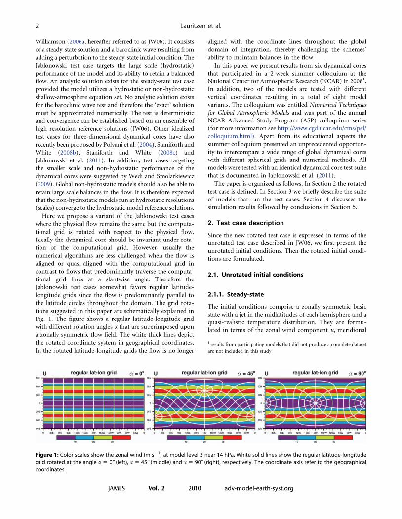
Fig. 1. The figure shows a regular latitude-longitude grid
with different rotation angles a that are superimposed upon
a zonally symmetric flow field. The white thick lines depict
the rotated coordinate system in geographical coordinates.
In the rotated latitude-longitude grids the flow is no longer
aligned with the coordinate lines throughout the global
domain of integration, thereby challenging the schemes’
ability to maintain balances in the flow.
In this paper we present results from six dynamical cores
that participated in a 2-week summer colloquium at the
National Center for Atmospheric Research (NCAR) in 20081.
In addition, two of the models are tested with different
vertical coordinates resulting in a total of eight model
variants. The colloquium was entitled Numerical Techniques
for Global Atmospheric Models and was part of the annual
NCAR Advanced Study Program (ASP) colloquium series
(for more information see http://www.cgd.ucar.edu/cms/pel/
colloquium.html). Apart from its educational aspects the
summer colloquium presented an unprecedented opportun-
ity to intercompare a wide range of global dynamical cores
with different spherical grids and numerical methods. All
models were tested with an identical dynamical core test suite
that is documented in Jablonowski et al. (2011).
The paper is organized as follows. In Section 2 the rotated
test case is defined. In Section 3 we briefly describe the suite
of models that ran the test cases. Section 4 discusses the
simulation results followed by conclusions in Section 5.
2. Test case description
Since the new rotated test case is expressed in terms of the
unrotated test case described in JW06, we first present the
unrotated initial conditions. Then the rotated initial condi-
tions are formulated.
2.1. Unrotated initial conditions
2.1.1. Steady-state
The initial conditions comprise a zonally symmetric basic
state with a jet in the midlatitudes of each hemisphere and a
quasi-realistic temperature distribution. They are formu-
lated in terms of the zonal wind component u, meridional
Figure 1: Color scales show the zonal wind (m s21) at model level 3 near 14 hPa. White solid lines show the regular latitude-longitudegrid rotated at the angle a 5 0˚(left), a 5 45˚(middle) and a 5 90˚(right), respectively. The coordinate axis refer to the geographicalcoordinates.
1 results from participating models that did not produce a complete dataset
are not included in this study
2 Lauritzen et al.
JAMES Vol. 2 2010 adv-model-earth-syst.org
wind component v, temperature T, surface pressure ps and
surface geopotential Ws. Extensions to other prognostic
variable sets are straightforward. In addition, we assume
vertical coordinates that are typically used in General
Circulation Models (GCMs) today. These are the pressure-
based s 5 p/ps (Phillips 1957) coordinate or an g (hybrid s– p; Simmons and Burridge 1981) vertical coordinate as
defined by
p l, Q, gð Þ~A gð Þp0zB gð Þps l, Qð Þ: ð2:1Þ
The interface coefficients A and B (half indices) are given in
Table 1, l [0, 2p] and Q [2p/2, p/2] denote the
longitudinal and latitudinal directions, the reference pres-
sure p0 is set to 1000 hPa, and the initial surface pressure ps
is constant and set to ps 5 1000 hPa. Throughout this
paper, 26 vertical model levels are used. The hybrid coord-
inate g [0, 1] is unity at the surface and approaches a
constant at the model top. Note that the value of p0 might
not be standard in all GCMs that utilize the hybrid vertical
coordinate system.
The flow field is comprised of two symmetric non-
divergent zonal jets in the midlatitudes:
usteady l, Q, gð Þ~u0 cos32gv sin2 2Qð Þ, ð2:2Þ
vsteady l, Q, gð Þ~0, ð2:3Þ
where gv is defined as gv 5 0.5(g 2 g0)p, g0 5 0.252 is the
center position of the jet, and the maximum amplitude u0 is
set to 35 m s21. This velocity distribution resembles the
zonal-mean time-mean jet streams in the troposphere. For
non-hydrostatic models the vertical velocity is set to zero.
The temperature distribution consists of a horizontal-
mean temperature and a horizontal variation at each level.
The horizontally averaged temperature �TT gð Þ is given by
�TT gð Þ~ T0 gRdC
g for gs§g§gt
T0 gRdC
g zDT gt{gð Þ5 for gtwg
8<: ð2:4Þ
with the surface level gs 5 1, tropopause level gt 5 0.2 and
horizontal-mean temperature at the surface T0 5 288 K. The
temperature lapse rate C is set to 0.005 K m21 which is
similar to the observed diabatic lapse rate. The empirical
temperature difference DT is set to 4.8 6 105 K, Rd 5
287.04 J (kg K)21 represents the ideal gas constant for dry
air and g 5 9.80616 m s22 is the gravitational acceleration.
The three-dimensional temperature distribution is then
defined by
T l, Q, gð Þ~�TT gð Þz 3
4
g p u0
Rd
sin gv cos12 gv|
{2sin6 Q (cos2 Qz1
3)z
10
63
� �|
�
2 u0 cos32 gvz
8
5cos3 Q (sin2 Qz
2
3){
p
4
� �a V
�,
ð2:5Þ
where V 5 7.29212 6 1025 s21 is the Earth’s angular
velocity and a 5 6.371229 6 106 m is the radius of the
Earth. The geopotential W 5 gz completes the description of
the steady-state initial conditions where z symbolizes the
elevation of a model level g. The total geopotential distri-
bution comprises the horizontal-mean geopotential �WW and a
horizontal variation at each level. This is analogous to the
description of the temperature field. The geopotential is
given by
W l, Q, gð Þ~�WW gð Þzu0 cos32 gv|
{2sin6 Q (cos2 Qz1
3)z
10
63
� �|
�
u0 cos32 gvz
8
5cos3 Q (sin2 Qz
2
3){
p
4
� �a V
�,
ð2:6Þ
with
�WW gð Þ~To g
C 1{gRdC
g
� �for gs§g§gt
To g
C 1{gRdC
g
� �{K for gtwg
8><>: ð2:7Þ
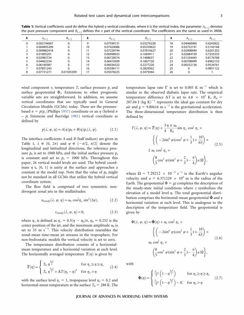
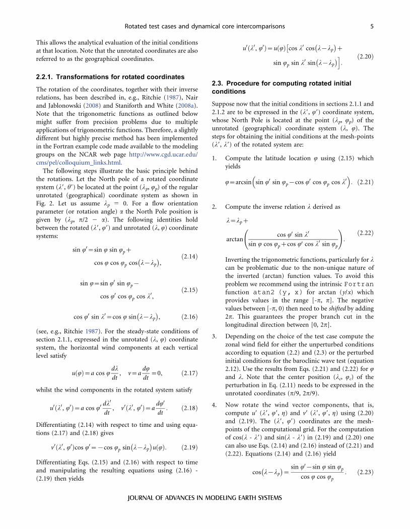
Table 1: Vertical coefficients used do define the hybrid g-vertical coordinate, where k is the vertical index, the parameter Akz12
denotesthe pure pressure component and Bkz1
2defines the s part of the vertical coordinate. The coefficients are the same as used in JW06.
k Akz12
Bkz12
k Akz12
Bkz12
k Akz12
Bkz12
0 0.002194067 0. 9 0.07590131 0.03276228 18 0.04468960 0.42438221 0.004895209 0. 10 0.07424086 0.05359622 19 0.03752191 0.51431682 0.009882418 0. 11 0.07228744 0.07810627 20 0.02908949 0.62012023 0.01805201 0. 12 0.06998933 0.1069411 21 0.02084739 0.72353554 0.02983724 0. 13 0.06728574 0.1408637 22 0.01334443 0.81767685 0.04462334 0. 14 0.06410509 0.1807720 23 0.00708499 0.89621536 0.06160587 0. 15 0.06036322 0.2277220 24 0.00252136 0.95347617 0.07851243 0. 16 0.05596111 0.2829562 25 0. 0.98511228 0.07731271 0.01505309 17 0.05078225 0.3479364 26 0. 1.
Rotated test cases and dynamical core intercomparisons 3
JOURNAL OF ADVANCES IN MODELING EARTH SYSTEMS
where
K~Rd DT| ln(g
gt
)z137
60
� �g5
t
�
{5g4t gz5g3
t g2{10
3g2
t g3z5
4gt g
4{1
5g5
�:
ð2:8Þ
This formulation enforces the hydrostatic balance ana-
lytically and ensures the continuity of the geopotential at
the tropopause level gt. In hydrostatic models with pres-
sure-based vertical coordinates, it is only necessary to
initialize the surface geopotential Ws 5 gzs. It balances
the non-zero zonal wind at the surface with surface
elevation zs and is determined by setting g 5 gs in (2.6).
This leads to the following equation for the surface geo-
potential
Ws l, Qð Þ~u0 cos32 gs{g0ð Þ p
2
� �|
{2sin6 Q (cos2 Qz1
3)z
10
63
� �|
�
u0 cos32 gs{g0ð Þ p
2
� �z
8
5cos3 Q (sin2 Qz
2
3){
p
4
� �a V
�:
ð2:9Þ
Note that Ws is a function of latitude only. The geopotential
equation (2.6) can fully be utilized for dynamical cores with
height-based vertical coordinates. Then, a root-finding
algorithm is recommended to determine the corresponding
g-level for any given height z. This iterative method, which
is also applicable to isentropic vertical coordinates, is out-
lined in the Appendix of JW06. The resulting g-level is
accurate to machine precision and can consequently be used
to compute the initial data set.
The test design guarantees static, inertial and symmetric
stability properties, but is unstable with respect to baroclinic
or barotropic instability mechanisms.
2.1.2. Baroclinic wave
A baroclinic wave can be triggered if the initial conditions
for the steady-state test described in the previous subsection
are overlaid with a perturbation. Here a perturbation with a
Gaussian profile is selected and centered at (lc, Qc) 5 (p/9,
2p/9) which points to the location (20 E,40 N). The per-
turbation overlays the zonal wind field. The zonal wind
perturbation upert is given by
upert l, Q, gð Þ~up exp {r
R
� �2
� �ð2:10Þ
with the great circle distance r
r~a arccos sin Qc sin Qzcos Qc cos Q cos l{lcð Þð Þ: ð2:11Þ
The radius of the perturbation is R 5 a/10. The maximum
perturbation amplitude is set to up 5 1 m s21. It is super-
imposed on the balanced zonal wind field (2.2) by
adding upert to the wind field at each grid point at all model
levels:
uwave l, Q, gð Þ~usteadyzupert : ð2:12Þ
The meridional wind component is zero as in the steady-
state initial condition: vwave 5 vsteady 5 0.
The baroclinic wave, although idealized, represents very
realistic flow features. Strong temperature fronts develop
that are associated with the evolving low and high pressure
systems. Note that the baroclinic wave test case does not
have an analytic solution. Therefore, high resolution ref-
erence solutions and their uncertainties are used (JW06).
2.2. Rotated initial conditions
The rotated initial conditions are formulated in terms of the
unrotated initial conditions. The physical flow remains the
same but the computational grid is rotated with respect to
the physical flow. However, two changes are necessary. First,
because of the rotations the Coriolis parameter f is a
function of both latitude Q and longitude h:
f l, Qð Þ~2V {cos l cos Q sin azsin Q cos að Þ: ð2:13Þ
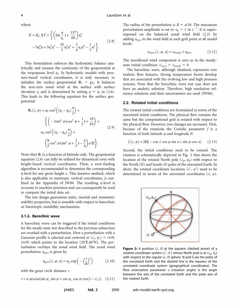
Second, the initial conditions need to be rotated. The
rotation is schematically depicted in Fig. 2 that shows the
location of the rotated North pole (lp, Qp) with respect to
the North (N) and South (S) poles of the unrotated Earth. In
short, the rotated coordinate locations (l9, Q9) need to be
determined in terms of the unrotated coordinates (l, Q).
Figure 2: A position (l, h) at the equator (dashed arrow) of arotated coordinate system (l9, h9) whose North pole is at (lp, hp)with respect to the regular (l, h) sphere. N and S are the poles ofthe unrotated Earth and the dashed line is the equator of theunrotated coordinate system (geographical coordinates). Theflow orientation parameter a (rotation angle) is the anglebetween the axis of the unrotated Earth and the polar axis ofthe rotated Earth.
4 Lauritzen et al.
JAMES Vol. 2 2010 adv-model-earth-syst.org
This allows the analytical evaluation of the initial conditions
at that location. Note that the unrotated coordinates are also
referred to as the geographical coordinates.
2.2.1. Transformations for rotated coordinates
The rotation of the coordinates, together with their inverse
relations, has been described in, e.g., Ritchie (1987), Nair
and Jablonowski (2008) and Staniforth and White (2008a).
Note that the trigonometric functions as outlined below
might suffer from precision problems due to multiple
applications of trigonometric functions. Therefore, a slightly
different but highly precise method has been implemented
in the Fortran example code made available to the modeling
groups on the NCAR web page http://www.cgd.ucar.edu/
cms/pel/colloquium_links.html.
The following steps illustrate the basic principle behind
the rotations. Let the North pole of a rotated coordinate
system (l9, h9) be located at the point (lp, Qp) of the regular
unrotated (geographical) coordinate system as shown in
Fig. 2. Let us assume lp 5 0. For a flow orientation
parameter (or rotation angle) a the North Pole position is
given by (lp, p/2 2 a). The following identities hold
between the rotated (l9, Q9) and unrotated (l, Q) coordinate
systems:
sin Q0~sin Q sin Qpz
cos Q cos Qp cos l{lp
� ,
ð2:14Þ
sin Q~sin Q0 sin Qp{
cos Q0 cos Qp cos l0,ð2:15Þ
cos Q0 sin l0~cos Q sin l{lp
� , ð2:16Þ
(see, e.g., Ritchie 1987). For the steady-state conditions of
section 2.1.1, expressed in the unrotated (l, Q) coordinate
system, the horizontal wind components at each vertical
level satisfy
u Qð Þ~a cos Qdl
dt, v~a
dQ
dt~0, ð2:17Þ
whilst the wind components in the rotated system satisfy
u0 l0, Q0ð Þ~a cos Q0dl0
dt, v0 l0, Q0ð Þ~a
dQ0
dt: ð2:18Þ
Differentiating (2.14) with respect to time and using equa-
tions (2.17) and (2.18) gives
v0 l0, Q0ð Þcos Q0~{cos Qp sin l{lp
� u Qð Þ: ð2:19Þ
Differentiating Eqs. (2.15) and (2.16) with respect to time
and manipulating the resulting equations using (2.16) -
(2.19) then yields
u0 l0, Q0ð Þ~u Qð Þ cos l0 cos l{lp
� z
sin Qp sin l0 sin l{lp
� i:
ð2:20Þ
2.3. Procedure for computing rotated initialconditions
Suppose now that the initial conditions in sections 2.1.1 and
2.1.2 are to be expressed in the (l9, Q9) coordinate system,
whose North Pole is located at the point (lp, Qp) of the
unrotated (geographical) coordinate system (l, Q). The
steps for obtaining the initial conditions at the mesh-points
(l9, l9) of the rotated system are:
1. Compute the latitude location Q using (2.15) which
yields
Q~arcsin sin Q0 sin Qp{cos Q0 cos Qp cos l0� �
: ð2:21Þ
2. Compute the inverse relation l derived as
l~lpz
arctancos Q0 sin l0
sin Q cos Qpzcos Q0 cos l0 sin Qp
!:
ð2:22Þ
Inverting the trigonometric functions, particularly for lcan be problematic due to the non-unique nature of
the inverted (arctan) function values. To avoid this
problem we recommend using the intrinsic Fortranfunction atan2 (y, x) for arctan (y/x) which
provides values in the range [-p, p]. The negative
values between [-p, 0) then need to be shifted by adding
2p. This guarantees the proper branch cut in the
longitudinal direction between [0, 2p].
3. Depending on the choice of the test case compute the
zonal wind field for either the unperturbed conditions
according to equation (2.2) and (2.3) or the perturbed
initial conditions for the baroclinic wave test (equation
2.12). Use the results from Eqs. (2.21) and (2.22) for Qand l. Note that the center position (lc, Qc) of the
perturbation in Eq. (2.11) needs to be expressed in the
unrotated coordinates (p/9, 2p/9).
4. Now rotate the wind vector components, that is,
compute u9 (l9, Q9, g) and v9 (l9, Q9, g) using (2.20)
and (2.19). The (l9, Q9) coordinates are the mesh-
points of the computational grid. For the computation
of cos(l - l9) and sin(l - l9) in (2.19) and (2.20) one
can also use Eqs. (2.14) and (2.16) instead of (2.21) and
(2.22). Equations (2.14) and (2.16) yield
cos l{lp
� ~
sin Q0{sin Q sin Qp
cos Q cos Qp
: ð2:23Þ
Rotated test cases and dynamical core intercomparisons 5
JOURNAL OF ADVANCES IN MODELING EARTH SYSTEMS
sin l{lp
� ~
cos Q0 sin l0
cos Q: ð2:24Þ
5. Compute the scalar fields T9 (l9, Q9, g) and (Ws)9 (l9,
Q9, g) in the rotated system by using the result of (2.21)
in the temperature equation (2.5) and the expression
for the surface geopotential (2.9).
This completes the definition of the rotated initial con-
ditions for the steady-state and baroclinic wave test cases.
2.4. Test case strategy
We suggest the following test strategy for the steady-state
test case. The dynamical core is initialized with the balanced
initial conditions and run for 30 model days at varying
horizontal resolutions and rotation angles a 5 0 , 45 , 90 .
Here we assess the convergence with resolution and the
dependence of the simulated solution on the rotation angle.
Ideally the model results should be invariant under rotation.
Any shortcomings with regard to rotation of the computa-
tional grid are due to lack of isotropy in the model. Note
that a discretization scheme on an anisotropic grid can be
isotropic (as is the case for the spectral transform method)
and that a quasi-isotropic grid (such as the icosahedral type
grids described below) not necessarily guarantees that the
model dynamics is isotropic.
In addition, different horizontal resolutions should be
assessed for the baroclinic wave test case to estimate the
convergence characteristics. The results should also be
examined as a function of rotation angle a 5 0 , 45 , 90 .
The baroclinic wave starts growing observably around day 4
and evolves rapidly thereafter with explosive cyclogenesis at
model day 8. The wave train breaks after day 9 and generates
a full circulation in both hemispheres between day 20–30
depending on the model. Therefore the models herein are
run for 15 days to capture the initial and rapid development
stages of the baroclinic disturbance. As observed in JW06
the spread of the numerical solutions increases noticeably
from model day 12 onwards indicating a predictability limit
of the test case.
Here all models are run at two resolutions. The low
resolution simulations utilize a grid spacing of approxi-
mately 2˚ at the model equator, the high resolution corre-
sponds to a grid spacing of about 1˚ at the model equator.
For the baroclinic wave test case we use 7 high-resolution
reference solutions. High resolution reference solutions
with different models still produce a certain spread in the
solution. Therefore, we use the uncertainty of the reference
solution as defined in JW06 to define convergence (see
Section 4.2 for more details). When the ,2 errors are below
the uncertainty of the reference solutions given in JW06 the
model is within the spread of the reference solutions and
we can no longer term one model more accurate than
another.
3. Models
Below is a brief description of the dynamical cores assessed
in this paper. The corresponding model abbreviations used
in this paper are listed in Table 2. The metadata for the
models are given in Tables 3, 4 and 5. The definitions of the
metadata entries are defined in the Appendix. The model
metadata has been developed in collaboration with the Earth
System Curator and Earth System Grid teams at NCAR.
Models defined on three different spherical grids are con-
sidered: Regular or Gaussian latitude-longitude (Fig. 3a),
cubed-sphere (Fig. 3b) and icosahedral grids (Fig. 3c). For
the icosahedral class of grids one can either discretize on
hexagons-pentagons or triangles. Both types of icosahedral
grids are used by models in this ensemble.
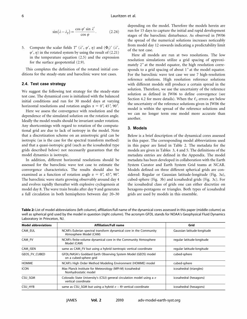
Table 2: List of model abbreviations (left column), affiliation/full name of the dynamical cores assessed in this paper (middle column) aswell as spherical grid used by the model in question (right column). The acronym GFDL stands for NOAA’s Geophysical Fluid DynamicsLaboratory in Princeton, NJ.
Model abbreviations Affiliation/Full name Grid
CAM_EUL NCAR’s Eulerian spectral transform dynamical core in the CommunityAtmosphere Model (CAM)
Gaussian latitude-longitude
CAM_FV NCAR’s finite-volume dynamical core in the Community AtmosphereModel (CAM)
regular latitude-longitude
CAM_ISEN same as CAM_FV but using a hybrid isentropic vertical coordinate regular latitude-longitude
GEOS_FV_CUBED GFDL/NASA’s Goddard Earth Observing System Model (GEOS) modelon a cubed-sphere grid
cubed-sphere
HOMME NCAR’s High Order Method Modeling Environment (HOMME) model cubed-sphere
ICON Max Planck Institute for Meteorology (MPI-M) IcosahedralNonhydrostatic model
icosahedral (triangles)
CSU_SGM Colorado State University’s (CSU) general circulation model using a svertical coordinate
icosahedral (hexagons)
CSU_HYB same as CSU_SGM but using a hybrid s – H vertical coordinate icosahedral (hexagons)
6 Lauritzen et al.
JAMES Vol. 2 2010 adv-model-earth-syst.org
3.1. Latitude-longitude grid models
The two dynamical cores defined on a regular or Gaussian
latitude-longitude grid are part of NCAR’s Community
Atmosphere Model (CAM) version 3 (Collins et al. 2006).
CAM_EUL is based on a spectral transform method on a
Gaussian grid whereas the two model variants CAM_FV and
CAM_ISEN are based on the Lin (2004) finite-volume
approach with a floating Lagrangian coordinate in the
vertical and regular latitude-longitude grid in the horizontal
direction. The latter two utilize the hybrid sigma-pressure
coordinates (CAM_FV) or isentropic coordinates (Chen
and Rasch 2010) as their reference grids. The prognostic
variables are interpolated back to the reference grid peri-
odically (every 4–10 time steps).
The Eulerian spectral transform dynamical core
CAM_EUL is based on the traditional vorticity-divergence
form using the three-time-level semi-implicit Leapfrog
time-stepping method. To damp the computational mode
of the Leap-frog time-stepping scheme a Robert-Asselin
filter (Asselin 1972) is applied which formally reduces the
time-stepping scheme to first order. The horizontal approxi-
mation is based on spectral transforms and a quadratically
unaliased transform grid with triangular truncation. In the
vertical direction, centered finite differences are utilized.
Note that the spherical harmonic functions are invariant
under rotation. The horizontal resolution is referred to as
T42, T85, etc. that denotes the triangular truncation with
the total wave numbers 42 and 85, respectively. The corres-
ponding Gaussian grids have 64 6 128 and 128 6 256
(latitude 6 longitude) grid points, resulting in a grid
spacing of < 2.8˚ (T42) and < 1.4˚ (T85), respectively. As
argued in Williamson (2008) these spectral resolutions are
comparable to other grid-point based dynamical cores with
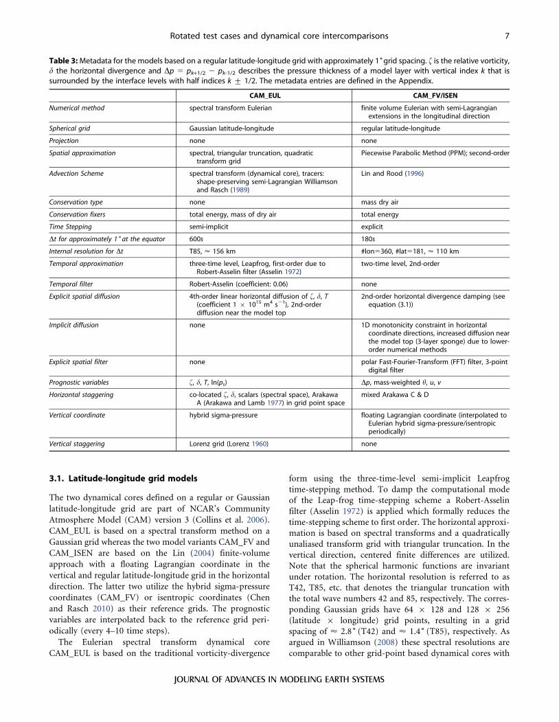
Table 3: Metadata for the models based on a regular latitude-longitude grid with approximately 1˚grid spacing. f is the relative vorticity,d the horizontal divergence and Dp 5 pk+1/2 2 pk-1/2 describes the pressure thickness of a model layer with vertical index k that issurrounded by the interface levels with half indices k ¡ 1/2. The metadata entries are defined in the Appendix.
CAM_EUL CAM_FV/ISEN
Numerical method spectral transform Eulerian finite volume Eulerian with semi-Lagrangianextensions in the longitudinal direction
Spherical grid Gaussian latitude-longitude regular latitude-longitude
Projection none none
Spatial approximation spectral, triangular truncation, quadratictransform grid
Piecewise Parabolic Method (PPM); second-order
Advection Scheme spectral transform (dynamical core), tracers:shape-preserving semi-Lagrangian Williamsonand Rasch (1989)
Lin and Rood (1996)
Conservation type none mass dry air
Conservation fixers total energy, mass of dry air total energy
Time Stepping semi-implicit explicit
Dt for approximately 1˚ at the equator 600s 180s
Internal resolution for Dt T85, < 156 km #lon5360, #lat5181, < 110 km
Temporal approximation three-time level, Leapfrog, first-order due toRobert-Asselin filter (Asselin 1972)
two-time level, 2nd-order
Temporal filter Robert-Asselin (coefficient: 0.06) none
Explicit spatial diffusion 4th-order linear horizontal diffusion of f, d, T(coefficient 1 6 1015 m4 s21), 2nd-orderdiffusion near the model top
2nd-order horizontal divergence damping (seeequation (3.1))
Implicit diffusion none 1D monotonicity constraint in horizontalcoordinate directions, increased diffusion nearthe model top (3-layer sponge) due to lower-order numerical methods
Explicit spatial filter none polar Fast-Fourier-Transform (FFT) filter, 3-pointdigital filter
Prognostic variables f, d, T, ln(ps) Dp, mass-weighted h, u, v
Horizontal staggering co-located f, d, scalars (spectral space), ArakawaA (Arakawa and Lamb 1977) in grid point space
mixed Arakawa C & D
Vertical coordinate hybrid sigma-pressure floating Lagrangian coordinate (interpolated toEulerian hybrid sigma-pressure/isentropicperiodically)
Vertical staggering Lorenz grid (Lorenz 1960) none
Rotated test cases and dynamical core intercomparisons 7
JOURNAL OF ADVANCES IN MODELING EARTH SYSTEMS
mesh spacings of about 2˚ and 1 . To control the inertial
range of the total kinetic energy spectrum fourth-order
linear horizontal diffusion (also referred to as hyperdiffu-
sion) is applied to the vorticity (f), divergence (d) and
temperature (T). The horizontal and vertical grid staggering
utilizes the Arakawa A (Arakawa and Lamb 1977) and
Lorenz (Lorenz 1960) grid, respectively. The vertical coord-
inate is the traditional hybrid sigma-pressure coordinate. A-
posteriori total mass and total energy fixers are applied to
restore the conservation of these quantities at every time
step. Details about the energy fixer can be found in
Williamson et al. (2009).
CAM_FV is based on a flux-form finite-volume method
that is built upon the Lin and Rood (1996) advection
scheme and a CD-grid approach for the two-dimensional
shallow water equations. The algorithm involves a half-
time-step update on the Arakawa C grid that provides the
time-centered winds to complete a full time step on the
Arakawa D grid (Lin and Rood 1997). The momentum
equations are expressed in their vector-invariant form. The
Eulerian model design has semi-Lagrangian extensions in
the longitudinal direction as documented in Lin and Rood
(1996). The Lin-Rood advection scheme utilizes the mono-
tonic Piecewise Parabolic Method (PPM, Colella and
Woodward 1984) that implicitly prevents grid-scale noise
in the vorticity field through the use of limiters. However,
divergent modes must be controlled through the explicit
application of horizontal divergence damping where the
damping coefficient in CAM_FV is:
n~C L2
Dt, ð3:1Þ
where C 5 1/128 and L2 5 a2DlDh. This avoids a spurious
accumulation of energy at and near the grid scale. In
CAM_FV second-order divergence damping is used with
increasing strength near the model top. To stabilize the
model a one-dimensional digital filter is applied along
longitudes in the midlatitudes (approximately between 36˚N/S to 66˚N/S) and a Fast Fourier Transform (FFT) filter is
used in the polar regions poleward of 69 . The shallow water
system is extended to a three-dimensional hydrostatic model
using a floating Lagrangian vertical coordinate (Lin 2004).
The levels float for a few (4–10) consecutive time steps
before a vertical remapping step maps the variables back to
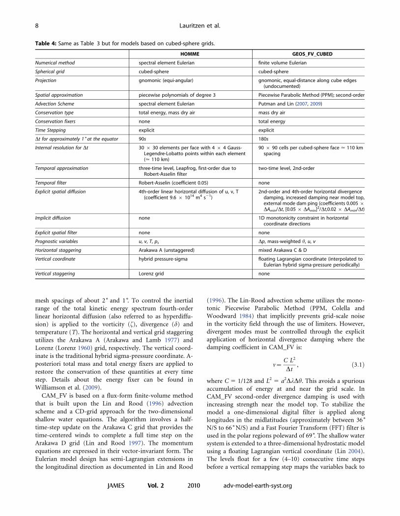
Table 4: Same as Table 3 but for models based on cubed-sphere grids.
HOMME GEOS_FV_CUBED
Numerical method spectral element Eulerian finite volume Eulerian
Spherical grid cubed-sphere cubed-sphere
Projection gnomonic (equi-angular) gnomonic, equal-distance along cube edges(undocumented)
Spatial approximation piecewise polynomials of degree 3 Piecewise Parabolic Method (PPM); second-order
Advection Scheme spectral element Eulerian Putman and Lin (2007, 2009)
Conservation type total energy, mass dry air mass dry air
Conservation fixers none total energy
Time Stepping explicit explicit
Dt for approximately 1˚ at the equator 90s 180s
Internal resolution for Dt 30 6 30 elements per face with 4 6 4 Gauss-Legendre-Lobatto points within each element(< 110 km)
90 6 90 cells per cubed-sphere face < 110 kmspacing
Temporal approximation three-time level, Leapfrog, first-order due toRobert-Asselin filter
two-time level, 2nd-order
Temporal filter Robert-Asselin (coefficient 0.05) none
Explicit spatial diffusion 4th-order linear horizontal diffusion of u, v, T(coefficient 9.6 6 1014 m4 s21)
2nd-order and 4th-order horizontal divergencedamping, increased damping near model top,external mode dam ping (coefficients 0.005 6DAmin/Dt, [0.05 6 DAmin]2/Dt,0.02 6 DAmin/Dt)
Implicit diffusion none 1D monotonicity constraint in horizontalcoordinate directions
Explicit spatial filter none none
Prognostic variables u, v, T, ps Dp, mass-weighted h, u, v
Horizontal staggering Arakawa A (unstaggered) mixed Arakawa C & D
Vertical coordinate hybrid pressure-sigma floating Lagrangian coordinate (interpolated toEulerian hybrid sigma-pressure periodically)
Vertical staggering Lorenz grid none
8 Lauritzen et al.
JAMES Vol. 2 2010 adv-model-earth-syst.org
the reference vertical levels. CAM_FV uses hybrid-sigma
vertical coordinates as the reference grid. The Lin and Rood
(1996) advection scheme is formulated in terms of inner and
outer operators that are applied in the coordinate directions
in a combination to reduce the operator-splitting error. In
CAM_FV the outer operators are based on PPM, and the
inner operators are first-order (upwind scheme). The
stability properties of this scheme are discussed in
Lauritzen (2007). More details on e.g. the time step length
for a 1˚grid spacing are listed in Table 3. Note that the PPM
algorithm is formally third-order accurate in one dimen-
sion, but it reduces to a second-order advection algorithm in
the chosen two-dimensional finite-volume implementation
(i.e., the Lin and Rood, 1996, algorithm). An example of a
two-dimensional extension based on the PPM algorithm
that is third-order is given in, e.g., Ullrich et al. (2010).
CAM_ISEN is an isentropic version of CAM_FV. Instead
of the hybrid sigma-pressure vertical coordinate a hybrid
Table 5: Same as Table 3 but for models based on icosahedral grids. fa is the absolute vorticity, f is the Coriolis parameter.
ICON CSU_SGM/HYB
Numerical method finite difference Eulerian finite difference Eulerian
Spherical grid icosahedral triangular icosahedral hexagonal
Projection none none
Spatial approximation 2nd-order finite-differences 3rd-order finite-differences
Advection Scheme Ahmad el al. (2006) based on MPDATA(Smolarkiewicz and Szmelter, 2005)
Appendix B of Hsu and Arakawa (1990)
Conservation type mass dry air mass dry air
Conservation fixers none none
Time Stepping semi-implicit (implicitness parameter is 0.7,Wan 2009)
explicit
Dt for approximately 1˚ at the equator 300 s 60 s
Internal resolution for Dt 46080 triangular cells (mass points) 69120 edges(velocity points), average mesh width < 93 km
40962 hexagonal cells, distance between cellcenters < 120 km
Temporal approximation 3-time level, Leapfrog, first-order due to Robert-Asselin filter
4-time-level, Adams-Bashforth, 3rd-order
Temporal filter Robert-Asselin (coefficient 0.1) none
Explicit spatial diffusion 4th-order linear horizontal diffusion of u, v, Te-folding times 0.45h and 0.2h for 2˚ and 1˚resolutions
none
Implicit diffusion none monotonicity constraint
Explicit spatial filter none none
Prognostic variables u, v, T, ps fa, d, h, mass (pseudo-density)
Horizontal staggering C grid (Bonaventura and Ringler 2005) Z grid (Randall 1994)
Vertical coordinate hybrid sigma-pressure pure sigma/hybrid sigma-theta (Konor andArakawa 1997)
Vertical staggering Lorenz grid Charney-Philips (Konor and Arakawa 1997)
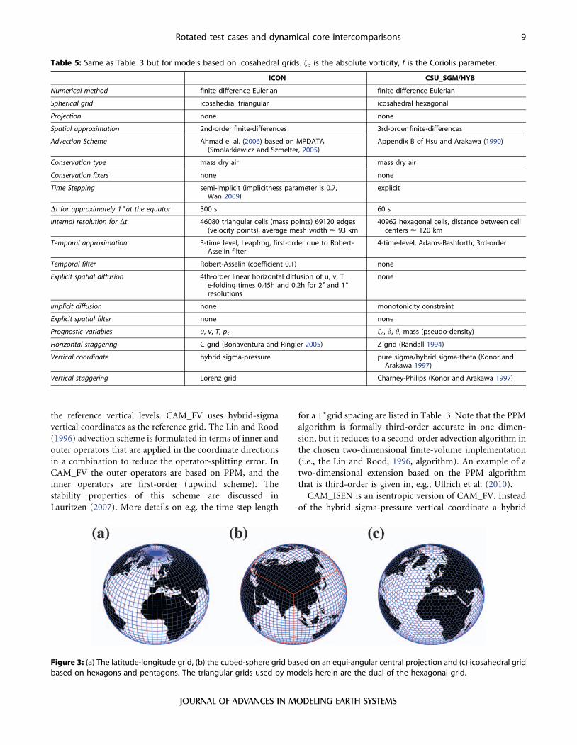
Figure 3: (a) The latitude-longitude grid, (b) the cubed-sphere grid based on an equi-angular central projection and (c) icosahedral gridbased on hexagons and pentagons. The triangular grids used by models herein are the dual of the hexagonal grid.
Rotated test cases and dynamical core intercomparisons 9
JOURNAL OF ADVANCES IN MODELING EARTH SYSTEMS
sigma-h vertical coordinate is used (Chen and Rasch 2010).
Apart from the vertical coordinate the model design is
identical to CAM_FV.
3.2. Cubed-sphere grid models
The assessment includes two dynamical cores that are
defined on cubed-sphere grids. The finite-volume cubed-
sphere model (GEOS_FV_CUBED) is a cubed-sphere ver-
sion of CAM_FV developed at the Geophysical Fluid
Dynamics Laboratory (GFDL) and the NASA Goddard
Space Flight Center. The advection scheme is based on the
Lin and Rood (1996) method but adapted to non-ortho-
gonal cubed-sphere grids (Putman and Lin 2007, 2009). Like
CAM_FV, the GEOS_FV_CUBED dynamical core is sec-
ond-order accurate in two dimensions. Both a weak second-
order divergence damping mechanism and an additional
fourth-order divergence damping scheme is used with
coefficients 0.005 6 DAmin/Dt and [0.05 6 DAmin]2/Dt,
respectively, where DAmin is the smallest grid cell area in the
domain.
The strength of the divergence damping increases towards
the model top to define a 3-layer sponge. In contrast to
CAM_FV and CAM_ISEN, the cubed-sphere model does
not apply any digital or FFT filtering in the polar regions
and mid-latitudes. Nevertheless, an external-mode filter is
implemented that damps the horizontal momentum equa-
tions. This is accomplished by adding the external-mode
damping coefficient (0.02 6 DAmin/Dt) times the gradient
of the vertically-integrated horizontal divergence on the
right-hand-side of the vector momentum equation.
GEOS_FV_CUBED applies the same inner and outer
operators in the advection scheme (PPM) to avoid the
inconsistencies described in Lauritzen (2007) when using
different orders of inner and outer operators. The cubed-
sphere grid is based on central angles. The angles are chosen
to form an equal-distance grid at the cubed-sphere edges
(undocumented). The equal-distance grid is similar to an
equidistant cubed-sphere grid that is explained in Nair et al.
(2005). The resolution is specified in terms of the number of
cells along a panel side. As an example, 90 cells along each
side of a cubed-sphere face yield a global grid spacing of
about 1 .
The second cubed-sphere dynamical core is NCAR’s
spectral element High-Order Method Modeling Environ-
ment (HOMME) (Thomas and Loft 2005, Nair et al. 2009).
Spectral elements are a type of a continuous-Galerkin h-p
finite element method (Karniadakis and Sherwin 1999,
Canuto et al. 2007), where h is the number of elements
and p the polynomial order. Rather than using cell averages
as prognostic variables as in geos_fv_cubed, the finite
element method uses p-order polynomials to represent the
prognostic variables inside each element. The spectral ele-
ment method is compatible, meaning it has discrete analogs of
the key integral properties of the divergence, gradient and
curl operators, making the method elementwise mass-
conservative (to machine precision) and total energy conser-
vative (to the truncation error of the time-integration
scheme) (Taylor et al. 2007, Taylor et al. 2008). The cubed-
sphere grid consists of elements with boundaries defined by
an equiangular gnomonic grid (Nair et al. 2005) and each
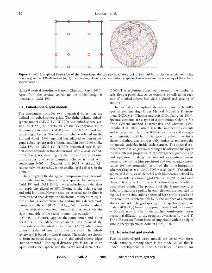
element has (p + 1) 6 (p + 1) Gauss-Legendre-Lobatto
quadrature points. The positions of the Gauss-Legendre-
Lobatto quadrature points in each element are depicted in
Fig. 4. For the simulations presented here p 5 3 is used and
the resolution is determined by h, the number of elements
along a face side. The grid spacing at the equator is approxi-
mately 90 /(h 1 p) hence the approximately 1˚solutions use h
5 30 and p 5 3. The model applies fourth-order linear
horizontal diffusion to the prognostic variables u, v and T.
The diffusion coefficient is tuned empirically with the help of
kinetic energy spectra as done in CAM_EUL.
3.3. Icosahedral grid models
Two icosahedral-grid based models are tested with three
model variants. Among them is the model ICON that is
under development at the Max-Planck Institute for
Figure 4: (left) A graphical illustration of the Gauss-Legendre-Lobatto quadrature points (red unfilled circles) in an element (blueboundary) of the HOMME model. (right) The mapping of every element onto the sphere. Green lines are the boundary of the cubed-sphere faces.
10 Lauritzen et al.
JAMES Vol. 2 2010 adv-model-earth-syst.org
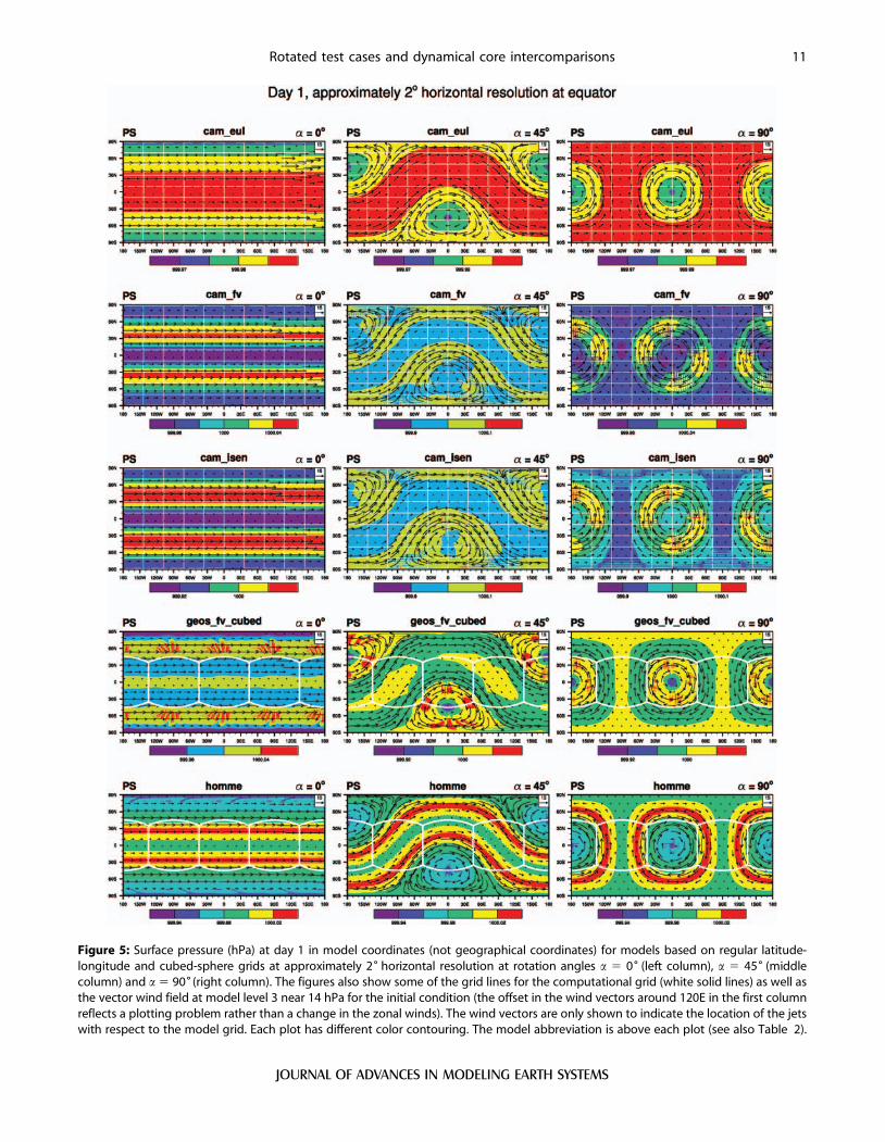
Figure 5: Surface pressure (hPa) at day 1 in model coordinates (not geographical coordinates) for models based on regular latitude-longitude and cubed-sphere grids at approximately 2˚ horizontal resolution at rotation angles a 5 0˚ (left column), a 5 45˚ (middlecolumn) and a 5 90˚(right column). The figures also show some of the grid lines for the computational grid (white solid lines) as well asthe vector wind field at model level 3 near 14 hPa for the initial condition (the offset in the wind vectors around 120E in the first columnreflects a plotting problem rather than a change in the zonal winds). The wind vectors are only shown to indicate the location of the jetswith respect to the model grid. Each plot has different color contouring. The model abbreviation is above each plot (see also Table 2).
Rotated test cases and dynamical core intercomparisons 11
JOURNAL OF ADVANCES IN MODELING EARTH SYSTEMS
Meteorology, Germany, and the German Weather Service
DWD. Some documentation on ICON is given in Wan
(2009). The second model labeled CSU has been developed
at the Colorado State University, Fort Collins, U.S.. Here
two model variant of CSU are assessed that use different
vertical coordinates. The icosahedral grids are special types
of geodesic grids where an icosahedron inscribed in a sphere
is subdivided recursively to form a quasi-uniform grid of
triangles. In the CSU model the grid resolution is specified
in terms of the number of refinement levels of the icosahed-
ron that initially consists of 20 triangles. Each refinement
level subdivides the mesh, thereby doubling its resolution.
The hexagonal grid is the dual of the triangular grid. It is
created by connecting the centroids of the triangles sharing a
vertex with great circle arcs. It consists primarily of hexa-
gons and 12 pentagons. If , is the number of bisections of an
original icosahedral edge the number of hexagonal grid cells
is given by
2z10|4‘: ð3:2Þ
A resolution of approximately 1˚ is obtained with , 5 6
(40962 cells) corresponding to a minimum and maximum
grid point distance between the cell centers of 110 km and
132 km, respectively. The number of triangles in this grid is
given by
20|4‘ ð3:3Þ
which corresponds to 81920 triangles for , 5 6. Note that
the ICON results discussed in this paper are based on a
slightly different distribution of the triangular grid cells. The
main difference is the initial refinement strategy for the
icosahedron. Instead of bisecting the grid, the original
icosahedron is first split by a factor of three along each edge
before further recursive bisections are introduced. If m 5 , -
2 5 4 is the number of bisections after the initial 3-way split
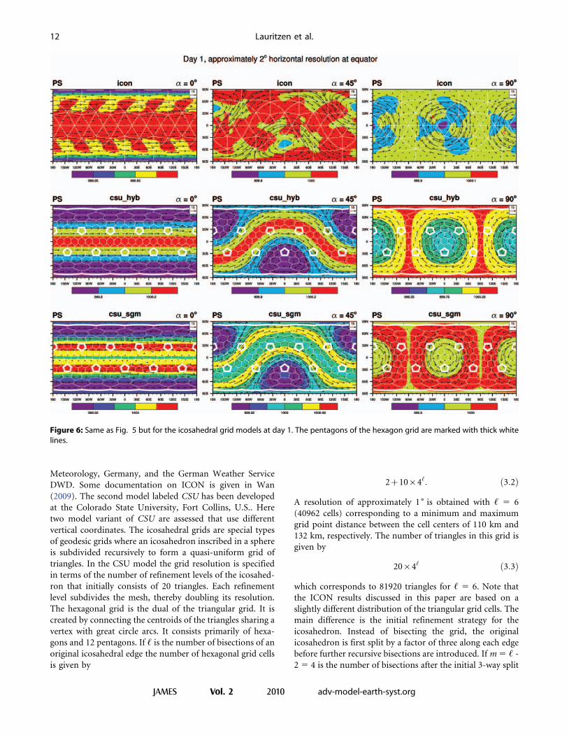
Figure 6: Same as Fig. 5 but for the icosahedral grid models at day 1. The pentagons of the hexagon grid are marked with thick whitelines.
12 Lauritzen et al.
JAMES Vol. 2 2010 adv-model-earth-syst.org
the number of triangular cells nc, triangle edges ne and
triangle vertices nv is then given by
nc~20|32|4m ð3:4Þ
ne~30|32|4m ð3:5Þ
nv~10|32|4mz2: ð3:6Þ
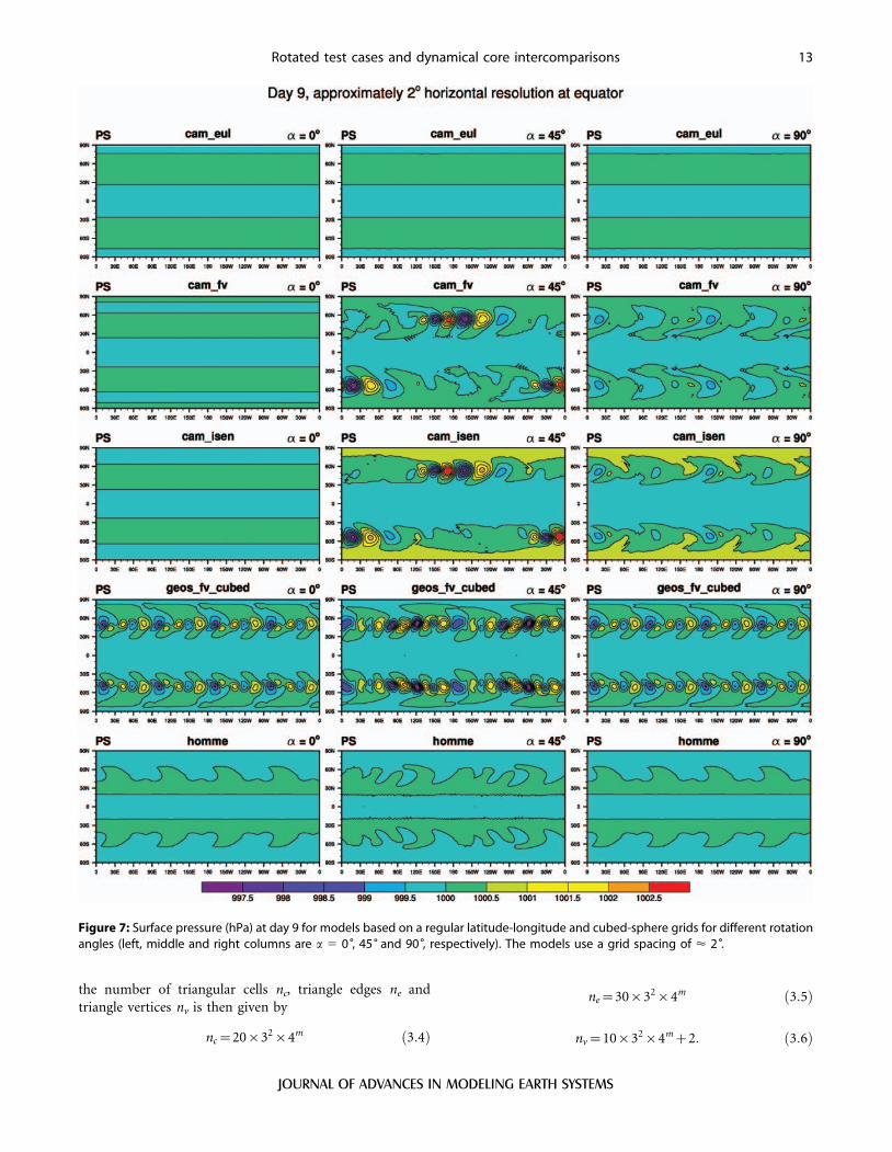
Figure 7: Surface pressure (hPa) at day 9 for models based on a regular latitude-longitude and cubed-sphere grids for different rotationangles (left, middle and right columns are a 5 0 , 45˚ and 90 , respectively). The models use a grid spacing of < 2 .
Rotated test cases and dynamical core intercomparisons 13
JOURNAL OF ADVANCES IN MODELING EARTH SYSTEMS
For the approximately 1˚ triangular grid with m 5 4, 46080
triangular cells with 69120 edges and 23042 vertices result in an
average mesh width of 93 km. One can either use the hexagons
(pentagons) or triangles as control volumes for the discretiza-
tion. The icosahedral grids give an almost homogeneous and
quasi-isotropic coverage of the sphere. The hexagonal grid has
a somewhat higher degree of symmetry than triangular grids
whereas triangular grids are more straight forward to refine if
mesh refinement is desired. Both icosahedral grid models
(CSU and ICON) optimize the icosahedral grid so that the
truncation error for the spatial finite-difference operators is
guaranteed to converge to zero as the grid-cell sizes decrease to
zero. See Heikes and Randall (1995) for more details.
In this study, we use a development version of the ICON
(Icosahedral Nonhydrostatic) dynamical core that utilizes
the triangular control volumes. Although the model abbre-
viation refers to a non-hydrostatic model, the version used
here is based on the hydrostatic equation set in vector-
invariant form. The model applies 2nd-order finite-differ-
ence approximations on an Arakawa C horizontal grid
(Bonaventura and Ringler 2005) and a Lorenz grid in the
vertical. The velocity reconstruction algorithm is based on
Radial Basis Functions (RBF). The vertical coordinate is the
hybrid sigma-pressure coordinate. The time-stepping algo-
rithm is semi-implicit using an implicitness parameter of 0.7
(see Wan 2009). The computational mode of the three-
time-level Leapfrog time-stepping scheme is damped with a
Robert-Asselin filter. The advection scheme is MPDATA
(Smolarkiewicz 1983; Smolarkiewicz and Szmelter 2005)
adapted to the icosahedral grid (Ahmad el al. 2006).
Efforts are ongoing to develop a higher-order advection
scheme for ICON (A. Gassman, personal communication
2009). Fourth-order linear horizontal diffusion is applied to
u, v, T along the model levels. The time steps used for the 1˚(46080 cells) and 2˚ (11520 cells) runs are 300 s and 600 s,
respectively. It should be noted that the ICON model is
undergoing rapid development (partly due to the experience
with the test case suite run during the NCAR ASP 2008
summer colloquium). Hence, the results presented here are
with an older version of ICON.
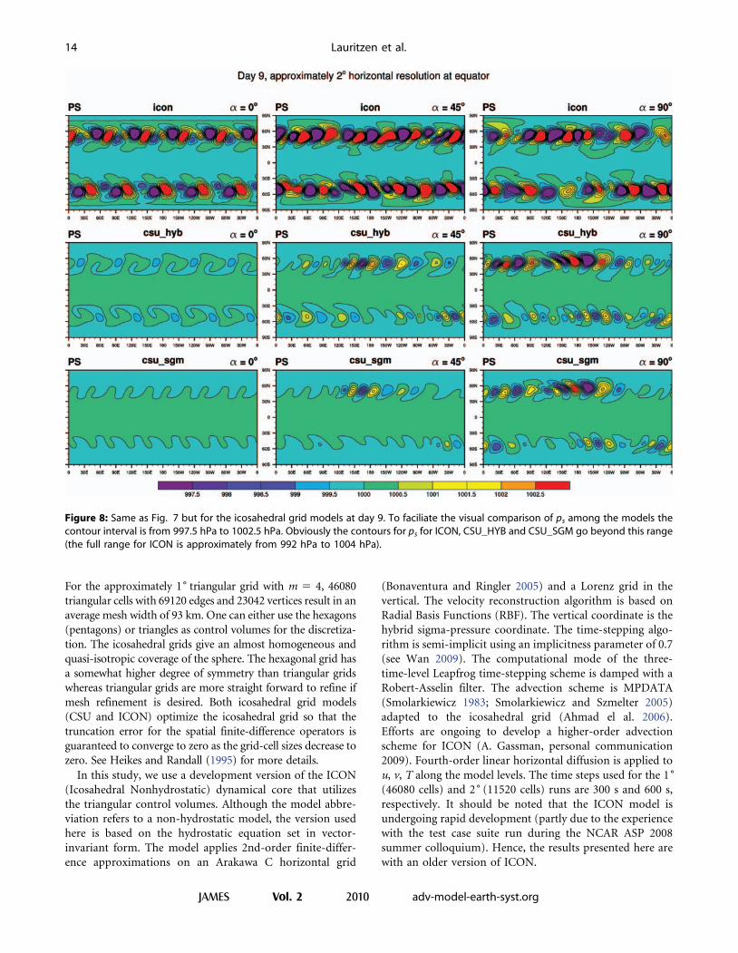
Figure 8: Same as Fig. 7 but for the icosahedral grid models at day 9. To faciliate the visual comparison of ps among the models thecontour interval is from 997.5 hPa to 1002.5 hPa. Obviously the contours for ps for ICON, CSU_HYB and CSU_SGM go beyond this range(the full range for ICON is approximately from 992 hPa to 1004 hPa).
14 Lauritzen et al.
JAMES Vol. 2 2010 adv-model-earth-syst.org
The CSU dynamical core is based on hexagons (and 12
pentagons). The model directly predicts vorticity and
divergence. Stream function and velocity potential are
obtained by solving elliptic equations using multigrid
methods. The vorticity and divergence are co-located at
cell centers following the Z-grid (Randall 1994) that pro-
vides attractive linear dispersion properties for, e.g., geo-
strophic adjustment and has no computational modes.
A four-time-level third-order Adams-Bashforth time-
integration method is used for mass (pseudo-density), h,
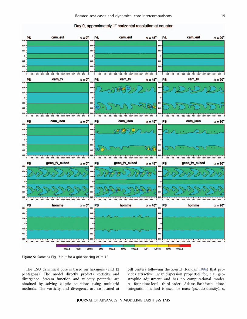
Figure 9: Same as Fig. 7 but for a grid spacing of < 1 .
Rotated test cases and dynamical core intercomparisons 15
JOURNAL OF ADVANCES IN MODELING EARTH SYSTEMS
absolute vorticity fa, and divergence d. The advection
scheme of the CSU model is described in Appendix B of
Hsu and Arakawa (1990). Two options for the vertical
coordinates are used in these tests. One is the traditional
pure sigma coordinate (CSU_SGM) while the other is a
hybrid sigma-theta vertical coordinate (Konor and Arakawa
1997) referred to as CSU_HYB. The vertical staggering is an
equivalent Charney-Philips staggering (Konor and Arakawa
1997). Monotonicity constraints in the advection operator
(flux-corrected transport, Zalesak 1979) may produce
implicit diffusion. The time steps for the 1˚ (40962 cells)
and 2˚ (10242 cells) grid spacings are 60 s and 120 s,
respectively.
4. Results
To facilitate data handling and model comparisons the
output for each model was interpolated to a regular lat-
itude-longitude grid. In the model HOMME the interpola-
tion was performed by evaluating the internal basis
functions at the regular latitude-longitude grid points.
CSU_SGM and CSU_HYB use area-weighted interpolation
and GEOS_FV_CUBED use bilinear interpolation. For the
baroclinic wave test case, the ,2-error for a particular model
are computed by interpolating the non-rotated high-resolu-
tion reference solution (CAM_EUL at T340 resolution) to
the regular latitude-longitude grid to which the native
model data has been interpolated.
4.1. Rotated steady-state test case
The steady-state test case measures the model’s ability to
maintain a steady-state solution and its sensitivity to the
rotation of the grid while keeping the physical flow the
same. For simplicity the test is evaluated in terms of the
surface pressure field which avoids vertical interpolations to
pressure levels. No new insights are found when assessing
other variables like T, u, v, f, d. Figure 5 shows the ps field in
model coordinates (not geographical coordinates) at day 1
for models based on regular latitude-longitude and cubed-
sphere grids with the approximately 2˚ horizontal resolu-
tion. The figures also show some of the grid lines of the
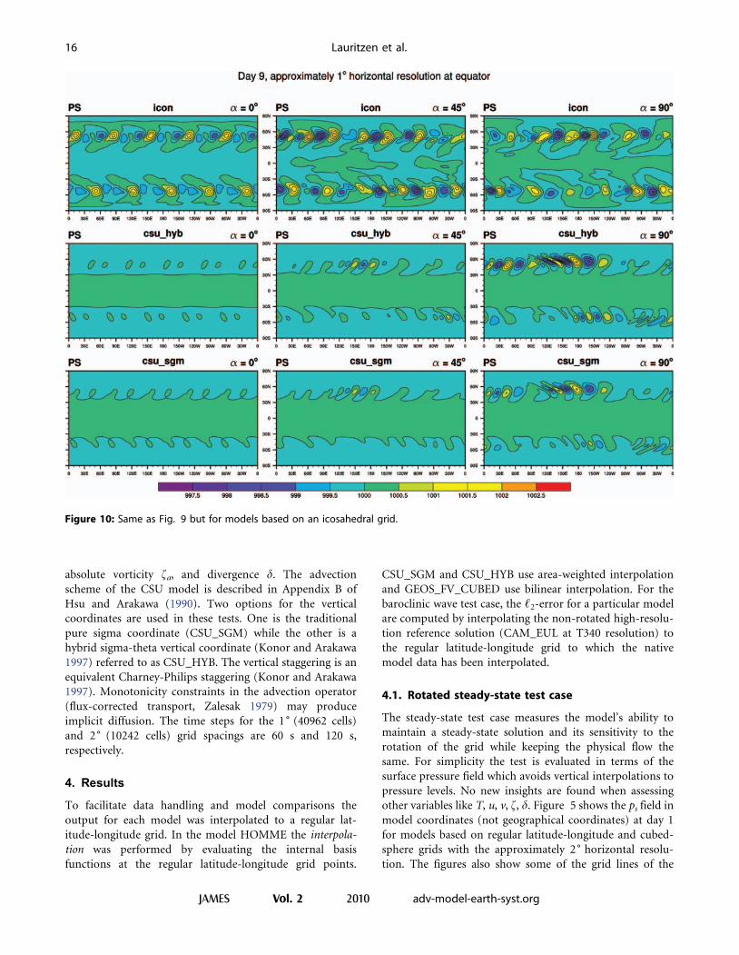
Figure 10: Same as Fig. 9 but for models based on an icosahedral grid.
16 Lauritzen et al.
JAMES Vol. 2 2010 adv-model-earth-syst.org
computational grid as well as selected wind vectors at model
level 3 near 14 hPa. The wind vectors show the locations of
the jets in the model’s coordinate system. The computa-
tional grid lines illustrate how the grid impacts the numer-
ical solution (discussed separately below for each model).
Note that the contours for ps are not the same for all plots.
Figure 6 is the same as Fig. 5 but for the icosahedral-grid
based models.
In addition to model day 1 we also show the surface
pressure fields at day 9 when the grid effects are more
pronounced. Model day 9 is depicted in Figs. 7 and 9 that
show the dynamical cores based on regular latitude-longit-
ude and cubed-sphere grids at approximately 2˚ and 1˚horizontal resolutions, respectively. A common contour
interval is used. Results for the icosahedral grid models
are presented in Figs. 8 and 10. The steady-state test has
an analytic solution (ps 5 1000 hPa) that allows the
computation of root mean square ,2 error. The ,2 error
for the regular latitude-longitude and cubed-sphere grids are
shown in Fig. 11. Figure 12 depicts the time series of the
surface pressure error for the icosahedral-hexagonal models.
The definition of the ,2-error is provided in JW06. Each
figure is discussed in greater detail below.
The three-dimensional steady-state flow is baroclinically
and barotropically unstable due to its horizontal and vertical
shear characteristics, hence any perturbation introduced
into the flow will grow. Due to the basic mechanisms in
baroclinic instability the flow is more sensitive to perturba-
tions introduced around the midlatitudes near the latitud-
inal position of the jets in contrast to, for example,
perturbations introduced at the equator.
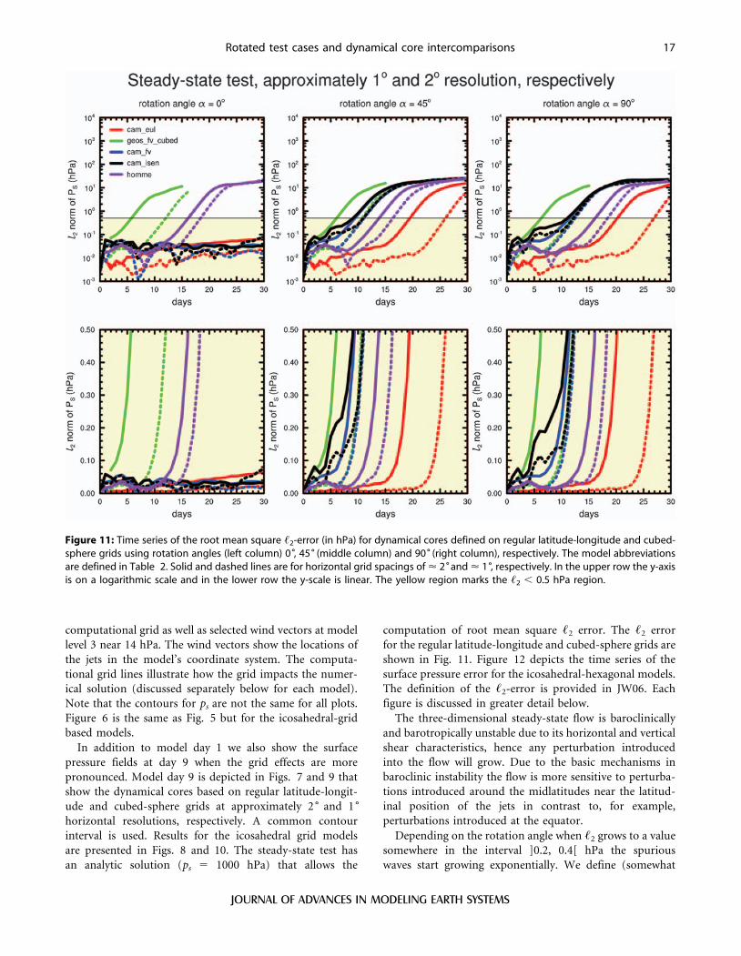
Depending on the rotation angle when ,2 grows to a value
somewhere in the interval ]0.2, 0.4[ hPa the spurious
waves start growing exponentially. We define (somewhat
Figure 11: Time series of the root mean square ,2-error (in hPa) for dynamical cores defined on regular latitude-longitude and cubed-sphere grids using rotation angles (left column) 0 , 45˚(middle column) and 90˚(right column), respectively. The model abbreviationsare defined in Table 2. Solid and dashed lines are for horizontal grid spacings of < 2˚and < 1 , respectively. In the upper row the y-axisis on a logarithmic scale and in the lower row the y-scale is linear. The yellow region marks the ,2 , 0.5 hPa region.
Rotated test cases and dynamical core intercomparisons 17
JOURNAL OF ADVANCES IN MODELING EARTH SYSTEMS
arbitrarily) ,2 5 0.5 hPa as the threshold value after which a
model is termed unable to maintain a balanced flow. At that
point the amplitude of the spurious waves has grown
beyond approximately 0.5 hPa and grows exponentially.
Note that the same conclusions could be drawn by using
any threshold value larger than approximately 0.3 hPa (and
less than approximately 8 hPa).
4.1.1. Regular latitude-longitude grid modelsThe unrotated results of the regular latitude-longitude
models show that the numerical schemes maintain the
balances in the flow for at least 30 days (left column in
Fig. 11). However, when the computational grid is rotated
so that the flow is no longer aligned with the grid lines,
spurious waves start growing early during the simulation. In
case of CAM_FV and CAM_ISEN (Fig. 5) noisy patterns
appear in the surface pressure fields by day 1. The spurious
waves have larger amplitudes for a 5 45˚ than for a 5 90 .
For a 5 45˚the jets cross the poles of the computational grid
(Fig. 1). Numerical approximations near the poles such as
filtering, averaging, etc., trigger a wave train in each
hemisphere similar to the wave train triggered by the
boundaries in the limited-area model of Lauritzen et al.
(2008). In their case however, the growing wave was
triggered by the boundary relaxation scheme and elliptic
solver in the boundary zone.
For a 5 90˚ the poles of the computational grid are at the
equator and hence far away from the baroclinically most
unstable region located in the mid-latitudes. Hence less
accurate approximations in the polar regions of the com-
putational grid are not the main trigger for spurious waves
rather the fact that the grid lines predominantly are at an
angle with respect to the jets (see, e.g., Fig. 1). In fact the
angle between the jet maximum and the computation grid
latitudes is approximately 45˚ in four locations and less than
45˚ elsewhere. The numerical approximations tend to be
most accurate for flow aligned with grid lines (angle between
jet and computational latitudes < 0 ) and least accurate for
traverse flow (angle between jet and computational latitudes
< 45 ). This seems to trigger the wavenumber four pattern
apparent in the surface pressure fields of the two finite
volume models at day 9 (Fig. 7, right column).
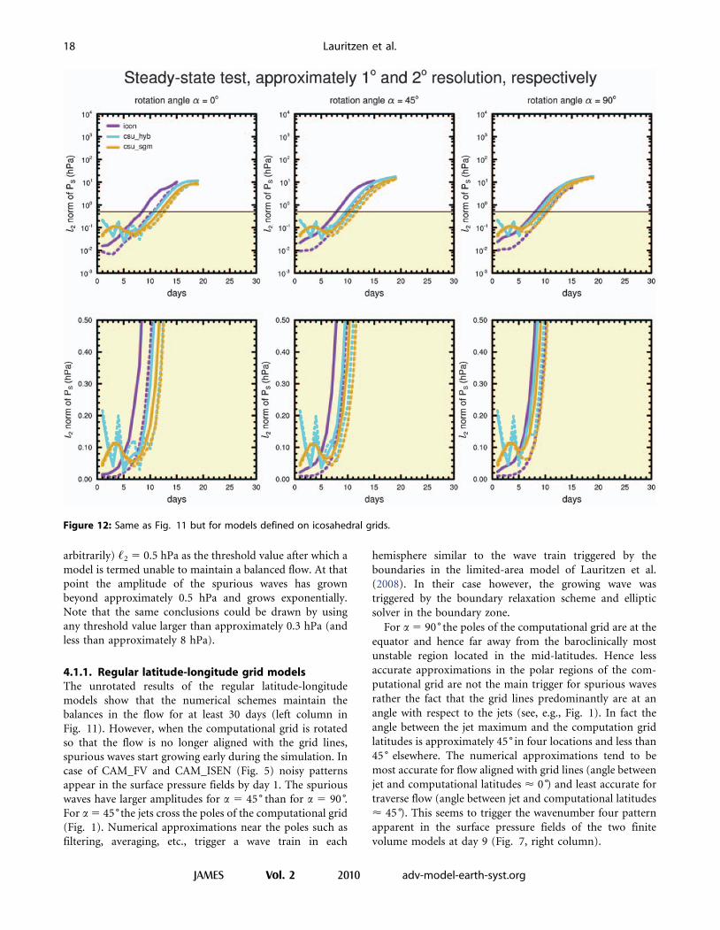
Figure 12: Same as Fig. 11 but for models defined on icosahedral grids.
18 Lauritzen et al.
JAMES Vol. 2 2010 adv-model-earth-syst.org
The growth of the baroclinic wave is slightly stronger in
CAM_ISEN than in CAM_FV. When doubling the hori-
zontal resolution similar results are obtained (Figs. 7 and
9). Nevertheless, the growth of the spurious waves is delayed
by approximately two days (Fig. 11) at the higher resolu-
tion. This is expected since higher resolutions reduce the
numerical truncation errors.
For CAM_EUL the results at day 9 at low and high
resolutions (Figs. 7 and 9) appear to be invariant under
rotation. This might be expected due to the fact that a
triangular truncation of spherical harmonics is invariant
under rotation. However, the ,2-error in Fig. 11 reveal that
the rotated versions of CAM_EUL cannot maintain a
balanced initial state throughout the 30-day integration.
At about day 19 and 26 the rotated versions of CAM_EUL
lose the symmetry at the 2˚ and 1˚ resolutions, respectively.
It is speculated that the spurious wave is triggered because
the spherical harmonic functions do not represent the initial
conditions exactly.
4.1.2. Cubed-sphere models
Both cubed-sphere models HOMME and
GEOS_FV_CUBED show a distinct wavenumber 4 grid
imprint in the surface pressure field at day 9 at the coarse
2˚ resolution (Fig. 7, last two rows). The grid imprint
appears in each hemisphere for a 5 0˚ and a 5 90 . The
corners of the cubed-sphere in each hemisphere are located
near the centers of the jets for a 5 0˚ and a 5 90 , thereby
positioning them in the baroclinically most unstable
regions. This is depicted in Fig. 5 that shows the cubed-
sphere panel-side outline and the position of the jets. The
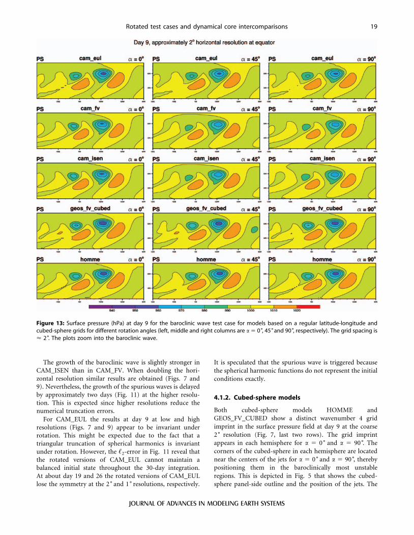
Figure 13: Surface pressure (hPa) at day 9 for the baroclinic wave test case for models based on a regular latitude-longitude andcubed-sphere grids for different rotation angles (left, middle and right columns are a 5 0 , 45˚and 90 , respectively). The grid spacing is< 2 . The plots zoom into the baroclinic wave.
Rotated test cases and dynamical core intercomparisons 19
JOURNAL OF ADVANCES IN MODELING EARTH SYSTEMS
discretizations tend to have the largest errors near the
corners of the inscribed cube. Since these are near the
baroclinically most unstable regions, the wavenumber 4
spurious wave is induced into the circulation and grows
fast. The amplitude of the spurious wave is larger in
GEOS_FV_CUBED than in HOMME. This is most likely
due to the high-order numerical scheme and consistent
finite-element-based treatment of the corners in HOMME.
There is some indication that the Putman and Lin (2007)
advection scheme introduces additional errors, in particular
near the edges, due to its dimensional split characteristics as
explained in the next paragraph.
In the challenging moving vortices advection test case of
Nair and Jablonowski (2008) the convergence rates for the
Lauritzen et al. (2010) scheme is approximately one order of
magnitude higher than for the Putman and Lin (2007)
scheme. Both schemes use the same order of reconstruction
function so the only major difference between the two
schemes is that the Lauritzen et al. (2010) scheme is fully
two-dimensional, in particular it uses a rigorous fully two-
dimensional treatment of the corners of the cube, whereas
the Putman and Lin (2007) scheme uses a dimensional split
approach. This seems to indicate that the dimensional split
approach has a less accurate treatment of the corners of the
cubed-sphere as compared to other approaches.
GEOS_FV_CUBED can no longer maintain the steady-
state at approximately day 6 and 12 for the 2˚ and 1˚resolution (Fig. 11). Hence, doubling the horizontal resolu-
tion delays the break-down of the steady-state by 6 days
which is a large improvement compared to most other
models. This could indicate that GEOS_FV_CUBED is
below its minimal recommendable resolution at a 2˚ grid
spacing. The model HOMME can maintain the steady-state
for 16 and 18 days at the coarse and fine resolutions.
In the a 5 45˚ case (Fig. 11, middle column) we observe
that the performance of the models degrade and the break-
down of the steady-states occurs approximately 2 days
earlier in comparison to a 5 0 , 90˚ (apart from
GEOS_FV_CUBED at 2˚ resolution). The wave signature
in the surface pressure field has an overlaid wavenumber 2
and wavenumber 4 characteristic rather than a pure wave-
number 4 imprint as seen before (Figs. 7 and 9). The
following reasons are suggested. At the a 5 45˚ rotation
angle the flanks of the jets traverse two vertices rather than
four (Fig. 5). This triggers the wavenumber 2 error sig-
nature that overlays the wavenumber 4 background error. In
addition, the advection operators tend to be more accurate
when the flow is quasi-parallel to coordinate lines which is
predominantly the case for a 5 0˚ and a 5 90 . At the a 5
45˚ rotation angle the flow mostly traverse the coordinate
lines at an angle, thereby triggering enhanced errors as also
discussed in Lauritzen (2007).
4.1.3. Icosahedral models
Similar to the corners of the cubed-sphere grid and the
pole points of the regular latitude-longitude mesh, the
hexagonal-icosahdral grids have 12 pentagons that usually
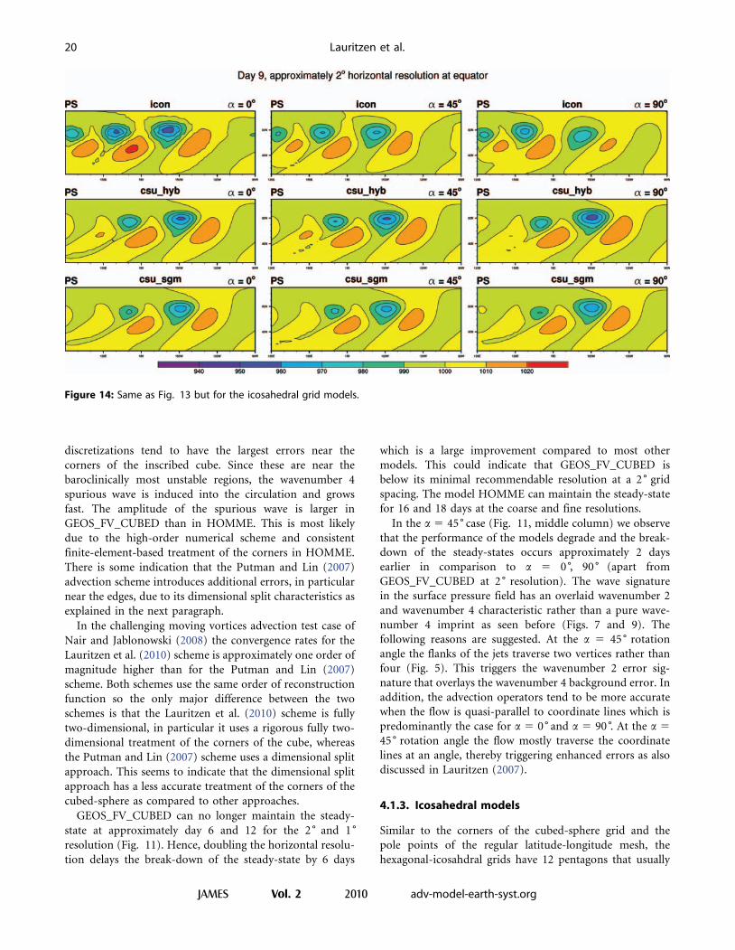
Figure 14: Same as Fig. 13 but for the icosahedral grid models.
20 Lauritzen et al.
JAMES Vol. 2 2010 adv-model-earth-syst.org
require special attention in the model discretizations. The
triangular-hexagonal grids show the largest deviations
from their almost uniform grid spacings near the dual-
grid pentagons. This triggers a distinct and expected
wavenumber 5 grid imprint in the icosahedral-grid based
models in the non-rotated case (Fig. 8). The spurious
wave trains in the Northern and Southern atmosphere
are offset by 36˚ degrees due to the relative location of the
pentagons in the two hemispheres (Fig. 8 and 10). Note
that the pentagons are located near the maximum intensity
of the jets (Fig. 6) where the flow is baroclinically most
unstable. The model ICON already shows the wavenumber
5 pattern at day 1.
In the rotated cases it is less clear how the numerical
discretizations near the pentagons adversely affect the solu-
tion. For a 5 45˚and a 5 90˚the locations of the pentagons
in each hemisphere of the computational domain are
not symmetric since (regular) hexagons have symmetry
properties for 60˚ rather than 45˚ and 90 . This triggers
the asymmetric response in the surface pressure field in all
icosahedral simulations at the rotation angles a 5 45˚ and
90˚ (Fig. 8 and 10, middle and right column). At the 1˚resolution (Fig. 10) the amplitudes of the growing spurious
waves in ICON are largest at the a 5 45˚ rotation angle,
whereas they are largest at the 90˚ angle in the models
CSU_HYB and CSU_SGM. All three icosahedral model
variants improve their representation of the steady-state at
the higher resolution. The ICON model can maintain the
steady-state solution the shortest. It breaks down after
approximately 8 and 10 days at the 2˚ and 1˚ resolutions,
respectively. The steady-states in the high-resolution ver-
sions of CSU_SGM and CSU_HYB break down after
approximately 12 days whereas the lower resolution version
differs by a day (Fig. 12). The CSU_HYB model variant
with the hybrid isentropic vertical coordinate shows that the
spurious perturbations introduced by the numerics grow
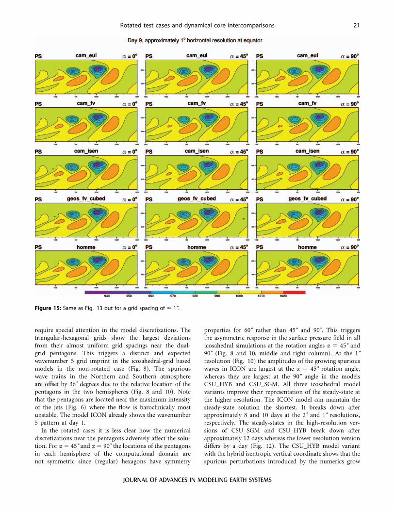
Figure 15: Same as Fig. 13 but for a grid spacing of < 1 .
Rotated test cases and dynamical core intercomparisons 21
JOURNAL OF ADVANCES IN MODELING EARTH SYSTEMS
slightly faster than the perturbations in the traditional
sigma-pressure model version. A similar observation was
made for the CAM_FV and CAM_ISEN model pair.
4.2. Rotated baroclinic wave test case
As for the steady-state test case we consider the surface
pressure at day 9 with three rotation angles (a 5 0 , 45 ,
90 ) and the two 2˚and 1˚resolutions. The figures for surface
pressure are grouped as before for the steady-state test case. In
particular, the surface pressure field at the low resolution for
the regular latitude-longitude and cubed-sphere grid based
models are shown in Fig. 13. The icosahedral-grid based
models are depicted in Fig. 14. The plots zoom in on the
main wave train in the northern hemisphere. The corres-
ponding plots for the high 1˚resolution runs are presented in
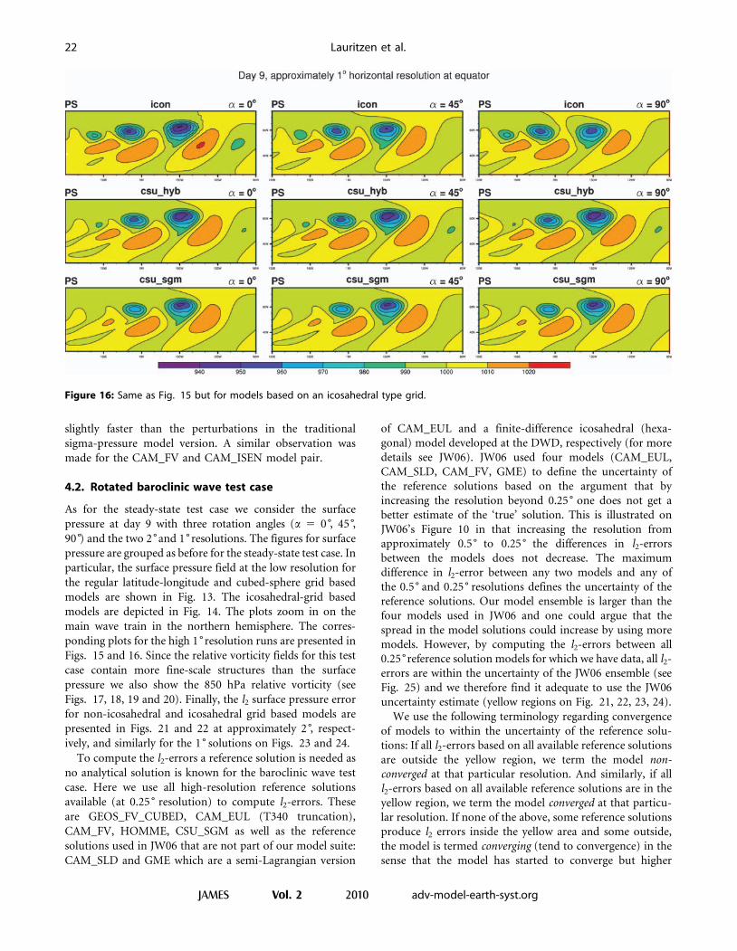
Figs. 15 and 16. Since the relative vorticity fields for this test
case contain more fine-scale structures than the surface
pressure we also show the 850 hPa relative vorticity (see
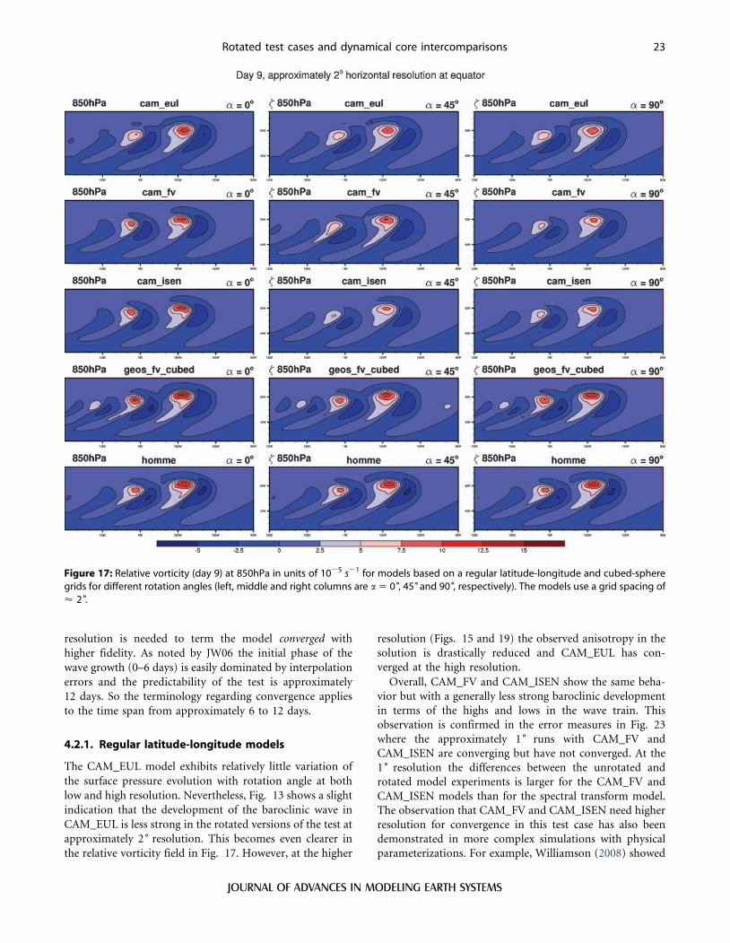
Figs. 17, 18, 19 and 20). Finally, the l2 surface pressure error
for non-icosahedral and icosahedral grid based models are
presented in Figs. 21 and 22 at approximately 2 , respect-
ively, and similarly for the 1˚ solutions on Figs. 23 and 24.
To compute the l2-errors a reference solution is needed as
no analytical solution is known for the baroclinic wave test
case. Here we use all high-resolution reference solutions
available (at 0.25˚ resolution) to compute l2-errors. These
are GEOS_FV_CUBED, CAM_EUL (T340 truncation),
CAM_FV, HOMME, CSU_SGM as well as the reference
solutions used in JW06 that are not part of our model suite:
CAM_SLD and GME which are a semi-Lagrangian version
of CAM_EUL and a finite-difference icosahedral (hexa-
gonal) model developed at the DWD, respectively (for more
details see JW06). JW06 used four models (CAM_EUL,
CAM_SLD, CAM_FV, GME) to define the uncertainty of
the reference solutions based on the argument that by
increasing the resolution beyond 0.25˚ one does not get a
better estimate of the ‘true’ solution. This is illustrated on
JW06’s Figure 10 in that increasing the resolution from
approximately 0.5˚ to 0.25˚ the differences in l2-errors
between the models does not decrease. The maximum
difference in l2-error between any two models and any of
the 0.5˚ and 0.25˚ resolutions defines the uncertainty of the
reference solutions. Our model ensemble is larger than the
four models used in JW06 and one could argue that the
spread in the model solutions could increase by using more
models. However, by computing the l2-errors between all
0.25˚reference solution models for which we have data, all l2-
errors are within the uncertainty of the JW06 ensemble (see
Fig. 25) and we therefore find it adequate to use the JW06
uncertainty estimate (yellow regions on Fig. 21, 22, 23, 24).
We use the following terminology regarding convergence
of models to within the uncertainty of the reference solu-
tions: If all l2-errors based on all available reference solutions
are outside the yellow region, we term the model non-
converged at that particular resolution. And similarly, if all
l2-errors based on all available reference solutions are in the
yellow region, we term the model converged at that particu-
lar resolution. If none of the above, some reference solutions
produce l2 errors inside the yellow area and some outside,
the model is termed converging (tend to convergence) in the
sense that the model has started to converge but higher
Figure 16: Same as Fig. 15 but for models based on an icosahedral type grid.
22 Lauritzen et al.
JAMES Vol. 2 2010 adv-model-earth-syst.org
resolution is needed to term the model converged with
higher fidelity. As noted by JW06 the initial phase of the
wave growth (0–6 days) is easily dominated by interpolation
errors and the predictability of the test is approximately
12 days. So the terminology regarding convergence applies
to the time span from approximately 6 to 12 days.
4.2.1. Regular latitude-longitude models
The CAM_EUL model exhibits relatively little variation of
the surface pressure evolution with rotation angle at both
low and high resolution. Nevertheless, Fig. 13 shows a slight
indication that the development of the baroclinic wave in
CAM_EUL is less strong in the rotated versions of the test at
approximately 2˚ resolution. This becomes even clearer in
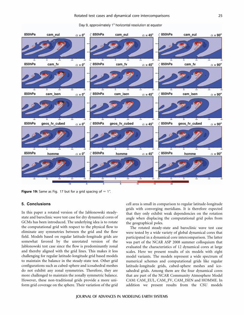
the relative vorticity field in Fig. 17. However, at the higher
resolution (Figs. 15 and 19) the observed anisotropy in the
solution is drastically reduced and CAM_EUL has con-
verged at the high resolution.
Overall, CAM_FV and CAM_ISEN show the same beha-
vior but with a generally less strong baroclinic development
in terms of the highs and lows in the wave train. This
observation is confirmed in the error measures in Fig. 23
where the approximately 1˚ runs with CAM_FV and
CAM_ISEN are converging but have not converged. At the
1˚ resolution the differences between the unrotated and
rotated model experiments is larger for the CAM_FV and
CAM_ISEN models than for the spectral transform model.
The observation that CAM_FV and CAM_ISEN need higher
resolution for convergence in this test case has also been
demonstrated in more complex simulations with physical
parameterizations. For example, Williamson (2008) showed
Figure 17: Relative vorticity (day 9) at 850hPa in units of 1025 s21 for models based on a regular latitude-longitude and cubed-spheregrids for different rotation angles (left, middle and right columns are a 5 0 , 45˚and 90 , respectively). The models use a grid spacing of< 2 .
Rotated test cases and dynamical core intercomparisons 23
JOURNAL OF ADVANCES IN MODELING EARTH SYSTEMS
in so-called aqua-planet experiments (Neale and Hoskins
2000) that CAM_FV needs a higher horizontal resolution to
match the CAM_EUL results in terms of a wide range of
diagnostics.
4.2.2. Cubed-sphere models
The cubed-sphere models perform very similarly and show
little dependence on rotation angle. At the approximately 2˚resolution the deep low in surface pressure at day 9 is
slightly deeper for the rotated cubed-sphere runs than for
the corresponding CAM_EUL run (Fig. 13). At high res-
olution CAM_EUL and the cubed-sphere models show
almost identical ps fields (Fig. 15). This indicates that the
cubed-sphere models have converged as is confirmed in the
l2 error measures in Fig. 23. There is a slight indication in
the l2 error that for a 5 45˚ the solutions are slightly less
accurate than for the other rotation angles. In fact
GEOS_FV_CUBED at a 5 45˚ is on the verge to be termed
converging rather than converged. Also, the relative vorticity
fields show some slight variation with rotation angle at both
low and high resolution for the cubed-sphere models
(Fig. 17 and 19). This is most likely due to the flow being
predominantly traverse to grid cells at a 5 45 . In contrast
the flow is predominantly parallel to the grid lines for a 5 0˚and a 5 90 .
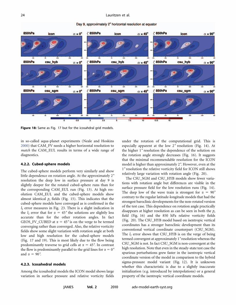
4.2.3. Icosahedral models
Among the icosahedral models the ICON model shows large
variation in surface pressure and relative vorticity fields
under the rotation of the computational grid. This is
especially apparent at the low 2˚ resolution (Fig. 14). At
the higher 1˚ resolution the dependence of the solution on
the rotation angle strongly decreases (Fig. 16). It suggests
that the minimal recommendable resolution for the ICON
model is higher than approximately 2 . However, even at the
1˚ resolution the relative vorticity field for ICON still shows
relatively large variation with rotation angle (Fig. 20).
The CSU_SGM and CSU_HYB models show fewer varia-
tions with rotation angle but differences are visible in the
surface pressure field for the low resolution runs (Fig. 14).
The deep low of the wave train is strongest for a 5 90˚contrary to the regular latitude-longitude models that had the
strongest baroclinic developments for the non-rotated version
of the test case. This dependence on rotation angle practically
disappears at higher resolution as can be seen in both the ps
field (Fig. 16) and the 850 hPa relative vorticity fields
(Fig. 20). The CSU_HYB model based on isentropic vertical
coordinates has a stronger baroclinic development than its
conventional vertical coordinate counterpart (CSU_SGM).
The l2 error shows that CSU_HYB is on the verge of being
termed convergent at approximately 1˚resolution whereas the
CSU_SGM is not. In fact CSU_SGM is non-convergent at the
high resolution. Note that even in the steady-state test case the
spurious perturbations grew faster in the isentropic vertical
coordinate version of the model in comparison to the hybrid
sigma-pressure model variant (Fig. 12). It is unknown
whether this characteristic is due to a slightly inaccurate
initialization (e.g. introduced by interpolations) or a general
property of the isentropic vertical coordinate models.
Figure 18: Same as Fig. 17 but for the icosahdral grid models.
24 Lauritzen et al.
JAMES Vol. 2 2010 adv-model-earth-syst.org
5. Conclusions
In this paper a rotated version of the Jablonowski steady-
state and baroclinic wave test case for dry dynamical cores of
GCMs has been introduced. The underlying idea is to rotate
the computational grid with respect to the physical flow to
eliminate any symmetries between the grid and the flow
field. Models based on regular latitude-longitude grids are
somewhat favored by the unrotated version of the
Jablonowski test case since the flow is predominantly zonal
and thereby aligned with the grid lines. This makes it less
challenging for regular latitude-longitude grid based models
to maintain the balance in the steady-state test. Other grid
configurations such as cubed-sphere and icosahedral meshes
do not exhibit any zonal symmetries. Therefore, they are
more challenged to maintain the zonally symmetric balance.
However, these non-traditional grids provide a more uni-
form grid coverage on the sphere. Their variation of the grid
cell area is small in comparison to regular latitude-longitude
grids with converging meridians. It is therefore expected
that they only exhibit weak dependencies on the rotation
angle when displacing the computational grid poles from
the geographical poles.
The rotated steady-state and baroclinic wave test case
were tested by a wide variety of global dynamical cores that
participated in a dynamical core intercomparison. The latter
was part of the NCAR ASP 2008 summer colloquium that
evaluated the characteristics of 12 dynamical cores at large
scales. Here we present results of six models with eight
model variants. The models represent a wide spectrum of
numerical schemes and computational grids like regular
latitude-longitude grids, cubed-sphere meshes and ico-
sahedral grids. Among them are the four dynamical cores
that are part of the NCAR Community Atmosphere Model
CAM: CAM_EUL, CAM_FV, CAM_ISEN and HOMME. In
addition we present results from the CSU models
Figure 19: Same as Fig. 17 but for a grid spacing of < 1 .
Rotated test cases and dynamical core intercomparisons 25
JOURNAL OF ADVANCES IN MODELING EARTH SYSTEMS
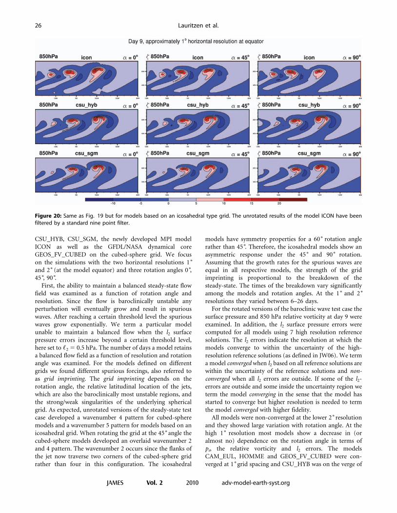
CSU_HYB, CSU_SGM, the newly developed MPI model
ICON as well as the GFDL/NASA dynamical core
GEOS_FV_CUBED on the cubed-sphere grid. We focus
on the simulations with the two horizontal resolutions 1˚and 2˚ (at the model equator) and three rotation angles 0 ,
45 , 90 .
First, the ability to maintain a balanced steady-state flow
field was examined as a function of rotation angle and
resolution. Since the flow is baroclinically unstable any
perturbation will eventually grow and result in spurious
waves. After reaching a certain threshold level the spurious
waves grow exponentially. We term a particular model
unable to maintain a balanced flow when the l2 surface
pressure errors increase beyond a certain threshold level,
here set to ,2 5 0.5 hPa. The number of days a model retains
a balanced flow field as a function of resolution and rotation
angle was examined. For the models defined on different
grids we found different spurious forcings, also referred to
as grid imprinting. The grid imprinting depends on the
rotation angle, the relative latitudinal location of the jets,
which are also the baroclinically most unstable regions, and
the strong/weak singularities of the underlying spherical
grid. As expected, unrotated versions of the steady-state test
case developed a wavenumber 4 pattern for cubed-sphere
models and a wavenumber 5 pattern for models based on an
icosahedral grid. When rotating the grid at the 45˚ angle the
cubed-sphere models developed an overlaid wavenumber 2
and 4 pattern. The wavenumber 2 occurs since the flanks of
the jet now traverse two corners of the cubed-sphere grid
rather than four in this configuration. The icosahedral
models have symmetry properties for a 60˚ rotation angle
rather than 45 . Therefore, the icosahedral models show an
asymmetric response under the 45˚ and 90˚ rotation.
Assuming that the growth rates for the spurious waves are
equal in all respective models, the strength of the grid
imprinting is proportional to the breakdown of the
steady-state. The times of the breakdown vary significantly
among the models and rotation angles. At the 1˚ and 2˚resolutions they varied between 6–26 days.
For the rotated versions of the baroclinic wave test case the
surface pressure and 850 hPa relative vorticity at day 9 were
examined. In addition, the l2 surface pressure errors were
computed for all models using 7 high resolution reference
solutions. The l2 errors indicate the resolution at which the
models converge to within the uncertainty of the high-
resolution reference solutions (as defined in JW06). We term
a model converged when l2 based on all reference solutions are
within the uncertainty of the reference solutions and non-
converged when all l2 errors are outside. If some of the l2-
errors are outside and some inside the uncertainty region we
term the model converging in the sense that the model has
started to converge but higher resolution is needed to term
the model converged with higher fidelity.
All models were non-converged at the lower 2˚ resolution
and they showed large variation with rotation angle. At the
high 1˚ resolution most models show a decrease in (or
almost no) dependence on the rotation angle in terms of
ps, the relative vorticity and l2 errors. The models
CAM_EUL, HOMME and GEOS_FV_CUBED were con-
verged at 1˚grid spacing and CSU_HYB was on the verge of
Figure 20: Same as Fig. 19 but for models based on an icosahedral type grid. The unrotated results of the model ICON have beenfiltered by a standard nine point filter.
26 Lauritzen et al.
JAMES Vol. 2 2010 adv-model-earth-syst.org
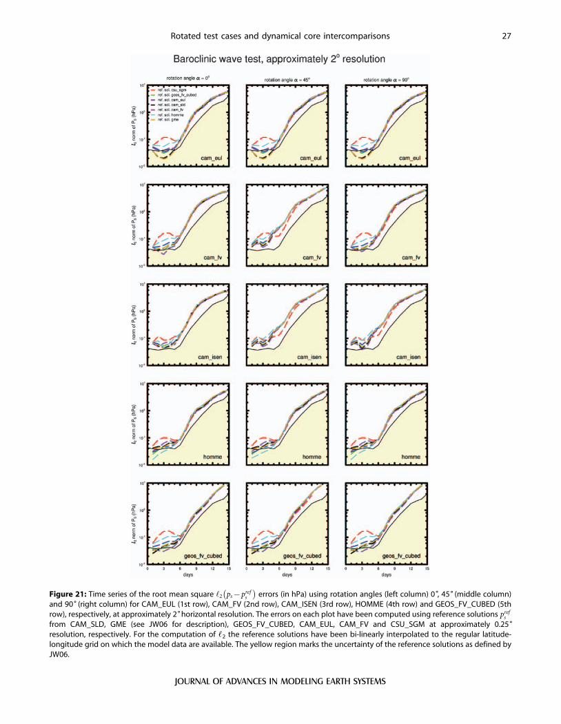
Figure 21: Time series of the root mean square ‘2 ps{prefs
� errors (in hPa) using rotation angles (left column) 0 , 45˚(middle column)
and 90˚(right column) for CAM_EUL (1st row), CAM_FV (2nd row), CAM_ISEN (3rd row), HOMME (4th row) and GEOS_FV_CUBED (5throw), respectively, at approximately 2˚horizontal resolution. The errors on each plot have been computed using reference solutions pref
s
from CAM_SLD, GME (see JW06 for description), GEOS_FV_CUBED, CAM_EUL, CAM_FV and CSU_SGM at approximately 0.25˚resolution, respectively. For the computation of ,2 the reference solutions have been bi-linearly interpolated to the regular latitude-longitude grid on which the model data are available. The yellow region marks the uncertainty of the reference solutions as defined byJW06.
Rotated test cases and dynamical core intercomparisons 27
JOURNAL OF ADVANCES IN MODELING EARTH SYSTEMS
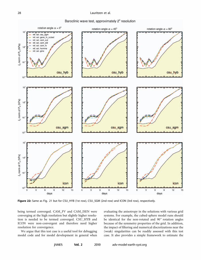
being termed converged. CAM_FV and CAM_ISEN were
converging at the high resolution but slightly higher resolu-
tion is needed to be termed converged. CSU_HYB and
ICON were non-convergent and therefore need higher
resolution for convergence.
We argue that this test case is a useful tool for debugging
model code and for model development in general when
evaluating the anisotropy in the solutions with various grid
systems. For example, the cubed-sphere model runs should
be identical for the non-rotated and 90˚ rotation angles
because of the symmetry properties of the grid. In addition,
the impact of filtering and numerical discretizations near the
(weak) singularities can be readily assessed with this test
case. It also provides a simple framework to estimate the
Figure 22: Same as Fig. 21 but for CSU_HYB (1st row), CSU_SGM (2nd row) and ICON (3rd row), respectively.
28 Lauritzen et al.
JAMES Vol. 2 2010 adv-model-earth-syst.org
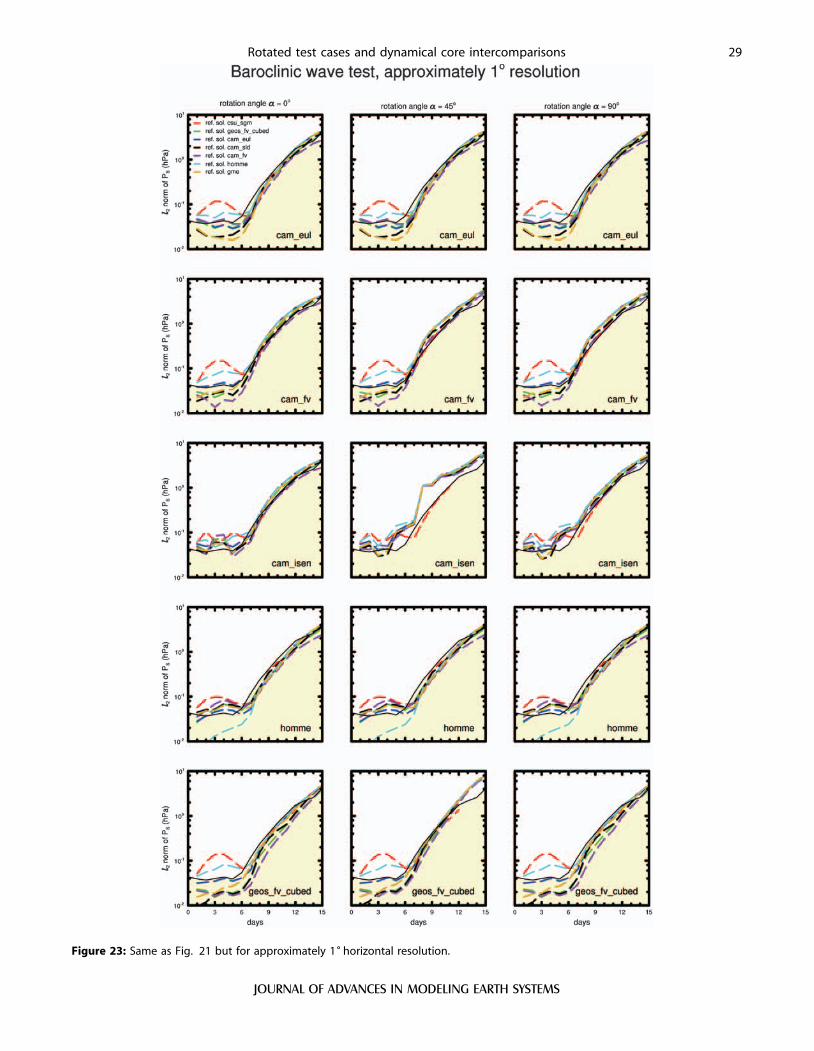
Figure 23: Same as Fig. 21 but for approximately 1˚ horizontal resolution.
Rotated test cases and dynamical core intercomparisons 29
JOURNAL OF ADVANCES IN MODELING EARTH SYSTEMS
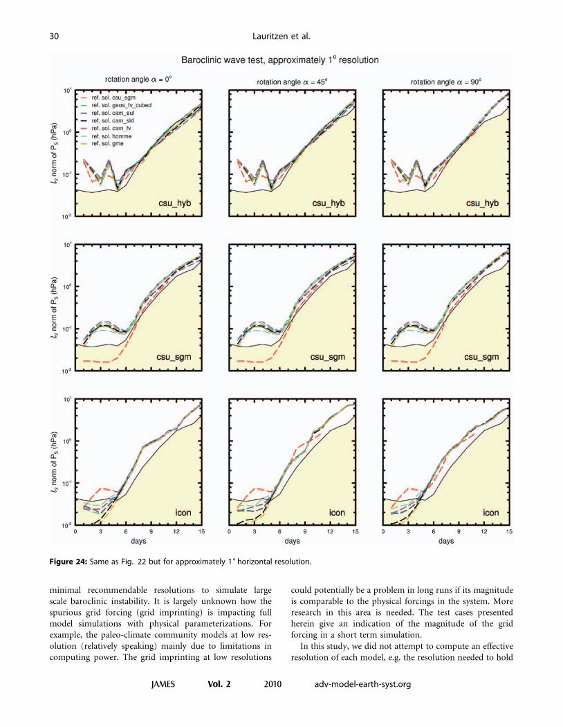
minimal recommendable resolutions to simulate large
scale baroclinic instability. It is largely unknown how the
spurious grid forcing (grid imprinting) is impacting full
model simulations with physical parameterizations. For
example, the paleo-climate community models at low res-
olution (relatively speaking) mainly due to limitations in
computing power. The grid imprinting at low resolutions
could potentially be a problem in long runs if its magnitude
is comparable to the physical forcings in the system. More
research in this area is needed. The test cases presented
herein give an indication of the magnitude of the grid
forcing in a short term simulation.
In this study, we did not attempt to compute an effective
resolution of each model, e.g. the resolution needed to hold
Figure 24: Same as Fig. 22 but for approximately 1˚ horizontal resolution.
30 Lauritzen et al.
JAMES Vol. 2 2010 adv-model-earth-syst.org
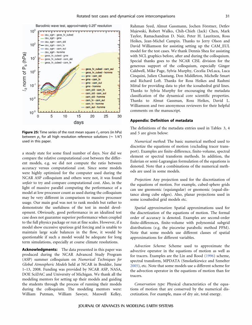
a steady state for some fixed number of days. Nor did we
compare the relative computational cost between the differ-
ent models, e.g. we did not compute the ratio between
accuracy versus computational cost. Since some models
were highly optimized for the computer used during the
NCAR ASP colloquium and others were not, it was found
unfair to try and compare computational cost. Also, in the
light of massive parallel computing the performance of a
model at low processor count as used during the colloquium
may be very different in comparison to massive processor
usage. Our main goal was not to rank models but rather to
demonstrate the usefulness of the test in model devel-
opment. Obviously, good performance in an idealized test
case does not guarantee superior performance when coupled
to the full physics package or run at fine scales. However, if a
model show excessive spurious grid forcing and is unable to
maintain large scale balances in the flow, it would be
questionable if such a model would be adequate for long
term simulations, especially at coarse climate resolutions.
Acknowledgments: The data presented in this paper was
produced during the NCAR Advanced Study Program
(ASP) summer colloquium on Numerical Techniques for
Global Atmospheric Models held at NCAR in Boulder, June
1–13, 2008. Funding was provided by NCAR ASP, NASA,
DOE SciDAC and University of Michigan. We thank all the
modeling mentors for setting up their models and guiding
the students through the process of running their models
during the colloquium. The modeling mentors were:
William Putman, William Sawyer, Maxwell Kelley,
Rahman Syed, Almut Gassmann, Jochen Forstner, Detlev
Majewski, Robert Walko, Chih-Chieh (Jack) Chen, Mark
Taylor, Ramachandran D. Nair, Peter H. Lauritzen, Ross
Heikes, Jean-Michel Campin. Thanks to Jerry Olson and
David Williamson for assisting setting up the CAM_EUL
model for the test cases. We thank Dennis Shea for assisting
with NCL graphics before, after and during the colloquium.
Special thanks goes to the NCAR CISL division for the
generous support of the colloquium, especially Ginger
Caldwell, Mike Page, Sylvia Murphy, Cecelia DeLuca, Luca
Cinquini, Julien Chastang, Don Middleton, Michelle Smart
and Richard Loft. Thanks for Ross Heikes and Rashmi
Mittal for providing data to plot the icosahedral grid lines.
Thanks to Sylvia Murphy for encouraging the metadata
classification of the dynamical core scientific properties.
Thanks to Almut Gassman, Ross Heikes, David L.
Williamson and two anonymous reviewers for their helpful
comments on the manuscript.
Appendix: Definition of metadata
The definitions of the metadata entries used in Tables 3, 4
and 5 are given below:
Numerical method: The basic numerical method used to
discretize the equations of motion (excluding tracer trans-
port). Examples are finite-difference, finite-volume, spectral
element or spectral transform methods. In addition, the
Eulerian or semi-Lagrangian formulation of the equations is
denoted. Note that a combinations of the numerical meth-
ods are used in some models.
Projection: Any projection used for the discretization of
the equations of motion. For example, cubed-sphere grids
can use gnomonic (equiangular) or gnomonic (equal-dis-
tance along cube edges). Also, planar projections used in
some icosahedral grid models etc.
Spatial approximation: Spatial approximations used for
the discretization of the equations of motion. The formal
order of accuracy is denoted. Examples are second-order
finite-differences, finite-volume with polynomial subgrid
distributions (e.g. the piecewise parabolic method PPM).
Note that some models use different classes of spatial
approximations for different variables.
Advection Scheme: Scheme used to approximate the
advective operator in the equations of motion as well as
for tracers. Examples are the Lin and Rood (1996) scheme,
spectral transform, MPDATA (Smolarkiewicz and Szmelter
2005), etc. Note that some models use a different scheme for
the advection operator in the equations of motion than for
tracers.
Conservation type: Physical characteristics of the equa-
tions of motion that are conserved by the numerical dis-
cretization. For example, mass of dry air, total energy.
Figure 25: Time series of the root mean square ,2 errors (in hPa)between ps for all high resolution reference solutions (< 1/4 )used in this paper.
Rotated test cases and dynamical core intercomparisons 31
JOURNAL OF ADVANCES IN MODELING EARTH SYSTEMS
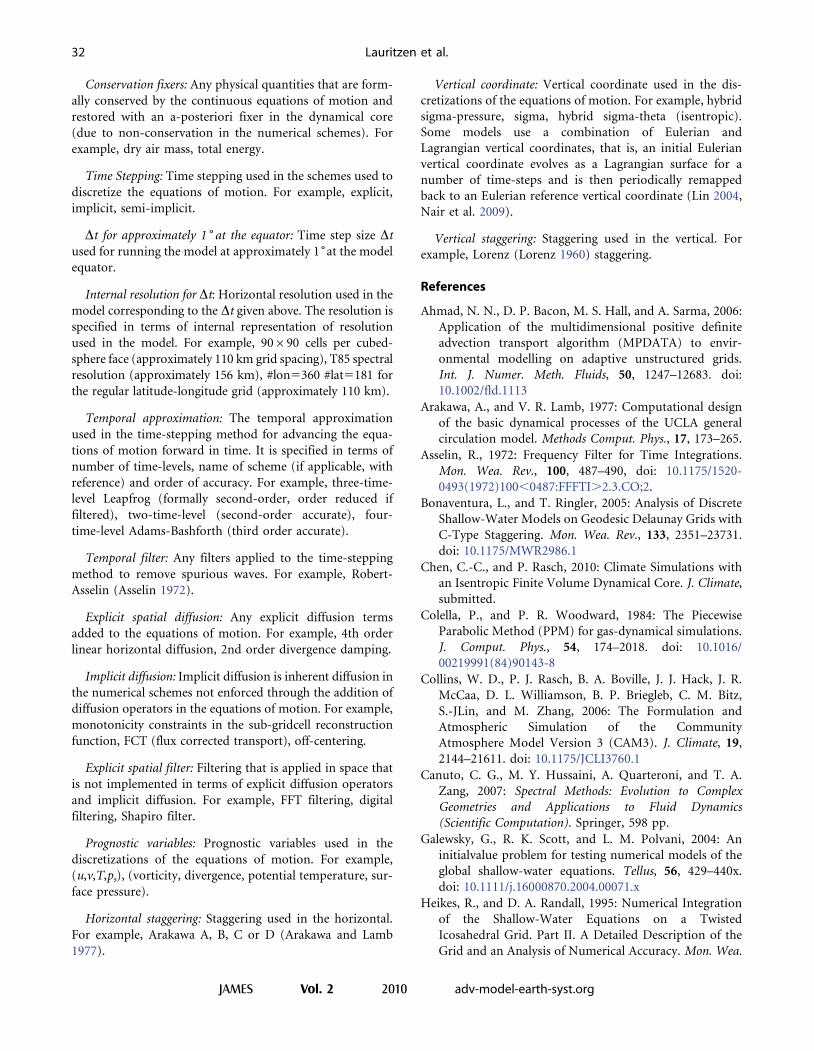
Conservation fixers: Any physical quantities that are form-
ally conserved by the continuous equations of motion and
restored with an a-posteriori fixer in the dynamical core
(due to non-conservation in the numerical schemes). For
example, dry air mass, total energy.
Time Stepping: Time stepping used in the schemes used to
discretize the equations of motion. For example, explicit,
implicit, semi-implicit.
Dt for approximately 1˚ at the equator: Time step size Dt
used for running the model at approximately 1˚at the model
equator.
Internal resolution for Dt: Horizontal resolution used in the
model corresponding to the Dt given above. The resolution is
specified in terms of internal representation of resolution
used in the model. For example, 90690 cells per cubed-
sphere face (approximately 110 km grid spacing), T85 spectral
resolution (approximately 156 km), #lon5360 #lat5181 for
the regular latitude-longitude grid (approximately 110 km).
Temporal approximation: The temporal approximation
used in the time-stepping method for advancing the equa-
tions of motion forward in time. It is specified in terms of
number of time-levels, name of scheme (if applicable, with
reference) and order of accuracy. For example, three-time-
level Leapfrog (formally second-order, order reduced if
filtered), two-time-level (second-order accurate), four-
time-level Adams-Bashforth (third order accurate).
Temporal filter: Any filters applied to the time-stepping
method to remove spurious waves. For example, Robert-
Asselin (Asselin 1972).
Explicit spatial diffusion: Any explicit diffusion terms
added to the equations of motion. For example, 4th order
linear horizontal diffusion, 2nd order divergence damping.
Implicit diffusion: Implicit diffusion is inherent diffusion in
the numerical schemes not enforced through the addition of
diffusion operators in the equations of motion. For example,
monotonicity constraints in the sub-gridcell reconstruction
function, FCT (flux corrected transport), off-centering.
Explicit spatial filter: Filtering that is applied in space that
is not implemented in terms of explicit diffusion operators
and implicit diffusion. For example, FFT filtering, digital
filtering, Shapiro filter.
Prognostic variables: Prognostic variables used in the
discretizations of the equations of motion. For example,
(u,v,T,ps), (vorticity, divergence, potential temperature, sur-
face pressure).
Horizontal staggering: Staggering used in the horizontal.
For example, Arakawa A, B, C or D (Arakawa and Lamb
1977).
Vertical coordinate: Vertical coordinate used in the dis-
cretizations of the equations of motion. For example, hybrid
sigma-pressure, sigma, hybrid sigma-theta (isentropic).
Some models use a combination of Eulerian and
Lagrangian vertical coordinates, that is, an initial Eulerian
vertical coordinate evolves as a Lagrangian surface for a
number of time-steps and is then periodically remapped
back to an Eulerian reference vertical coordinate (Lin 2004,
Nair et al. 2009).
Vertical staggering: Staggering used in the vertical. For
example, Lorenz (Lorenz 1960) staggering.
References
Ahmad, N. N., D. P. Bacon, M. S. Hall, and A. Sarma, 2006:
Application of the multidimensional positive definite
advection transport algorithm (MPDATA) to envir-
onmental modelling on adaptive unstructured grids.
Int. J. Numer. Meth. Fluids, 50, 1247–12683. doi:
10.1002/fld.1113
Arakawa, A., and V. R. Lamb, 1977: Computational design
of the basic dynamical processes of the UCLA general
circulation model. Methods Comput. Phys., 17, 173–265.
Asselin, R., 1972: Frequency Filter for Time Integrations.
Mon. Wea. Rev., 100, 487–490, doi: 10.1175/1520-
0493(1972)100,0487:FFFTI.2.3.CO;2.
Bonaventura, L., and T. Ringler, 2005: Analysis of Discrete
Shallow-Water Models on Geodesic Delaunay Grids with
C-Type Staggering. Mon. Wea. Rev., 133, 2351–23731.
doi: 10.1175/MWR2986.1
Chen, C.-C., and P. Rasch, 2010: Climate Simulations with
an Isentropic Finite Volume Dynamical Core. J. Climate,
submitted.
Colella, P., and P. R. Woodward, 1984: The Piecewise
Parabolic Method (PPM) for gas-dynamical simulations.
J. Comput. Phys., 54, 174–2018. doi: 10.1016/
00219991(84)90143-8
Collins, W. D., P. J. Rasch, B. A. Boville, J. J. Hack, J. R.
McCaa, D. L. Williamson, B. P. Briegleb, C. M. Bitz,
S.-JLin, and M. Zhang, 2006: The Formulation and
Atmospheric Simulation of the Community
Atmosphere Model Version 3 (CAM3). J. Climate, 19,
2144–21611. doi: 10.1175/JCLI3760.1
Canuto, C. G., M. Y. Hussaini, A. Quarteroni, and T. A.
Zang, 2007: Spectral Methods: Evolution to Complex
Geometries and Applications to Fluid Dynamics
(Scientific Computation). Springer, 598 pp.
Galewsky, G., R. K. Scott, and L. M. Polvani, 2004: An
initialvalue problem for testing numerical models of the
global shallow-water equations. Tellus, 56, 429–440x.
doi: 10.1111/j.16000870.2004.00071.x
Heikes, R., and D. A. Randall, 1995: Numerical Integration
of the Shallow-Water Equations on a Twisted
Icosahedral Grid. Part II. A Detailed Description of the
Grid and an Analysis of Numerical Accuracy. Mon. Wea.
32 Lauritzen et al.
JAMES Vol. 2 2010 adv-model-earth-syst.org
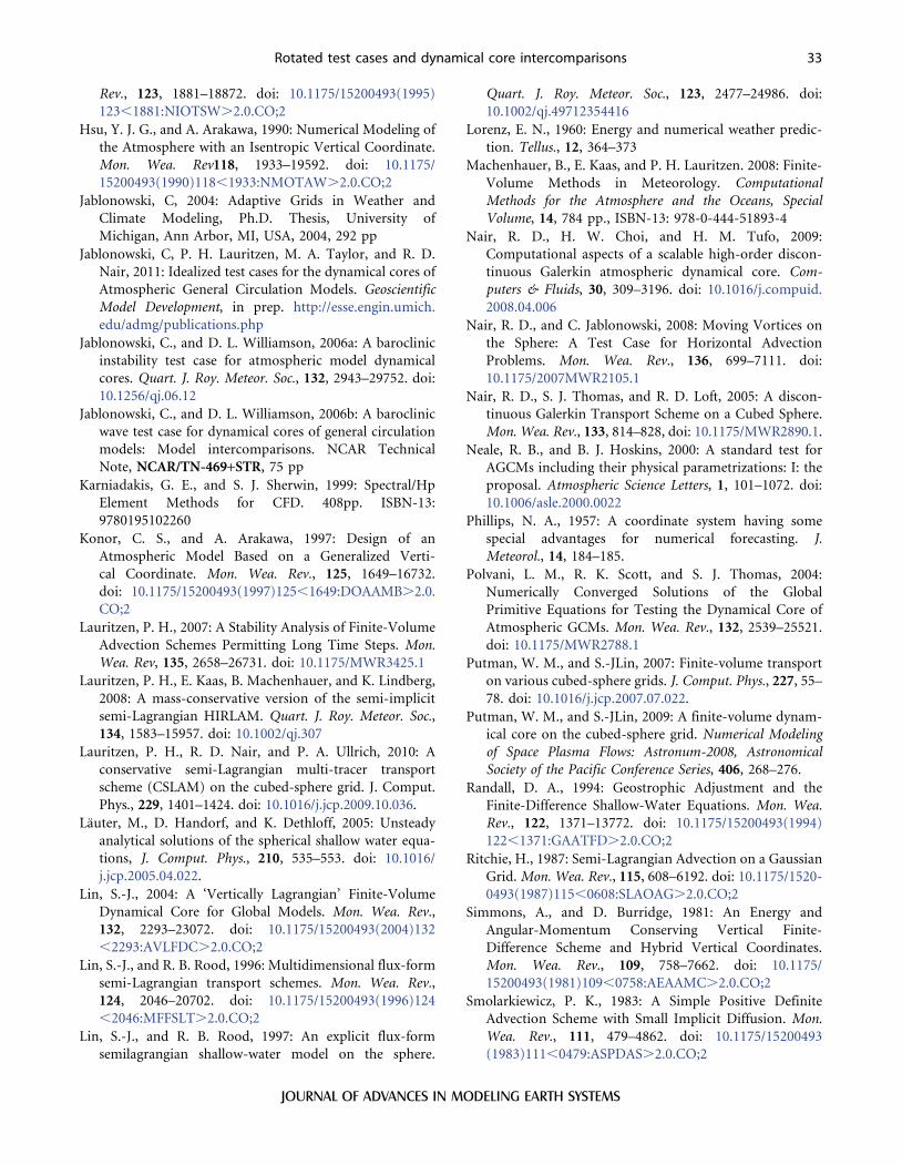
Rev., 123, 1881–18872. doi: 10.1175/15200493(1995)
123,1881:NIOTSW.2.0.CO;2
Hsu, Y. J. G., and A. Arakawa, 1990: Numerical Modeling of
the Atmosphere with an Isentropic Vertical Coordinate.
Mon. Wea. Rev118, 1933–19592. doi: 10.1175/
15200493(1990)118,1933:NMOTAW.2.0.CO;2
Jablonowski, C, 2004: Adaptive Grids in Weather and
Climate Modeling, Ph.D. Thesis, University of
Michigan, Ann Arbor, MI, USA, 2004, 292 pp
Jablonowski, C, P. H. Lauritzen, M. A. Taylor, and R. D.
Nair, 2011: Idealized test cases for the dynamical cores of
Atmospheric General Circulation Models. Geoscientific
Model Development, in prep. http://esse.engin.umich.
edu/admg/publications.php
Jablonowski, C., and D. L. Williamson, 2006a: A baroclinic
instability test case for atmospheric model dynamical
cores. Quart. J. Roy. Meteor. Soc., 132, 2943–29752. doi:
10.1256/qj.06.12
Jablonowski, C., and D. L. Williamson, 2006b: A baroclinic
wave test case for dynamical cores of general circulation
models: Model intercomparisons. NCAR Technical
Note, NCAR/TN-469+STR, 75 pp
Karniadakis, G. E., and S. J. Sherwin, 1999: Spectral/Hp
Element Methods for CFD. 408pp. ISBN-13:
9780195102260
Konor, C. S., and A. Arakawa, 1997: Design of an
Atmospheric Model Based on a Generalized Verti-
cal Coordinate. Mon. Wea. Rev., 125, 1649–16732.
doi: 10.1175/15200493(1997)125,1649:DOAAMB.2.0.
CO;2
Lauritzen, P. H., 2007: A Stability Analysis of Finite-Volume
Advection Schemes Permitting Long Time Steps. Mon.
Wea. Rev, 135, 2658–26731. doi: 10.1175/MWR3425.1
Lauritzen, P. H., E. Kaas, B. Machenhauer, and K. Lindberg,
2008: A mass-conservative version of the semi-implicit
semi-Lagrangian HIRLAM. Quart. J. Roy. Meteor. Soc.,
134, 1583–15957. doi: 10.1002/qj.307
Lauritzen, P. H., R. D. Nair, and P. A. Ullrich, 2010: A
conservative semi-Lagrangian multi-tracer transport
scheme (CSLAM) on the cubed-sphere grid. J. Comput.
Phys., 229, 1401–1424. doi: 10.1016/j.jcp.2009.10.036.
Lauter, M., D. Handorf, and K. Dethloff, 2005: Unsteady
analytical solutions of the spherical shallow water equa-
tions, J. Comput. Phys., 210, 535–553. doi: 10.1016/
j.jcp.2005.04.022.
Lin, S.-J., 2004: A ‘Vertically Lagrangian’ Finite-Volume
Dynamical Core for Global Models. Mon. Wea. Rev.,
132, 2293–23072. doi: 10.1175/15200493(2004)132
,2293:AVLFDC.2.0.CO;2
Lin, S.-J., and R. B. Rood, 1996: Multidimensional flux-form
semi-Lagrangian transport schemes. Mon. Wea. Rev.,
124, 2046–20702. doi: 10.1175/15200493(1996)124
,2046:MFFSLT.2.0.CO;2
Lin, S.-J., and R. B. Rood, 1997: An explicit flux-form
semilagrangian shallow-water model on the sphere.
Quart. J. Roy. Meteor. Soc., 123, 2477–24986. doi:
10.1002/qj.49712354416
Lorenz, E. N., 1960: Energy and numerical weather predic-
tion. Tellus., 12, 364–373
Machenhauer, B., E. Kaas, and P. H. Lauritzen. 2008: Finite-
Volume Methods in Meteorology. Computational
Methods for the Atmosphere and the Oceans, Special
Volume, 14, 784 pp., ISBN-13: 978-0-444-51893-4
Nair, R. D., H. W. Choi, and H. M. Tufo, 2009:
Computational aspects of a scalable high-order discon-
tinuous Galerkin atmospheric dynamical core. Com-
puters & Fluids, 30, 309–3196. doi: 10.1016/j.compuid.
2008.04.006
Nair, R. D., and C. Jablonowski, 2008: Moving Vortices on
the Sphere: A Test Case for Horizontal Advection
Problems. Mon. Wea. Rev., 136, 699–7111. doi:
10.1175/2007MWR2105.1
Nair, R. D., S. J. Thomas, and R. D. Loft, 2005: A discon-
tinuous Galerkin Transport Scheme on a Cubed Sphere.
Mon. Wea. Rev., 133, 814–828, doi: 10.1175/MWR2890.1.
Neale, R. B., and B. J. Hoskins, 2000: A standard test for
AGCMs including their physical parametrizations: I: the
proposal. Atmospheric Science Letters, 1, 101–1072. doi:
10.1006/asle.2000.0022
Phillips, N. A., 1957: A coordinate system having some
special advantages for numerical forecasting. J.
Meteorol., 14, 184–185.
Polvani, L. M., R. K. Scott, and S. J. Thomas, 2004:
Numerically Converged Solutions of the Global
Primitive Equations for Testing the Dynamical Core of
Atmospheric GCMs. Mon. Wea. Rev., 132, 2539–25521.
doi: 10.1175/MWR2788.1
Putman, W. M., and S.-JLin, 2007: Finite-volume transport
on various cubed-sphere grids. J. Comput. Phys., 227, 55–
78. doi: 10.1016/j.jcp.2007.07.022.
Putman, W. M., and S.-JLin, 2009: A finite-volume dynam-
ical core on the cubed-sphere grid. Numerical Modeling
of Space Plasma Flows: Astronum-2008, Astronomical
Society of the Pacific Conference Series, 406, 268–276.
Randall, D. A., 1994: Geostrophic Adjustment and the
Finite-Difference Shallow-Water Equations. Mon. Wea.
Rev., 122, 1371–13772. doi: 10.1175/15200493(1994)
122,1371:GAATFD.2.0.CO;2
Ritchie, H., 1987: Semi-Lagrangian Advection on a Gaussian
Grid. Mon. Wea. Rev., 115, 608–6192. doi: 10.1175/1520-
0493(1987)115,0608:SLAOAG.2.0.CO;2
Simmons, A., and D. Burridge, 1981: An Energy and
Angular-Momentum Conserving Vertical Finite-
Difference Scheme and Hybrid Vertical Coordinates.
Mon. Wea. Rev., 109, 758–7662. doi: 10.1175/
15200493(1981)109,0758:AEAAMC.2.0.CO;2
Smolarkiewicz, P. K., 1983: A Simple Positive Definite
Advection Scheme with Small Implicit Diffusion. Mon.
Wea. Rev., 111, 479–4862. doi: 10.1175/15200493
(1983)111,0479:ASPDAS.2.0.CO;2
Rotated test cases and dynamical core intercomparisons 33
JOURNAL OF ADVANCES IN MODELING EARTH SYSTEMS
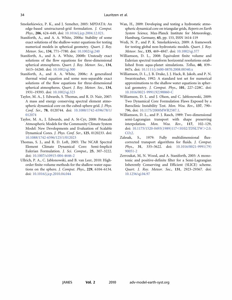
Smolarkiewicz, P. K., and J. Szmelter, 2005: MPDATA: An
edge-based unstructured-grid formulation. J. Comput.
Phys., 206, 624–649, doi: 10.1016/j.jcp.2004.12.021.
Staniforth, A., and A. A. White, 2008a: Stability of some
exact solutions of the shallow-water equations for testing
numerical models in spherical geometry. Quart. J. Roy.
Meteor. Soc., 134, 771–7780. doi: 10.1002/qj.240
Staniforth, A., and A. A. White, 2008b: Unsteady exact
solutions of the flow equations for three-dimensional
spherical atmospheres. Quart. J. Roy. Meteor. Soc., 134,
1615–16260. doi: 10.1002/qj.300
Staniforth, A., and A. A. White, 2008c: A generalized
thermal wind equation and some non-separable exact
solutions of the flow equations for three-dimensional
spherical atmospheres. Quart. J. Roy. Meteor. Soc., 134,
1931–19393. doi: 10.1002/qj.323
Taylor, M. A., J. Edwards, S. Thomas, and R. D. Nair, 2007:
A mass and energy conserving spectral element atmo-
spheric dynamical core on the cubed-sphere grid. J. Phys.
Conf. Ser., 78, 0120744. doi: 10.1088/1742-6596/78/1/
012074
Taylor, M. A., J. Edwards, and A. St-Cyr, 2008: Petascale
Atmospheric Models for the Community Climate System
Model: New Developments and Evaluation of Scalable
Dynamical Cores. J. Phys. Conf. Ser., 125, 0120233. doi:
10.1088/1742-6596/125/1/012023
Thomas, S. J., and R. D. Loft, 2005: The NCAR Spectral
Element Climate Dynamical Core: Semi-Implicit
Eulerian Formulation. J. Sci. Comput., 25, 307–3222.
doi: 10.1007/s10915-004-4646-2
Ullrich, P. A., C. Jablonowski, and B. van Leer, 2010: High-
order finite-volume methods for the shallow-water equa-
tions on the sphere. J. Comput. Phys., 229, 6104–6134.
doi: 10.1016/j.jcp.2010.04.044
Wan, H., 2009: Developing and testing a hydrostatic atmo-
spheric dynamical core on triangular grids, Reports on Earth
System Science, Max-Planck Institute for Meteorology,
Hamburg, Germany, 65, pp. 153, ISSN 1614-119
Wedi, N. P., and P. K. Smolarkiewicz, 2009: A framework
for testing global non-hydrostatic models. Quart. J. Roy.
Meteor. Soc., 135, 469–4847. doi: 10.1002/qj.377
Williamson, D. L., 2008: Equivalent finite volume and
Eulerian spectral transform horizontal resolutions estab-
lished from aqua-planet simulations. Tellus, 60, 839–
847x. doi: 10.1111/j.1600-0870.2008.00340.x
Williamson, D. L., J. B. Drake, J. J. Hack, R. Jakob, and P. N.
Swarztrauber, 1992: A standard test set for numerical
approximations to the shallow water equations in spher-
ical geometry. J. Comput. Phys., 101, 227–228C. doi:
10.1016/0021-9991(92)90060-C
Williamson, D. L. and J. Olson, and C. Jablonowski, 2009:
Two Dynamical Core Formulation Flaws Exposed by a
Baroclinic Instability Test. Mon. Wea. Rev., 137, 790–
796, doi: 10.1175/2008MWR2587.1.
Williamson, D. L., and P. J. Rasch, 1989: Two-dimensional
semi-Lagrangian transport with shape preserving
interpolation. Mon. Wea. Rev., 117, 102–129,
doi: 10.1175/1520-0493(1989)117,0102:TDSLTW.2.0.
CO;2.
Zalesak, S., 1979: Fully multidimensional flux-
corrected transport algorithms for fluids. J. Comput.
Phys., 31, 335–3622. doi: 10.1016/0021-9991(79)
90051-2
Zerroukat, M, N. Wood, and A. Staniforth, 2005: A mono-
tonic and positive-definite filter for a Semi-Lagrangian
Inherently Conserving and Efficient (SLICE) scheme.
Quart. J. Roy. Meteor. Soc., 131, 2923–29367. doi:
10.1256/qj.04.97
34 Lauritzen et al.
JAMES Vol. 2 2010 adv-model-earth-syst.org


![Baroclinic stationary waves in aquaplanet modelscentaur.reading.ac.uk/16701/2/16701_2011jas3573.1[1].pdf · 2020. 7. 4. · Baroclinic Stationary Waves in Aquaplanet Models GIUSEPPE](https://img.pdfslide.us/doc/110x75/61137b8b2d5ae1006a2d34ea/baroclinic-stationary-waves-in-aquaplanet-1pdf-2020-7-4-baroclinic-stationary.jpg)