Baroclinic Vortices in Rotating Stratified Shearing Flows: Cyclones,Anticyclones, and Zombie Vortices

by

Pedram Hassanzadeh

A dissertation submitted in partial satisfaction of the

requirements for the degree of

Doctor of Philosophy

in

Engineering – Mechanical Engineering

in the

Graduate Division

of the

University of California, Berkeley

Committee in charge:

Professor Philip S. Marcus, ChairProfessor Tarek I. ZohdiProfessor Edgar Knobloch

Spring 2013

Baroclinic Vortices in Rotating Stratified Shearing Flows: Cyclones,Anticyclones, and Zombie Vortices

Copyright 2013by

Pedram Hassanzadeh

1

Abstract

Baroclinic Vortices in Rotating Stratified Shearing Flows: Cyclones, Anticyclones, andZombie Vortices

by

Pedram Hassanzadeh

Doctor of Philosophy in Engineering – Mechanical Engineering

University of California, Berkeley

Professor Philip S. Marcus, Chair

Large coherent vortices are abundant in geophysical and astrophysical flows. They playsignificant roles in the Earth’s oceans and atmosphere, the atmosphere of gas giants, such asJupiter, and the protoplanetary disks around forming stars. These vortices are essentiallythree–dimensional (3D) and baroclinic, and their dynamics are strongly influenced by therotation and density stratification of their environments. This work focuses on improvingour understanding of the physics of 3D baroclinic vortices in rotating and continuouslystratified flows using 3D spectral simulations of the Boussinesq equations, as well as simplifiedmathematical models. The first chapter discusses the big picture and summarizes the resultsof this work.

In Chapter 2, we derive a relationship for the aspect ratio (i.e., vertical half–thicknessover horizontal length scale) of steady and slowly–evolving baroclinic vortices in rotatingstratified fluids. We show that the aspect ratio is a function of the Brunt-Vaisala frequencieswithin the vortex and outside the vortex, the Coriolis parameter, and the Rossby numberof the vortex. This equation is basically the gradient–wind equation integrated over thevortex, and is significantly different from the previously proposed scaling laws that find theaspect ratio to be only a function of the properties of the background flow, and indepen-dent of the dynamics of the vortex. Our relation is valid for cyclones and anticyclones ineither the cyclostrophic or geostrophic regimes; it works with vortices in Boussinesq fluidsor ideal gases, and non–uniform background density gradient. The relation for the aspectratio has many consequences for quasi–equilibrium vortices in rotating stratified flows. Forexample, cyclones must have interiors more stratified than the background flow (i.e., super–stratified), and weak anticyclones must have interiors less stratified than the background(i.e., sub–stratified). In addition, this equation is useful to infer the height and internalstratification of some astrophysical and geophysical vortices because direct measurements oftheir vertical structures are difficult. We verify our relation for the aspect ratio with numer-ical simulations for a wide variety of families of vortices, including: vortices that are initiallyin (dissipationless) equilibrium and then evolve due to an imposed weak viscous dissipation

2

or density radiation; anticyclones created by the geostrophic adjustment of a patch of lo-cally mixed density; cyclones created by fluid suction from a small localized region; vorticescreated from the remnants of the violent breakups of columnar vortices; and weakly non-axisymmetric vortices. The values of the aspect ratios of our numerically–computed vorticesvalidate our theoretically–derived relationship for aspect ratio, and generally they differ sig-nificantly from the values obtained from the much–cited conjecture that the aspect ratio ofquasi-geostrophic vortices is equal to the ratio of the Coriolis parameter to the Brunt-Vaisalafrequency of the background flow.

In Chapter 3, we show numerically and experimentally that localized suction in rotatingcontinuously stratified flows produces three–dimensional baroclinic cyclones. As expectedfrom Chapter 2, the interiors of these cyclones are super–stratified. Suction, modeled asa small spherical sink in the simulations, creates an anisotropic flow toward the sink withdirectional dependence changing with the ratio of the Coriolis parameter to the Brunt-Vaisalafrequency. Around the sink, this flow generates cyclonic vorticity and deflects isopycnals sothat the interior of the cyclone becomes super-stratified. The super–stratified region isvisualized in the companion experiments that we helped to design and analyze using thesynthetic schlieren technique. Once the suction stops, the cyclones decay due to viscousdissipation in the simulations and experiments. The numerical results show that the verticalvelocity of viscously decaying cyclones flows away from the cyclone’s midplane, while theradial velocity flows toward the cyclone’s center. This observation is explained based on thecyclo–geostrophic balance. This vertical velocity mixes the flow inside and outside of cycloneand reduces the super–stratification. We speculate that the predominance of anticyclonesin geophysical and astrophysical flows is due to the fact that anticyclones require sub–stratification, which occurs naturally by mixing, while cyclones require super–stratification.

In Chapter 4, we show that a previously unknown instability creates space–filling latticesof 3D turbulent baroclinic vortices in linearly–stable, rotating, stratified shear flows. Theinstability starts from a newly discovered family of easily–excited critical layers. This newfamily, named the baroclinic critical layer, has singular vertical velocities; the traditionalfamily of (barotropic) critical layer has singular stream–wise velocities and is hard to excite.In our simulations, the baroclinic critical layers in rotating stably–stratified linear shear areexcited by small–volume, small–amplitude vortices or waves. The excited baroclinic criticallayers then intensify by drawing energy from the background shear and roll–up into largecoherent 3D vortices that excite new critical layers and vortices. The vortices self–similarlyreplicate to create lattices of turbulent vortices. These vortices persist for all time and arecalled zombie vortices because they can occur in the dead zones of protoplanetary disks. Theself–replication of zombie vortices can de-stabilize the otherwise linearly and finite–amplitudestable Keplerian shear and lead to the formation of stars and planets.

i

Everything should be made as simple as possible, but not simplerA. Einstein

ii

Contents

Contents ii

1 Geophysical and Astrophysical Vortices 1

2 Universal Aspect Ratio of Baroclinic Vortices 72.1 Introduction . . . . . . . . . . . . . . . . . . . . . . . . . . . . . . . . . . . . 72.2 Aspect Ratio: Derivation . . . . . . . . . . . . . . . . . . . . . . . . . . . . . 82.3 Previously Proposed Scaling Laws . . . . . . . . . . . . . . . . . . . . . . . . 112.4 Gaussian Solution to the Dissipationless Boussinesq Equations . . . . . . . . 132.5 Numerical Simulation of the Boussinesq Equations . . . . . . . . . . . . . . . 142.6 Numerical Results for Vortex Aspect Ratios . . . . . . . . . . . . . . . . . . 152.7 Aspect Ratio: Numerical Simulations . . . . . . . . . . . . . . . . . . . . . . 182.8 Conclusion . . . . . . . . . . . . . . . . . . . . . . . . . . . . . . . . . . . . . 21

3 Baroclinic Cyclones Produced by Localized Suction 243.1 Introduction . . . . . . . . . . . . . . . . . . . . . . . . . . . . . . . . . . . . 243.2 Laboratory Experiment . . . . . . . . . . . . . . . . . . . . . . . . . . . . . . 263.3 Mathematical Formulation and Numerical Simulation . . . . . . . . . . . . . 283.4 Relative Effect of Rotation versus Stratification . . . . . . . . . . . . . . . . 313.5 Flow Field During Suction . . . . . . . . . . . . . . . . . . . . . . . . . . . . 343.6 Flow Field After Suction Stops . . . . . . . . . . . . . . . . . . . . . . . . . 403.7 Conclusion . . . . . . . . . . . . . . . . . . . . . . . . . . . . . . . . . . . . . 47

4 Self–Replicating 3D Vortices in Stably–Stratified Rotating Shear 494.1 Introduction . . . . . . . . . . . . . . . . . . . . . . . . . . . . . . . . . . . . 494.2 Critical Layers . . . . . . . . . . . . . . . . . . . . . . . . . . . . . . . . . . . 514.3 Single Vortex Perturbation . . . . . . . . . . . . . . . . . . . . . . . . . . . . 544.4 Conclusion . . . . . . . . . . . . . . . . . . . . . . . . . . . . . . . . . . . . . 56

A Suction Rate Function qo(x) 58

Bibliography 60

iii

Acknowledgments

It was the best of times, it was the age of wisdom, it was the epoch of belief, it was the seasonof Light, it was the spring of hope, I had everything before me; these words well describe myfive years in UC Berkeley as a Ph.D. student. I owe this great time to a group of amazingpeople and here is a chance to thank some of them.

First and foremost, I would like to thank my Ph.D. advisor Philip Marcus. Phil’s passion,devotion, depth and breadth of knowledge, energy, integrity, and kindness the most perfectPh.D. advisor I could have dreamed of. He patiently taught me fluid dynamics, math,computation, and geophysical fluid dynamics; he also showed me how to approach a newproblem, how to simplify it, and how not to oversimplify it. I am grateful to Phil forthoughtfully mentoring me through the first two years of my Ph.D., and then giving memore freedom and flexibly while providing invaluable input, guidance, and criticism. Not farinto my Ph.D., I started to think of Phil as not only my advisor but also as a friend (thesmarter, more experienced kind of friend everybody looks for), and I would like to thank himfor all of his advice and support. Thank you Phil for this wonderful and rewarding journey.

I am very grateful to my labmate Chung-Hsiang Jiang for what he has patiently taughtme, for his help with computation, and for his great advice about research, coursework,career, etc. I would like to deeply thank another labmate, Suyang Pei, for our wonderfulcollaboration over the past five years; I learned so much from Suyang, and he has beenalways extremely generous in sharing his ideas and results, and very patient with explainingthem to me. Working with Chung-Hsiang and Suyang made my Ph.D. way more fruitful andenjoyable. I would like to express my gratitude toward Oriane Aubert, Patrice Le Gal, andMichael Le Bars in IRPHE for our productive and stimulating collaboration. Furthermore,I am very grateful to Patrice for teaching me a lot about waves, instabilities, vortices, andexperiments; for his kind support in various occasions; and for showing me how a scientificcollaboration can be fun as well. I would like to thank Oriane for our numerous Skypeconversations about vortices and rotating stratified flows. I appreciate Michael’s support,and his feedback and contribution to this work.

I would like to thank Omer Savas for teaching me fluid mechanics, for his advice andsupport throughout the years, and for chairing my qualifying exam. Much appreciationgoes to the members of my qualifying exam and dissertation committees: Tarek Zohdi, PerPersson, David Steigmann, and Edgar Knobloch. In particular, I am grateful to Edgar forhis comments on my dissertation, for his support, and for his wonderful course on dynamicalsystems, which showed me how much math I do not know. I truly enjoyed and benefited fromthe well-taught courses that I took in UC Berkeley. In addition to Phil, Omer, Edgar, David,and Per, I would like to thank Panos Papadopoulos, John Neu, James Sethian, AlexandreChorin, Grigory Barenblatt, and Van Carey.

I spent the summer of 2012 as a GFD Fellow at the Woods Hole Oceanographic Institutionwhere I worked with Charlie Doering and Greg Chini. They insightfully guided me throughthe well-designed and exciting project, and I sincerely appreciate their devotion and support.I would like to thank all the fellows and participants of the GFD program, in particular

iv

George Veronis, for this wonderful experience. I would like to thank Jon Wilkening for acareful review of this work, which was turned into a master’s thesis in mathematics. InWoods Hole, I greatly enjoyed and benefited from the lectures by Jeff Weiss on vortices andcoherent structures. He clarified many subtle key points for me.

I would like to thank the current and former members of our lab: Joe Barranco, SushilShetty, Xylar Asay–Davis, Meng Wang, Caleb Levy, Mani Mahdinia, Sahuck Oh, and OmidSolari. In particular, I am grateful to Joe for developing the parallel spectral code whichbecame the basis of my code, to Sushil for helpful suggestions and encouragement at thebeginning of my Ph.D., and to Caleb for his help with running and post-processing someof the simulations. I would like to thank Caleb and Kenneth Lee for carefully proofreadingparts of this dissertation. I appreciate scholarships form the Natural Sciences and Engi-neering Research Council of Canada, the Woods Hole Oceanographic Institution, and theJonathan Laitone Memorial Scholarship Fund. I would also like to thank the staff in BrewedAwakening, especially P. J. and Eric, for their good coffee and friendly chitchat.

I am very grateful to George Raithby, my master’s thesis advisor in the University ofWaterloo, for accepting me as his student, for teaching me computation and heat transfer,and above all, for helping me to mature and transform from an undergraduate student to agraduate student and researcher. George (along with my friend Amir Baserinia) also helpedme to adapt to the culture and environment, and he gently forced me to improve my English(which I did by watching each episode of Seinfeld 10 times). I would also like to thankGordon Stubley and Metin Renksizbulut for the well–taught courses and for their support.

I would like to thank Vahid Esfahanian who introduced me to the amazing world of fluiddynamics and computation in my sophomore year. He then hired me in his lab and providedme a great opportunity to do research and acquire valuable skills. I have been using what Ilearned from Vahid almost every day in grad school. Furthermore, I am grateful to FarschadTorabi and Ahmad Javaheri (famil) for being great teachers, supporters, and friends. As anundergrad, I learned so much from courses offered by Mehrdad Raisee and Mehdi Ashjaee. Iwould also like to thank Mehrdad for his support, and for encouraging me to study abroad.

I have been blessed with great friends in my life, and they have generously shared theirthoughts, time, knowledge, and happiness with me. Some of these friends have had a deepimpact on my life and have made me a much better and happier person. Thank you SaraToutiaei, Ashkan Borna, Arman Hajati, Arash Tajik, Azad Zade, Saba Pasha, Kenny Lee,Sobhan Seyfaddini, Farzaneh Shahrokhi, Donna Artusy, Alireza Lahijanian, Heather Kittel,Nader Norouzi, Mehdi Dargahi, Sahar Tabesh, Amin Arbabian, Azadeh Bozorgzadeh, Ben-jamin Jarrahi, Nasim Alem, Jay Keist, Arash Raisee, Farzad Houshmand, Meysam Rezaee,Mohsen Shahini, Laleh Davis, Mehrzad Tartibi, Caroline Uhler, Debanjan Mukherjee, Ba-hador Jafarpur, Sunny Mistry, Giorgio de Vera . . .

Above all, I am indebted to my great family, my parents Safa and Hossein and mysister Pegah, for their endless and selfless love, encouragement, and support. Words cannotdescribe my love for them, and my gratitude for what they have done for me.

1

Chapter 1

Geophysical and AstrophysicalVortices

Large coherent vortices are abundant in geophysical and astrophysical flows. These persistentvortices, which are tens to millions of kilometers in diameter, strongly interact with theirenvironment. For example, vortices of the Agulhas Current (Figure 1.1) and Mediterraneaneddies, called Meddies, (Figure 1.2) carry warm water into the Atlantic ocean and transporta huge amount of salinity, nutrients, and chemicals for large distances [Armi et al., 1988,Klein and Lapeyre, 2009]. Tropical cyclones [Rossby, 1949] and polar vortices [McIntyre,1995] are examples of vortices in the Earth’s atmosphere; the latter play an important rolein the stratospheric dynamics and have contributed to the ozone depletion [McIntyre, 1989,Waugh and Polvani, 2010]. Studying the physics of geophysical vortices and their impacton the oceanic and atmospheric circulations, climate, and the ecosystem is an active area ofresearch. However, the difficulties of in–situ measurements and well–resolved simulations oflarge–scale flows pose a big challenge to these studies [Siegel et al., 2001, Khouider et al.,2013, Ghil et al., 2008].

Atmospheres of the gas giants are also filled with large long–lived vortices. Examplesare Jupiter’s Great Red Spot [Hooke, 1665] and Oval BA [Go et al., 2006] (Figure 1.3),Saturn’s polar vortices [Godfrey, 1988, Sanchez-Lavega et al., 2006] and Neptune’s GreatDark Spot [Smith et al., 1989]. These vortices cause significant mixing and transport of heatacross these planets and their disappearance might lead to a global climate change [Marcus,2004]. Although some of these vortices, such as the Great Red Spot, have been extensivelystudied, many questions about their color and color–change [Wong et al., 2011, Marcus et al.,2013a], longevity [Ingersoll and Cuong, 1981, Vasavada and Showman, 2005, Sommeria et al.,1988], vertical and horizontal structures [de Pater et al., 2010, Fletcher et al., 2010, Morales-Juberıas and Dowling, 2013], and interaction with the zonal flows [Salyk et al., 2006, Shettyet al., 2007, Marcus, 1988] are still not answered.

Vortices exist even beyond our solar system. It has been speculated [Abramowicz et al.,1992] that coherent vortices play an important role in the formation of stars [McKee andOstriker, 2007] and planets [Lissauer, 1993] in the protoplanetary disks. This is because

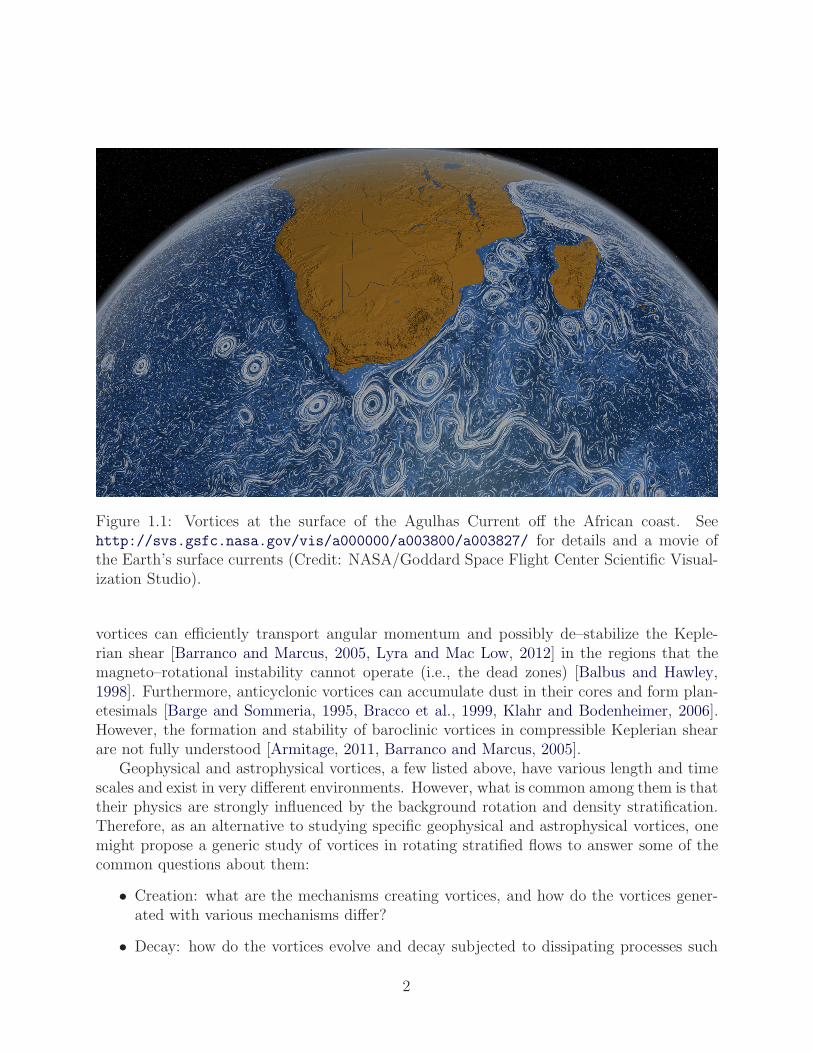
Figure 1.1: Vortices at the surface of the Agulhas Current off the African coast. Seehttp://svs.gsfc.nasa.gov/vis/a000000/a003800/a003827/ for details and a movie ofthe Earth’s surface currents (Credit: NASA/Goddard Space Flight Center Scientific Visual-ization Studio).

vortices can efficiently transport angular momentum and possibly de–stabilize the Keple-rian shear [Barranco and Marcus, 2005, Lyra and Mac Low, 2012] in the regions that themagneto–rotational instability cannot operate (i.e., the dead zones) [Balbus and Hawley,1998]. Furthermore, anticyclonic vortices can accumulate dust in their cores and form plan-etesimals [Barge and Sommeria, 1995, Bracco et al., 1999, Klahr and Bodenheimer, 2006].However, the formation and stability of baroclinic vortices in compressible Keplerian shearare not fully understood [Armitage, 2011, Barranco and Marcus, 2005].

Geophysical and astrophysical vortices, a few listed above, have various length and timescales and exist in very different environments. However, what is common among them is thattheir physics are strongly influenced by the background rotation and density stratification.Therefore, as an alternative to studying specific geophysical and astrophysical vortices, onemight propose a generic study of vortices in rotating stratified flows to answer some of thecommon questions about them:

• Creation: what are the mechanisms creating vortices, and how do the vortices gener-ated with various mechanisms differ?

• Decay: how do the vortices evolve and decay subjected to dissipating processes such

2

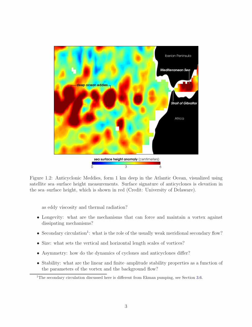
Figure 1.2: Anticyclonic Meddies, form 1 km deep in the Atlantic Ocean, visualized usingsatellite sea–surface height measurements. Surface signature of anticyclones is elevation inthe sea–surface height, which is shown in red (Credit: University of Delaware).

as eddy viscosity and thermal radiation?

• Longevity: what are the mechanisms that can force and maintain a vortex againstdissipating mechanisms?

• Secondary circulation1: what is the role of the usually weak meridional secondary flow?

• Size: what sets the vertical and horizontal length scales of vortices?

• Asymmetry: how do the dynamics of cyclones and anticyclones differ?

• Stability: what are the linear and finite–amplitude stability properties as a function ofthe parameters of the vortex and the background flow?

1The secondary circulation discussed here is different from Ekman pumping, see Section 3.6.

3

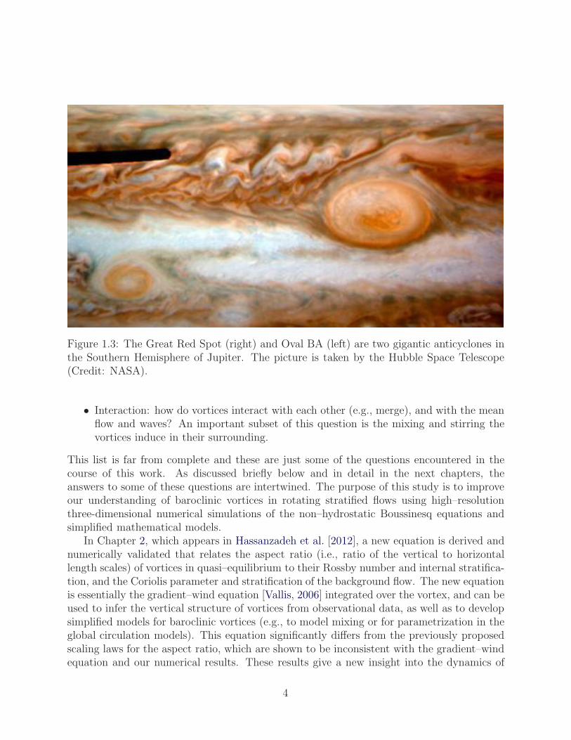
Figure 1.3: The Great Red Spot (right) and Oval BA (left) are two gigantic anticyclones inthe Southern Hemisphere of Jupiter. The picture is taken by the Hubble Space Telescope(Credit: NASA).

• Interaction: how do vortices interact with each other (e.g., merge), and with the meanflow and waves? An important subset of this question is the mixing and stirring thevortices induce in their surrounding.

This list is far from complete and these are just some of the questions encountered in thecourse of this work. As discussed briefly below and in detail in the next chapters, theanswers to some of these questions are intertwined. The purpose of this study is to improveour understanding of baroclinic vortices in rotating stratified flows using high–resolutionthree-dimensional numerical simulations of the non–hydrostatic Boussinesq equations andsimplified mathematical models.

In Chapter 2, which appears in Hassanzadeh et al. [2012], a new equation is derived andnumerically validated that relates the aspect ratio (i.e., ratio of the vertical to horizontallength scales) of vortices in quasi–equilibrium to their Rossby number and internal stratifica-tion, and the Coriolis parameter and stratification of the background flow. The new equationis essentially the gradient–wind equation [Vallis, 2006] integrated over the vortex, and can beused to infer the vertical structure of vortices from observational data, as well as to developsimplified models for baroclinic vortices (e.g., to model mixing or for parametrization in theglobal circulation models). This equation significantly differs from the previously proposedscaling laws for the aspect ratio, which are shown to be inconsistent with the gradient–windequation and our numerical results. These results give a new insight into the dynamics of

4

the baroclinic vortices and in particular the role of the secondary circulation. The simula-tions show that the interior stratifications of a vortex evolves in time and space because of ameridional secondary circulation induced by weak dissipating processes. The weak secondarycirculation is also found to affect the time evolution of the velocity field of the vortex andchange the Rossby number.

In ongoing work not presented in this dissertation, numerical results show that the decayof dissipating vortices, in particular in the presence of zonal shear, can be significantlyslowed down by the secondary circulation because of its capability to efficiently convertthe kinetic energy to potential energy and vice versa (preliminary results are presentedin Marcus and Hassanzadeh [2011] and Hassanzadeh and Marcus [2012]). These resultsmight explain the unexpected longevity2 of some of the oceanic [Armi et al., 1989] andplanetary vortices [Ingersoll, 1990] with no need of a strong forcing mechanism. Note thatmost numerical studies in the past have used hydrostatic or two–dimensional models resultingin the secondary circulation being either absent or not accurately represented.

Chapter 3, which appears in Hassanzadeh et al. [2013], discusses one of the mechanismsto produce baroclinic vortices in nature and in laboratory: localized suction. Numericalsimulations and laboratory experiments show that a baroclinic cyclone with an interior morestratified than the background flow (i.e., super–stratified) is produced as a result of suction.The fact that the cyclones have super–stratified interiors, as opposed to anticyclones whichhave less stratified interiors, can be a major contributor to the cyclone–anticyclone asym-metry in rotating stratified turbulence. The role of the secondary circulation in mixing theinside and outside of the cyclone and reducing the super–stratification once the suction stopsis also studied.

Chapter 4, which appears in Marcus et al. [2013b], presents a new family of criticallayers for rotating stably–stratified shear that has singularity in vertical velocities3. High–resolution three–dimensional simulations show that baroclinic critical layers are easily exitedby a single small–volume vortex, form stripes of strong vertical vorticity, and subsequentlyroll up and produce new vortices, which in turn excite new layers. The vortices self–replicateand populate the entire computational domain. This instability is expected to be ubiquitousin the dead zones of the protoplanetary disks. Such purely hydrodynamic instability inthe dead zones has been long searched for in simulations and experiments without success[Balbus and Hawley, 1998, Ji et al., 2006, Paoletti et al., 2012]. We believe that the barocliniccritical layers and their instability have not been observed previously because of one or moreof the following in the past studies: focusing on constant–density fluids in most experimentsand some simulations; small apparatuses and parameter–regime in some experiments; lackof resolution, using hydrostatic models, unphysical initial conditions, and performing two–dimensional simulations in many of the computational studies.

2For example, the Great Red Spot has survived for over 300 years despite having a radiative time scaleof ≈ 10 years [Marcus, 1993].

3See Boulanger et al. [2007] for an analytical and experimental analysis of a similar but not quite thesame family of critical layers.

5

Apart from improving our answers to some of the questions asked before (e.g., aspect ratioand vertical structure, creation, secondary circulation, etc.), this work demonstrates thatimportant aspects of the physics of geophysical and astrophysical flows may be missed in two–dimensional or hydrostatic simulations, or in studies that ignore the vertical stratification;hence “everything should be made as simple as possible, but not simpler”.

6

7

Chapter 2

Universal Aspect Ratio of BaroclinicVortices

2.1 Introduction

Compact three–dimensional baroclinic vortices are abundant in geo- and astrophysical flows.Examples in planetary atmospheres include the rows of cyclones and anticyclones near Sat-urn’s Ribbon [Sayanagi et al., 2010] and near 41◦S on Jupiter [Humphreys and Marcus, 2007],and Jupiter’s anticyclonic Great Red Spot [Marcus, 1993]. In the Atlantic ocean, meddiespersist for years [Armi et al., 1988, McWilliams, 1985], and numerical simulations of thedisks around protostars produce compact anticyclones [Barranco and Marcus, 2005]. Thephysics that create, control, and decay these vortices are highly diverse, and the aspect ra-tios α ≡ H/L of these vortices range from flat “pancakes” to nearly round (where H is thevertical half-height and L is the horizontal length scale of the vortex). However, we shallshow that the aspect ratios of the vortices all obey a universal relationship.

Our relation for α differs from previously published ones, including the often-used α =

f/N , where f is the Coriolis parameter, N ≡√

−gρ∂ρ∂z

is the Brunt-Vaisala frequency, g is

the acceleration of gravity, z is the vertical coordinate, ρ is the density for Boussinesq flowsand potential density for compressible flows; and a bar over a quantity indicates that it isthe value of the unperturbed (i.e., with no vortices) background flow. We shall show thatα = f/N is not only incorrect by factors of 10 or more in some cases, but also that it ismisleading; it suggests that α depends only on the background flow and not on the propertiesof the vortex, so that all vortices embedded in the same flow (e.g., in the Atlantic or in theJovian atmosphere) have the same α. We shall show that this is not true. Knowledge of the

With minor modifications, Chapter 1 is reprinted with permission from:P. Hassanzadeh, P. S. Marcus, and P. Le Gal, The Universal Aspect Ratio of Vortices in Rotating StratifiedFlows: Theory and Simulation, Journal of Fluid Mechanics, (706), 2012.

correct relation for α is important. For example, there has been debate over whether thecolor change, from white to red, of Jupiter’s anticyclone Oval BA, was due to a change inits H [de Pater et al., 2010]. Measurements of the half-heights H of planetary vortices aredifficult, but H could be accurately inferred if the correct relation for α were known. Wevalidate our relation for α with 3D numerical simulations of the Boussinesq equations. Acompanion paper by [Aubert et al., 2012] validates it with laboratory experiments and withobservations of Atlantic ocean meddies and Jovian vortices.

2.2 Aspect Ratio: Derivation

We assume that the rotation axis and gravity are parallel and anti-parallel to the verticalz axis, respectively. We also assume that the vortices are in approximate cyclo-geostrophicbalance horizontally and hydrostatic balance vertically (referred to hereafter as CG-H bal-ance). Necessary approximations for CG-H balance are that the vertical vz and radial vrvelocities are negligible compared to the azimuthal one vθ (where the origin of the cylindricalcoordinate system is at the vortex center), that dissipation is negligible, and that the flowis approximately steady in time. With these approximations, the radial r and azimuthal θcomponents of Euler’s equation in a rotating frame are

∂p

∂r= ρvθ

(f +

vθr

)(2.1)

∂p

∂z= −ρg, (2.2)

where p is the pressure. We have assumed that the vortex is axisymmetric, but we showlater numerically in Section 2.7 that this approximation can be relaxed. Following theconvention, we ignored the centrifugal term ρf 2r/4 r in equation (2.1) by assuming that thecentrifugal buoyancy is much smaller than the gravitational buoyancy, i.e. that the rotationalFroude number f 2d/(4g) � 1, where d is the characteristic distance of the vortex from therotation axis [see e.g. Barcilon and Pedlosky, 1967]. The θ-component of Euler’s equation,continuity equation, and the equation governing the dissipationless transport of (potential)density are all satisfied by a steady, axisymmetric flow with vr = vz = 0. As a consequence,equations (2.1) and (2.2) are the only equations that need to be satisfied for both Boussinesqand compressible flows. Thus, our relation for α will also be valid for both of these flows.Far from the vortex, where v = 0, p = p, and ρ = ρ, (2.1) and (2.2) reduce to

∂p

∂r= 0 (2.3)

∂p

∂z= −ρg (2.4)

8

showing that p and ρ are only functions of z. Subtracting equations (2.3) and (2.4) from(2.1) and (2.2):

∂p

∂r= ρvθ

(f +

vθr

)(2.5)

∂p

∂z= −ρg (2.6)

where p ≡ p − p and ρ ≡ ρ − ρ are respectively the pressure and density anomalies. Thecenter of a vortex (r = z = 0) is defined as the location on the z-axis where p has itsextremum, so equation (2.6) shows that at the vortex center (denoted by a c subscript)ρc = 0 or ρc = ρ(0) ≡ ρo. At the vortex boundary and outside the vortex, where vθ and ρare negligible, equations (2.5) and (2.6) show that p � 0.

We define the pressure anomaly’s characteristic horizontal length scale (i.e. radius) as

L ≡√∣∣∣∣ 4pc

(∇2⊥p)c

∣∣∣∣, (2.7)

where the subscript ⊥ means horizontal component. Integrating (2.5) from the vortex centerto its side boundary at (r, z) = (L, 0) approximately yields

− pcL

= ρoVθ

(f +

VθRv

)(2.8)

where in the course of integration, ρ has been replaced with ρo, which is exact for Boussinesqflows, and an approximation for fully compressible flows. Here Vθ is the characteristic peakazimuthal velocity, and Rv is the approximate radius where the velocity has that peak. Theanalytical and numerically simulated vortices discussed below, meddies, and the laboratoryvortices examined by [Aubert et al., 2012] all have Rv ≈ L, but hollow vortices with quiescentinteriors have Rv �= L. For example, the Great Red Spot has Rv � 3L [Shetty and Marcus,2010]. Similarly, integrating (2.6) from the vortex center to its top boundary at (r, z) = (0, H)approximately gives

pcH

= gρ(r = 0, z = H), (2.9)

where H is the pressure anomaly’s characteristic vertical length scale (i.e. half-height),

H ≡√∣∣∣∣ 2pc

(∂2p/∂z2)c

∣∣∣∣. (2.10)

Equations (2.8) and (2.9) can be combined to eliminate pc:

ρoVθ(f + Vθ/Rv)

H= −gρ(r = 0, z = H)

L. (2.11)

9

Notice that this equation is basically the thermal wind equation, with the cyclostrophic termincluded (i.e. the gradient-wind equation [Vallis, 2006]), integrated over the vortex. Usingthe first term of a Taylor series, we approximate ρ(r = 0, z = H) on the right-hand side of(2.11) with

ρ(r = 0, z = H) = ρc +H(∂ρ/∂z)c

= H [(∂ρ/∂z)c − (∂ρ/∂z)c]

= ρoH(N2 −N2c )/g (2.12)

where ρ ≡ ρ − ρ and ρc = 0 have been used. Note that in general, N(z) is a function ofz; however, the only way in which N(z) is used in this derivation (or anywhere else in thispaper) is at z = 0 for evaluating (∂ρ/∂z)c. Therefore, rather than using the cumbersomenotation Nc, we simply use N .

Using (2.12) in equation (2.11) gives our relation for α:

α2 ≡(H

L

)2

=Ro [1 + (L/Rv)Ro]

N2c − N2

f 2 (2.13)

where the Rossby number defined as Ro ≡ Vθ/(fL) can be well approximated as

Ro = ωc/(2f), (2.14)

ωc being the vertical component of vorticity at the vortex center. Defining the Burger numberas

Bu ≡(NH

fL

)2

, (2.15)

equation (2.13) may be as well rewritten as[(Nc

N

)2

− 1

]Bu = Ro

[1 +

L

RvRo

](2.16)

Equation (2.13) shows that α depends on two properties of the vortex: Ro and thedifference between the Brunt-Vaisala frequencies inside the vortex (i.e. N2

c ) and outsidethe vortex (i.e. N2). Note that to derive relation (2.13), no assumption has been madeon the compressibility of the flow, Rossby number smallness, dependence of N on z, or themagnitude of Nc/N . Therefore, equation (2.13) is applicable to Boussinesq, anelastic [Vallis,2006], and fully compressible flows, cyclones (i.e., Ro > 0) and anticyclones (i.e., Ro < 0),and geostrophic and cyclostrophic flows. In the cyclostrophic limit (i.e., |Ro| 1) withNc = 0 and Rv = L,

Ro (1 +Ro) → Ro2, (2.17)

10

hence equation (2.13) becomes Vθ = HN , agreeing with the findings of [Billant and Chomaz,2001] and others. Equation (2.13) is easily modified for use with discrete layers of fluid ratherthan a continuous stratification, and in that case agrees with the work of [Nof, 1981] and[Carton, 2001].

Equation (2.13) has several consequences for equilibrium vortices. For example, becausethe right-hand side of (2.13) must be positive, cyclones must have N2

c ≥ N2. Anotherconsequence is that anticyclones with −Ro < Rv/L, must have N2

c ≤ N2, and anticycloneswith −Ro > Rv/L, have N

2c ≥ N2. In addition, equation (2.13) is useful for astrophysical

and geophysical observations of vortices in which some of the vortex properties are difficultto measure. For example, Nc is difficult to measure in some ocean vortices [Aubert et al.,2012], and H is difficult to determine in some satellite observations of atmospheric vortices[de Pater et al., 2010], but their values can be inferred from equation (2.13).

Note that Nc is a measure of the mixing within the vortex; if the density is not mixedwith respect to the background flow, then Nc → N (and the vortex is a tall, barotropicTaylor column); if the density is well-mixed within the vortex so the (potential) density isuniform inside the vortex, then Nc → 0 (as in the experiments of [Aubert et al., 2012]); ifN2

c > N2 (as required by cyclones), then the vortex is more stratified than the backgroundflow.

2.3 Previously Proposed Scaling Laws

Other relations for α that differ from our equation (2.13) have been published previously,and the most frequently cited one is

α ≡ H

L=

f

N. (2.18)

This relationship is inferred from Charney’s equation for the quasi-geostrophic (QG) poten-tial vorticity [equation (8) in Charney, 1971] that was derived for flows with |Ro| � 1 andNc/N � 1. Separately re-scaling the vertical and horizontal coordinates of the potentialvorticity equation, and then assuming that the vortices are isotropic in the re-scaled (butnot physical) coordinates, one obtains the alternative scaling α = f/N . Numerical simula-tions of the QG equation for some initial conditions have produced turbulent vortices withH/L ≈ f/N [c.f., McWilliams et al., 1999, Dritschel et al., 1999, Reinaud et al., 2003], eventhough significant anisotropy in the re-scaled coordinates was observed in similar simulations[McWilliams et al., 1994]. The constraints under which the QG equation is derived are veryrestrictive; for example, none of meddies or laboratory vortices studied by [Aubert et al.,2012] meet these requirements because Nc/N is far from unity. Therefore, it is not surpris-ing that none of these vortices, including the laboratory vortices, agree with α ≈ f/N , butinstead have α in accord with relation (2.13) [Aubert et al., 2012].

The constraints under which our equation (2.13) for α is derived are far less restrictivethan those used in deriving Charney’s QG equation (and we never need to assume isotropy).

11

In particular, one of several constraints needed for deriving Charney’s QG equation is thescaling required for the potential temperature (his equation (3)), which written in terms ofthe potential density is

ρ

ρ= −f

g

∂ψ

∂z, (2.19)

where ψ is the stream function of horizontal velocity. This constraint alone (which is ef-fectively the thermal wind equation) implies our relationship (2.13) for α. To see this, inequation (2.19) replace

ψ with VθL, (2.20)

∂

∂zwith

1

H, (2.21)

Vθ with RofL, (2.22)

ρ

ρwith

H

ρ

[(∂ρ

∂z

)c

− ∂ρ

∂z

]=H

g

(N2 −N2

c

). (2.23)

With these replacements, equation (2.19) immediately gives(H

L

)2

= Rof 2

N2c − N2

, (2.24)

which is the small Ro limit of equation (2.13).Gill [1981] also proposed a relationship for α that differs from ours. He based his relation

for α on a model 2D zonal flow (that is, not an axisymmetric vortex, but rather a 2D vortex)and found that α was proportional to

Ro f/N.

To determine α, Gill derived separate solutions for the flow inside and outside his 2D modelvortex, which he assumed was dissipationless and in geostrophic and hydrostatic balance.Despite the fact that Gill’s published relation for α, obtained from the outside solution,differs from ours, we can show that his solution for the flow inside his 2D vortex satisfies ourscaling relation for α: Gill’s solution for the zonal velocity (which is in the y direction) is

v = −(f/a)x (2.25)

(his equation (5.14) in dimensional form). His density anomaly is

ρ = ρo (N2/g) z (2.26)

(i.e. within the 2D vortex, ρ = ρo). The equation for v gives ωz = −(f/a), and therefore

Ro ≡ ωc

2f= − 1

2a(2.27)

12

Substituting v and ρ into the equations for geostrophic and hydrostatic balance, gives

∂p

∂x= −ρo f

2

ax (2.28)

and

∂p

∂z= −ρo N2 z (2.29)

respectively. Using the definitions of H and L from Section 2.2 along with Ro = −1/(2a),we obtain

α2 = −Ro f2

N2, (2.30)

which is our relation (2.13) in the limit of small Ro, L = Rv, and Nc = 0 (which are theconstraints under which Gill’s solution is obtained). Gill’s scaling for α is derived from theflow outside the vortex, which he derived by requiring that both the tangential velocity anddensity are continuous at the interface between the inside and outside solutions. In general,this over–constrains the dissipationless flow (which only requires pressure and normal veloc-ity to be continuous – see for example the vortex solution in Aubert et al. [2012] in which thepressure and normal component of the velocity are continuous at the interface, but not thedensity or tangential velocity.) The extra constraints force the solution outside Gill’s vortexto have additional (unphysical) length scales, resulting in Gill’s relation for α differing fromours. Aubert et al. [2012] show that Gill’s relationship for α does not fit their laboratoryexperiments, meddies, or Jovian vortices. We examine the accuracy of both Charney’s andGill’s relationships in Section 2.7.

2.4 Gaussian Solution to the Dissipationless

Boussinesq Equations

It is possible to find closed–form solutions to the steady, axisymmetric, dissipationless Boussi-nesq equations (e.g. [Aubert et al., 2012]). One solution that we shall use to generate initialconditions for our initial–value codes is the Gaussian vortex with

p = pc exp[−(z/H)2 − (r/L)2] (2.31)

vr = 0 (2.32)

vz = 0 (2.33)

where pc, H , and L are arbitrary constants. Then, ρ is found from ∂p/∂z using equation (2.6),and vθ is found from ∂p/∂r using equation (2.5) with ρ replaced by ρo. This Gaussian vortexexactly obeys our relationship (2.13) for α when the Rossby number is defined as before as

13

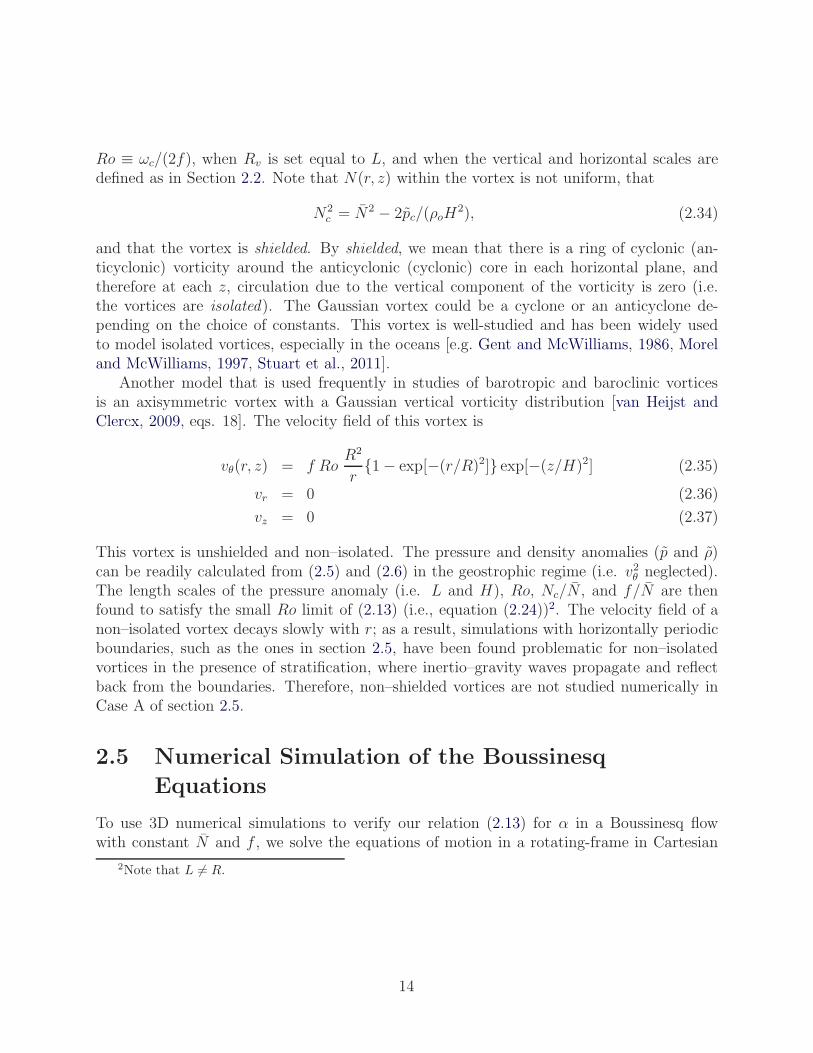
Ro ≡ ωc/(2f), when Rv is set equal to L, and when the vertical and horizontal scales aredefined as in Section 2.2. Note that N(r, z) within the vortex is not uniform, that

N2c = N2 − 2pc/(ρoH

2), (2.34)

and that the vortex is shielded. By shielded, we mean that there is a ring of cyclonic (an-ticyclonic) vorticity around the anticyclonic (cyclonic) core in each horizontal plane, andtherefore at each z, circulation due to the vertical component of the vorticity is zero (i.e.the vortices are isolated). The Gaussian vortex could be a cyclone or an anticyclone de-pending on the choice of constants. This vortex is well-studied and has been widely usedto model isolated vortices, especially in the oceans [e.g. Gent and McWilliams, 1986, Moreland McWilliams, 1997, Stuart et al., 2011].

Another model that is used frequently in studies of barotropic and baroclinic vorticesis an axisymmetric vortex with a Gaussian vertical vorticity distribution [van Heijst andClercx, 2009, eqs. 18]. The velocity field of this vortex is

vθ(r, z) = f RoR2

r{1− exp[−(r/R)2]} exp[−(z/H)2] (2.35)

vr = 0 (2.36)

vz = 0 (2.37)

This vortex is unshielded and non–isolated. The pressure and density anomalies (p and ρ)can be readily calculated from (2.5) and (2.6) in the geostrophic regime (i.e. v2θ neglected).The length scales of the pressure anomaly (i.e. L and H), Ro, Nc/N , and f/N are thenfound to satisfy the small Ro limit of (2.13) (i.e., equation (2.24))2. The velocity field of anon–isolated vortex decays slowly with r; as a result, simulations with horizontally periodicboundaries, such as the ones in section 2.5, have been found problematic for non–isolatedvortices in the presence of stratification, where inertio–gravity waves propagate and reflectback from the boundaries. Therefore, non–shielded vortices are not studied numerically inCase A of section 2.5.

2.5 Numerical Simulation of the Boussinesq

Equations

To use 3D numerical simulations to verify our relation (2.13) for α in a Boussinesq flowwith constant N and f , we solve the equations of motion in a rotating-frame in Cartesian

2Note that L �= R.

14

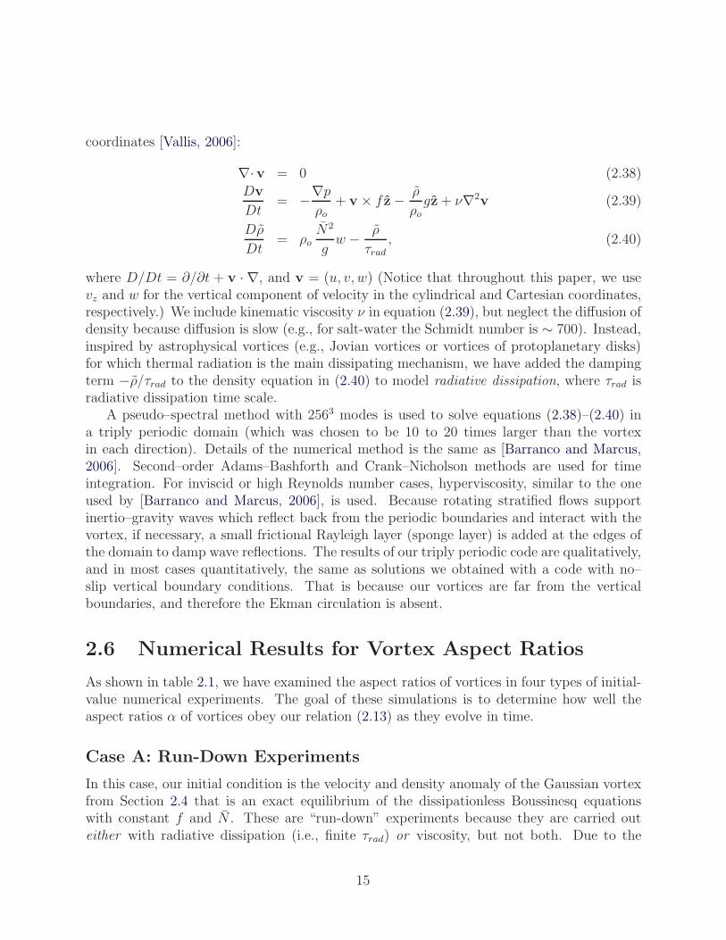
coordinates [Vallis, 2006]:

∇·v = 0 (2.38)

Dv

Dt= −∇p

ρo+ v × f z− ρ

ρogz+ ν∇2v (2.39)

Dρ

Dt= ρo

N2

gw − ρ

τrad, (2.40)

where D/Dt = ∂/∂t + v · ∇, and v = (u, v, w) (Notice that throughout this paper, we usevz and w for the vertical component of velocity in the cylindrical and Cartesian coordinates,respectively.) We include kinematic viscosity ν in equation (2.39), but neglect the diffusion ofdensity because diffusion is slow (e.g., for salt-water the Schmidt number is ∼ 700). Instead,inspired by astrophysical vortices (e.g., Jovian vortices or vortices of protoplanetary disks)for which thermal radiation is the main dissipating mechanism, we have added the dampingterm −ρ/τrad to the density equation in (2.40) to model radiative dissipation, where τrad isradiative dissipation time scale.

A pseudo–spectral method with 2563 modes is used to solve equations (2.38)–(2.40) ina triply periodic domain (which was chosen to be 10 to 20 times larger than the vortexin each direction). Details of the numerical method is the same as [Barranco and Marcus,2006]. Second–order Adams–Bashforth and Crank–Nicholson methods are used for timeintegration. For inviscid or high Reynolds number cases, hyperviscosity, similar to the oneused by [Barranco and Marcus, 2006], is used. Because rotating stratified flows supportinertio–gravity waves which reflect back from the periodic boundaries and interact with thevortex, if necessary, a small frictional Rayleigh layer (sponge layer) is added at the edges ofthe domain to damp wave reflections. The results of our triply periodic code are qualitatively,and in most cases quantitatively, the same as solutions we obtained with a code with no–slip vertical boundary conditions. That is because our vortices are far from the verticalboundaries, and therefore the Ekman circulation is absent.

2.6 Numerical Results for Vortex Aspect Ratios

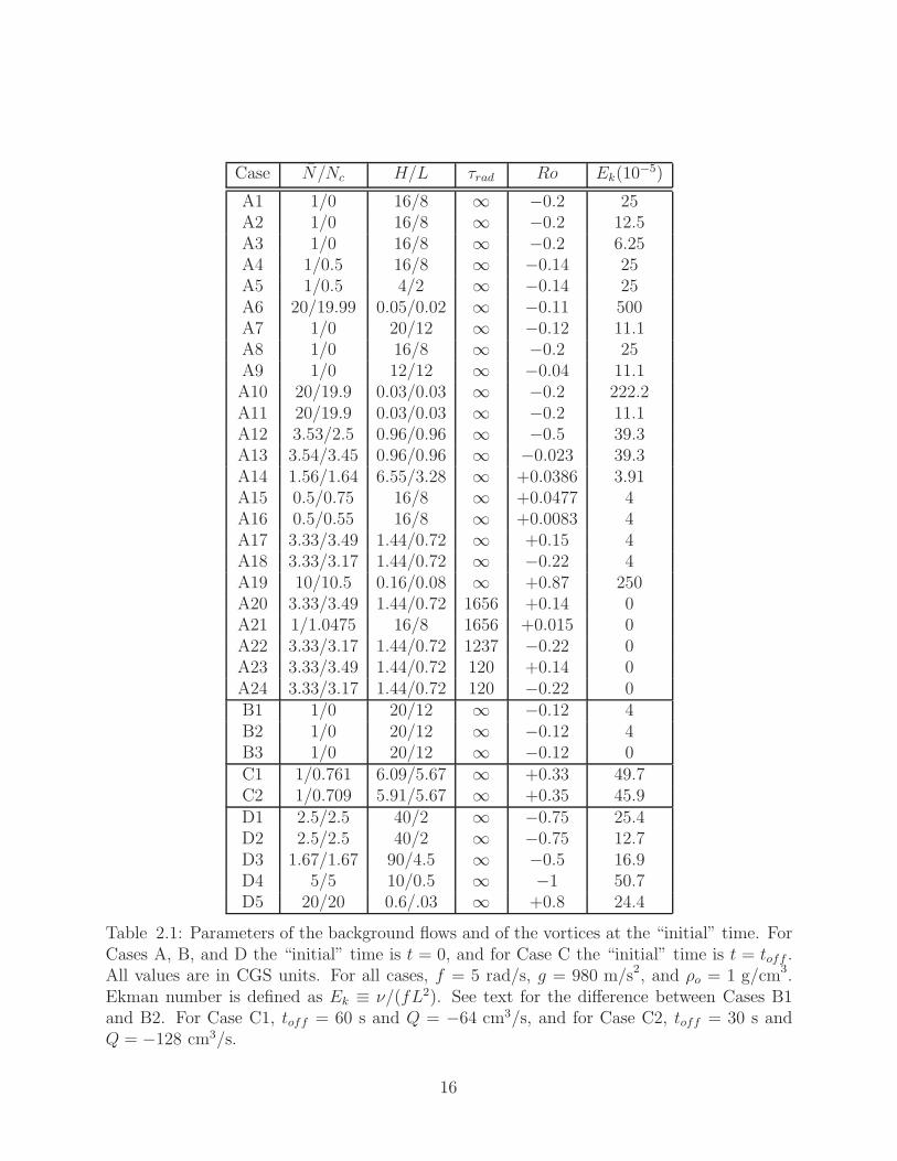
As shown in table 2.1, we have examined the aspect ratios of vortices in four types of initial-value numerical experiments. The goal of these simulations is to determine how well theaspect ratios α of vortices obey our relation (2.13) as they evolve in time.

Case A: Run-Down Experiments

In this case, our initial condition is the velocity and density anomaly of the Gaussian vortexfrom Section 2.4 that is an exact equilibrium of the dissipationless Boussinesq equationswith constant f and N . These are “run-down” experiments because they are carried outeither with radiative dissipation (i.e., finite τrad) or viscosity, but not both. Due to the

15

Case N/Nc H/L τrad Ro Ek(10−5)

A1 1/0 16/8 ∞ −0.2 25A2 1/0 16/8 ∞ −0.2 12.5A3 1/0 16/8 ∞ −0.2 6.25A4 1/0.5 16/8 ∞ −0.14 25A5 1/0.5 4/2 ∞ −0.14 25A6 20/19.99 0.05/0.02 ∞ −0.11 500A7 1/0 20/12 ∞ −0.12 11.1A8 1/0 16/8 ∞ −0.2 25A9 1/0 12/12 ∞ −0.04 11.1A10 20/19.9 0.03/0.03 ∞ −0.2 222.2A11 20/19.9 0.03/0.03 ∞ −0.2 11.1A12 3.53/2.5 0.96/0.96 ∞ −0.5 39.3A13 3.54/3.45 0.96/0.96 ∞ −0.023 39.3A14 1.56/1.64 6.55/3.28 ∞ +0.0386 3.91A15 0.5/0.75 16/8 ∞ +0.0477 4A16 0.5/0.55 16/8 ∞ +0.0083 4A17 3.33/3.49 1.44/0.72 ∞ +0.15 4A18 3.33/3.17 1.44/0.72 ∞ −0.22 4A19 10/10.5 0.16/0.08 ∞ +0.87 250A20 3.33/3.49 1.44/0.72 1656 +0.14 0A21 1/1.0475 16/8 1656 +0.015 0A22 3.33/3.17 1.44/0.72 1237 −0.22 0A23 3.33/3.49 1.44/0.72 120 +0.14 0A24 3.33/3.17 1.44/0.72 120 −0.22 0B1 1/0 20/12 ∞ −0.12 4B2 1/0 20/12 ∞ −0.12 4B3 1/0 20/12 ∞ −0.12 0C1 1/0.761 6.09/5.67 ∞ +0.33 49.7C2 1/0.709 5.91/5.67 ∞ +0.35 45.9D1 2.5/2.5 40/2 ∞ −0.75 25.4D2 2.5/2.5 40/2 ∞ −0.75 12.7D3 1.67/1.67 90/4.5 ∞ −0.5 16.9D4 5/5 10/0.5 ∞ −1 50.7D5 20/20 0.6/.03 ∞ +0.8 24.4

Table 2.1: Parameters of the background flows and of the vortices at the “initial” time. ForCases A, B, and D the “initial” time is t = 0, and for Case C the “initial” time is t = toff .All values are in CGS units. For all cases, f = 5 rad/s, g = 980 m/s2, and ρo = 1 g/cm3.Ekman number is defined as Ek ≡ ν/(fL2). See text for the difference between Cases B1and B2. For Case C1, toff = 60 s and Q = −64 cm3/s, and for Case C2, toff = 30 s andQ = −128 cm3/s.

16

weak dissipation, the vortices slowly evolve (decay) and do not remain Gaussian. Also, asa result of the dissipation (and decay), a weak secondary flow is induced (i.e. non-zero vrand vz). The secondary flows and their roles are further discussed in Chapter 3, Marcus andHassanzadeh [2011], and Hassanzadeh and Marcus [2012].

Case B: Vortices Generated by Geostrophic Adjustment

This case is motivated by vortices produced from the geostrophic adjustment of a locallymixed patch of density, e.g. generated from diapycnal mixing [see e.g. McWilliams, 1988,Stuart et al., 2011]. Our flow is initialized with v = 0 and ρ �= 0. For Cases B1 and B3 theinitial ρ is that of the Gaussian vortex discussed in Section 2.4. But here, the initial flow isfar from equilibrium because v ≡ 0. In Case B2, the initial ρ is Gaussian in r, but has atop-hat function in z (for this case, the initial H is defined as the half-height of the top-hatfunction). It is observed in the numerical simulations that geostrophic adjustment quicklyproduces shielded vortices.

Case C: Cyclones Produced by Suction

Injection of fluid into a rotating flow generates anticyclones [Aubert et al., 2012], whilesuction produces cyclones. We simulate suction by modifying the continuity equation (2.38)as

∇ · v = Q(x, t) (2.41)

where Q is a specified suction rate function and x = (x, y, z). The flow is initialized withv = ρ = 0. Suction starts at t = 0 over a spherical region with radius of 6 cm and is turnedoff at time toff . A shielded cyclone is produced and strengthened during the suction process.As mentioned at the end of Section 2.2, for Ro > 0, relation (2.13) requires the flow tobe superstratified (i.e. Nc > N). Our numerical simulations show that the initial suctioncreates super–stratification. Cases C1 and C2 have different suction rates and toff , but thesame total sucked volume of fluid, and it is observed that the produced cyclones are similar.The dynamics of cyclones produced by localized suction are explored in details in Chapter 3.

Case D: Vortices Produced from the Breakup of Tall Barotropic

Vortices

The violent breakup of tall barotropic (z-independent) vortices in rotating stratified flowscan produce stable compact vortices [see e.g. Smyth and McWilliams, 1998]. In Case D, ourflows are initialized with an unstable 2D columnar vortex with

vθ = Ro f r exp(−(r/L)2) (2.42)

and ρ = 0 (for this case, the initial H is the vertical height of the computational domain).Note that the initial columnar vortex is shielded. Noise is added to the initial velocity field

17

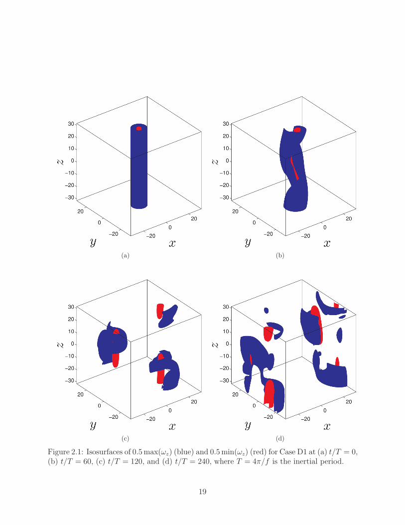
to hasten instabilities. The vortex breaks up and then the remnants equilibrate to one ormore compact shielded vortices (Figure 2.1). In each case, only the vortex with the largest|Ro| is analyzed in Section 2.7.

2.7 Aspect Ratio: Numerical Simulations

In all cases, vortices reach quasi-equilibrium and then slowly decay due to viscous or radiativedissipation except for Case B3 which is dissipationless and evolves only due to geostrophicadjustment. As a result, Ro decreases, and the mixing of density in the vortex interiorchanges (i.e., Nc changes). Therefore, it is not surprising that the aspect ratio α also changesin time. Quasi-equilibrium is reached in Case A almost immediately. In Case B, vorticesquickly form and come to quasi-equilibrium after geostrophic adjustment. Quasi-equilibriumis achieved following the geostrophic and hydrostatic adjustments after toff in Case C, and(much longer) after the initial instabilities in Case D.

For each case, we use the results of the numerical simulations to calculate

Ro(t) ≡ ωc(t)

2f(2.43)

and

Nc(t) ≡√N2 − g

ρo

(∂ρ(x, t)

∂z

)c

(2.44)

We compute L(t) and H(t) from the numerical solutions using their definitions given inSection 2.2. Calculating L based on ∇2

⊥ rather than just r-derivatives is useful for non-axisymmetric vortices. For example, due to a small non-axisymmetric perturbation addedto the initial condition of Case A8, the vortex went unstable and produced a tripole [vanHeijst and Kloosterziel, 1989]. Cases C1 and C2 also produced non-axisymmetric vortices.We define the numerical aspect ratio as

αNUM(t) ≡ H(t)

L(t). (2.45)

We define the theoretical aspect ratio αTHR from equation (2.13) using Ro(t) and Nc(t)extracted from the numerical results and the (constant) values of f and N .

Figure 2.2 shows how well αTHR agrees with αNUM. The inset in Figure 2.2 shows thatthe relative difference between the two values, calculated as

|1− (αNUM/αTHR)2|,

is smaller than 0.07. For each case, the maximum difference occurs at early times or duringinstabilities.

18

(a) (b)

(c) (d)

Figure 2.1: Isosurfaces of 0.5max(ωz) (blue) and 0.5min(ωz) (red) for Case D1 at (a) t/T = 0,(b) t/T = 60, (c) t/T = 120, and (d) t/T = 240, where T = 4π/f is the inertial period.

19

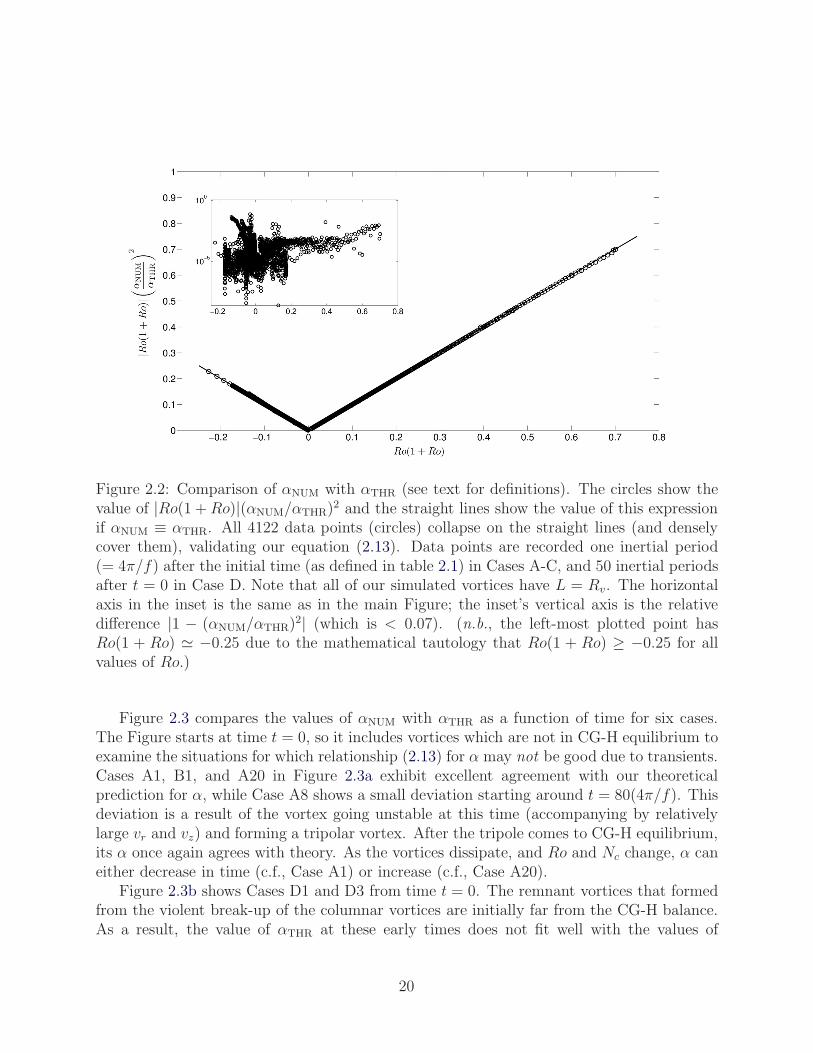
Figure 2.2: Comparison of αNUM with αTHR (see text for definitions). The circles show thevalue of |Ro(1 +Ro)|(αNUM/αTHR)

2 and the straight lines show the value of this expressionif αNUM ≡ αTHR. All 4122 data points (circles) collapse on the straight lines (and denselycover them), validating our equation (2.13). Data points are recorded one inertial period(= 4π/f) after the initial time (as defined in table 2.1) in Cases A-C, and 50 inertial periodsafter t = 0 in Case D. Note that all of our simulated vortices have L = Rv. The horizontalaxis in the inset is the same as in the main Figure; the inset’s vertical axis is the relativedifference |1 − (αNUM/αTHR)

2| (which is < 0.07). (n.b., the left-most plotted point hasRo(1 + Ro) � −0.25 due to the mathematical tautology that Ro(1 + Ro) ≥ −0.25 for allvalues of Ro.)

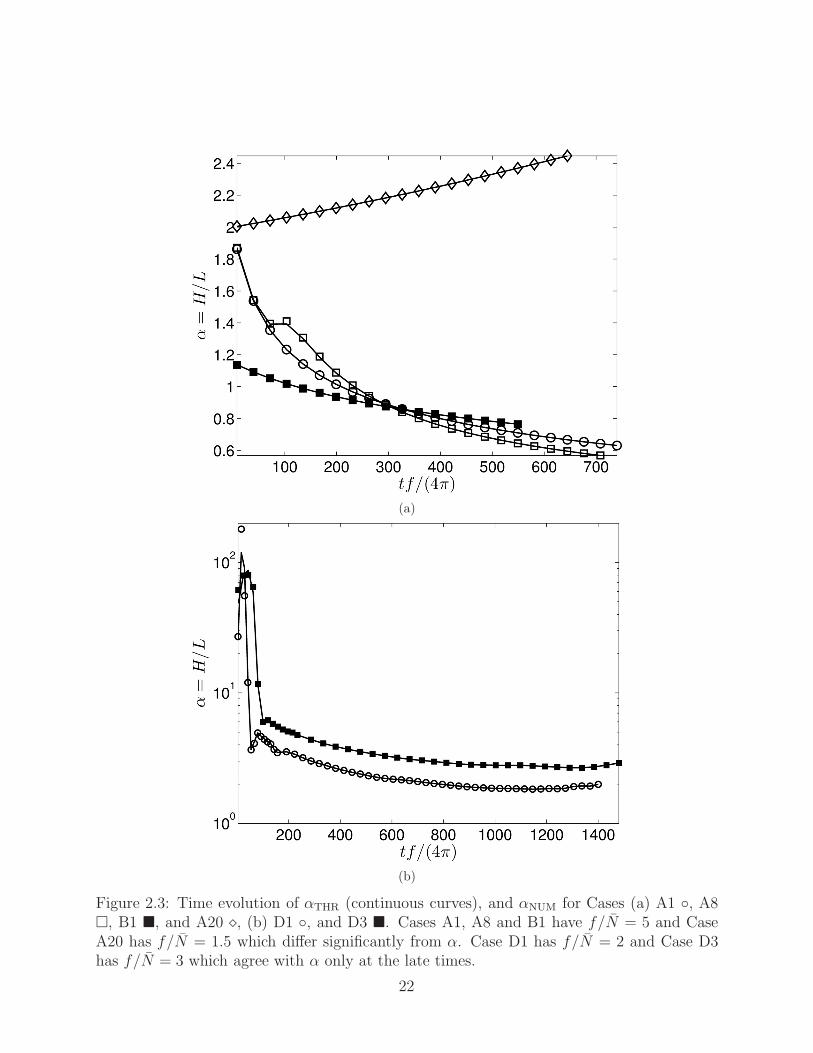
Figure 2.3 compares the values of αNUM with αTHR as a function of time for six cases.The Figure starts at time t = 0, so it includes vortices which are not in CG-H equilibrium toexamine the situations for which relationship (2.13) for α may not be good due to transients.Cases A1, B1, and A20 in Figure 2.3a exhibit excellent agreement with our theoreticalprediction for α, while Case A8 shows a small deviation starting around t = 80(4π/f). Thisdeviation is a result of the vortex going unstable at this time (accompanying by relativelylarge vr and vz) and forming a tripolar vortex. After the tripole comes to CG-H equilibrium,its α once again agrees with theory. As the vortices dissipate, and Ro and Nc change, α caneither decrease in time (c.f., Case A1) or increase (c.f., Case A20).

Figure 2.3b shows Cases D1 and D3 from time t = 0. The remnant vortices that formedfrom the violent break-up of the columnar vortices are initially far from the CG-H balance.As a result, the value of αTHR at these early times does not fit well with the values of

20

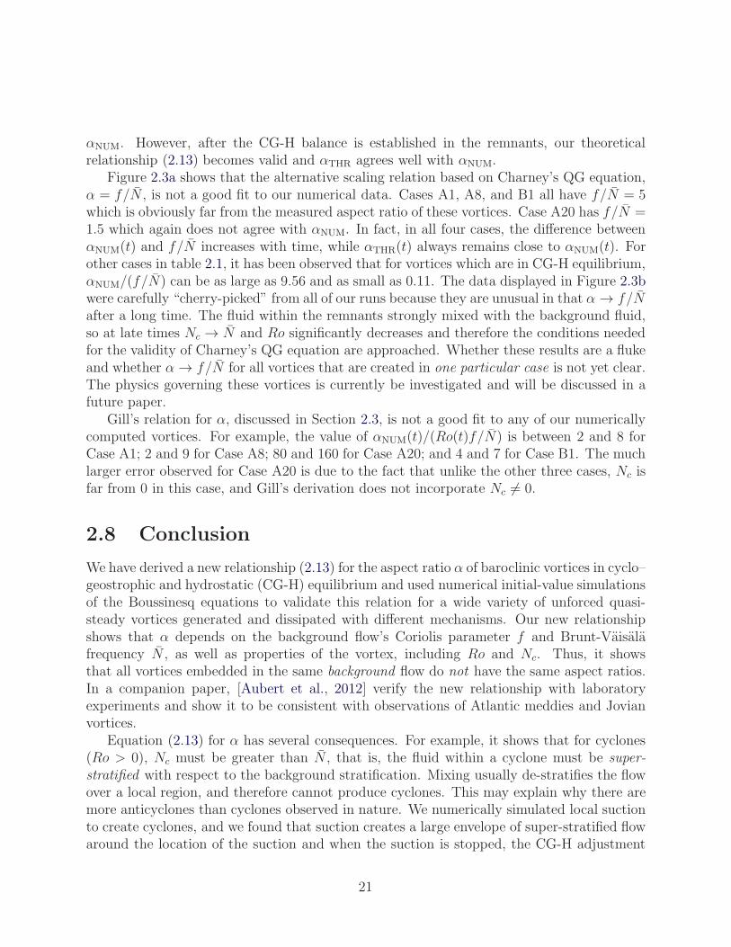
αNUM. However, after the CG-H balance is established in the remnants, our theoreticalrelationship (2.13) becomes valid and αTHR agrees well with αNUM.

Figure 2.3a shows that the alternative scaling relation based on Charney’s QG equation,α = f/N , is not a good fit to our numerical data. Cases A1, A8, and B1 all have f/N = 5which is obviously far from the measured aspect ratio of these vortices. Case A20 has f/N =1.5 which again does not agree with αNUM. In fact, in all four cases, the difference betweenαNUM(t) and f/N increases with time, while αTHR(t) always remains close to αNUM(t). Forother cases in table 2.1, it has been observed that for vortices which are in CG-H equilibrium,αNUM/(f/N) can be as large as 9.56 and as small as 0.11. The data displayed in Figure 2.3bwere carefully “cherry-picked” from all of our runs because they are unusual in that α → f/Nafter a long time. The fluid within the remnants strongly mixed with the background fluid,so at late times Nc → N and Ro significantly decreases and therefore the conditions neededfor the validity of Charney’s QG equation are approached. Whether these results are a flukeand whether α→ f/N for all vortices that are created in one particular case is not yet clear.The physics governing these vortices is currently be investigated and will be discussed in afuture paper.

Gill’s relation for α, discussed in Section 2.3, is not a good fit to any of our numericallycomputed vortices. For example, the value of αNUM(t)/(Ro(t)f/N) is between 2 and 8 forCase A1; 2 and 9 for Case A8; 80 and 160 for Case A20; and 4 and 7 for Case B1. The muchlarger error observed for Case A20 is due to the fact that unlike the other three cases, Nc isfar from 0 in this case, and Gill’s derivation does not incorporate Nc �= 0.

2.8 Conclusion

We have derived a new relationship (2.13) for the aspect ratio α of baroclinic vortices in cyclo–geostrophic and hydrostatic (CG-H) equilibrium and used numerical initial-value simulationsof the Boussinesq equations to validate this relation for a wide variety of unforced quasi-steady vortices generated and dissipated with different mechanisms. Our new relationshipshows that α depends on the background flow’s Coriolis parameter f and Brunt-Vaisalafrequency N , as well as properties of the vortex, including Ro and Nc. Thus, it showsthat all vortices embedded in the same background flow do not have the same aspect ratios.In a companion paper, [Aubert et al., 2012] verify the new relationship with laboratoryexperiments and show it to be consistent with observations of Atlantic meddies and Jovianvortices.

Equation (2.13) for α has several consequences. For example, it shows that for cyclones(Ro > 0), Nc must be greater than N , that is, the fluid within a cyclone must be super-stratified with respect to the background stratification. Mixing usually de-stratifies the flowover a local region, and therefore cannot produce cyclones. This may explain why there aremore anticyclones than cyclones observed in nature. We numerically simulated local suctionto create cyclones, and we found that suction creates a large envelope of super-stratified flowaround the location of the suction and when the suction is stopped, the CG-H adjustment

21

(a)

(b)

Figure 2.3: Time evolution of αTHR (continuous curves), and αNUM for Cases (a) A1 ◦, A8�, B1 �, and A20 �, (b) D1 ◦, and D3 �. Cases A1, A8 and B1 have f/N = 5 and CaseA20 has f/N = 1.5 which differ significantly from α. Case D1 has f/N = 2 and Case D3has f/N = 3 which agree with α only at the late times.

22

makes cyclones. Details of these simulations and results of an ongoing laboratory experimentwill be presented in subsequent publications.

It is widely quoted that vortices obey the quasi-geostrophic scaling law α = f/N (i.e.Burger number Bu = 1). This is inconsistent with our relationship which written in termsof Bu is

Bu =Ro(1 +Ro)

(Nc/N)2 − 1(2.46)

We found that, with the exception of one family of vortices, the quasi-geostrophic scalinglaw was not obeyed by the vortices studied here (and by Aubert et al. [2012]), and could beincorrect by more than a factor of 10. Another relationship proposed by Gill [1981] was alsofound to produce very poor predictions of aspect ratio.

We found that α can either increase or decrease as the vortex decays, and our relation-ship (2.13) shows that the dependence of α on Nc is specially sensitive when Nc is at theorder of N , as it is for meddies and Jovian vortices [Aubert et al., 2012]. Our simulationsshowed that Nc was determined by the secondary circulations within a vortex and that thosecirculations are controlled by the dissipation. In a future paper we shall report on the detailsof how dissipation determines the secondary flows and the temporal evolution of Nc, bothof which are important in planetary atmospheres, oceanic vortices, accretion disk flows, andplanet formation [Barranco and Marcus, 2005].

23

24

Chapter 3

Baroclinic Cyclones Produced byLocalized Suction

3.1 Introduction

Vortices that swirl in the same (opposite) direction as (of) the background rotation are calledcyclones (anticyclones). Both cyclones and anticyclones exist in the oceans [Olson, 1991], butlarge long–lived vortices are predominantly anticyclonic [see e.g. McWilliams, 1985, Sangraet al., 2009, Perret et al., 2011]. Cyclones and anticyclones also exist in the atmosphere ofJupiter [Vasavada and Showman, 2005] and Saturn [Sayanagi et al., 2010], but large long–lived vortices are mostly anticyclonic [Mac Low and Ingersoll, 1986, Cho and Polvani, 1996b].For example, Jupiter’s Great Red Spot and White Ovals [Marcus, 1993], Red Oval [Go et al.,2006], and Neptune’s Great Dark Spot [Smith et al., 1989] are all anticyclones.

The cyclone–anticyclone asymmetry is also observed in experimental and numerical stud-ies and has received considerable attention in recent years. In rotating constant–densityflows, cyclones and anticyclones form 2D Taylor columns and their dynamics differ due tothe ageostrophic effects. Most numerical and laboratory studies found cyclonic predominancein strongly rotating constant–density flows [see Moisy et al., 2010, and references therein].On the other hand, the cyclone–anticyclone asymmetry in rotating stratified flows, wherevortices are essentially 3D [Hassanzadeh et al., 2012, Aubert et al., 2012], is still contro-versial. Most numerical simulations of shallow–water or primitive equations [Polvani et al.,1994, Cho and Polvani, 1996a, Koszalka et al., 2009] and laboratory experiments [Lindenet al., 1995, Perret et al., 2006] have shown the predominance of coherent anticyclones in

With minor modifications, Chapter 3 appears in:P. Hassanzadeh, O. Aubert, P. S. Marcus, M. Le Bars, and P. Le Gal, Three–Dimensional Cyclones Producedby Localized Suction in Rotating Stratified Flows: a Numerical and Experimental Study, to be submitted tothe Journal of Fluid Mechanics, 2013.

rotating stratified flow. (Note that the quasi–geostrophic equations are degenerate with re-spect to the cyclone–anticyclone asymmetry, see e.g. Pedlosky [1990].) In contrast to thesestudies, some laboratory experiments [Praud et al., 2006] and numerical simulations withboundary dynamics [Hakim et al., 2002, Roullet and Klein, 2010] have reported cyclonicpredominance.

The dominance of anticyclones in most simulations, experiments, and observations canbe due to one or more of the following: (1) the creation mechanisms favor anticyclonesover cyclones [McWilliams, 1985, Perret et al., 2011], (2) anticyclones are more stable thancyclones [Stegner and Dritschel, 2000, Graves et al., 2006], (3) anticyclones are easier toobserve [Marcus, 2004], (4) anticyclones have greater longevity compared to cyclones, and(5) cyclones exist in a smaller parameter regime than anticyclones. All of these possibilities,in particular the last two, need further investigation.

Cyclones have low–pressure centers so that in a horizontal plane, the radially inwardpressure force balances the radially outward Coriolis and centrifugal forces [Kundu andCohen, 2010]. To support the low–pressure core in the vertical, a baroclinic cyclone must havean interior more stratified than the surrounding flow, so that the buoyancy force balances thepressure force [Hassanzadeh et al., 2012, Aubert et al., 2012, also see Section 3.6]. Conversely,baroclinic anticyclones in geostrophic balance have high–pressure cores and interiors lessstratified than their environments. Therefore, the dynamics of cyclones and anticyclones instrongly rotating stratified flows differ not only because of the nonlinear effects, but alsobecause of their dissimilar internal stratification. The consequences of the latter for thestability and longevity of the vortices has not been fully explored.

A region that is more stratified than the background flow (e.g., inside a cyclone) is calledsuper–stratified hereafter. For a process to produce cyclones in near cyclo–geostrophic andhydrostatic balances, a super–stratified region has to be created. It has been suggested byHassanzadeh et al. [2012] and Aubert et al. [2012] that the super–stratification requirementmay be a key factor in the sparsity of cyclones, because mixing, which is ubiquitous in naturebecause of turbulence, tends to de–stratify the flow and produces regions of less stratification,and therefore favor anticyclones [McWilliams, 1985, 1988].

Localized suction (injection) is one of the standard methods used in laboratory exper-iments for producing barotropic cyclones (anticyclones) in rotating flows with constant–density [van Heijst and Clercx, 2009]. In rotating stratified flows, local injection of a constantdensity fluid has been used to produce 3D baroclinic anticyclones [Griffiths and Linden, 1981,Hedstrom and Armi, 1988, Bush and Woods, 1999, Aubert et al., 2012]. However, suctionhas not been used previously as a method of creating local super–stratification, and with theexception of Linden et al. [1995] and Cenedese and Linden [1999], has not been used to pro-duce cyclones in rotating stratified laboratory flows. In analytic and numerical studies usingthe linearized Boussinesq [McDonald, 1992], shallow–water [Davey and Killworth, 1989, Aikiand Yamagata, 2000, 2004], or quasi–geostrophic [Hines, 1997] equations, localized sourcesand sinks have been used to model buoyancy–driven circulation in the deep ocean and tomodel the generation of oceanic vortices.

In this paper we show that 3D baroclinic cyclones can be produced by localized suction

25

in a rotating, continuously stratified flow in both laboratory experiments and numericalsimulations. The purpose of this paper is to obtain a better understanding of how localizedsuction produces cyclonic vorticity and super–stratification. Such physical understanding iskey in designing experimental studies of cyclones, of the cyclone–anticyclone asymmetry, andalso in the investigation of natural processes that are modeled as localized sinks. Additionally,we investigate the dynamics of viscously decaying cyclones and the evolution of their super–stratified interior and meridional velocities (i.e., secondary circulation). The remainder ofthis section discusses why suction and injection are distinct phenomena and not the time–reverse of each other. In Section 3.2 we present the experimental setup, and in Section 3.3we rederive the Boussinesq equations to account for localized suction. Section 3.3 also brieflyreviews the numerical method used to solve these equations. Section 3.4 shows how rotationand stratification affect the symmetries of the flow. Sections 3.5 and 3.6 discuss the detailsof the flow field during suction and after the suction stops, respectively. Section 3.7 presentsour conclusion and plans for future work.

Suction versus Injection

We remind the reader that the suction/injection of viscous fluids from an orifice is nottime-reversible, and suction is therefore not the time–reverse of injection. Viscosity playsan important role in injection, particularly at the tip of the orifice where it forms a vortexsheet around a jet–like flow. On the other hand, suction has a more global effect: the fluidmoves toward the orifice from all directions, regardless of the orientation of the orifice [alsosee Linden et al., 1995]. As a result, a candle can be easily put out by blowing air, butnot (easily) by sucking air. Another manifestation of the suction–injection asymmetry isthe reverse sprinkler, i.e. a lawn sprinkler submerged in a pool of water sucking the waterin. A question raised by Ernest Mach and popularized by Richard Feynman in his memoirSurely You’re Joking, Mr. Feynman!, a reverse sprinkler in fact does not rotate becauseof the absence of jets that produce torque in regular sprinklers to overcome the frictionof the bearings [see Jenkins, 2004, for further discussion and historical accounts]. Thisunderstanding of suction will be exploited in Section 3.3 to derive the governing equationsmodified for localized suction.

3.2 Laboratory Experiment

A rotating tank partially filled with linearly stratified salt–water is used in the laboratoryexperiments (Figure 3.1). The apparatus is the same one used in Aubert et al. [2012] toproduce anticyclones by local injection. The square tank is 50× 50× 70 cm (all units in thispapers are in cgs). The Oster double–bucket method is used to produce a 30 cm deep layerof linearly stratified fluid around the midplane with density profile ρ(z) = ρo[1 − N2(z −15)/g], where N is the Brunt–Vaisala frequency and is constant in each experiment, g isthe acceleration of gravity, ρo is the density of pure water, and z is the vertical coordinate

26

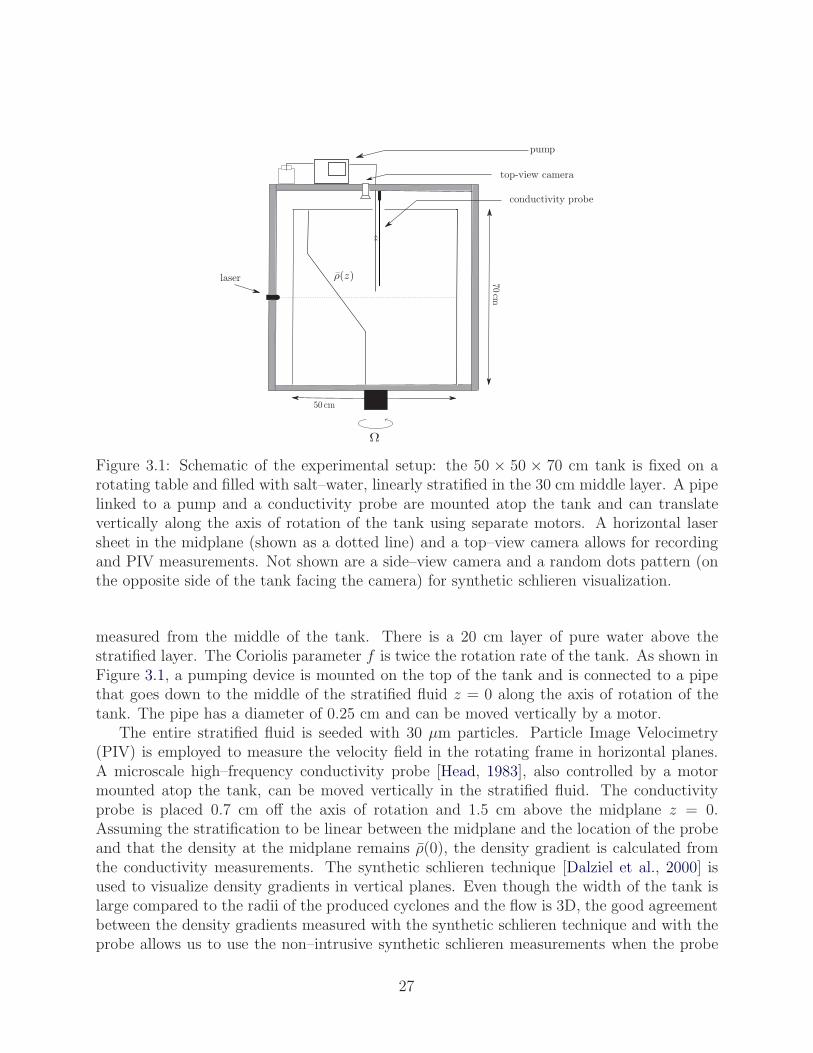
Figure 3.1: Schematic of the experimental setup: the 50 × 50 × 70 cm tank is fixed on arotating table and filled with salt–water, linearly stratified in the 30 cm middle layer. A pipelinked to a pump and a conductivity probe are mounted atop the tank and can translatevertically along the axis of rotation of the tank using separate motors. A horizontal lasersheet in the midplane (shown as a dotted line) and a top–view camera allows for recordingand PIV measurements. Not shown are a side–view camera and a random dots pattern (onthe opposite side of the tank facing the camera) for synthetic schlieren visualization.

measured from the middle of the tank. There is a 20 cm layer of pure water above thestratified layer. The Coriolis parameter f is twice the rotation rate of the tank. As shown inFigure 3.1, a pumping device is mounted on the top of the tank and is connected to a pipethat goes down to the middle of the stratified fluid z = 0 along the axis of rotation of thetank. The pipe has a diameter of 0.25 cm and can be moved vertically by a motor.

The entire stratified fluid is seeded with 30 μm particles. Particle Image Velocimetry(PIV) is employed to measure the velocity field in the rotating frame in horizontal planes.A microscale high–frequency conductivity probe [Head, 1983], also controlled by a motormounted atop the tank, can be moved vertically in the stratified fluid. The conductivityprobe is placed 0.7 cm off the axis of rotation and 1.5 cm above the midplane z = 0.Assuming the stratification to be linear between the midplane and the location of the probeand that the density at the midplane remains ρ(0), the density gradient is calculated fromthe conductivity measurements. The synthetic schlieren technique [Dalziel et al., 2000] isused to visualize density gradients in vertical planes. Even though the width of the tank islarge compared to the radii of the produced cyclones and the flow is 3D, the good agreementbetween the density gradients measured with the synthetic schlieren technique and with theprobe allows us to use the non–intrusive synthetic schlieren measurements when the probe

27

cannot be used because it disturbs the vortex.Once the stationary tank is filled with the linear stratification, the tank is rotated at a

fixed rate and the fluid is spun up to achieve near solid–body rotation (note that exact solid–body rotation cannot be achieved in the presence of diffusion, see e.g. von Zeipel [1924] andGreenspan [1990, pp. 12]). At this time, marked as t = 0, the pipe is moved down verticallyalong the center line of the tank to the midplane of the stratified fluid (i.e., z = 0). Fluidis then sucked out of the tank at a given volumetric rate Qo [cm3/s] for ts seconds. Aftersuction stops, the pipe is slowly removed from the fluid. Measurements are done both duringand after the suction period.

3.3 Mathematical Formulation and Numerical

Simulation

In this section we present 3D Boussinesq equations modified to account for localized suctionof (continuously) stratified fluids. Although the equations are derived in the context of alaboratory experiment (i.e., suction is through a vertical pipe and the fluid is salt–water),the final equations are also suitable for modeling sinks (and sources) in oceans. The pseudo–spectral method that was used to solve these equations is described at the end of this section.

Let M be the mass of the salt–water in some infinitesimal volume V ; Ms be the mass ofthe salt in the same volume; ρ be the local mass density of the salt–water; ρs be the localmass density of the salt; and ρw be the local mass density of pure water. Then ρ = M/V ;ρs =Ms/V ; and ρw =Mw/V . Thus,

ρ = (Ms +Mw)/V = ρs + ρw (3.1)

We shall use the approximation that when salt is dissolved into pure water, the volume ofthe mixed fluid does not change significantly. Then ρo ≡ ρw is constant in space and time,but ρ(x, t) and ρs(x, t) are functions of space and time (x = (x, y, z)).

Conservation of the mass of water and salt, ignoring the diffusion of salt, requires

∂ρw∂t

= −∇ · (ρwv) + Sw (3.2)

∂ρs∂t

= −∇ · (ρsv) + Ss (3.3)

where Ss(x, t) and Sw(x, t) are the rates at which water and salt are being removed fromthe tank by the suction through the tip of the pipe, which is modeled here as a small butfinite-sized spherical sink (see below). v(x, t) = (u, v, w) is the 3D velocity field. Because ρwis constant (= ρo), the first equation simplifies to

∇ · v = Sw/ρo (3.4)

28

Adding equations (3.2) and (3.3), and using the definition of total density ρ gives

∂ρ

∂t= −∇ · (ρv) + S (3.5)

where S = Sw + Ss is the total rate at which salt–water is sucked from the tank.The pipe removes water and salt simultaneously, and we assume that the mass fraction

of the salt that is removed by the pipe is equal to the local mass fraction of salt at the tipof the pipe. Therefore

S

ρ=Ss

ρs=Sw

ρo(3.6)

As a result, (3.4) becomes

∇ · v = S/ρ ≡ q(x, t), (3.7)

where q(x, t) is localized in space (see Section 3.3). Using equation (3.7) in (3.5) gives

∂ρ

∂t= −(v · ∇)ρ− ρ(S/ρ) + S = −(v · ∇)ρ (3.8)

or

Dρ/Dt = 0 (3.9)

where D/Dt ≡ ∂/∂t+v ·∇. Unlike equation (3.7), the density equation (3.9) is not modifiedby suction and does not include q.

The balance of momentum in an inertial frame gives

∂(ρv)

∂t= −∇ · (ρvv)−∇p+ ρqv − ρgz+ μ∇2v (3.10)

where p is the pressure, z is the unit vector in the z direction, and μ is the dynamic viscosity.The third term on the right–hand side of (3.10) accounts for the loss of momentum throughthe pipe because we assumed that removing a parcel of fluid by the pipe also removes (fromthe domain) the momentum that the parcel carries. Note that because of the global effect ofsuction, discussed in Section 3.1, the sink term ρqv does not have any directional preferenceimposed by the orientation of the pipe3. Exploiting (3.7) and (3.9), equation (3.10) reducesto

ρDv

Dt= −∇p− ρgz+ μ∇2v (3.11)

3As a result, equation (3.10) is not appropriate to model injection from an orifice, but it can still be usedto study some of the oceanic phenomena that can be modeled as a localized source. One example is theformation of Meddies through heavier Mediterranean water sinking in the Atlantic ocean [Zenk and Armi,1990, Aiki and Yamagata, 2004].

29

Like the density equation (3.9), the momentum equation (3.11) is not changed by suction.Consistent with previous approximations, we shall assume that the amount of the dis-

solved salt is very small (i.e., Ms � Mw). Therefore, ρs � ρo, which allows us to use theBoussinesq approximation [Kundu and Cohen, 2010]. Therefore, we neglect the departureof ρ from ρo in the momentum equation (3.11) except when multiplied by g:

ρoDv

Dt= −∇p− ρgz+ μ∇2v (3.12)

where p(x, t) ≡ p(x, t) − p(z) and ρ(x, t) ≡ ρ(x, t) − ρ(z) are respectively the pressure anddensity anomaly, and dp/dz = −ρg. Writing the density equation (3.9) in terms of ρ

Dρ

Dt= ρow

N2

g(3.13)

where N ≡ √−g(dρ/dz)/ρo.In a frame rotating with uniform angular velocity f/2 around the z axis, equations (3.7)

and (3.13) remain the same, and (3.12) is modified by the Coriolis force and becomes

ρoDv

Dt= −∇p+ ρov × f z− ρgz+ μ∇2v (3.14)

where v is the (relative) velocity in the rotating frame hereafter, but the notation has notbeen changed for convenience4. Equations (3.7), (3.13), and (3.14) are consistent with theequations used by Davey and Killworth [1989] and McDonald [1992].

Taking the curl of equation (3.14) gives an equation for relative vorticity ω ≡ ∇× v:

Dω

Dt= (ω · ∇)v + f

∂v

∂z− (ω + f z)q − g

ρo∇× ρz+ ν∇2ω (3.15)

where f is assumed constant (f–plane approximation) and ν = μ/ρo. Using equation (3.7),the vertical component of this equation simplifies to

Dωz

Dt= (ω⊥ · ∇⊥)w − (ωz + f)(∇⊥ · v⊥) + ν∇2ωz (3.16)

where subscript ⊥ means the horizontal component. Note that by definition, cyclones (an-ticyclones) have fωz > 0 (< 0) in their cores.

4The deflection of the isopycnals of ρ from horizontal planes as a result of rotation is ignored assumingthat the centrifugal buoyancy is much smaller than the gravitational buoyancy, see e.g. Hassanzadeh et al.[2012].

30

Numerical Method

A pseudo–spectral method is used to solve equations (3.7), (3.13), and (3.14) in Cartesiancoordinates in a spatially triply periodic domain of size (2D)3. Details of the numericalmethod are the same as Hassanzadeh et al. [2012]. Second–order Adams–Bashforth andCrank–Nicholson methods are used for time integration. For inviscid or high Reynolds num-ber cases, hyperviscosity, similar to the one used by Barranco and Marcus [2006], is appliedto remove energy from high wavenumbers. Because rotating stratified flows support inertio–gravity waves which reflect back from the periodic boundaries, a thin Rayleigh frictionallayer (sponge layer) is added at the edges of the domain to damp wave reflections.

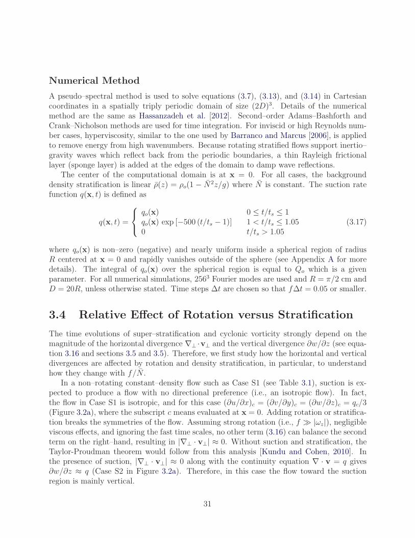
The center of the computational domain is at x = 0. For all cases, the backgrounddensity stratification is linear ρ(z) = ρo(1 − N2z/g) where N is constant. The suction ratefunction q(x, t) is defined as

q(x, t) =

⎧⎨⎩

qo(x) 0 ≤ t/ts ≤ 1qo(x) exp [−500 (t/ts − 1)] 1 < t/ts ≤ 1.050 t/ts > 1.05

(3.17)

where qo(x) is non–zero (negative) and nearly uniform inside a spherical region of radiusR centered at x = 0 and rapidly vanishes outside of the sphere (see Appendix A for moredetails). The integral of qo(x) over the spherical region is equal to Qo which is a givenparameter. For all numerical simulations, 2563 Fourier modes are used and R = π/2 cm andD = 20R, unless otherwise stated. Time steps Δt are chosen so that fΔt = 0.05 or smaller.

3.4 Relative Effect of Rotation versus Stratification

The time evolutions of super–stratification and cyclonic vorticity strongly depend on themagnitude of the horizontal divergence ∇⊥ ·v⊥ and the vertical divergence ∂w/∂z (see equa-tion 3.16 and sections 3.5 and 3.5). Therefore, we first study how the horizontal and verticaldivergences are affected by rotation and density stratification, in particular, to understandhow they change with f/N .

In a non–rotating constant–density flow such as Case S1 (see Table 3.1), suction is ex-pected to produce a flow with no directional preference (i.e., an isotropic flow). In fact,the flow in Case S1 is isotropic, and for this case (∂u/∂x)c = (∂v/∂y)c = (∂w/∂z)c = qc/3(Figure 3.2a), where the subscript c means evaluated at x = 0. Adding rotation or stratifica-tion breaks the symmetries of the flow. Assuming strong rotation (i.e., f |ωz|), negligibleviscous effects, and ignoring the fast time scales, no other term (3.16) can balance the secondterm on the right–hand, resulting in |∇⊥ · v⊥| ≈ 0. Without suction and stratification, theTaylor-Proudman theorem would follow from this analysis [Kundu and Cohen, 2010]. Inthe presence of suction, |∇⊥ · v⊥| ≈ 0 along with the continuity equation ∇ · v = q gives∂w/∂z ≈ q (Case S2 in Figure 3.2a). Therefore, in this case the flow toward the suctionregion is mainly vertical.

31

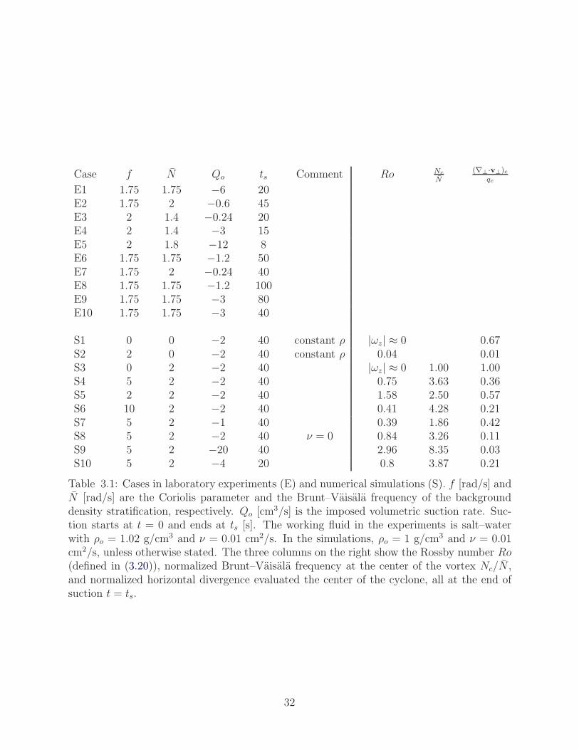
Case f N Qo ts Comment Ro Nc

N(∇⊥·v⊥)c

qc

E1 1.75 1.75 −6 20E2 1.75 2 −0.6 45E3 2 1.4 −0.24 20E4 2 1.4 −3 15E5 2 1.8 −12 8E6 1.75 1.75 −1.2 50E7 1.75 2 −0.24 40E8 1.75 1.75 −1.2 100E9 1.75 1.75 −3 80E10 1.75 1.75 −3 40

S1 0 0 −2 40 constant ρ |ωz| ≈ 0 0.67S2 2 0 −2 40 constant ρ 0.04 0.01S3 0 2 −2 40 |ωz| ≈ 0 1.00 1.00S4 5 2 −2 40 0.75 3.63 0.36S5 2 2 −2 40 1.58 2.50 0.57S6 10 2 −2 40 0.41 4.28 0.21S7 5 2 −1 40 0.39 1.86 0.42S8 5 2 −2 40 ν = 0 0.84 3.26 0.11S9 5 2 −20 40 2.96 8.35 0.03S10 5 2 −4 20 0.8 3.87 0.21

Table 3.1: Cases in laboratory experiments (E) and numerical simulations (S). f [rad/s] andN [rad/s] are the Coriolis parameter and the Brunt–Vaisala frequency of the backgrounddensity stratification, respectively. Qo [cm3/s] is the imposed volumetric suction rate. Suc-tion starts at t = 0 and ends at ts [s]. The working fluid in the experiments is salt–waterwith ρo = 1.02 g/cm3 and ν = 0.01 cm2/s. In the simulations, ρo = 1 g/cm3 and ν = 0.01cm2/s, unless otherwise stated. The three columns on the right show the Rossby number Ro(defined in (3.20)), normalized Brunt–Vaisala frequency at the center of the vortex Nc/N ,and normalized horizontal divergence evaluated the center of the cyclone, all at the end ofsuction t = ts.

32

0 0.2 0.4 0.6 0.8 1−0.2

0

0.2

0.4

0.6

0.8

1

t/ts(a)

0 0.2 0.4 0.6 0.8 1−0.2

0

0.2

0.4

0.6

0.8

1

t/ts(b)

Figure 3.2: Effect of rotation and stratification on the divergence of the velocity field duringsuction. The solid lines show the normalized horizontal divergence ((∇⊥ · v⊥)/q)c and thebroken lines show the normalized vertical divergence ((∂w/∂z)/q)c. (a) The flow in Case S1(blue, no symbol) is non–rotating (f = 0) and constant–density and has ((∇⊥ ·v⊥)/q)c = 2/3and ((∂w/∂z)/q)c = 1/3. The vertical divergence ∂w/∂z dominates in Cases S2 (red •) whichis rotating and constant–density. The flow in Case S3 (black �) is non–rotating (f = 0) andstratified, and has a dominant horizontal divergence. (b) Case S4 has f/N = 2.5 (blue, nosymbol), Case S5 has f/N = 1 (red •), and Case S6 has f/N = 5 (black �).

Strong stratification suppresses vertical motions and decouples the flow into horizontallayers [Kundu and Cohen, 2010]. As a result, for a non–rotating stratified flow such as CaseS3, we expect ∂w/∂z ≈ 0 and ∇⊥ · v⊥ ≈ q, which is observed in Figure 3.2a. Hence, theflow in this case approaches the suction region largely horizontally. Oscillations in Cases S2and S3 (Figure 3.2a) are due to the inertial and internal gravity waves, respectively.

In the presence of both rotation and stratification, the relative magnitude of the horizontaland vertical divergences depends on f/N . Figure 3.2b compares Cases S4–S6, which havef/N = 2.5, 1, and 5, respectively. As expected, a larger f/N results in a larger verticaldivergence |∂w/∂z| compared to the horizontal divergence |∇⊥ · v⊥|. This understanding ofthe role of f/N will be used in sections 3.5 and 3.5 and is consistent with the analyticalresults of McDonald [1992] for a point sink in rotating stratified flows (see his Figure 1).

33

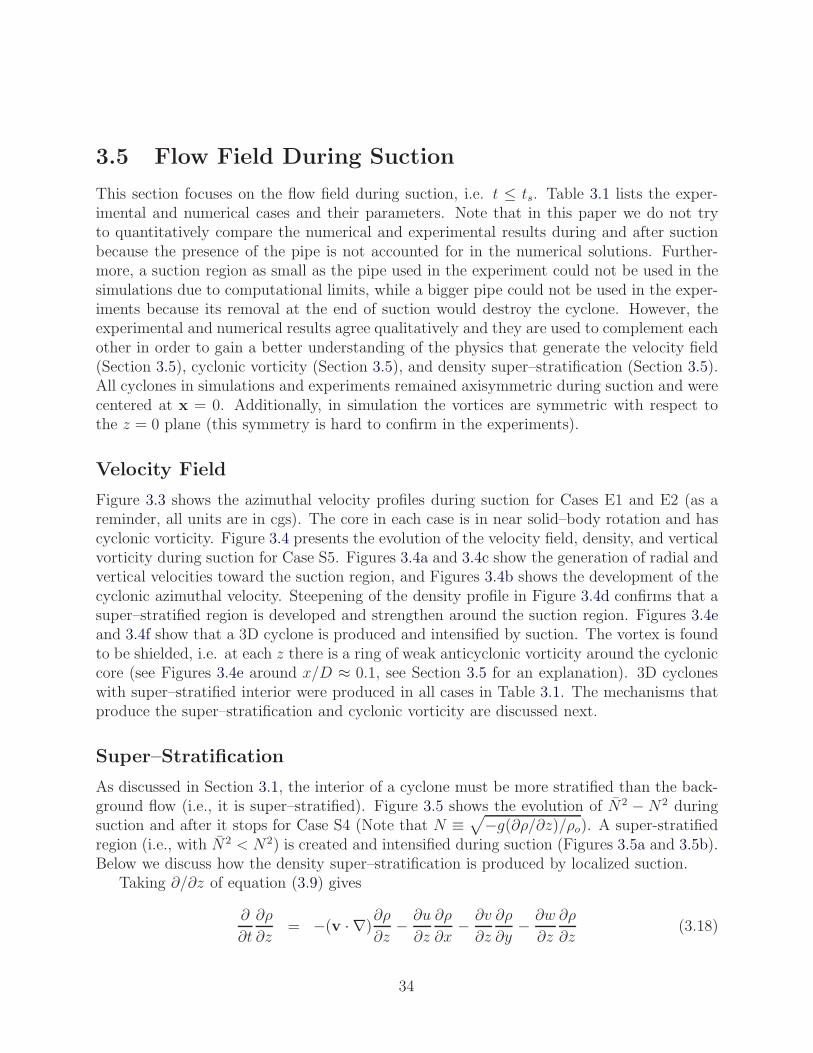
3.5 Flow Field During Suction

This section focuses on the flow field during suction, i.e. t ≤ ts. Table 3.1 lists the exper-imental and numerical cases and their parameters. Note that in this paper we do not tryto quantitatively compare the numerical and experimental results during and after suctionbecause the presence of the pipe is not accounted for in the numerical solutions. Further-more, a suction region as small as the pipe used in the experiment could not be used in thesimulations due to computational limits, while a bigger pipe could not be used in the exper-iments because its removal at the end of suction would destroy the cyclone. However, theexperimental and numerical results agree qualitatively and they are used to complement eachother in order to gain a better understanding of the physics that generate the velocity field(Section 3.5), cyclonic vorticity (Section 3.5), and density super–stratification (Section 3.5).All cyclones in simulations and experiments remained axisymmetric during suction and werecentered at x = 0. Additionally, in simulation the vortices are symmetric with respect tothe z = 0 plane (this symmetry is hard to confirm in the experiments).

Velocity Field

Figure 3.3 shows the azimuthal velocity profiles during suction for Cases E1 and E2 (as areminder, all units are in cgs). The core in each case is in near solid–body rotation and hascyclonic vorticity. Figure 3.4 presents the evolution of the velocity field, density, and verticalvorticity during suction for Case S5. Figures 3.4a and 3.4c show the generation of radial andvertical velocities toward the suction region, and Figures 3.4b shows the development of thecyclonic azimuthal velocity. Steepening of the density profile in Figure 3.4d confirms that asuper–stratified region is developed and strengthen around the suction region. Figures 3.4eand 3.4f show that a 3D cyclone is produced and intensified by suction. The vortex is foundto be shielded, i.e. at each z there is a ring of weak anticyclonic vorticity around the cycloniccore (see Figures 3.4e around x/D ≈ 0.1, see Section 3.5 for an explanation). 3D cycloneswith super–stratified interior were produced in all cases in Table 3.1. The mechanisms thatproduce the super–stratification and cyclonic vorticity are discussed next.

Super–Stratification

As discussed in Section 3.1, the interior of a cyclone must be more stratified than the back-ground flow (i.e., it is super–stratified). Figure 3.5 shows the evolution of N2 − N2 duringsuction and after it stops for Case S4 (Note that N ≡ √−g(∂ρ/∂z)/ρo). A super-stratifiedregion (i.e., with N2 < N2) is created and intensified during suction (Figures 3.5a and 3.5b).Below we discuss how the density super–stratification is produced by localized suction.

Taking ∂/∂z of equation (3.9) gives

∂

∂t

∂ρ

∂z= −(v · ∇)

∂ρ

∂z− ∂u

∂z

∂ρ

∂x− ∂v

∂z

∂ρ

∂y− ∂w

∂z

∂ρ

∂z(3.18)

34

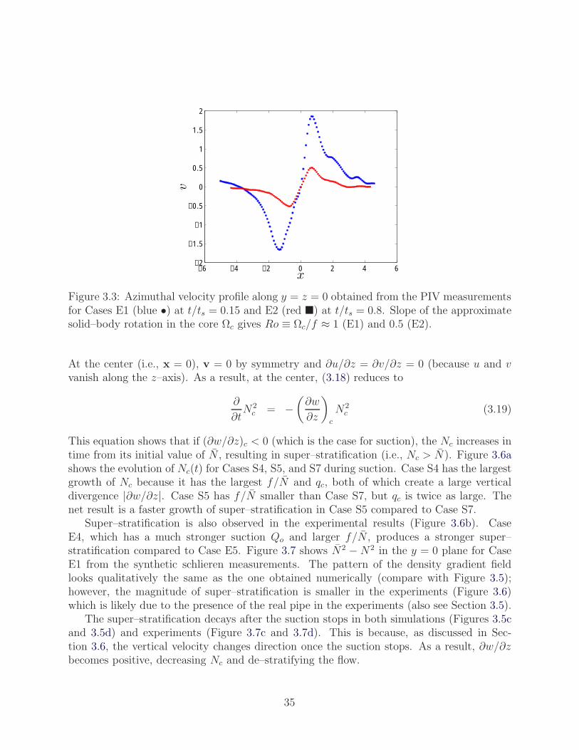
−6 −4 −2 0 2 4 6−2

−1.5

−1

−0.5

0

0.5

1

1.5

2

x

v

Figure 3.3: Azimuthal velocity profile along y = z = 0 obtained from the PIV measurementsfor Cases E1 (blue •) at t/ts = 0.15 and E2 (red �) at t/ts = 0.8. Slope of the approximatesolid–body rotation in the core Ωc gives Ro ≡ Ωc/f ≈ 1 (E1) and 0.5 (E2).

At the center (i.e., x = 0), v = 0 by symmetry and ∂u/∂z = ∂v/∂z = 0 (because u and vvanish along the z–axis). As a result, at the center, (3.18) reduces to

∂

∂tN2

c = −(∂w

∂z

)c

N2c (3.19)

This equation shows that if (∂w/∂z)c < 0 (which is the case for suction), the Nc increases intime from its initial value of N , resulting in super–stratification (i.e., Nc > N). Figure 3.6ashows the evolution of Nc(t) for Cases S4, S5, and S7 during suction. Case S4 has the largestgrowth of Nc because it has the largest f/N and qc, both of which create a large verticaldivergence |∂w/∂z|. Case S5 has f/N smaller than Case S7, but qc is twice as large. Thenet result is a faster growth of super–stratification in Case S5 compared to Case S7.

Super–stratification is also observed in the experimental results (Figure 3.6b). CaseE4, which has a much stronger suction Qo and larger f/N , produces a stronger super–stratification compared to Case E5. Figure 3.7 shows N2 − N2 in the y = 0 plane for CaseE1 from the synthetic schlieren measurements. The pattern of the density gradient fieldlooks qualitatively the same as the one obtained numerically (compare with Figure 3.5);however, the magnitude of super–stratification is smaller in the experiments (Figure 3.6)which is likely due to the presence of the real pipe in the experiments (also see Section 3.5).

The super–stratification decays after the suction stops in both simulations (Figures 3.5cand 3.5d) and experiments (Figure 3.7c and 3.7d). This is because, as discussed in Sec-tion 3.6, the vertical velocity changes direction once the suction stops. As a result, ∂w/∂zbecomes positive, decreasing Nc and de–stratifying the flow.

35

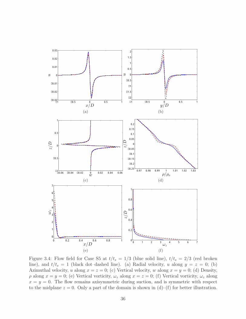
−1 −0.5 0 0.5 1−0.03

−0.02

−0.01

0

0.01

0.02

0.03

x/D

u

(a)

−1 −0.5 0 0.5 1

−2

−1.5

−1

−0.5

0

0.5

1

1.5

2

y/D

u

(b)

−0.06 −0.04 −0.02 0 0.02 0.04 0.06−1

−0.5

0

0.5

1

w

z/D

(c)

0.97 0.98 0.99 1 1.01 1.02 1.03−0.25

−0.2

−0.15

−0.1

−0.05

0

0.05

0.1

0.15

0.2

ρ/ρo

z/D

(d)

0 0.2 0.4 0.6 0.8 10

1

2

3

4

5

6

7

x/D

ωz

(e)

0 1 2 3 4 5 6 70

0.2

0.4

0.6

0.8

1

ωz

z/D

(f)

Figure 3.4: Flow field for Case S5 at t/ts = 1/3 (blue solid line), t/ts = 2/3 (red brokenline), and t/ts = 1 (black dot–dashed line). (a) Radial velocity, u along y = z = 0; (b)Azimuthal velocity, u along x = z = 0; (c) Vertical velocity, w along x = y = 0; (d) Density,ρ along x = y = 0; (e) Vertical vorticity, ωz along x = z = 0; (f) Vertical vorticity, ωz alongx = y = 0. The flow remains axisymmetric during suction, and is symmetric with respectto the midplane z = 0. Only a part of the domain is shown in (d)–(f) for better illustration.

36

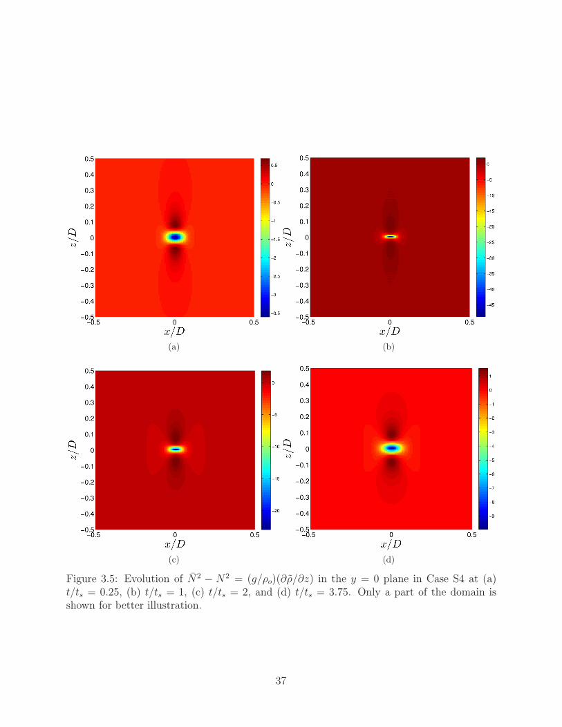
(a) (b)

(c) (d)

Figure 3.5: Evolution of N2 − N2 = (g/ρo)(∂ρ/∂z) in the y = 0 plane in Case S4 at (a)t/ts = 0.25, (b) t/ts = 1, (c) t/ts = 2, and (d) t/ts = 3.75. Only a part of the domain isshown for better illustration.

37

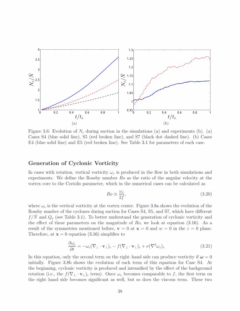
0 0.2 0.4 0.6 0.8 11

1.5

2

2.5

3

3.5

4

t/ts

Nc/N

(a)

0 0.2 0.4 0.6 0.8 10.95

1

1.05

1.1

1.15

1.2

1.25

1.3

t/tsN

c/N

(b)

Figure 3.6: Evolution of Nc during suction in the simulations (a) and experiments (b). (a)Cases S4 (blue solid line), S5 (red broken line), and S7 (black dot–dashed line). (b) CasesE4 (blue solid line) and E5 (red broken line). See Table 3.1 for parameters of each case.

Generation of Cyclonic Vorticity

In cases with rotation, vertical vorticity ωz is produced in the flow in both simulations andexperiments. We define the Rossby number Ro as the ratio of the angular velocity at thevortex core to the Coriolis parameter, which in the numerical cases can be calculated as

Ro ≡ ωc

2f, (3.20)

where ωc is the vertical vorticity at the vortex center. Figure 3.8a shows the evolution of theRossby number of the cyclones during suction for Cases S4, S5, and S7, which have differentf/N and Qo (see Table 3.1). To better understand the generation of cyclonic vorticity andthe effect of these parameters on the magnitude of Ro, we look at equation (3.16). As aresult of the symmetries mentioned before, v = 0 at x = 0 and w = 0 in the z = 0 plane.Therefore, at x = 0 equation (3.16) simplifies to

∂ωc

∂t= −ωc(∇⊥ · v⊥)c − f(∇⊥ · v⊥)c + ν(∇2ωz)c (3.21)

In this equation, only the second term on the right–hand side can produce vorticity if ω = 0initially. Figure 3.8b shows the evolution of each term of this equation for Case S4. Atthe beginning, cyclonic vorticity is produced and intensified by the effect of the backgroundrotation (i.e., the f(∇⊥ · v⊥)c term). Once ωc becomes comparable to f , the first term onthe right–hand side becomes significant as well, but so does the viscous term. These two

38

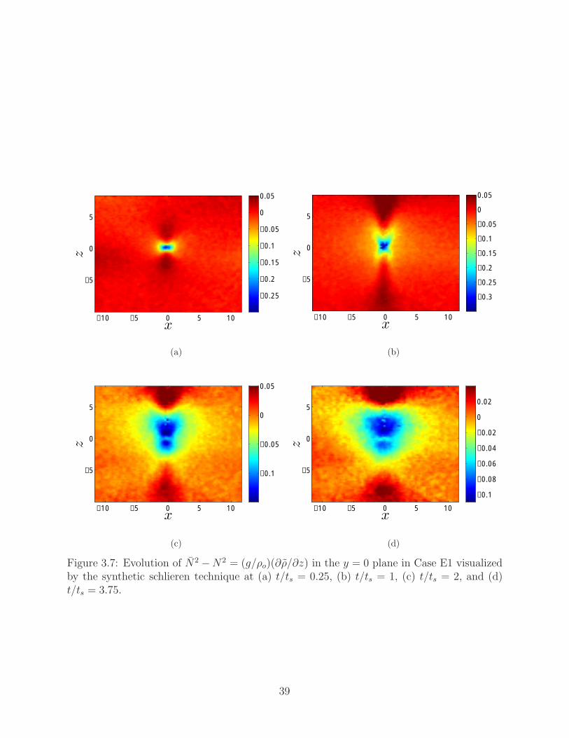
x

z

−10 −5 0 5 10

−5

0

5

−0.25

−0.2

−0.15

−0.1

−0.05

0

0.05

(a)

x

z

−10 −5 0 5 10

−5

0

5

−0.3

−0.25

−0.2

−0.15

−0.1

−0.05

0

0.05

(b)

x

z

−10 −5 0 5 10

−5

0

5

−0.1

−0.05

0

0.05

(c)

x

z

−10 −5 0 5 10

−5

0

5

−0.1

−0.08

−0.06

−0.04

−0.02

0

0.02

(d)

Figure 3.7: Evolution of N2 −N2 = (g/ρo)(∂ρ/∂z) in the y = 0 plane in Case E1 visualizedby the synthetic schlieren technique at (a) t/ts = 0.25, (b) t/ts = 1, (c) t/ts = 2, and (d)t/ts = 3.75.

39

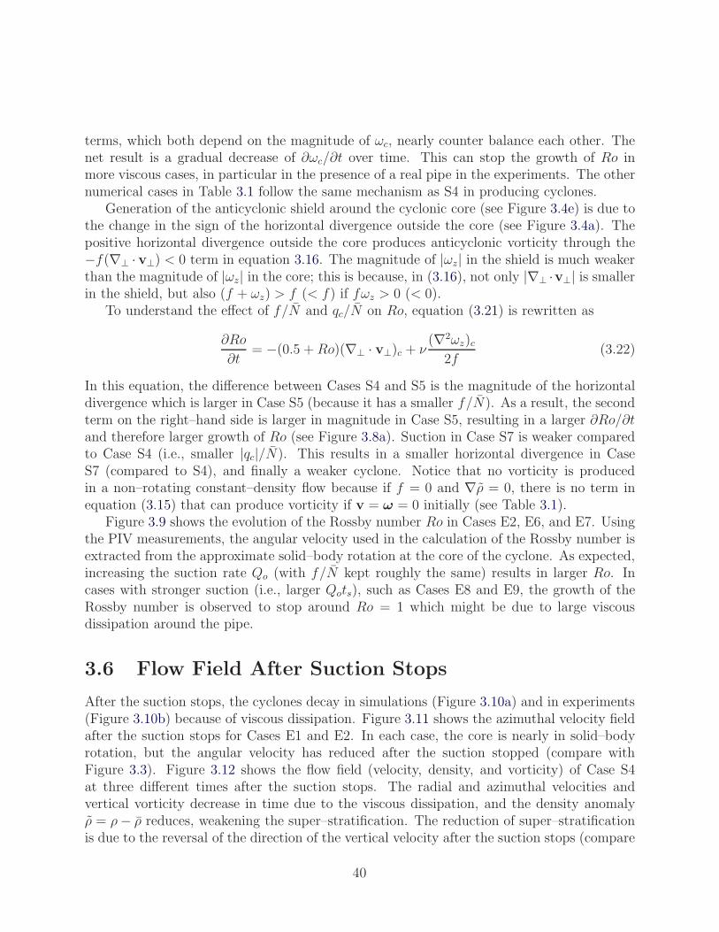
terms, which both depend on the magnitude of ωc, nearly counter balance each other. Thenet result is a gradual decrease of ∂ωc/∂t over time. This can stop the growth of Ro inmore viscous cases, in particular in the presence of a real pipe in the experiments. The othernumerical cases in Table 3.1 follow the same mechanism as S4 in producing cyclones.

Generation of the anticyclonic shield around the cyclonic core (see Figure 3.4e) is due tothe change in the sign of the horizontal divergence outside the core (see Figure 3.4a). Thepositive horizontal divergence outside the core produces anticyclonic vorticity through the−f(∇⊥ · v⊥) < 0 term in equation 3.16. The magnitude of |ωz| in the shield is much weakerthan the magnitude of |ωz| in the core; this is because, in (3.16), not only |∇⊥ ·v⊥| is smallerin the shield, but also (f + ωz) > f (< f) if fωz > 0 (< 0).

To understand the effect of f/N and qc/N on Ro, equation (3.21) is rewritten as

∂Ro

∂t= −(0.5 +Ro)(∇⊥ · v⊥)c + ν

(∇2ωz)c2f

(3.22)

In this equation, the difference between Cases S4 and S5 is the magnitude of the horizontaldivergence which is larger in Case S5 (because it has a smaller f/N). As a result, the secondterm on the right–hand side is larger in magnitude in Case S5, resulting in a larger ∂Ro/∂tand therefore larger growth of Ro (see Figure 3.8a). Suction in Case S7 is weaker comparedto Case S4 (i.e., smaller |qc|/N). This results in a smaller horizontal divergence in CaseS7 (compared to S4), and finally a weaker cyclone. Notice that no vorticity is producedin a non–rotating constant–density flow because if f = 0 and ∇ρ = 0, there is no term inequation (3.15) that can produce vorticity if v = ω = 0 initially (see Table 3.1).

Figure 3.9 shows the evolution of the Rossby number Ro in Cases E2, E6, and E7. Usingthe PIV measurements, the angular velocity used in the calculation of the Rossby number isextracted from the approximate solid–body rotation at the core of the cyclone. As expected,increasing the suction rate Qo (with f/N kept roughly the same) results in larger Ro. Incases with stronger suction (i.e., larger Qots), such as Cases E8 and E9, the growth of theRossby number is observed to stop around Ro = 1 which might be due to large viscousdissipation around the pipe.

3.6 Flow Field After Suction Stops

After the suction stops, the cyclones decay in simulations (Figure 3.10a) and in experiments(Figure 3.10b) because of viscous dissipation. Figure 3.11 shows the azimuthal velocity fieldafter the suction stops for Cases E1 and E2. In each case, the core is nearly in solid–bodyrotation, but the angular velocity has reduced after the suction stopped (compare withFigure 3.3). Figure 3.12 shows the flow field (velocity, density, and vorticity) of Case S4at three different times after the suction stops. The radial and azimuthal velocities andvertical vorticity decrease in time due to the viscous dissipation, and the density anomalyρ = ρ− ρ reduces, weakening the super–stratification. The reduction of super–stratificationis due to the reversal of the direction of the vertical velocity after the suction stops (compare

40

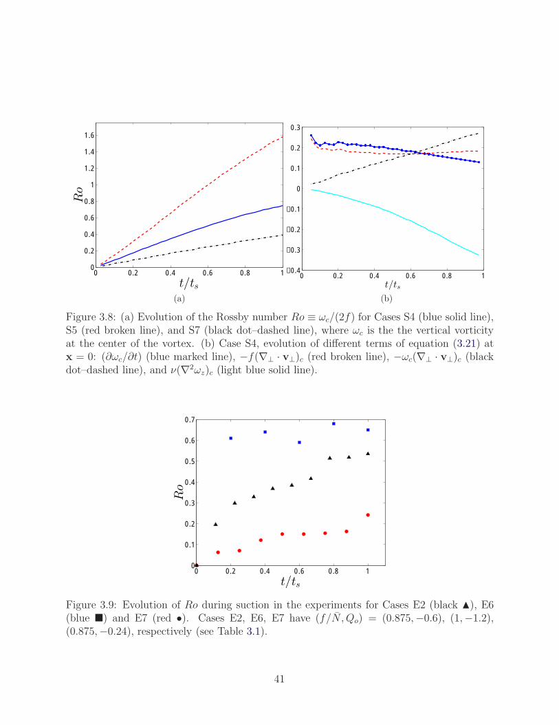
0 0.2 0.4 0.6 0.8 10

0.2

0.4

0.6

0.8

1

1.2

1.4

1.6

t/ts

Ro

(a)

0 0.2 0.4 0.6 0.8 1−0.4

−0.3

−0.2

−0.1

0

0.1

0.2

0.3

t/ts

(b)

Figure 3.8: (a) Evolution of the Rossby number Ro ≡ ωc/(2f) for Cases S4 (blue solid line),S5 (red broken line), and S7 (black dot–dashed line), where ωc is the the vertical vorticityat the center of the vortex. (b) Case S4, evolution of different terms of equation (3.21) atx = 0: (∂ωc/∂t) (blue marked line), −f(∇⊥ · v⊥)c (red broken line), −ωc(∇⊥ · v⊥)c (blackdot–dashed line), and ν(∇2ωz)c (light blue solid line).

0 0.2 0.4 0.6 0.8 10

0.1

0.2

0.3

0.4

0.5

0.6

0.7

t/ts

Ro

Figure 3.9: Evolution of Ro during suction in the experiments for Cases E2 (black �), E6(blue �) and E7 (red •). Cases E2, E6, E7 have (f/N, Qo) = (0.875,−0.6), (1,−1.2),(0.875,−0.24), respectively (see Table 3.1).

41

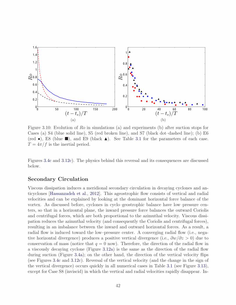
0 50 100 150 2000

0.2

0.4

0.6

0.8

1

1.2

1.4

1.6

(t− ts)/T

Ro

(a)

0 20 40 60 80 1000

0.2

0.4

0.6

0.8

1

(t− ts)/T

Ro

(b)

Figure 3.10: Evolution of Ro in simulations (a) and experiments (b) after suction stops forCases (a) S4 (blue solid line), S5 (red broken line), and S7 (black dot–dashed line); (b) E6(red •), E8 (blue �), and E9 (black �). See Table 3.1 for the parameters of each case.T = 4π/f is the inertial period.

Figures 3.4c and 3.12c). The physics behind this reversal and its consequences are discussedbelow.

Secondary Circulation

Viscous dissipation induces a meridional secondary circulation in decaying cyclones and an-ticyclones [Hassanzadeh et al., 2012]. This ageostrophic flow consists of vertical and radialvelocities and can be explained by looking at the dominant horizontal force balance of thevortex. As discussed before, cyclones in cyclo–geostrophic balance have low–pressure cen-ters, so that in a horizontal plane, the inward pressure force balances the outward Coriolisand centrifugal forces, which are both proportional to the azimuthal velocity. Viscous dissi-pation reduces the azimuthal velocity (and consequently the Coriolis and centrifugal forces),resulting in an imbalance between the inward and outward horizontal forces. As a result, aradial flow is induced toward the low–pressure center. A converging radial flow (i.e., nega-tive horizontal divergence) produces a positive vertical divergence (i.e., ∂w/∂z > 0) due toconservation of mass (notice that q = 0 now). Therefore, the direction of the radial flow ina viscously decaying cyclone (Figure 3.12a) is the same as the direction of the radial flowduring suction (Figure 3.4a); on the other hand, the direction of the vertical velocity flips(see Figures 3.4c and 3.12c). Reversal of the vertical velocity (and the change in the sign ofthe vertical divergence) occurs quickly in all numerical cases in Table 3.1 (see Figure 3.13),except for Case S8 (inviscid) in which the vertical and radial velocities rapidly disappear. In-

42

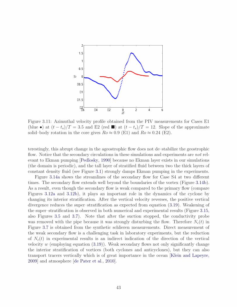
−6 −4 −2 0 2 4 6−2

−1.5

−1

−0.5

0

0.5

1

1.5

2

x

v

Figure 3.11: Azimuthal velocity profile obtained from the PIV measurements for Cases E1(blue •) at (t − ts)/T = 3.5 and E2 (red �) at (t − ts)/T = 12. Slope of the approximatesolid–body rotation in the core gives Ro ≈ 0.9 (E1) and Ro ≈ 0.24 (E2).

terestingly, this abrupt change in the ageostrophic flow does not de–stabilize the geostrophicflow. Notice that the secondary circulations in these simulations and experiments are not rel-evant to Ekman pumping [Pedlosky, 1990] because no Ekman layer exists in our simulations(the domain is periodic), and the tall layer of stratified fluid between two the thick layers ofconstant density fluid (see Figure 3.1) strongly damps Ekman pumping in the experiments.

Figure 3.14a shows the streamlines of the secondary flow for Case S4 at two differenttimes. The secondary flow extends well beyond the boundaries of the vortex (Figure 3.14b).As a result, even though the secondary flow is weak compared to the primary flow (compareFigures 3.12a and 3.12b), it plays an important role in the dynamics of the cyclone bychanging its interior stratification. After the vertical velocity reverses, the positive verticaldivergence reduces the super–stratification as expected from equation (3.19). Weakening ofthe super–stratification is observed in both numerical and experimental results (Figure 3.15,also Figures 3.5 and 3.7). Note that after the suction stopped, the conductivity probewas removed with the pipe because it was strongly disturbing the flow. Therefore Nc(t) inFigure 3.7 is obtained from the synthetic schlieren measurements. Direct measurement ofthe weak secondary flow is a challenging task in laboratory experiments, but the reductionof Nc(t) in experimental results is an indirect indication of the direction of the verticalvelocity w (employing equation (3.19)). Weak secondary flows not only significantly changethe interior stratification of vortices (both cyclones and anticyclones), but they can alsotransport tracers vertically which is of great importance in the ocean [Klein and Lapeyre,2009] and atmosphere [de Pater et al., 2010].

43

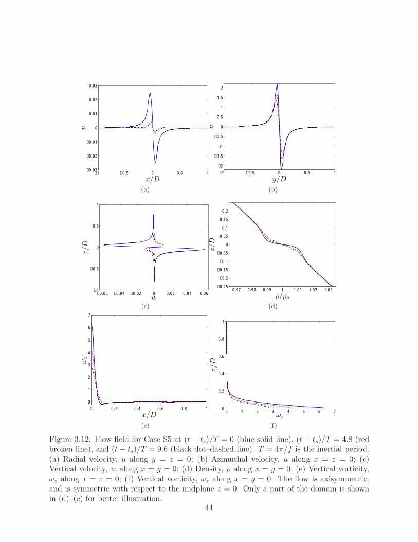
−1 −0.5 0 0.5 1−0.03

−0.02

−0.01

0

0.01

0.02

0.03

x/D

u

(a)

−1 −0.5 0 0.5 1

−2

−1.5

−1

−0.5

0

0.5

1

1.5

2

y/D

u

(b)

−0.06 −0.04 −0.02 0 0.02 0.04 0.06−1

−0.5

0

0.5

1

w

z/D

(c)

0.97 0.98 0.99 1 1.01 1.02 1.03−0.25

−0.2

−0.15

−0.1

−0.05

0

0.05

0.1

0.15

0.2

ρ/ρo

z/D

(d)

0 0.2 0.4 0.6 0.8 10

1

2

3

4

5

6

7

x/D

ωz

(e)

0 1 2 3 4 5 6 70

0.2

0.4

0.6

0.8

1

ωz

z/D

(f)

Figure 3.12: Flow field for Case S5 at (t− ts)/T = 0 (blue solid line), (t− ts)/T = 4.8 (redbroken line), and (t− ts)/T = 9.6 (black dot–dashed line). T = 4π/f is the inertial period.(a) Radial velocity, u along y = z = 0; (b) Azimuthal velocity, u along x = z = 0; (c)Vertical velocity, w along x = y = 0; (d) Density, ρ along x = y = 0; (e) Vertical vorticity,ωz along x = z = 0; (f) Vertical vorticity, ωz along x = y = 0. The flow is axisymmetric,and is symmetric with respect to the midplane z = 0. Only a part of the domain is shownin (d)–(e) for better illustration.

44

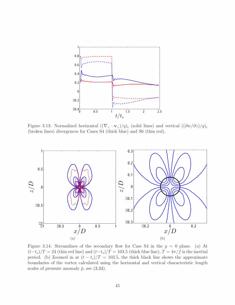
0 0.5 1 1.5 2 2.5−0.4

−0.2

0

0.2

0.4

0.6

0.8

1

t/ts

Figure 3.13: Normalized horizontal ((∇⊥ · v⊥)/q)c (solid lines) and vertical ((∂w/∂z)/q)c(broken lines) divergences for Cases S4 (thick blue) and S6 (thin red).

−1 −0.5 0 0.5 1−1

−0.5

0

0.5

1

x/D

z/D

(a)

−0.2 0 0.2−0.3

−0.2

−0.1

0

0.1

0.2

0.3

x/D

z/D

(b)

Figure 3.14: Streamlines of the secondary flow for Case S4 in the y = 0 plane. (a) At(t−ts)/T = 24 (thin red line) and (t−ts)/T = 103.5 (thick blue line), T = 4π/f is the inertialperiod. (b) Zoomed in at (t − ts)/T = 103.5, the thick black line shows the approximateboundaries of the vortex calculated using the horizontal and vertical characteristic lengthscales of pressure anomaly p, see (3.24).

45

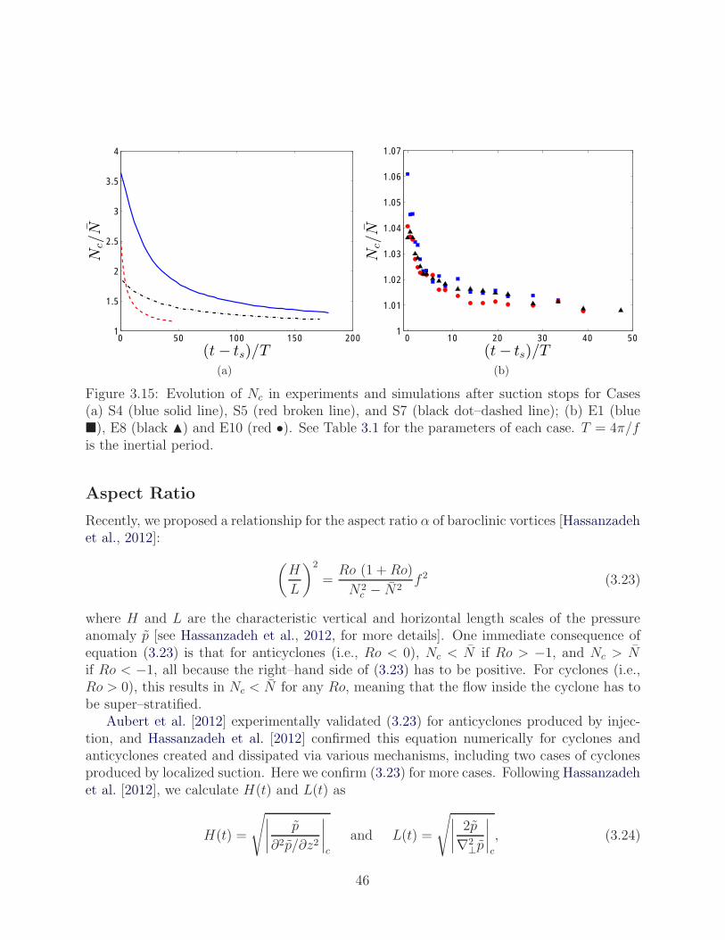
0 50 100 150 2001

1.5

2

2.5

3

3.5

4

(t − ts)/T

Nc/N

(a)

0 10 20 30 40 501

1.01

1.02

1.03

1.04

1.05

1.06

1.07

(t− ts)/T

Nc/N

(b)

Figure 3.15: Evolution of Nc in experiments and simulations after suction stops for Cases(a) S4 (blue solid line), S5 (red broken line), and S7 (black dot–dashed line); (b) E1 (blue�), E8 (black �) and E10 (red •). See Table 3.1 for the parameters of each case. T = 4π/fis the inertial period.

Aspect Ratio

Recently, we proposed a relationship for the aspect ratio α of baroclinic vortices [Hassanzadehet al., 2012]: (

H

L

)2

=Ro (1 +Ro)

N2c − N2

f 2 (3.23)

where H and L are the characteristic vertical and horizontal length scales of the pressureanomaly p [see Hassanzadeh et al., 2012, for more details]. One immediate consequence ofequation (3.23) is that for anticyclones (i.e., Ro < 0), Nc < N if Ro > −1, and Nc > Nif Ro < −1, all because the right–hand side of (3.23) has to be positive. For cyclones (i.e.,Ro > 0), this results in Nc < N for any Ro, meaning that the flow inside the cyclone has tobe super–stratified.

Aubert et al. [2012] experimentally validated (3.23) for anticyclones produced by injec-tion, and Hassanzadeh et al. [2012] confirmed this equation numerically for cyclones andanticyclones created and dissipated via various mechanisms, including two cases of cyclonesproduced by localized suction. Here we confirm (3.23) for more cases. Following Hassanzadehet al. [2012], we calculate H(t) and L(t) as

H(t) =

√∣∣∣∣ p

∂2p/∂z2

∣∣∣∣c

and L(t) =

√∣∣∣∣ 2p

∇2⊥p

∣∣∣∣c

, (3.24)

46

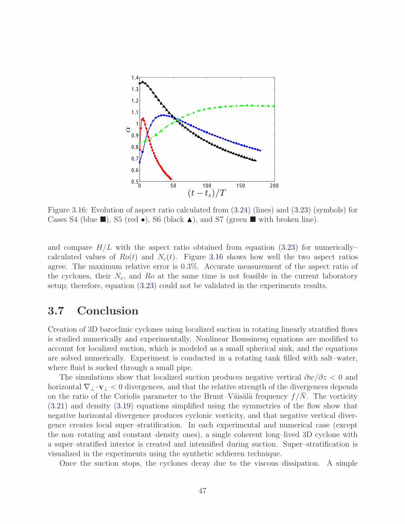
0 50 100 150 2000.5

0.6

0.7

0.8

0.9

1

1.1

1.2

1.3

1.4

(t− ts)/T

α

Figure 3.16: Evolution of aspect ratio calculated from (3.24) (lines) and (3.23) (symbols) forCases S4 (blue �), S5 (red •), S6 (black �), and S7 (green � with broken line).

and compare H/L with the aspect ratio obtained from equation (3.23) for numerically–calculated values of Ro(t) and Nc(t). Figure 3.16 shows how well the two aspect ratiosagree. The maximum relative error is 0.3%. Accurate measurement of the aspect ratio ofthe cyclones, their Nc, and Ro at the same time is not feasible in the current laboratorysetup; therefore, equation (3.23) could not be validated in the experiments results.

3.7 Conclusion

Creation of 3D baroclinic cyclones using localized suction in rotating linearly stratified flowsis studied numerically and experimentally. Nonlinear Boussinesq equations are modified toaccount for localized suction, which is modeled as a small spherical sink, and the equationsare solved numerically. Experiment is conducted in a rotating tank filled with salt–water,where fluid is sucked through a small pipe.

The simulations show that localized suction produces negative vertical ∂w/∂z < 0 andhorizontal ∇⊥ ·v⊥ < 0 divergences, and that the relative strength of the divergences dependson the ratio of the Coriolis parameter to the Brunt–Vaisala frequency f/N . The vorticity(3.21) and density (3.19) equations simplified using the symmetries of the flow show thatnegative horizontal divergence produces cyclonic vorticity, and that negative vertical diver-gence creates local super–stratification. In each experimental and numerical case (exceptthe non–rotating and constant–density ones), a single coherent long–lived 3D cyclone witha super–stratified interior is created and intensified during suction. Super–stratification isvisualized in the experiments using the synthetic schlieren technique.

Once the suction stops, the cyclones decay due to the viscous dissipation. A simple

47

physical argument is given on why a viscously decaying cyclone has a secondary circulation(i.e., non–zero vertical and radial velocity) with ∂w/∂z > 0 and ∇⊥ · v⊥ < 0. Therefore,the vertical velocity is expected to reverse once the cyclone starts to decay. The reversalis observed in the numerical results. Although the secondary circulation is much weakerthan the cyclo–geostrophic flow, its role in the dynamics of the cyclone is significant. Thevertical velocity with positive divergence mixes the flow inside and outside of the cycloneand reduces the super—stratification (as evident from (3.19)). Measuring the secondaryflow is challenging in the laboratory, but the weakening of the super–stratification in theexperimental results is an indirect evidence of the reversal of the vertical velocity.

This paper provides a better understanding of the physics of the flows produced by lo-calized suction in rotating stratified flows, the mechanisms that create cyclonic vorticity andlocal super–stratification, and the secondary circulation of viscously decaying 3D barocliniccyclones. This understanding can be applied later to design and conduct well–controlledexperimental studies of cyclone–anticyclone asymmetry, and in particular the implicationsof this asymmetry for the stability, longevity, and secondary circulation of geophysical andastrophysical vortices. In addition, the role of the secondary circulation in the dynamics of3D vortices, especially its effect on their internal stratification and longevity, merits furthernumerical and experimental investigation.

48

49

Chapter 4

Self–Replicating 3D Vortices inStably–Stratified Rotating Shear

4.1 Introduction

For a protostar to accrete gas from its surrounding protoplanetary disk (PPD) [Armitage,2011] and grow into a star, the PPD must have an instability capable of transporting an-gular momentum radially outward [Balbus and Hawley, 1998]. This requirement has led toan intense effort to find instabilities in PPDs and other rotating flows in which the angularmomentum satisfies Rayleigh’s criterion for centrifugal stability, i.e., the absolute value ofthe angular momentum increases with increasing radius [Rayleigh, 1917]. Numerical studies[Balbus et al., 1996, Shen et al., 2006] of ideal gases in PPDs and experimental studies [Jiet al., 2006] of constant density fluids in rotating flows where the velocity obeys Rayleigh’scriterion show that the flows are both linearly and finite-amplitude stable to hydrodynamicperturbations. In regions of a PPD where the gas is sufficiently ionized to couple to mag-netic fields, the magneto-rotational instability (MRI) [Balbus and Hawley, 1998] can oper-ate. However, large regions of PPDs, known as dead zones, are too cool to ionize sufficientlyand have MRI. Strato-rotational instabilities [Le Bars and Le Gal, 2007] and Rossby waveinstabilities [Lovelace et al., 1999] could de-stabilize a PPD, but they require unrealistic im-permeable radial boundaries on the PPD or a large continually-forced density perturbation,respectively. Thus, star formation remains problematic.

Here we report a new type of finite-amplitude instability that occurs in neutrally-stable,shearing flows with stably-stratified densities (as in a PPD) and with velocities that wouldsatisfy Rayleigh’s stability criterion if the densities were constant – as assumed in Rayleigh’s

With minor modifications, Chapter 3 appears in:P. S. Marcus, S. Pei, C–H Jiang, and P. Hassanzadeh, Self–Replicating Three–Dimensional Vortices inNeutrally-Stable Stratified Rotating Shear Flows, submitted to the Physical Review Letters, 2013.

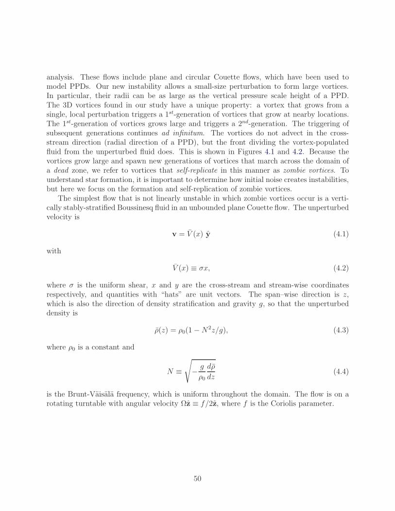
analysis. These flows include plane and circular Couette flows, which have been used tomodel PPDs. Our new instability allows a small-size perturbation to form large vortices.In particular, their radii can be as large as the vertical pressure scale height of a PPD.The 3D vortices found in our study have a unique property: a vortex that grows from asingle, local perturbation triggers a 1st-generation of vortices that grow at nearby locations.The 1st-generation of vortices grows large and triggers a 2nd-generation. The triggering ofsubsequent generations continues ad infinitum. The vortices do not advect in the cross-stream direction (radial direction of a PPD), but the front dividing the vortex-populatedfluid from the unperturbed fluid does. This is shown in Figures 4.1 and 4.2. Because thevortices grow large and spawn new generations of vortices that march across the domain ofa dead zone, we refer to vortices that self-replicate in this manner as zombie vortices. Tounderstand star formation, it is important to determine how initial noise creates instabilities,but here we focus on the formation and self-replication of zombie vortices.

The simplest flow that is not linearly unstable in which zombie vortices occur is a verti-cally stably-stratified Boussinesq fluid in an unbounded plane Couette flow. The unperturbedvelocity is

v = V (x) y (4.1)

with

V (x) ≡ σx, (4.2)

where σ is the uniform shear, x and y are the cross-stream and stream-wise coordinatesrespectively, and quantities with “hats” are unit vectors. The span–wise direction is z,which is also the direction of density stratification and gravity g, so that the unperturbeddensity is

ρ(z) = ρ0(1−N2z/g), (4.3)

where ρ0 is a constant and

N ≡√− g

ρ0

dρ

dz(4.4)

is the Brunt-Vaisala frequency, which is uniform throughout the domain. The flow is on arotating turntable with angular velocity Ωz ≡ f/2z, where f is the Coriolis parameter.

50

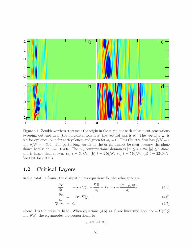
Figure 4.1: Zombie vortices start near the origin in the x–y plane with subsequent generationssweeping outward in x (the horizontal axis is x, the vertical axis is y). The vorticity ωz isred for cyclones; blue for anticyclones; and green for ωz = 0. This Couette flow has f/N = 1and σ/N = −3/4. The perturbing vortex at the origin cannot be seen because the planeshown here is at z = −0.404. The x-y computational domain is |x| ≤ 4.7124; |y| ≤ 2.3562,and is larger than shown. (a) t = 64/N . (b) t = 256/N . (c) t = 576/N . (d) t = 2240/N .See text for details.

4.2 Critical Layers

In the rotating frame, the dissipationless equations for the velocity v are:

∂v

∂t= −(v · ∇)v − ∇Π

ρ0+ fv × z− (ρ− ρ0)g

ρ0z (4.5)

∂ρ

∂t= −(v · ∇)ρ (4.6)

∇ · v = 0, (4.7)

where Π is the pressure head. When equations (4.5)–(4.7) are linearized about v = V (x) yand ρ(z), the eigenmodes are proportional to

ei(kyy+kzz−st),

51

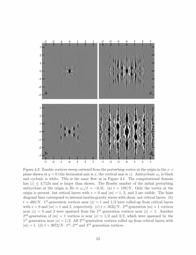
Figure 4.2: Zombie vortices sweep outward from the perturbing vortex at the origin in the x–zplane shown at y = 0 (the horizontal axis is x, the vertical axis is z). Anticyclonic ωz is blackand cyclonic is white. This is the same flow as in Figure 4.1. The computational domainhas |z| ≤ 4.7124 and is larger than shown. The Rossby number of the initial perturbinganticyclone at the origin is Ro ≡ ωz/f = −0.31. (a) t = 128/N . Only the vortex at theorigin is present, but critical layers with s = 0 and |m| = 1, 2, and 3 are visible. The faintdiagonal lines correspond to internal inertia-gravity waves with shear, not critical layers. (b)t = 480/N . 1st-generation vortices near |x| = 1 and 1/2 have rolled-up from critical layerswith s = 0 and |m| = 1 and 2, respectively. (c) t = 1632/N . 2nd-generation |m| = 1 vorticesnear |x| = 0 and 2 were spawned from the 1st generation vortices near |x| = 1. Another2nd-generation of |m| = 1 vortices is near |x| � 1/2 and 3/2, which were spawned by the1st generation near |x| = 1/2. All 2nd-generation vortices rolled up from critical layers with|m| = 1. (d) t = 3072/N . 1st, 2nd and 3rd generation vortices.

52

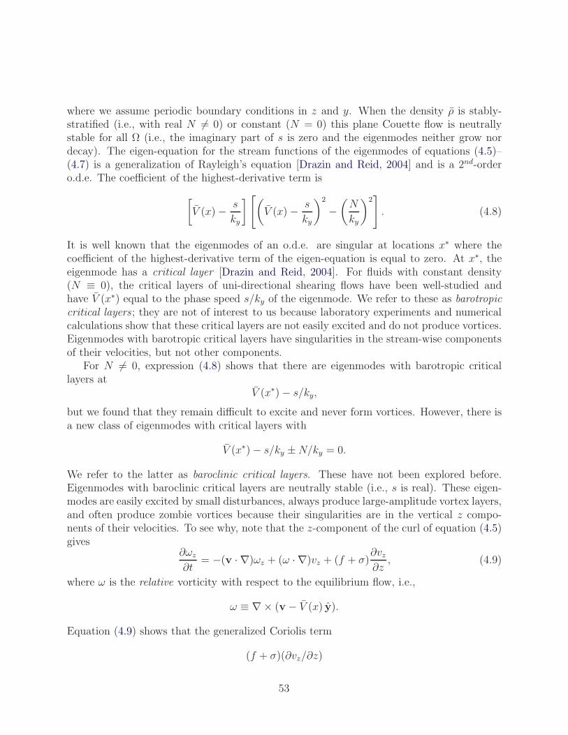
where we assume periodic boundary conditions in z and y. When the density ρ is stably-stratified (i.e., with real N �= 0) or constant (N = 0) this plane Couette flow is neutrallystable for all Ω (i.e., the imaginary part of s is zero and the eigenmodes neither grow nordecay). The eigen-equation for the stream functions of the eigenmodes of equations (4.5)–(4.7) is a generalization of Rayleigh’s equation [Drazin and Reid, 2004] and is a 2nd-ordero.d.e. The coefficient of the highest-derivative term is[

V (x)− s

ky

][(V (x)− s

ky

)2

−(N

ky

)2]. (4.8)

It is well known that the eigenmodes of an o.d.e. are singular at locations x∗ where thecoefficient of the highest-derivative term of the eigen-equation is equal to zero. At x∗, theeigenmode has a critical layer [Drazin and Reid, 2004]. For fluids with constant density(N ≡ 0), the critical layers of uni-directional shearing flows have been well-studied andhave V (x∗) equal to the phase speed s/ky of the eigenmode. We refer to these as barotropiccritical layers; they are not of interest to us because laboratory experiments and numericalcalculations show that these critical layers are not easily excited and do not produce vortices.Eigenmodes with barotropic critical layers have singularities in the stream-wise componentsof their velocities, but not other components.

For N �= 0, expression (4.8) shows that there are eigenmodes with barotropic criticallayers at

V (x∗)− s/ky,

but we found that they remain difficult to excite and never form vortices. However, there isa new class of eigenmodes with critical layers with

V (x∗)− s/ky ±N/ky = 0.

We refer to the latter as baroclinic critical layers. These have not been explored before.Eigenmodes with baroclinic critical layers are neutrally stable (i.e., s is real). These eigen-modes are easily excited by small disturbances, always produce large-amplitude vortex layers,and often produce zombie vortices because their singularities are in the vertical z compo-nents of their velocities. To see why, note that the z-component of the curl of equation (4.5)gives

∂ωz

∂t= −(v · ∇)ωz + (ω · ∇)vz + (f + σ)

∂vz∂z

, (4.9)

where ω is the relative vorticity with respect to the equilibrium flow, i.e.,

ω ≡ ∇× (v− V (x) y).

Equation (4.9) shows that the generalized Coriolis term

(f + σ)(∂vz/∂z)

53

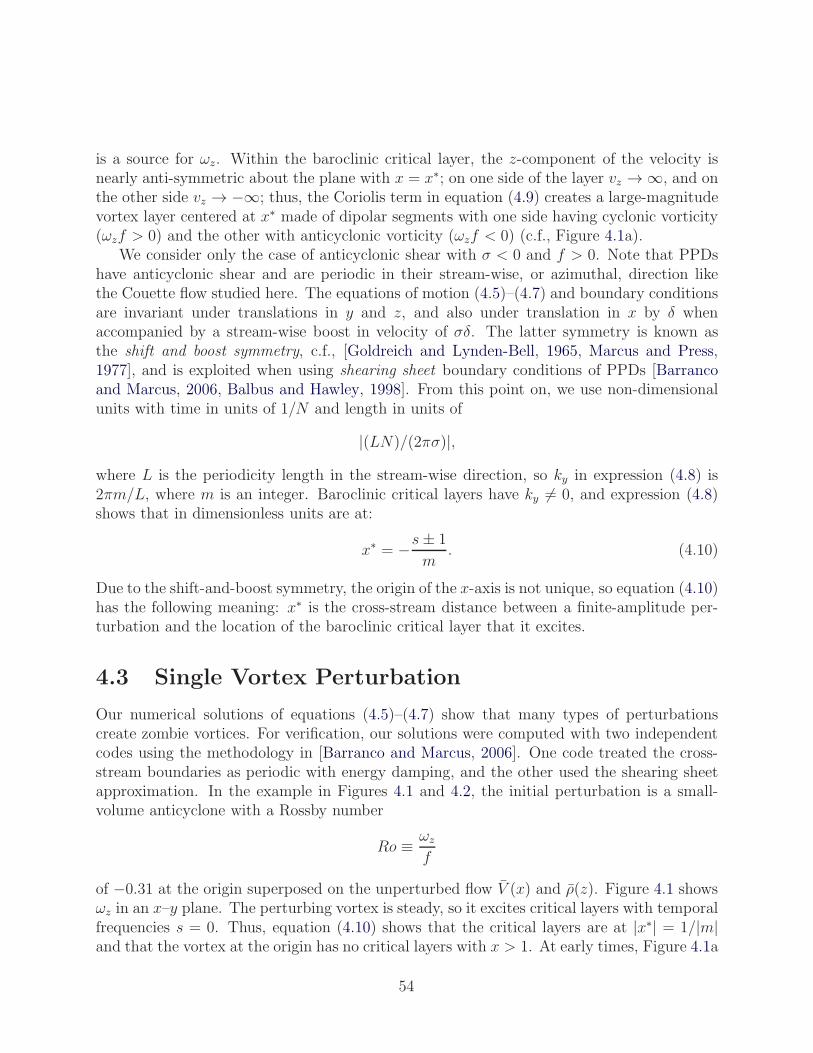
is a source for ωz. Within the baroclinic critical layer, the z-component of the velocity isnearly anti-symmetric about the plane with x = x∗; on one side of the layer vz → ∞, and onthe other side vz → −∞; thus, the Coriolis term in equation (4.9) creates a large-magnitudevortex layer centered at x∗ made of dipolar segments with one side having cyclonic vorticity(ωzf > 0) and the other with anticyclonic vorticity (ωzf < 0) (c.f., Figure 4.1a).

We consider only the case of anticyclonic shear with σ < 0 and f > 0. Note that PPDshave anticyclonic shear and are periodic in their stream-wise, or azimuthal, direction likethe Couette flow studied here. The equations of motion (4.5)–(4.7) and boundary conditionsare invariant under translations in y and z, and also under translation in x by δ whenaccompanied by a stream-wise boost in velocity of σδ. The latter symmetry is known asthe shift and boost symmetry, c.f., [Goldreich and Lynden-Bell, 1965, Marcus and Press,1977], and is exploited when using shearing sheet boundary conditions of PPDs [Barrancoand Marcus, 2006, Balbus and Hawley, 1998]. From this point on, we use non-dimensionalunits with time in units of 1/N and length in units of

|(LN)/(2πσ)|,where L is the periodicity length in the stream-wise direction, so ky in expression (4.8) is2πm/L, where m is an integer. Baroclinic critical layers have ky �= 0, and expression (4.8)shows that in dimensionless units are at:

x∗ = −s± 1

m. (4.10)

Due to the shift-and-boost symmetry, the origin of the x-axis is not unique, so equation (4.10)has the following meaning: x∗ is the cross-stream distance between a finite-amplitude per-turbation and the location of the baroclinic critical layer that it excites.

4.3 Single Vortex Perturbation

Our numerical solutions of equations (4.5)–(4.7) show that many types of perturbationscreate zombie vortices. For verification, our solutions were computed with two independentcodes using the methodology in [Barranco and Marcus, 2006]. One code treated the cross-stream boundaries as periodic with energy damping, and the other used the shearing sheetapproximation. In the example in Figures 4.1 and 4.2, the initial perturbation is a small-volume anticyclone with a Rossby number

Ro ≡ ωz

f

of −0.31 at the origin superposed on the unperturbed flow V (x) and ρ(z). Figure 4.1 showsωz in an x–y plane. The perturbing vortex is steady, so it excites critical layers with temporalfrequencies s = 0. Thus, equation (4.10) shows that the critical layers are at |x∗| = 1/|m|and that the vortex at the origin has no critical layers with x > 1. At early times, Figure 4.1a

54

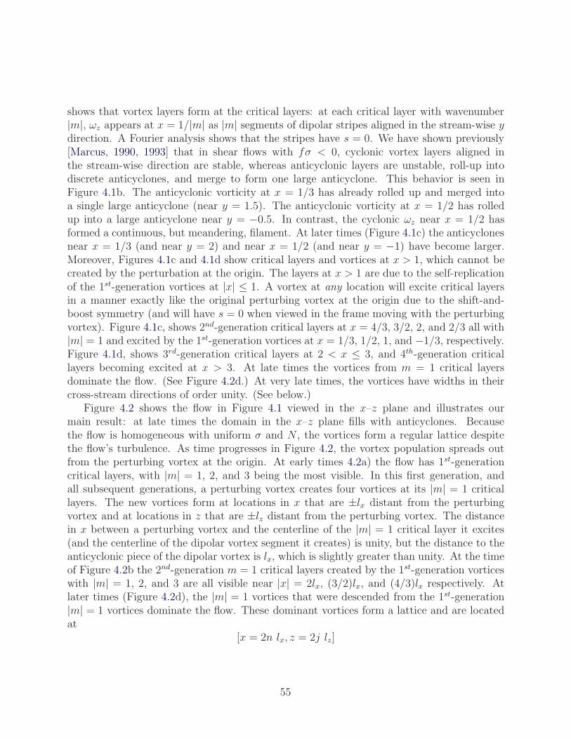
shows that vortex layers form at the critical layers: at each critical layer with wavenumber|m|, ωz appears at x = 1/|m| as |m| segments of dipolar stripes aligned in the stream-wise ydirection. A Fourier analysis shows that the stripes have s = 0. We have shown previously[Marcus, 1990, 1993] that in shear flows with fσ < 0, cyclonic vortex layers aligned inthe stream-wise direction are stable, whereas anticyclonic layers are unstable, roll-up intodiscrete anticyclones, and merge to form one large anticyclone. This behavior is seen inFigure 4.1b. The anticyclonic vorticity at x = 1/3 has already rolled up and merged intoa single large anticyclone (near y = 1.5). The anticyclonic vorticity at x = 1/2 has rolledup into a large anticyclone near y = −0.5. In contrast, the cyclonic ωz near x = 1/2 hasformed a continuous, but meandering, filament. At later times (Figure 4.1c) the anticyclonesnear x = 1/3 (and near y = 2) and near x = 1/2 (and near y = −1) have become larger.Moreover, Figures 4.1c and 4.1d show critical layers and vortices at x > 1, which cannot becreated by the perturbation at the origin. The layers at x > 1 are due to the self-replicationof the 1st-generation vortices at |x| ≤ 1. A vortex at any location will excite critical layersin a manner exactly like the original perturbing vortex at the origin due to the shift-and-boost symmetry (and will have s = 0 when viewed in the frame moving with the perturbingvortex). Figure 4.1c, shows 2nd-generation critical layers at x = 4/3, 3/2, 2, and 2/3 all with|m| = 1 and excited by the 1st-generation vortices at x = 1/3, 1/2, 1, and −1/3, respectively.Figure 4.1d, shows 3rd-generation critical layers at 2 < x ≤ 3, and 4th-generation criticallayers becoming excited at x > 3. At late times the vortices from m = 1 critical layersdominate the flow. (See Figure 4.2d.) At very late times, the vortices have widths in theircross-stream directions of order unity. (See below.)

Figure 4.2 shows the flow in Figure 4.1 viewed in the x–z plane and illustrates ourmain result: at late times the domain in the x–z plane fills with anticyclones. Becausethe flow is homogeneous with uniform σ and N , the vortices form a regular lattice despitethe flow’s turbulence. As time progresses in Figure 4.2, the vortex population spreads outfrom the perturbing vortex at the origin. At early times 4.2a) the flow has 1st-generationcritical layers, with |m| = 1, 2, and 3 being the most visible. In this first generation, andall subsequent generations, a perturbing vortex creates four vortices at its |m| = 1 criticallayers. The new vortices form at locations in x that are ±lx distant from the perturbingvortex and at locations in z that are ±lz distant from the perturbing vortex. The distancein x between a perturbing vortex and the centerline of the |m| = 1 critical layer it excites(and the centerline of the dipolar vortex segment it creates) is unity, but the distance to theanticyclonic piece of the dipolar vortex is lx, which is slightly greater than unity. At the timeof Figure 4.2b the 2nd-generation m = 1 critical layers created by the 1st-generation vorticeswith |m| = 1, 2, and 3 are all visible near |x| = 2lx, (3/2)lx, and (4/3)lx respectively. Atlater times (Figure 4.2d), the |m| = 1 vortices that were descended from the 1st-generation|m| = 1 vortices dominate the flow. These dominant vortices form a lattice and are locatedat

[x = 2n lx, z = 2j lz]

55

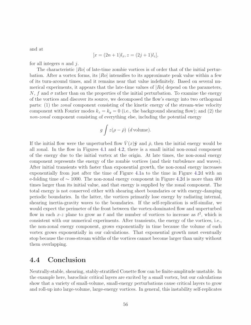
and at[x = (2n+ 1)lx, z = (2j + 1)lz],

for all integers n and j.The characteristic |Ro| of late-time zombie vortices is of order that of the initial pertur-

bation. After a vortex forms, its |Ro| intensifies to its approximate peak value within a fewof its turn-around times, and it remains near that value indefinitely. Based on several nu-merical experiments, it appears that the late-time values of |Ro| depend on the parameters,N , f and σ rather than on the properties of the initial perturbation. To examine the energyof the vortices and discover its source, we decomposed the flow’s energy into two orthogonalparts: (1) the zonal component consisting of the kinetic energy of the stream-wise velocitycomponent with Fourier modes kz = ky = 0 (i.e., the background shearing flow); and (2) thenon-zonal component consisting of everything else, including the potential energy

g

∫z(ρ− ρ) (d volume).

If the initial flow were the unperturbed flow V (x)y and ρ, then the initial energy would beall zonal. In the flow in Figures 4.1 and 4.2, there is a small initial non-zonal componentof the energy due to the initial vortex at the origin. At late times, the non-zonal energycomponent represents the energy of the zombie vortices (and their turbulence and waves).After initial transients with faster than exponential growth, the non-zonal energy increasesexponentially from just after the time of Figure 4.1a to the time in Figure 4.2d with ane-folding time of ∼ 1000. The non-zonal energy component in Figure 4.2d is more than 400times larger than its initial value, and that energy is supplied by the zonal component. Thetotal energy is not conserved either with shearing sheet boundaries or with energy-dampingperiodic boundaries. In the latter, the vortices primarily lose energy by radiating internal,shearing inertia-gravity waves to the boundaries. If the self-replication is self-similar, wewould expect the perimeter of the front between the vortex-dominated flow and unperturbedflow in each x-z plane to grow as t and the number of vortices to increase as t2, which isconsistent with our numerical experiments. After transients, the energy of the vortices, i.e.,the non-zonal energy component, grows exponentially in time because the volume of eachvortex grows exponentially in our calculations. That exponential growth must eventuallystop because the cross-stream widths of the vortices cannot become larger than unity withoutthem overlapping.

4.4 Conclusion

Neutrally-stable, shearing, stably-stratified Couette flow can be finite-amplitude unstable. Inthe example here, baroclinic critical layers are excited by a small vortex, but our calculationsshow that a variety of small-volume, small-energy perturbations cause critical layers to growand roll-up into large-volume, large-energy vortices. In general, this instability self-replicates

56

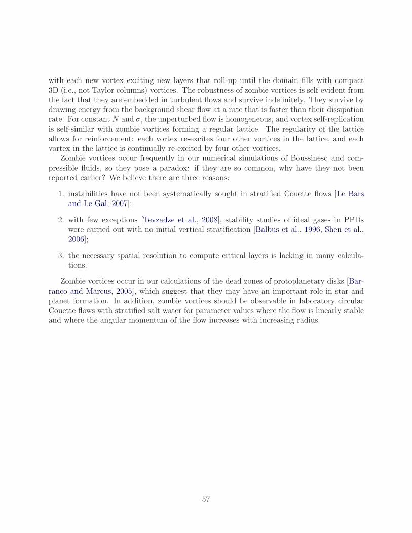
with each new vortex exciting new layers that roll-up until the domain fills with compact3D (i.e., not Taylor columns) vortices. The robustness of zombie vortices is self-evident fromthe fact that they are embedded in turbulent flows and survive indefinitely. They survive bydrawing energy from the background shear flow at a rate that is faster than their dissipationrate. For constant N and σ, the unperturbed flow is homogeneous, and vortex self-replicationis self-similar with zombie vortices forming a regular lattice. The regularity of the latticeallows for reinforcement: each vortex re-excites four other vortices in the lattice, and eachvortex in the lattice is continually re-excited by four other vortices.

Zombie vortices occur frequently in our numerical simulations of Boussinesq and com-pressible fluids, so they pose a paradox: if they are so common, why have they not beenreported earlier? We believe there are three reasons:

1. instabilities have not been systematically sought in stratified Couette flows [Le Barsand Le Gal, 2007];

2. with few exceptions [Tevzadze et al., 2008], stability studies of ideal gases in PPDswere carried out with no initial vertical stratification [Balbus et al., 1996, Shen et al.,2006];

3. the necessary spatial resolution to compute critical layers is lacking in many calcula-tions.

Zombie vortices occur in our calculations of the dead zones of protoplanetary disks [Bar-ranco and Marcus, 2005], which suggest that they may have an important role in star andplanet formation. In addition, zombie vortices should be observable in laboratory circularCouette flows with stratified salt water for parameter values where the flow is linearly stableand where the angular momentum of the flow increases with increasing radius.

57

58

Appendix A

Suction Rate Function qo(x)

As discussed in section 3.3, qo(x) is nearly uniform and negative inside a spherical region ofradius R located at the center of the domain x = 0. Outside the spherical region, qo decaysrapidly. Therefore, the profile of qo in each direction looks like a top–hat function of width2R with smoothed edges.

In a triply periodic domain, the integral of qo(x) over the entire domain must be zero.This is because, integrating (3.7) over the entire domain gives∫

∂u

∂xdx︸ ︷︷ ︸

=0

+

∫∂v

∂ydx︸ ︷︷ ︸

=0

+

∫∂w

∂zdx︸ ︷︷ ︸

=0

=

∫qo(x)dx (A.1)

where each term on the left–hand side is found to be zero using the divergence theorem andperiodicity (the time dependence of q is ignored for simplicity). The integral of qo(x) over thespherical suction region (i.e., sink) is equal to Qo < 0. Therefore, to satisfy the requirementin (A.1), an injection region (i.e., source) must exist in the domain. In another word, this isbecause the sucked flow cannot be supplied through periodic boundaries.

Here we have chosen to evenly spread the source over the entire space outside the sphericalsink. Therefore, the integral of qo(x) over the region outside the spherical suction region is−Qo > 0. Because the volume of a sphere with radius R is much smaller than the volume ofthe entire domain with width D = 20R, the distributed injection qo > 0 (outside the sphere)is much weaker than the localized suction qo < 0 (inside the sphere). As a result, this choiceof source is not expected to significantly affect the flow field. Particularly, we remind thereader that because of the third term on the right–hand side of (3.10), the (small) amount offluid injected into the domain at each point has the same momentum as the local momentumof the flow. Excluding this term would have resulted in injecting fluid with zero velocity intoa point that might have non-zero local velocity, resulting in a fictitious drag. Such drag canbe significant in a strongly rotating flow where velocities are large even far from the sinkbecause of the (background) solid–body rotation.

Note that unlike Davey and Killworth [1989], McDonald [1992] and us, Aiki and Yama-gata [2000, 2004] did not include the equivalent of the ρqv term on the right–hand side of

(3.10) in their shallow–water equations. Therefore, the ρqv term arising from the ∇ · (ρvv)term on the left hand–side of (3.10) is not canceled out in the formulation presented byAiki and Yamagata [2000] (their equation (2.3)). However, these authors did not includethe contribution of the solid–body rotation to the velocity field of the shallow–water equiv-alent of the uncanceled ρqv term, resulting in this term (in the rotating frame) being smallcompared to the Coriolis term. As a result, Aiki and Yamagata [2000] found their results tobe insensitive to the existence of this term, and not significantly different from the resultsreported by Davey and Killworth [1989].

59

60

Bibliography

M. A. Abramowicz, A. Lanza, E. A. Spiegel, and E. Szuszkiewicz. Vortices on accretiondisks. Nature, 356(6364):41–43, 1992.

H. Aiki and T. Yamagata. Successive formation of planetary lenses in an intermediate layer.Geophysical & Astrophysical Fluid Dynamics, 92(1-2):1–29, 2000.

H. Aiki and T. Yamagata. A numerical study on the successive formation of Meddy-likelenses. Journal of Geophysical Research: Oceans, 109, 2004.

L. Armi, D. Hebert, N. Oakey, J. F. Price, P. L. Richardson, H. T. Rossby, and B. Ruddick.The history and decay of a Mediterranean salt lens. Nature, 333(6174):649–651, 1988.

L. Armi, D. Hebert, N. Oakey, J. F. Price, P. L. Richardson, H. T. Rossby, and B. Ruddick.Two years in the life of a Mediterranean salt lens. Journal of Physical Oceanography, 19(3):354–370, 1989.

P. J. Armitage. Dynamics of protoplanetary disks. Annual Review of Astronomy and Astro-physics, 49:195–236, 2011.

O. Aubert, M. Le Bars, P. Le Gal, and P. S. Marcus. The universal aspect ratio of vorticesin rotating stratified flows: experiments and observations. Journal of Fluid Mechanics,706:34, 2012.

S. A. Balbus and J. F. Hawley. Instability, turbulence, and enhanced transport in accretiondisks. Reviews of Modern Physics, 70(1), 1998.

S. A. Balbus, J. F. Hawley, and J. M. Stone. Nonlinear stability, hydrodynamical turbulence,and transport in disks. The Astrophysical Journal, 467, 1996.

V. Barcilon and J. Pedlosky. On the steady motions produced by a stable stratification in arapidly rotating fluid. Journal of Fluid Mechanics, 29:673–690, 1967.

P. Barge and J. Sommeria. Did planet formation begin inside persistent gaseous vortices.Astronomy and Astrophysics, 295(1):L1–L4, 1995.

J. A. Barranco and P. S. Marcus. Three-dimensional vortices in stratified protoplanetarydisks. Astrophysical Journal, 623(2):1157–1170, 2005.

J. A. Barranco and P. S. Marcus. A 3D spectral anelastic hydrodynamic code for shearing,stratified flows. Journal of Computational Physics, 219(1):21–46, 2006.

P. Billant and J-M Chomaz. Self-similarity of strongly stratified inviscid flows. Physics ofFluids, 13(6):1645–1651, 2001.

N. Boulanger, P. Meunier, and S. Le Dizes. Structure of a stratified tilted vortex. Journalof Fluid Mechanics, 583(1):443–458, 2007.

A. Bracco, P. H. Chavanis, A. Provenzale, and E. A. Spiegel. Particle aggregation in aturbulent Keplerian flow. Physics of Fluids, 11:2280, 1999.

J. W. M. Bush and A. W. Woods. Vortex generation by line plumes in a rotating stratifiedfluid. Journal of Fluid Mechanics, 388:289–313, 1999.

X. Carton. Hydrodynamical modeling of oceanic vortices. Surveys in Geophysics, 22(3):79–263, 2001.

C. Cenedese and P. F. Linden. Cyclone and anticyclone formation in a rotating stratifiedfluid over a sloping bottom. Journal of Fluid Mechanics, 381:199–223, 1999.

J. G. Charney. Geostrophic turbulence. Journal of the Atmospheric Sciences, 28:1087–1095,1971.

J. Y. K. Cho and L. M. Polvani. The emergence of jets and vortices in freely evolving,shallow–water turbulence on a sphere. Physics of Fluids, 8(6):1531–1552, 1996a.

J. Y-K. Cho and L. M. Polvani. The morphogenesis of bands and zonal winds in the atmo-spheres on the giant outer planets. Science, pages 335–336, 1996b.

S. B. Dalziel, G. O. Hughes, and B. R. Sutherland. Whole-field density measurements bysynthetic schlieren. Experiments in Fluids, 28(4):322–335, 2000.

M. K. Davey and P. D. Killworth. Flows produced by discrete sources of buoyancy. Journalof Physical Oceanography, 19:1279–1290, 1989.

I. de Pater, M. H. Wong, P. S. Marcus, S. Luszcz-Cook, M. Adamkovics, A. Conrad, X. Asay-Davis, and C. Go. Persistent rings in and around Jupiter’s anticyclones–observations andtheory. Icarus, 210(2):742–762, 2010.

P. G. Drazin and W. H. Reid. Hydrodynamic stability. Cambridge University Press, 2004.

D. G. Dritschel, M. D. Juarez, and M. H. P. Ambaum. The three-dimensional vortical natureof atmospheric and oceanic turbulent flows. Physics of Fluids, 11(6):1512–1520, 1999.

L. N Fletcher et al. Thermal structure and composition of Jupiters Great Red Spot fromhigh-resolution thermal imaging. Icarus, 208(1):306–328, 2010.

61

P. R. Gent and J. C. McWilliams. The instability of barotropic circular vortices. Geophysicaland Astrophysical Fluid Dynamics, 35:209–233, 1986.

M. Ghil, M. D. Chekroun, and E. Simonnet. Climate dynamics and fluid mechanics: Naturalvariability and related uncertainties. Physica D: Nonlinear Phenomena, 237(14):2111–2126, 2008.

A. E. Gill. Homogeneous intrusions in a rotating stratified fluid. Journal of Fluid Mechanics,103:275–295, 1981.

C. Y. Go, I. de Pater, M. Wong, S. Lockwood, P. S. Marcus, X. Asay-Davis, and S. Shetty.Evolution of the Oval BA during 2004–2005. In Bulletin of the American AstronomicalSociety, volume 38, page 495, 2006.

D. A. Godfrey. A hexagonal feature around Saturn’s North Pole. Icarus, 76(2):335–356,1988.

P. Goldreich and D. Lynden-Bell. Ii. spiral arms as sheared gravitational instabilities.Monthly Notices of the Royal Astronomical Society, 130:125, 1965.

L. P. Graves, J. C. McWilliams, and M. T. Montgomery. Vortex evolution due to straining:a mechanism for dominance of strong, interior anticyclones. Geophysical & AstrophysicalFluid Dynamics, 100(3):151–183, June 2006.

H. P. Greenspan. The theory of rotating fluids. Cambridge University Press, 1990.

R. W. Griffiths and P. F. Linden. The stability of vortices in a rotating, stratified fluid.Journal of Fluid Mechanics, 105:283–316, 1981.

G. J. Hakim, C. Snyder, and D. J. Muraki. A new surface model for cyclone–anticycloneasymmetry. Journal of the Atmospheric Sciences, 59(16):2405–2420, 2002.

P. Hassanzadeh and P. S. Marcus. 3d baroclinic vortices in rotating stratified shear: from anorange great red spot to planet formation. In Bulletin of the American Physical Society,volume 57. APS, 2012.

P. Hassanzadeh, P. S. Marcus, and P. Le Gal. The universal aspect ratio of vortices inrotating stratified flows: theory and simulation. Journal of Fluid Mechanics, 706:46, 2012.

P. Hassanzadeh, O. Aubert, P. S. Marcus, M. Le Bars, and P. Le Gal. Three–dimensionalcyclones produced by localised suction in rotating stratified flows: a numerical and exper-imental study. to be submitted to the Journal of Fluid Mechanics, 2013.

H. J. Head. The use of miniature four-electrode conductivity probes for high-resolution mea-surements of turbulent density or temperature variations in salt-stratified water flows. PhDthesis, University of California, San Diego, 1983.

62

K. Hedstrom and L. Armi. An experimental-study of homogeneous lenses in a stratifiedrotating fluid. Journal of Fluid Mechanics, 191:535–556, 1988.

A. J. Hines, A.and Willmott. Unsteady abyssal circulation driven by a discrete buoyancysource in a continuously stratified ocean. Journal of Physical Oceanography, 27(7):1349–1370, 1997.

R. Hooke. A spot in one of the belts of Jupiter. Philosophical Transactions, 1, 1665.

T. Humphreys and P. S. Marcus. Vortex street dynamics: The selection mechanism forthe areas and locations of Jupiter’s vortices. Journal of the Atmospheric Sciences, 64(4):1318–1333, 2007.

A. P. Ingersoll. Atmospheric dynamics of the outer planets. Science, 248(4953):308–315,1990.

A. P. Ingersoll and P. G. Cuong. Numerical model of long–lived Jovian vortices. Journal ofthe Atmospheric Sciences, 38(10):2067–2076, 1981.

A. Jenkins. An elementary treatment of the reverse sprinkler. American Journal of Physics,72(10):1276–1283, 2004.

H. Ji, M. Burin, E. Schartman, and J. Goodman. Hydrodynamic turbulence cannot transportangular momentum effectively in astrophysical disks. Nature, 444(7117):343–346, 2006.

B. Khouider, A. J. Majda, and S. N. Stechmann. Climate science in the tropics: waves,vortices and PDEs. Nonlinearity, 26(1):R1, 2013.

H. Klahr and P. Bodenheimer. Formation of giant planets by concurrent accretion of solidsand gas inside an anticyclonic vortex. The Astrophysical Journal, 639(1):432, 2006.

P. Klein and G. Lapeyre. The oceanic vertical pump induced by mesoscale and submesoscaleturbulence. Annual Review of Marine Science, 1:351–375, 2009.

I. Koszalka, A. Bracco, J. C. McWilliams, and A. Provenzale. Dynamics of wind–forcedcoherent anticyclones in the open ocean. Journal of Geophysical Research, 114, 2009.

P. K. Kundu and I. M. Cohen. Fluid Mechanics. Academic Press, 2010.

M. Le Bars and P. Le Gal. Experimental analysis of the stratorotational instability in acylindrical Couette flow. Physical Review Letters, 99(6), 2007.

P. F. Linden, B. M. Boubnov, and S. B. Dalziel. Source–sink turbulence in a rotatingstratified fluid. Journal of Fluid Mechanics, 298(1):81–112, 1995.

J. J. Lissauer. Planet formation. Annual Review of Astronomy and Astrophysics, 31:129–174,1993.

63

R. V. E. Lovelace, H. Li, S. A. Colgate, and A. F. Nelson. Rossby wave instability ofKeplerian accretion disks. The Astrophysical Journal, 513(2), 1999.

W. Lyra and M-M Mac Low. Rossby wave instability at Dead Zone boundaries in three–dimensional resistive magnetohydrodynamical global models of protoplanetary disks. TheAstrophysical Journal, 756(1):62, 2012.

M-M Mac Low and A. P. Ingersoll. Merging of vortices in the atmosphere of Jupiter: Ananalysis of Voyager images. Icarus, 65(2):353–369, 1986.

P. S. Marcus. Numerical-simulation of Jupiter’s Great Red Spot. Nature, 331(6158):693–696,1988.

P. S. Marcus. Vortex dynamics in a shearing zonal flow. Journal of Fluid Mechanics, 215:393–430, 1990.

P. S. Marcus. Jupiter’s Great Red Spot and other vortices. Annual Review of Astronomyand Astrophysics, 31:523–573, 1993.

P. S. Marcus. Prediction of a global climate change on Jupiter. Nature, 428(6985):828–831,2004.

P. S. Marcus and P. Hassanzadeh. 3D vortices in stratified, rotating flows-secondary circula-tions and changes in aspect radio due to dissipation. In Bulletin of the American PhysicalSociety, volume 56. APS, 2011.

P. S. Marcus and W. H. Press. On Green’s functions for small disturbances of plane Couetteflow. Journal of Fluid Mechanics, 79(03):525–534, 1977.

P. S. Marcus, X. S. Asay-Davis, M. H. Wong, and I. de Pater. Jupiters Red Oval BA:Dynamics, color, and relationship to Jovian climate change. Journal of Heat Transfer,135, 2013a.

P. S. Marcus, S. Pei, C-H Jiang, and P. Hassanzadeh. Self–replicating three–dimensionalvortices in neutrally–stable stratified rotating shear flows. submitted to the Physical ReviewLetters, 2013b.

N. R. McDonald. Flows caused by mass forcing in a stratified ocean. Deep Sea Research A,39(10):1767–1790, 1992.

M. E. McIntyre. On the antarctic ozone hole. Journal of Atmospheric and TerrestrialPhysics, 51(1):29–43, 1989.

M. E. McIntyre. The stratospheric polar vortex and sub-vortex: Fluid dynamics and midlat-itude ozone loss. Philosophical Transactions of the Royal Society of London A, 352(1699):227–240, 1995.

64

C. F. McKee and E. C. Ostriker. Theory of star formation. Annual Review of Astronomyand Astrophysics, 45(1):565–687, 2007.

J. C. McWilliams. Submesoscale, coherent vortices in the ocean. Reviews of Geophysics, 23(2):165–182, 1985.

J. C. McWilliams. Vortex generation through balanced adjustment. Journal of PhysicalOceanography, 18(8):1178–1192, 1988.

J. C. McWilliams, J. B. Weiss, and I. Yavneh. Anisotropy and coherent vortex structures inplanetary turbulence. Science, 264(5157):410–413, 1994.

J. C. McWilliams, J. B. Weiss, and I. Yavneh. The vortices of homogeneous geostrophicturbulence. Journal of Fluid Mechanics, 401:1–26, 1999.

F. Moisy, C. Morize, M. Rabaud, and J. Sommeria. Decay laws, anisotropy and cyclone–anticyclone asymmetry in decaying rotating turbulence. Journal of Fluid Mechanics, 666:5–35, October 2010.

R. Morales-Juberıas and T. E. Dowling. Jupiters Great Red Spot: Fine–scale matches ofmodel vorticity patterns to prevailing cloud patterns. Icarus, 2013.

Y. Morel and J. McWilliams. Evolution of isolated interior vortices in the ocean. Journal ofPhysical Oceanography, 27(5):727–748, 1997.

D. Nof. On the β-induced movement of isolated baroclinic eddies. Journal of PhysicalOceanography, 11(12):1662–1672, 1981.

D. B. Olson. Rings in the ocean. Annual Review of Earth and Planetary Sciences, 19:283,1991.

M. S. Paoletti, D. P. M. van Gils, B. Dubrulle, C. Sun, D. Lohse, and D. P. Lathrop. Angularmomentum transport and turbulence in laboratory models of Keplerian flows. Astronomy& Astrophysics, 547, 2012.

J. Pedlosky. Geophysical fluid dynamics. Springer–Verlag, 1990.

G. Perret, A. Stegner, M. Farge, and T. Pichon. Cyclone–anticyclone asymmetry of large–scale wakes in the laboratory. Physics of Fluids, 18, 2006.

G. Perret, T. Dubos, and A. Stegner. How large–scale and cyclogeostrophic barotropicinstabilities favor the formation of anticyclonic vortices in the ocean. Journal of PhysicalOceanography, 41(2):303–328, 2011.

L. M. Polvani, J. C. McWilliams, M. A. Spall, and R. Ford. The coherent structures ofshallow–water turbulence: Deformation–radius effects, cyclone/anticyclone asymmetryand gravity–wave generation. Chaos: An Interdisciplinary Journal of Nonlinear Science,4(2):177–186, 1994.

65

O. Praud, J. Sommeria, and A. M. Fincham. Decaying grid turbulence in a rotating stratifiedfluid. Journal of Fluid Mechanics, 547:389–412, 2006.

Lord Rayleigh. On the dynamics of revolving fluids. Proceedings of the Royal Society ofLondon. Series A, 93(648):148–154, 1917.

J. N. Reinaud, D. G. Dritschel, and C. R. Koudella. The shape of vortices in quasi-geostrophicturbulence. Journal of Fluid Mechanics, 474:175–192, 2003.

C-G Rossby. A mechanism for the release of potential energy in the atmosphere. Journal ofAtmospheric Sciences, 6:164–180, 1949.

G. Roullet and P. Klein. Cyclone–anticyclone asymmetry in geophysical turbulence. PhysicalReview Letters, 104(21):28–31, 2010.

C. Salyk, A. P. Ingersoll, J. Lorre, A. Vasavada, and A. D. Del Genio. Interaction betweeneddies and mean flow in Jupiter’s atmosphere: Analysis of Cassini imaging data. Icarus,185(2):430–442, 2006.

A. Sanchez-Lavega, R. Hueso, S. Perez-Hoyos, and J. F. Rojas. A strong vortex in Saturn’sSouth Pole. Icarus, 184(2):524–531, 2006.

P. Sangra et al. The Canary eddy corridor: A major pathway for long–lived eddies in thesubtropical North Atlantic. Deep–Sea Research I, 56(12):2100–2114, 2009.

K. M. Sayanagi, P. Morales-Juberias, and A. P. Ingersoll. Saturn’s Northern HemisphereRibbon: Simulations and comparison with the meandering Gulf Stream. Journal of theAtmospheric Sciences, 67(8):2658–2678, 2010.

Y. Shen, J. M. Stone, and T. A. Gardiner. Three-dimensional compressible hydrodynamicsimulations of vortices in disks. The Astrophysical Journal, 653(1), 2006.

S. Shetty and P. S. Marcus. Changes in Jupiter’s Great Red Spot (1979-2006) and Oval BA(2000-2006). Icarus, 210(1):182–2018, 2010.

S. Shetty, X. S. Asay-Davis, and P. S. Marcus. On the interaction of Jupiter’s Great RedSpot and zonal jet streams. Journal of the Atmospheric Sciences, 64, 2007.

A. Siegel, J. B. Weiss, J. Toomre, J. C. McWilliams, P. S. Berloff, and I. Yavneh. Eddies andvortices in ocean basin dynamics. Geophysical Research Letters, 28(16):3183–3186, 2001.

B. A. Smith et al. Voyager 2 at Neptune: Imaging science results. Science, 246(4936), 1989.

W. D. Smyth and J. C. McWilliams. Instability of an axisymmetric vortex in a stablystratified, rotating environment. Theoretical and Computational Fluid Dynamics, 11(3):305–322, 1998.

66

J. Sommeria, S. D. Meyers, and H. L. Swinney. Laboratory simulation of Jupiters great redspot. Nature, 331(6158):689–693, 1988.

A. Stegner and D. G. Dritschel. A Numerical Investigation of the Stability of Isolated ShallowWater Vortices. Journal of Physical Oceanography, 30(10):2562–2573, October 2000.

G. A. Stuart, M. A. Sundermeyer, and D. Hebert. On the geostrophic adjustment of anisolated lens: Dependence on burger number and initial geometry. Journal of PhysicalOceanography, 41(4):725–741, 2011.

A. G. Tevzadze, G. D. Chagelishvili, and J. P. Zahn. Hydrodynamic stability and modecoupling in Keplerian flows: local strato-rotational analysis. Astronomy and Astrophysics,478(1):9–15, 2008.

G. K. Vallis. Atmospheric and Oceanic Fluid Dynamics. Cambridge University Press, 2006.

G. J. F. van Heijst and H. J. H. Clercx. Laboratory Modeling of Geophysical Vortices.Annual Review of Fluid Mechanics, 41:143–164, 2009.

G. J. F. van Heijst and R. C. Kloosterziel. Tripolar vortices in a rotating fluid. Nature, 338(6216):569–571, 1989.

A. R. Vasavada and A. P. Showman. Jovian atmospheric dynamics: An update after Galileoand Cassini. Reports on Progress in Physics, 68(8):1935–1996, 2005.

H. von Zeipel. The radiative equilibrium of a rotating system of gaseous masses. MonthlyNotices of the Royal Astronomical Society, 84:665–683, 1924.

D. W. Waugh and L. M. Polvani. Stratospheric polar vortices. The Stratosphere: Dynamics,Transport, and Chemistry, Geophysics Monograph Series, 190:43–57, 2010.

M. H. Wong, I. de Pater, X. Asay-Davis, P. S. Marcus, and C. Y. Go. Vertical structure ofJupiters Oval BA before and after it reddened: What changed? Icarus, 215(1):211–225,2011.

W. Zenk and L. Armi. The complex spreading pattern of Mediterranean water off thePortuguese continental slope. Deep–Sea Research, 37(12):1805–1823, 1990.

67