Embed Size (px)
Citation preview

1
The Exchange Rate Sensitivity of Foreign Trade: Evidence from Malawi
Ronald Mangani University of Malawi, Chancellor College, Department of Economics
Email: [email protected]
Abstract
This study examined the effects of the exchange rate on foreign trade in Malawi. Separate export
value and import value models were estimated using the single equation error correction modelling
framework proposed by Pesaran et al. (2001). Apart from the real effective exchange rate, the aggregate
GDP of Malawi’s key trading partners was included in the export value function, while Malawi’s own
GDP was allowed to explain the value of imports. The findings documented in this paper show that
foreign trade in Malawi was not responsive to the real effective exchange rate, both in the long-run and in
the short-run. Thus, there was no compelling support for either the Marshall-Lerner condition or the J-
curve effect. These results suggest that exchange rate policy should focus more on other national
considerations (such as influencing imported inflation) than the trade balance. They particularly imply
that welfare maximisation may be attained through exchange rate policy at no opportunity cost of
deterioration in the trade balance. They also suggest that Malawi’s persistently precarious foreign reserve
position is a result more of the unavailability of adequate reserves than the effect of currency
overvaluation on trade.

1
The Exchange Rate Sensitivity of Foreign Trade: Evidence from Malawi
1. Introduction
This study examined the effects of the real effective exchange rate on the aggregate foreign trade
flows in Malawi, in order to inform the formulation of exchange rate policy. Exchange rate policy
continues to attract significant interest among economists, because the exchange rate has key theoretical
bearings on many macroeconomic variables including the balance of payments, domestic prices and
international reserves. Within the context of Malawi, the combination of a low export base and high
dependence on imports paused a challenge in terms of preserving the domestic and external values of the
local currency (the Malawi kwacha). While the established economic theory posits that an overvalued
domestic currency relative to foreign exchange worsens the country’s trade balance and foreign reserve
position (Marshall, 1923; Lerner, 1944), it is also the case that domestic currency depreciation can be
inflationary, especially in highly import-based economies. The latter effect can be described through yet
another entrenched theory, the purchasing power parity (PPP) hypothesis seminally popularised by Cassel
(1918). As such authorities typically face a crucial dilemma in the exchange rate policy objective
function, especially when their capacity to defend the domestic currency is compromised by foreign
reserve limitations.
Intuition, observation and analytical work strongly suggested that the exchange rate was a key
determinant of domestic prices in Malawi. Immediately upon currency flotation in 1994, the 62.0 percent
resultant devaluation of the Malawi kwacha accounted for the most inflationary period in Malawi: annual
inflation reached the pick of 60.6 percent in 1995. Mangani (2011) documents evidence that the exchange
rate was the single most importance variable in explaining price dynamics in Malawi, and that its effects
were transmitted directly rather than through the exchange rate channel of the monetary policy
transmission mechanism. Additional evidence in this regard is provided by Ngalawa (2009). On the other
hand, although some commentators posit that the welfare implications of currency devaluation outweigh
its benefits in Malawi, credible quantitative evidence on the effects of the exchange rate on the country’s
balance of payments in general - and the trade balance in particular – remained wanting. This paper
contributes to this debate by establishing that the exchange rate has no significant effects on Malawi’s
trade flows.
The paper proceeds as follows. Section 2 discusses Malawi’s exchange rate policy developments
in order to locate the ensuing analysis in the national context. The methodologies adopted in the study are
presented in Section 3, while Section 4 presents the findings. A conclusion in made in Section 5.

2
2. Exchange rate policy in Malawi1
Malawi is a heavily import-dependent economy and exchange rate policy is as crucial as
conventional monetary policy. Thus, in addition to the control of demand-pull inflation resulting from
swelling money supply, the central bank has to deal with cost-push inflation largely arising from domestic
currency devaluation and exogenous shocks. Malawi’s foreign reserve position is quite precarious due to
excessive dependence on two key but wobbly sources: tobacco exports and development assistance.
Failures in rain-fed agriculture and donor inflows induce sometimes unsustainable interventionist
activities from the authorities, or directly impact on domestic prices when authorities succumb to the
resultant foreign exchange shortages by invoking currency devaluation to address external imbalances.
Moreover, the country’s land-lockedness and heavy reliance on imported oil for energy have great
potential to induce imported inflation and to undermine monetary policy. The exchange rate clearly
emerges as the nominal anchor of stabilisation in Malawi.
Various exchange rate regimes have been pursued in Malawi during its history. The Malawi
kwacha (MK) was pegged to the British pound sterling (GBP) at one-to-one from 1964 to 1967, and at
MK2.00 per GBP between 1967 and 1973. Following the collapse of the Bretton Woods’ fixed exchange
rate system, the kwacha was pegged to a trade-weighted average of the pound sterling and the United
States dollar (US$) from November 1973 to June 1975, and to the Special Drawing Rights (SDR) at
almost one-to-one between July 1975 and January 1984. In response to an expansion in Malawi’s trade
volume and trading partners, the kwacha was subsequently pegged to a trade-weighted basket of seven
currencies (US$, GBP, German deutschemark, South African rand, French franc, Japanese yen, and
Dutch guilder) between 1984 and 1994. This period was characterised by frequent devaluations
implemented in the context of the structural adjustment programmes supported by the International
Monetary Fund (IMF), in an attempt to improve the country’s export competitiveness and balance of
payments position. Five devaluations in the magnitudes of 7 percent to 22 percent against the US$ were
effected between February 1986, and August 1992. In February 1994, the kwacha was purportedly
floated, and an interbank foreign exchange market was introduced to determine the exchange rate. The
current account was liberalised consequently, although the capital account was not liberalised and some
exchange controls (such as limitations on foreign exchange allowances for travel, remittances,
repatriations and importation of consumer goods) remained in place. The immediate effect of the flotation
was a 62.0 percent depreciation of the domestic currency between February and December 1994, from
MK5.92 to MK15.58 per US$.
1 Most of this account is derived from Mangani (2011).
3
Given the limited number of players on the market which constrained the foreign exchange
bidding process, the government adopted a managed floating system in 1995. This system permitted the
authorities to intervene in order to artificially influence the exchange rate through sales and purchases of
foreign currency, hence managing it within a narrow band. However, the band was removed later in 1998
in favour of a free float, only to be reinstated with a very narrow flexibility range in mid 2006.
Although maintaining stability of the exchange rate is a prime objective of the Government, it is
clear that the attainment of this objective is quite a challenge. Due to a multiplicity of factors (such as
excessive dependence on imported raw materials, intermediate inputs and final consumer goods; currency
over-valuation; a narrow export base), Malawi’s trade balance and balance of payments positions are
almost perpetually negative, and have been worsening over time (Tables 1 and 2). Thus, the authorities’
concerted yearning to prevent adverse fluctuations in the exchange rate exerts a lot of pressure on
foreign reserves and the external value of the kwacha, because it reflects a subsidisation of imports.
Table 1 – External trade position (US$ million) 2002 2003 2004 2005 2006 2007* 2008* 2009 2010*
Total imports 699.6 787.0 932.2 1183.7 1268.5 1436.4 1654.5 1574.674 2325.807
Total Exports 409.6 530.5 483.1 503.7 709.1 920.4 1036.6 1118.117 1062.909
Trade balance -290.0 -256.5 -449.1 -680.1 -559.4 -516.0 -617.9 -456.556 -1262.9
Source: Government of Malawi, Annual Economic Report, various. *Estimates
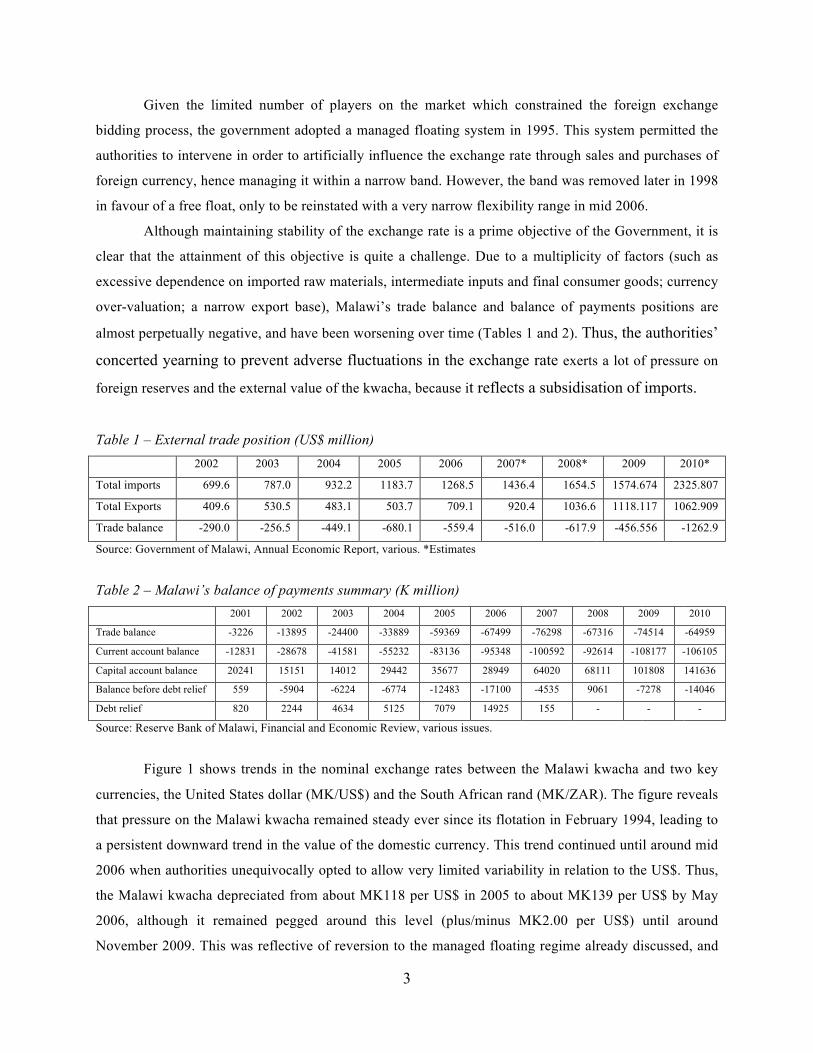
Table 2 – Malawi’s balance of payments summary (K million) 2001 2002 2003 2004 2005 2006 2007 2008 2009 2010
Trade balance -3226 -13895 -24400 -33889 -59369 -67499 -76298 -67316 -74514 -64959
Current account balance -12831 -28678 -41581 -55232 -83136 -95348 -100592 -92614 -108177 -106105
Capital account balance 20241 15151 14012 29442 35677 28949 64020 68111 101808 141636
Balance before debt relief 559 -5904 -6224 -6774 -12483 -17100 -4535 9061 -7278 -14046
Debt relief 820 2244 4634 5125 7079 14925 155 - - -
Source: Reserve Bank of Malawi, Financial and Economic Review, various issues.
Figure 1 shows trends in the nominal exchange rates between the Malawi kwacha and two key
currencies, the United States dollar (MK/US$) and the South African rand (MK/ZAR). The figure reveals
that pressure on the Malawi kwacha remained steady ever since its flotation in February 1994, leading to
a persistent downward trend in the value of the domestic currency. This trend continued until around mid
2006 when authorities unequivocally opted to allow very limited variability in relation to the US$. Thus,
the Malawi kwacha depreciated from about MK118 per US$ in 2005 to about MK139 per US$ by May
2006, although it remained pegged around this level (plus/minus MK2.00 per US$) until around
November 2009. This was reflective of reversion to the managed floating regime already discussed, and

4
was costly on the limited foreign reserves available to the country. The fact that the rate on the parallel
market was usually significantly above the official rate during this period was a telling sign of domestic
currency overvaluation2. Thus, at US$209.5 million in July 2009, total gross official reserves3 were only
equivalent to 1.6 months of imports (Reserve Bank of Malawi, 2009). This represented a marginal
improvement to the level of 1.1 months of imports experienced in January 2009, and 1.3 months in
September 2008, all of which were significantly lower than the 2.5 months recorded in December 2005.
Gross official reserves were estimated at US$302 million or 2.33 months of imports in November
2010,but increased to the equivalent of 3.11 months in January 2011 on account of increased donor
inflows. This increase followed a positive review of the Extended Credit Facility by the IMF in December
2010 (Malawi Savings Bank, 2011).
Figure 1 – Trends in Malawi kwacha exchange rates
Data source: Reserve Bank of Malawi Database
As at 13 May 2011, gross foreign exchange reserves were at $350 million or the equivalent of
2.71 months of imports. This compared favorably with the situation on the same date in 2010, when the
reserves stood at $327 million or 2.54 months of imports4. However, compared with 2010 when foreign
exchange earnings from tobacco stood at $150.6 million by end May, the 2011 tobacco earnings had
declined by 78.8 percent to only $31.9 million as at May 2011. Low tobacco proceeds, high import
2 The CABS Group, March 2009 CABS Review: Aide Memoir. 3 Estimate for the entire Banking System, which includes Gross Official Reserves, Foreign Currency Denominated Accounts (FCDAs) and authorized dealer bank’s (ADB’s) own foreign exchange positions. 4 Malawi Savings Bank Financial and Economic Report, various.
0.00
20.00
40.00
60.00
80.00
100.00
120.00
140.00
160.00
Jan-‐90
Jan-‐91
Jan-‐92
Jan-‐93
Jan-‐94
Jan-‐95
Jan-‐96
Jan-‐97
Jan-‐98
Jan-‐99
Jan-‐00
Jan-‐01
Jan-‐02
Jan-‐03
Jan-‐04
Jan-‐05
Jan-‐06
Jan-‐07
Jan-‐08
Jan-‐09
MK pe
r unit o
f foreign currency
MK/US$
MK/ZAR

5
costs for petroleum products and fertilizers posed challenges on the foreign reserve position. It
was officially reported that only about one half of the foreign exchange requirements of
importers were backed by export proceeds in 2010 (Government of Malawi, 2011). Since 2009,
foreign exchange shortages remained a major factor in stifling industrial growth through fuel
shortages and inability to import inputs, and the IMF5 projected that Malawi’s economic growth
would continue to slow down as a result of this, from 8.9 percent in 2009 and 6.7 percent in 2010
to 6.1 percent and 5.9 percent in 2011 and 2012, respectively. Responding to this persistent pressure
on foreign exchange reserves, the Malawi kwacha weakened and was selling at K147.4 against the United
States dollar at the close of December 2009. By end January 2010, the kwacha was trading at around
K151.5 per U.S. dollar, and remained around that level throughout 2010 and the first half of 2011. A
devaluation of 10 percent was implemented in August 2011 in reaction to the external imbalances.
Given the country’s narrow and vulnerable export base, it is difficult to imagine that, in the short-
to medium-term, a stable market-determined exchange rate regime could be operated without balance of
payments support and other forms of assistance from donors. Yet at the same time, limited flexibility in
the exchange rate tended to create persistent external imbalances. Although there was a strong narrative
regarding the adverse effects of the country’s foreign exchange policies on the trade balance, these effects
had not yet been quantified.
3. Theoretical Framework and the Literature
The conventional wisdom that domestic currency devaluation improves the trade balance is
rooted in a static and partial equilibrium approach to the balance of payments, called the elasticity
approach. This approach is evolutionally formalised in the so-called BRM model due to Bickerdike
(1920), Robinson (1947) and Metzeler (1948), which provides a sufficient condition (the BRM condition)
for trade balance improvement. In particular, domestic currency devaluation makes domestic goods
attractive on the foreign market (hence boosting exports) and foreign goods expensive on the domestic
market (hence restricting imports), both of which effects lead to an improvement in the domestic
country’s trade balance. A particularly stylised form of the BRM condition, popularly called the Marshall-
Lerner condition (Marshall, 1923; Lerner, 1944; hereafter the ML condition), states that for a positive
effect of devaluation on the trade balance to occur, the sum of the exchange rate elasticities of exports and
imports must exceed unity in absolute value terms. When the ML condition holds, the exchange market is
implicitly stable since there will be excess foreign exchange when the exchange rate is above the
5 IMF, World Economic Outlook Report 2011.
6
equilibrium, and vice versa. As such, the ML condition is a long-run (equilibrium) condition empirically
investigated through the exchange rate sensitivity of the imports and exports in level variables.
It is now increasingly recognised that the effects of devaluation on the trade balance occur with a
time lag. As first observed by Magee (1973) as well as Junz and Rhomberg (1973), imports and exports
adjust to changes with time lags which may take such forms as decision lag, recognition lag, production
lag, replacement lag and delivery lag. Importantly, it is argued by some researchers that the trade balance
actually deteriorates in the short-run in response to devaluation, but improves over time towards the ML
condition. Hsing (1999) argues that the degree of foreign and domestic producer’s price pass-through to
consumers and the scale of supply and demand elasticities of exports and imports determine the value of
the exchange rate effect, and these tend to improve with time. This suggests that there is a short-run
discrepancy which is corrected through an adjustment process in each period as the economy progresses
to equilibrium (Bahmani-Oskooee and Ratha, 2004). The time path of the effects of devaluation on the
trade balance, therefore, traces the so-called J-curve. Empirically, most work on the J-curve effect has
benefitted from the application of cointegration and error correction techniques, building on the work of
Bahmani-Oskooee (1985).
Models explaining both the ML condition and the J-curve effects typically express the trade
balance as a function of domestic income, foreign income and the exchange rate, where the income
variables are control variables while interest is on calibrating the exchange rate effects. Exports and
imports may also be individually modelled in a similar manner. Mixed empirical evidence exists on the
exchange rate sensitivity of the trade balance. A sample of the mixed evidence on the ML condition is in
Summary (1989), Nadenichek (2000), Narayana and Narayana (2005), Bahmani-Oskooee and Goswami
(2004), and Arize (2001). Equally mixed evidence on J-curve effects has also been documented for many
countries, including Japan (Gupta-Kapoor and Ramakrishnan, 1999), Croatia (Tihomir, 2004), the USA
(Bahmani-Oskooee and Ratha, 2008; Koch and Rosensweig, 1990;), Taiwan (Hsing, 2003), some
ASEAN countries (Onafowora, 2003), as well as a selection of 13 developing countries from Asia, Latin
America and Europe (Bahmani-Oskooee, 1991). Kamoto (2006) documents evidence of J-curve effects
for South Africa.
Using a vector error correction modeling framework, Kamoto (2006) was unable to find a
statistically significant J-curve effect in Malawi, although he was able to detect evidence of the long-run
effect. Very little else has been documented on this subject using data from Malawi where debate on the
macroeconomic effects of exchange rate policy is rife. The present study applies a recently proposed error
correction modeling framework to add to the very limited evidence from Malawi.
7
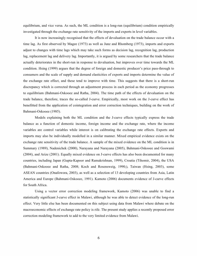
4. Methodology
4.1 The models
Building on Bahmani-Oskooee and Goswami (2004) and following Bahmani-Oskooee and Ratha
(2008), the following log-linear export value and import value models can be specified:
*
0 1 2 1ln ln lnt t t tX Y Eα α α µ= + + + (1)
0 1 2 2ln ln lnt t t tM Y Eβ β β µ= + + + (2) where t denotes time, !! and !! are the values of Malawi’s exports and imports, while 1µ and
2µ are white noise error terms. In addition to the real effective exchange rate ( tE ), exports could also
depend on the income level of Malawi’s trading partners ( *tY ), while imports could depend on the level of
Malawi’s income ( tY ). All the variables are expressed in natural logarithmic levels, while iα and jβ (
, 0,1,2i j = ) are parameters to be estimated. It is expected that both 1α and 1β should be positive,
indicating that the value of exports increases with *tY while that of imports increases with tY , ceteris
paribus. Since an increase in the real effective exchange rate as reported in the International Financial
Statistics (IFS) of the IMF represents an appreciation of the domestic currency relative to foreign
currency, it is expected that 2 0α < and that 2 0β > . This is premised on the theoretical proposition that
a higher external value of the kwacha makes foreign goods price-attractive to Malawians, and makes
Malawian products unattractive to foreigners.
Advances in time series econometrics suggest that in the estimation of long-run relationships such
as equations (1) and (2), the short-run dynamics must be incorporated in order to account for the
adjustment path towards the long-run. Therefore, the study estimated the following error correction
models which do not require explicit unit roots testing, in the spirit of Pesaran et al. (2001):
* *
1 1 2 1 3 1 11 1 1
ln ln ln ln ln ln lnm m m
t i it i t i i t i i t i t t t ti i i
X aQ X Y E X Y Eρ δ π φ φ φ ε− − − − − −= = =
Δ = + Δ + + + + + +∑ ∑ ∑ (3)
1 1 2 1 3 1 21 1 1
ln ln ln ln ln ln lnn n n
t i it k t k k t k k t k t t t tk k k
M bQ M Y E M Y Eγ λ η ϕ ϕ ϕ ε− − − − − −= = =
Δ = + Δ + + + + + +∑ ∑ ∑
(4) where Δ is the first difference operator and itQ has been added to capture the inclusion of
intercept terms, trend terms, dummy variables, and such other deterministic terms that may be suggested

8
by the data generating processes. 1tε and 2tε are white noise error terms. All other variables are as
defined for equations (1) and (2), and parameters to be estimated have obvious notation. In these error
correction specifications, cointegration is confirmed in the export value function if the iφ coefficients are
jointly significant. Similarly, the import value function is cointegrated if the kϕ coefficients are jointly
significant. Thus, the cointegartion tests were based on the null hypotheses of 1 2 3 0φ φ φ= = = and
1 2 3 0ϕ ϕ ϕ= = = in the environment of standard Wald tests for linear restrictions. Pesaran et al. (2001)
provide the upper and lower bound critical values for resolving this hypothesis, based on the standard F-
statistics. Cointegration may not be rejected if the F-statistic is greater than the upper bound critical value,
but may be rejected if the statistic is smaller than the lower bound critical value. A major attractiveness of
this procedure is that it can be applied regardless of whether the variables in the system are I(0) or (1)
processes, or even a mixture of the two. As such, there is no need to conduct unit root tests on the
variables. As its drawback, however, the test becomes inconclusive if the computed test statistic lies
between these critical value bounds.
The foregoing procedure provides joint estimates of the short-run and long-run effects of the
regressors on exports and imports. For instance, the short-run effect of the exchange rate on export values
is jointly measured by iπ coefficients, while its long-run effect is measured by 3φ normalised by 1φ
(hence by 3 1φ φ− ). Similarly, the kη coefficients jointly measure the short-run exchange rate effect on
import values, while 3 1ϕ ϕ− measures the long-run effect. As such, the tasting framework permits a
joint investigation of the long-run ML condition, as well as the short-run J-curve dynamics.
In order to determine the appropriate orders of lagged terms (that is, the values of m and n ),
initial guidance was based on the minimisation of standard model selection criteria (namely the Akaike
information criterion (AIC), the Schwarz Bayesian criterion (SBC) and the Hannan-Quinn criterion
(HQC)). However, due attention was put on ensuring that the resulting models could account for serial
correlation of at least the forth order using the Breusch-Godfrey Lagrange multiplier (B-G LM) test, and
extra lags were accordingly included if thus necessary. Further diagnostic checks conducted to establish
model adequacy were Ramsey’s regression specification error test (RESET) for the inclusion of quadratic
and cubic terms, and Engel’s autoregressive conditional heteroscedasticity (ARCH) test of up the forth
order. Remedial measures for any evident diagnostic lapses were evoked as described in Section 5.1.
4.2 Variables and data
The values of Malawi’s exports and imports (in f.o.b and c.i.f terms, respectively) as well as
Malawi’s nominal GDP and real effective exchange rate were used in the study. Values in local currency

9
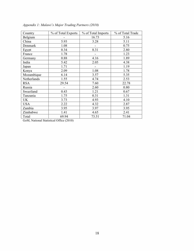
were converted to US dollar equivalents at the officially supplied exchange rates. Appendix 1 shows
Malawi’s nineteen most important trading partners which accounted for about 71 percent of Malawi’s
total trade in 2010. Of these, adequate data were not available for Mozambique, Swaziland and
Zimbabwe, such that the income level of Malawi’s trading partners (!!∗), expressed in US$ terms, was
computed as the sum of the nominal GDPs of the remaining sixteen trading partners.
The study used quarterly data for the period 1980Q1 – 2010Q2. Most of the data used were
obtained from the IMF’s International Financial Statistics (IFS) online database, but data gaps were filled
through recourse to various issues of the Financial and Economic Review of the Reserve Bank of Malawi
and other online data sources, and through interpolation. Importantly, since GDP data did not exist at the
quarterly frequency for many countries including Malawi, or only existed for part of the sampling period
for other countries, they were interpolated with the use of individual countries’ export values as follows:
tTi
tTi TiTi
XY YX
= (5)
where tTiY and tTiX are the GDP and export values in quarter t of year T for country i, while TiY and TiX
are the GDP and export values for country i in year T. Although this interpolation process is not error-free
(and none is!), the data thus generated alongside cases where actual quarterly GDP series were available
had much smaller discrepancies compared with using the alternative index of industrial production (IIP)
in place of export values. In addition, this process was preferred since the sum of quarterly export values
is a meaningful statistic as opposed to the sum of quarterly IIP observations.
The foregoing discussion indicates that the data were compiled on five variables, namely the
value of Malawi’s exports ( X ), the value of Malawi’s imports (M ), the GDP in Malawi (Y ), the total
GDP of Malawi’s trading partners ( *Y ) as well as Malawi’s real effective exchange rate ( E ). Time plots
of the natural logarithms of the five variables are presented in Appendix 2. It is reasonable to suspect that
seasonality was prevalent in some of the series. To address this, the following regression was fitted on
each of the five variables:
1 2 2 3 3 4 4t t t t tV d d dψ ψ ψ ψ υ= + + + + (6)
where tV is the series being tested for seasonality, jtd assumes a value of unity in the jth quarter of the
year and zero otherwise, and jψ are parameters to be estimated. Seasonal effects were said to be
prevalent if at least one of the jψ coefficients was significant at 5 percent significance level. The results

10
of this procedure revealed that seasonal effects were in fact present in the tX and the tY series, but not in
the rest. The evident seasonality was eliminated by noting that the corresponding t̂υ series represented
the deseasonalised tV series in such instances.
Further to the above, all the variables except the real effective exchange rate also showed an
upward trend which could potentially be deterministic. A downward deterministic trend in the exchange
rate (consistent with persistent depreciation of the Malawi kwacha in real terms) could also be suspected.
The effect of currency floatation was also noticeable through a downward spike which reached its floor
during the last quarter of 1994, but this effect clearly died off within 1994. Based on these observations,
and since currency flotation occurred in the 1994Q1, the study attempted to include the trend and
intercept terms, and a dummy variable which assumed a value of unity for all 1994 observations and zero
otherwise. However, the estimated coefficients of the trend term and the currency floatation dummy
variable were persistently insignificant at 5 percent. Therefore only the intercept terms were included in
the final models in order to avoid undue loss of degrees of freedom. In the ensuing analysis, the intercepts
for the two models are denoted a and b , respectively. All the estimations and tests were conducted using
the EViews 7 package.
5. Results and Discussion
5.1 Model specifications and diagnostics
The results of the lag order selection process for differenced terms as well as the B-G LM tests
are presented in Table 3 for both the export value model (Panel A) and the import value model (Panel B).
While both the SBC and HQC suggested a lag of 1 for the export value model, the resulting regression
was unable to account for serial correlation. Similarly, some evidence of first order serial correlation was
apparent (although only at 10 percent significance level) in the 2-lag model suggested by the AIC. A lag
order of three was acceptable in terms of accounting for serial correlation, despite that it was not preferred
by any of the three criteria. Similarly, the parsimonious one-lag import value model suggested by the
SBC and HQC showed signs of serial correlation that was effectively corrected through the inclusion of
three lags instead of one, but adding a forth lag appeared rather unrewarding in terms of the serial
correlation structure. Therefore, three lags in differenced terms were included in both models.
Table 3: Model selection statistics Panel A: Export value model
Lag Selection Criteria Statistics B-G LM Test AIC SBC HQC 21χ (p) 2
4χ (p) 1 0.241 0.412* 0.315* 0.306 (0.083) 12.400 (0.015) 2 0.233* 0.466 0.328 3.611 (0.057) 5.693 (0.223)

11
3 0.251 0.556 0.375 1.976 (0.160) 4.912 (0.296) 4 0.287 0.665 0.440 1.589 (0.207) 10.925 (0.027)
Panel B: Import value model Lag Selection Criteria Statistics B-G LM Test AIC SBC HQC 2
1χ (p) 24χ (p)
1 -0.181 -0.018* -0.115* 1.236 (0.266) 16.862 (0.002) 2 -0.186 0.047 -0.090 6.907 (0.009) 9.888 (0.042) 3 -0.215 0.091 -0.091 0.268 (0.605) 4.294 (0.368) 4 -0.219* 0.159 -0.065 2.448 (0.118) 2.950 (0.566)
Notes: 21χ
and 24χ are the B-G LM test statistics under the null hypotheses of no 1st order and 4rd order serial correlation
respectively, and (p) denotes the corresponding probabilities of accepting such null hypotheses. * identifies the suggested model under each criterion.
Table 4 shows that Ramsey’s RESET yielded insignificant statistics at the 5 percent significance
level for the two regression models investigated, suggesting that there were no gulling signs of incorrect
functional form. On the other hand, the ARCH test suggested the presence of conditional
heteroscedasticity in the import value model but not the export value model. Therefore, the export value
regression was estimated using the ordinary least squares (OLS) method, while the import value
regression was estimated as a first order generalised ARCH processes (that is, a GARCH (1,1) process) to
account for the observed ARCH effects. Maximum likelihood estimation was accomplished in estimating
the latter model by employing the Marquadt optimisation algorithm. The estimated GARCH model
showed that the resultant error terms were conditionally normally distributed – the Jarcque-Bera test
statistic yielded a probability value of 0.727 – implying that there was no necessity for invoking quasi-
maximum likelihood assumptions and generating robust standard errors and covariances, as would be
required if conditional normality did not hold. Moreover, setting a smoothing parameter of 0.8 in
backcasting the pre-sample variance for GARCH seemed conservatively reasonable: the conclusions
reported in this paper were sturdily strengthened as this value approached unity (that is, as the assumed
pre-sample variance approached the unconditional variance).
Table 4: Diagnostic tests for selected models
Model Ramsey’s RESET Test Engel’s ARCH Test F2 (p) F3 (p) 2
1χ (p) 24χ (p)
Export value 0.682 (0.411) 0.514 (0.599) 0.030 (0.864) 1.844 (0.764) Import value 0.659 (0.419) 0.547 (0.581) 1.504 (0.220) 14.903 (0.005)*
Notes: F2 and F3 are the test statistics for investigating the appropriateness of quadratic and cubic models, respectively. Similarly 21χ
and 24χ are the test statistics for ARCH(1) and ARCH(4) effects, respectively. In each case, (p) denotes the corresponding
probability value under the respective null hypotheses of correct specification or no conditional heteroscedasticity. * indicates that the appropriate null hypothesis may be rejected at 5% significance level.
Full estimation results are presented in Table 5, in which Panel A shows the results of estimating
the export value regression model, while Panel B shows similar results for the import value model. The

12
models only explained 26 percent and 17 percent of the variability in the values of exports and imports,
providing prima facie evidence against the validity of the underlying theories. The sturdily significant
GARCH term coefficient buttressed the observation of ARCH effects in the import value model. Results
for formal tests of the long-run and short-run exchange rates effects on trade are analysed in the sequel.
Table 5: Estimation Results
Panel A: Export value model Panel B: Import value model Variable Coefficient t-Statistic Prob. Variable Coefficient t-Statistic Prob.
a 0.303 0.168 0.867 b 2.571 2.338 0.019 ΔLnXt-1 -0.237 -1.961 0.053 ΔLnMt-1 -0.190 -1.048 0.295 ΔLnXt-2 -0.309 -2.874 0.005* ΔLnMt-2 -0.347 -2.399 0.016 ΔLnXt-3 -0.170 -1.662 0.100 ΔLnMt-3 -0.190 -1.678 0.093 Δ LnY*t-1 -1.413 -1.376 0.172 Δ LnYt-1 -0.010 -0.076 0.940 Δ LnY*t-2 -1.526 -1.774 0.079 Δ LnYt-2 0.069 0.765 0.444 Δ LnY*t-3 -0.591 -0.699 0.486 Δ LnYt-3 -0.077 -1.032 0.302 ΔlnEt-1 0.402 1.761 0.081 ΔlnEt-1 -0.111 -0.353 0.724 ΔlnEt-2 -0.138 -0.527 0.599 ΔlnEt-2 0.577 1.746 0.081 ΔlnEt-3 0.154 0.501 0.617 ΔlnEt-3 0.331 1.111 0.267 LnXt-1 -0.334 -2.863 0.005* LnXt-1 -0.117 -1.003 0.316 LnY*t-1 0.117 1.0516 0.295 LnYt-1 -0.044 -0.367 0.714 LnEt-1 -0.267 -1.463 0.146 LnEt-1 -0.395 -2.965 0.003
Variance equation 2R = 0.259 Intercept 0.002 1.095 0.274 F = 4.409 ARCH(1) 0.170 1.473 0.141
Prob (F) = 0.000 GARCH(1) 0.790 5.829 0.000 2R = 0.171
Note: * denotes statistical significance before any normalisation procedures, at 5% significance level or lower.
5.3 Long-run effects Cointegation test results under the aforesaid null hypotheses are summarised in Table 6. The
critical values used were from Pesaran et al. (2001), as presented in their Table C1.iii. In both models, the
test statistics fell in the region between the lower bound and upper bound critical values at the 5 percent
significance level, suggesting that the test was inconclusive. While this did not suggest a rejection of the
cointegration hypothesis per se, it did not suggest evidence of the same either. However, at the 10 percent
significance level, some weak evidence of cointegration was prevalent in the export value model, and the
test statistic for the import value model was notably much closer to the upper bound critical value than it
was to the lower bound critical value. The inconclusive test result, therefore, seemed to tilt more towards
not rejecting cointegration rather than rejecting it.
Table 6: Cointegration Test Results

13
Model Null Hypothesis F-Statistic 5% Critical Values 10% Critical Values CVL CVU CVL CVU
Export value 1 2 3 0φ φ φ= = = 3.866 3.23 4.35 2.72 3.77
Import value 1 2 3 0ϕ ϕ ϕ= = = 3.230 3.23 4.35 2.72 3.77
Note: CVL and CVU are the lower bound and upper bound critical values provided by Pesaran et al. (2001).
Subject to the admissibility of this vacillating evidence of cointegration, the long-run sensitivities
of export and import values to the real effective exchange rate were established through normalisation, as
follows:
Export value model: -0.798
Import value model: -3.379
These normalised effects appeared large, but should obviously be interpreted within the context
of statistical significance. The 21χ Wald test statistics computed under the null hypotheses that
3 1 0φ φ− = and 3 1 0ϕ ϕ− = were respectively equal to 1.585 and 1.360, with probability values of
0.208 and 0.244. This suggested that there were no significant long-run effects of the real effective
exchange rate on either export values or import values, which was consistent with the observation that
cointegration could not be unequivocally established in the first place. Although the lnEt-1 coefficient was
significant in the import value model, it follows that this result was more spurious than credible.
5.3 Short-run effects
Table 5 above shows that all the first differences of the real effective exchange rate were
insignificant at the 5 percent significance level in both the export value model and the import value model
(although there were traces of statistical significance at 10 percent), and that a key source of the scanty
explanatory power in the models was autoregressive terms and non-normalised (spurious) long-run
effects.
In the spirit of Granger-causality testing, the joint significance of each exogenous variable’s
lagged difference terms was evaluated as reported in Table 7. Clearly, the real effective exchange rate
terms were completely unimportant (as were the income variable terms) in explaining both export values
and import values.
Table 7: Joint short-run effects Panel A: Export value model
Effect Null Hypothesis F-Statistic (p) Own 1 2 3 0ρ ρ ρ= = = 2.830 (0.042

14
Trade partners’ GDP 1 2 3 0δ δ δ= = = 1.599 (0.194)
Exchange rate 1 2 3 0π π π= = = 1.210 (0.310) Panel B: Import value model
Effect Null Hypothesis F-Statistic (p) Own 1 2 3 0γ γ γ= = = 1.995 (0.119)
Malawi’s GDP 1 2 3 0λ λ λ= = = 1.449 (0.233)
Exchange rate 1 2 3 0η η η= = = 1.461 (0.230) Note: (p) denoted the probability of accepting the corresponding null hypothesis of joint insignificance. * denotes statistical significance at 5% or lower.
6. Conclusion
This study jointly examined the effects of the exchange rate on the aggregate trade balance in
Malawi. Both the long-run effects postulated in the Marshall-Lerner condition, as well as the short-run
effects proposed by the J-curve theory were simultaneously explored. Separate export value and import
value models were estimated using the single equation error correction modelling framework proposed by
Pesaran et al. (2001). Apart from the real effective exchange rate, the aggregate GDP of Malawi’s key
trading partners was included in the export value function, while Malawi’s own GDP was allowed to
explain the value of imports. The inclusion of a dummy variable to account for foreign exchange
liberalisation in 1994 was unrewarding in both models. Similarly, the inclusion of a trend term was found
to be gratuitous, even though this was suggested in a graphical display of the series.
The findings documented in the paper show that the trade balance in Malawi was not sensitive to
the real effective exchange rate, both in the long-run and in the short-run. Evidence of a long-run
(equilibrium) relationship could not be forcefully established in either the export value or the import value
models. Even when this was optimistically assumed, the normalised exchange rate elasticities of export
values and import values were not significantly different from zero. Similarly, the exchange rate variable
did not have any short-run effects on export values or import values, both of which were scantily
explained by their own lagged values in the short run.
That the trade balance in Malawi was not sensitive to movements in the real effective exchange
rate is explainable from an examination of the constituents of exports and imports. Tobacco was Malawi’s
dominant export, accounting for 59.5 percent of the value of Malawi’s total exports in 2010 according to
the Government of Malawi’s National Statistical Office (see http://www.nso.malawi.net). Uranium had
recently become a distant second at 11.6 percent of export value in 2010, followed by tea at 8 percent.
Tobacco production was entrenched in the economy of Malawi to the point that it could not respond to
changes in world prices, let alone exchange rates which were generally fixed in nominal terms. The so-

15
called cobweb phenomenon in agricultural production suggested that the time lag with which even the
most rational farmers could react to changing market conditions was generally long, and a significant
proportion of tobacco production in Malawi was by smallholder farmers with limited options and
constrained flexibility in decision-making. Similar arguments could be made regarding the rest of
Malawi’s key exports. On the other hand, the country’s imports tended to be dominated by necessities.
Fertilizers were most dominant, and accounted for 14.4 percent of the total import bill in 2010, followed
by petroleum products (14.0 percent) and medicines (7.1 percent). Significant amounts of the import bill
were also attributable to machinery plant and laboratory equipment. It is overly presumptuous to expect
that such imports should be responsive exchange rate changes.
The findings of this study suggest that exchange rate policy should focus more on other national
considerations (such as influencing imported inflation) than the trade balance. They particularly support a
contentious proposition that exchange rate policy can be applied to achieve welfare maximisation at
hardly any opportunity cost of deterioration in the trade balance. The results also suggest that the
country’s persistently precarious foreign reserve position is a result more of the unavailability of adequate
reserves than the effect of currency overvaluation on trade.
It is possible that the results reported in this paper are a construct of aggregation bias, implying
that a study of bilateral trade flows between Malawi and its individual trading partners might yield
different results. Potentially different results could also obtain if the responsiveness of key individual
imports and exports (as opposed to aggregates) were explored. Such reasoning could inform the direction
of subsequent research.
References
Arize, A.C., 2001. Traditional export demand relation and parameter stability: an empirical investigation.
Journal of Economic Studies 28, 378-398.
Bahmani-Oskooee, M., 1985. Devaluation and the J-curve: some evidence from LDCs. The Review of
Economics and Statistics, 500-504.
Bahmani-Oskooee, M., 1991. Is there a long-run relation between the trade balance and the real effective
exchange rate of LDCs? Economics Letters 36, 403-407.
Bahmani-Oskooee, M., and Goswami, G., 2004. Exchange rate sensitivity of Japan’s bilateral trade flows,
Japan and the World Economy 16, 1-15.
Bahmani-Oskooee, M., and Ratha, A, 2004. The J-curve: a literature review. Applied Economics 36,
1377-98.
Bahmani-Oskooee, M., and Ratha, A, 2008. Exchange rate sensitivity of US bilateral trade flows.
Economic Systems 32, 129-141.

16
Bickerdike, C.F., 1920. The instability of foreign exchanges. The Economic Journal, March.
Cassel, G., 1918. Abnormal deviations in international exchanges. Journal, December, 413-415
Government of Malawi, 2011. Government of Malawi Budget Statement 2011-12. Lilongwe: Ministry of
Finance.
Government of Malawi, various. Annual Economic Report. Lilongwe: Ministry of Development Planning
and Cooperation.
Gupta-Kapoor, A., and Ramakrishna, U., 1999. Is there a J-curve? A new estimation for Japan.
International Economic Journal 13(4), 71-89.
Hsing, H., 1999 in Kamoto, E., 2006. The J-Curve Effect on the Trade Balance in Malawi and South
Africa. MA Thesis, The University of Texas at Arlington.
http://www.nso.malawi.net, International Merchandise Trade Statistics. Zomba: National Statistica Office
of Malawi. Downloaded on 20 July 2011.
Junz, H.B., and Romberg, R.R., 1973. Price competitiveness in export trade among industrial countries.
American Economic Review 3, 314-327.
Kamoto, E., 2006. The J-Curve Effect on the Trade Balance in Malawi and South Africa. MA Thesis, The
University of Texas at Arlington.
Koch, P., and Rosensweig, J., 1990. The dynamic relationship between the dollar and the components of
US trade. Journal of Business and Economic Statistics 8(3), 355-364.
Lerner, A.P., 1944. The Economics of Control: Principles of welfare Economics. New York: MacMillan.
Magee, S., 1973. Currency contracts, pass-through, and devaluation. Brookings Papers of Economic
Activity 1, 303-323.
Malawi Savings Bank, 2011. Financial and Economic Report for January 2011. Blantyre: Malawi Savings
Bank Limited.
Mangani, R., 2011. The effects of monetary policy on prices in Malawi. AERC Research Paper, African
Economic Research Consortium (forthcoming).
Marshall, A., 1923. Money, Credit and Currency. London: MacMillan.
Metzler, L., 1948. A Survey of Contemporary Economics Vol 1. Illinois: Irwin.
Nadenichek, J., 2000. The Japan-US trade imbalance: a real business cycle perspective. Japan and the
World Economy 12, 255-271.
Narayana, S., and Narayana, P.K., 2005. An empirical analysis of Fiji’s import demand function. Journal
of Economic Studies 32, 158-168.
Ngalawa, H., 2009. Dynamic effects of monetary policy shocks in Malawi. Conference paper, 14th Annual
Conference of the African Econometrics Society. Abuja

17
Onafowora, O., 2003. Exchange rate and trade balance in East Asia: is there a J-curve? Economic Bulletin
5(18), 1-13.
Pesaran, H.M., Shin, Y., and Smith, R.J., 2001. Bounds testing approach to the analysis of level
relationships. Journal of Applied Economics 16, 289-326.
Reserve Bank of Malawi, 2009. Monthly Economic Review, July 2009. Lilongwe: Reserve Bank of
Malawi.
Reserve Bank of Malawi, various. Financial and Economic Review. Lilongwe: Reserve Bank of Malawi.
Robinson, J., 1947. Essays in the Theory of Employment. Oxford: Basil Blackwell.
Summary, R.M., 1989. A political-economy model of US bilateral trade. Review of Economics and
Statistics 71, 179-182.
Tihomir, S., 2004. The effects of exchange rate change on the trdae balance in Croatia. IMF Working
Papers 04(65).
18
Appendix 1: Malawi’s Major Trading Partners (2010) Country % of Total Exports % of Total Imports % of Total Trade Belgium - 16.73 5.16 China 5.93 3.28 5.11 Denmark 1.08 - 0.75 Egypt 0.34 8.31 2.80 France 1.78 - 1.23 Germany 0.88 4.16 1.89 India 5.42 2.05 4.38 Japan 1.71 - 1.19 Kenya 2.09 1.08 1.78 Mozambique 6.14 3.57 5.35 Netherlands 1.55 4.74 2.53 RSA 29.54 7.60 22.78 Russia - 2.60 0.80 Swaziland 0.43 1.21 0.67 Tanzania 1.75 0.31 1.31 UK 3.73 4.93 4.10 USA 2.22 4.32 2.87 Zambia 3.95 3.97 3.95 Zimbabwe 1.41 4.65 2.41 Total 69.94 73.51 71.04 GoM, National Statistical Office (2010)

19
Appendix 2 – Time Plots of the Variables (in Natural Logarithmic Form)
3.5
4.0
4.5
5.0
5.5
6.0
6.5
1980 1985 1990 1995 2000 2005 20105.0
5.5
6.0
6.5
7.0
7.5
1980 1985 1990 1995 2000 2005 2010
8.0
8.4
8.8
9.2
9.6
10.0
10.4
1980 1985 1990 1995 2000 2005 20103.5
4.0
4.5
5.0
5.5
6.0
6.5
7.0
1980 1985 1990 1995 2000 2005 2010
4.4
4.6
4.8
5.0
5.2
5.4
5.6
1980 1985 1990 1995 2000 2005 2010
LnX LnY
LnY* lnM
LnE