Embed Size (px)
Citation preview

Robust Model Predi tive Control of an Ele tri Ar Furna e Rening Pro essbyLodewi us Charl CoetzeeSubmitted in partial fullment of the requirements for the degreeMaster of Engineering (Ele troni Engineering)in theFa ulty of Engineering, the Built Environment andInformation Te hnologyUNIVERSITY OF PRETORIAJune 28, 2006

SummaryTitle: Robust Model Predi tive Control of an Ele tri Ar Furna eRening Pro essBy: Lodewi us Charl CoetzeeSupervisor: Professor I.K. CraigDepartment: Department of Ele tri al, Ele troni and Computer EngineeringDegree: Master of Engineering (Ele troni Engineering)This dissertation forms part of the ongoing pro ess at UP to model and ontrol theele tri ar furna e pro ess. Previous work fo used on modelling the furna e pro ess fromempiri al thermodynami prin iples as well as tting the model to a tual plant data.Automation of the pro ess mainly fo used on subsystems of the pro ess, for example theele tri subsystem and the o-gas subsystem.The modelling eort, espe ially the model tting, resulted in parameter values that aredes ribed with onden e intervals, whi h gives rise to un ertainty in the model, be ausethe parameters an potentially lie anywhere in the onden e interval spa e.Robust model predi tive ontrol is used in this dissertation, be ause it an expli itlytake the model un ertainty into a ount as part of the synthesis pro ess. Nominal modelpredi tive ontrol - not taking model un ertainty into a ount - is also applied in orderto determine if robust model predi tive ontrol provides any advantages over the nominalmodel predi tive ontrol.This dissertation uses the pro ess model from previous work together with robustmodel predi tive ontrol to determine the feasibility of automating the pro ess with re-gards to the primary pro ess variables. Possible hurdles that prevent pra ti al implemen-tation are identied and studied.Keywords: Ele tri Ar Furna e, Robust Model Predi tive Control, EAF, RMPC.

OpsommingTitel: Robuuste Model Voorspellende Beheer van 'n Elektriese BoogoondVerfyningsprosesDeur: Lodewi us Charl CoetzeeStudieleier: Professor I.K. CraigDepartement: Departement van Elektries, Elektronies and Rekenaar IngenieursweseGraad: Meester van Ingenieurswese (Elektroniese Ingenieurswese)Die verhandeling vorm deel van die voortgaande studie deur UP om 'n elektriese boo-goondproses te modelleer en te beheer. Vorige modellering het gefokus op die gebruik vanempiriese termodinamiese beginsels waarna die empiriese model gepas is op gemete aan-legdata. Outomatisasie word hoofsaaklik gemik op substelsels van die proses, byvoorbeelddie elektriese substelsel.Die modelleringsproses, veral die passing van die model op aanlegdata, het daartoegelei dat daar onsekerhede in die model vervat word. Die onsekerhede word beskryf deurparameters wat binne vasgestelde grense lê.In die verhandeling word robuuste model voorspellende beheer gebruik, omdat dit dieonsekerhede van die aanleg eksplisiet in ag kan neem gedurende die sinteseproses. Dierobuuste beheerder word vergelyk met 'n nominale beheerder - wat nie die onsekerhedein ag neem nie - om te bepaal watter voordeel die robuuste beheerder oor die nominalebeheerder bied.Die aanlegmodel, wat in 'n vorige studie verkry is, tesame met robuuste model voor-spellende beheerteorie word gebruik om te bepaal hoe haalbaar dit is om die elektrieseboogoondverfyningsproses te outomatiseer. Die studie het moontlike struikelblokke geï-dentiseer wat praktiese implementering kan belemmer.Sleutelwoorde: Elektriese Boogoond, Robuuste Model Voorspellende Beheer.

A knowledgementI thank God for blessing me with the opportunity to study. I owe my parents a debtof gratitude for their support and understanding throughout my studies. I thank mysupervisor Prof. Craig for his guidan e and help with this resear h and Mr. Bellinganfrom Cape Gate for his insight in the pra ti al operation of an ele tri ar furna e.

Contents1 Introdu tion 11.1 Motivation . . . . . . . . . . . . . . . . . . . . . . . . . . . . . . . . . . . . 11.2 Operation of the Ele tri Ar Furna e . . . . . . . . . . . . . . . . . . . . . 21.3 Aims and obje tives . . . . . . . . . . . . . . . . . . . . . . . . . . . . . . 91.4 Organization . . . . . . . . . . . . . . . . . . . . . . . . . . . . . . . . . . 102 Pro ess modelling 122.1 Introdu tion . . . . . . . . . . . . . . . . . . . . . . . . . . . . . . . . . . . 122.2 Redu ed Nonlinear Model . . . . . . . . . . . . . . . . . . . . . . . . . . . 152.3 Predi tor design . . . . . . . . . . . . . . . . . . . . . . . . . . . . . . . . . 182.4 Linearized model . . . . . . . . . . . . . . . . . . . . . . . . . . . . . . . . 202.4.1 Operating point . . . . . . . . . . . . . . . . . . . . . . . . . . . . . 212.4.2 Derivative of nonlinear model . . . . . . . . . . . . . . . . . . . . . 222.4.3 Linearized models . . . . . . . . . . . . . . . . . . . . . . . . . . . . 262.4.4 Linear models analysis . . . . . . . . . . . . . . . . . . . . . . . . . 292.4.5 Simpli ation of linear models . . . . . . . . . . . . . . . . . . . . . 312.4.6 Analysis of simplied linear models . . . . . . . . . . . . . . . . . . 352.5 Con lusion . . . . . . . . . . . . . . . . . . . . . . . . . . . . . . . . . . . . 353 Model predi tive ontrol 373.1 Introdu tion . . . . . . . . . . . . . . . . . . . . . . . . . . . . . . . . . . . 373.2 Histori al ba kground . . . . . . . . . . . . . . . . . . . . . . . . . . . . . . 413.3 Stability of MPC . . . . . . . . . . . . . . . . . . . . . . . . . . . . . . . . 43ii

CONTENTS3.3.1 Stability onditions for model predi tive ontrollers . . . . . . . . . 443.3.2 Terminal state MPC . . . . . . . . . . . . . . . . . . . . . . . . . . 473.3.3 Terminal ost MPC . . . . . . . . . . . . . . . . . . . . . . . . . . . 483.3.4 Terminal onstraint set MPC . . . . . . . . . . . . . . . . . . . . . 483.3.5 Terminal ost and onstraint set MPC . . . . . . . . . . . . . . . . 493.4 Robust MPC - Stability of un ertain systems . . . . . . . . . . . . . . . . . 503.4.1 Stability onditions for robust MPC . . . . . . . . . . . . . . . . . . 513.4.2 Open-loop min-max MPC . . . . . . . . . . . . . . . . . . . . . . . 523.4.3 Feedba k robust MPC . . . . . . . . . . . . . . . . . . . . . . . . . 543.4.4 Robust MPC implementations . . . . . . . . . . . . . . . . . . . . . 563.5 Robust model predi tive ontrollers . . . . . . . . . . . . . . . . . . . . . . 583.5.1 Robust MPC using LMIs . . . . . . . . . . . . . . . . . . . . . . . . 583.5.1.1 System des riptions . . . . . . . . . . . . . . . . . . . . . 593.5.1.2 Obje tive fun tion . . . . . . . . . . . . . . . . . . . . . . 603.5.1.3 Linear matrix inequalities . . . . . . . . . . . . . . . . . . 613.5.1.4 Un onstrained robust model predi tive ontrol . . . . . . . 613.5.1.5 Input onstraints . . . . . . . . . . . . . . . . . . . . . . . 633.5.1.6 Output onstraints . . . . . . . . . . . . . . . . . . . . . . 643.5.1.7 Synthesis of the ontroller . . . . . . . . . . . . . . . . . . 653.5.1.8 Controller operation . . . . . . . . . . . . . . . . . . . . . 653.5.2 Dual-mode robust model predi tive ontroller . . . . . . . . . . . . 663.5.2.1 Augmented system des ription . . . . . . . . . . . . . . . 663.5.2.2 Constraints of the augmented system . . . . . . . . . . . . 663.5.2.3 Quadrati problem weighting matrix . . . . . . . . . . . . 663.5.2.4 On-line ontrol problem . . . . . . . . . . . . . . . . . . . 673.5.2.5 Synthesis of ontroller . . . . . . . . . . . . . . . . . . . . 673.5.2.6 Controller operation . . . . . . . . . . . . . . . . . . . . . 683.6 Con lusion . . . . . . . . . . . . . . . . . . . . . . . . . . . . . . . . . . . . 68Ele tri al, Ele troni and Computer Engineering iii

CONTENTS4 Simulation Study 704.1 Introdu tion . . . . . . . . . . . . . . . . . . . . . . . . . . . . . . . . . . . 704.1.1 Controller weighting matri es . . . . . . . . . . . . . . . . . . . . . 714.1.2 Closed-loop ar hite tures . . . . . . . . . . . . . . . . . . . . . . . . 724.1.3 Controller obje tives . . . . . . . . . . . . . . . . . . . . . . . . . . 734.1.4 Typi al operation . . . . . . . . . . . . . . . . . . . . . . . . . . . . 754.2 Nominal S enario . . . . . . . . . . . . . . . . . . . . . . . . . . . . . . . . 764.3 Worst- ase s enario: E ien ies at their minimum . . . . . . . . . . . . . . 784.3.1 Full state feedba k . . . . . . . . . . . . . . . . . . . . . . . . . . . 884.3.2 One plant measurement . . . . . . . . . . . . . . . . . . . . . . . . 894.3.3 One plant measurement with predi tor update . . . . . . . . . . . . 984.4 Worst- ase s enario: E ien ies at their maximum . . . . . . . . . . . . . 1034.4.1 Full state feedba k . . . . . . . . . . . . . . . . . . . . . . . . . . . 1034.4.2 One plant measurement . . . . . . . . . . . . . . . . . . . . . . . . 1044.5 Temperature disturban e . . . . . . . . . . . . . . . . . . . . . . . . . . . . 1094.6 Summary . . . . . . . . . . . . . . . . . . . . . . . . . . . . . . . . . . . . 1164.7 Con lusion . . . . . . . . . . . . . . . . . . . . . . . . . . . . . . . . . . . . 1175 Con lusions and re ommendations 1245.1 Summary of dissertation . . . . . . . . . . . . . . . . . . . . . . . . . . . . 1245.2 Con lusion . . . . . . . . . . . . . . . . . . . . . . . . . . . . . . . . . . . . 1255.3 Further work . . . . . . . . . . . . . . . . . . . . . . . . . . . . . . . . . . 126Referen es 129A A ademi Problem 138A.1 A ademi problem model . . . . . . . . . . . . . . . . . . . . . . . . . . . . 138A.2 Simulation Results . . . . . . . . . . . . . . . . . . . . . . . . . . . . . . . 140A.2.1 Nominal s enario . . . . . . . . . . . . . . . . . . . . . . . . . . . . 141A.2.2 Extreme deviation δ = −1 and δ = 1 . . . . . . . . . . . . . . . . . 144A.3 Con lusion . . . . . . . . . . . . . . . . . . . . . . . . . . . . . . . . . . . . 144Ele tri al, Ele troni and Computer Engineering iv

CONTENTSB Auxiliary simulation results 149B.1 Worst- ase s enario: E ien ies at their minimum . . . . . . . . . . . . . . 149B.1.1 Full state feedba k . . . . . . . . . . . . . . . . . . . . . . . . . . . 150B.1.2 One plant measurement . . . . . . . . . . . . . . . . . . . . . . . . 154B.1.3 One plant measurement with predi tor update . . . . . . . . . . . . 158B.2 Worst- ase s enario: E ien ies at their maximum . . . . . . . . . . . . . 158B.2.1 Full state feedba k . . . . . . . . . . . . . . . . . . . . . . . . . . . 163B.2.2 One plant measurement . . . . . . . . . . . . . . . . . . . . . . . . 168B.2.3 One plant measurement with predi tor update . . . . . . . . . . . . 175C Measured bath and slag data 183
Ele tri al, Ele troni and Computer Engineering v
List of abbreviationsANN Arti ial Neural NetworkBOF Basi Oxygen Furna eDMC Dynami Matrix ControlDRI Dire t Redu ed IronDRMPC Dual-mode Robust Model Predi tive ControlEAF Ele tri Ar Furna eFRMPC Feedba k Robust Model Predi tive ControlGPC Generalized Predi tive ControlIDCOM Identi ation and CommandLMI Linear Matrix InequalitiesMPC Model Predi tive ControlODE Ordinary Dierential EquationQP Quadrati ProgrammingRHC Re eding Horizon ControlRMPC Robust Model Predi tive ControlSCADA Supervisory Control And Data A quisitionSDP Semidenite ProgrammingSMOC Shell Multi-variable Optimizing ControlUP University of Pretoriavi

List of symbolsList of Chemi al SymbolsC CarbonCaO Cal ium OxideCO Carbon monoxideFeO Iron OxideMgO Magnesium OxideMnO Manganese OxideP2O5 Phosphorus OxideSi Sili onSiO2 Sili on DioxideNonlinear model symbolsNonlinear model statesx3 Carbon ontent in bath [kgx4 Sili on ontent in bath [kgx7 FeO ontent in slag [kgx8 SiO2 ontent in slag [kgx12 Bath and molten slag temperature [0Cvii

List of symbolsNonlinear model inputsd1 Rate of oxygen inje tion [kg/sd2 Rate of DRI addition [kg/sd3 Rate of slag forming additions [kg/sd4 Ele tri power [kWd5 Rate of graphite inje tion [kg/sNonlinear model outputsy1 Bath and molten slag temperature [0Cy2 Per entage arbon in bath [%y3 FeO ontent in slag [kgNonlinear model parametersCp(k) Heat apa ity of element / ompound k [kJ/(mol.K)Mk Molar mass of element / ompound k [kg/molXk Mole fra tion of element / ompound k
Xeqk Equilibrium mole fra tion of element / ompound k
∆Hk Enthalpy of formation of ompound k [kJ/molTk Initial temperature of element / ompound k [KkXC Equilibrium on entration onstant for arbonkXSi Equilibrium on entration onstant for sili onkdC De arburization rate onstant [kg/skdSi Desili onization rate onstant [kg/skgr Graphite rea tivity onstantkV T EAF heat loss oe ientηFeO E ien y of bath oxidationηARC E ien y of ar power inputEle tri al, Ele troni and Computer Engineering viii

Chapter 1Introdu tionThis hapter provides a motivation for the the study undertaken in this dissertation. Ashort overview of the ele tri ar furna e pro ess is given, followed by an explanation of the ontribution of this dissertation as well as the organization of the rest of the dissertation.1.1 MotivationWith the growth of the world e onomies, the demand on natural resour es is growing. Ironore is no dierent, and like most natural resour es, it is not renewable. The solution is toreuse old materials through re y ling in order to redu e the demand for natural resour es.The use of ele tri ar furna es (EAFs) is an important part of the re y ling eort in thesteel industry. EAFs are apable of melting down solid s rap metal and rening it to therequired steel grade by manipulating the hemi al properties of the steel. The ele tri ar furna e is slowly repla ing the basi oxygen furna e (BOF) (IISI, 2003), be ause ituses hemi al as well as ele tri al energy to melt the s rap metal. The ele tri al energyis introdu ed by three arbon ele trodes that form an ele tri ar between them thatradiates heat to the metal. Chemi al energy is primarily provided by natural gas andoxygen.The ele tri ar furna e pro ess is still heavily dependent on operator ontrol. Theoperator uses a re ipe based on initial measurements of the hemi al omposition todetermine how long ele tri al power should be applied, as well as how mu h oxygen,1

Chapter 1 Operation of the Ele tri Ar Furna e arbon and other additives should be added. The melting time is often based on a feelfor the pro ess and the sound emanating from the furna e. Measurements are takenintermittently to gauge the progress and to make adjustments as needed. This leads tovarying su ess in obtaining the desired steel grade.The pro ess ould benet hugely from the use of better automation to in rease energye ien y as well as to improve the onsisten y of the quality of the nal produ t byemploying good set-point following. Automation ould also improve the safety of thepro ess. Most of the urrent automation only fo uses on the parts of the pro ess thatultimately do not have a dire t inuen e on the grade of the steel produ ed.The mathemati al model of the ele tri ar furna e rening pro ess in ludes un er-tainty. Control of the pro ess requires that the ontroller needs to remain stable over allpossible realizations of the model while providing a eptable performan e. Robust modelpredi tive ontrol is well suited for un ertain multi-variable systems with onstraints,be ause it takes the model un ertainty expli itly into a ount as part of the synthesispro ess. The losed-loop system is guaranteed stable over all modelled realizations of theun ertain system. This makes robust model predi tive ontrol well suited as a ontrolmethod for the ele tri ar furna e rening pro ess.1.2 Operation of the Ele tri Ar Furna eThe ele tri ar furna e pro ess is on erned with melting s rap metal and produ ing steel.Ea h iteration of the pro ess is alled a tap. The time it takes to nish one iteration ofthe pro ess is alled the tap-to-tap time. One tap onsists of a few stages; harging thefurna e, melting down the s rap metal, rening the steel, removing the slag layer, tappingthe nished steel, and furna e turnaround. The ele tri ar furna e rening pro ess iswell des ribed by Taylor (1985); Fruehan (1998)Charging: Figure 1.1 shows a s hemati representation of an ele tri ar furna e that isbeing harged. Charging onsists of omposing a bu ket made up of s rap, other metalli elements and slag formers. The omposition of the s rap metal is dependent on thedesired grade of steel to be produ ed. The layering of the s rap is important: softer s rapEle tri al, Ele troni and Computer Engineering 2

Chapter 1 Operation of the Ele tri Ar Furna e
Hot Heel Level
Oxygen Injector
Graphite Injector
Carbon
Electrodes
Off-gas
Extraction Vent
Slag Door
Tap Hole
Removeable
Roof with Electrodes
Charge Bucket
Scrap
Scrap
Scra
p
Scrap
ScrapScrap
Figure 1.1: Ele tri ar furna e s hemati - Charging.
Ele tri al, Ele troni and Computer Engineering 3

Chapter 1 Operation of the Ele tri Ar Furna eis pla ed at the bottom of the bu ket, while harder s rap is loaded on top. The softers rap prote ts the furna e during harging and also melts down qui kly. The melted s rapforms a pool of molten metal that aids in melting the larger pie es. This physi al layeringshould prevent ave-ins from o urring, whi h ould damage the arbon ele trodes and ause a atastrophi breakdown. To harge the bu ket into the furna e, the roof of thefurna e swings away to expose the inside of the furna e. A rane positions the bu keton top of the furna e and the oor of the bu ket is opened to allow the s rap to fall intothe furna e. Some melt-shops only harge one bu ket and then add dire t redu ed iron(DRI) through hutes in the roof of the furna e. This requires extra infrastru ture su has a onveyor belt to transport the DRI to the hutes.The type of s rap used in harging will have an inuen e on the time of the meltdownstage. Light s rap melts down easily but does not ontain as mu h metal as denser,heavier s rap. More bu kets of light s rap will thus be ne essary to rea h the requiredmolten weight. With heavier s rap the melting pro ess takes longer, but less hargingneeds to be done. The danger with denser s rap is the potential for late ave-ins that andamage the ele trodes.Melting: Figure 1.2 shows a s hemati representation of an ele tri ar furna e in thepro ess of melting down the solid s rap. The roof of the furna e is swung ba k on topof the furna e. The roof ontains the three arbon ele trodes that are used to reate anele tri al ar . Melting is initiated by applying ele tri al power to the furna e's ele trodesas well as ring up the oxyfuel burners. The heat from the ar radiates towards the s rapto melt it down. A long ar between the ele trodes and s rap is sele ted during meltdown,be ause it radiates more heat over a greater area than a short ar . The ele tri ar boresa hole into the middle of the s rap heap, and as the hole is forming, the ele trodes arelowered into the hole. The surrounding s rap prote ts the furna e walls from the heatradiating from the ar . As the ele trodes bore into the s rap, a molten pool of metalforms, whi h prote ts the bottom of the furna e from the ar . The burners pro eed tomelt the metal at the edges of the furna e that are not rea hed by the ar .The use of oxyfuel burners and oxygen lan es do not guarantee that there will be noEle tri al, Ele troni and Computer Engineering 4

Chapter 1 Operation of the Ele tri Ar Furna e
Liquid Metal
Freeboard GassesOxygen Injector
Graphite Injector
Carbon
Electrodes
Off-gas
Extraction Vent
Slag Door
Tap Hole
Electric Arc
Removeable
Roof with
Electrodes
Scrap
Scrap
ScrapScrap
Scrap
Scrap
Scrap
Scrap
Figure 1.2: Ele tri ar furna e s hemati - Melting.Ele tri al, Ele troni and Computer Engineering 5
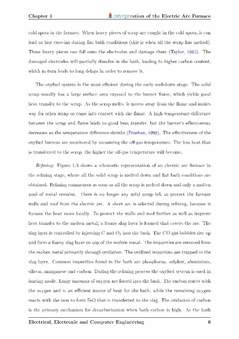
Chapter 1 Operation of the Ele tri Ar Furna e old spots in the furna e. When heavy pie es of s rap are aught in the old spots, it anlead to late ave-ins during at bath onditions (this is when all the s rap has melted).These heavy pie es an fall onto the ele trodes and damage them (Taylor, 1985). Thedamaged ele trodes will partially dissolve in the bath, leading to higher arbon ontent,whi h in turn leads to long delays in order to remove it.The oxyfuel system is the most e ient during the early meltdown stage. The solids rap usually has a large surfa e area exposed to the burner ame, whi h yields goodheat transfer to the s rap. As the s rap melts, it moves away from the ame and makesway for other s rap to ome into onta t with the ame. A high temperature dieren ebetween the s rap and ame leads to good heat transfer, but the burner's ee tivenessde reases as the temperature dieren e shrinks (Fruehan, 1998). The ee tiveness of theoxyfuel burners are monitored by measuring the o-gas temperature. The less heat thatis transferred to the s rap, the higher the o-gas temperature will be ome.Rening: Figure 1.3 shows a s hemati representation of an ele tri ar furna e inthe rening stage, where all the solid s rap is melted down and at bath onditions areobtained. Rening ommen es as soon as all the s rap is melted down and only a moltenpool of metal remains. There is no longer any solid s rap left to prote t the furna ewalls and roof from the ele tri ar . A short ar is sele ted during rening, be ause itfo uses the heat more lo ally. To prote t the walls and roof further as well as improveheat transfer to the molten metal, a foamy slag layer is formed that overs the ar . Theslag layer is ontrolled by inje ting C and O2 into the bath. The CO gas bubbles rise upand form a foamy slag layer on top of the molten metal. The impurities are removed fromthe molten metal primarily through oxidation. The oxidized impurities are trapped in theslag layer. Common impurities found in the bath are phosphorus, sulphur, aluminium,sili on, manganese and arbon. During the rening pro ess the oxyfuel system is used inlan ing mode. Large amounts of oxygen are for ed into the bath. The arbon rea ts withthe oxygen and is an e ient sour e of heat for the bath, while the remaining oxygenrea ts with the iron to form FeO that is transferred to the slag. The oxidation of arbonis the primary me hanism for de arburization when bath arbon is high. As the bathEle tri al, Ele troni and Computer Engineering 6

Chapter 1 Operation of the Ele tri Ar Furna e
Liquid Metal
Freeboard GassesOxygen Injector
Graphite Injector
Carbon
Electrodes
Off-gas
Extraction Vent
Slag Door
Tap Hole
Electric Arc
Removeable
Roof with
Electrodes
Slag Layer
Figure 1.3: Ele tri ar furna e s hemati - Rening.Ele tri al, Ele troni and Computer Engineering 7

Chapter 1 Operation of the Ele tri Ar Furna e arbon de reases, the redu tion of FeO from the slag be omes the main me hanism ofde arburization.Phosphorus is removed from the bath through oxidation. The phosphorus is oxidizedto P2O5 and transferred to the slag. The apa ity of the slag to retain P2O5 is ontrolledby MgO and CaO omponents of the slag as well as a relatively lower temperature, highFeO ontent in the slag and the a idity of the slag (Fruehan, 1998). The slag should bebasi , whi h requires a CaO/SiO2 of greater than 2.2. Most of the phosphorus is removedduring the early part of rening when the temperature is lower. Deslagging should o urearly in the rening stage to prevent phosphorus from returning to the bath when thetemperature rises (Taylor, 1985).Manganese is oxidized as MnO and transferred to the slag. It has most of the samerequirements as phosphorus, ex ept that CaO/SiO2 should be less than 2.2. To ompen-sate for the suboptimal onditions, more oxygen an be inje ted into the bath to aid inthe removal of manganese.Sulphur is one of the more di ult impurities to remove from the bath, be ause itrequires the opposite onditions to most of the other impurities. It requires high basi ity,low bath oxygen and thus low FeO in the slag as well as high slag uidity (Taylor, 1985).The other impurities su h as SiO2 and P2O5 ause the slag to be ome more a idi andredu e the ability of the slag to retain sulphur. The pro ess is also primarily based onoxidation, while sulphur needs to be redu ed from the bath. If the steel produ er has aladle furna e, it is used for desulphurization, be ause additions an be made to lower thebath oxygen and improve the onditions for desulphurization.Sili on is the easiest impurity to remove from the bath. It is oxidized during de ar-burization mu h faster than arbon and is present as SiO2 in the slag. The sili on level isusually lower than spe ied and ferrosili on is added to bring it ba k up to spe i ation.Deslagging: To prevent the impurities aught in the slag layer from re-entering thebath, the slag is removed from time to time in a pro ess alled deslagging. This isa omplished by opening a door above the molten metal level and tipping the furna eslightly toward the opening to drain o the slag. Phosphorus is primarily removed inEle tri al, Ele troni and Computer Engineering 8

Chapter 1 Aims and obje tivesthe early stages of rening, while sulphur is removed later in the pro ess, be ause of the hanging hemi al omposition of the environment and bath.Tapping: At the end of the pro ess when the steel has rea hed the desired hemi al omposition and temperature, it is removed from the furna e. The steel is removed byopening the tap hole at the bottom of the furna e and pouring it into a ladle for furtherpro essing. This pro ess is alled tapping. In the ladle, de-oxidisers and bulk alloyadditions are added. The de-oxidizers aid in removing sulphur from the steel, be auseremoving sulphur requires low oxygen levels. The tap hole is just higher than the bottomof the furna e. This is to ensure that a small amount of molten metal remains in thefurna e for the next heat. This is alled a hot heel pra ti e. The remaining molten metalaids in melting down the new s rap early in the meltdown stage.Furna e turnaround is where the furna e is inspe ted for damage and repairs are ondu ted before the next tap is started.1.3 Aims and obje tivesThe main aim of this dissertation is to determine the feasibility of automating the ele tri ar furna e pro ess with regards to the main variables of steel arbon ontent, temperatureat tapping and impurities in the steel. To this aim:• a robust model predi tive ontroller needs to be synthesised, whi h expli itly takesmodel un ertainty into onsideration during ontroller synthesis.• The ontroller should be veried through a simulation study of the losed-loopsystem in order to evaluate the performan e of the ontroller: in the presen e of un ertainty, and under limited feedba k onditions inherent in most EAF melt-shops.• The performan e of the robust ontroller is ompared to nominal model predi tive ontrol to gauge the advantage of using robust ontrol.Ele tri al, Ele troni and Computer Engineering 9

Chapter 1 OrganizationThis dissertation ontributes the following:• Linearized models of the redu ed nonlinear model in stru tured un ertainty des rip-tion.• Synthesis of a nominal model predi tive ontroller (one that does not take modelun ertainty into a ount) for the ele tri ar furna e rening pro ess.• Synthesis of a feedba k robust model predi tive ontroller for the ele tri ar furna erening pro ess.• Synthesis of a dual-mode robust model predi tive ontroller for the ele tri ar fur-na e pro ess.• Simulation study to ompare the stability and performan e of the above-mentioned ontrollers under extreme model mismat h situations: using full state feedba k in order to evaluate the performan e of the ontrollerin the presen e of un ertainty, using a ve state nonlinear predi tor with one orre tion measurement fromthe plant for a more realisti losed-loop analysis, and a ve state nonlinear predi tor with one orre tion measurement from theplant, and an internal model parameter update whi h attempts to improve the losed-loop performan e.1.4 OrganizationChapter 2 provides a brief overview of the modelling of the pro ess as well as the lin-earization approa h and model validation.Chapter 3 provides an overview of the theory of stability of model predi tive ontroland the development of robust model predi tive ontrol theory. The hapter ontinues bytaking an in-depth look at the two robust model predi tive ontrol methods employed inthe simulation study.Ele tri al, Ele troni and Computer Engineering 10
Chapter 1 OrganizationChapter 4 provides an in-depth study of the robust and nominal model predi tive ontrol of the redu ed nonlinear model of the ele tri ar furna e pro ess. Pra ti als enarios are investigated in an attempt to quantify the ee ts of a la k of feedba k fromthe plant, as well as pra ti al disturban es su h as leaving the slag door open and late ave-ins.Chapter 5 provides a short summary of the dissertation, some on lusions drawn fromthe simulation studies and re ommendations for further work regarding the automationof the ele tri ar furna e rening pro ess.Appendix A provides a simulation study on an a ademi problem in order to showthe advantage of robust model predi tive ontrol in terms of stability with regards tonominal model predi tive ontrol. The a ademi problem gives further insight into theperforman e of feedba k and dual-mode robust model predi tive ontrollers.Appendix B provides additional simulation results.Appendix C provides measured bath and slag data.
Ele tri al, Ele troni and Computer Engineering 11

Chapter 2Pro ess modellingThis hapter details the mathemati al model of the ele tri ar furna e. The hapterstarts by outlining the models that are available for the ele tri ar furna e and thenfo uses on the hosen model. The hosen nonlinear model is then linearized around anoperating point with dierent model parameters to in lude the total un ertainty regionaround that operating point.2.1 Introdu tionThe ele tri ar furna e pro ess is a very di ult pro ess to model a urately, be ause itis di ult to obtain pro ess data. This is due to the extreme environment in whi h thefurna e operates, whi h makes it di ult to install measurement instruments. Some of theinstruments that are in ommon use do not allow for on-line measurements to be taken,e.g. temperature probes that are manually dipped into the bath and burnt away as partof the measurement pro ess. Before any temperature measurements and samples an betaken, the slag layer must be removed. The ele tri al power level must be redu ed, whi hin turn will ause the furna e to operate at a redu ed e ien y. The sample of moltensteel that is taken during the measurement pro ess takes a few minutes to analyse in alab. All these measurements have asso iated osts, and these also inuen e the operationof the furna e.There are dierent approa hes to modelling the ele tri ar furna e (EAF) pro ess.12

Chapter 2 Introdu tionThe rst approa h is to develop stati models of the EAF pro ess. This is a popularmethod of modelling the EAF pro ess (Taylor, 1985; Turkdogan, 1989; Fruehan, 1998;Deo and Boom, 1993). The modelling method is adapted from basi oxygen furna eswhere the model al ulates oine the bulk mass and energy additions to attain requiredsteel properties with regards to temperature and hemi al omposition. Corre tions aremade on-line to a ount for deviations on e measurements have been made. Nyssen et al.(1999) reated a stati model as an operator aid. The operating s hedule is al ulatedbefore the pro ess is started and updates are made during the pro ess to a ount fordeviations in the predi ted and a tual progress. The authors extended their work to reate a dynami model as an on-line operator aid. The model gives an estimate ofthe progress with regards to material melting, slag foam height, bath temperature and omposition (Nyssen et al., 2002). De Vos (1993) developed a stati model with e onomi obje tives in mind. The model helped optimize the slag additives in order to redu e osts.The se ond approa h is to use dynami models to model the pro ess as onsisting ofequilibrium zones with limited mass transfer between the equilibrium zones governed by on entration gradients.Cameron et al. (1998) (as dis ussed in Ma Rosty (2005)) developed the EAF modelwith simulation in mind. The authors used the model to nd improved pra ti es for theEAF through dynami simulation. The model onsists of four equilibrium zones with sixinterfa es between the zones. The four zones are metal, slag, organi solid and gas. Thematerial is transferred between the zones driven by on entration gradients. Chemi alequilibrium is assumed at the interfa es. O-gas data was used to validate the model.Proprietary reasons may a ount for the la k of detail dis losed about the model.Matson and Ramirez (1999) (as dis ussed in Ma Rosty (2005)) reated a model of theEAF by des ribing it as two ontrol volumes. One volume ontains the bath, slag and asmall amount of gas. The other volume ontains the freeboard gases. The transfer of massbetween the ontrol volumes is modelled as diusion driven by a on entration gradient.Modigell and oworkers (Modigell et al., 2001a,b; Traebert et al., 1999) (as dis ussedin Ma Rosty (2005)) reated a mathemati al model of the EAF that onsists of fourEle tri al, Ele troni and Computer Engineering 13

Chapter 2 Introdu tionrea tion zones. The zones are assumed to be in hemi al equilibrium and the transport ofmass between the zones is driven by on entration gradients. The model was developed forsimulation purposes, but details of the model are la king, probably be ause of proprietaryreasons.The third approa h is to model the pro ess from fundamental thermodynami andkineti prin iples. Bekker et al. (1999) reated a dynami model of the EAF that onsistsof 17 ordinary dierential equations (ODEs). This is a generi model that an be ttedwith plant data to any ele tri ar furna e. Rathaba (2004) tted the generi model ofBekker et al. (1999) with plant data from an industry partner. Rathaba (2004) redu edthe omplexity of the generi model for the rening stage to a nonlinear model onsistingof 5 ODEs. The rening stage is of further interest, be ause during this stage the a tualgrade of the steel is determined.There are models that only fo us on ertain subsystems of the pro ess. The oxyfuelsystem in reases the e ien y of the EAF pro ess by adding an extra sour e of energy.The oxygen inje tion by the oxyfuel subsystem has an ee t on the de arburization of thepro ess (Fruehan, 1998; Thomson et al., 2001; Pujadas et al., 2003; Khan et al., 2003).The foamy slag is an important aspe t of the ele tri ar furna e pro ess. It is respon-sible for trapping the impurities that are oxidized from the bath. The foamy slag oversthe ele tri ar to shield the walls and roof of the furna e from the radiating heat andalso in reases the heat transfer from the ar to the bath. It is important to ontrol theslag height in order to produ e the greatest e ien y in the pro ess (Oosthuizen et al.,2001; Galgali et al., 2001; Morales et al., 2001b; Kimihisa and Fruehan, 1987, 1989a,b;Jiang and Fruehan, 1991; Gou et al., 1996). One of the main ontributors to EAF mod-elling and the study of slag foaming is Morales et al. (2001b). Extensive slag data was olle ted and analysed, during whi h the advantages of extended use of foaming were ob-served through redu ed ele tri al onsumption and in reased yield (Morales et al., 2001b).This work was extended by reating an EAF simulator with emphasis pla ed on the be-haviour of the slag; espe ially the ee ts that FeO and dire t redu ed iron (DRI) have onthe slag and the pro ess (Morales et al., 2001a). The EAF modelling and slag foamingEle tri al, Ele troni and Computer Engineering 14

Chapter 2 Redu ed Nonlinear Modelresults were ombined in a new model. The emphasis was still on slag omposition, butthe ee t of hanging onditions in the furna e on slag foaming was added to the model;a on ept named dynami foaming index (Morales et al., 2002). Controlling the foamingin the ele tri ar furna e has been done su essfully by using soni analysis to measurethe a ousti s of foaming. The sound emanating from the foaming slag is re orded andanalysed and the results used to ontrol graphite inje tion whi h has a dire t inuen eon the slag foaming (Holmes and Memoli, 2001; Marique et al., 1999).Neural networks are a popular modelling tool for sto hasti pro esses, making it wellsuited for modelling the voltage and urrent relationships that o ur in the ele tri ar .King and Nyman (1996) used neural networks to predi t the future behaviour of theele tri ar . Neural networks were used by Raisz et al. (2000) to predi t the furna estate in terms of meltdown and at bath foaming. Billings and Ni holson (1977) andBillings et al. (1979) made an important ontribution to the modelling and ontrol of theele tri ar by studying impedan e and urrent ontrol and the need for a strategy thatin ludes both methods, whi h will help improve e ien y of heat transfer to the bath.Chen-Wen et al. (2000) modelled the dramati urrent variations alled i ker that o urduring the early meltdown stage in order to design ompensation ir uits. Other ontribu-tions to the modelling of the ele tri al subsystem of the ele tri ar furna e were made byCollantes-Bellido and Gomez (1997); Meng and Irons (2000) and Guo and Irons (2003),who reated a detailed three-dimensional model of the furna e in order to investigate theradiative heat transfer.Post ombustion in the furna e free board gases was studied and modelled by Kleimt and Kohle(1997); Tang et al. (2003).2.2 Redu ed Nonlinear ModelThe following riteria were used in sele ting the mathemati al model:1. The model should be able to predi t the nonlinear dynami behaviour during therening stage of the ele tri ar furna e pro ess. The key reason is that the model isEle tri al, Ele troni and Computer Engineering 15

Chapter 2 Redu ed Nonlinear Modelintended to be used to ontrol the grade of the steel, whi h is primarily determinedduring the rening stage, given that the orre t harging is performed.2. The model should be simple enough to be used on-line. The reason is that the modelwill be used as a predi tor for the on-line ontroller.The redu ed nonlinear model of Rathaba (2004) was hosen. The model spe i allymodels the rening stage of the pro ess. Rathaba (2004) redu es the generi ele tri ar furna e model of Bekker et al. (1999) from 17 to 5 ordinary dierential equations.Rathaba (2004) identies the parameters of the redu ed Bekker et al. (1999) model andused pro ess data from an industry partner to t the parameters. The resulting parametersare un ertain and have onden e intervals des ribing the un ertainty.Over an entire tap, the pro ess is very unpredi table due to delays and breakdowns thatinvalidate the assumption of pro ess ontinuity. The advantage of the rening stage is thatafter the initial measurement, ex ept for deslagging, the pro ess is mostly uninterrupteduntil the nal measurement is made. At the start of the rening stage, all the solid s arp isusually melted; the modelling assumption of homogeneity is also valid. Pro ess variablesthat undergo signi ant hange during rening are bath temperature, arbon and sili on on entrations (masses), masses of SiO2 and FeO in slag and all free-board gases. Themasses of the bath and omposite slag are approximately at steady state - they an betreated as onstants.The redu ed Bekker et al. (1999) model is given asx3 = −kdC (XC − Xeq
C ) , (2.1)x4 = −kdSi (XSi − Xeq
Si) , (2.2)x7 =
2MFeOd1
MO2
−x7kgrMFed5
(
mT (slag) + x7 + x8
)
MC
+0.13d2, (2.3)x8 =
MSiO2
MSikdSi (XSi − Xeq
Si) + 0.045d2, (2.4)˙x12 = (pt + ηARCd4 − kV T (x12 − Tair)) / (2.5)Ele tri al, Ele troni and Computer Engineering 16

Chapter 2 Redu ed Nonlinear Model[
mT (Fe)Cp(FeL)
MFe
+2mT (slag) + 2x7 + 3x8
MslagCp(slag(L))
]
,
where the molar on entrations are given asXc =
x3/MC
mT (Fe)/MFe + x3/MC + x4/MSi, (2.6)
XFeO =x7/MFeO
mT (slag)/Mslag + x7/MFeO + x8/MSiO2
, (2.7)Xeq
C = kXC
(
mT (slag)MFeO
x7Mslag+
x8MFeO
x7MSiO2
+ 1
)
, (2.8)XSi =
x4/MSi
mT (Fe)/MFe + x3/MSi + x4/MSi
, (2.9)Xeq
Si = kXSi
(
mT (slag)MFeO
x7Mslag+
x8MFeO
x7MSiO2
+ 1
)2
. (2.10)The redu ed equations for the heat balan e are:
p2 = (−2∆HFeOd1/MO2) ηFeO, (2.11)p5 =
d1
MO2
(x12 − TO2) CP (O2), (2.12)p11 =
x7kgrd5 (∆HFeO − ∆HCO)(
mT (slag) + x7 + x8
)
MC
, (2.13)pt = p2 + p5 + p11, (2.14)with the parameters that are relevant to the redu ed modelEle tri al, Ele troni and Computer Engineering 17

Chapter 2 Predi tor designState State Des ription Input Input Des riptionx3 Dissolved Carbon [kg d1 Oxygen inje tion rate [kg/sx4 Dissolved Sili on [kg d2 DRI addition rate [kg/sx7 FeO in bath [kg d3 Slag addition rate [kg/sx8 SiO2 in bath [kg d4 Ar power [Kilowattx12 Bath temperature [Celsius d5 Graphite inje tion rate [kg/sTable 2.1: Redu ed model states and inputs.
Θ =
kdC
kdSi
kgr
kV T
ηARC
ηFeO
, (2.15)where kdC and kdSi are the rate onstants for removal of arbon and sili on from thebath; kgr is the graphite rea tivity onstant; kV T is the EAF heat loss oe ient; ηARCand ηFeO are the e ien ies of ar energy input and bath oxidation; mT (Fe) and mT (slag)are the total masses of the slag formers and bath - both are assumed onstant; MC , MFe,
MFeO, MSi, MSiO2 and Mslag are the molar masses of the dierent elements. The statesand inputs are des ribed in table 2.1. A s hemati of the ele tri ar furna e is shown ingure 2.1, whi h shows the physi al lo ation of the states.2.3 Predi tor designThe simulation of the losed-loop system where only limited feedba k is available, requiresa predi tor to estimate the plant states between measurements. The predi tor is theredu ed nonlinear model of the previous se tion. The parameters of the predi tor need tobe updated in some of the simulation s enarios of hapter 4, where a simple ad-ho methodis used as outlined in (2.16-2.17). Only one variable, temperature, is measured and onlyone measurement is available, therefore the number of parameters that are updated needsEle tri al, Ele troni and Computer Engineering 18

Chapter 2 Predi tor design
Slag Layer
Liquid Metal
Hot Heel Level
Freeboard GassesOxygen Injector
Graphite Injector
Carbon
Electrodes
Off-gas
Extraction Vent
Slag Door
Tap Hole
Electric Arc
x - Temperature
x – Iron oxide
x – Silicon dioxide
x - Carbon
x - Silicon
Removeable
Roof with
Electrodes7
8
3
4
12
Figure 2.1: Ele tri ar furna e s hemati showing states.Ele tri al, Ele troni and Computer Engineering 19

Chapter 2 Linearized modelto be limited. The parameters are updated by taking the dieren e between the estimatedtemperature and the measured temperature value and multiplying it with a s ale fa torbefore applying it to the e ien ies ηFeO and ηARC .ηFeO−New = ηFeO−Old + CFeO(Tactual − Testimated), (2.16)ηARC−New = ηARC−Old + CARC(Tactual − Testimated), (2.17)where CFeO and CARC are onstants that ae t the rate of hange for ηFeO−New and
ηARC−New. The onstants CFeO and CARC are tuned until the error between the predi torand plant is minimized. The temperature is most signi antly inuen ed by the parametervariations. The top row of gure 2.2 (a to ) shows the s enario where the e ien ies(ηFeO and ηARC) are at their maximum versus the s enario where all parameters are setto produ e the fastest temperature response. The bottom results of gure 2.2 (d to f)show the s enario where the e ien ies are at their minimum versus the s enario whereall parameters are set to produ e the slowest temperature response. In both s enariosthe predi tor remains su iently a urate just by manipulating the e ien ies ηFeO andηARC .2.4 Linearized modelThe robust model predi tive ontrol theory used in this study is dependent on a linearinternal model to predi t the future response of the system. Therefore the model of se tion2.2 should be linearized for use in the model predi tive ontrollers.The linearization pro edure for the nonlinear model of se tion 2.2 onsists of thefollowing steps (Goodwin et al., 2001):1. Cal ulate the operating point of the pro ess.2. Cal ulate the derivative of the nonlinear model.3. Substitute the operating point into the derivatives.Ele tri al, Ele troni and Computer Engineering 20

Chapter 2 Linearized model0 200 400 600
0
0.05
0.1
0.15
0.2
Time (seconds)
Per
cent
age
Car
bon
(%)
Percentage Carbon in Bath
All ParametersEfficiencies
(a) Carbon in bath 0 200 400 6004000
6000
8000
10000
12000
Time (seconds)
FeO
(K
ilogr
am)
Amount of FeO in Slag
All ParametersEfficiencies
(b) FeO in slag 0 200 400 6001600
1700
1800
1900
2000
2100
2200
Time (seconds)
Bat
h T
empe
ratu
re (
Cel
sius
)
Bath Temperature
All ParametersEfficiencies( ) Bath temperature
0 200 400 6000
0.05
0.1
0.15
0.2
Time (seconds)
Per
cent
age
Car
bon
(%)
Percentage Carbon in Bath
All ParametersEfficiencies
(d) Carbon in bath 0 200 400 6004000
6000
8000
10000
12000
Time (seconds)
FeO
(K
ilogr
am)
Amount of FeO in Slag
All ParametersEfficiencies
(e) FeO in slag 0 200 400 6001600
1650
1700
1750
1800
1850
Time (seconds)
Bat
h T
empe
ratu
re (
Cel
sius
)
Bath Temperature
All ParametersEfficiencies(f) Bath temperatureFigure 2.2: Inuen e of ηFeO and ηARC versus all the parameters.4. Repeat for all the dierent sets of parameters.
2.4.1 Operating pointThe operating point of a system is the area of the state spa e where the pro ess is in op-eration most of the time. The pro ess dynami s an be approximated by linear dynami sin the region around the operating point. The pro edure for nding the operating pointwould be to simulate the pro ess over the time interval of operation and average the val-ues for ea h state. Initial onditions and the time interval are required to ommen e thesimulation. The initial onditions are obtained by averaging the pro ess data at the startof rening over all the measured taps. The time interval is the average time it takes fromthe start of rening until tapping, as obtained from pro ess data. The initial onditionsare summarized in table 2.2 and the average time for the rening stage is 10 minutes or600 se onds.Ele tri al, Ele troni and Computer Engineering 21

Chapter 2 Linearized modelTable 2.2: Operating point of redu ed model.State Initial Condition Operating Pointx3 Dissolved Carbon 160 kg 76 kgx4 Dissolved Sili on 24 kg 24 kgx7 FeO in bath 4250.6 kg 7692.3 kgx8 SiO2 in bath 1405 kg 1405 kgx12 Bath temperature 1600 0C 1785 0C
2.4.2 Derivative of nonlinear modelThe next step in the linearization pro edure is to al ulate the partial derivative of ea hstate or output equation with regards to one of the state or input variables, dependingon whi h matrix is al ulated. The nonlinear system is dened as
x(t) = f(x(t), d(t)), (2.18)y(t) = g(x(t), d(t)), (2.19)where x ∈ R
n is the state ve tor, d ∈ Rm is the input ve tor, y ∈ R
p is the output ve torof the system and f and g are nonlinear fun tions of the ve tors x and d. The numberof states is n, the number of inputs is m and the number of outputs is p. The nonlinearsystem an be linearized to the formx(t) = Ax(t) + Bd(t), (2.20)y(t) = Cx(t) + Dd(t), (2.21)where A ∈ R
n×n, B ∈ Rn×m, C ∈ R
p×n and D ∈ Rp×m are matri es of the appropriatedimensions. The pro edure (Goodwin et al., 2001) for the redu ed Bekker et al. (1999)model of (2.1) to (2.5) an be summarized as follows:Ele tri al, Ele troni and Computer Engineering 22

Chapter 2 Linearized modelA =
∂f1
∂x3
∂f1
∂x4
∂f1
∂x7
∂f1
∂x8
∂f1
∂x12
∂f2
∂x3
∂f2
∂x4
∂f2
∂x7
∂f2
∂x8
∂f2
∂x12
∂f3
∂x3
∂f3
∂x4
∂f3
∂x7
∂f3
∂x8
∂f3
∂x12
∂f4
∂x3
∂f4
∂x4
∂f4
∂x7
∂f4
∂x8
∂f4
∂x12
∂f5
∂x3
∂f5
∂x4
∂f5
∂x7
∂f5
∂x8
∂f5
∂x12
˛
˛
˛
˛
˛
˛
˛
˛
˛
˛
x = xQ
d = dQ
, (2.22)B =
∂f1
∂d1
∂f1
∂d2
∂f1
∂d3
∂f1
∂d4
∂f1
∂d5
∂f2
∂d1
∂f2
∂d2
∂f2
∂d3
∂f2
∂d4
∂f2
∂d5
∂f3
∂d1
∂f3
∂d2
∂f3
∂d3
∂f3
∂d4
∂f3
∂d5
∂f4
∂d1
∂f4
∂d2
∂f4
∂d3
∂f4
∂d4
∂f4
∂d5
∂f5
∂d1
∂f5
∂d2
∂f5
∂d3
∂f5
∂d4
∂f5
∂d5
˛
˛
˛
˛
˛
˛
˛
˛
˛
˛
x = xQ
d = dQ
, (2.23)C =
∂g1
∂x3
∂g1
∂x4
∂g1
∂x7
∂g1
∂x8
∂g1
∂x12
∂g2
∂x3
∂g2
∂x4
∂g2
∂x7
∂g2
∂x8
∂g2
∂x12
∂g3
∂x3
∂g3
∂x4
∂g3
∂x7
∂g3
∂x8
∂g3
∂x12
˛
˛
˛
˛
˛
˛
˛
˛
˛
˛
x = xQ
d = dQ
, (2.24)D =
∂g1
∂d1
∂g1
∂d2
∂g1
∂d3
∂g1
∂d4
∂g1
∂d5
∂g2
∂d1
∂g2
∂d2
∂g2
∂d3
∂g2
∂d4
∂g2
∂d5
∂g3
∂d1
∂g3
∂d2
∂g3
∂d3
∂g3
∂d4
∂g3
∂d5
˛
˛
˛
˛
˛
˛
˛
˛
˛
˛
x = xQ
d = dQ
, (2.25)where xQ is the operating point and dQ the input ve tor that keeps the system at theoperating point.
The output fun tions for the system are as follows: the rst equation (2.26) gives thetemperature, the se ond equation (2.27) gives per entage arbon in the bath and the thirdequation (2.28) gives the amount of FeO in the slag:Ele tri al, Ele troni and Computer Engineering 23

Chapter 2 Linearized modely1 = x12, (2.26)y2 = 100
x3
MT (Fe) + x3 + x4
, (2.27)y3 = x7. (2.28)The partial derivatives are too large to put in matrix form, thus the matri es (2.22-2.25) show whi h derivative ts where and the a tual derivatives are shown below. Thederivatives that form the A matrix:
∂f1
∂x3= −kdC
(
1/MC
mT (Fe)/MFe + x3/MC + x4/MSi−
x3/M2C
(
mT (Fe)/MFe + x3/MC + x4/MSi
)2
)
,
∂f1
∂x4
= −kdC
(
−x3/ (MCMSi)
(
mT (Fe)/MFe + x3/MC + x4/MSi
)2
)
,
∂f1
∂x7= −kdC
(
mT (slag)MFeOMslag
(x7Mslag)2 +
x8MFeOMSiO2
(x7MSiO2)2
)
,
∂f1
∂x8
= kdC
(
MFeO
x7MSiO2
)
,
∂f1
∂x12= 0,
∂f2
∂x3,∂f2
∂x4,∂f2
∂x7,∂f2
∂x8,
∂f2
∂x12= 0,
∂f3
∂x3,∂f3
∂x4,
∂f3
∂x12= 0,
∂f3
∂x7= −
kgrMFed5(
mT (slag) + x7 + x8
)
MC
+x7kgrMFed5MC
((
mT (slag) + x7 + x8
)
MC
)2 ,
∂f3
∂x8=
x7kgrMFed5MC((
mT (slag) + x7 + x8
)
MC
)2 ,
∂f4
∂x3,∂f4
∂x4,∂f4
∂x7,∂f4
∂x8,
∂f4
∂x12= 0,
∂f5
∂x3,∂f5
∂x4= 0, (2.29)
∂f5
∂x7=
[
kgrd5 (∆HFeO − ∆HCO)(
mT (slag) + x7 + x8
)
MC
−x7kgrd5 (∆HFeO − ∆HCO) MC((
mT (slag) + x7 + x8
)
MC
)2
]
/Ele tri al, Ele troni and Computer Engineering 24

Chapter 2 Linearized model[
mT (Fe)Cp(FeL)
MFe+
2mT (slag) + 2x7 + 3x8
MslagCp(slag(L))
]
−
[pt + ηARCd4 − kV T (x12 − Tair)] 2Cp(slag(L))/Mslag/[
mT (Fe)Cp(FeL)
MFe+
2mT (slag) + 2x7 + 3x8
MslagCp(slag(L))
]2
,
∂f5
∂x8
=
[
−x7kgrd5 (∆HFeO − ∆HCO) MC((
mT (slag) + x7 + x8
)
MC
)2
]
/
[
mT (Fe)Cp(FeL)
MFe+
2mT (slag) + 2x7 + 3x8
MslagCp(slag(L))
]
−
[pt + ηARCd4 − kV T (x12 − Tair)] 3Cp(slag(L))/Mslag/[
mT (Fe)Cp(FeL)
MFe+
2mT (slag) + 2x7 + 3x8
MslagCp(slag(L))
]2
,
∂f5
∂x12=
[
d1
MO2
CP (O2) − kV T
]
/
[
mT (Fe)Cp(FeL)
MFe+
2mT (slag) + 2x7 + 3x8
MslagCp(slag(L))
]
.The derivatives that form the B matrix:∂f1
∂d1
,∂f1
∂d2
,∂f1
∂d3
,∂f1
∂d4
,∂f1
∂d5
= 0,
∂f2
∂d1
,∂f2
∂d2
,∂f2
∂d3
,∂f2
∂d4
,∂f2
∂d5
= 0,
∂f3
∂d1
=2MFeO
NO2
,
∂f3
∂d2= 0.13,
∂f3
∂d3,∂f3
∂d4,∂f3
∂d5= 0,
∂f4
∂d1,∂f4
∂d3,∂f4
∂d4,∂f4
∂d5= 0,
∂f4
∂d2= 0.045,
∂f5
∂d1=
[(
−2∆HFeO
MO2
)
ηFeO +(x12 − TO2)CP (O2)
MO2
]
/ (2.30)[
mT (Fe)Cp(FeL)
MFe
+2mT (slag) + 2x7 + 3x8
Mslag
Cp(slag(L))
]
,
∂f5
∂d2
= 0,
∂f5
∂d3
= 0,Ele tri al, Ele troni and Computer Engineering 25

Chapter 2 Linearized model∂f5
∂d4= ηARCd4/
[
mT (Fe)Cp(FeL)
MFe+
2mT (slag) + 2x7 + 3x8
MslagCp(slag(L))
]
,
∂f5
∂d5=
[
x7kgr (∆HFeO − ∆HCO)(
mT (slag) + x7 + x8
)
MC
]
/
[
mT (Fe)Cp(FeL)
MFe+
2mT (slag) + 2x7 + 3x8
MslagCp(slag(L))
]
.The derivatives that form the C matrix:∂g1
∂x3
,∂g1
∂x4
,∂g1
∂x7
,∂g1
∂x8
= 0,
∂g1
∂x12
= 1,
∂g2
∂x3
= 1001
MT (Fe) + x3 + x4
− 100x3
(
MT (Fe) + x3 + x4
)2 , (2.31)∂g2
∂x4
= −100x3
(
MT (Fe) + x3 + x4
)2 ,
∂g2
∂x7
,∂g2
∂x8
,∂g2
∂x12
= 0,
∂g3
∂x3
,∂g3
∂x4
,∂g3
∂x8
,∂g3
∂x12
= 0,
∂g3
∂x7
= 1.2.4.3 Linearized modelsThe nonlinear model has un ertain parameters with the un ertainty des ribed in termsof onden e intervals. The parameter un ertainty is assumed to be uniform and antherefore lie anywhere within the onden e intervals. Ea h parameter ve tor produ esa model with dierent dynami s. The linear model an only model a spe i parameterve tor within a spe i region of state-spa e. In order to model all the possible dynami s,dierent linear models are onstru ted. The un ertain spa e an be represented by apolytopi un ertainty (Kothare et al., 1996) with ea h linear model representing a vertex ofthe polytope. This representation requires 2n models, where n is the number of un ertainentries in the linear model. In this ase, there are 17 un ertain entries, whi h wouldrequire 217 = 131072 dierent models.Ele tri al, Ele troni and Computer Engineering 26

Chapter 2 Linearized modelTable 2.3: Nonlinear redu ed model parameters.Parameter Lower bound Nominal Upper boundkV T 1.73 2.08 2.42ηARC 0.29 0.51 0.73ηFeO 0.54 0.75 0.96kdC 54.74 54.90 55.05kgr 0.08 0.42 0.76Polytopi un ertainty des riptions are very ine ient, thus the stru tured un ertainty(Kothare et al., 1996) representation is preferred. The stru tured un ertainty representa-tion makes use of a nominal model and a deviation model as follows
A = Anominal + Bp∆Cq, (2.32)B = Bnominal + Bp∆Dqu, (2.33)where
∆ =
∆1
∆2
·
·
·
∆n
, (2.34)where −1 ≤ ∆i ≤ 1, i = 1, 2, ..., n and BP Cq is the maximum deviation from Anominaland BpDqu is the maximum deviation from Bnominal.The nonlinear model has ve parameters that an vary, but when the model is lin-earized the un ertainty ae ts 17 entries in the A and B matri es. Four parameters werevaried in small in rements, whi h resulted in over 214 ≈ 200,000 models being onstru ted.For ea h parameter, 21 dierent values were used and kdC was assumed onstant. Theparameters of the nonlinear model are shown in table 2.3.The nominal linear model is given below:Ele tri al, Ele troni and Computer Engineering 27
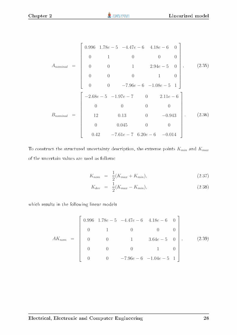
Chapter 2 Linearized modelAnominal =
0.996 1.78e − 5 −4.47e − 6 4.18e − 6 0
0 1 0 0 0
0 0 1 2.94e − 5 0
0 0 0 1 0
0 0 −7.96e − 6 −1.08e − 5 1
, (2.35)Bnominal =
−2.68e − 5 −1.97e − 7 0 2.11e − 6
0 0 0 0
12 0.13 0 −0.943
0 0.045 0 0
0.42 −7.61e − 7 6.20e − 6 −0.014
. (2.36)To onstru t the stru tured un ertainty des ription, the extreme points Kmin and Kmaxof the un ertain values are used as follows:
Knom =1
2(Kmax + Kmin), (2.37)
Kdev =1
2(Kmax − Kmin), (2.38)whi h results in the following linear models
AKnom =
0.996 1.78e − 5 −4.47e − 6 4.18e − 6 0
0 1 0 0 0
0 0 1 3.64e − 5 0
0 0 0 1 0
0 0 −7.96e − 6 −1.04e − 5 1
, (2.39)
Ele tri al, Ele troni and Computer Engineering 28

Chapter 2 Linearized modelAKdev =
0 0 0 0 0
0 0 0 0 0
0 0 0 3.08e − 5 0
0 0 0 0 0
0 0 3.22e − 6 4.82e − 6 0
, (2.40)BKnom =
−2.68e − 5 −1.97e − 7 0 2.11e − 6
0 0 0 0
12 0.13 0 −1.17
0 0.045 0 0
0.41 −7.46e − 7 6.08e − 6 −0.017
, (2.41)BKdev =
0 0 0 2.21e6
0 0 0 0
0 0 0 0.988
0 0 0 0
0.11 2.92e − 7 3.03e − 6 0.014
, (2.42)where AKdev ≡ BpCq and BKdev ≡ BpDqu.2.4.4 Linear models analysisThe linear models are ompared to the nonlinear model in order to as ertain whetherthey approximate the nonlinear model su iently well. Three s enarios are used; thenominal ase; parameters that produ e the least e ien y, and parameters that produ ethe best e ien y, i.e. the lower and upper bounds respe tively as given in table 2.3. Theparameters inuen e the dynami s of the model and ause deviation from the nominal ase. Only the extreme ases are do umented here, be ause they would provide thelargest deviation from the nominal ase. In all ases, the inputs are rst set to theirmaximum levels, and then to their minimum levels. All these simulations (gures 2.3, 2.4and 2.5) show that the linear models approximate the nonlinear model very well. Theworst approximation is for arbon, whi h shows the most nonlinear response of all theEle tri al, Ele troni and Computer Engineering 29

Chapter 2 Linearized modelvariables. In gure 2.6, the de arburization responses of all the dierent s enarios areshown on top of ea h other, and it is lear that only the inputs ause a slightly dierentresponse, while the parameter values have no signi ant inuen e. This result shows thatthe inputs do have a slight inuen e on de arburization, but not enough to a elerate thepro ess signi antly. The pro ess an only be a elerated if the target temperature and arbon ontent an be rea hed in a shorter time.A modal analysis (How, 2001) is done on the linearized model in order to determineif the arbon ontent is ontrollable. Before the modal analysis an be performed, the Amatrix is de omposed into its eigenve tors and eigenvalues as follow:A = TΛT−1, (2.43)where
T =
| |
v1 · · · vn
| |
, (2.44)T−1 =
− wT1 −...
− wTn −
, (2.45)and vi, i = 1, . . . , n is the right eigenve tor of eigenvalue λi, wi, i = 1, . . . , n is the lefteigenve tor of eigenvalue λi and Λ = diag(λ1, . . . , λn) is the matrix of eigenvalues. To he k the ontrollability of the arbon ontent, a modal analysis is performed as follows:
ControllabilityC = wT1 B, (2.46)
=
[
1.00 −5.70e − 3 1.45e − 3 −1.36e − 3 0
]
B, (2.47)=
[
1.74e − 2 1.28e − 4 0 −1.70e − 3
]
, (2.48)where the B matrix used in the analysis is the matrix (2.36). The ontrollability analysisEle tri al, Ele troni and Computer Engineering 30

Chapter 2 Linearized model
0 100 200 300 400 500 6001550
1600
1650
1700
1750
1800
1850
1900
1950
2000
Time (seconds)
Bat
h T
empe
ratu
re (
Cel
sius
)Bath Temperature
NonlinearLinear
0 100 200 300 400 500 6004000
5000
6000
7000
8000
9000
10000
11000
12000
Time (seconds)
FeO
(K
ilogr
am)
Amount of FeO in Slag
NonlinearLinear
0 100 200 300 400 500 6000.02
0.04
0.06
0.08
0.1
0.12
0.14
0.16
0.18
0.2
Time (seconds)
Per
cent
age
Car
bon
(%)
Percentage Carbon in Bath
NonlinearLinear
Figure 2.3: Linear and nonlinear model omparison with nominal parameters.of the arbon ontent (2.46-2.48) shows that the arbon ontent is ontrollable throughoxygen inje tion, slag additives and graphite inje tion. The modal analysis does not take onstraints on the inputs into onsideration. The onstraints on the inputs limit theee t of the inputs on the de arburization rate. This an be seen from gure 2.3 whi hshows the redu tion in arbon ontent with the inputs at their maximum and minimum.De arburization an therefore be des ribed as marginally ontrollable.2.4.5 Simpli ation of linear modelsFrom the previous se tion, it is lear that arbon is only marginally ontrollable. Studyingthe linear models more losely, it is lear that ertain states and inputs an be eliminated.The inputs that are ontrolled during the rening stage are oxygen inje tion, ele tri power and graphite inje tion. DRI and slag are not added during the rening stage andEle tri al, Ele troni and Computer Engineering 31

Chapter 2 Linearized model
0 100 200 300 400 500 6001550
1600
1650
1700
1750
1800
1850
Time (seconds)
Bat
h T
empe
ratu
re (
Cel
sius
)
Bath Temperature
NonlinearLinear
0 100 200 300 400 500 6004000
5000
6000
7000
8000
9000
10000
11000
Time (seconds)
FeO
(K
ilogr
am)
Amount of FeO in Slag
NonlinearLinear
0 100 200 300 400 500 6000.02
0.04
0.06
0.08
0.1
0.12
0.14
0.16
0.18
0.2
Time (seconds)
Per
cent
age
Car
bon
(%)
Percentage Carbon in Bath
NonlinearLinear
Figure 2.4: Linear and nonlinear model omparison with e ien ies at their minimum.
Ele tri al, Ele troni and Computer Engineering 32

Chapter 2 Linearized model
0 100 200 300 400 500 6001500
1600
1700
1800
1900
2000
2100
2200
Time (seconds)
Bat
h T
empe
ratu
re (
Cel
sius
)
Bath Temperature
NonlinearLinear
0 100 200 300 400 500 6004000
5000
6000
7000
8000
9000
10000
11000
12000
Time (seconds)
FeO
(K
ilogr
am)
Amount of FeO in Slag
NonlinearLinear
0 100 200 300 400 500 6000.02
0.04
0.06
0.08
0.1
0.12
0.14
0.16
0.18
0.2
Time (seconds)
Per
cent
age
Car
bon
(%)
Percentage Carbon in Bath
NonlinearLinear
Figure 2.5: Linear and nonlinear model omparison with e ien ies at their maximum.
0 100 200 300 400 500 6000.02
0.04
0.06
0.08
0.1
0.12
0.14
0.16
0.18
0.2
Time (seconds)
Per
cent
age
Car
bon
(%)
Percentage Carbon in Bath
NonlinearLinear
Figure 2.6: De arburization response with all parameter variations.Ele tri al, Ele troni and Computer Engineering 33

Chapter 2 Linearized model an be removed from the linear models. The important states are arbon ontent, FeO ontent in the slag as well as temperature. Si and SiO2 are impurities that need to beminimized, or steered to a desired spe i ation.From the se ond row of equation (2.41) , it is lear that there is no input that inuen esSi. The rst olumn of equation (2.39), shows that arbon has no inuen e on the otherstates. The se ond olumn shows that only Si has an inuen e on arbon. The inuen eof Si on arbon is very insigni ant. Carbon will therefore be removed from the model,for ontrol purposes, be ause it annot be signi antly ontrolled as shown in the previousse tion. Si annot be ontrolled and has no ee t on any relevant term, and an thereforealso be removed.From the fourth row of equation (2.41) , it is lear that only DRI addition inuen esSiO2. The fourth olumn of (2.39) shows that SiO2 has a very small inuen e on arbon,FeO and temperature. In ea h instan e, the ross- oupling term of SiO2 is at least 1000times smaller than the term for SiO2 itself. SiO2 an therefore be removed from themodel without signi antly ae ting the dynami s of the system.DRI only ae ts SiO2 and thus be omes redundant and an be safely removed. Thetwo remaining states in (2.49) have no un ertainty on the diagonal terms. The onlyremaining term that has signi ant un ertainty is the term that links FeO to temperature.The ross- ouple term between FeO and temperature is a 1000 times smaller than thediagonal term, and the un ertainty entry of this term is therefore left out, be ause of itsinsigni ant ontribution to temperature. The simplied linear model an then be givenas follows
Anominal−simplified =
1 0
−7.87e − 6 1
, (2.49)
Bnominal−simplified =
12 0 −1.17
0.41 6.07e − 6 −0.017
, (2.50)
Bdev−simplified =
0 0 0.988
0.11 3.03e − 6 0.014
, (2.51)Ele tri al, Ele troni and Computer Engineering 34

Chapter 2 Con lusionwhere Bdev−simplified ≡ BpDqu. Bp and Dqu an be realized from Bdev−simplified asBp =
1 0 0 0
0 1 1 1
, (2.52)
Dqu =
0 0 0.988
0.11 0 0
0 3.03e − 6 0
0 0 0.014
, (2.53)and the delta operator that is manipulated to des ribe the un ertain system is
∆ =
∆1 0 0 0
0 ∆2 0 0
0 0 ∆3 0
0 0 0 ∆4
, (2.54)where −1 ≤ ∆i ≤ 1, i = 1, 2, 3, 4.2.4.6 Analysis of simplied linear modelsThe simplied linear models are ompared to the original nonlinear model. Three s enar-ios are used; the nominal ase; parameters that produ e the least e ien y, and param-eters that produ e the best e ien y. In all ases, the inputs are set to their maximumlevels.Figure 2.7 shows that the simplied linear models approximate the nonlinear modelreasonably well. The simplied linear models are therefore taken to be suitable as theinternal model for the model predi tive ontrollers.2.5 Con lusionIn this hapter the redu ed nonlinear model for the rening stage of the ele tri ar furna e was linearized. The stru tured un ertainty des ription was used to des ribe theEle tri al, Ele troni and Computer Engineering 35

Chapter 2 Con lusion0 200 400 600
1500
1600
1700
1800
1900
2000
Time (seconds)
Bat
h T
empe
ratu
re (
Cel
sius
)Bath Temperature
NonlinearLinear(a) Nominal 0 200 400 600
1550
1600
1650
1700
1750
1800
1850
Time (seconds)
Bat
h T
empe
ratu
re (
Cel
sius
)
Bath Temperature
NonlinearLinear(b) E ien ies Minimum 0 200 400 600
1400
1600
1800
2000
2200
Time (seconds)
Bat
h T
empe
ratu
re (
Cel
sius
)
Bath Temperature
NonlinearLinear( ) E ien ies Maximum
0 200 400 6004000
6000
8000
10000
12000
Time (seconds)
FeO
Amount of FeO in slag
NonlinearLinear
(d) Nominal 0 200 400 6004000
6000
8000
10000
12000
Time (seconds)
FeO
Amount of FeO in slag
NonlinearLinear
(e) E ien ies Minimum 0 200 400 6004000
6000
8000
10000
12000
Time (seconds)
FeO
Amount of FeO in slag
NonlinearLinear
(f) E ien ies MaximumFigure 2.7: Simulation to ompare simplied linear model to nonlinear model.un ertainty of the nonlinear model in terms of linear models. A simulation study showedthat the linear models approximated the nonlinear models reasonably well. The onlyvariable that showed signi ant deviation was arbon, be ause of its highly nonlinearbehaviour.In the simpli ation of the linear models, it was shown that arbon is not signi antly ontrollable, whi h implies that ontrol annot be used to a elerate the rening stage.The best option would be to ensure that the tapping temperature is at the desired valueby the time arbon rea hes its desired level.The simplied linear models approximated the nonlinear model reasonably well withregards to FeO and temperature.The simplied linear models are used in the synthesis of the model predi tive on-trollers in hapter 3.Ele tri al, Ele troni and Computer Engineering 36

Chapter 3Model predi tive ontrolThis hapter des ribes model predi tive ontrol and espe ially robust model predi tive ontrol that is applied to the plant outlined in hapter 2. The hapter starts by explain-ing model predi tive ontrol and its history, followed by a des ription of robust modelpredi tive ontrol and the reason for its development, and nally fo uses on the ontrollertheory used for the simulation study in hapter 4. The des ription of model predi tive ontrol and the development of stability theory in luding robust stability are summarizedin the survey done by Mayne et al. (2000).3.1 Introdu tionModel predi tive ontrol (MPC), also known as re eding horizon ontrol (RHC), uses amathemati al model of a system to predi t its future behaviour in order to al ulate asequen e of ontrol moves (N steps) into the future that will optimize (usually minimize)an obje tive or penalty fun tion, whi h des ribes a measure of performan e of the system.The rst ontrol move of the al ulated sequen e is applied to the system and a new mea-surement is taken. The pro ess is then repeated for the next time step. Model predi tive ontrol al ulates the ontrol sequen e on-line at ea h time step, ompared to onventional ontrol theory where the ontrol law is pre- al ulated and valid for all possible states of thesystem. Model predi tive ontrol has the distin t advantage of ontrolling multi-variablesystems well and an expli itly take into onsideration onstraints on the inputs (su h as37

Chapter 3 Introdu tiona tuators, valves, et .) as well as states or outputs (Cama ho and Bordons, 2003). MPCis espe ially useful in situations where an expli it ontroller annot be al ulated oine.The basi ideas present in the model predi tive ontrol family a ording to Cama ho and Bordons(2003) are:• outputs at future time instan es are predi ted by the expli it use of a mathemati almodel ;• an obje tive fun tion is minimized by al ulating the appropriate ontrol sequen e;and• at ea h time instant, the horizon is displa ed towards the future, whi h involvesapplying the rst ontrol signal al ulated at ea h time instan e to the system; alled the re eding horizon strategy.The MPC theory des ribed in this hapter is in dis rete time and the system takes thefollowing form (Mayne et al., 2000):
x(k + 1) = f(x(k), u(k)), (3.1)y(k) = g(x(k)). (3.2)The ontrol and state sequen es must satisfy
x(k) ∈ X, (3.3)u(k) ∈ U, (3.4)where X ⊂ R
n and U ⊂ Rm. The obje tive fun tion that is used in the optimizationpro ess has the following form:
V (x, k,u) =k+N−1∑
i=k
l(x(i), u(i)) + F (x(k + N)), (3.5)Ele tri al, Ele troni and Computer Engineering 38

Chapter 3 Introdu tionwhere l(x(i), u(i)) is the ost at ea h time step into the future with regards to the statesand inputs, while F (x(k+N)) is the ost at the nal state rea hed after the whole ontrolsequen e has been applied. At ea h time k, the nal time is k+N, whi h in reases as kin reases and is alled a re eding horizon. In ertain model predi tive ontrol formulations,a terminal onstraint set is denedx(k + N) ∈ Xf ⊂ X. (3.6)The optimization of the obje tive fun tion is performed subje t to the onstraints onthe ontrol and state sequen es and in ertain ases the terminal onstraint to yield theoptimized ontrol sequen e
uo(x, k) = (uo(k; (x, k)), uo(k + 1; (x, k)), ..., uo(k + N − 1; (x, k))), (3.7)and optimized value for the obje tive fun tion
V o(x, k) = V (x, k,uo), (3.8)where (x, k) denotes that the urrent state is x at time k. The rst ontrol move at timek of the sequen e uo(x, k) is implemented to form an impli it ontrol law for time k
κ(x, k) = uo(k; (x, k)). (3.9)The obje tive fun tion is time invariant, be ause neither l(x(i), u(i)) nor F (x(k +N))have terms that depend on time. The optimization problem PN(x) an be dened asstarting at time 0. N represents the nite predi tion horizon over whi h the optimizationtakes pla e, and the optimization problem an be redened as
PN(x) : V oN(x) = min
u
VN(x,u)|u ∈ UN , (3.10)Ele tri al, Ele troni and Computer Engineering 39

Chapter 3 Introdu tionwhere the obje tive fun tion is nowVN(x,u) =
N−1∑
i=0
l(x(i), u(i)) + F (x(N)), (3.11)with UN the set of feasible ontrol sequen es that satisfy the ontrol, state and terminal onstraints. If problem PN(x) is solved, the optimal ontrol sequen es are obtainedu
o(x) = uo(0, x)), uo(1, x)), ..., uo(N − 1, x), (3.12)and the optimal state traje tory, if the ontrol a tions are implemented, is given byx
o(x) = xo(0, x), xo(1, x), ..., xo(N − 1, x), xo(N, x). (3.13)The optimal obje tive value isV o
N(x) = VN(x,uo). (3.14)The rst ontrol a tion is implemented, leading to the impli it time invariant ontrol lawκN(x) = uo(0, x). (3.15)
Dynami programming an be used to determine a sequen e of obje tive fun tionsVj(·) deterministi ally in order to al ulate the sequen e of ontrol laws κj(·) oine,where j is the time-to-go until the predi tion horizon. This is possible be ause of thedeterministi nature of the open-loop optimization. This would be preferable, but isusually not possible. The dieren e between MPC and dynami programming is purely amatter of implementation. MPC diers from onventional optimal ontrol theory in thatMPC uses a re eding horizon ontrol law κN(·) rather than an innite horizon ontrollaw.Ele tri al, Ele troni and Computer Engineering 40

Chapter 3 Histori al ba kground3.2 Histori al ba kgroundModel predi tive ontrol builds on optimal ontrol theory, the theory (ne essary andsu ient onditions) of optimality, Lyapunov stability of the optimal ontrolled system,and algorithms for al ulating the optimal feedba k ontroller (if possible) (Mayne et al.,2000). There are a few important ideas in optimal ontrol that underlie MPC. The rstlinks together two prin iples of the ontrol theory developed in the 1960s: Hamilton-Ja obi-Bellman theory (Dynami Programming) and the maximum prin iple, whi h pro-vides ne essary onditions for optimality. Dynami programming provides su ient on-ditions for optimality as well as a pro edure to synthesise an optimal feedba k ontrolleru = κ(x). The maximum prin iple provides ne essary onditions of optimality as wellas omputational algorithms for determining the optimal open-loop ontrol uo(·; x) for agiven initial state x. These two prin iples are linked together as
κ(x) = uo(0; x), (3.16)in order for the optimal feedba k ontroller to be obtained by al ulating the open-loop ontrol problem for ea h x (Mayne et al., 2000). From the ommen ement of optimal ontrol theory it is stated by Lee and Markus (1967, p. 423): One te hnique for obtaininga feedba k ontroller synthesis from knowledge of open-loop ontrollers is to measure the urrent ontrol pro ess state and then ompute very rapidly for the open-loop ontrolfun tion. The rst portion of this fun tion is then used during a short time interval,after whi h a new measurement of the pro ess state is made and a new open-loop ontrolfun tion is omputed for this new measurement. The pro edure is then repeated.Kalman, as dis ussed inMayne et al. (2000), observed that optimality does not guar-antee stability. There are onditions under whi h optimality results in stability: innitehorizon ontrollers are stabilizing, if the system is stabilizable and dete table. Cal ulatinginnite horizon optimal solutions is not always pra ti al on-line and an alternate solutionwas needed to stabilize the re eding horizon ontroller. The rst results for stabilizingre eding horizon ontrollers were given by (Kleinman, 1970), who developed a minimumEle tri al, Ele troni and Computer Engineering 41

Chapter 3 Histori al ba kgroundenergy ontroller for linear systems. He showed that the feedba k ontroller is linear,time invariant and stable if a Lyapunov fun tion V (x) = xT Px is used as the obje tivefun tion. Another approa h is to dene a stability onstraint as part of the optimal on-trol problem. The stability onstraint is dened as an equality onstraint x(T ) = 0 thatfor es the solution to onverge to the origin. Thomas, as dis ussed in Mayne et al. (2000),suggested this te hnique as part of a linear quadrati ontrol problem and implementedit by using M := P−1 in pla e of P as the Ri atti variable and solving the Ri atti-likedierential equation with terminal ondition M(T ) = 0.MPC was really driven by industry as part of pro ess ontrol theory. Ri halet et al.(1978) was the rst to propose MPC for pro ess ontrol appli ations, but MPC was pro-posed earlier by Propoi and Lee and Markus (as dis ussed in Mayne et al. (2000)). TheMPCmethod, alled identi ation and ommand (IDCOM), was proposed by Ri halet et al.(1978). It uses a linear model in the form of a nite horizon impulse response, quadrati ost and onstraints on the inputs and outputs. The method makes provision for linearestimation using least squares and the algorithm for solving the open-loop optimal ontrolproblem is the dual of the identi ation algorithm.Dynami matrix ontrol (DMC) is a later method proposed by Cutler and Ramaker(1980) and Prett and Gillette (as dis ussed in Mayne et al. (2000)). DMC uses a stepresponse model, but as in IDCOM, handled onstraints in an ad-ho fashion. This lim-itation was addressed by Gar ía and Morshedi (as dis ussed in Mayne et al. (2000)) byusing quadrati programming to solve the onstrained open-loop optimization problem.This method also allows ertain violations of the onstraints in order to enlarge the setof feasible states. This method is alled QDMC (Quadrati Dynami Matrix Control).The third generation of MPC te hnology, introdu ed about a de ade ago, distin-guishes between several levels of onstraints (hard, soft and ranked). This te hnologyprovides some me hanism to re over from an infeasible solution, and addresses the issuesresulting from a ontrol stru ture that hanges in real time, and allows for a wider rangeof pro ess dynami s and ontroller spe i ations (Qin and Badgwell, 2003). The Shellmulti-variable optimizing ontrol (SMOC) uses state-spa e models, in orporates generalEle tri al, Ele troni and Computer Engineering 42

Chapter 3 Stability of MPCdisturban e models and allows for state estimation using Kalman lters (as dis ussed inMayne et al. (2000)).An independent but similar approa h was developed from the adaptive ontrol the-ory and is alled generalized predi tive ontrol (GPC). The method uses models in theba kward shift operator q-1 whi h is more general than the impulse and step responsemodels of DMC. GPC started as minimum varian e ontrol (Mayne et al., 2000) that onlyallowed for a horizon of length 1. Minimum varian e ontrol was extended to allow forlonger predi tion horizons by Peterka (1984) as well as Clarke et al. (1987a,b). GPC, andearly versions of DMC, did not expli itly in orporate stability in the method and had torely on the tuning of the predi tion horizon as well as the weights on the states and inputsto a hieve stability.3.3 Stability of MPCThe inability of both GPC and DMC to guarantee stability aused resear hers to fo usmore on modifying PN (x) to ensure stability due to in reased riti ism (Bitmead et al.,1990) of the makeshift approa h of using tuning to attain stability.With terminal equality onstraints, the system is for ed to the origin by the ontrollerthat takes the form F (x) = 0, as there is no terminal ost and the terminal set is Xf = 0.Keerthi and Gilbert, as dis ussed in Mayne et al. (2000), proposed this stabilizing strategyfor onstrained, nonlinear, dis rete systems, and showed a stability analysis of this version(terminal equality onstraints) of dis rete-time re eding horizon ontrol. MPC with aterminal equality onstraint an be used to stabilize a system that annot be stabilized by ontinuous feedba k ontrollers, a ording to Meadows et al. (as dis ussed in Mayne et al.(2000)).Using a terminal ost fun tion is an alternative approa h to ensure stability. Herethe terminal ost is F (·), but there is no terminal onstraint and the terminal set isthus Xf = Rn. For un onstrained linear systems the terminal ost of F (x) = 1
2xT Pfx isproposed by Bitmead et al. (1990).Terminal onstraint sets dier from the terminal equality onstraints, in that subsetsEle tri al, Ele troni and Computer Engineering 43

Chapter 3 Stability of MPCof Rn that in lude a neighbourhood of the origin are used to stabilize the ontrol, notjust the origin. The terminal onstraint set, as with the terminal equality onstraint,does not employ a terminal ost, thus F (x) = 0. The MPC ontroller should steer thesystem to Xf within a nite time, after whi h a lo al stabilizing ontroller κf (·) is em-ployed. This methodology is usually referred to as dual mode ontrol and was proposed byMi halska and Mayne (1993) in the ontext of onstrained, nonlinear, ontinuous systemsby using a variable horizon N.A terminal ost and onstraint set is employed in most modern model predi tive on-trollers. If a innite horizon obje tive fun tion an be used, on-line optimization is notne essary and stability and robustness an be guaranteed. In pra ti al systems, on-straints and other nonlinearities make the use of innite horizons impossible, but it ispossible to approximate an innite horizon obje tive fun tion if the system is suitably lose to the origin. By hoosing the terminal set Xf as a suitable subset of R
n, theterminal ost F (·) an be hosen to approximate an innite horizon obje tive fun tion.A terminal ost and onstraint set ontroller therefore needs a terminal onstraint setXf in whi h the terminal ost F (·) and innite horizon feedba k ontroller Kf are em-ployed. To synthesise these, Sznaier and Damborg (as dis ussed in Mayne et al. (2000))proposed that the terminal ost F (·) and feedba k ontroller Kf of a standard LQ prob-lem be used, whi h is an un onstrained innite horizon problem, when the system islinear (f(x, u) = Ax + Bu) and the state and input onstraint sets, X and U, are poly-topes. The terminal onstraint set Xf is hosen to be the maximal output admissible set(Gilbert and Tan, 1991) of the system f(x, u) = (A + BKf)x.3.3.1 Stability onditions for model predi tive ontrollersFrom the above dis ussion, it is lear that the additions of a terminal onstraint set Xf ,terminal ost F (·) and lo al feedba k ontroller κf in the terminal onstraint set, form thebasis of stabilizing model predi tive ontrol. Some onditions, in the form of axioms, areformulated (Mayne et al., 2000) for the terminal onstraint set, terminal ost and lo alfeedba k ontroller, whi h ensure that the ontroller is stabilizing.Ele tri al, Ele troni and Computer Engineering 44

Chapter 3 Stability of MPCTwo related methods are available for establishing stability. Both methods use aLyapunov fun tion as the obje tive fun tion. The rst method ensures that the obje tivefun tion V oN(x) evolves with the state from x to x+ = f(x, κN(x)) so that
V oN(x+) − V o
N (x) + l(x, κN (x)) ≤ 0, (3.17)while the alternative method uses the fa t thatV o
N(x+) − V oN(x) + l(x, κN (x)) = V o
N(x+) − VN−1(x+), (3.18)and shows that the right-hand side is negative, either dire tly or by showing that V o
1 (·) ≤
V o0 (·) and exploiting monotoni ity whi h implies that if V o
1 (·) ≤ V o0 (·) then V o
i+1(·) ≤ V oi (·)for all i ≥ 0.Assume a model predi tive ontroller that an steer the system state x to the ter-minal onstraint set Xf within the predi tion horizon N or fewer steps. The ontrolsequen e that a omplishes this is alled an admissible or feasible ontrol sequen e u =
u(0), u(1), ..., u(N − 1). This ontrol sequen e should satisfy the ontrol onstraintsu(i) ∈ U for i = 0, 1, ..., N − 1 and ensure that the ontrolled states satisfy the state onstraints xu(i) ∈ X for i = 0, 1, .., N and the nal state satises the terminal on-straint set xu(N) ∈ Xf . If the ontrol problem PN(x) is solved, the ontrol sequen eu
o(x) is obtained that will steer the system within the set of states that is possiblewith a model predi tive ontrol of horizon N, x ∈ XN . The optimal ontrol sequen eu
o(x) = u(0; x), u(1; x), ..., u(N −1; x) will result in the optimal state sequen e xo(x) =
xo(0; x), xo(1; x), ..., xo(N − 1; x), xo(N ; x). The rst ontrol a tion of uo(x), that is
u = κN (x) = uo(0; x) is implemented to get to the next state x+ = f(x, κN(x)) = xo(1; x).A feasible ontrol sequen e x(x+) for the state x+, will result in an upper bound for theoptimal obje tive fun tion V oN(x+), be ause a feasible ontrol sequen e should give a largervalue for the obje tive fun tion than an optimal ontrol sequen e. The abbreviated on-trol sequen e u(1; x), u(2; x), ..., u(N − 1; x) derived from u
o(x) should be a feasible ontrol sequen e to steer state x+ to xo(N ; x) ∈ Xf . If an extra term is added to theEle tri al, Ele troni and Computer Engineering 45

Chapter 3 Stability of MPC ontrol sequen e u(1; x), u(2; x), ..., u(N − 1; x), u, the ontrol sequen e will be feasiblefor PN(x+) if u ∈ U and u steers xo(N ; x) ∈ Xf to f(xo(N ; x), u) ∈ Xf . This will betrue if u = κf(xo(N ; x)), with the terminal state onstraint Xf and lo al ontroller κf (·)having the properties:
Xf ⊂ X, κf (x) ∈ U and f(x, κf(x)) ∈ Xf ∀x ∈ Xf , (3.19)implying that the terminal set Xf is invariant when the ontroller is κf(·). The feasible ontrol sequen e for PN(x+) isu(x) = uo(1; x), uo(2; x), ..., uo(N − 1; x), κf(x
o(N ; x)), (3.20)with the asso iated ostVN(x+, u(x)) = V o
N(x) − l(x, κN (x)) − F (xo(N ; x))
+l(xo(N ; x), κf (xo(N ; x))
+F (f(xo(N ; x), κf (xo(N ; x))). (3.21)This ost is the upper bound on V o
N (x+) and satisesVN(x+, u(x)) ≤ V o
N(x) − l(x, κN(x)), (3.22)if F (f(x, κf(x))) − F (x) + l(x, κf (x)) ≤ 0 ∀x ∈ Xf . This is a omplished if F (·) is a ontrol Lyapunov fun tion in the neighbourhood of the origin and the ontroller κf andthe terminal onstraint set Xf are hosen appropriately. If this ondition is satised, then(3.17) will hold for all x ∈ XN and it is su ient to say that the losed-loop systemx+ = f(x, κN(x)) will onverge to zero as time tends to innity, provided that the initialstate is within XN . The stability onditions an be summarized in the following axioms(Mayne et al., 2000):A1: Xf ⊂ X, Xf is a losed set and 0 ∈ Xf . This ondition implies that the stateEle tri al, Ele troni and Computer Engineering 46
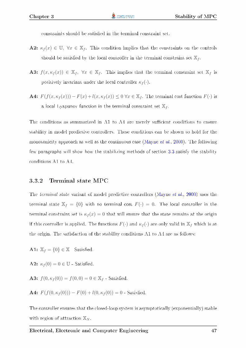
Chapter 3 Stability of MPC onstraints should be satised in the terminal onstraint set.A2: κf (x) ∈ U, ∀x ∈ Xf . This ondition implies that the onstraints on the ontrolsshould be satised by the lo al ontroller in the terminal onstraint set Xf .A3: f(x, κf(x)) ∈ Xf , ∀x ∈ Xf . This implies that the terminal onstraint set Xf ispositively invariant under the lo al ontroller κf(·).A4: F (f(x, κf(x)))−F (x) + l(x, κf (x)) ≤ 0 ∀x ∈ Xf . The terminal ost fun tion F (·) isa lo al Lyapunov fun tion in the terminal onstraint set Xf .The onditions as summarized in A1 to A4 are merely su ient onditions to ensurestability in model predi tive ontrollers. These onditions an be shown to hold for themonotoni ity approa h as well as the ontinuous ase (Mayne et al., 2000). The followingfew paragraphs will show how the stabilizing methods of se tion 3.3 satisfy the stability onditions A1 to A4.3.3.2 Terminal state MPCThe terminal state variant of model predi tive ontrollers (Mayne et al., 2000) uses theterminal state Xf = 0 with no terminal ost F (·) = 0. The lo al ontroller in theterminal onstraint set is κf(x) = 0 that will ensure that the state remains at the originif this ontroller is applied. The fun tions F (·) and κf(·) are only valid in Xf whi h is atthe origin. The satisfa tion of the stability onditions A1 to A4 are as follows:A1: Xf = 0 ∈ X - Satised.A2: κf (0) = 0 ∈ U - Satised.A3: f(0, κf(0)) = f(0, 0) = 0 ∈ Xf - Satised.A4: F (f(0, κf(0))) − F (0) + l(0, κf(0)) = 0 - Satised.The ontroller ensures that the losed-loop system is asymptoti ally (exponentially) stablewith region of attra tion XN .Ele tri al, Ele troni and Computer Engineering 47

Chapter 3 Stability of MPC3.3.3 Terminal ost MPCTerminal ost model predi tive ontrollers are only valid for linear un onstrained (Bitmead et al.,1990) and linear, stable, onstrained (Rawlings and Muske, 1993) ases. In order to en-sure stability a terminal onstraint is ne essary if the system is nonlinear or linear, on-strained and unstable. Linear, un onstrained systems are dened as f(x, u) = Ax + Bu,and l(x, u) = 12(|x|2Q + |u|2R) where Q > 0 and R > 0. The rst three onditions A1 to A3are trivially satised in the un onstrained ase, be ause X = R
n and U = Rm. In the asewhere A and B are stabilizable, the lo al ontroller is dened as κf := Kfx, and Pf > 0should satisfy the Lyapunov equation
ATf PAf + Qf = 0, Af := A + BKf , Qf := Q + KfRKf , (3.23)then the terminal ost fun tion F (x) := 1
2xT Pfx satises A4 and the losed-loop system isasymptoti ally (exponentially) stable with a region of attra tion R
n. Linear, onstrained,stable systems have ontrol onstraints u ∈ U, but no onstraints on the states, thusX = Xf = R
n. In order to satisfy A2, the ontroller fun tion, if linear, should beκf(x) = 0 (Rawlings and Muske, 1993), that leads to the rst three onditions (A1 toA3) being satised. The nal ondition A4 is satised if the terminal ost fun tion isF (x) := 1
2xT Pfx, where Pf satisfy the Lyapunov equation AT PA + Q = 0, that results ina ontroller with asymptoti (exponential) stability with region of attra tion R
n.3.3.4 Terminal onstraint set MPCTerminal onstraint set model predi tive ontrollers employ a terminal onstraint setx(N) ∈ Xf without a terminal ost F (x) = 0 for nonlinear, onstrained systems. Mi halska and Mayne(1993) introdu ed the idea of a variable predi tion horizon N for ontinuous-time, on-strained, nonlinear systems. S okaert et al. (1999) proposed a xed horizon version fornonlinear, onstrained, dis rete-time systems. The ontroller steers the state of the sys-tem x to within the terminal onstraint set Xf , after whi h a lo al stabilizing ontrollerκf(x) = Kfx is employed. This type of MPC is sometimes referred to as dual-mode MPC.Ele tri al, Ele troni and Computer Engineering 48

Chapter 3 Stability of MPCThis method is similar to the terminal equality onstraint method, ex ept that the equal-ity 0 is repla ed by a set Xf . The lo al ontroller κf (·) and the terminal onstraint setXf are hosen to satisfy the rst three onditions A1 to A3. The lo al ontroller κf (·) is hosen to steer the system exponentially fast to the origin for all states in the terminal onstraint set (∀x ∈ Xf). The stage ost of the obje tive fun tion l(x, κf(x)) should be 0when the system state is within the terminal onstraint set Xf in order to satisfy A4. Asuitable hoi e for the stage ost is
l(x, u) := α(x)l(x, u), (3.24)where α(x) = 1, ∀x /∈ Xf , else α(x) = 0 and l(x, u) = 12(xT Qx + uTRu), where Q > 0and R > 0. The losed-loop system is exponentially stable with domain of attra tion XN ,be ause the MPC ontroller steers the system with initial state x ∈ XN within nite timeto Xf with the ontroller value κN(·).
3.3.5 Terminal ost and onstraint set MPCTerminal ost and onstraint sets are employed by most modern model predi tive on-trollers. In linear, onstrained systems the terminal ost fun tion an be hosen F (x) =
V 0uc(x) = 1
2xT Pfx, that is the same as the un onstrained innite horizon optimal on-trol problem. The lo al ontroller κf (x) = Kfx is the optimal innite horizon on-troller and the terminal onstraint set Xf is the maximal admissible set for the system
x+ = Afx, Af := A + BKf , thus satisfying A1-A4. This results in an exponentiallystable ontroller with domain of attra tion Xf . The ideal hoi e for the terminal ostwould be to hoose F (x) = V o∞(x), the obje tive fun tion of an innite horizon optimal ontroller, that would result in the obje tive fun tion for model predi tive ontroller being
V oN(x) = V o
∞(x), and on-line optimization would not be ne essary. The resulting MPC ontroller will have all the advantages of innite horizon ontrol. This is usually notpra ti al, and the use of the terminal onstraint set Xf and F (x) = V 0uc(x) = 1
2xT Pfxapproximates the advantages of using F (x) = V o
∞(x). The nonlinear ase is also given inEle tri al, Ele troni and Computer Engineering 49

Chapter 3 Robust MPC - Stability of un ertain systemsMayne et al. (2000).From this dis ussion, it is lear that the use of a terminal onstraint set Xf , terminal ost fun tion F (·) and lo al stabilizing ontroller κf(·) is ne essary to ensure stabilityin model predi tive ontrol. The rst two requirements, terminal onstraint set Xf andterminal ost fun tion F (·), are expli itly in orporated into the ontroller, while the feed-ba k ontroller κf(·) is only impli itly needed to prove stability. If the ost fun tion F (·)is as lose to the obje tive fun tion V o∞(·) as possible, the losed-loop traje tory is exa tlythe same as that predi ted by the solution of the optimal ontrol problem PN(x).3.4 Robust MPC - Stability of un ertain systemsRobust model predi tive ontrol is on erned with the stability and performan e of the losed-loop system in the presen e of un ertainty in the plant model. Early studies inrobustness of model predi tive ontrollers onsidered un onstrained systems and foundthat if the Lyapunov fun tion retains its des ent property in the presen e of disturban es(un ertainty), it will remain stable. In the onstrained ase, the problem be omes more omplex, be ause the un ertainty or disturban es should not ause the losed-loop systemto violate its state or ontrol onstraints.Ri halet et al. (1978) performed one the earliest studies in robustness on systems withimpulse response models, by investigating the ee t of gain mismat hes on the losed-loopsystem. Later work on systems modelled by impulse responses approa hed the optimal ontrol problem as a min-max problem, that aused the problem to grow exponentiallywith the size of the predi tion horizon.There are several approa hes to robust model predi tive ontrol, the rst being a studyof the robustness of model predi tive ontrol designed with a nominal model (that does nottake un ertainty into a ount). The se ond approa h onsiders all the possible realizationsof the un ertain system when al ulating the open-loop optimal ontroller (min-max open-loop MPC). The open-loop nature of model predi tive ontrol is a problem when modelun ertainty is present and the third approa h addresses this by introdu ing feedba k inthe optimal ontrol problem that is solved on-line.Ele tri al, Ele troni and Computer Engineering 50

Chapter 3 Robust MPC - Stability of un ertain systemsFor the dis ussion of robust model predi tive ontrol, the un ertain system is des ribedasx+ = f(x, u, w), (3.25)y = g(x), (3.26)where the state x and ontrol u satisfy the same onstraints
x(k) ∈ X, (3.27)u(k) ∈ U, (3.28)and the disturban e or un ertainty w satises w ∈ W (x(k), u(k)) for all k where, for ea h
(x, u), W (x, u) is losed and ontains the origin in its interior. The disturban e sequen ew := w(0), w(1), ..., w(N − 1) together with the ontrol sequen e u and initial statex will produ e the resulting state traje tory xu,w(·; x). Let F(x, u) := f(x, u, W (x, u)),whi h will map values in X and U to subsets of R
n, resulting in x+ ∈ F(x, u).De Ni olao et al. (1996) and Magni and Sepul hre (1997) studied the inherent robust-ness of model predi tive ontrollers that were designed without taking un ertainty intoa ount.3.4.1 Stability onditions for robust MPCMost versions of robust model predi tive ontrol take all the realizations of the un ertaintyor disturban e w into onsideration that requires strengthened assumptions to be satised,whi h are summarized as robust versions of axioms A1-A4 (Mayne et al., 2000):A1: Xf ⊂ X, Xf losed, 0 ∈ Xf .A2: κf (x) ∈ U, ∀x ∈ Xf .A3a: f(x, κf(x), w) ∈ Xf , ∀x ∈ Xf , ∀w ∈ W (x, κf (x)).A4a: F (f(x, κf(x), w)) − F (x) + l(x, κf (x), w) ≤ 0, ∀x ∈ Xf , ∀w ∈ W (x, κf(x)).Ele tri al, Ele troni and Computer Engineering 51

Chapter 3 Robust MPC - Stability of un ertain systemsIf F (·) is a robust Lyapunov fun tion in the neighbourhood of the origin, there exists atriple (F (·), Xf , κf (·)), whi h ensures that A4a is satised and results in an asymptoti allyor exponentially stable ontroller.3.4.2 Open-loop min-max MPCOpen-loop min-max model predi tive ontrol onsiders all the possible realizations of theun ertain system in order to ensure that the state, ontrol and terminal onstraints aremet for all the possible realizations (Mi halska and Mayne, 1993). The obje tive fun tionvalue in this ase is determined for ea h realization
J(x,u,w) :=N−1∑
i=0
l(x(i), u(i)) + F (x(N)), (3.29)where x(i) = xu,w(i; x; 0) and the nal obje tive value is the worst ase for all the real-izationsVN (x,u) := maxJ(x,u,w)|w ∈ WN(x,u), (3.30)where WN (x,u) is the set of admissible disturban e sequen es. Other hoi es are to takethe obje tive value as the nominal obje tive value by using w = 0. Badgwell (as dis ussedin Mayne et al. (2000)) used an interesting approa h, where the ontroller should redu ethe obje tive fun tion value for every realization, whi h is assumed nite, for a linearsystem. This is stronger than only redu ing the worst- ase obje tive value.The set of admissible ontrol sequen es Uol
N (x) is that set whi h satises the ontrol,state and terminal onstraints for all possible realization of the disturban e sequen e wwhen the initial state is x. Suppose the the set Xoli , for all i ≥ 0, is the set of statesthat an be robustly steered to the terminal state onstraint Xf in i steps or less by anadmissible ontrol sequen e u ∈ Uol
N (x). The open-loop optimal ontrol problem isP ol
N (x) : V oN(x) = minVN(x,u)|u ∈ Uol
N (x). (3.31)Ele tri al, Ele troni and Computer Engineering 52

Chapter 3 Robust MPC - Stability of un ertain systemsThe solution to P olN (x) yields the optimal ontrol sequen e u
o(x), where the impli it min-max ontrol law isκol
N(x) := uo(0; x), (3.32)as in the nominal ase. The ontrol sequen e will result in a bundle of optimal statesequen es xo(x,w) as a result of the disturban e sequen es w, so that
xo(x,u) = xo(0; x;w), xo(1; x;w), ..., xo(N − 1; x;w), xo(N ; x;w). (3.33)The triple (F (·), Xf , κf (·)) is assumed to satisfy the stability onditions A1-A4a. Assumethe pro ess is started with an initial state x ∈ X ol
N and has an optimal (and by impli ationa feasible) ontrol sequen e uo(0; x), uo(1; x), ..., uo(N − 1; x) for the optimal ontrolproblem P olN (x) that steers the state to within the terminal onstraint set Xf within N stepsor less, so that xo(N ; x;w) ∈ Xf , ∀w ∈ W(x,uo(x)). As a result the abbreviated ontrolsequen e uo(1; x), uo(2; x), ..., uo(N − 1; x) should steer the state x+ ∈ F(x, κN(x)) tothe terminal onstraint set Xf within N − 1 steps or less, where x+ ∈ X ol
N−1. A problemarises when a feasible ontrol sequen e needs to be generated by adding a term to theabbreviated ontrol sequen eu(x) = uo(1; x), uo(2; x), ..., uo(N − 1; x), v, (3.34)for the optimal ontrol problem P ol
N (x+), where the ontrol a tion v ∈ U is required tosatisfy f(xo(N ; x;w), v, wN) ∈ XN for all w ∈ W(x,uo(x)). The stability ondition A3adoes not ensure that su h a ontrol a tion v an be obtained, whi h prevents the upperbound of the obje tive fun tion V oN (x+) from being al ulated. Mi halska and Mayne(1993) ir umvent this problem by using a variable horizon optimal ontrol problem P (x)with de ision variables (u, N). The optimal solution (uo(x); No(x)) is obtained by solving
Ele tri al, Ele troni and Computer Engineering 53

Chapter 3 Robust MPC - Stability of un ertain systemsthe optimal ontrol problem P (x), whereu
o(x) = uo(0; x), uo(1; x), ..., uo(N(x) − 1; x).For the optimal ontrol problem P (x+) the solution (u(x), No(x)−1) is a feasible solutionfor any x+ ∈ X (x, κN(x)). The variable horizon obje tive fun tion V o(·) and impli it ontroller κol(·) will ensure that stability ondition A4a holds for all x ∈ XolN ⊂ Xf , ∀w ∈
W (x, κol(x)). Inside the terminal onstraint set Xf , a suitable lo al ontroller κf(·) is usedsubje t to stability onditions A1-A4a. This will result in an asymptoti (exponential)stable ontroller with domain of attra tion XolN , subje t to further modest assumptions(Mi halska and Mayne, 1993).
3.4.3 Feedba k robust MPCFeedba k robust model predi tive ontrol is better suited for un ertain systems than open-loop min-max ontrollers, be ause open-loop ontrollers assume that the traje tories ofthe system may diverge, whi h may ause XolN to be very small, or even empty for amodest sized predi tion horizon N , whi h is very onservative. This happens be ausethe open-loop min-max ontrollers do not take the ee t of feedba k into onsideration,whi h would prevent the traje tories from diverging too mu h. To address the short om-ings of open-loop min-max ontrol, feedba k MPC was proposed by Lee and Yu (1997),S okaert and Mayne (1998), Magni et al. (2001) and Kothare et al. (1996). In feedba kmodel predi tive ontrol, the ontrol sequen e u is repla ed by a ontrol poli y π whi his a sequen e of ontrol laws:
π := u(o), κ1(·), ..., κN−1(·), (3.35)where κi(·) : X → U is a ontrol law for ea h i, while u(0) is a ontrol a tion, be ausethere is only one initial state. The obje tive fun tion for the feedba k model predi tiveEle tri al, Ele troni and Computer Engineering 54

Chapter 3 Robust MPC - Stability of un ertain systems ontroller isVN(x, π) := maxJ(x, π,w)|w ∈ WN(x, π) (3.36)and the obje tive fun tion for ea h realizationJ(x, π,w) :=
N−1∑
i=0
l(x(i), u(i)) + F (x(N)), (3.37)where x(i) = xπ,u(i; x) is the state at time i resulting from an initial state at time 0,a ontrol poli y π and a disturban e sequen e w. The admissible set of disturban es,given the ontrol poli y π is implemented, is WN (x, π). The set of admissible ontrolpoli ies that will satisfy the ontrol, state and terminal onstraints for all the admissibledisturban es with initial state x, is ΠN (x). The set of initial states that an be steeredto the terminal onstraint set Xf by an admissible ontrol poli y π in i steps or less, isX
fbi , ∀i ≥ 0. The feedba k optimal ontrol problem be omes
P fbN (x) : V o
N(x) = minVN(x, π)|π ∈ ΠN(x). (3.38)If a solution to P fbN (x) exists, the optimal ontrol poli y is
πo(x) = uo(0; x), κo1(·; x), κo
2(·; x), ..., κoN−1(·; x), (3.39)where the impli it feedba k model predi tive ontrol law is
κfbN (x) := uo(0; x). (3.40)If the stability onditions A1-A4a are satised for P fb
N (x), a feasible ontrol poli y forP fb
N (x+) for all x+ ∈ F(x, κfbN (x)) and x ∈ X
fbN is
π(x, x+) := κo1(x
+; x), κo2(·; x), ..., κN−1(·; x), κf(·). (3.41)
Ele tri al, Ele troni and Computer Engineering 55

Chapter 3 Robust MPC - Stability of un ertain systemsWith this feasible ontrol poli y, and with XfbN an invariant set for x+ ∈ F(x, κfb
N (x)),assumption A4a will be satised for all x ∈ XfbN and w ∈ W (x, κfb
N (x)). The resultingrobust model predi tive ontroller is asymptoti ally (exponentially) stable with domainof attra tion XfbN under further modest assumptions. The results are very similar to open-loop min-max ontrol, ex ept that the domain of attra tion X
fbN in ludes X
olN and ouldpossibly be mu h larger. Feedba k MPC is en ouraging, but suers from mu h higher omplexity than open-loop min-max ontrol.3.4.4 Robust MPC implementationsSome implementations of robust model predi tive ontrollers that fall into the above-mentioned ategories, are linear matrix inequality (LMI) based ontrollers that produ efeedba k poli ies whi h are implemented at ea h time interval. The problem with these ontrollers is that they use an ellipsoid invariant set for their domain of attra tion, whi hmakes them onservative. This is be ause the sets must be symmetri , and in systemswhere the onstraints are non-symmetri , the ellipsoid sets will be a small subset ofthe maximum admissible set. The feedba k robust MPC te hnique was introdu ed byKothare et al. (1996). The te hnique was improved by Cuzzola et al. (2002) by des ribingthe un ertain system as a polytope and applying dierent Lyapunov fun tions to ea hvertex of the un ertain polytope to redu e the onservatism of the method. The methoduses semidenite programming (SDP) to solve the minimization problem on-line, whi his omputationally very expensive ompared to quadrati programming (QP) used innominal MPC. Further improvements made by Wan and Kothare (2003); Casavolaa et al.(2004); Ding et al. (2004) resulted in an attempt to move as mu h of the al ulation aspossible oine. The LMI methods have been used to robustify PID (Proportional, Integraland Derivative) ontrol (Ge et al., 2002) and a few ase studies on LMI based ontrol weredone by Park and Rhee (2001) and Wu (2001).An approa h to feedba k robust model predi tive ontrol is proposed by Langson et al.(2004) who uses tubes to en apsulate all the possible states that an result from the ontroller. If the un ertainties an be su iently des ribed, the optimization problemEle tri al, Ele troni and Computer Engineering 56

Chapter 3 Robust MPC - Stability of un ertain systemsneeds only be al ulated on e, and the ontrol poli y will steer the system to the terminal onstraint set Xf , where a lo al stabilizing ontroller will keep the un ertain system inthe terminal onstraint set.There is a movement in robust model predi tive ontrol to redu e the on-line ompu-tational burden. Lee and Kouvaritakis (2002) propose a method where optimal ontrolsequen es are omputed oine for ertain anoni al states. A feasible (suboptimal) on-trol sequen e is generated on-line for the state x by using linear ombinations of thepre omputed optimal ontrol sequen es. The on-line omputation is redu ed to a simplematrix multipli ation, and no on-line optimization is performed. De la Pena et al. (2004)proposed using multi-parametri methods to des ribe a suboptimal ontrol strategy thatwill be less omputationally expensive for on-line use. Fukushima and Bitmead (2005)in orporate the un ertainties and bounded disturban es into a omparison model, andthe ontrol algorithm an then be set up as a nominal MPC (without un ertainties) withonly a QP problem to solve on-line. The omparison model provides an upper bound onthe obje tive fun tion value used in the on-line optimization. Mayne et al. (2005) redu edthe on-line optimization of robust model predi tive ontrol to a QP problem, with theinitial state as well as the ontrol sequen e as part of the de ision variables. As the on-lineproblem is a nominal ontrol problem, tighter onstraints are used to ensure robustness.This is only valid for linear systems, and annot be easily extended to nonlinear systems.An interesting robust ontroller, in a pro ess ontrol environment, was proposed byTsai et al. (2002), whi h uses neural adaptive ontrol based on arti ial neural networks(ANN) in onjun tion with normal robust MPC. The outputs of the two ontrollers are ombined and the weightings are al ulated from regional knowledge of the ANN, whi hdetermines whether the ANN is operating in an area of good predi tion hara teristi s ornot.An alternative approa h to robust model predi tive ontrol, is to modify the obje tivefun tion to ensure robust stability in the presen e of un ertainties. Wang and Romagnoli(2003) used robust identi ation theory to onstru t a generalized obje tive fun tion, torepla e the quadrati obje tive fun tion usually employed to produ e a robust ontroller.Ele tri al, Ele troni and Computer Engineering 57

Chapter 3 Robust model predi tive ontrollersThe on-line optimization uses the nominal model, and robustness is provided by theobje tive fun tion. A method for robustifying generalized predi tive ontrol (GPC) hasbeen proposed by Rodríguez and Dumur (2005).The robust model predi tive ontrollers do not always provide o-set free tra king,and this problem is addressed by Wang and Rawlings (2004b,a) who use a robust predi -tor that updates itself ea h time measurements are available to ensure that the o-set iseliminated. Panno hia (2004) approa hes the problem by designing a robust linear feed-ba k ontroller and an appropriate invariant set where the ontroller will satisfy the on-straints. The ontroller uses the dual-mode approa h suggested by Rossiter et al. (1998)and later implemented by Kouvaritakis et al. (2000); S huurmans and Rossiter (2000) andLee and Kouvaritakis (2000), where the feedba k law ui(·) in the poli y π is restri ted tohave the form ui(x) = vi + Kx, i = 0, 1, 2, ..., N − 1, that hanges the optimization prob-lem to al ulating the free ontrol moves v0, v1, v2, ..., vN−1 rather than the poli y. Thedual-mode ontroller remains essentially a feedba k model predi tive ontrol, be ause Kxlimits the diversion of traje tories of the losed-loop system.3.5 Robust model predi tive ontrollersIn this se tion two robust model predi tive ontroller methods, used in omparison withnominal MPC in the next hapter, are dis ussed in more detail. The rst method, pro-posed by Kothare et al. (1996) al ulates a feedba k poli y at ea h time interval forthe system. The se ond method onsists of a dual-mode ontroller rst proposed byRossiter et al. (1998), where the feedba k poli y is a ombination of an open-loop feed-ba k ontrol law κf ≡ −Kx with free ontrol moves v, ui(·) = v − Kx.3.5.1 Robust MPC using LMIsTraditional model predi tive ontrol solves an open-loop onstrained optimization prob-lem. The internal model is a nominal model and the assumption is that feedba k will ompensate for the model un ertainty and unmeasured disturban es. The stru ture ofEle tri al, Ele troni and Computer Engineering 58

Chapter 3 Robust model predi tive ontrollersthe value fun tion usually does not take the ee t of feedba k into onsideration.Kothare et al. (1996) formulated a new model predi tive ontrol strategy with robust-ness in mind. The robust ontroller design expli itly in orporates model un ertainty. Thevalue fun tion is also formulated to take feedba k into onsideration. The whole theory isbased on linear matrix inequalities (LMI) (Boyd et al., 1994). With urrent interior pointmethods and omputer te hnology, these fun tions an now be solved fast enough to beappli able in on-line use. Current model predi tive ontrol theory an be re ast as linearmatrix inequalities that in orporate input and output onstraints, model un ertainty androbustness measures.3.5.1.1 System des riptionsThe system is dened as a linear time-varying system by Kothare et al. (1996).
x(k + 1) = A(k)x(k) + B(k)u(k), (3.42)y(k) = Cx(k), (3.43)
[ A(k) B(k)] ∈ Ω, (3.44)where x(k) is the state of the system, u(k) is the ontrol ve tor, y(k) is the output ofthe system and Ω is the set of models that des ribes the system. For polytopi un ertainsystems, the set Ω is the polytopeΩ ∈ Co
[ A1 B1 ], [ A2 B2 ], ..., [ Ai Bi ]
,where Co denotes the onvex hull.A se ond representation of the system is alled the stru tured feedba k un ertainty. Theun ertainty is des ribed as perturbations in the feedba k loop. The system des riptionlooks as follows:Ele tri al, Ele troni and Computer Engineering 59

Chapter 3 Robust model predi tive ontrollersx(k + 1) = Ax(k) + Bu(k) + Bpp(k),
y(k) = Cx(k),
q(k) = Cpx(k) + Dquu(k), (3.45)p(k) = (∆q)(k).The operator ∆ is blo k-diagonal:∆ =
∆1
∆2
.
.
∆r
, (3.46)with ∆i : R
ni → Rni.For a linear time varying system, it an be shown that (3.45) an be ast in the formof (3.42-3.43) by using
Ω =
[
A + Bp∆Cq B + Bp∆Dqu
]
: ∆ satises (3.46) with σ(∆i) ≤ 1
.(3.47)3.5.1.2 Obje tive fun tionThe stage ost of the obje tive fun tion used is a standard quadrati fun tion of the formJp(k) =
p∑
i=0
[
x(k + i|k)T Q1x(k + i|k) + u(k + i|k)T Ru(k + i|k)]
, (3.48)where Q1 > 0 and R > 0 are symmetri weighting matri es. The obje tive fun tionstrives to drive the state ve tor to zero. The Q weighting matrix denes the severity ofthe state position penalty and the R matrix that of the ontrol a tion. The ratio of Qand R will determine the priority of state position versus ontrol a tion obje tives.Ele tri al, Ele troni and Computer Engineering 60

Chapter 3 Robust model predi tive ontrollers3.5.1.3 Linear matrix inequalitiesLinear matrix inequalities have the following formF (x) = F0 +
f∑
i=1
xiFi > 0, (3.49)where x1, x2, ..., xf are the variables, Fi = F Ti ∈ R
nxn are given, and F (x) > 0 meansthat F (x) is positive-denite. Multiple LMIs F1(x) > 0, ..., Fn(x) > 0 an be expressedas the single LMIdiag (F1(x), ..., Fn(x)) > 0. (3.50)Convex quadrati inequalities are onverted to linear form using S hur's omplements. Inthe ase of matrix inequalities of the form
R(x) > 0, Q(x) − S(x)R(x)−1S(x)T > 0, (3.51)orQ(x) > 0, R(x) − S(x)T Q(x)−1S(x) > 0, (3.52)where Q(x) = Q(x)T , R(x) = R(x)T , and S(x) depends anely on x, then the matrixinequality an be rewritten as
Q(x) S(x)
S(x)T R(x)
> 0. (3.53)3.5.1.4 Un onstrained robust model predi tive ontrolFor robust model predi tive ontrol, the optimization be omes a min-max problem. Theobje tive fun tion is maximized as a fun tion of the un ertain models. The worst ase isthen minimized as a fun tion of the ontrol sequen e.Ele tri al, Ele troni and Computer Engineering 61

Chapter 3 Robust model predi tive ontrollersmin
u(k+i/k),i=0,1,2,..,mmax"
A(k + i) B(k + i)
#
∈Ω,i≥0Jp(k), (3.54)with
Jp(k) =
p∑
i=0
[
x(k + i|k)T Q1x(k + i|k) + u(k + i|k)T Ru(k + i|k)]
. (3.55)This problem an be re ast as linear matrix inequalities and in this ase the optimizedstate-feedba k gain x(k + i|k) = Fx(k + i|k) is determined that minimizes the obje tivefun tion asminγ,Q,Y
γ (3.56)subje t to
1 x(k|k)
x(k|k) Q
≥ 0 (3.57)and
Q QATj + Y T BT
j QQ1/21 Y T R1/2
AjQ + BjY Q 0 0
Q1/2Q 0 γI 0
R1/2Y 0 0 γI
≥ 0, j = 1, 2, .., L, (3.58)where L is the number of linear models in the set Ω and x(k|k) is the measured state.From this optimization the feedba k gain is F = Y Q−1.In the ase of stru tured feedba k un ertainty, the optimization be omes
minγ,Q,Y,Λ
γ (3.59)Ele tri al, Ele troni and Computer Engineering 62

Chapter 3 Robust model predi tive ontrollerssubje t to
1 x(k|k)
x(k|k) Q
≥ 0 (3.60)and
Q Y T R1/2 QQ1/21 QCT
q + Y T DTqu QAT + Y T BT
R1/2Y γI 0 0 0
Q1/21 Q 0 γI 0 0
CqQ + DquY 0 0 Λ 0
AQ + BY 0 0 0 Q − BpΛBTp
≥ 0, (3.61)where
Λ =
λ1In1
λ2In2
.
.
.
λrInr
> 0, (3.62)where x(k|k) is the measured state and Ini
, i = 1, 2, .., r is the identity matrix of the orre t dimensions for the diagonal entry i. The optimal feedba k gain is F = Y Q−1.3.5.1.5 Input onstraintsInput onstraints an be in orporated into the robust model predi tive formulation asadditional linear matrix inequalities. The input onstraints of the form
‖u(k + i|k)‖2 ≤ umax, (3.63)Ele tri al, Ele troni and Computer Engineering 63

Chapter 3 Robust model predi tive ontrollers an be written as linear matrix inequalities of the form
u2maxI Y
Y T Q
≥ 0. (3.64)For onstraints on the individual omponents of the input ve tor of the form
|uj(k + i|k)| ≤ uj,max, i ≥ 0, j = 1, 2, ..., nu, (3.65)the linear matrix inequalities are
X Y
Y T Q
≥ 0, with Xjj ≤ u2
j,max, j = 1, 2, ..., nu, (3.66)with X a symmetri matrix.3.5.1.6 Output onstraintsOutput onstraints an be added to the robust model predi tive ontrol formulation asadditional linear matrix inequalities. Here the output has to be maximized over theun ertain models. This ensures that the onstraints will not be violated even in the worst ase s enario. The output onstraints of the form
max
[ A(k + i) B(k + i)] ∈Ω,i≥0
‖y(k + i|k)‖2 ≤ ymax, i ≥ 1, (3.67) an be written in the following linear matrix inequality form for a polytopi un ertaintydes ription
Q (AjQ + BjY )T CT
C(AjQ + BjY ) y2maxI
≥ 0, j = 1, 2, ..., L, (3.68)Ele tri al, Ele troni and Computer Engineering 64

Chapter 3 Robust model predi tive ontrollerswhere L is the number of linear models in the un ertainty des ription. For the stru turedun ertainty ase, the output onstraints be ome
y2maxQ (cqQ + DquY )T (AQ + BY )T CT
CqQ + DquY T−1 0
C(AQ + BY ) 0 I − CBpT−1BT
p CT
≥ 0, (3.69)with
T =
∣
∣
∣
∣
∣
∣
∣
∣
∣
∣
∣
∣
∣
∣
∣
∣
∣
∣
∣
∣
t1In1
t2In2
.
.
.
trInr
∣
∣
∣
∣
∣
∣
∣
∣
∣
∣
∣
∣
∣
∣
∣
∣
∣
∣
∣
∣
> 0. (3.70)The ase for omponents of the output ve tor is exa tly the same, ex ept for C = Ci andT = Ti, where i is the output omponent in question, in (3.68) and (3.69).3.5.1.7 Synthesis of the ontrollerThe ontroller is synthesised by applying the linear models of se tion 2.4.5 in (3.61) and hoosing the weighting for the state deviation Q and the penalty of the ontrol a tionR as in table 2.1. The input onstraints are spe ied through (3.64) or (3.66) and theoutput or state onstraints through (3.69) and (3.70).3.5.1.8 Controller operationAt ea h time interval k, the semidenite optimization (3.59) is performed subje t to thelinear matrix inequality onstraints (3.60,3.61,3.62,3.66,3.69,3.70). The feedba k law fortime step k is K = −F , where F = Y Q−1.Ele tri al, Ele troni and Computer Engineering 65

Chapter 3 Robust model predi tive ontrollers3.5.2 Dual-mode robust model predi tive ontrollerThe ontroller proposed by Pluymers et al. (2005b) uses an optimized ontrol sequen eover the predi tion horizon N after whi h a global stabilizing state feedba k gain K isused.3.5.2.1 Augmented system des riptionThe system x(k + 1) = Φ(k)x(k) uses an augmented des ription with verti es of theun ertainty polytope given by:Φi =
Ai − BiK Bi 0
0 0 I((N−1).nu,(N−1).nu)
0 0 0
, i = 1, .., L, (3.71)where L is the number of models.3.5.2.2 Constraints of the augmented systemThe onstraints of the augmented system are given by Axx(k) ≤ bx, k = 0, ...,∞ with Axand bx dened as:
Ax =
Ax 0 0
−AuK Au 0
Bx =
bx
bu
, (3.72)where the state onstraints are Axx ≤ bx and the input onstraints are Auu ≤ bu.To al ulate the robust invariant set fromAx and bx the algorithm from Pluymers et al.(2005a) is used to onstru t Saug = x|ASx ≤ bS.3.5.2.3 Quadrati problem weighting matrixThe quadrati program weighting matrix forms part of the value fun tion (3.78) that isoptimized on-line. The weighting matrix P should satisfy:
P − ΦTi PΦi > ΓT
x QΓx + ΓTu RΓu, i = 1, ..., L, (3.73)Ele tri al, Ele troni and Computer Engineering 66

Chapter 3 Robust model predi tive ontrollerswhere Γx=
[
I(nx,nx) 0
], Γu=
[
−K I(nu,nu) 0
] and Φi, i=1,...,L. The R matrix is theweighting on the inputs and Q the weighting on the states. The P matrix an be obtainedby doing onvex optimizationmin
P=P T >0tr(P ), subje t to (3.73). (3.74)3.5.2.4 On-line ontrol problemThe implemented input ve tor u(k) is the ombination of the state feedba k gain and therst blo k of the optimized sequen e of free ontrol moves,
u(k) = −Kx(k) + co(k|k). (3.75)The optimized sequen e of free ontrol moves coN(k) is determined from a quadrati pro-gram subje t to the polyhedral set onstraints ASx ≤ bS that form Saug as follows
mincN (k)
J (x(k), cN (k)) , (3.76)subje t to[
x(k)T cN(k)T
]T
∈ Saug, (3.77)where the obje tive fun tion isJ (x(k), cN(k)) =
[
x(k)T cN(k)T
]
P
[
x(k)T cN(k)T
]T
, (3.78)with P = P T ∈ ℜ(nx+N.nu)×(nx+N.nu) satisfying (3.73).3.5.2.5 Synthesis of ontrollerThe ontroller is synthesised by rst onstru ting all the augmented linear systems as in(3.71). This ontroller uses the polytopi un ertainty des ription Ω =
[
Ai Bi
]
, i =
1, 2, ..., L, where L is the number of models. The polytopi un ertainty des ription an beEle tri al, Ele troni and Computer Engineering 67

Chapter 3 Con lusion al ulated from the stru tured un ertainty des ription by applying all the ombinationsof the ∆ operator to the stru tured un ertainty des ription. Ea h entry on the diagonal of∆ an be either −1 or 1 and all other entries are 0. Ea h ombination of diagonal entriesgives ∆i, i = 1, 2, ..., L, where L = 2n and ∆ ∈ R
n×n, gives a vertex of the polytopi un ertainty des ription by produ ing [ Ai Bi
]. The simplied model of se tion 2.4.5has a ∆ with dimension 4. This gives a total of L = 24 = 16 models.The globally stabilizing un onstrained feedba k gain K is then synthesised, su h thatall the models [ Ai Bi
]
, i = 1, 2, ..., L are stabilized by K. The augmented system issynthesised as des ribed in se tion 3.5.2.1 by using the globally stabilizing un onstrainedfeedba k gain K and the polytopi un ertain models Ω =
[
Ai Bi
]
, i = 1, 2, ..., L.The polyhedral set that des ribes the onstraints of the system is then al ulated fromthe augmented system des ription and K as in se tion 3.5.2.2. The weighting matrix Pof the quadrati program is then al ulated oine using the augmented system, K, theweighting on the state deviation Q, and weighting on the ontrol a tion R as des ribedin se tion 3.5.2.3. The values for Q and R are shown in table 2.1.3.5.2.6 Controller operationThe ontroller omponents of the augmented system, globally stabilizing feedba k gainK, quadrati program weighting matrix P , and the polyhedral onstraint set Saug, assynthesised in se tion 3.5.2.5, are then used as part of the quadrati program (3.76,3.77and 3.78) at ea h time step k. The input ve tor is obtained by (3.75).3.6 Con lusionThis hapter briey des ribes the development of stability theory for model predi tive ontrol and the subsequent robust stability and robust performan e theory for modelpredi tive ontrol. The hapter further highlights two robust model predi tive ontrollermethods, namely feedba k robust model predi tive ontrol and dual-mode robust modelpredi tive ontrol. The synthesis and operation of both these ontrollers are des ribed,as they will be ompared to nominal model predi tive ontrol, in terms of performan eEle tri al, Ele troni and Computer Engineering 68

Chapter 3 Con lusionand stability in the presen e of model un ertainty, in hapter 4.
Ele tri al, Ele troni and Computer Engineering 69

Chapter 4Simulation StudyIn this hapter, a omparative simulation study is ondu ted between nominal MPC andtwo robust MPC s hemes as applied to a model of an EAF. In the rst instan e, theability of the ontrollers to remain stable under model mismat hes that o ur due to theun ertainty of the model is studied. The performan e of the ontrollers based on a suitablevalue fun tion is used to ompare the ontrollers. Se ondly, more pra ti al s enarios areinvestigated, where a predi tor is employed for feedba k to the ontrollers and only limitedmeasurements are available from the plant for feedba k. This provides an opportunity toinvestigate the ee t that a la k of measurements has on the performan e of the system.4.1 Introdu tionThe purpose of the rening pro ess in an ele tri ar furna e is to produ e a ertain gradeof steel. The properties that dene the grade of the steel are all the impurities withinthe steel, of whi h arbon is the most important. The downstream pro essing of the steelrequires a ertain temperature at tapping.The redu ed model of Bekker et al. (1999) only models arbon ontent, temperature,FeO, Si and SiO2. The arbon ontent is only marginally ontrollable as shown inse tion 2.4.4 and se tion 2.4.5, therefore the se ondary obje tive, that is to ontrol thetemperature to the desired value required for downstream pro essing, is pursued. Inse tion 2.4.5 it is shown that Si and SiO2 annot be ontrolled, and are as su h left out70

Chapter 4 Introdu tionof the ontrol obje tives.High levels of FeO in the slag are undesirable, be ause ea h time deslagging takespla e, iron is lost in the form of FeO. One of the obje tives would be to limit the amountof FeO in the slag in order to maximize yield. There are two methods to a omplish this:1. The state deviation from the desired amount of FeO an be penalized. This willfor e the ontroller to apply ontrol a tions that will minimize the in rease of FeOin the slag.2. Ex essive oxygen inje tion ould be penalized, be ause oxygen inje tion in reasesthe FeO in the slag due to the oxidation of iron.The use of oxygen inje tion is governed by the trade-o between FeO produ tion and itsuse as an additional sour e of energy. Oxygen inje tion is also a me hanism by whi hde arburization takes pla e. The trade-o an be made by pla ing a state onstraint onthe in rease of FeO; usually it is desirable to limit FeO to less than 40% of the totalslag mass. If yield is paramount, a state weighting on FeO is preferable. The ontroller an be tuned to minimize the energy ost by setting the weights of the inputs a ordingto the ost of ea h energy sour e. This may result in oxygen inje tion being preferred asenergy sour e be ause it might be less expensive than ele tri ity.For these simulations, the bath temperature and FeO ontent in the slag are shown asoutputs and oxygen and graphite inje tion as well as ele tri power are shown as inputs.The arbon ontent in the bath is not shown be ause in all instan es it will mirror thatof gure 2.6 in se tion 2.4.4.4.1.1 Controller weighting matri esThe state weighting is su h that only the deviation of temperature from the setpoint orreferen e traje tory is penalized as shown in table 4.1. If FeO is penalized as an undesir-able produ t, the optimization would try to minimize its produ tion. The weighting onoxygen an be determined by energy pri ing onsiderations.Ele tri al, Ele troni and Computer Engineering 71

Chapter 4 Introdu tionTable 4.1: MPC weighting matrix for states.Variable Weighting valueFeO ontent in slag 0Temperature 1Weighting matrix Q
[
0 00 1
]
Table 4.2: MPC weighting matrix for inputs.Variable Even weighting Oxygen heavy weightingOxygen inje tion weighting 0.01 0.1Ele tri power weighting 0.01 0.01Graphite inje tion weighting 0.01 0.01Input weighting matrix R
0.01 0 00 0.01 00 0 0.01
0.1 0 00 0.01 00 0 0.01
There are two input weighting s enarios, the rst where all the inputs have an equalweighting, to en ourage the ontroller to make use of all the inputs equally. In the se onds enario, oxygen has a greater weighting to for e the ontroller to make less use of oxygeninje tion to manipulate the temperature in order to redu e the amount of FeO that forms.The weighting of the inputs are summarized in table 4.2. The weighting of the inputsis less than the weighting of temperature, for two reasons: Firstly, it redu es the steadystate oset if the steady state values are not at the origin, and se ondly, it en ouragesgreater ontrol a tion that leads to redu ed response times.4.1.2 Closed-loop ar hite turesThere are two ontrol ar hite tures for the simulation study. The rst ontroller ar hi-te ture (gure 4.1) uses full state feedba k, assuming ontinuous feedba k for all states.The setpoint or referen e for the model predi tive ontroller ontains a value for the tem-perature and FeO ontent, but the ontroller will ignore this setting for FeO, be ausethe weighting on the states (table 4.1) will ause no penalty in the obje tive fun tion forEle tri al, Ele troni and Computer Engineering 72

Chapter 4 Introdu tion5 State
Nonlinear
Plant
(Robust)
Model Predictive
Controller
Setpoint
or
Reference
Trajectory
- Temperature
- FeO Content
- Oxygen Injection Rate
- Electric Power
- Graphite Injection Rate
- Temperature
- FeO Content
Full State Feedback Control Architecture
Figure 4.1: Full state feedba k ontrol ar hite ture.the deviation of FeO from its setpoint or referen e. The ontroller manipulates oxygeninje tion, ele tri power and graphite inje tion. The temperature and FeO ontent fromthe plant are measured ontinuously and fed ba k to the model predi tive ontroller.The se ond ontrol ar hite ture (gure 4.2) is a limited measurement, predi tor feed-ba k ar hite ture. The ontroller provides ontrol a tion to both the plant and predi tor,the ve state nonlinear model of se tion 2.2. The predi tor provides ontinuous estimatesof the plant states, temperature and FeO, to the model predi tive ontroller. Ea h timea measurement is available from the plant, it is fed to the predi tor in order to orre tthe state values, and predi tor parameter values are updated as ne essary.4.1.3 Controller obje tivesIn order to determine whether the ontrollers attained the required level of performan e,the obje tives against whi h the performan e an be measured have to be learly dened.The obje tives usually stem from the pro ess that imposes the onstraints on the inputs(be ause of a tuator limitations) and states as well as the setpoints that the ontrollershould rea h and maintain.The minimum and maximum oxygen and arbon inje tion rates are determined bythe inje tors. The minimum oxygen and graphite inje tion rate is 0 kg/s, be ause neitherEle tri al, Ele troni and Computer Engineering 73

Chapter 4 Introdu tion5 State
Nonlinear
Plant
(Robust)
Model Predictive
Controller
Setpoint
or
Reference
Trajectory
- Temperature
- FeO Content
- Oxygen Injection Rate
- Electric Power
- Graphite Injection Rate
- Temperature
- FeO Content
Limited Measurement – Predictor Feedback Control Architecture
5 State
Nonlinear
Predictor
Limited
measurements
Figure 4.2: Limited measurement with predi tor feedba k ontrol ar hite ture.oxygen nor graphite an be extra ted by the inje tors. The maximum oxygen inje tionrate is 1 kg/s and the maximum graphite inje tion rate is 0.5 kg/s as spe ied by themanufa turer.The minimum power that the ele tri ar an produ e is 0 Watt and the maximumpower it an produ e is 40 MW .The state onstraint on FeO is 40% of the total slag mass. This will prevent too mu hiron being lost during deslagging.The initial onditions for the rening stage for temperature, arbon, FeO, Si andSiO2 are al ulated from the average values of measurements taken over multiple taps(Rathaba, 2004). The measurements are shown in appendix C.The initial value for temperature is hosen to be 16000C, whi h is lose to the averagevalue, while the tap temperature should be 16500C as required by the industry partner(Bellingan, 2005) for downstream pro essing.The initial values of the rening stage for arbon varies greatly, between 0.2% to 0.06%of the bath mass. The initial value for arbon is hosen to be 0.2% of total bath mass.The desired arbon ontent at tapping is 0.05% of the total bath mass as spe ied by theindustry partner (Bellingan, 2005) for the desired grade of steel. The dieren e betweenEle tri al, Ele troni and Computer Engineering 74

Chapter 4 Introdu tionTable 4.3: Initial onditions for simulationsState Initial Conditionx3 Dissolved Carbon 160 kgx4 Dissolved Sili on 24 kgx7 FeO in bath 4250.6 kgx8 SiO2 in bath 1405 kgx12 Bath temperature 1600 0CTable 4.4: States and inputs onstraintsState / Input Minimum onstraint Maximum onstraintx7 - FeO in bath 0% of total slag mass 40% of total slagmassd1 - Oxygen inje tion rate 0 kg/s 1 kg/sd4 - Ele tri power 0 kW 40 000 kWd5 - Graphite inje tion rate 0 kg/s 0.5 kg/sthe initial and desired arbon ontent values determines the duration of the rening stage.The time of 600s is derived from the time it takes the arbon ontent to redu e from 0.2%to 0.05% of the total bath mass.The initial onditions used for the simulations are summarized in table 4.3 and the onstraints on the states and inputs are summarized in table 4.4.4.1.4 Typi al operationThis se tion gives a qui k overview of a typi al tap and how ontrol would be implemented.The tap starts with the harging of s rap. The s rap is melted down and a se ond bu ketis added. When the se ond bu ket is melted down, the slag layer is removed and atemperature measurement and a sample of the molten metal are taken. The temperaturemeasurements are ostly as the probes are burnt away. The temperature measurementregisters within se onds on the SCADA system, while the metal sample takes a fewminutes to analyze. The desired steel grade is de ided before the tap ommen es andas soon as the sample is analyzed, the melter knows how mu h time is needed to bringthe arbon ontent down to the desired level and what setting to put the burners on.Approximately halfway though the rening stage, the slag layer is again removed andanother temperature measurement is taken. When the melter thinks that the ompositionand temperature are at the desired values, the steel is tapped into a ladle for furtherEle tri al, Ele troni and Computer Engineering 75

Chapter 4 Nominal S enariopro essing.If the rening stage is automated, the ontroller is engaged as soon as the sampleanalysis is available. The predi tor estimates the states of the furna e from the time thatthe temperature measurement is taken with the sample and temperature data as initial onditions. The ontroller takes over the oxygen and graphite inje tors as well as thepower ontrol for the furna e. The ontroller will give an indi ation to the melter when itis time to take a temperature measurement and give an indi ation when the steel is readyfor tapping. The estimated temperature and arbon values for the furna e, as al ulatedby the predi tor, an be displayed for the melter. The melter an use the estimates totra k the progress of the pro ess or use it to ontrol the pro ess manually for spe ials enarios.4.2 Nominal S enarioThe nominal s enario is where there is no model mismat h between the internal model ofthe ontrollers, the predi tor and the model of the plant. The nominal ase is used as aben hmark for further simulation studies. In this s enario the following assumptions aremade:• Full state-feedba k is available.• There is no mismat h between the predi tor and a tual plant.• There are no disturban es.In this s enario, the ee t of dierent weightings on the inputs as well as the use ofa referen e traje tory are examined. Three ontrollers are ompared: nominal MPC,feedba k robust MPC and the dual-mode robust MPC. In the nominal ase there should(theoreti ally) be no dieren e between the performan e of the ontrollers, ex ept thatthe robust ontrollers might be more onservative than the nominal MPC. The rst setof results was obtained with even weighting (table 4.2) on the inputs and a setpoint of1650oC for temperature.Ele tri al, Ele troni and Computer Engineering 76

Chapter 4 Nominal S enarioFrom gures 4.3, 4.4 and 4.5, it is lear that, as expe ted, the nominal MPC anddual-mode robust MPC have almost the same results. The feedba k robust MPC isnot able to deal with the nominal ase, be ause of limitations inherent in the theory.Feedba k robust MPC an only deal with symmetri onstraints, and in order to apply itwhere the onstraints are asymmetri , a onstant disturban e is added to the inputs. The onservatism of the theory shows its inuen e, be ause the inputs must be driven to the onstraints in order to su essfully ontrol the system. The feedba k robust MPC be omesmore onservative further away from the steady state value for both the states and inputs,the origin for the states and the disturban e level for the inputs. To su essfully ontrolthe system, the inputs must be driven to the onstraints. Feedba k robust MPC onstru tsthe feedba k poli y in su h a manner that the inputs do not rea h the onstraints andthe losed-loop system an therefore not follow the setpoint su essfully. The ontrollerdoes this to ensure that the feedba k gain an be applied to the whole traje tory of thestates from the urrent ondition until it rea hes the origin without the resulting inputsviolating the onstraints. This method is therefore ex luded from the rest of the study.The se ond set of results was obtained with a higher weighting on the oxygen inje tionrate (table 4.2) in order to limit FeO formation, and the temperature is driven to asetpoint of 1650oC.Figures 4.6 and 4.7 show that the in reased weighting on oxygen leads to redu edformation of FeO. The robust MPC ontroller made use of more oxygen, whi h is evidentfrom the higher FeO ontent with the same weighting on the oxygen in omparison withthe nominal MPC ontroller.The third set of results was obtained with an even weighting on the inputs (table 4.2)and with a linear referen e traje tory for the temperature over the duration of the reningstage.Figures 4.8 and 4.9 show that the use of a referen e traje tory redu es the amount ofoxygen and ele tri power used, and that the redu ed levels of ele tri power and oxygeninje tion are maintained for the entire duration of the rening stage.Ele tri al, Ele troni and Computer Engineering 77

Chapter 4 Worst- ase s enario: E ien ies at their minimumThe fourth set of results was obtained with a higher weighting on the oxygen inje tionrate (table 4.2) in order to redu e the formation of FeO, and a linear referen e traje toryfor temperature is employed over the duration of the rening stage.Figures 4.10 and 4.11 show that the use of a higher weighting on oxygen inje tionredu es the formation of FeO and it is lear that more ele tri ity and less oxygen is used.Again the nominal MPC ontroller uses less oxygen than the robust ontroller, resultingin signi antly less FeO being produ ed.From the nominal ase, it is di ult to distinguish between the nominal MPC anddual-mode robust MPC, be ause there are no model mismat hes.Robust MPC is more onservative in using oxygen than the nominal MPC ontrollerusing the same weighting matri es, whi h an be attributed to the globally stabilizingfeedba k gain of the dual-mode robust MPC introdu ing extra dynami s into the QP.The redu ed usage of oxygen will slightly redu e the de arburization rate as well as theamount of FeO in the slag.With both ontrollers, there is a slight oset between the setpoint and outputs, whi h an be attributed to the steady-state inputs not rea hing zero, and the oset is a resultof the optimization of the obje tive fun tion being a trade-o between making the stateerror zero and the inputs zero.The s enarios where limited feedba k is available are not investigated as it will produ ethe same results as above. This is be ause there is no model mismat h between the internal ontroller model and a tual plant or between the predi tor and a tual plant.4.3 Worst- ase s enario: E ien ies at their minimumThese worst- ase s enario investigates the ee t of a model mismat h between the internalmodel of the model predi tive ontrollers and the a tual plant when full state feedba k isemployed to gauge the robust stability and performan e of the ontrollers. In the s enarioswhere limited plant measurements are available, the ee t of model mismat hes betweenthe predi tor and the a tual plant is investigated in order to gauge the sensitivity of thesystem to the performan e of the predi tor. This s enario fo uses on the ee t that lowerEle tri al, Ele troni and Computer Engineering 78

Chapter 4 Worst- ase s enario: E ien ies at their minimum
0 100 200 300 400 500 6001600
1610
1620
1630
1640
1650
Time [seconds]
Tem
pera
ture
[Cel
sius
]
Bath Temperature
ActualExpectedReference
(a) Temperature 0 100 200 300 400 500 6004200
4400
4600
4800
5000
5200
5400
Time [seconds]
FeO
Wei
ght [
kg]
Slag FeO Content
ActualExpectedState Constraint
(b) FeO in Slag0 200 400 600
0
0.2
0.4
0.6
0.8
1
Time [seconds]
Oxy
gen
[kg/
s]
Oxygen Injection Rate
( ) Oxygen Inje tion 0 200 400 6000
1
2
3
4
x 104
Time [seconds]
Pow
er [k
W]
Electric Power
(d) Ele tri Power 0 200 400 600−0.1
0
0.1
0.2
0.3
0.4
0.5
Time [seconds]
Gra
phite
[kg/
s]
Graphite Injection Rate
(e) Graphite Inje tionFigure 4.3: Nominal MPC - Nominal Case with full state feedba k.
Ele tri al, Ele troni and Computer Engineering 79

Chapter 4 Worst- ase s enario: E ien ies at their minimum
0 100 200 300 400 500 6001600
1610
1620
1630
1640
1650
Time [seconds]
Tem
pera
ture
[Cel
sius
]
Bath Temperature
ActualExpectedReference
(a) Temperature 0 100 200 300 400 500 6004200
4400
4600
4800
5000
5200
5400
Time [seconds]
FeO
Wei
ght [
kg]
Slag FeO Content
ActualExpectedState Constraint
(b) FeO in Slag0 200 400 600
0
0.2
0.4
0.6
0.8
1
Time [seconds]
Oxy
gen
[kg/
s]
Oxygen Injection Rate
( ) Oxygen Inje tion 0 200 400 6000
1
2
3
4
x 104
Time [seconds]
Pow
er [k
W]
Electric Power
(d) Ele tri Power 0 200 400 600−0.1
0
0.1
0.2
0.3
0.4
0.5
Time [seconds]
Gra
phite
[kg/
s]
Graphite Injection Rate
(e) Graphite Inje tionFigure 4.4: Dual Mode Robust MPC - Nominal Case with full state feedba k.
Ele tri al, Ele troni and Computer Engineering 80

Chapter 4 Worst- ase s enario: E ien ies at their minimum
0 100 200 300 400 500 6001600
1620
1640
1660
1680
1700
Time [seconds]
Tem
pera
ture
[Cel
sius
]
Bath Temperature
ActualReference(a) Temperature 0 100 200 300 400 500 600
4200
4400
4600
4800
5000
5200
5400
5600
Time [seconds]
FeO
Wei
ght [
kg]
Slag FeO Content
ActualState Constraint
(b) FeO in Slag0 200 400 600
0
0.2
0.4
0.6
0.8
1
Time [seconds]
Oxy
gen
[kg/
s]
Oxygen Injection Rate
( ) Oxygen Inje tion 0 200 400 6000
1
2
3
4
x 104
Time [seconds]
Pow
er [k
W]
Electric Power
(d) Ele tri Power 0 200 400 600
0
0.2
0.4
Time [seconds]
Gra
phite
[kg/
s]
Graphite Injection Rate
(e) Graphite Inje tionFigure 4.5: Feedba k Robust MPC - Nominal Case with full state feedba k.
Ele tri al, Ele troni and Computer Engineering 81

Chapter 4 Worst- ase s enario: E ien ies at their minimum
0 100 200 300 400 500 6001600
1610
1620
1630
1640
1650
Time [seconds]
Tem
pera
ture
[Cel
sius
]
Bath Temperature
ActualExpectedReference
(a) Temperature 0 100 200 300 400 500 6004200
4400
4600
4800
5000
5200
5400
Time [seconds]
FeO
Wei
ght [
kg]
Slag FeO Content
ActualExpectedState Constraint
(b) FeO in Slag0 200 400 600
0
0.2
0.4
0.6
0.8
1
Time [seconds]
Oxy
gen
[kg/
s]
Oxygen Injection Rate
( ) Oxygen Inje tion 0 200 400 6000
1
2
3
4
x 104
Time [seconds]
Pow
er [k
W]
Electric Power
(d) Ele tri Power 0 200 400 600−0.1
0
0.1
0.2
0.3
0.4
0.5
Time [seconds]
Gra
phite
[kg/
s]
Graphite Injection Rate
(e) Graphite Inje tionFigure 4.6: Nominal MPC - Nominal Case with full state feedba k and redu ed oxygenusage.
Ele tri al, Ele troni and Computer Engineering 82

Chapter 4 Worst- ase s enario: E ien ies at their minimum
0 100 200 300 400 500 6001600
1610
1620
1630
1640
1650
Time [seconds]
Tem
pera
ture
[Cel
sius
]
Bath Temperature
ActualExpectedReference
(a) Temperature 0 100 200 300 400 500 6004200
4400
4600
4800
5000
5200
5400
Time [seconds]
FeO
Wei
ght [
kg]
Slag FeO Content
ActualExpectedState Constraint
(b) FeO in Slag0 200 400 600
0
0.2
0.4
0.6
0.8
1
Time [seconds]
Oxy
gen
[kg/
s]
Oxygen Injection Rate
( ) Oxygen Inje tion 0 200 400 6000
1
2
3
4
x 104
Time [seconds]
Pow
er [k
W]
Electric Power
(d) Ele tri Power 0 200 400 600−0.1
0
0.1
0.2
0.3
0.4
0.5
Time [seconds]
Gra
phite
[kg/
s]
Graphite Injection Rate
(e) Graphite Inje tionFigure 4.7: Dual Mode Robust MPC - Nominal Case with full state feedba k and redu edoxygen usage.
Ele tri al, Ele troni and Computer Engineering 83

Chapter 4 Worst- ase s enario: E ien ies at their minimum
0 100 200 300 400 500 6001590
1600
1610
1620
1630
1640
1650
1660
Time [seconds]
Tem
pera
ture
[Cel
sius
]
Bath Temperature
ActualExpectedReference
(a) Temperature 0 100 200 300 400 500 6004200
4400
4600
4800
5000
5200
5400
Time [seconds]
FeO
Wei
ght [
kg]
Slag FeO Content
ActualExpectedState Constraint
(b) FeO in Slag0 200 400 600
0
0.2
0.4
0.6
0.8
1
Time [seconds]
Oxy
gen
[kg/
s]
Oxygen Injection Rate
( ) Oxygen Inje tion 0 200 400 6000
1
2
3
4
x 104
Time [seconds]
Pow
er [k
W]
Electric Power
(d) Ele tri Power 0 200 400 600−0.1
0
0.1
0.2
0.3
0.4
0.5
Time [seconds]
Gra
phite
[kg/
s]
Graphite Injection Rate
(e) Graphite Inje tionFigure 4.8: Nominal MPC - Nominal Case, full state feedba k and referen e traje tory.
Ele tri al, Ele troni and Computer Engineering 84

Chapter 4 Worst- ase s enario: E ien ies at their minimum
0 100 200 300 400 500 6001600
1610
1620
1630
1640
1650
1660
Time [seconds]
Tem
pera
ture
[Cel
sius
]
Bath Temperature
ActualExpectedReference
(a) Temperature 0 100 200 300 400 500 6004200
4400
4600
4800
5000
5200
5400
Time [seconds]
FeO
Wei
ght [
kg]
Slag FeO Content
ActualExpectedState Constraint
(b) FeO in Slag0 200 400 600
0
0.2
0.4
0.6
0.8
1
Time [seconds]
Oxy
gen
[kg/
s]
Oxygen Injection Rate
( ) Oxygen Inje tion 0 200 400 6000
1
2
3
4
x 104
Time [seconds]
Pow
er [k
W]
Electric Power
(d) Ele tri Power 0 200 400 600−0.1
0
0.1
0.2
0.3
0.4
0.5
Time [seconds]
Gra
phite
[kg/
s]
Graphite Injection Rate
(e) Graphite Inje tionFigure 4.9: Dual Mode Robust MPC - Nominal Case, full state feedba k and referen etraje tory.
Ele tri al, Ele troni and Computer Engineering 85
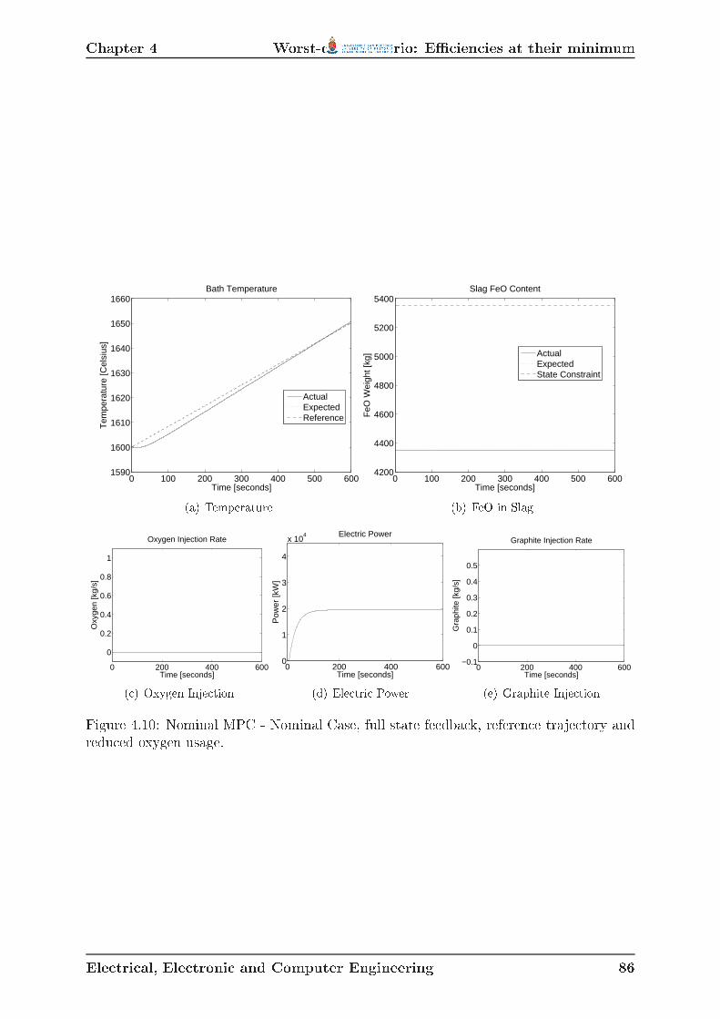
Chapter 4 Worst- ase s enario: E ien ies at their minimum
0 100 200 300 400 500 6001590
1600
1610
1620
1630
1640
1650
1660
Time [seconds]
Tem
pera
ture
[Cel
sius
]
Bath Temperature
ActualExpectedReference
(a) Temperature 0 100 200 300 400 500 6004200
4400
4600
4800
5000
5200
5400
Time [seconds]
FeO
Wei
ght [
kg]
Slag FeO Content
ActualExpectedState Constraint
(b) FeO in Slag0 200 400 600
0
0.2
0.4
0.6
0.8
1
Time [seconds]
Oxy
gen
[kg/
s]
Oxygen Injection Rate
( ) Oxygen Inje tion 0 200 400 6000
1
2
3
4
x 104
Time [seconds]
Pow
er [k
W]
Electric Power
(d) Ele tri Power 0 200 400 600−0.1
0
0.1
0.2
0.3
0.4
0.5
Time [seconds]
Gra
phite
[kg/
s]
Graphite Injection Rate
(e) Graphite Inje tionFigure 4.10: Nominal MPC - Nominal Case, full state feedba k, referen e traje tory andredu ed oxygen usage.
Ele tri al, Ele troni and Computer Engineering 86

Chapter 4 Worst- ase s enario: E ien ies at their minimum
0 100 200 300 400 500 6001600
1610
1620
1630
1640
1650
1660
Time [seconds]
Tem
pera
ture
[Cel
sius
]
Bath Temperature
ActualExpectedReference
(a) Temperature 0 100 200 300 400 500 6004200
4400
4600
4800
5000
5200
5400
Time [seconds]
FeO
Wei
ght [
kg]
Slag FeO Content
ActualExpectedState Constraint
(b) FeO in Slag0 200 400 600
0
0.2
0.4
0.6
0.8
1
Time [seconds]
Oxy
gen
[kg/
s]
Oxygen Injection Rate
( ) Oxygen Inje tion 0 200 400 6000
1
2
3
4
x 104
Time [seconds]
Pow
er [k
W]
Electric Power
(d) Ele tri Power 0 200 400 600−0.1
0
0.1
0.2
0.3
0.4
0.5
Time [seconds]
Gra
phite
[kg/
s]
Graphite Injection Rate
(e) Graphite Inje tionFigure 4.11: Dual Mode Robust MPC - Nominal Case, full state feedba k, referen etraje tory and redu ed oxygen usage.
Ele tri al, Ele troni and Computer Engineering 87

Chapter 4 Worst- ase s enario: E ien ies at their minimumthan nominal e ien ies (ηFeO and ηARC) have on the ontroller and system as a whole.In these s enarios the following assumptions are made:• There are three feedba k s enarios: Full state-feedba k is available. One temperature measurement is available. One temperature measurement and an update of the e ien ies (ηFeO and
ηARC) of the predi tor are available.• The predi tor and a tual plant have a mismat h in their e ien ies (ηFeO and ηARC)where the e ien ies are lower in the real plant than in the predi tor.• There are no disturban es.The three feedba k s enarios help to investigate the performan e of the system withregards to the dierent modules in the system, espe ially the performan e of the predi torand ontroller. One of the obje tives of the ontrollers is to limit the amount of FeO thatforms. Only the s enarios with a higher penalty on oxygen are evaluated here, with theother s enarios evaluated in appendix B.1.1.4.3.1 Worst- ase s enario: E ien ies at their minimum with fullstate feedba kIn this rst instan e, full-state feedba k is employed to evaluate the losed-loop perfor-man e without a predi tor in the loop in the extreme ase where the e ien ies (ηFeOand ηARC) are at the minimum of the model parameter onden e intervals. RobustMPC and nominal MPC are ompared to determine whether robust MPC provides betterperforman e in the presen e of model mismat h ompared to nominal MPC.A setpoint of 1650oC for temperature as well as higher weighting on oxygen inje tion(table 4.2) is used for the rst set of simulations.From these results (gures 4.12 and 4.13) it is lear that the robust MPC performsbetter than the nominal MPC. The robust ontroller produ ed a smaller steady-stateEle tri al, Ele troni and Computer Engineering 88

Chapter 4 Worst- ase s enario: E ien ies at their minimumtemperature oset. It is interesting to note that the nominal ontroller is stable for thissimulation even in this extreme model mismat h situation. The heavier weighting onoxygen inje tion is not enough to limit the FeO produ tion to below the onstraint limit.The se ond set of simulations uses a referen e traje tory for temperature and a higherweighting on the oxygen inje tion (table 4.2).These results (gures 4.14 and 4.15) show the superior performan e of the robust MPC ompared to the nominal MPC, with almost perfe t tra king of the referen e traje toryby the robust MPC. The higher weighting on the oxygen auses the FeO onstraint to berea hed mu h later and it for es the robust ontroller to use more ele tri ity. The robustMPC used more oxygen, but this resulted in better traje tory following when omparedto results obtained with the nominal MPC.This s enario showed that both ontrollers are stable for the respe tive simulationswith extreme model mismat h, but the robust ontroller showed better performan e interms of setpoint and referen e traje tory following than the nominal ontroller.4.3.2 Worst- ase s enario: E ien ies at their minimum with oneplant measurementA more realisti feedba k s enario is investigated, be ause typi ally only one measurementof temperature is taken in the middle of the rening stage. The rest of the data is produ edby the predi tor. The predi tor uses the nominal plant parameters, while the real plantuses the worst- ase s enario where the e ien ies (ηFeO and ηARC) are at their minimum.This s enario should shed light on the ee t of model mismat h between the predi torand real plant when ompared to the results of the previous subse tion.A setpoint of 1650oC for temperature as well as higher weighting on oxygen inje tion(table 4.2) is used for the rst set of simulations.Figures 4.16 and 4.17 show that both ontrollers perform equally poorly as a result ofthe ina urate feedba k from the predi tor. An a eptable margin on the tap temperatureis ±100C, whi h both the ontrollers were unable to attain.A referen e traje tory for temperature as well as higher weighting on oxygen inje tionEle tri al, Ele troni and Computer Engineering 89

Chapter 4 Worst- ase s enario: E ien ies at their minimum
0 100 200 300 400 500 6001600
1610
1620
1630
1640
1650
Time [seconds]
Tem
pera
ture
[Cel
sius
]
Bath Temperature
ActualExpectedReference
(a) Temperature 0 100 200 300 400 500 6004200
4400
4600
4800
5000
5200
5400
Time [seconds]
FeO
Wei
ght [
kg]
Slag FeO Content
ActualExpectedState Constraint
(b) FeO in Slag0 200 400 600
0
0.2
0.4
0.6
0.8
1
Time [seconds]
Oxy
gen
[kg/
s]
Oxygen Injection Rate
( ) Oxygen Inje tion 0 200 400 6000
1
2
3
4
x 104
Time [seconds]
Pow
er [k
W]
Electric Power
(d) Ele tri Power 0 200 400 600−0.1
0
0.1
0.2
0.3
0.4
0.5
Time [seconds]
Gra
phite
[kg/
s]
Graphite Injection Rate
(e) Graphite Inje tionFigure 4.12: Nominal MPC - E ien ies at a minimum, full-state feedba k and redu edoxygen usage.
Ele tri al, Ele troni and Computer Engineering 90

Chapter 4 Worst- ase s enario: E ien ies at their minimum
0 100 200 300 400 500 6001600
1610
1620
1630
1640
1650
Time [seconds]
Tem
pera
ture
[Cel
sius
]
Bath Temperature
ActualExpectedReference(a) Temperature 0 100 200 300 400 500 600
4200
4400
4600
4800
5000
5200
5400
Time [seconds]
FeO
Wei
ght [
kg]
Slag FeO Content
ActualExpectedState Constraint
(b) FeO in Slag0 200 400 600
0
0.2
0.4
0.6
0.8
1
Time [seconds]
Oxy
gen
[kg/
s]
Oxygen Injection Rate
( ) Oxygen Inje tion 0 200 400 6000
1
2
3
4
x 104
Time [seconds]
Pow
er [k
W]
Electric Power
(d) Ele tri Power 0 200 400 600−0.1
0
0.1
0.2
0.3
0.4
0.5
Time [seconds]
Gra
phite
[kg/
s]
Graphite Injection Rate
(e) Graphite Inje tionFigure 4.13: Dual-mode robust MPC - E ien ies at a minimum, full-state feedba k andredu ed oxygen usage.
Ele tri al, Ele troni and Computer Engineering 91

Chapter 4 Worst- ase s enario: E ien ies at their minimum
0 100 200 300 400 500 6001590
1600
1610
1620
1630
1640
1650
Time [seconds]
Tem
pera
ture
[Cel
sius
]
Bath Temperature
ActualExpectedReference
(a) Temperature 0 100 200 300 400 500 6004200
4400
4600
4800
5000
5200
5400
Time [seconds]
FeO
Wei
ght [
kg]
Slag FeO Content
ActualExpectedState Constraint
(b) FeO in Slag0 200 400 600
0
0.2
0.4
0.6
0.8
1
Time [seconds]
Oxy
gen
[kg/
s]
Oxygen Injection Rate
( ) Oxygen Inje tion 0 200 400 6000
1
2
3
4
x 104
Time [seconds]
Pow
er [k
W]
Electric Power
(d) Ele tri Power 0 200 400 600−0.1
0
0.1
0.2
0.3
0.4
0.5
Time [seconds]
Gra
phite
[kg/
s]
Graphite Injection Rate
(e) Graphite Inje tionFigure 4.14: Nominal MPC - E ien ies at a minimum, full-state feedba k, redu edoxygen usage and referen e traje tory.
Ele tri al, Ele troni and Computer Engineering 92

Chapter 4 Worst- ase s enario: E ien ies at their minimum
0 100 200 300 400 500 6001590
1600
1610
1620
1630
1640
1650
1660
Time [seconds]
Tem
pera
ture
[Cel
sius
]
Bath Temperature
ActualExpectedReference
(a) Temperature 0 100 200 300 400 500 6004200
4400
4600
4800
5000
5200
5400
Time [seconds]
FeO
Wei
ght [
kg]
Slag FeO Content
ActualExpectedState Constraint
(b) FeO in Slag0 200 400 600
0
0.2
0.4
0.6
0.8
1
Time [seconds]
Oxy
gen
[kg/
s]
Oxygen Injection Rate
( ) Oxygen Inje tion 0 200 400 6000
1
2
3
4
x 104
Time [seconds]
Pow
er [k
W]
Electric Power
(d) Ele tri Power 0 200 400 600−0.1
0
0.1
0.2
0.3
0.4
0.5
Time [seconds]
Gra
phite
[kg/
s]
Graphite Injection Rate
(e) Graphite Inje tionFigure 4.15: Dual-mode robust MPC - E ien ies at a minimum, full-state feedba k,redu ed oxygen usage and referen e traje tory.
Ele tri al, Ele troni and Computer Engineering 93

Chapter 4 Worst- ase s enario: E ien ies at their minimum
0 100 200 300 400 500 6001600
1610
1620
1630
1640
1650
Time [seconds]
Tem
pera
ture
[Cel
sius
]Bath Temperature
ActualExpectedReference
(a) Temperature 0 100 200 300 400 500 6004200
4400
4600
4800
5000
5200
5400
Time [seconds]
FeO
Wei
ght [
kg]
Slag FeO Content
ActualExpectedState Constraint
(b) FeO in Slag0 200 400 600
0
0.2
0.4
0.6
0.8
1
Time [seconds]
Oxy
gen
[kg/
s]
Oxygen Injection Rate
( ) Oxygen Inje tion 0 200 400 6000
1
2
3
4
x 104
Time [seconds]
Pow
er [k
W]
Electric Power
(d) Ele tri Power 0 200 400 600−0.1
0
0.1
0.2
0.3
0.4
0.5
Time [seconds]
Gra
phite
[kg/
s]
Graphite Injection Rate
(e) Graphite Inje tionFigure 4.16: Nominal MPC - E ien ies at a minimum, one measurement and redu edoxygen usage.(table 4.2) is used for the se ond set of simulations.
These simulations (gures 4.18 and 4.19) show that the robust ontroller manages totra e the referen e better when ompared to the nominal ontroller, but that it is stilloutside the a eptable interval of ±100C. Both ontrollers using a referen e traje tory onaverage steer the temperature ve degrees further from the desired nal value omparedto when a setpoint is employed. The higher weighting on the oxygen auses less FeOto be produ ed by both ontrollers and limits the FeO ontent to within the onstraintlimit.Ele tri al, Ele troni and Computer Engineering 94

Chapter 4 Worst- ase s enario: E ien ies at their minimum
0 100 200 300 400 500 6001600
1610
1620
1630
1640
1650
Time [seconds]
Tem
pera
ture
[Cel
sius
]
Bath Temperature
ActualExpectedReference
(a) Temperature 0 100 200 300 400 500 6004200
4400
4600
4800
5000
5200
5400
Time [seconds]
FeO
Wei
ght [
kg]
Slag FeO Content
ActualExpectedState Constraint(b) FeO in Slag
0 200 400 600
0
0.2
0.4
0.6
0.8
1
Time [seconds]
Oxy
gen
[kg/
s]
Oxygen Injection Rate
( ) Oxygen Inje tion 0 200 400 6000
1
2
3
4
x 104
Time [seconds]
Pow
er [k
W]
Electric Power
(d) Ele tri Power 0 200 400 600−0.1
0
0.1
0.2
0.3
0.4
0.5
Time [seconds]
Gra
phite
[kg/
s]
Graphite Injection Rate
(e) Graphite Inje tionFigure 4.17: Dual-mode robust MPC - E ien ies at a minimum, one measurement andredu ed oxygen usage.
Ele tri al, Ele troni and Computer Engineering 95

Chapter 4 Worst- ase s enario: E ien ies at their minimum
0 100 200 300 400 500 6001590
1600
1610
1620
1630
1640
1650
1660
Time [seconds]
Tem
pera
ture
[Cel
sius
]
Bath Temperature
ActualExpectedReference(a) Temperature 0 100 200 300 400 500 600
4200
4400
4600
4800
5000
5200
5400
Time [seconds]
FeO
Wei
ght [
kg]
Slag FeO Content
ActualExpectedState Constraint
(b) FeO in Slag0 200 400 600
0
0.2
0.4
0.6
0.8
1
Time [seconds]
Oxy
gen
[kg/
s]
Oxygen Injection Rate
( ) Oxygen Inje tion 0 200 400 6000
1
2
3
4
x 104
Time [seconds]
Pow
er [k
W]
Electric Power
(d) Ele tri Power 0 200 400 600−0.1
0
0.1
0.2
0.3
0.4
0.5
Time [seconds]
Gra
phite
[kg/
s]
Graphite Injection Rate
(e) Graphite Inje tionFigure 4.18: Nominal MPC - E ien ies at a minimum, one measurement, referen etraje tory and redu ed oxygen usage.
Ele tri al, Ele troni and Computer Engineering 96

Chapter 4 Worst- ase s enario: E ien ies at their minimum
0 100 200 300 400 500 6001590
1600
1610
1620
1630
1640
1650
1660
Time [seconds]
Tem
pera
ture
[Cel
sius
]
Bath Temperature
ActualExpectedReference(a) Temperature 0 100 200 300 400 500 600
4200
4400
4600
4800
5000
5200
5400
Time [seconds]
FeO
Wei
ght [
kg]
Slag FeO Content
ActualExpectedState Constraint
(b) FeO in Slag0 200 400 600
0
0.2
0.4
0.6
0.8
1
Time [seconds]
Oxy
gen
[kg/
s]
Oxygen Injection Rate
( ) Oxygen Inje tion 0 200 400 6000
1
2
3
4
x 104
Time [seconds]
Pow
er [k
W]
Electric Power
(d) Ele tri Power 0 200 400 600−0.1
0
0.1
0.2
0.3
0.4
0.5
Time [seconds]
Gra
phite
[kg/
s]
Graphite Injection Rate
(e) Graphite Inje tionFigure 4.19: Dual-mode robust MPC - E ien ies at a minimum, one measurement,referen e traje tory and redu ed oxygen usage.
Ele tri al, Ele troni and Computer Engineering 97

Chapter 4 Worst- ase s enario: E ien ies at their minimum4.3.3 Worst- ase s enario: E ien ies at their minimum with oneplant measurement and predi tor parameter updateIn the previous se tion, the ee t of model mismat h between the predi tor and the a tualplant on the performan e of the losed-loop system is made lear. To ombat this, theparameters of the predi tor are updated ea h time a measurement is taken, in an attemptto improve performan e. In this s enario only one temperature measurement is taken inthe middle of the rening stage, with the rest of the state data produ ed by the predi tor.The predi tor uses the nominal plant parameters until the rst measurement is taken,after whi h the orre ted parameters are employed. The real plant uses the worst- ases enario where the e ien ies (ηFeO and ηARC) are at their minimum.A setpoint of 1650oC for temperature as well as higher weighting on oxygen inje tion(table 4.2) is used for the rst set of simulations.Figures 4.20 and 4.21 show that both ontrollers are able to steer the temperature towithin the desired margin of ±100C. The robust ontroller overshoots the setpoint, whi h an be attributed to an over orre tion made in the predi tor, as seen from the expe tedtraje tory ompared to the a tual traje tory. The expe ted traje tory of the robust MPCends at the desired setpoint, while the expe ted traje tory of the nominal MPC endswell outside the a epted margin of ±100C. The nominal MPC steers the temperatureto within the a epted margin of ±100C, but only be ause of an over orre tion of thepredi tor. Both ontrollers use less oxygen, but the nominal ontroller less than therobust ontroller.A referen e traje tory for temperature as well as higher weighting on oxygen inje tion(table 4.2) is used for the fourth set of simulations.These simulations (gures 4.22 and 4.23) show that the nominal ontroller misses the±100C margin, while the robust ontroller does rea h the ±100C margin. The expe tedtraje tory of the robust ontroller rea hes the desired value exa tly, but the a tual valueis somewhat lower, due to an under orre tion in the parameters of the predi tor. The ex-pe ted traje tory of the nominal MPC barely rea hes the a epted margin, but the a tualtraje tory misses the interval ompletely, due to the under orre tion in the parameters ofEle tri al, Ele troni and Computer Engineering 98

Chapter 4 Worst- ase s enario: E ien ies at their minimum
0 100 200 300 400 500 6001600
1610
1620
1630
1640
1650
Time [seconds]
Tem
pera
ture
[Cel
sius
]Bath Temperature
ActualExpectedReference(a) Temperature 0 100 200 300 400 500 600
4200
4400
4600
4800
5000
5200
5400
Time [seconds]
FeO
Wei
ght [
kg]
Slag FeO Content
ActualExpectedState Constraint
(b) FeO in Slag0 200 400 600
0
0.2
0.4
0.6
0.8
1
Time [seconds]
Oxy
gen
[kg/
s]
Oxygen Injection Rate
( ) Oxygen Inje tion 0 200 400 6000
1
2
3
4
x 104
Time [seconds]
Pow
er [k
W]
Electric Power
(d) Ele tri Power 0 200 400 600−0.1
0
0.1
0.2
0.3
0.4
0.5
Time [seconds]
Gra
phite
[kg/
s]
Graphite Injection Rate
(e) Graphite Inje tionFigure 4.20: Nominal MPC - E ien ies at a minimum, one measurement and predi torparameter update and redu ed oxygen usage.the predi tor. The performan e of the nominal MPC is hindered by its onservative useof oxygen.The inability of the ontrollers to follow the referen e is due to an under orre tionof the parameters of the predi tor. The rst sets of results show that the parameters ofthe predi tor are su iently orre ted at the measurement point to enable satisfa toryresults. In the referen e traje tory simulations, the orre tions to the parameters of thepredi tor are insu ient, whi h would require the updater to be tuned dierently for thesetpoint ase and the referen e traje tory ase. The updater is sensitive to the timingof the measurement, the initial onditions that vary for ea h tap, and other disturban essu h as late ave-ins.Ele tri al, Ele troni and Computer Engineering 99

Chapter 4 Worst- ase s enario: E ien ies at their minimum
0 100 200 300 400 500 6001600
1610
1620
1630
1640
1650
1660
Time [seconds]
Tem
pera
ture
[Cel
sius
]
Bath Temperature
ActualExpectedReference
(a) Temperature 0 100 200 300 400 500 6004200
4400
4600
4800
5000
5200
5400
Time [seconds]
FeO
Wei
ght [
kg]
Slag FeO Content
ActualExpectedState Constraint(b) FeO in Slag
0 200 400 600
0
0.2
0.4
0.6
0.8
1
Time [seconds]
Oxy
gen
[kg/
s]
Oxygen Injection Rate
( ) Oxygen Inje tion 0 200 400 6000
1
2
3
4
x 104
Time [seconds]
Pow
er [k
W]
Electric Power
(d) Ele tri Power 0 200 400 600−0.1
0
0.1
0.2
0.3
0.4
0.5
Time [seconds]
Gra
phite
[kg/
s]
Graphite Injection Rate
(e) Graphite Inje tionFigure 4.21: Dual-mode robust MPC - E ien ies at a minimum, one measurement andpredi tor parameter update and redu ed oxygen usage.
Ele tri al, Ele troni and Computer Engineering 100

Chapter 4 Worst- ase s enario: E ien ies at their minimum
0 100 200 300 400 500 6001590
1600
1610
1620
1630
1640
1650
Time [seconds]
Tem
pera
ture
[Cel
sius
]
Bath Temperature
ActualExpectedReference(a) Temperature 0 100 200 300 400 500 600
4200
4400
4600
4800
5000
5200
5400
Time [seconds]
FeO
Wei
ght [
kg]
Slag FeO Content
ActualExpectedState Constraint
(b) FeO in Slag0 200 400 600
0
0.2
0.4
0.6
0.8
1
Time [seconds]
Oxy
gen
[kg/
s]
Oxygen Injection Rate
( ) Oxygen Inje tion 0 200 400 6000
1
2
3
4
x 104
Time [seconds]
Pow
er [k
W]
Electric Power
(d) Ele tri Power 0 200 400 600−0.1
0
0.1
0.2
0.3
0.4
0.5
Time [seconds]
Gra
phite
[kg/
s]
Graphite Injection Rate
(e) Graphite Inje tionFigure 4.22: Nominal MPC - E ien ies at a minimum, one measurement and predi torparameter update, referen e traje tory and redu ed oxygen usage.
Ele tri al, Ele troni and Computer Engineering 101

Chapter 4 Worst- ase s enario: E ien ies at their minimum
0 100 200 300 400 500 6001590
1600
1610
1620
1630
1640
1650
1660
Time [seconds]
Tem
pera
ture
[Cel
sius
]
Bath Temperature
ActualExpectedReference(a) Temperature 0 100 200 300 400 500 600
4200
4400
4600
4800
5000
5200
5400
Time [seconds]
FeO
Wei
ght [
kg]
Slag FeO Content
ActualExpectedState Constraint
(b) FeO in Slag0 200 400 600
0
0.2
0.4
0.6
0.8
1
Time [seconds]
Oxy
gen
[kg/
s]
Oxygen Injection Rate
( ) Oxygen Inje tion 0 200 400 6000
1
2
3
4
x 104
Time [seconds]
Pow
er [k
W]
Electric Power
(d) Ele tri Power 0 200 400 600−0.1
0
0.1
0.2
0.3
0.4
0.5
Time [seconds]
Gra
phite
[kg/
s]
Graphite Injection Rate
(e) Graphite Inje tionFigure 4.23: Dual-mode robust MPC - E ien ies at a minimum, one measurement andpredi tor parameter update, referen e traje tory and redu ed oxygen usage.
Ele tri al, Ele troni and Computer Engineering 102

Chapter 4 Worst- ase s enario: E ien ies at their maximum4.4 Worst- ase s enario: E ien ies at their maximumThese worst- ase s enarios investigate the ee t of model mismat h between the internalmodel of the ontrollers and the a tual plant as well as the predi tor and the a tual plant.This s enario fo uses on the ee t reated if the e ien ies (ηFeO and ηARC) are higherthan nominal. This is a more theoreti al s enario, be ause e ien ies do not tend tobe higher than expe ted, but are ne essary to determine whether the ontroller would beable to ope with su h a situation. In these s enarios the following assumptions are made:• There are three feedba k s enarios: Full state-feedba k is available. One temperature measurement is available. One temperature measurement and an update of predi tor parameters areavailable.• The predi tor and a tual plant have a mismat h in their e ien ies (ηFeO and ηARC)where the e ien ies are higher in the real plant than in the predi tor.• There are no disturban es.The three feedba k s enarios help to investigate the performan e of the system withregards to the dierent modules in the system, espe ially the performan e of the predi torand ontroller.4.4.1 Worst- ase s enario: E ien ies at their maximum withfull state feedba kIn this rst instan e, full-state feedba k is employed to evaluate the losed-loop perfor-man e without a predi tor present, in the extreme ase where the e ien ies (ηFeO and
ηARC) are at the maximum of the onden e interval for the plant model. Robust MPCand nominal MPC are ompared to determine whi h provides better performan e in thepresen e of model mismat h.Ele tri al, Ele troni and Computer Engineering 103
Chapter 4 Worst- ase s enario: E ien ies at their maximumThe rst set of simulations uses a setpoint of 1650oC for temperature as well as higherweighting on oxygen inje tion (table 4.2).Figures 4.24 and 4.25 show that both ontrollers are apable of following the setpoint,and the in reased weighting on oxygen redu es the amount of FeO that forms. Thenominal MPC overshoots the temperature setpoint, while the robust MPC does not. Thenominal MPC uses less oxygen than the robust MPC, whi h result in less FeO formingin the slag.The se ond set of simulations uses a referen e traje tory for temperature as well as ahigher weighting on oxygen inje tion (table 4.2).The last simulations (gures 4.22 and 4.23) show that both ontrollers have goodreferen e following, with the robust ontroller overshooting slightly. The oxygen usage ofthe nominal ontroller is slightly lower than the previous run, but signi antly lower thanthat of the robust ontroller.Both ontrollers perform very well in this s enario where the e ien ies are higherthan expe ted, and do not show any di ulty with the model mismat h between theinternal model and the a tual plant.4.4.2 Worst- ase s enario: E ien ies at their maximum withone plant measurementA more realisti feedba k s enario is investigated, where only one measurement of tem-perature is taken in the middle of the rening stage, the rest of the data is produ ed by apredi tor. The predi tor uses the nominal plant parameters, while the real plant uses theworst- ase s enario where the e ien ies (ηFeO and ηARC) are at their maximum. Thiss enario should shed light on the ee t of model mismat h between the predi tor and realplant when ompared to the results of the previous se tion.The rst set of simulations uses a setpoint of 1650oC for temperature as well as higherweighting on oxygen inje tion (table 4.2).Figures 4.28 and 4.29 show that both ontrollers fail to steer the temperature to withinthe ±100C margin. The ontrollers overshoot the setpoint, be ause the e ien ies (ηFeOEle tri al, Ele troni and Computer Engineering 104

Chapter 4 Worst- ase s enario: E ien ies at their maximum
0 100 200 300 400 500 6001600
1610
1620
1630
1640
1650
1660
Time [seconds]
Tem
pera
ture
[Cel
sius
]
Bath Temperature
ActualExpectedReference
(a) Temperature 0 100 200 300 400 500 6004200
4400
4600
4800
5000
5200
5400
Time [seconds]
FeO
Wei
ght [
kg]
Slag FeO Content
ActualExpectedState Constraint
(b) FeO in Slag0 200 400 600
0
0.2
0.4
0.6
0.8
1
Time [seconds]
Oxy
gen
[kg/
s]
Oxygen Injection Rate
( ) Oxygen Inje tion 0 200 400 6000
1
2
3
4
x 104
Time [seconds]
Pow
er [k
W]
Electric Power
(d) Ele tri Power 0 200 400 600−0.1
0
0.1
0.2
0.3
0.4
0.5
Time [seconds]
Gra
phite
[kg/
s]
Graphite Injection Rate
(e) Graphite Inje tionFigure 4.24: Nominal MPC - E ien ies at maximum with full state feedba k and redu edoxygen usage.
Ele tri al, Ele troni and Computer Engineering 105

Chapter 4 Worst- ase s enario: E ien ies at their maximum
0 100 200 300 400 500 6001600
1610
1620
1630
1640
1650
Time [seconds]
Tem
pera
ture
[Cel
sius
]
Bath Temperature
ActualExpectedReference
(a) Temperature 0 100 200 300 400 500 6004200
4400
4600
4800
5000
5200
5400
Time [seconds]
FeO
Wei
ght [
kg]
Slag FeO Content
ActualExpectedState Constraint
(b) FeO in Slag0 200 400 600
0
0.2
0.4
0.6
0.8
1
Time [seconds]
Oxy
gen
[kg/
s]
Oxygen Injection Rate
( ) Oxygen Inje tion 0 200 400 6000
1
2
3
4
x 104
Time [seconds]
Pow
er [k
W]
Electric Power
(d) Ele tri Power 0 200 400 600−0.1
0
0.1
0.2
0.3
0.4
0.5
Time [seconds]
Gra
phite
[kg/
s]
Graphite Injection Rate
(e) Graphite Inje tionFigure 4.25: Dual-mode robust MPC - E ien ies at maximum with full state feedba kand redu ed oxygen usage.
Ele tri al, Ele troni and Computer Engineering 106

Chapter 4 Worst- ase s enario: E ien ies at their maximum
0 100 200 300 400 500 6001590
1600
1610
1620
1630
1640
1650
1660
Time [seconds]
Tem
pera
ture
[Cel
sius
]
Bath Temperature
ActualExpectedReference
(a) Temperature 0 100 200 300 400 500 6004200
4400
4600
4800
5000
5200
5400
Time [seconds]
FeO
Wei
ght [
kg]
Slag FeO Content
ActualExpectedState Constraint
(b) FeO in Slag0 200 400 600
0
0.2
0.4
0.6
0.8
1
Time [seconds]
Oxy
gen
[kg/
s]
Oxygen Injection Rate
( ) Oxygen Inje tion 0 200 400 6000
1
2
3
4
x 104
Time [seconds]
Pow
er [k
W]
Electric Power
(d) Ele tri Power 0 200 400 600−0.1
0
0.1
0.2
0.3
0.4
0.5
Time [seconds]
Gra
phite
[kg/
s]
Graphite Injection Rate
(e) Graphite Inje tionFigure 4.26: Nominal MPC - E ien ies at maximum with full state feedba k, referen etraje tory and redu ed oxygen usage.
Ele tri al, Ele troni and Computer Engineering 107

Chapter 4 Worst- ase s enario: E ien ies at their maximum
0 100 200 300 400 500 6001600
1610
1620
1630
1640
1650
1660
Time [seconds]
Tem
pera
ture
[Cel
sius
]
Bath Temperature
ActualExpectedReference
(a) Temperature 0 100 200 300 400 500 6004200
4400
4600
4800
5000
5200
5400
Time [seconds]
FeO
Wei
ght [
kg]
Slag FeO Content
ActualExpectedState Constraint
(b) FeO in Slag0 200 400 600
0
0.2
0.4
0.6
0.8
1
Time [seconds]
Oxy
gen
[kg/
s]
Oxygen Injection Rate
( ) Oxygen Inje tion 0 200 400 6000
1
2
3
4
x 104
Time [seconds]
Pow
er [k
W]
Electric Power
(d) Ele tri Power 0 200 400 600−0.1
0
0.1
0.2
0.3
0.4
0.5
Time [seconds]
Gra
phite
[kg/
s]
Graphite Injection Rate
(e) Graphite Inje tionFigure 4.27: Dual-mode robust MPC - E ien ies at maximum with full state feedba k,referen e traje tory and redu ed oxygen usage.
Ele tri al, Ele troni and Computer Engineering 108

Chapter 4 Temperature disturban eand ηARC) are higher than expe ted and the ontrollers drive the temperature too high.The measurement shows the ontrollers that the temperature is too high, and they respondby turning o all energy sour es. The temperature is lowered, but is limited by the tempoof natural heat loss, whi h is too slow to rea h the target by the end of the rening stage.The pro ess ould be a elerated by opening the furna e roof, whi h would aid heat loss.This situation an be prevented by taking a measurement earlier in the rening stage toidentify the problem sooner.The se ond set of simulations uses a referen e traje tory for temperature as well ashigher weighting on oxygen inje tion (table 4.2) and updates the parameters (ηFeO andηARC) of the predi tor from the plant measurement.These simulations (gures 4.30 and 4.31) show that both ontrollers steer the temper-ature to within the ±100C margin. The referen e traje tory auses the temperature toin rease mu h slower than with the setpoint, so that by the time a measurement is taken,the temperature has not yet passed the desired nal value of 16500C. The temperaturedoes in rease above the referen e, and after the measurement, the ontroller orre ts theproblem and on e it has rea hed the referen e, it follows it more losely. There is still anunder orre tion, whi h auses the temperature to in rease faster than expe ted. The nalvalue ends within the a epted ±100C margin. The heavier weighting on oxygen inje tionusage results in lower FeO produ tion without ae ting the temperature response.4.5 Temperature disturban eA temperature disturban e an o ur due to a late ave-in. This happens when thereis solid s rap that falls into the bath, whi h is unexpe ted, be ause it is assumed thatall s rap has melted when rening ommen es. As a result, the bath temperature dropsqui kly, and an be modelled by a step disturban e on the temperature. The followingassumptions are used for this simulation:
• One measurement from the plant.• No predi tor parameters update.Ele tri al, Ele troni and Computer Engineering 109

Chapter 4 Temperature disturban e
0 100 200 300 400 500 6001600
1610
1620
1630
1640
1650
1660
1670
1680
Time [seconds]
Tem
pera
ture
[Cel
sius
]
Bath Temperature
ActualExpectedReference(a) Temperature 0 100 200 300 400 500 600
4200
4400
4600
4800
5000
5200
5400
Time [seconds]
FeO
Wei
ght [
kg]
Slag FeO Content
ActualExpectedState Constraint
(b) FeO in Slag0 200 400 600
0
0.2
0.4
0.6
0.8
1
Time [seconds]
Oxy
gen
[kg/
s]
Oxygen Injection Rate
( ) Oxygen Inje tion 0 200 400 6000
1
2
3
4
x 104
Time [seconds]
Pow
er [k
W]
Electric Power
(d) Ele tri Power 0 200 400 600−0.1
0
0.1
0.2
0.3
0.4
0.5
Time [seconds]
Gra
phite
[kg/
s]
Graphite Injection Rate
(e) Graphite Inje tionFigure 4.28: Nominal MPC - E ien ies at maximum, one measurement and redu edoxygen usage.
Ele tri al, Ele troni and Computer Engineering 110
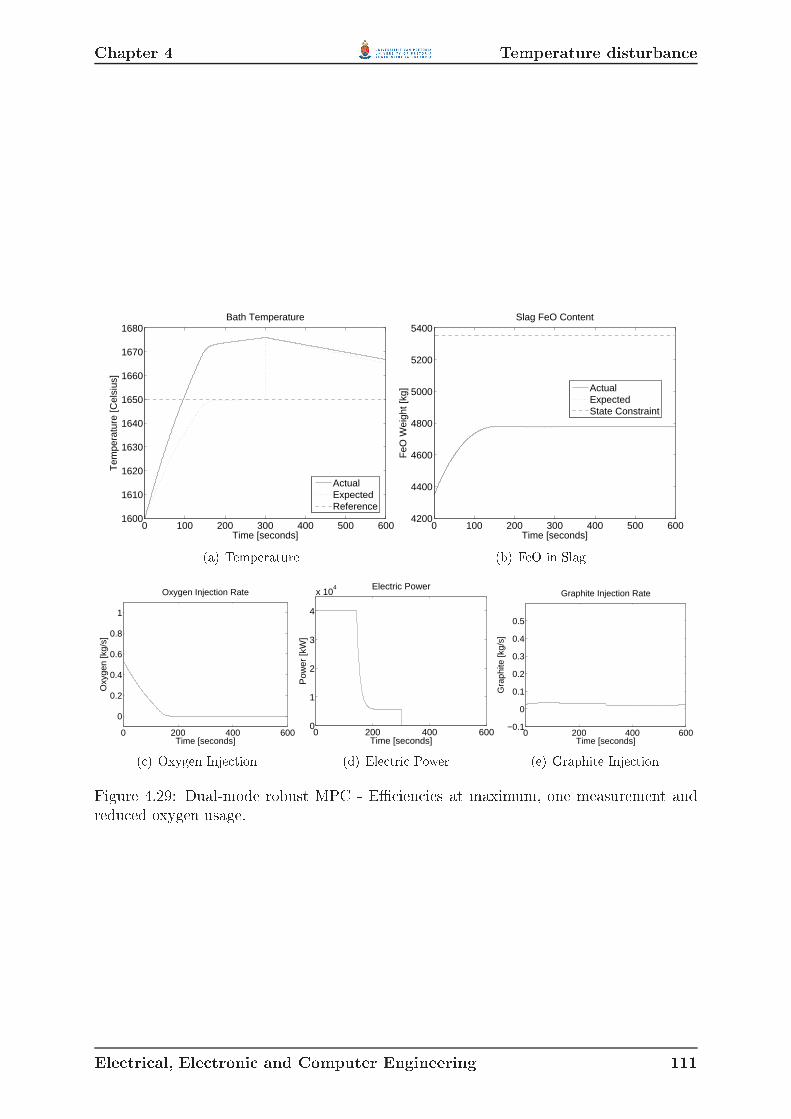
Chapter 4 Temperature disturban e
0 100 200 300 400 500 6001600
1610
1620
1630
1640
1650
1660
1670
1680
Time [seconds]
Tem
pera
ture
[Cel
sius
]
Bath Temperature
ActualExpectedReference(a) Temperature 0 100 200 300 400 500 600
4200
4400
4600
4800
5000
5200
5400
Time [seconds]
FeO
Wei
ght [
kg]
Slag FeO Content
ActualExpectedState Constraint
(b) FeO in Slag0 200 400 600
0
0.2
0.4
0.6
0.8
1
Time [seconds]
Oxy
gen
[kg/
s]
Oxygen Injection Rate
( ) Oxygen Inje tion 0 200 400 6000
1
2
3
4
x 104
Time [seconds]
Pow
er [k
W]
Electric Power
(d) Ele tri Power 0 200 400 600−0.1
0
0.1
0.2
0.3
0.4
0.5
Time [seconds]
Gra
phite
[kg/
s]
Graphite Injection Rate
(e) Graphite Inje tionFigure 4.29: Dual-mode robust MPC - E ien ies at maximum, one measurement andredu ed oxygen usage.
Ele tri al, Ele troni and Computer Engineering 111

Chapter 4 Temperature disturban e
0 100 200 300 400 500 6001590
1600
1610
1620
1630
1640
1650
1660
Time [seconds]
Tem
pera
ture
[Cel
sius
]
Bath Temperature
ActualExpectedReference
(a) Temperature 0 100 200 300 400 500 6004200
4400
4600
4800
5000
5200
5400
Time [seconds]
FeO
Wei
ght [
kg]
Slag FeO Content
ActualExpectedState Constraint
(b) FeO in Slag0 200 400 600
0
0.2
0.4
0.6
0.8
1
Time [seconds]
Oxy
gen
[kg/
s]
Oxygen Injection Rate
( ) Oxygen Inje tion 0 200 400 6000
1
2
3
4
x 104
Time [seconds]
Pow
er [k
W]
Electric Power
(d) Ele tri Power 0 200 400 600−0.1
0
0.1
0.2
0.3
0.4
0.5
Time [seconds]
Gra
phite
[kg/
s]
Graphite Injection Rate
(e) Graphite Inje tionFigure 4.30: Nominal MPC - E ien ies at maximum, one measurement and predi torupdate, referen e traje tory and redu ed oxygen usage.
Ele tri al, Ele troni and Computer Engineering 112

Chapter 4 Temperature disturban e
0 100 200 300 400 500 6001600
1610
1620
1630
1640
1650
1660
Time [seconds]
Tem
pera
ture
[Cel
sius
]
Bath Temperature
ActualExpectedReference
(a) Temperature 0 100 200 300 400 500 6004200
4400
4600
4800
5000
5200
5400
Time [seconds]
FeO
Wei
ght [
kg]
Slag FeO Content
ActualExpectedState Constraint
(b) FeO in Slag0 200 400 600
0
0.2
0.4
0.6
0.8
1
Time [seconds]
Oxy
gen
[kg/
s]
Oxygen Injection Rate
( ) Oxygen Inje tion 0 200 400 6000
1
2
3
4
x 104
Time [seconds]
Pow
er [k
W]
Electric Power
(d) Ele tri Power 0 200 400 600−0.1
0
0.1
0.2
0.3
0.4
0.5
Time [seconds]
Gra
phite
[kg/
s]
Graphite Injection Rate
(e) Graphite Inje tionFigure 4.31: Dual-mode robust MPC - E ien ies at maximum, one measurement andpredi tor update, referen e traje tory and redu ed oxygen usage.
Ele tri al, Ele troni and Computer Engineering 113

Chapter 4 Temperature disturban e
0 100 200 300 400 500 6001600
1610
1620
1630
1640
1650
Time [seconds]
Tem
pera
ture
[Cel
sius
]Bath Temperature
ActualExpectedReference(a) Temperature 0 100 200 300 400 500 600
4200
4400
4600
4800
5000
5200
5400
Time [seconds]
FeO
Wei
ght [
kg]
Slag FeO Content
ActualExpectedState Constraint
(b) FeO in Slag0 200 400 600
0
0.2
0.4
0.6
0.8
1
Time [seconds]
Oxy
gen
[kg/
s]
Oxygen Injection Rate
( ) Oxygen Inje tion 0 200 400 6000
1
2
3
4
x 104
Time [seconds]
Pow
er [k
W]
Electric Power
(d) Ele tri Power 0 200 400 600−0.1
0
0.1
0.2
0.3
0.4
0.5
Time [seconds]
Gra
phite
[kg/
s]
Graphite Injection Rate
(e) Graphite Inje tionFigure 4.32: Dual-mode robust MPC - Temperature disturban e of −200C at time 200swith setpoint of 16500C.• A tual plant and predi tor use nominal plant parameters.• Disturban e of −200C on temperature at time 200s.The rst simulation uses a setpoint of 16500C for temperature and even weighting on theinputs (table 4.2) with a temperature disturban e of −200C at time 200s.Figure 4.32 shows that the robust ontroller is apable of handling a quite severetemperature drop of 200C and re over from it.The se ond simulation uses a referen e traje tory for temperature with even weightingon the inputs (table 4.2) with a temperature disturban e of −200C at time 200s.Figure 4.33 shows that the robust ontroller is apable of handling a quite severetemperature drop of 200C and re over from it even when employing a referen e traje tory.The ontroller makes full use of the energy sour es when the disturban e is dete ted.Ele tri al, Ele troni and Computer Engineering 114

Chapter 4 Temperature disturban e
0 100 200 300 400 500 6001590
1600
1610
1620
1630
1640
1650
1660
Time [seconds]
Tem
pera
ture
[Cel
sius
]
Bath Temperature
ActualExpectedReference
(a) Temperature 0 100 200 300 400 500 6004200
4400
4600
4800
5000
5200
5400
Time [seconds]
FeO
Wei
ght [
kg]
Slag FeO Content
ActualExpectedState Constraint
(b) FeO in Slag0 200 400 600
0
0.2
0.4
0.6
0.8
1
Time [seconds]
Oxy
gen
[kg/
s]
Oxygen Injection Rate
( ) Oxygen Inje tion 0 200 400 6000
1
2
3
4
x 104
Time [seconds]
Pow
er [k
W]
Electric Power
(d) Ele tri Power 0 200 400 600−0.1
0
0.1
0.2
0.3
0.4
0.5
Time [seconds]
Gra
phite
[kg/
s]
Graphite Injection Rate
(e) Graphite Inje tionFigure 4.33: Dual-mode robust MPC - Temperature disturban e of −200C at time 200swith a referen e traje tory for temperature.
Ele tri al, Ele troni and Computer Engineering 115

Chapter 4 SummaryIn the limited feedba k s enarios, the disturban e will only be dete ted when it o ursbefore a measurement, of whi h there is usually only one during the rening stage. Inthis ase, predi tor parameter update will have a detrimental ee t on the performan e,be ause the dieren e would be attributed to model mismat h where the e ien ies arelower than nominal, and an over orre tion would be made to the predi tor. This willresult in the temperature ending up mu h higher than desired.4.6 SummaryThis se tion provides a summary of the results obtained in the previous se tions. Theresults are summarized in tables 4.5, 4.6, 4.7, 4.8 and4.9. The notation used in the tablesis as follows:• Feedba k: FSF - Full state feedba k. OM - One temperature measurement is taken in the middle of the reningstage with the rest of the data produ ed by a predi tor. OMPU - One temperature measurement is taken in the middle of the reningstage with whi h the parameters of the predi tor are updated.• Setpoint or Referen e: Setpoint - A onstant setpoint for temperature of 16500C is employed. Referen e - A linearly in reasing referen e is employed for temperature thatrea hes 16500C at the end of the rening stage period.• Input weighting: Even - All inputs are penalized equally in the obje tive fun tion (table 4.2). Oxygen Heavy (OH) - Oxygen usage is penalized more than the other inputsin the obje tive fun tion (table 4.2).Ele tri al, Ele troni and Computer Engineering 116

Chapter 4 Con lusion• ∆T - Temperature dieren e - The amount that the nal temperature value diersfrom 16500C.• A eptable - If the nal temperature value is within a ±100C margin of 16500C.• Energy usage - The value of a linear penalty fun tion that uses the same weightingsof the inputs as the ontrollers.The energy usage is a fun tion that sums up all the inputs together over the wholeduration of the rening stage. All the inputs are s aled so that the maximum value ofea h ontributes equally to the energy usage metri . This metri gives an indi ation ofhow mu h energy is applied throughout the rening stage for ea h simulation s enario.The metri is al ulated as follows
EU =√
u ∗ R1 ∗ uT (4.1)where R1 is the s aling matrix and u ∈ R600×3 , where there is a sample every se ond over10 minutes and three inputs. The s aling matrix is
R1 =
10 0 0
0 0.00025 0
0 0 20
. (4.2)This gives an indi ation of overall ontroller a tion employed by the ontroller, be ausethe same metri was in luded in the ontroller. The metri an be hanged to in ludeenergy ost that will lead to the most energy e ient solution.4.7 Con lusionThis omprehensive simulation study looked at some theoreti al as well as more pra ti als enarios in order to investigate the performan e of the robust and nominal ontrollers inthe presen e of model mismat h. The performan e of the losed-loop system where thereis model mismat h between the predi tor and a tual plant was also studied.Ele tri al, Ele troni and Computer Engineering 117

Chapter4Con lusion
Table4.5:Summaryofsimulationresultswithnominale ien ies.
Controller Feedba k Setpoint or Referen e Input weighting Temperature dieren e Energy usage FigNominal MPC FSF Setpoint Even < 10C 8.5e+004 4.3Robust MPC FSF Setpoint Even < 10C 1.0e+005 4.4Nominal MPC FSF Setpoint Oxygen Heavy < 10C 1.7e+005 4.6Robust MPC FSF Setpoint Oxygen Heavy < 10C 1.4e+005 4.7Nominal MPC FSF Referen e Even < 10C 8.9e+004 4.8Robust MPC FSF Referen e Even 30C 9.6e+004 4.9Nominal MPC FSF Referen e Oxygen Heavy < 10C 1.8e+005 4.10Robust MPC FSF Referen e Oxygen Heavy 30C 1.7e+005 4.11
Ele tri al,Ele troni andComputerEngineering118

Chapter4Con lusion
Table4.6:Summaryofsimulationresultswithe ien iesattheirminimum.
Controller Feedba k Setpoint or Referen e Input weighting ∆T A eptable Energy usage FigNominal MPC FSF Setpoint Even −20C Yes 2.3e+005 B.1Robust MPC FSF Setpoint Even < 10C Yes 2.3e+005 B.2Nominal MPC FSF Setpoint Oxygen Heavy −20C Yes 3.5e+005 4.12Robust MPC FSF Setpoint Oxygen Heavy < 10C Yes 2.7e+005 4.13Nominal MPC FSF Referen e Even −40C Yes 2.2e+005 B.3Robust MPC FSF Referen e Even < 10C Yes 2.5e+005 B.4Nominal MPC FSF Referen e Oxygen Heavy −50C Yes 3.4e+005 4.14Robust MPC FSF Referen e Oxygen Heavy < 10C Yes 3.5e+005 4.15Nominal MPC OM Setpoint Even −200C No 1.4e+005 B.5Robust MPC OM Setpoint Even −200C No 1.1e+005 B.6Nominal MPC OM Setpoint Oxygen Heavy −230C No 2.4e+005 4.16Robust MPC OM Setpoint Oxygen Heavy −210C No 1.9e+005 4.17Nominal MPC OM Referen e Even −240C No 1.2e+005 B.7Robust MPC OM Referen e Even −220C No 1.3e+005 B.8Nominal MPC OM Referen e Oxygen Heavy −300C No 2.2e+005 4.18Robust MPC OM Referen e Oxygen Heavy −270C No 2.1e+005 4.19Nominal MPC OMPU Setpoint Even −50C Yes 2.2e+005 B.9Robust MPC OMPU Setpoint Even +20C Yes 2.6e+005 B.10Nominal MPC OMPU Setpoint Oxygen Heavy −60C Yes 3.3e+005 4.20Robust MPC OMPU Setpoint Oxygen Heavy +60C Yes 3.0e+005 4.21Nominal MPC OMPU Referen e Even −170C No 1.6e+005 B.11Robust MPC OMPU Referen e Even −120C No 1.9e+005 B.12Nominal MPC OMPU Referen e Oxygen Heavy −190C No 2.7e+005 4.22Robust MPC OMPU Referen e Oxygen Heavy −90C Yes 2.7e+005 4.23
Ele tri al,Ele troni andComputerEngineering119

Chapter4Con lusion
Table4.7:Summaryofsimulationresultswithe ien iesattheirmaximum.
Controller Feedba k Setpoint or Referen e Input weighting ∆T A eptable Energy usage FigNominal MPC FSF Setpoint Even < 10C Yes 4.3e+004 B.13Robust MPC FSF Setpoint Even < 10C Yes 7.4e+004 B.14Nominal MPC FSF Setpoint Oxygen Heavy < 10C Yes 1.1e+005 4.24Robust MPC FSF Setpoint Oxygen Heavy < 10C Yes 9.1e+004 4.25Nominal MPC FSF Referen e Even < 10C Yes 4.3e+004 B.15Robust MPC FSF Referen e Even +40C Yes 5.8e+004 B.16Nominal MPC FSF Referen e Oxygen Heavy < 10C Yes 1.2e+005 4.26Robust MPC FSF Referen e Oxygen Heavy +30C Yes 1.1e+005 4.27Nominal MPC OM Setpoint Even +110C No 6.0e+004 B.17Robust MPC OM Setpoint Even +140C No 8.3e+004 B.18Nominal MPC OM Setpoint Oxygen Heavy +190C No 1.4e+005 4.28Robust MPC OM Setpoint Oxygen Heavy +180C No 1.1e+005 4.29Nominal MPC OM Referen e Even +110C No 5.8e+004 B.19Robust MPC OM Referen e Even +130C No 6.4e+004 B.20Nominal MPC OM Referen e Oxygen Heavy +110C No 1.3e+005 B.21Robust MPC OM Referen e Oxygen Heavy +130C No 1.3e+005 B.22Nominal MPC OMPU Setpoint Even +110C No 6.0e+004 B.23Robust MPC OMPU Setpoint Even +140C No 8.3e+004 B.24Nominal MPC OMPU Setpoint Oxygen Heavy +190C No 1.4e+005 B.25Robust MPC OMPU Setpoint Oxygen Heavy +180C No 1.1e+005 B.26Nominal MPC OMPU Referen e Even +70C Yes 4.9e+004 B.27Robust MPC OMPU Referen e Even +80C Yes 6.0e+004 B.28Nominal MPC OMPU Referen e Oxygen Heavy +50C Yes 1.2e+005 4.30Robust MPC OMPU Referen e Oxygen Heavy +70C Yes 1.2e+005 4.31
Ele tri al,Ele troni andComputerEngineering120

Chapter4Con lusion
Table4.8:Summaryofsimulationresultswithe ien iesatnominalandtemperaturedisturban e.
Controller Feedba k Setpoint or Referen e Input weighting ∆T A eptable Energy usage FigRobust MPC OM Setpoint Even < 10C Yes 1.4e+005 4.32Robust MPC OM Referen e Even +20C Yes 1.4e+005 4.33
Ele tri al,Ele troni andComputerEngineering121

Chapter4Con lusion
Table4.9:Summaryofsimulationresultsthatprodu eda eptableresultsex ludingnominalandfullstatefeedba ks enarios.
Controller Feedba k Setpoint or Referen e Input weighting ∆T E ien ies Energy usage FigNominal MPC OMPU Referen e Even +70C Max 4.9e+004 B.27Robust MPC OMPU Referen e Even +80C Max 6.0e+004 B.28Nominal MPC OMPU Referen e Oxygen Heavy +50C Max 1.2e+005 4.30Robust MPC OMPU Referen e Oxygen Heavy +70C Max 1.2e+005 4.31Nominal MPC OMPU Setpoint Even −50C Min 2.2e+005 B.9Robust MPC OMPU Setpoint Even +20C Min 2.6e+005 B.10Nominal MPC OMPU Setpoint Oxygen Heavy −60C Min 3.3e+005 4.20Robust MPC OMPU Setpoint Oxygen Heavy +60C Min 3.0e+005 4.21Robust MPC OMPU Referen e Oxygen Heavy −90C Min 2.7e+005 4.23Robust MPC OM Setpoint Even < 10C Dist 1.4e+005 4.32Robust MPC OM Referen e Even +20C Dist 1.4e+005 4.33
Ele tri al,Ele troni andComputerEngineering122

Chapter 4 Con lusionIn the s enarios where full state feedba k is available, both the dual-mode robustmodel predi tive ontroller and the nominal model predi tive ontroller perform equallywell. The model un ertainty is su h that the nominal ontroller is apable of handlingit satisfa torily. The feedba k robust MPC annot handle asymmetri onstraints su has those present in the EAF rening pro ess. An ad-ho solution to ompensate forthis limitation is to add a onstant disturban e to the inputs. This was not a su essfulstrategy, be ause the inputs have to be driven to their onstraints, whi h the feedba krobust MPC avoids. This prevents the feedba k robust MPC method from su essfullyfollowing the temperature setpoint or referen e.A bigger problem with automating the pro ess is the la k of feedba k from the plant.A predi tor is used to estimate the plant states in order for the ontroller to generate ontrol a tions for the plant. With the limited number of measurements, the ee t ofmodel mismat h between the predi tor and a tual plant has a mu h bigger impa t onthe performan e of the losed-loop system than the ee ts of model un ertainty. Theee ts of model mismat h an be redu ed by using the plant measurement to updatethe predi tor parameters, but this will meet with varying su ess, be ause there is usu-ally only one measurement available during the rening stage from whi h to update theparameters of the predi tor. If a late ave-in o urs, the predi tor will be in orre tlyupdated, whi h will hinder further performan e. The updating of the parameters of thepredi tor was done using an ad-ho method to determine if it will produ e better resultsthan a predi tor without parameter update. The predi tor utilizing this ad-ho methodshows an improvement over the predi tor without parameter updates. A more in-depthstudy is ne essary to design a proper predi tor for the EAF rening pro ess, one thatutilizes better updating methods and takes all other aspe ts into onsideration through amore systemati design. This was not done here, be ause it falls outside the s ope of thisdissertation.Ele tri al, Ele troni and Computer Engineering 123

Chapter 5Con lusions and re ommendations5.1 Summary of dissertationThe main aim of the dissertation was to synthesise a robust and nominal model predi tive ontroller for the ele tri ar furna e rening pro ess and to evaluate the feasibility ofsu h a ontroller through a simulation study. This work is based on a ve state nonlinearmodel that was derived by Rathaba (2004) for the ele tri ar furna e rening stage fromprevious work by Bekker et al. (1999) and Oosthuizen et al. (2001) who reated a fulltwenty-two state nonlinear model of the ele tri ar furna e pro ess.In Chapter 2 the ve state nonlinear model was linearized for use in the model predi -tive ontrollers. A stru tured un ertainty des ription was used to des ribe all the linearmodels that resulted from the un ertain nonlinear model. The linear models were redu edto simplify the ontrollers by eliminating states that are pra ti ally un ontrollable.In Chapter 3 a brief overview was given of the development of stability theory for robustmodel predi tive ontrollers. Two ontrol methods, feedba k robust model predi tive ontrol and dual-mode robust model predi tive ontrol, were examined in more detailwith regards to synthesis and use.In Chapter 4 an extensive simulation study was done on the rening stage of theele tri ar furna e rening pro ess. Simulations were done where full state feedba k wasassumed in order to evaluate the baseline performan e and stability of the robust andnominal ontrollers. Both the nominal and robust ontrollers were stable during all the124

Chapter 5 Con lusionsimulations and performed well under model mismat h. More pra ti al s enarios werealso investigated where there was only a limited number of measurements and a predi torwas employed to estimate the furna e states. Ea h time a measurement was available,the predi tor was orre ted. In an extension, ea h time a measurement was available, thepredi tor was orre ted and its internal model parameters updated to better approximatethe real plant. The simulations show that the la k of feedba k has a far greater ee t onperforman e than model mismat h.5.2 Con lusionA robust model predi tive ontroller seemed appropriate at the onset of this study inorder to expli itly take the model un ertainty into onsideration as part of the ontrollersynthesis. For omparison, a nominal model predi tive ontroller was used to quantifythe advantage of using a robust ontroller. In the a ademi problem it was lear thatthe robust ontrollers were the only ones to su essfully ontrol the un ertain system.The ele tri ar furna e pro ess does not be ome unstable for all the simulations whennominal model predi tive ontrol is used, even under extreme model mismat h. Thenominal model predi tive ontroller is therefore more than adequate for ontrolling thepro ess.The la k of feedba k is a mu h bigger obsta le in automating the ele tri ar furna erening pro ess. The predi tor needs to be very a urate, but with the un ertainty andla k of measurements, it is very di ult to ensure a ura y. More frequent measurementswould need to be taken and improvements need to be made to the updating of the internalmodel of the predi tor to ensure satisfa tory results.The ele tri ar furna e rening pro ess has states that are manipulated by more thanone input. The inputs and ertain states have onstraints. A simple single-input-single-output ontroller will be di ult to tune in order to ontrol the pro ess and the onstraintswill be handled in an ad-ho fashion. A better strategy is to use a multi-variable ontrolsystem that an expli itly take onstraints into a ount, e.g. model predi tive ontrol.This study has shown that it is not ne essary to use robust model predi tive ontrol,Ele tri al, Ele troni and Computer Engineering 125

Further workbe ause the parameter variation does not pose a problem for nominal model predi tive ontrol.Operators are using the ele tri ar furna e daily without ontrol and are able to rea hthe targets more often than not. This study shows that robust model predi tive ontrolhave di ulty to steer the temperature to the desired setpoint with the limited number ofmeasurements available. All simulation, ex ept for the nominal ases, assumed worst- ases enarios. It is therefore likely that the worst- ase s enarios do not o ur frequently inpra ti e and that the performan e of the losed-loop system might be better in reality.The un ertainties in the model might also be overstated and therefore lead to overly onservative results in the simulations.5.3 Further workThere are ertain areas where further work needs to be done in order to make automati ontrol of the furna e pra ti al:• A better predi tor needs to be developed in order to handle the model un ertaintyand take late ave-ins into a ount, by using a more systemati design method andverifying it on real plant data.• Methods should be devised to in rease measurements during the rening stage. Thisis quite a hallenge due to the harsh environment that the furna e operates in. Apossible solution is to develop soft sensors that estimate bath temperature from theo-gas temperature and oolant temperature.Improvements an be made to the ontrol strategy in the following areas:• Add e onomi obje tives to the ontrol by examining: Energy ost of ele tri ity and hemi al sour es as in Oosthuizen et al. (2004). Optimizing yield. Dierent referen e traje tories for temperature and other variables.Ele tri al, Ele troni and Computer Engineering 126

Further work• Safety and environmental impa t.
Ele tri al, Ele troni and Computer Engineering 127

Further work
Ele tri al, Ele troni and Computer Engineering 128

Referen esBekker, J.G., I.K. Craig and P.C. Pistorius (1999). Modelling and simulation of an ele tri ar furna e pro ess. ISIJ International 39(1), 2332.Bellingan, F. (2005). Private Communi ation. Cape Gate. Vanderbijlpark.Billings, S.A. and H. Ni holson (1977). Modelling a three-phase ele tri ar furna e: om-parative ontrol strategies. Applied Mathemati al Modelling 1, 355361.Billings, S.A., F.M. Boland and H. Ni holson (1979). Ele tri ar furna e modeling and ontrol. Automati a 15, 137148.Bitmead, R. R., M. Gevers and V. Wertz (1990). Adaptive optimal ontrol - The thinkingman's GPC. Prenti e-Hall. Englewood Clis, NJ.Boyd, S., L. El Ghaoui, E. Feron and V. Balakrishnan (1994). Linear Matrix Inequalitiesin System and Control Theory. SAIM. Philadelphia.Cama ho, E.F. and C. Bordons (2003). Model Predi tive Control. Vol. Se ond Edition.Springer-Verlag. London, UK.Cameron, A., N. Saxena and K. Broome (1998). Optimizing EAF operations by dynami pro ess simulation. In: 56th Ele tri Furna e Conferen e Pro eedings. ISS Publishers.Warrendale, Pennsylvania. pp. 689696.Casavolaa, A., D. Famularob and G. Franzéa (2004). Robust onstrained predi tive ontrolof un ertain norm-bounded linear systems. Automati a 40, 18651876.129

REFERENCESChen-Wen, L., H. Shyh-Jier and H. Ching-Lien (2000). Fli ker hara teristi s estimationof an AC ele tri ar furna e. Ele tri Power Systems Resear h 54(2), 121130.Clarke, D.W., C. Mohtadi and P.S. Tus (1987a). Generalized predi tive ontrol: Part I:The basi algorithm. Automati a 23(2), 137148.Clarke, D.W., C. Mohtadi and P.S. Tus (1987b). Generalized predi tive ontrol: Part II:Extensions and interpretations. Automati a 23(2), 149160.Collantes-Bellido, R. and T. Gomez (1997). Identi ation and modeling of a three phasear furna e for voltage disturban e simulation. IEEE Transa tions on Power Delivery12(4), 18121817.Cutler, C.R. and B.L. Ramaker (1980). Dynami matrix ontrol - A omputer ontrolalgorithm. In: Pro eedings of the Joint Automati Control Conferen e. Vol. 1. SanFran is o, CA.Cuzzola, F. A., J. C. Geromel and M. Morari (2002). An improved approa h for on-strained robust model predi tive ontrol. Automati a 38, 11831189.De la Pena, D. Munoz, A. Bemporad and C. Filippi (2004). Robust Expli it MPC Basedon Approximate Multi-parametri Convex Programming. In: 43th IEEE Conferen e onDe ision and Control. Atlantis, Paradise Island, Bahamas. pp. 24912496.De Ni olao, G., L. Magni and R. S attolini (1996). On the robustness of re eding horizon ontrol with terminal onstraints. IEEE Transa tions on Automati Control 41(3), 451453.De Vos, B.J. (1993). Optimization of raw material additions for an oxygen-blowing ar furna e. Master's thesis. University of Pretoria. Pretoria, South Afri a.Deo, B. and Boom, R., Eds. (1993). Fundamentals of Steelmaking Metallurgy. Prenti eHall International.Ding, B., Y. Xi and S. Li (2004). A synthesis approa h of on-line onstrained robust modelpredi tive ontrol. Automati a 40, 163167.Ele tri al, Ele troni and Computer Engineering 130

REFERENCESFruehan, R.F., Ed. (1998). The Making, Shaping and Treating of Steel: Steelmaking andRening. 11 ed.. Asso iation of Iron and Steel Engineers.Fukushima, H. and R. R. Bitmead (2005). Robust onstrained predi tive ontrol using omparison model. Automati a 41, 97106.Galgali, R.K., P. Datta, A.K. Ray, Prasad K.K. and H.S. Ray (2001). Redu tion andfoaming of FeO ontaining slag. Ironmaking and Steelmaking 28, 321327.Ge, M., M. Chiu and Q. Wang (2002). Robust PID ontroller design via LMI approa h.Journal of Pro ess Control 12, 313.Gilbert, E. G. and K. T. Tan (1991). Linear systems with state and ontrol onstraints:The theory and appli ation of maximal output admissible sets. IEEE Transa tions onAutomati Control 36(9), 10081020.Goodwin, G.C., S.F. Graebe and M.E. Salgado (2001). Control system design. Prenti eHall. New Jersey.Gou, H., G. Irons and W.K. Lu (1996). A multiphase uid me hani s approa h togas holdup in bath smelting pro esses. Metallurgi al and Materials Transa tions B27B(2), 195201.Guo, D. and G. Irons (2003). Modeling of Radiation intensity in an EAF. In: Third Inter-national Conferen e on CFD in the Minerals Pro ess Industries. Melbourne, Australia.pp. 651659.Holmes, G. and F. Memoli (2001). Operational improvements a hieved in davsteel, uti-lizing the new te hint kt inje tion system and tdr digital regulation: ase study. In:Ele tri Furna e Conferen e Pro eedings. Iron and Steel So iety. pp. 527537.How, J. (2001). OCW - Feedba k Control 16.31 - Topi 12 - State-spa e model features.Massa husetts Institute of Te hnology. Cambridge, Massa husetts, USA.IISI (2003). World steel in gures 2003. Te hni al report. International Iron and SteelInstitute.Ele tri al, Ele troni and Computer Engineering 131

REFERENCESJiang, R. and R.J. Fruehan (1991). Slag foaming in bath smelting. Metallurgi al Trans-a tions B 22(4), 481489.Khan, M.H., E.J. Evenson and O.I. Negru (2003). Results of the Goodfellow EFSOPTMat Birmingham Steel Corp., Seattle, WA, USA. In: Ele tri Furna e Conferen e Pro- eedings. Iron and Steel So iety. pp. 415428.Kimihisa, I. and R.J. Fruehan (1987). Slag foaming in ele tri furna e steelmaking. In:Ele tri Furna e Pro eedings. Iron and Steel So iety. pp. 345351.Kimihisa, I. and R.J. Fruehan (1989a). Study on the foaming of CaO-SiO2-FeO slags: Part1. Foaming parameters and experimental results. Metallurgi al and Materials Transa -tions B 20B, 509514.Kimihisa, I. and R.J. Fruehan (1989b). Study on the foaming of CaO-SiO2-FeO slags: Part2. Dimensional analysis and foaming in iron and steelmaking pro esses. Metallurgi aland Materials Transa tions B 20B, 515521.King, P.E. and M.D. Nyman (1996). Modeling and ontrol of an ele tri ar furna e usinga feedforward arti ial neural network. Journal of Applied Physi s pp. 18721877.Kleimt, B. and S. Kohle (1997). Power onsumption of ele tri ar furna es with post- ombustion. MPT Metallurgi al Plant and Te hnology International 20(3), 5657.Kleinman, B. L. (1970). An easy way to stabilize a linear onstant system. IEEE Trans-a tions on Automati Control 15(12), 693.Kothare, M. V., V. Balakrishnan and M. Morari (1996). Robust onstrained model pre-di tive ontrol using linear matrix inequalities. Automati a 32, 13611379.Kouvaritakis, B., J. A. Rossiter and J. S huurmans (2000). E ient robust predi tive ontrol. IEEE Transa tions on Automati Control 45(8), 145159.Langson, W., I. Chrysso hoos, S. V. Rakovi and D. Q. Mayne (2004). Robust modelpredi tive ontrol using tubes. Automati a 40, 125133.Ele tri al, Ele troni and Computer Engineering 132

REFERENCESLee, E. B. and L. Markus (1967). Foundations of optimal ontrol theory. Wiley. New York.Lee, J. H. and Z. Yu (1997). Worst- ase formulations of model predi tive ontrol forsystems with bounded parameters. Automati a 33(5), 763781.Lee, Y. I. and B. Kouvaritakis (2000). Robust re eding horizon ontrol for systems withun ertain dynami s and input saturation. Automati a 36(10), 14971504.Lee, Y. I. and B. Kouvaritakis (2002). Superposition in e ient robust onstrained pre-di tive ontrol. Automati a 38, 875878.Ma Rosty, R. (2005). Modelling, Optimization and Control of an Ele tri Ar Furna e.PhD thesis. M Master University. Hamilton, Ontario, Canada.Magni, L. and R. Sepul hre (1997). Stability margins of nonlinear re eding-horizon ontrolvia inverse optimality. Systems & Control Letters 32(4), 241245.Magni, L., H. Nijmeijer and A. van der S haft (2001). A re eding horizon approa h to thenonlinear H∞ problem. Automati a 37(3), 429435.Marique, C., P. Nyssen and P. Salamone (1999). On-line ontrol of the foamy slag inEAF. In: Pro eedings of the 6th European Ele tri Steelmaking Conferen e. Düsseldorf.pp. 154161.Matson, S. and W.F. Ramirez (1999). Optimal Operation of an Ele tri Ar Furna e. In:57th Ele tri Furna e Conferen e Pro eedings. ISS Publishers. Warrendale, Pennsylva-nia. pp. 719728.Mayne, D. Q., J. B. Rawlings, C. V. Rao and P. O. M. S okaert (2000). Constrainedmodel predi tive ontrol: Stability and optimality. Automati a 36, 789814.Mayne, D.Q., M.M. Seron and S.V. Rakovi (2005). Robust model predi tive ontrol of onstrained linear systems with bounded disturban es. Automati a 41, 219224.Meng, M. and G. Irons (2000). Comparison of Ele tri Ar Models with Industrial Data.In: 58th Ele tri Furna e Conferen e and 17th Te hnology Conferen e Pro eedings. ISSPublishers. Warrendale, Pennsylvania.Ele tri al, Ele troni and Computer Engineering 133

REFERENCESMi halska, H. and D.Q. Mayne (1993). Robust re eding horizon ontrol of onstrainednonlinear systems. IEEE Transa tions on Automati Control 38(11), 16231633.Modigell, M., A. Traebert and P. Monheim (2001a). A modeling te hnique for metallur-gi al pro esses and its appli ation. AISE Steel Te hnology 28, 4547.Modigell, M., A. Traebert, P. Monheim, S. Peterson and U. Pi kartz (2001b). A new toolfor pro ess modeling of metallurgi al pro esses. Computers & Chemi al Engineering25, 723727.Morales, R.D., A.N. Conejo and H.H. Rodriguez (2002). Pro ess dynami s of ele tri ar furna e during Dire t Redu ed Iron melting. Metallurgi al and Materials Transa tionsB 33B, 187199.Morales, R.D., H. Rodriguez-Hernández and A.N. Conejo (2001a). A mathemati al sim-ulator for the EAF steelmaking pro ess using Dire t Redu ed Iron. ISIJ International41(5), 426435.Morales, R.D., R. Lule, F. López, J. Cama ho and J.A. Romero (2001b). The slag foamingpra ti e in EAF and its inuen e on the steelmaking shop produ tivity. ISIJ Interna-tional 35(9), 10541062.Nyssen, P., C. Marique, C. Prüm, P. Bintner and L. Sivini (1999). A new metallurgi almodel for the ontrol of EAF operations. In: Pro eedings of the 6th European Ele tri Steelmaking Conferen e. Düsseldorf. pp. 4350.Nyssen, P., R. Colin, S. Knoops and J.L. Junque (2002). On-line EAF ontrol with adynami metallurgi al model. In: Pro eedings of the 7th European Ele tri SteelmakingConferen e. Veni e. pp. 293304.Oosthuizen, D.J., I.K. Craig and P.C. Pistorius (2004). E onomi evaluation and designof an ele tri ar furna e ontroller based on e onomi obje tives. Control EngineeringPra ti e 12, 253265.Ele tri al, Ele troni and Computer Engineering 134

REFERENCESOosthuizen, D.J., J.H. Viljoen, I.K. Craig and P.C. Pistorius (2001). Modeling of theogas exit temperature and slag foam depth of an ele tri ar furna e pro ess. ISIJInternational 41(4), 399401.Panno hia, G. (2004). Robust model predi tive ontrol with guaranteed setpoint tra k-ing. Journal of Pro ess Control 14, 927937.Park, M. and H. Rhee (2001). LMI-based robust model predi tive ontrol for a ontinuousMMA polymerization rea tor. Computers & Chemi al Engineering 25, 15131520.Peterka, V. (1984). Predi tor-based self tuning ontrol. Automati a 20(1), 3950.Pluymers, B., J.A. Rossiter, J. Suykens and B. De Moor (2005a). The e ient ompu-tation of polyhedral invariant sets for linear systems with polytopi un ertainty. In:Pro eedings of the Ameri an Control Conferen e 2005,. Portland, USA. pp. 804809.Pluymers, B., J.A. Rossiter, J.A.K. Suykens and B. De Moor (2005b). A simple algorithmfor robust MPC. In: Pro edings of the 16th IFAC World Congress. Prague, Cze hRepubli .Pujadas, A., J. M Cauley and M. Ia uzzi (2003). EAF energy optimization at Nu or Yam-ato Steel. In: ISSTe h 2003 Conferen e Pro eedings. Iron and Steel So iety. pp. 391402.Qin, S. J. and T. A. Badgwell (2003). A survey of industrial model predi tive ontrolte hnology. Control Engineering Pra ti e 11, 733764.Raisz, D., M. Sakulin, H. Renner and Y. Tehlivets (2000). Re ognition of operationalstates in ele tri ar furna es. In: Pro eedings of the Ninth International Conferen e onHarmoni s and Quality of Power. Vol. 2. IEEE. pp. 475480.Rathaba, P.L. (2004). Model tting for an ele tri ar furna e rening. Master's thesis.University of Pretoria. Pretoria, South Afri a.Rawlings, J. B. and K. R. Muske (1993). Stability of onstrained re eding horizon ontrol.Transa tions on Automati Control 38(10), 15121516.Ele tri al, Ele troni and Computer Engineering 135

REFERENCESRi halet, J., A. Rault, J.L. Testud and J. Papon (1978). Model predi tive heuristi ontrol:Appli ations to industrial pro esses. Automati a 14(5), 413428.Rodríguez, P. and D. Dumur (2005). Generalized predi tive ontrol robusti ation un-der frequen y and time-domain onstraints. IEEE Transa tions on Control SystemsTe hnology 13(4), 577587.Rossiter, J. A., B. Kouvaritakis and M. J. Ri e (1998). A numeri ally robust state-spa eapproa h to stable-predi tive ontrol strategies. Automati a 34(1), 6573.S huurmans, J. and J. A. Rossiter (2000). Robust model predi tive ontrol using tightsets of predi ted states. In: IEE Pro eedings - Control Theory and Appli ations. Vol.147. pp. 1318.S okaert, P. O. M. and D. Q. Mayne (1998). Min-max feedba k model predi tive ontrolfor onstrained linear systems. IEEE Transa tions on Automati Control 43(8), 11361142.S okaert, P. O. M., D. Q. Mayne and J. B. Rawlings (1999). Suboptimal model pre-di tive ontrol (feasibility implies stability). IEEE Transa tions on Automati Control44(3), 648654.Tang, X., M. Kirs hen and H.P. Abel (2003). Modelling of EAF Ogas Post Combustionin Dedusting Systems using CFD Methods. Steel Resear h 74(4), 201210.Taylor, C.R., Ed. (1985). Ele tri Furna e Steelmaking. Iron and Steel So iety.Thomson, M.J., N.G. Kournetas, E. Evenson, I.D. Sommerville, M Lean A. and GuerardJ. (2001). Ee t of Oxyfuel burner ratio hanges on energy e ien y in ele tri ar furna e at Co-Steel Las o. Ironmaking and Steelmaking 28, 267272.Traebert, A., M. Modigell, P. Monheim and K. Ha k (1999). Development of a mod-elling te hnique for non-equilibrium metallurgi al pro esses. S andanavian Journal ofMetallurgy 28, 285290.Ele tri al, Ele troni and Computer Engineering 136

REFERENCESTsai, P., J. Chu, S. Jang and S. Shieh (2002). Developing a robust model predi tive ontrolar hite ture through regional knowledge analysis of arti ial neural networks. Journalof Pro ess Control 13(5), 423435.Turkdogan, E.T. (1989). Fundamentals of Steelmaking. Institute of Materials. London.Wan, Z. and M. V. Kothare (2003). An e ient o-line formulation of robust modelpredi tive ontrol using linear matrix inequalities. Automati a 39, 837846.Wang, D. and J. A. Romagnoli (2003). Robust model predi tive ontrol design using ageneralized obje tive fun tion. Computers & Chemi al Engineering 27(7), 965982.Wang, Y. J. and J. B. Rawlings (2004a). A new robust model predi tive ontrol methodI: Theory and omputation. Journal of Pro ess Control 14, 231247.Wang, Y. J. and J. B. Rawlings (2004b). A new robust model predi tive ontrol methodII: Examples. Journal of Pro ess Control 14(3), 249262.Wu, F. (2001). LMI-based robust model predi tive ontrol and its appli ation to an in-dustrial CSTR problem. Journal of Pro ess Control 11, 649659.
Ele tri al, Ele troni and Computer Engineering 137

Appendix AA ademi ProblemIn this hapter, an a ademi problem is used to ompare the two robust MPC togetherwith nominal MPC, with respe t to robust stability and performan e. The a ademi problem onsists of a system with greatly varying dynami behaviour, whi h provides anex ellent test of the stability and robustness of the dierent ontrollers.A.1 A ademi problem modelThis a ademi problem was taken from Kothare et al. (1996). The problem is a two-mass-spring system (gure A.1). The system was dis retized using Euler's rst orderapproximation for the derivative with a sampling time of 0.1s. The dis retized system is
Mass 1 Mass 2
K
X1 X2
U
Figure A.1: Coupled mass-spring system.138

Appendix A A ademi problem modelgiven by
x1(k + 1)
x2(k + 1)
x3(k + 1)
x4(k + 1)
=
1 0 0.1 0
0 1 0 0.1
−0.1K/m1 0.1K/m1 1 0
0.1K/m2 −0.1K/m2 0 1
x1(k)
x2(k)
x3(k)
x4(k)
+ (A.1)
0
0
0.1/m1
0
u(k) (A.2)y(k) = x2(k) (A.3)where x1 and x2 are the positions of body 1 and body 2 respe tively and x3 and x4 arethe respe tive velo ities of body 1 and body 2. The mass of body 1 is m1 and the mass ofbody 2 is m2, while K is the spring onstant. The input of the system u is the for e thatis applied to the rst body. The performan e spe i ations an be summarized as follows
• Use onstant mass for body 1 and body 2 of 1 kg: m1 = m2 = 1.• Use an un ertain spring onstant that varies between 0.5 and 10: 0.5 ≤ K ≤ 10.• An input onstraint of |u| ≤ 1 should be maintained.• A output unit step should be followed.• Assume full state feedba k is available.To des ribe the ee t of the un ertain spring onstant K, a stru tured un ertainty de-s ription is used. The stru tured un ertainty des ription has the form
Ω =
[
A + BpδCq B + BpδDqu
] (A.4)where Ω is the system spa e, δ is an operator that varies between -1 and 1, BpCq des ribesthe deviation from the nominal for A, and BpDqu des ribes the deviation from nominalEle tri al, Ele troni and Computer Engineering 139

Appendix A Simulation Resultsfor B.The system in (A.1) an be rewritten as a stru tured un ertainty des ription with the onstant values substituted as:δ =
K − Knom
Kdev
(A.5)A =
1 0 0.1 0
0 1 0 0.1
−0.1Knom 0.1Knom 1 0
0.1Knom −0.1Knom 0 1
(A.6)B =
0
0
0.1
0
(A.7)Bp =
0
0
−0.1
0.1
(A.8)Cq =
[
Kdev −Kdev 0 0
] (A.9)Dqu = 0 (A.10)A.2 Simulation ResultsThree ontrollers were used in the simulation study. The ontroller losed-loop systemstru ture is shown in gure A.2. The feedba k robust model predi tive ontroller is shownrst, the dual-mode robust model predi tive ontroller se ond, and the nominal modelpredi tive ontrol as a ben hmark last. Three simulation s enarios were onsidered:1. The nominal ase where δ = 0.2. Extreme deviation from nominal δ =-1.Ele tri al, Ele troni and Computer Engineering 140

Appendix A Simulation Results4 State
Linear
Plant
(Robust)
Model Predictive
Controller
SetpointPosition of mass 2 Force
- Positions of masses
- Velocity of massesFigure A.2: A ademi problem losed-loop system.Table A.1: A ademi problem MPC state and input weighting.Variable Des ription ValueQ State weighting
1 0 0 00 1 0 00 0 1 00 0 0 1
R Input weighting 0.000013. Extreme deviation from nominal δ =1.The nominal s enario gives an indi ation of the onservatism that is introdu ed in orderto robustify the losed loop. The nominal MPC will be the ben hmark with whi h to ompare the two robust ontrollers. The two extreme ases provide a measure of theperforman e of the two robust ontrollers.A.2.1 Nominal s enarioThe nominal s enario uses the nominal model (δ = 0). All the ontrollers use the samestate and input weighting (shown in table A.1) in order to gauge their relative perfor-man e, and to get a feel for the amount of onservatism that is introdu ed in order torobustify the ontrollers.These results (gures A.3 and A.4) show that the nominal MPC gives the best per-forman e when δ = 0. This is to be expe ted, be ause the robust ontrollers are moreEle tri al, Ele troni and Computer Engineering 141

Appendix A Simulation Results
0 20 40 600
0.2
0.4
0.6
0.8
1
Time [seconds]
Sta
te 1
State Response 1
DRMPCFRMPCReference
0 20 40 600
0.2
0.4
0.6
0.8
1
Time [seconds]S
tate
2
State Response 2
DRMPCFRMPCReference
0 20 40 60−0.1
0
0.1
0.2
0.3
Time [seconds]
Sta
te 3
State Response 3
DRMPCFRMPCReference
0 20 40 600
0.05
0.1
0.15
0.2
Time [seconds]
Sta
te 4
State Response 4
DRMPCFRMPCReference
0 20 40 60−1.5
−1
−0.5
0
0.5
1
1.5
Time [seconds]
Inpu
t
Input
DRMPCFRMPC
Figure A.3: Feedba k and Dual-mode Robust MPC - Nominal S enarioEle tri al, Ele troni and Computer Engineering 142

Appendix A Simulation Results
0 20 40 600
0.5
1
1.5
Time [seconds]
Sta
te 1
State Response 1
Nominal MPCReference
0 20 40 600
0.5
1
1.5
Time [seconds]S
tate
2
State Response 2
ActualReference
0 20 40 60−0.1
0
0.1
0.2
0.3
0.4
Time [seconds]
Sta
te 3
State Response 3
Nominal MPCReference
0 20 40 60−0.2
0
0.2
0.4
0.6
Time [seconds]
Sta
te 4
State Response 4
Nominal MPCReference
0 20 40 60−1
−0.5
0
0.5
1
Time [seconds]
Inpu
t
Input
Figure A.4: Nominal MPC - Nominal S enarioEle tri al, Ele troni and Computer Engineering 143

Appendix A Con lusion onservative in order to ensure stability for all the system realizations. The results alsoshow that the feedba k robust model predi tive ontroller gives better performan e thanthe dual-mode robust model predi tive ontroller. The internal, globally stabilizing feed-ba k ontrol employed by the dual-mode ontroller is generated by the feedba k robust ontrol algorithm for the initial state. The feedba k gain was generated without tak-ing the input onstraint into a ount in order to redu e onservatism for the dual-mode ontroller.A.2.2 Extreme deviation δ = −1 and δ = 1The extreme deviation s enarios help gauge the performan e of the robust ontrollers.Both ontrollers use the same weighting on state and input deviation as shown in tableA.1.The results in gure A.5 show that both robust ontrollers are stable in this simulation,be ause the losed-loop system onverges to the setpoints, but the feedba k robust modelpredi tive ontroller delivers better performan e in terms of settling time.The results in gure A.6 mirror the previous on lusion, be ause both robust on-trollers are stable in this simulation, but the feedba k robust model predi tive ontrollerdelivers better performan e in terms of rea hing the desired setpoint as well as overshoot.Figure A.7 shows the performan e of the losed-loop system with nominal MPC. Here itis lear that the losed-loop is unstable for this simulation, be ause the losed-loop systemos illates with in reasing amplitude, and the same result is obtained in the ase whereδ = 1.A.3 Con lusionThe a ademi problem shows the advantage of using robust model predi tive ontrol,where un ertainty auses large variations in dynami behaviour. Both the robust on-trollers were stable for all the simulations over the whole variation in system dynami s,whereas the nominal MPC was unstable in both extreme s enario simulations. The feed-Ele tri al, Ele troni and Computer Engineering 144

Appendix A Con lusion
0 20 40 600
0.2
0.4
0.6
0.8
1
Time [seconds]
Sta
te 1
State Response 1
DRMPCFRMPCReference
0 20 40 600
0.2
0.4
0.6
0.8
1
Time [seconds]S
tate
2
State Response 2
DRMPCFRMPCReference
0 20 40 60−0.1
0
0.1
0.2
0.3
Time [seconds]
Sta
te 3
State Response 3
DRMPCFRMPCReference
0 20 40 600
0.05
0.1
0.15
0.2
Time [seconds]
Sta
te 4
State Response 4
DRMPCFRMPCReference
0 20 40 60−1.5
−1
−0.5
0
0.5
1
1.5
Time [seconds]
Inpu
t
Input
DRMPCFRMPC
Figure A.5: Feedba k and Dual-mode Robust MPC - Extreme s enario δ = 1
Ele tri al, Ele troni and Computer Engineering 145

Appendix A Con lusion
0 20 40 600
0.5
1
1.5
Time [seconds]
Sta
te 1
State Response 1
DRMPCFRMPCReference
0 20 40 600
0.5
1
1.5
Time [seconds]S
tate
2
State Response 2
DRMPCFRMPCReference
0 20 40 60−0.1
0
0.1
0.2
0.3
Time [seconds]
Sta
te 3
State Response 3
DRMPCFRMPCReference
0 20 40 60−0.02
0
0.02
0.04
0.06
0.08
0.1
Time [seconds]
Sta
te 4
State Response 4
DRMPCFRMPCReference
0 20 40 60−1.5
−1
−0.5
0
0.5
1
1.5
Time [seconds]
Inpu
t
Input
DRMPCFRMPC
Figure A.6: Feedba k and Dual-mode Robust MPC - Extreme s enario δ = −1
Ele tri al, Ele troni and Computer Engineering 146
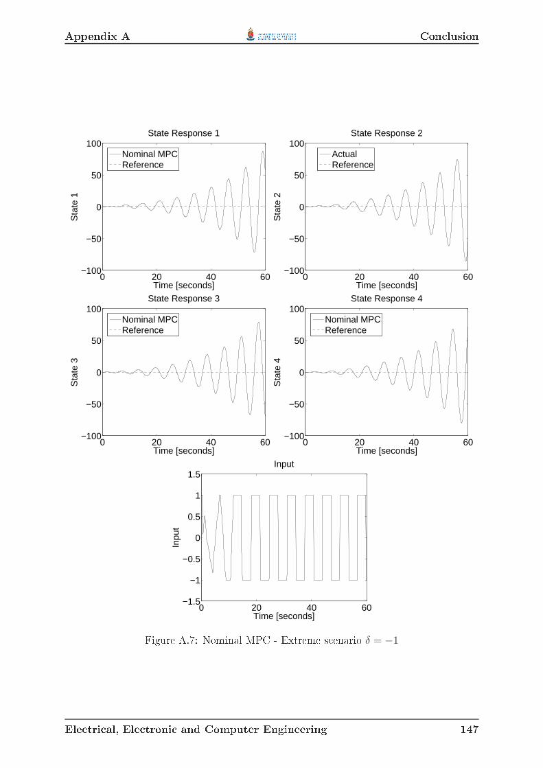
Appendix A Con lusion
0 20 40 60−100
−50
0
50
100
Time [seconds]
Sta
te 1
State Response 1
Nominal MPCReference
0 20 40 60−100
−50
0
50
100
Time [seconds]S
tate
2
State Response 2
ActualReference
0 20 40 60−100
−50
0
50
100
Time [seconds]
Sta
te 3
State Response 3
Nominal MPCReference
0 20 40 60−100
−50
0
50
100
Time [seconds]
Sta
te 4
State Response 4
Nominal MPCReference
0 20 40 60−1.5
−1
−0.5
0
0.5
1
1.5
Time [seconds]
Inpu
t
Input
Figure A.7: Nominal MPC - Extreme s enario δ = −1
Ele tri al, Ele troni and Computer Engineering 147

Appendix A Con lusionba k robust ontroller delivered better performan e than the dual-mode robust ontroller,be ause as the state and inputs approa h 0, the ontroller makes the feedba k gain less onservative. The feedba k ontroller has a problem with non-symmetri input onstraintswhen there is a steady-state other than the origin, be ause the feedba k gain of the on-troller stays onservative and might also lead to large steady-state osets in the states.The behaviour of the dual mode ontroller is greatly inuen ed by the globally stabilizingfeedba k gain K, more so than by the weighting matri es Q and R.
Ele tri al, Ele troni and Computer Engineering 148

Appendix BAuxiliary simulation resultsIn this appendix, all the auxiliary simulation results of hapter 4 are shown with a shortdes ription of the simulation parameters and a short dis ussion of the results. In thisappendix, only the s enarios where there are even weightings on the inputs are evaluated.This gives an indi ation how it will ae t the temperature response if more oxygen isavailable as an energy sour e when ompared to the redu ed oxygen usage s enariosshown in hapter 4.B.1 Worst- ase s enario: E ien ies at their minimumThis s enario fo uses on the ee t that lower than nominal e ien ies (ηFeO and ηARC)have on the ontroller and system as a whole. In this s enario the following assumptionsare made:
• There are three feedba k s enarios: Full state-feedba k is available. One measurement is available. One measurement and update of the e ien ies (ηFeO and ηARC) of the pre-di tor are available.• The predi tor and a tual plant have a mismat h in their e ien ies (ηFeO and ηARC)where the e ien ies are lower in the real plant than in the predi tor.149

Appendix B Worst- ase s enario: E ien ies at their minimum
0 100 200 300 400 500 6001600
1610
1620
1630
1640
1650
Time [seconds]
Tem
pera
ture
[Cel
sius
]Bath Temperature
ActualExpectedReference
(a) Temperature 0 100 200 300 400 500 6004200
4400
4600
4800
5000
5200
5400
Time [seconds]
FeO
Wei
ght [
kg]
Slag FeO Content
ActualExpectedState Constraint
(b) FeO in Slag0 200 400 600
0
0.2
0.4
0.6
0.8
1
Time [seconds]
Oxy
gen
[kg/
s]
Oxygen Injection Rate
( ) Oxygen Inje tion 0 200 400 6000
1
2
3
4
x 104
Time [seconds]
Pow
er [k
W]
Electric Power
(d) Ele tri Power 0 200 400 600−0.1
0
0.1
0.2
0.3
0.4
0.5
Time [seconds]
Gra
phite
[kg/
s]
Graphite Injection Rate
(e) Graphite Inje tionFigure B.1: Nominal MPC - E ien ies at a minimum with full-state feedba k.• There are no disturban es.B.1.1 Worst- ase s enario: Minimum e ien ies with full statefeedba kIn this rst instan e, full-state feedba k is employed to evaluate the losed-loop perfor-man e without a predi tor in the loop, in the extreme ase where the e ien ies (ηFeOand ηARC) are at the minimum of the onden e interval for the plant model. RobustMPC and nominal MPC are ompared to determine whether robust MPC provides betterperforman e in the presen e of model mismat h ompared to nominal MPC.A temperature setpoint of 1650oC as well as even weighting (table 4.2) is used for therst set of simulations.From these result (gures B.1 and B.2), it is lear that the robust MPC performsEle tri al, Ele troni and Computer Engineering 150

Appendix B Worst- ase s enario: E ien ies at their minimum
0 100 200 300 400 500 6001600
1610
1620
1630
1640
1650
Time [seconds]
Tem
pera
ture
[Cel
sius
]
Bath Temperature
ActualExpectedReference(a) Temperature 0 100 200 300 400 500 600
4200
4400
4600
4800
5000
5200
5400
Time [seconds]
FeO
Wei
ght [
kg]
Slag FeO Content
ActualExpectedState Constraint
(b) FeO in Slag0 200 400 600
0
0.2
0.4
0.6
0.8
1
Time [seconds]
Oxy
gen
[kg/
s]
Oxygen Injection Rate
( ) Oxygen Inje tion 0 200 400 6000
1
2
3
4
x 104
Time [seconds]
Pow
er [k
W]
Electric Power
(d) Ele tri Power 0 200 400 600−0.1
0
0.1
0.2
0.3
0.4
0.5
Time [seconds]
Gra
phite
[kg/
s]
Graphite Injection Rate
(e) Graphite Inje tionFigure B.2: Dual-mode robust MPC - E ien ies at a minimum with full-state feedba k.
Ele tri al, Ele troni and Computer Engineering 151

Appendix B Worst- ase s enario: E ien ies at their minimum
0 100 200 300 400 500 6001590
1600
1610
1620
1630
1640
1650
Time [seconds]
Tem
pera
ture
[Cel
sius
]Bath Temperature
ActualExpectedReference
(a) Temperature 0 100 200 300 400 500 6004200
4400
4600
4800
5000
5200
5400
Time [seconds]
FeO
Wei
ght [
kg]
Slag FeO Content
ActualExpectedState Constraint
(b) FeO in Slag0 200 400 600
0
0.2
0.4
0.6
0.8
1
Time [seconds]
Oxy
gen
[kg/
s]
Oxygen Injection Rate
( ) Oxygen Inje tion 0 200 400 6000
1
2
3
4
x 104
Time [seconds]
Pow
er [k
W]
Electric Power
(d) Ele tri Power 0 200 400 600−0.1
0
0.1
0.2
0.3
0.4
0.5
Time [seconds]
Gra
phite
[kg/
s]
Graphite Injection Rate
(e) Graphite Inje tionFigure B.3: Nominal MPC - E ien ies at a minimum, full-state feedba k and referen etraje tory.better than the nominal MPC. The robust ontroller produ ed a smaller steady-stateoset for the temperature. It is interesting to note that the nominal ontroller is stablefor this simulation with extreme model mismat h.A referen e traje tory is used for temperature over the duration of the rening stageas well as even weighting (table 4.2) on the inputs for the se ond set of simulations.These results (gures B.3 and B.4) show that the robust ontroller performs mu hbetter with almost perfe t referen e following ompared to the nominal ontroller. Thenominal ontroller uses mu h less oxygen than the robust ontroller, whi h an a ountfor the di ulty in following the referen e traje tory.Ele tri al, Ele troni and Computer Engineering 152

Appendix B Worst- ase s enario: E ien ies at their minimum
0 100 200 300 400 500 6001590
1600
1610
1620
1630
1640
1650
1660
Time [seconds]
Tem
pera
ture
[Cel
sius
]
Bath Temperature
ActualExpectedReference
(a) Temperature 0 100 200 300 400 500 6004200
4400
4600
4800
5000
5200
5400
Time [seconds]
FeO
Wei
ght [
kg]
Slag FeO Content
ActualExpectedState Constraint
(b) FeO in Slag0 200 400 600
0
0.2
0.4
0.6
0.8
1
Time [seconds]
Oxy
gen
[kg/
s]
Oxygen Injection Rate
( ) Oxygen Inje tion 0 200 400 6000
1
2
3
4
x 104
Time [seconds]
Pow
er [k
W]
Electric Power
(d) Ele tri Power 0 200 400 600−0.1
0
0.1
0.2
0.3
0.4
0.5
Time [seconds]
Gra
phite
[kg/
s]
Graphite Injection Rate
(e) Graphite Inje tionFigure B.4: Dual-mode robust MPC - E ien ies at a minimum, full-state feedba k andreferen e traje tory.
Ele tri al, Ele troni and Computer Engineering 153

Appendix B Worst- ase s enario: E ien ies at their minimum
0 100 200 300 400 500 6001600
1610
1620
1630
1640
1650
Time [seconds]
Tem
pera
ture
[Cel
sius
]Bath Temperature
ActualExpectedReference
(a) Temperature 0 100 200 300 400 500 6004200
4400
4600
4800
5000
5200
5400
Time [seconds]
FeO
Wei
ght [
kg]
Slag FeO Content
ActualExpectedState Constraint
(b) FeO in Slag0 200 400 600
0
0.2
0.4
0.6
0.8
1
Time [seconds]
Oxy
gen
[kg/
s]
Oxygen Injection Rate
( ) Oxygen Inje tion 0 200 400 6000
1
2
3
4
x 104
Time [seconds]
Pow
er [k
W]
Electric Power
(d) Ele tri Power 0 200 400 600−0.1
0
0.1
0.2
0.3
0.4
0.5
Time [seconds]
Gra
phite
[kg/
s]
Graphite Injection Rate
(e) Graphite Inje tionFigure B.5: Nominal MPC - E ien ies at a minimum with one measurement.B.1.2 Worst- ase s enario: Minimum e ien ies with one plantmeasurementIn this s enario only one measurement of temperature is taken in the middle of the reningstage, the rest of the data is produ ed by the predi tor. The predi tor uses the nominalplant parameters, while the real plant uses the worst- ase s enario where the e ien ies(ηFeO and ηARC) are at their minimum. This s enario should shed light on the ee t ofmodel mismat h between the predi tor and real plant model.A setpoint of 1650oC for temperature as well as even weightings on the inputs (table4.2) are used for the rst set of simulations.These results (gures B.5 and B.6) show that both ontrollers perform equally poorly.The ontrollers are under the impression that they have rea hed the desired setpoint as in-di ated by the expe ted line, but in reality the temperature is lower. At the measurementEle tri al, Ele troni and Computer Engineering 154

Appendix B Worst- ase s enario: E ien ies at their minimum
0 100 200 300 400 500 6001600
1610
1620
1630
1640
1650
Time [seconds]
Tem
pera
ture
[Cel
sius
]
Bath Temperature
ActualExpectedReference
(a) Temperature 0 100 200 300 400 500 6004200
4400
4600
4800
5000
5200
5400
Time [seconds]
FeO
Wei
ght [
kg]
Slag FeO Content
ActualExpectedState Constraint
(b) FeO in Slag0 200 400 600
0
0.2
0.4
0.6
0.8
1
Time [seconds]
Oxy
gen
[kg/
s]
Oxygen Injection Rate
( ) Oxygen Inje tion 0 200 400 6000
1
2
3
4
x 104
Time [seconds]
Pow
er [k
W]
Electric Power
(d) Ele tri Power 0 200 400 600−0.1
0
0.1
0.2
0.3
0.4
0.5
Time [seconds]
Gra
phite
[kg/
s]
Graphite Injection Rate
(e) Graphite Inje tionFigure B.6: Dual-mode robust MPC - E ien ies at a minimum with one measurement.
Ele tri al, Ele troni and Computer Engineering 155

Appendix B Worst- ase s enario: E ien ies at their minimum
0 100 200 300 400 500 6001590
1600
1610
1620
1630
1640
1650
1660
Time [seconds]
Tem
pera
ture
[Cel
sius
]Bath Temperature
ActualExpectedReference(a) Temperature 0 100 200 300 400 500 600
4200
4400
4600
4800
5000
5200
5400
Time [seconds]
FeO
Wei
ght [
kg]
Slag FeO Content
ActualExpectedState Constraint
(b) FeO in Slag0 200 400 600
0
0.2
0.4
0.6
0.8
1
Time [seconds]
Oxy
gen
[kg/
s]
Oxygen Injection Rate
( ) Oxygen Inje tion 0 200 400 6000
1
2
3
4
x 104
Time [seconds]
Pow
er [k
W]
Electric Power
(d) Ele tri Power 0 200 400 600−0.1
0
0.1
0.2
0.3
0.4
0.5
Time [seconds]
Gra
phite
[kg/
s]
Graphite Injection Rate
(e) Graphite Inje tionFigure B.7: Nominal MPC - E ien ies at a minimum, one measurement and referen etraje tory.point, the value of the predi tor is orre ted, and the ontrollers respond a ordingly.The nal value is still below the desired value, be ause of the mismat h in the predi tor.An a epted margin of error is 100C ea h way, whi h the ontrollers are not apable ofattaining.A referen e traje tory for temperature as well as even weighting on the inputs (table4.2) is used for the se ond set of simulations.Figures B.7 and B.8 show poor referen e following by both ontrollers due to theina ura y of the predi tor. The expe ted line shows what the ontroller expe ts thevalues to be. The robust ontroller follows the referen e slightly better than the nominal ontroller but still ends below the 100C a epted interval.Ele tri al, Ele troni and Computer Engineering 156

Appendix B Worst- ase s enario: E ien ies at their minimum
0 100 200 300 400 500 6001590
1600
1610
1620
1630
1640
1650
1660
Time [seconds]
Tem
pera
ture
[Cel
sius
]
Bath Temperature
ActualExpectedReference(a) Temperature 0 100 200 300 400 500 600
4200
4400
4600
4800
5000
5200
5400
Time [seconds]
FeO
Wei
ght [
kg]
Slag FeO Content
ActualExpectedState Constraint
(b) FeO in Slag0 200 400 600
0
0.2
0.4
0.6
0.8
1
Time [seconds]
Oxy
gen
[kg/
s]
Oxygen Injection Rate
( ) Oxygen Inje tion 0 200 400 6000
1
2
3
4
x 104
Time [seconds]
Pow
er [k
W]
Electric Power
(d) Ele tri Power 0 200 400 600−0.1
0
0.1
0.2
0.3
0.4
0.5
Time [seconds]
Gra
phite
[kg/
s]
Graphite Injection Rate
(e) Graphite Inje tionFigure B.8: Dual-mode robust MPC - E ien ies at a minimum, one measurement andreferen e traje tory.
Ele tri al, Ele troni and Computer Engineering 157

Appendix B Worst- ase s enario: E ien ies at their maximumB.1.3 Worst- ase s enario: Minimum e ien ies with one plantmeasurement and predi tor parameter updateIn the previous se tion, the ee t of model mismat h between the predi tor and thea tual plant on the performan e of the losed-loop system is lear. To ombat this, theparameters of the predi tor are updated ea h time a measurement is taken, in an attemptto improve performan e. In this s enario only one measurement is taken in the middle ofthe rening stage, the rest of the state data is produ ed by the predi tor. The predi toruses the nominal plant parameters until the rst measurement is taken, after whi h theupdated parameters are employed. The real plant uses the worst- ase s enario where thee ien ies (ηFeO and ηARC) are at their minimum.A setpoint of 1650oC for temperature as well as even weighting on the inputs (table4.2) is used for the rst set of simulations.Figures B.9 and B.10 show that both ontrollers are now able to steer the pro ess towithin the desired ±100C margin. The robust ontroller is able to rea h the desired set-point by the end of the rening stage, whi h is slightly better than the nominal ontroller.A referen e traje tory for temperature as well as even weighting for the inputs (table4.2) is used for the se ond set of simulations.Figures B.11 and B.12 show that neither of the ontrollers an steer the temperature towithin±100C. This is due to an under orre tion made in the predi tor. In both ases, theexpe ted state propagation follows the referen e traje tory, but the a tual performan e ofthe robust ontroller is better than that of the nominal ontroller. The nominal ontrolleruses signi antly less oxygen than the robust ontroller whi h an explain why the robustMPC performs slightly better than the nominal MPC.B.2 Worst- ase s enario: E ien ies at their maximumThis worst- ase s enario investigates the ee t of model mismat h between the internalmodel of the ontrollers and the a tual plant, as well as the predi tor and the a tual plant.This s enario fo uses on the ee t reated if the e ien ies (ηFeO and ηARC) are higherEle tri al, Ele troni and Computer Engineering 158

Appendix B Worst- ase s enario: E ien ies at their maximum
0 100 200 300 400 500 6001600
1610
1620
1630
1640
1650
Time [seconds]
Tem
pera
ture
[Cel
sius
]
Bath Temperature
ActualExpectedReference
(a) Temperature 0 100 200 300 400 500 6004200
4400
4600
4800
5000
5200
5400
Time [seconds]
FeO
Wei
ght [
kg]
Slag FeO Content
ActualExpectedState Constraint
(b) FeO in Slag0 200 400 600
0
0.2
0.4
0.6
0.8
1
Time [seconds]
Oxy
gen
[kg/
s]
Oxygen Injection Rate
( ) Oxygen Inje tion 0 200 400 6000
1
2
3
4
x 104
Time [seconds]
Pow
er [k
W]
Electric Power
(d) Ele tri Power 0 200 400 600−0.1
0
0.1
0.2
0.3
0.4
0.5
Time [seconds]
Gra
phite
[kg/
s]
Graphite Injection Rate
(e) Graphite Inje tionFigure B.9: Nominal MPC - E ien ies at a minimum with one measurement and pre-di tor parameter update.
Ele tri al, Ele troni and Computer Engineering 159

Appendix B Worst- ase s enario: E ien ies at their maximum
0 100 200 300 400 500 6001600
1610
1620
1630
1640
1650
1660
Time [seconds]
Tem
pera
ture
[Cel
sius
]
Bath Temperature
ActualExpectedReference(a) Temperature 0 100 200 300 400 500 600
4200
4400
4600
4800
5000
5200
5400
Time [seconds]
FeO
Wei
ght [
kg]
Slag FeO Content
ActualExpectedState Constraint
(b) FeO in Slag0 200 400 600
0
0.2
0.4
0.6
0.8
1
Time [seconds]
Oxy
gen
[kg/
s]
Oxygen Injection Rate
( ) Oxygen Inje tion 0 200 400 6000
1
2
3
4
x 104
Time [seconds]
Pow
er [k
W]
Electric Power
(d) Ele tri Power 0 200 400 600−0.1
0
0.1
0.2
0.3
0.4
0.5
Time [seconds]
Gra
phite
[kg/
s]
Graphite Injection Rate
(e) Graphite Inje tionFigure B.10: Dual-mode robust MPC - E ien ies at a minimum with one measurementand predi tor parameter update.
Ele tri al, Ele troni and Computer Engineering 160

Appendix B Worst- ase s enario: E ien ies at their maximum
0 100 200 300 400 500 6001590
1600
1610
1620
1630
1640
1650
Time [seconds]
Tem
pera
ture
[Cel
sius
]
Bath Temperature
ActualExpectedReference
(a) Temperature 0 100 200 300 400 500 6004200
4400
4600
4800
5000
5200
5400
Time [seconds]
FeO
Wei
ght [
kg]
Slag FeO Content
ActualExpectedState Constraint
(b) FeO in Slag0 200 400 600
0
0.2
0.4
0.6
0.8
1
Time [seconds]
Oxy
gen
[kg/
s]
Oxygen Injection Rate
( ) Oxygen Inje tion 0 200 400 6000
1
2
3
4
x 104
Time [seconds]
Pow
er [k
W]
Electric Power
(d) Ele tri Power 0 200 400 600−0.1
0
0.1
0.2
0.3
0.4
0.5
Time [seconds]
Gra
phite
[kg/
s]
Graphite Injection Rate
(e) Graphite Inje tionFigure B.11: Nominal MPC - E ien ies at a minimum, one measurement and predi torparameter update and referen e traje tory.
Ele tri al, Ele troni and Computer Engineering 161

Appendix B Worst- ase s enario: E ien ies at their maximum
0 100 200 300 400 500 6001590
1600
1610
1620
1630
1640
1650
1660
Time [seconds]
Tem
pera
ture
[Cel
sius
]
Bath Temperature
ActualExpectedReference
(a) Temperature 0 100 200 300 400 500 6004200
4400
4600
4800
5000
5200
5400
Time [seconds]
FeO
Wei
ght [
kg]
Slag FeO Content
ActualExpectedState Constraint
(b) FeO in Slag0 200 400 600
0
0.2
0.4
0.6
0.8
1
Time [seconds]
Oxy
gen
[kg/
s]
Oxygen Injection Rate
( ) Oxygen Inje tion 0 200 400 6000
1
2
3
4
x 104
Time [seconds]
Pow
er [k
W]
Electric Power
(d) Ele tri Power 0 200 400 600−0.1
0
0.1
0.2
0.3
0.4
0.5
Time [seconds]
Gra
phite
[kg/
s]
Graphite Injection Rate
(e) Graphite Inje tionFigure B.12: Dual-mode robust MPC - E ien ies at a minimum, one measurement andpredi tor parameter update and referen e traje tory.
Ele tri al, Ele troni and Computer Engineering 162

Appendix B Worst- ase s enario: E ien ies at their maximumthan nominal. This is a more theoreti al s enario, be ause e ien ies do not tend to behigher than expe ted, but it is ne essary to determine whether the ontroller would beable to ope with su h a situation. In this s enario the following assumptions are made:• There are three feedba k s enarios: Full state-feedba k is available. One measurement is available. One measurement and update of predi tor parameters are available.• The predi tor and a tual plant have a mismat h in their e ien ies (ηFeO and ηARC)where the e ien ies are higher in the real plant than in the predi tor.• There are no disturban es.B.2.1 Worst- ase s enario: Maximum e ien ies with full statefeedba kIn this rst instan e, full-state feedba k is employed to evaluate the losed-loop perfor-man e without a predi tor present in the extreme ase where the e ien ies (ηFeO and
ηARC) are at the maximum of the onden e interval for the plant model. Robust MPCand nominal MPC are ompared to determine whi h provides better performan e in thepresen e of model mismat h.The rst set of simulations uses a setpoint of 1650oC for temperature as well as evenweighting on the inputs (table 4.2).Figures B.13 and B.14 show that both ontrollers are able to follow the setpoint, andbe ause of the in reased e ien y of the oxygen and ele tri power, less energy is needed,whi h results in both ontrollers keeping the FeO ontent below the onstraint level.The se ond set of simulations uses a referen e traje tory for temperature as well aseven weighting on the inputs (table 4.2).Figures B.15 and B.16 show that both ontrollers have good referen e following. Thenominal ontroller uses mu h less oxygen than the robust ontroller, whi h is evident inEle tri al, Ele troni and Computer Engineering 163

Appendix B Worst- ase s enario: E ien ies at their maximum
0 100 200 300 400 500 6001600
1610
1620
1630
1640
1650
Time [seconds]
Tem
pera
ture
[Cel
sius
]
Bath Temperature
ActualExpectedReference
(a) Temperature 0 100 200 300 400 500 6004200
4400
4600
4800
5000
5200
5400
Time [seconds]
FeO
Wei
ght [
kg]
Slag FeO Content
ActualExpectedState Constraint
(b) FeO in Slag0 200 400 600
0
0.2
0.4
0.6
0.8
1
Time [seconds]
Oxy
gen
[kg/
s]
Oxygen Injection Rate
( ) Oxygen Inje tion 0 200 400 6000
1
2
3
4
x 104
Time [seconds]
Pow
er [k
W]
Electric Power
(d) Ele tri Power 0 200 400 600−0.1
0
0.1
0.2
0.3
0.4
0.5
Time [seconds]
Gra
phite
[kg/
s]
Graphite Injection Rate
(e) Graphite Inje tionFigure B.13: Nominal MPC - E ien ies at maximum with full state feedba k.
Ele tri al, Ele troni and Computer Engineering 164

Appendix B Worst- ase s enario: E ien ies at their maximum
0 100 200 300 400 500 6001600
1610
1620
1630
1640
1650
Time [seconds]
Tem
pera
ture
[Cel
sius
]
Bath Temperature
ActualExpectedReference
(a) Temperature 0 100 200 300 400 500 6004200
4400
4600
4800
5000
5200
5400
Time [seconds]
FeO
Wei
ght [
kg]
Slag FeO Content
ActualExpectedState Constraint
(b) FeO in Slag0 200 400 600
0
0.2
0.4
0.6
0.8
1
Time [seconds]
Oxy
gen
[kg/
s]
Oxygen Injection Rate
( ) Oxygen Inje tion 0 200 400 6000
1
2
3
4
x 104
Time [seconds]
Pow
er [k
W]
Electric Power
(d) Ele tri Power 0 200 400 600−0.1
0
0.1
0.2
0.3
0.4
0.5
Time [seconds]
Gra
phite
[kg/
s]
Graphite Injection Rate
(e) Graphite Inje tionFigure B.14: Dual-mode robust MPC - E ien ies at maximum with full state feedba k.
Ele tri al, Ele troni and Computer Engineering 165

Appendix B Worst- ase s enario: E ien ies at their maximum
0 100 200 300 400 500 6001590
1600
1610
1620
1630
1640
1650
1660
Time [seconds]
Tem
pera
ture
[Cel
sius
]
Bath Temperature
ActualExpectedReference
(a) Temperature 0 100 200 300 400 500 6004200
4400
4600
4800
5000
5200
5400
Time [seconds]
FeO
Wei
ght [
kg]
Slag FeO Content
ActualExpectedState Constraint
(b) FeO in Slag0 200 400 600
0
0.2
0.4
0.6
0.8
1
Time [seconds]
Oxy
gen
[kg/
s]
Oxygen Injection Rate
( ) Oxygen Inje tion 0 200 400 6000
1
2
3
4
x 104
Time [seconds]
Pow
er [k
W]
Electric Power
(d) Ele tri Power 0 200 400 600−0.1
0
0.1
0.2
0.3
0.4
0.5
Time [seconds]
Gra
phite
[kg/
s]
Graphite Injection Rate
(e) Graphite Inje tionFigure B.15: Nominal MPC - E ien ies at maximum with full state feedba k and refer-en e traje tory.
Ele tri al, Ele troni and Computer Engineering 166

Appendix B Worst- ase s enario: E ien ies at their maximum
0 100 200 300 400 500 6001600
1610
1620
1630
1640
1650
1660
Time [seconds]
Tem
pera
ture
[Cel
sius
]
Bath Temperature
ActualExpectedReference
(a) Temperature 0 100 200 300 400 500 6004200
4400
4600
4800
5000
5200
5400
Time [seconds]
FeO
Wei
ght [
kg]
Slag FeO Content
ActualExpectedState Constraint(b) FeO in Slag
0 200 400 600
0
0.2
0.4
0.6
0.8
1
Time [seconds]
Oxy
gen
[kg/
s]
Oxygen Injection Rate
( ) Oxygen Inje tion 0 200 400 6000
1
2
3
4
x 104
Time [seconds]
Pow
er [k
W]
Electric Power
(d) Ele tri Power 0 200 400 600−0.1
0
0.1
0.2
0.3
0.4
0.5
Time [seconds]
Gra
phite
[kg/
s]
Graphite Injection Rate
(e) Graphite Inje tionFigure B.16: Dual-mode robust MPC - E ien ies at maximum with full state feedba kand referen e traje tory.
Ele tri al, Ele troni and Computer Engineering 167

Appendix B Worst- ase s enario: E ien ies at their maximumthe nal values of the FeO ontent. The robust ontroller slightly overshoots the nalvalue for the temperature but is still well within the desired ±100C interval.B.2.2 Worst- ase s enario: E ien ies at their maximum withone plant measurementA more realisti feedba k s enario is investigated, where only one temperature measure-ment is taken in the middle of the rening stage, the rest of the state data is produ edby a predi tor. The predi tor uses the nominal plant parameters, while the real plantuses the worst- ase s enario where the e ien ies (ηFeO and ηARC) are at their maximum.This s enario should shed light on the ee t of model mismat h between the predi torand real plant when ompared to the results of the previous se tion.The rst set of simulations uses a setpoint of 1650oC for temperature as well as evenweighting on the inputs (table 4.2).Figures B.17 and B.18 show that both ontrollers fail to steer the temperature towithin the ±100C margin. The ontrollers overshoot the setpoint, be ause the e ien ies(ηFeO and ηARC) are higher than expe ted and the ontrollers drive the temperature toohigh. The measurement shows the ontrollers that the temperature is too high, and theyrespond by turning o all energy sour es. The temperature is lowered, but is limited bythe tempo of natural heat loss, whi h is too slow to rea h the target by the end of therening stage. The pro ess ould be a elerated by opening the furna e roof, whi h wouldaid heat loss. This situation an be prevented by taking a measurement earlier in therening stage to identify the problem sooner.The se ond set of simulations uses a referen e traje tory for temperature as well aseven weighting on the inputs (table 4.2).Figures B.19 and B.20 show that both ontrollers overshoot the nal temperature withmore than the a epted margin of ±100C. By the time that the measurement is taken,the temperature is still below the desired value, but already higher than the referen e.The ontrollers orre t the problem by steering the temperature ba k to the referen e,but as soon as the error is orre ted, the temperature is again steered faster than theEle tri al, Ele troni and Computer Engineering 168

Appendix B Worst- ase s enario: E ien ies at their maximum
0 100 200 300 400 500 6001600
1610
1620
1630
1640
1650
1660
1670
1680
Time [seconds]
Tem
pera
ture
[Cel
sius
]
Bath Temperature
ActualExpectedReference(a) Temperature 0 100 200 300 400 500 600
4200
4400
4600
4800
5000
5200
5400
Time [seconds]
FeO
Wei
ght [
kg]
Slag FeO Content
ActualExpectedState Constraint
(b) FeO in Slag0 200 400 600
0
0.2
0.4
0.6
0.8
1
Time [seconds]
Oxy
gen
[kg/
s]
Oxygen Injection Rate
( ) Oxygen Inje tion 0 200 400 6000
1
2
3
4
x 104
Time [seconds]
Pow
er [k
W]
Electric Power
(d) Ele tri Power 0 200 400 600−0.1
0
0.1
0.2
0.3
0.4
0.5
Time [seconds]
Gra
phite
[kg/
s]
Graphite Injection Rate
(e) Graphite Inje tionFigure B.17: Nominal MPC - E ien ies at maximum with one measurement.
Ele tri al, Ele troni and Computer Engineering 169

Appendix B Worst- ase s enario: E ien ies at their maximum
0 100 200 300 400 500 6001600
1610
1620
1630
1640
1650
1660
1670
1680
Time [seconds]
Tem
pera
ture
[Cel
sius
]
Bath Temperature
ActualExpectedReference(a) Temperature 0 100 200 300 400 500 600
4200
4400
4600
4800
5000
5200
5400
Time [seconds]
FeO
Wei
ght [
kg]
Slag FeO Content
ActualExpectedState Constraint
(b) FeO in Slag0 200 400 600
0
0.2
0.4
0.6
0.8
1
Time [seconds]
Oxy
gen
[kg/
s]
Oxygen Injection Rate
( ) Oxygen Inje tion 0 200 400 6000
1
2
3
4
x 104
Time [seconds]
Pow
er [k
W]
Electric Power
(d) Ele tri Power 0 200 400 600−0.1
0
0.1
0.2
0.3
0.4
0.5
Time [seconds]
Gra
phite
[kg/
s]
Graphite Injection Rate
(e) Graphite Inje tionFigure B.18: Dual-mode robust MPC - E ien ies at maximum with one measurement.
Ele tri al, Ele troni and Computer Engineering 170

Appendix B Worst- ase s enario: E ien ies at their maximum
0 100 200 300 400 500 6001590
1600
1610
1620
1630
1640
1650
1660
1670
Time [seconds]
Tem
pera
ture
[Cel
sius
]
Bath Temperature
ActualExpectedReference
(a) Temperature 0 100 200 300 400 500 6004200
4400
4600
4800
5000
5200
5400
Time [seconds]
FeO
Wei
ght [
kg]
Slag FeO Content
ActualExpectedState Constraint
(b) FeO in Slag0 200 400 600
0
0.2
0.4
0.6
0.8
1
Time [seconds]
Oxy
gen
[kg/
s]
Oxygen Injection Rate
( ) Oxygen Inje tion 0 200 400 6000
1
2
3
4
x 104
Time [seconds]
Pow
er [k
W]
Electric Power
(d) Ele tri Power 0 200 400 600−0.1
0
0.1
0.2
0.3
0.4
0.5
Time [seconds]
Gra
phite
[kg/
s]
Graphite Injection Rate
(e) Graphite Inje tionFigure B.19: Nominal MPC - E ien ies at maximum, one measurement and referen etraje tory.
Ele tri al, Ele troni and Computer Engineering 171

Appendix B Worst- ase s enario: E ien ies at their maximum
0 100 200 300 400 500 6001600
1610
1620
1630
1640
1650
1660
1670
Time [seconds]
Tem
pera
ture
[Cel
sius
]
Bath Temperature
ActualExpectedReference(a) Temperature 0 100 200 300 400 500 600
4200
4400
4600
4800
5000
5200
5400
Time [seconds]
FeO
Wei
ght [
kg]
Slag FeO Content
ActualExpectedState Constraint
(b) FeO in Slag0 200 400 600
0
0.2
0.4
0.6
0.8
1
Time [seconds]
Oxy
gen
[kg/
s]
Oxygen Injection Rate
( ) Oxygen Inje tion 0 200 400 6000
1
2
3
4
x 104
Time [seconds]
Pow
er [k
W]
Electric Power
(d) Ele tri Power 0 200 400 600−0.1
0
0.1
0.2
0.3
0.4
0.5
Time [seconds]
Gra
phite
[kg/
s]
Graphite Injection Rate
(e) Graphite Inje tionFigure B.20: Dual-mode robust MPC - E ien ies at maximum, one measurement andreferen e traje tory.
Ele tri al, Ele troni and Computer Engineering 172

Appendix B Worst- ase s enario: E ien ies at their maximum
0 100 200 300 400 500 6001590
1600
1610
1620
1630
1640
1650
1660
1670
Time [seconds]
Tem
pera
ture
[Cel
sius
]Bath Temperature
ActualExpectedReference
(a) Temperature 0 100 200 300 400 500 6004200
4400
4600
4800
5000
5200
5400
Time [seconds]
FeO
Wei
ght [
kg]
Slag FeO Content
ActualExpectedState Constraint
(b) FeO in Slag0 200 400 600
0
0.2
0.4
0.6
0.8
1
Time [seconds]
Oxy
gen
[kg/
s]
Oxygen Injection Rate
( ) Oxygen Inje tion 0 200 400 6000
1
2
3
4
x 104
Time [seconds]
Pow
er [k
W]
Electric Power
(d) Ele tri Power 0 200 400 600−0.1
0
0.1
0.2
0.3
0.4
0.5
Time [seconds]
Gra
phite
[kg/
s]
Graphite Injection Rate
(e) Graphite Inje tionFigure B.21: Nominal MPC - E ien ies at maximum, one measurement, referen e tra-je tory and redu ed oxygen usage.referen e.The third set of simulations uses a referen e traje tory for temperature as well ashigher weighting on oxygen inje tion (table 4.2).These simulations (gures B.21 and B.22) show mu h the same trend as the previousset, with the ex eption that both ontrollers use less oxygen, whi h in turn produ es lessFeO, but the robust ontroller uses signi antly less oxygen ompared with the previoussimulation in gure B.20.The model mismat h between the predi tor and the a tual plant in this s enario, ausesthe temperature to overshoot the desired value of 16500C. The ee t an be redu ed bytaking a sample earlier in the rening stage, whi h will minimize the overshoot and givemore time for the bath to ool o. The se ond solution is to use the referen e traje tory,but from the last two simulations it is lear that the predi tor parameters should beEle tri al, Ele troni and Computer Engineering 173

Appendix B Worst- ase s enario: E ien ies at their maximum
0 100 200 300 400 500 6001600
1610
1620
1630
1640
1650
1660
1670
Time [seconds]
Tem
pera
ture
[Cel
sius
]
Bath Temperature
ActualExpectedReference(a) Temperature 0 100 200 300 400 500 600
4200
4400
4600
4800
5000
5200
5400
Time [seconds]
FeO
Wei
ght [
kg]
Slag FeO Content
ActualExpectedState Constraint
(b) FeO in Slag0 200 400 600
0
0.2
0.4
0.6
0.8
1
Time [seconds]
Oxy
gen
[kg/
s]
Oxygen Injection Rate
( ) Oxygen Inje tion 0 200 400 6000
1
2
3
4
x 104
Time [seconds]
Pow
er [k
W]
Electric Power
(d) Ele tri Power 0 200 400 600−0.1
0
0.1
0.2
0.3
0.4
0.5
Time [seconds]
Gra
phite
[kg/
s]
Graphite Injection Rate
(e) Graphite Inje tionFigure B.22: Dual-mode robust MPC - E ien ies at maximum, one measurement, ref-eren e traje tory and redu ed oxygen usage.
Ele tri al, Ele troni and Computer Engineering 174

Appendix B Worst- ase s enario: E ien ies at their maximumupdated to prevent overshoot from o urring after the measurement.B.2.3 Worst- ase s enario: E ien ies at their maximum withone plant measurement and predi tor parameters updateIn the previous se tion, the ee t that model mismat h has on the performan e of thesystem is apparent. To ombat the ee t, the parameters of the predi tor are updatedea h time a measurement is taken, in an attempt to improve performan e. In this s enarioonly one measurement of temperature is taken in the middle of the rening stage, the restof the data is produ ed by the predi tor. The predi tor uses the nominal plant parametersfor the e ien ies (ηFeO and ηARC) until a measurement is taken, after whi h the orre tedparameters are employed. The real plant uses the worst- ase where the e ien ies (ηFeOand ηARC) are at their maximum.The rst set of simulations uses a setpoint of 1650oC for temperature as well as evenweighting on the inputs (table 4.2).Figures B.23 and B.24 show mu h the same results as in se tion 4.4.2. The update inthe predi tor does not aid in a elerating the ooling of the bath. The only solution herewould be to take a measurement earlier in the pro ess.The se ond set of simulations uses a setpoint of 1650oC for temperature as well ashigher weighting on oxygen inje tion (table 4.2).Figures B.25 and B.26 show mu h the same result as the previous simulation wherethe predi tor update does not solve the ooling limitation. The only dieren e is that,where energy is applied, less oxygen is used be ause of the heavier weighting on the oxygeninje tion rate.A referen e traje tory for temperature as well as even weighting on the inputs (table4.2) is used for the third set of simulations.Figures B.27 and B.28 show en ouraging results. The referen e traje tory ausesthe temperature to in rease mu h slower than with the setpoint, so that by the timea measurement is taken, the temperature has not yet passed the desired nal value of16500C. The temperature does in rease above the referen e, and after the measurement,Ele tri al, Ele troni and Computer Engineering 175

Appendix B Worst- ase s enario: E ien ies at their maximum
0 100 200 300 400 500 6001600
1610
1620
1630
1640
1650
1660
1670
1680
Time [seconds]
Tem
pera
ture
[Cel
sius
]
Bath Temperature
ActualExpectedReference(a) Temperature 0 100 200 300 400 500 600
4200
4400
4600
4800
5000
5200
5400
Time [seconds]
FeO
Wei
ght [
kg]
Slag FeO Content
ActualExpectedState Constraint
(b) FeO in Slag0 200 400 600
0
0.2
0.4
0.6
0.8
1
Time [seconds]
Oxy
gen
[kg/
s]
Oxygen Injection Rate
( ) Oxygen Inje tion 0 200 400 6000
1
2
3
4
x 104
Time [seconds]
Pow
er [k
W]
Electric Power
(d) Ele tri Power 0 200 400 600−0.1
0
0.1
0.2
0.3
0.4
0.5
Time [seconds]
Gra
phite
[kg/
s]
Graphite Injection Rate
(e) Graphite Inje tionFigure B.23: Nominal MPC - E ien ies at maximum with one measurement and pre-di tor update.
Ele tri al, Ele troni and Computer Engineering 176

Appendix B Worst- ase s enario: E ien ies at their maximum
0 100 200 300 400 500 6001600
1610
1620
1630
1640
1650
1660
1670
1680
Time [seconds]
Tem
pera
ture
[Cel
sius
]
Bath Temperature
ActualExpectedReference(a) Temperature 0 100 200 300 400 500 600
4200
4400
4600
4800
5000
5200
5400
Time [seconds]
FeO
Wei
ght [
kg]
Slag FeO Content
ActualExpectedState Constraint
(b) FeO in Slag0 200 400 600
0
0.2
0.4
0.6
0.8
1
Time [seconds]
Oxy
gen
[kg/
s]
Oxygen Injection Rate
( ) Oxygen Inje tion 0 200 400 6000
1
2
3
4
x 104
Time [seconds]
Pow
er [k
W]
Electric Power
(d) Ele tri Power 0 200 400 600−0.1
0
0.1
0.2
0.3
0.4
0.5
Time [seconds]
Gra
phite
[kg/
s]
Graphite Injection Rate
(e) Graphite Inje tionFigure B.24: Dual-mode robust MPC - E ien ies at maximum with one measurementand predi tor update.
Ele tri al, Ele troni and Computer Engineering 177

Appendix B Worst- ase s enario: E ien ies at their maximum
0 100 200 300 400 500 6001600
1610
1620
1630
1640
1650
1660
1670
1680
Time [seconds]
Tem
pera
ture
[Cel
sius
]
Bath Temperature
ActualExpectedReference(a) Temperature 0 100 200 300 400 500 600
4200
4400
4600
4800
5000
5200
5400
Time [seconds]
FeO
Wei
ght [
kg]
Slag FeO Content
ActualExpectedState Constraint
(b) FeO in Slag0 200 400 600
0
0.2
0.4
0.6
0.8
1
Time [seconds]
Oxy
gen
[kg/
s]
Oxygen Injection Rate
( ) Oxygen Inje tion 0 200 400 6000
1
2
3
4
x 104
Time [seconds]
Pow
er [k
W]
Electric Power
(d) Ele tri Power 0 200 400 600−0.1
0
0.1
0.2
0.3
0.4
0.5
Time [seconds]
Gra
phite
[kg/
s]
Graphite Injection Rate
(e) Graphite Inje tionFigure B.25: Nominal MPC - E ien ies at maximum, one measurement and predi torupdate and redu ed oxygen usage.
Ele tri al, Ele troni and Computer Engineering 178

Appendix B Worst- ase s enario: E ien ies at their maximum
0 100 200 300 400 500 6001600
1610
1620
1630
1640
1650
1660
1670
1680
Time [seconds]
Tem
pera
ture
[Cel
sius
]
Bath Temperature
ActualExpectedReference(a) Temperature 0 100 200 300 400 500 600
4200
4400
4600
4800
5000
5200
5400
Time [seconds]
FeO
Wei
ght [
kg]
Slag FeO Content
ActualExpectedState Constraint
(b) FeO in Slag0 200 400 600
0
0.2
0.4
0.6
0.8
1
Time [seconds]
Oxy
gen
[kg/
s]
Oxygen Injection Rate
( ) Oxygen Inje tion 0 200 400 6000
1
2
3
4
x 104
Time [seconds]
Pow
er [k
W]
Electric Power
(d) Ele tri Power 0 200 400 600−0.1
0
0.1
0.2
0.3
0.4
0.5
Time [seconds]
Gra
phite
[kg/
s]
Graphite Injection Rate
(e) Graphite Inje tionFigure B.26: Dual-mode robust MPC - E ien ies at maximum, one measurement andpredi tor update and redu ed oxygen usage.
Ele tri al, Ele troni and Computer Engineering 179

Appendix B Worst- ase s enario: E ien ies at their maximum
0 100 200 300 400 500 6001590
1600
1610
1620
1630
1640
1650
1660
Time [seconds]
Tem
pera
ture
[Cel
sius
]
Bath Temperature
ActualExpectedReference
(a) Temperature 0 100 200 300 400 500 6004200
4400
4600
4800
5000
5200
5400
Time [seconds]
FeO
Wei
ght [
kg]
Slag FeO Content
ActualExpectedState Constraint
(b) FeO in Slag0 200 400 600
0
0.2
0.4
0.6
0.8
1
Time [seconds]
Oxy
gen
[kg/
s]
Oxygen Injection Rate
( ) Oxygen Inje tion 0 200 400 6000
1
2
3
4
x 104
Time [seconds]
Pow
er [k
W]
Electric Power
(d) Ele tri Power 0 200 400 600−0.1
0
0.1
0.2
0.3
0.4
0.5
Time [seconds]
Gra
phite
[kg/
s]
Graphite Injection Rate
(e) Graphite Inje tionFigure B.27: Nominal MPC - E ien ies at maximum, one measurement and predi torupdate and referen e traje tory.
Ele tri al, Ele troni and Computer Engineering 180

Appendix B Worst- ase s enario: E ien ies at their maximum
0 100 200 300 400 500 6001600
1610
1620
1630
1640
1650
1660
Time [seconds]
Tem
pera
ture
[Cel
sius
]
Bath Temperature
ActualExpectedReference
(a) Temperature 0 100 200 300 400 500 6004200
4400
4600
4800
5000
5200
5400
Time [seconds]
FeO
Wei
ght [
kg]
Slag FeO Content
ActualExpectedState Constraint
(b) FeO in Slag0 200 400 600
0
0.2
0.4
0.6
0.8
1
Time [seconds]
Oxy
gen
[kg/
s]
Oxygen Injection Rate
( ) Oxygen Inje tion 0 200 400 6000
1
2
3
4
x 104
Time [seconds]
Pow
er [k
W]
Electric Power
(d) Ele tri Power 0 200 400 600−0.1
0
0.1
0.2
0.3
0.4
0.5
Time [seconds]
Gra
phite
[kg/
s]
Graphite Injection Rate
(e) Graphite Inje tionFigure B.28: Dual-mode robust MPC - E ien ies at maximum, one measurement andpredi tor update and referen e traje tory.
Ele tri al, Ele troni and Computer Engineering 181

Appendix B Worst- ase s enario: E ien ies at their maximumthe ontroller orre ts the problem and on e it has rea hed the referen e, it follows itmore losely. There is still an under orre tion, that auses the temperature to in reasefaster than expe ted. The nal value ends within the a epted ±100C margin. Thenominal ontroller uses less oxygen than the robust ontroller as evident from the nalFeO values.
Ele tri al, Ele troni and Computer Engineering 182

Appendix CMeasured bath and slag dataTables C.1 and C.2 show measured bath and slag data for 18 taps. This data were olle ted by Rathaba (2004).
183

AppendixCTableC.1:Measuredbathandslagdata(Rathaba,2004)part1.
Tap # Time % C % Si O2 [ppm Time Temp0C Time % FeO % SiO2 % CaO % MgO % Al2O31 7.05 0.199 0.03 - 7.15 1619 7.04 17.70 18.2 50.53 3.53 5.107.15 0.125 - 219 7.16 1630 7.16 31.55 10.5 43.45 3.33 3.077.16 0.119 - 229 7.20 1678 7.20 36.53 9.08 37.57 3.47 2.737.20 0.043 - 6582 8.14 0.082 0.01 - 8.14 1598 8.11 27.04 13.7 43.74 5.08 3.698.16 0.060 - 448 8.16 1618 8.16 30.25 12.5 43.09 5.42 3.518.18 0.054 - 504 8.18 1638 8.18 39.20 10.3 34.41 5.43 3.018.21 0.039 - 704 8.21 16403 9.10 0.111 0.03 - 9.13 1597 9.10 31.50 13.4 40.13 5.04 4.139.14 0.053 - 514 9.15 1636 9.14 26.21 12.6 46.07 6.38 3.909.17 0.043 - 623 9.18 1631 9.17 31.82 11.4 40.48 6.14 3.484 10.14 0.078 0.02 - 10.14 1594 10.13 32.13 11.6 41.14 5.46 4.3210.20 0.043 - 648 10.20 1610 10.18 29.80 10.7 43.12 5.77 4.1310.21 1658 10.20 31.65 10.1 41.13 5.77 3.785 11.36 0.060 0.02 - 11.37 1586 11.33 37.80 9.85 36.39 5.14 3.4811.42 0.056 - 466 11.42 1602 11.43 38.25 7.58 36.15 5.11 2.7211.44 0.040 - 699 11.44 1658 11.45 38.12 8.10 39.83 5.69 2.916 12.51 0.060 0.03 - 12.53 1615 12.50 43.95 10.8 29.38 5.25 4.1412.55 0.048 0.03 - 12.55 1647 12.53 43.65 10.1 30.32 5.43 3.8412.55 0.026 - 1048 12.56 45.29 9.61 30.21 5.38 3.687 13.43 0.088 0.03 - 13.43 1571 13.40 34.52 11.7 37.95 5.41 5.0013.45 0.071 0.03 - 13.47 1546 13.44 34.81 11.6 37.65 5.49 5.0313.47 0.065 - 376 13.49 1601 13.48 36.35 9.41 32.00 5.71 3.9613.49 0.054 - 481 13.51 161513.55 0.046 - 5728 15.05 0.056 0.03 - 15.07 1630 15.04 37.33 8.96 38.27 8.07 3.8115.07 0.051 0.03 - 15.08 1643 15.06 35.64 9.24 37.74 7.81 3.9215.08 0.037 - 738 15.08 35.06 8.57 34.60 7.30 3.629 16.02 0.157 0.03 - 16.05 1540 15.56 26.96 11.7 40.20 7.23 4.5816.06 0.106 0.03 - 16.08 1615 16.06 26.57 10.6 43.41 7.05 4.2216.08 0.062 - 481 16.10 1636 16.09 27.05 10.2 39.16 6.34 4.0016.09 0.072 0.03 - 16.13 166016.10 0.093 - 29316.13 0.033 - 845
Ele tri al,Ele troni andComputerEngineering184

AppendixCTableC.2:Measuredbathandslagdata(Rathaba,2004)part2.
Tap # Time % C % Si O2 [ppm Time Temp0C Time % FeO % SiO2 % CaO % MgO % Al2O310 17.03 0.078 0.03 - 17.05 1579 17.02 24.57 14.8 42.47 5.31 4.3617.05 0.085 0.03 - 17.07 1614 17.05 23.91 15.0 44.46 5.98 4.5717.09 0.044 - 624 17.09 1647 17.09 25.08 15.2 43.29 6.50 4.6417.09 0.059 0.03 -11 10.37 0.112 0.02 - 10.36 1570 10.43 35.69 11.1 36.17 5.59 3.8310.39 0.034 - 760 10.39 160010.42 0.030 - 894 10.42 163810.44 0.045 - 604 10.44 163112 11.34 0.057 0.02 - 11.41 1566 11.47 36.34 11.6 34.72 6.96 3.8911.45 0.034 - 804 11.45 163111.47 0.031 - 920 11.47 167313 12.43 0.081 0.02 - 12.45 1585 12.50 34.91 10.2 37.55 5.68 3.5912.48 0.042 - 642 12.48 162312.50 0.039 - 678 12.50 162114 13.42 0.115 0.04 - 13.47 1594 14.10 36.18 10.8 34.39 5.48 3.7813.50 0.050 - 531 13.50 161014.08 0.033 - 823 14.05 165814.10 0.030 - 930 14.08 162114.10 165215 14.56 0.068 0.03 - 15.02 1589 15.09 41.95 10.2 34.43 6.04 3.5715.06 0.036 - 861 15.05 162615.09 0.035 - 757 15.06 164115.11 0.030 - 907 15.08 162615.10 165016 16.03 0.075 0.03 - 16.04 1624 16.05 37.33 10.2 37.51 5.83 3.4716.06 0.034 - 861 16.06 164517 16.54 0.080 0.03 - 17.00 1564 17.10 31.93 12.4 39.96 4.31 4.5317.06 0.036 - 356 17.04 156617.08 0.035 - 592 17.06 158817.08 163918 17.56 0.169 0.03 - 18.05 1582 17.10 31.93 11.2 39.96 6.76 4.2018.01 0.093 0.02 - 18.08 161818.09 0.060 - 592 18.09 1661
Ele tri al,Ele troni andComputerEngineering185