Robust Sliding-mode Control of Wind Energy

Conversion Systems for Optimal Power Extraction

via Nonlinear Perturbation Observers

Bo Yang∗, Tao Yu†, Hongchun Shu∗, Jun Dong∗, Lin Jiang‡

Abstract

This paper designs a novel robust sliding-mode control using nonlinear perturbation observers for

wind energy conversion systems (WECS), in which a doubly-fed induction generator (DFIG) is em-

ployed to achieve an optimal power extraction with an improved fault ride-through (FRT) capability.

The strong nonlinearities originated from the aerodynamics of the wind turbine, together with the

generator parameter uncertainties and wind speed randomness, are aggregated into a perturbation

that is estimated online by a sliding-mode state and perturbation observer (SMSPO). Then, the

perturbation estimate is fully compensated by a robust sliding-mode controller so as to provide a

considerable robustness against various modelling uncertainties and to achieve a consistent control

performance under stochastic wind speed variations. Moreover, the proposed approach has an inte-

grated structure thus only the measurement of rotor speed and reactive power is required, while the

classical auxiliary dq-axis current regulation loops can be completely eliminated. Four case studies are

carried out which verify that a more optimal wind power extraction and an enhanced FRT capability

can be realized in comparison with that of conventional vector control (VC), feedback linearization

control (FLC), and sliding-mode control (SMC).

Keyword DFIG, optimal power extraction, FRT, nonlinear perturbation observer, robust sliding-

mode control

∗Bo Yang, Hongchun Shu, and Jun Dong are with the Faculty of Electric Power Engineering, Kunming University ofScience and Technology, 650500, Kunming, China.

†Tao Yu is with with the School of Electric Power Engineering, South China University of Technology, Guangzhou,China. (corresponding author, Email: taoyu1@scut.edu.cn)

‡Lin Jiang is with the Department of Electrical Engineering & Electronics, University of Liverpool, Liverpool, L69 3GJ,United Kingdom.

1

1 Introduction1

Due to the astonishingly ever-increasing population issue and environmental crisis, both the social and2

industrial demands of renewable energy keep growing rapidly in the past decade around the globe. As3

one of the most abundant and mature renewable energy, wind energy conversion systems (WECS) have4

been paid considerable attention and their proportion in nationwide energy production will rise even5

faster in future [1]. Nowadays, the most commonly used wind turbine in WECS is based on doubly-fed6

induction generator (DFIG) because of its noticeable merits: variable speed generation, the reduction of7

mechanical stresses and acoustic noise, as well as the improvement of the power quality [2].8

So far, an enormous variety of studies have been undertaken for DFIG modelling and control, in which9

vector control (VC) incorporated with proportional-integral (PI) loops is the most popular and widely10

recognized framework in industry, thanks to its promising features of decoupling control of active/reactive11

power, simple structure, as well as high reliability [3]. The primary goal of DFIG control system design is12

to optimally extract the wind power under random wind speed variation, which is usually called maximum13

power point tracking (MPPT) [4]. Meanwhile, a fault-ride through (FRT) capability is often required14

so that DFIG can withstand some typical disturbances in power grids [5]. However, one significant15

drawback of VC is that it cannot maintain a consistent control performance when operation conditions16

vary as its PI parameters are determined by the one-point linearization, while DFIG is a highly nonlinear17

system resulted from the fact that it frequently operates under a time-varying and wide operation region18

by stochastic turbulent wind. Several optimal parameter tuning techniques have been examined to19

improve the overall control performance of PI control, such as the differential evolutionary algorithm20

(DE) employed for the performance enhancement of DFIG in the presence of external disturbances [6].21

Reference [7] proposed a meta-heuristic algorithm called grouped grey wolf optimizer to achieve MPPT22

together with an improved FRT capability. In addition, literature [8] adopted particle swarm optimizer23

(PSO) to enhance the building energy performance. Moreover, a genetic algorithm was developed to24

minimize the energy consumption of the hybrid energy storage system in electric vehicle [9].25

On the other hand, plenty of promising alternatives have been investigated attempting to remedy such26

inherent flaws of VC. For example, fuzzy-logic was used to deal with onshore wind farm site selection27

[10]. In reference [11], a feedback linearization control (FLC) was designed for MPPT of DFIG with28

a thorough modal analysis of generator dynamics, which internal dynamics stability is also proved in29

the context of Lyapunov criterion. Besides, both the rotor position and speed are calculated based on30

model reference adaptive system (MRAS) control strategy by [12], such that a fast dynamic response31

without the requirement of flux estimation can be realized. Furthermore, a robust continuous-time32

2

model predictive direct power control of DFIG was proposed via Taylor series expansion for stator current33

prediction, which is directly used to compute the required rotor voltage in order to minimize the difference34

between the actual stator currents and their references over the prediction period [13]. Meanwhile,35

literature [14] developed an internal model state-feedback approach to control the DFIG currents, which is36

able to provide robustness to external disturbances automatically and to eliminate the need of disturbance37

compensation. Additionally, a Lyapunov control theory based controller was devised for rotor speed38

adjustment without any information about wind data or an available anemometer [15]. A nonlinear39

robust power controller based on a hybrid of adaptive pole placement and backstepping was presented40

in [16], which implementation feasibility is validated through field-programmable gate array (FPGA).41

Moreover, an approximate dynamic programming based optimal and adaptive reactive power control42

scheme was applied to remarkably improve the transient stability of power systems with wind farms [17].43

Among all sorts of advanced approaches, sliding-mode control (SMC) is a powerful high-frequency44

switching control scheme for nonlinear systems with various uncertainties and disturbances, which elegant-45

ly features effective disturbance rejection, fast response, and strong robustness [18], thus it is appropriate46

to tackle the above obstacles. In work [19], the dynamics of a small-capacity wind turbine system con-47

nected to the power grid was altered under severe faults of power grids, in which the transient behaviour48

and the performance limit for FRT are discussed by using two protection circuits of an AC-crowbar and49

a DC-Chopper. A high-order SMC was applied which owns prominent advantages of great robustness50

against power grid faults, together with no extra mechanical stress on the wind turbine drive train [20].51

In addition, reference [21] wisely chose a sliding surface that allows the wind turbine to operate very52

closely to the optimal regions, while PSO was used to determine the optimal slope of the sliding surface53

and the switching component amplitude. Further, an intelligent proportional-integral SMC was proposed54

for direct power control of variable-speed constant-frequency wind turbine systems and MPPT under55

several disturbances [22]. Moreover, literature [23] designed a robust fractional-order SMC for MPPT56

and robustness enhancement of DFIG, in which unknown nonlinear disturbances and parameter uncer-57

tainties are estimated via a fractional-order uncertainty estimator while a continuous control strategy is58

developed to realize a chattering-free manner.59

Nevertheless, an essential shortcoming of SMC is its over-conservativeness stemmed from the use of60

upper bound of uncertainties, while these worst conditions in which the perturbation takes its upper61

bound does not usually occur. As a consequence, numerous disturbance/perturbation observer based62

controllers have been examined which aim to provide a more appropriate control performance by real-time63

compensation of the combinatorial effect of various uncertainties and disturbances, e.g., a high-gain state64

3

and perturbation observer (HGSPO) was adopted to estimate the unmodelled dynamics and parameter65

uncertainties of multi-machine power systems equipped with flexible alternating current transmission66

system devices, such that a coordinated adaptive passive control can be realized [24]. Alternatively, a67

nonlinear observer based adaptive disturbance rejection control (ADRC) was proposed to improve the68

power tracking of DFIG under abrupt changes in wind speed, which can be applied for any type of69

optimal active power tracking algorithms [25]. Moreover, reference [26] described a linear ADRC based70

load frequency control (LFC) to maintain generation-load balance and to realize disturbance rejection71

of power systems integrated with DFIG. In work [27], sliding-mode based perturbation observer was72

used to design a nonlinear adaptive controller for power system stability enhancement. On the other73

hand, disturbance observer based SMC was studied for continuous-time linear systems with mismatched74

disturbances or uncertainties [28], while the applications of disturbance/perturbation observer based SMC75

can be referred to the current regulation of voltage source converter based high voltage direct current76

system [29], LFC of power systems with high wind energy penetration [30], position and velocity profile77

tracking control for next-generation servo track writing [31], etc. In addition, a derivative-free nonlinear78

Kalman filter was redesigned as a disturbance observer to estimate additive input disturbances to DFIG,79

which are finally compensated by a feedback controller that enables the generator’s state variables to80

track desirable setpoints [32].81

This paper proposes a perturbation observer based sliding-mode control (POSMC) of DFIG for opti-82

mal power extraction, which novelty and contribution can be summarized as the following four points:83

• The combinatorial effect of wind turbine nonlinearities, generator parameter uncertainties, and wind84

speed randomness is simultaneously estimated online by a sliding-mode state and perturbation observer85

(SMSPO), which is then fully compensated by a robust sliding-mode controller. Thus no accurate system86

model is needed. In contrast, other nonlinear approaches need an accurate system model [11] or can mere-87

ly handle some specific uncertainties, e.g., wind speed uncertainties [15] or parameter uncertainties [16];88

• Only the measurement of rotor speed and reactive power is required by POSMC, while various gener-89

ator variables and parameters are required by references [12, 14]. Hence POSMC is relatively easy to be90

implemented in practice;91

• Compared to other SMC schemes [22,23], as the upper bound of perturbation is replaced by its real-time92

estimate, the inherent over-conservativeness of SMC can be avoided by the proposed method;93

• POSMC employs a nonlinear SMSPO to estimate the perturbation, which does not have the malignant94

effect of peaking phenomenon existed in HGSPO [24], Moreover, its structure is simpler than that of95

4

Gear

Box

WindvW

DFIG

Wind Turbine

Pm

Pr , Qr

irabc

RSC

urabc

Vdc

C

GSCigabc

ugabc

rgLg

FilterCg

Pg, Qg

Pe,Qeilabc

usabc

isabc

Grid

wr wm

Lf

Ps , Qs

Transformer

Figure 1: The configuration of a DFIG connected to the power grid.

another typical nonlinear observer called ADRC [25].96

Four case studies have been undertaken to evaluate the effectiveness of the proposed approaches97

and compare its control performance against other typical methods, such as VC, FLC, and SMC. The98

remaining of this paper is organized as follows: Section II is devoted for DFIG modelling while Section III99

develops the POSMC scheme. In Section IV, the POSMC design of DFIG for optimal power extraction is100

investigated. Section V provides the simulation results. Lastly, some concluding remarks are summarized101

in Section VI.102

2 DFIG Modelling103

A schematic diagram of DFIG connected to a power grid is illustrated in Fig. 1, in which the wind104

turbine is connected to an induction generator through a mechanical shaft system, while the stator is105

directly connected to the power grid and the rotor is fed through a back-to-back converter [7].106

5

Figure 2: The power coefficient curve Cp(λ, β) against tip-speed-ratio λ and blade pitch angle β.

2.1 Wind turbine107

The aerodynamics of wind turbine can be generically characterized by the power coefficient Cp(λ, β),108

which is a function of both tip-speed-ratio λ and blade pitch angle β, in which λ is defined by109

λ =wmR

vwind(1)

where R is the blade radius, ωm is the wind turbine rotational speed and vwind is the wind speed. Based110

on the wind turbine characteristics, a generic equation employed to model Cp(λ, β) can be written as [33]111

Cp(λ, β) = c1

(c2λi

− c3β − c4

)e− c5

λi + c6λ (2)

with112

1

λi=

1

λ+ 0.08β− 0.035

β3 + 1(3)

The coefficients c1 to c6 are chosen as c1=0.5176, c2=116, c3=0.4, c4=5, c5=21 and c6=0.0068 [34].113

Particularly, Fig. 2 demonstrates the power coefficient curve Cp(λ, β) against tip-speed-ratio λ and blade114

pitch angle β. Note that this paper adopts a simple wind turbine which blade pitch angle β is a constant115

as a simplification of wind turbine modelling [35].116

The mechanical power that wind turbine can extract from the wind is calculated by117

Pm =1

2ρπR2Cp(λ, β)v

3wind (4)

where ρ is the air density. In the MPPT, the wind turbine always operates under the sub-rated wind118

speed, in which the aim of controller is to track the optimal active power curve which is obtained by119

6

connecting each maximum power point at various wind speed. Under such circumstance, the pitch angle120

control system is deactivated thus β ≡ 0 [36]. When the wind speed is beyond the rated value, then the121

control objective will be changed to control the pitch angle, in which the value of pitch angle β will be a122

variable and tuned in the real-time [37].123

2.2 Doubly-fed induction generator124

The generator dynamics are described as follows [7, 11,33]:

diqsdt

=ωb

L′s

(−R1iqs + ωsL

′sids +

ωr

ωse′qs −

1

Trωse′ds − vqs +

Lm

Lrrvqr

)(5)

didsdt

=ωb

L′s

(− ωsL

′siqs −R1ids +

1

Trωse′qs +

ωr

ωse′ds − vds +

Lm

Lrrvdr

)(6)

de ′qsdt

= ωbωs

[R2ids −

1

Trωse′qs +

(1− ωr

ωs

)e′ds −

Lm

Lrrvdr

](7)

de ′dsdt

= ωbωs

[−R2iqs −

(1− ωr

ωs

)e′qs −

1

Trωse′ds +

Lm

Lrrvqr

](8)

where ωb is the electrical base speed and ωs is the synchronous angular speed; e′ds and e′qs are equivalent125

d-axis and q-axis (dq-) internal voltages; ids and iqs are dq- stator currents; vds and vqs are dq- stator126

terminal voltages; vdr and vqr are dq- rotor voltages, respectively. The remained parameters are covered127

in Appendix.128

The active power Pe produced by the generator can be calculated by

Pe = e′qsiqs + e′dsids (9)

Here, the q-axis is aligned with stator voltage while the d-axis leads the q-axis. Thus, one can directly

obtain that vds ≡ 0 and vqs equals to the magnitude of the terminal voltage. Finally, the reactive power

Qs is given by

Qs = vqsids − vdsiqs = vqsids (10)

7

2.3 Shaft system129

The shaft system is simply modelled as a single lumped-mass system with a lumped inertia constant

denoted as Hm, calculated by [34].

Hm = Ht +Hg (11)

where Ht and Hg are the inertia constants of the wind turbine and the generator, respectively.130

The electromechanical dynamics is then written by131

dωm

dt=

1

2Hm(Tm − Te −Dωm) (12)

where ωm is the rotational speed of the lumped-mass system which equals to the generator rotor speed132

ωr when both of them are given in per unit (p.u.); D represents the damping of the lumped system; and133

Tm denotes the mechanical torque given as Tm = Pm/wm, respectively.134

3 Perturbation Observer based Sliding-mode Control135

Consider an uncertain nonlinear system which has the following canonical form136

x = Ax+B(a(x) + b(x)u+ d(t))

y = x1

(13)

where x = [x1, x2, · · · , xn]T ∈ Rn is the state variable vector; u ∈ R and y ∈ R are the control input and137

system output, respectively; a(x) : Rn 7→ R and b(x) : Rn 7→ R are unknown smooth functions; and d(t)138

: R+ 7→ R represents a time-varying external disturbance. The n× n matrix A and n× 1 matrix B are139

of the canonical form as follows140

A =

0 1 0 · · · 0

0 0 1 · · · 0

......

0 0 0 · · · 1

0 0 0 · · · 0

n×n

, B =

0

0

...

0

1

n×1

(14)

8

The perturbation of system (13) is defined as [24]141

Ψ(x, u, t) = a(x) + (b(x)− b0)u+ d(t) (15)

where b0 is the constant control gain.142

From the original system (13), the last state xn can be rewritten in the presence of perturbation (15),143

which yields144

xn = a(x) + (b(x)− b0)u+ d(t) + b0u = Ψ(x, u, t) + b0u (16)

Define an extended state xn+1 = Ψ(x, u, t). Then, system (13) can be directly extended into145

y = x1

x1 = x2

...

xn = xn+1 + b0u

xn+1 = Ψ(·)

(17)

The new state vector becomes xe = [x1, x2, · · · , xn, xn+1]T, and the following three assumptions are made146

• A.1 b0 is chosen to satisfy: |b(x)/b0 − 1| ≤ θ < 1, where θ is a positive constant.147

• A.2 The functions Ψ(x, u, t) : Rn × R × R+ 7→ R and Ψ(x, u, t) : Rn × R × R+ 7→ R are bounded148

over the domain of interest: |Ψ(x, u, t)| ≤ γ1, |Ψ(x, u, t)| ≤ γ2 with Ψ(0, 0, 0) = 0 and Ψ(0, 0, 0) = 0,149

where γ1 and γ2 are positive constants.150

• A.3 The desired trajectory yd and its up to nth-order derivative are all continuous and bounded.151

Here, Assumptions A.1 and A.2 ensure the closed-loop system stability with perturbation estimation,152

while assumption A.3 guarantees POSMC can drive the system state x to track a desired trajectory153

xd = [yd, y(1)d , · · · , y(n−1)

d ]T.154

Throughout this paper, x = x− x refers to the estimation error of x whereas x represents the estimate155

of x. In the consideration of the worst case, e.g., y = x1 is the only measurable state, an (n+1)th-156

order SMSPO for the extended system (17) is designed to simultaneously estimate the system states and157

9

perturbation, shown as follows158

˙x1 = x2 + α1x1 + k1sat(x1, ϵo)

...

˙xn = Ψ(·) + αnx1 + knsat(x1, ϵo) + b0u

˙Ψ(·) = αn+1x1 + kn+1sat(x1, ϵo)

(18)

where αi, i = 1, 2, · · · , n+ 1, are the Luenberger observer constants which are chosen to place the poles

of sn+1 + α1sn + α2s

n−1 + · · · + αn+1 = (s + λα)n+1 = 0 being in the open left-half complex plane at

−λα, with

αi = Cin+1λ

iα, i = 1, 2, · · · , n+ 1. (19)

where Cin+1 = (n+1)!

i!(n+1−i)! .159

In addition, positive constants ki are the sliding surface constants, in which

k1 ≥ |x2|max (20)

where the ratio ki/k1(i = 2, 3, · · · , n+1) are chosen to put the poles of pn+(k2/k1)pn−1+· · ·+(kn/k1)p+

(kn+1/k1) = (p+ λk)n = 0 to be in the open left-half complex plane at −λk, yields

ki+1

k1= Ci

nλik, i = 1, 2, · · · , n. (21)

where Cin = n!

i!(n−i)! .160

Moreover, sat(x1, ϵo) function is employed to replace conventional sgn(x1) function, such that the161

malignant effect of chattering in SMSPO resulted from discontinuity can be reduced, which is defined as162

sat(x1, ϵo) = x1/|x1| when |x1| > ϵo and sat(x1, ϵo) = x1/ϵo when |x1| ≤ ϵo. In addition, ϵo denotes the163

observer thickness layer boundary.164

Define an estimated sliding surface as165

S(x, t) =

n∑i=1

ρi(xi − y(i−1)d ) (22)

where the estimated sliding surface gains ρi = Ci−1n−1λ

n−ic , i = 1, · · · , n, place all poles of the estimated166

sliding surface at −λc, where λc > 0.167

10

The POSMC for system (13) is designed as168

u =1

b0

[y(n)d −

n−1∑i=1

ρi(xi+1 − y(i)d )− ζS − φsat(S, ϵc)− Ψ(·)

](23)

where ζ and φ are control gains which are chosen to fulfill the attractiveness of the estimated sliding169

surface S. In addition, ϵc is the controller thickness layer boundary.170

4 POSMC Design of DFIG for Optimal Power Extraction171

This paper aims to apply POSMC on the rotor-side converter (RSC) of DFIG for an MPPT, while the172

dynamics of the grid-side converter (GSC) is ignored. The maximum power point (MPP) is defined as173

an operating point of the wind turbine at which maximum mechanical power can be extracted from the174

wind turbine [11].175

Choose the tracking error e = [e1 e2]T of rotor speed ωr and stator reactive power Qs as the outputs,176

yields177 e1 = ωr − ω∗

r

e2 = Qs −Q∗s

(24)

where rotor speed reference ω∗r = λoptvwind/R and Q∗

s denotes the reactive power reference. Differentiate178

the tracking error (24) until control inputs vdr and vqr appeared explicitly, obtains179

e1

e2

=

f1 − ω∗r

f2 − Q∗s

+B

vdr

vqr

(25)

where180

f1 = Tm

2Hm− 1

2Hm

{wb

[(1− ωr

ωs)(e′dsiqs − e′qsids

)− 1

ωsTr

(e′qsiqs + e′dsids

) ]+ ωb

ωsL′s

[ωr

ωs

(e′2ds + e′2qs

)+ωsL

′s(e

′qsids − e′dsiqs)−R1(e

′qsiqs + e′dsids)− e′qsvqs − e′dsvds

]} (26)

181

f2 = ωb

L′s

(ωsL

′siqs +R1ids − 1

ωsTre′qs − ωr

ωse′ds

)vqs +

ωb

L′s

(−R1iqs + ωsL

′sids +

ωr

ωse′qs − 1

ωsTre′ds − vqs

)vds

(27)

and182

B =

ωbLm

−2HmLrr

(e′ds

ωsL′s− iqs

)ωbLm

−2HmLrr

(e′qsωsL′

s+ ids

)−ωbLm

L′sLrr

vqsωbLm

L′sLrr

vds

(28)

11

where B is the control gain matrix. As det(B) = − ω2bL

2mvqs

2HmL′sL

2rr

( e′qsωsLs

+ ids)= 0, it is invertible and the183

transformed system is linearizable over the whole operation range.184

The time derivative of Tm in Eq. (26) is calculated by

Tm =∂Tm

∂ωr× dωr

dt+

∂Tm

∂vwind× dvwind

dt(29)

where

∂Tm

∂ωr=1

2ρAv3wind

{c1e

−c5(vwindRωr

−0.035)[c2c5v2wind

R2ω4r

− (2c2 + 0.035c2c5 + c4c5)vwind

Rω3r

+0.035c2 + c4

ω2r

]}(30)

∂Tm

∂vwind=1

2ρAv2wind

{c1e

−c5(vwindRωr

−0.035)[− c2c5v

2wind

R2ω3r

+(4c2 + 0.035c2c5 + c4c5)vwind

Rω2r

− 0.105c2 + 3c4ωr

](31)

− 2c6R

vwind

}

Assume all the nonlinearities are unknown, define the perturbations Ψ1(·) and Ψ2(·) for system (25)185

as186 Ψ1(·)

Ψ2(·)

=

f1

f2

+ (B −B0)

vdr

vqr

(32)

where the constant control gain B0 is given by187

B0 =

b11 0

0 b22

(33)

Then system (25) can be rewritten as188

e1

e2

=

Ψ1(·)

Ψ2(·)

+B0

vdr

vqr

−

ω∗r

Q∗s

(34)

Define z11 = ωr and z12 = z11, a third-order SMSPO is adopted to estimate Ψ1(·) as189

˙z11 = z12 + α11ωr + k11sat(ωr, ϵo)

˙z12 = Ψ1(·) + α12ωr + k12sat(ωr, ϵo) + b11vdr

˙Ψ1(·) = α13ωr + k13sat(ωr, ϵo)

(35)

12

where observer gains k11, k12, k13, α11, α12, and α13, are all positive constants.190

Define z21 = Qs, a second-order sliding-mode perturbation observer (SMPO) is employed to estimate191

Ψ2(·) as192 ˙z21 = Ψ2(·) + α21Qs + k21sat(Qs, ϵo) + b22vqr

˙Ψ2(·) = α22Qs + k22sat(Qs, ϵo)

(36)

where observer gains k21, k22, α21, and α22, are all positive constants.193

The estimated sliding surface of system (25) is chosen by194

S1

S2

=

ρ1(z11 − ω∗r ) + ρ2(z12 − ω∗

r )

z21 −Q∗s

(37)

where ρ1 and ρ2 are the positive sliding surface gains. The attractiveness of the estimated sliding surface195

(37) ensures rotor speed ωr and reactive power Qs can effectively track to their reference.196

The POSMC of system (25) is designed as197

vdr

vqr

=B−10

ω∗r − ρ1(z12 − ω∗

r )− ζ1S1 − φ1sat(S1, ϵc)− Ψ1(·)

Q∗s − ζ2S2 − φ2sat(S2, ϵc)− Ψ2(·)

(38)

where positive control gains ζ1, ζ2, φ1, and φ2 are chosen to guarantee the convergence of system (25).198

During the most severe disturbance, both the rotor speed and reactive power may reduce from their199

initial value to around zero within a short period of time ∆. Thus the boundary values of the state200

and perturbation estimates can be calculated by |z11| ≤ |ω∗r |, |z12| ≤ |ω∗

r |/∆, and |Ψ1(·)| ≤ |ω∗r |/∆2,201

|z21| ≤ |Q∗s |, and |Ψ2(·)| ≤ |Q∗

s |/∆, respectively. Note that the selection of B0 (33) fully decouples system202

(25) into two single-input single-output (SISO) systems (34). As a consequence, control inputs vdr and203

vqr can independently regulate rotor speed ωr and reactive power Qs.204

To this end, the overall POSMC structure of DFIG is illustrated by Fig. 3, in which only the205

measurement of rotor speed ωr and reactive power Qs at the RSC side is required. Moreover, one can206

readily find from Fig. 3 that POSMC has an integrated structure which does not need any auxiliary207

dq-axis current regulation loops that usually required by VC [3]. At last, the obtained control inputs208

(38) are modulated by the sinusoidal pulse width modulation (SPWM) technique [38].209

13

vqr

vdr

+

-

-

+

d/dt

φ2

b22

b22-1

Qs

+

-

+

+

+

1s

wr

+

-

-

+

d/dt

ρ1

b11-1

wr

+

d/dt

d/dt ρ2+

+

vdrmax

vdrmin

vqrmax

vqrmin

Qs

1s Ψ2(·)ˆ

ζ2

Ψ1(·)ˆ

wrˆ

Qs

Reactive Power Observer

Reactive Power Controller

Rotor Speed Observer

Rotor Speed Controller

sat(·) k21

α21+

+

sat(·) k22

α22+

+

sat(·)-

-S2ˆ

φ1

-ζ1

sat(·)-

S1ˆ

ρ1

-

+

+

1s

sat(·) k12

α12 +

+

sat(·) k13

α13 +

+

b11

sat(·) k11

α11 +

+

+

+

1s

1s

+

-

SPWM

Vdc

RSC

DFIG

Power

Measurement

Rotor Speed

Measurement

urabcLf

Figure 3: The overall POSMC structure of DFIG.

14

5 Case Studies210

The proposed POSMC has been applied to achieve an MPPT of a DFIG connected to the power grid,211

which control performance is compared to that of conventional VC [3], FLC [11], SMC [20], under four212

cases, i.e., step change of wind speed, random wind speed variation, FRT capability, and system robustness213

against parameter uncertainties. Since the control inputs might exceed the admissible capacity of RSC at214

some operation point, their values must be limited. Here, vdr and vqr are scaled proportionally as: if vr =215 √v2dr + v2qr > vr max, then set vdr lim = vdrvr max/vr and vqr lim = vqrvr max/vr [11], respectively. Besides,216

the controller parameters are tabulated in Table 1. The simulation is executed on Matlab/Simulink 7.10217

using a personal computer with an IntelR CoreTMi7 CPU at 2.2 GHz and 4 GB of RAM.

Table 1: POSMC parameters for the DFIGrotor controller gains

b11 = −2500 ρ1 = 750 ρ2 = 1 ζ1 = 50

φ1 = 40 ϵo = 0.2

rotor observer gains

α11 = 30 α12 = 300 α13 = 1000 ∆ = 0.01

k11 = 20 k12 = 600 k13 = 6000

reactive power controller gains

b22 = 6000 ζ2 = 10 φ2 = 10 ϵc = 0.2

reactive power observer gains

α21 = 40 α22 = 400 k21 = 15 k22 = 600

218

5.1 Step change of wind speed219

A series of four consecutive step changes of wind speed vwind=8-12 m/s are tested, in which a 1 m/s220

wind speed increase is added during each step change to briefly mimic a gust. The MPPT performance221

of all controllers is compared in Fig. 4. It shows that POSMC can extract the maximal wind energy222

with less oscillations, meanwhile it can also regulate the active power and reactive power more rapidly223

and smoothly compared to that of other algorithms.224

5.2 Random variation of wind speed225

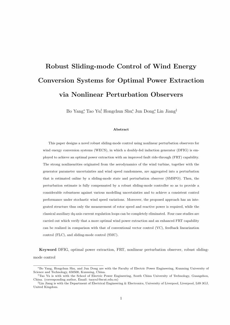
A stochastic wind speed variation is tested to examine the control performance of the proposed approach,226

which starts from 8 m/s and gradually reaches to 12 m/s, as demonstrated by Fig. 5. The system227

responses are provided in Fig. 6, from which it can be clearly observed that POSMC is able to achieve the228

least oscillations of rotor speed error and reactive power thanks to the online perturbation compensation.229

Additionally, its power coefficient is the closest to the optimum thus the wind energy can be optimally230

15

0 5 10 15 20 25 30Time (s)

-10

-8

-6

-4

-2

0

2

4

6

8

Act

ive

pow

er P

e (p.

u.)

VCFLCSMCPOSMC

19 20 21 22 23

-8

-6

-4

-2

0

2

4

6

8

0 5 10 15 20 25 30Time (s)

0.426

0.428

0.43

0.432

0.434

0.436

0.438

0.44

Pow

er c

oeff

icie

nt C

p (p.

u.)

VCFLCSMCPOSMC

20 21 22 23

0.432

0.433

0.434

0.435

0.436

0.437

0.438

0 5 10 15 20 25 30Time (s)

-0.1

-0.08

-0.06

-0.04

-0.02

0

0.02

Rot

or s

peed

err

or ω

err (

p.u.

)

VCFLCSMCPOSMC

20 21 22 23

-0.08

-0.06

-0.04

-0.02

0

0 5 10 15 20 25 30Time (s)

-2

-1.5

-1

-0.5

0

0.5

1

Rea

ctiv

e po

wer

err

or Q

err (

p.u.

)

VCFLCSMCPOSMC

14.5 15 15.5 16 16.5 17 17.5-1

-0.5

0

0.5

Figure 4: MPPT performance to a series of step change of wind speed from 8 m/s to 12 m/s.

16

0 5 10 15Time (s)

8

9

10

11

12

Win

d sp

eed

vw

ind

(m/s

)

Figure 5: The tested random wind speed variation from 8 m/s to 12 m/s.

extracted under random wind speed variations.231

5.3 FRT performance232

With the rapidly ever-growing integration of WECS into the main power grid, it often requires that233

WECS can realize FRT when the power grid voltage is temporarily reduced due to a fault or a sudden234

load change occurred in the power grid, or can even address the generator to stay operational and not235

disconnect from the power grid during and after the voltage drop [39,40]. A 625 ms voltage dip staring at236

t=1 s from nominal value to 0.3 p.u. and restores to 0.9 p.u. is applied [41], while the system responses237

are presented by Fig. 7. One can definitely find that POSMC is able to effectively suppress the power238

oscillations and maintain the largest wind power extraction during FRT, while VC requires the longest239

time to restore the system from such harmful contingencies.240

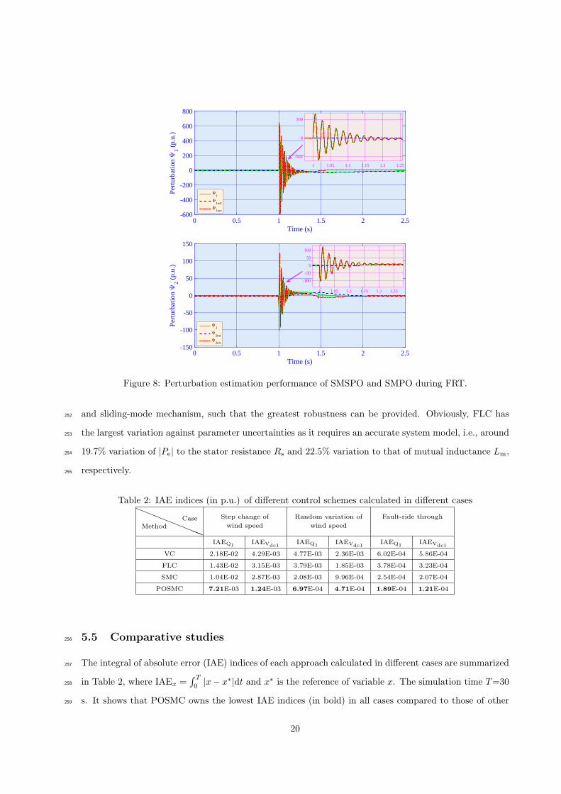
Lastly, the estimation performance of perturbation observers during the FRT has also been carefully241

monitored, as shown in Fig. 8. It gives that the perturbations can be rapidly estimated in around 250242

ms while the relative high-frequency oscillations emerged in the initial phase is due to the discontinuity243

of power grid voltage and sliding-mode mechanism caused in perturbation observer loop.244

5.4 System robustness with parameter uncertainties245

A series of plant-model mismatches of stator resistance Rs and mutual inductance Lm with ±20% un-246

certainties are undertaken to evaluate the robustness of POSMC, in which a 0.25 p.u. voltage drop at247

power grid is tested while the peak value of total active power |Pe| is recorded for a clear comparison. It248

presents from Fig. 9 that the variation of |Pe| obtained by POSMC is the smallest among all approach-249

es, i.e., around 2.3% variation of |Pe| to the stator resistance Rs and 1.4% variation to that of mutual250

inductance Lm, respectively. This is because of its elegant merits of the full perturbation compensation251

17

0 5 10 15Time (s)

-0.4

-0.2

0

0.2

0.4

0.6

0.8

1

1.2

Act

ive

pow

er P

e (p.

u.)

VCFLCSMCPOSMC

4 4.5 5 5.5 6 6.5 7 7.5 8 8.5

-0.4

-0.2

0

0.2

0.4

0.6

0.8

0 5 10 15Time (s)

0.4366

0.4368

0.437

0.4372

0.4374

0.4376

0.4378

0.438

0.4382

0.4384

Pow

er c

oeff

icie

nt C

p (p.

u.)

VCFLCSMCPOSMC

1 1.5 2 2.5 3 3.5 4 4.5 5

0.4366

0.4368

0.437

0.4372

0.4374

0.4376

0.4378

0.438

0.4382

0 5 10 15Time (s)

-0.035

-0.03

-0.025

-0.02

-0.015

-0.01

-0.005

0

0.005

Rot

or s

peed

err

or ω

err (

p.u.

)

VCFLCSMCPOSMC

5 5.5 6 6.5 7 7.5 8 8.5 9 9.5 10

-16

-14

-12

-10

-8

-6

-4

-2

0

2

4×10-3

0 5 10 15Time (s)

-0.06

-0.05

-0.04

-0.03

-0.02

-0.01

0

0.01

0.02

0.03

Rea

ctiv

e po

wer

err

or Q

err (

p.u.

)

VCFLCSMCPOSMC

5 6 7 8 9

-0.01

0

0.01

0.02

Figure 6: MPPT performance to a random variation of wind speed from 8 m/s to 12 m/s.

18

0 0.5 1 1.5 2 2.5 3 3.5 4Time (s)

-1

-0.5

0

0.5

1

1.5

2

2.5

Act

ive

pow

er P

e (p.

u.)

VCFLCSMCPOSMC

1 1.2 1.4 1.6 1.8 2

-0.5

0

0.5

1

1.5

2

0 0.5 1 1.5 2 2.5 3 3.5 4Time (s)

0.4376

0.4377

0.4378

0.4379

0.438

0.4381

0.4382

0.4383

Pow

er c

oeff

icie

nt C

p (p.

u.)

VCFLCSMCPOSMC

1 1.2 1.4 1.6 1.8 2 2.2

0.4377

0.43775

0.4378

0.43785

0.4379

0.43795

0.438

0.43805

0.4381

0.43815

0.4382

0 0.5 1 1.5 2 2.5 3 3.5 4Time (s)

-0.015

-0.01

-0.005

0

0.005

0.01

0.015

0.02

0.025

0.03

Rot

or s

peed

err

or ω

err (

p.u.

)

VCFLCSMCPOSMC

1 1.2 1.4 1.6 1.8 2 2.2

-0.01

-0.005

0

0.005

0.01

0.015

0.02

0.025

0 0.5 1 1.5 2 2.5 3 3.5 4Time (s)

-1

-0.5

0

0.5

1

1.5

2

2.5

3

3.5

4

Rea

ctiv

e po

wer

err

or Q

err (

p.u.

)

VCFLCSMCPOSMC

1 1.1 1.2 1.3 1.4 1.5 1.6 1.7 1.8

-0.5

0

0.5

1

1.5

2

2.5

3

3.5

Figure 7: System responses under FRT (a 625 ms voltage dip staring at t=1 s from nominal value to 0.3p.u. and restores to 0.9 p.u.).

19

0 0.5 1 1.5 2 2.5Time (s)

-600

-400

-200

0

200

400

600

800

Pert

urba

tion Ψ

1 (p.

u.)

Ψ1

Ψ1est

Ψ1err

1 1.05 1.1 1.15 1.2 1.25

-500

0

500

0 0.5 1 1.5 2 2.5Time (s)

-150

-100

-50

0

50

100

150

Pert

urba

tion Ψ

2 (p.

u.)

Ψ2

Ψ2est

Ψ2err

1 1.05 1.1 1.15 1.2 1.25

-100

-50

0

50

100

Figure 8: Perturbation estimation performance of SMSPO and SMPO during FRT.

and sliding-mode mechanism, such that the greatest robustness can be provided. Obviously, FLC has252

the largest variation against parameter uncertainties as it requires an accurate system model, i.e., around253

19.7% variation of |Pe| to the stator resistance Rs and 22.5% variation to that of mutual inductance Lm,254

respectively.255

Table 2: IAE indices (in p.u.) of different control schemes calculated in different casesaaaaaaaaMethod

Case Step change of

wind speed

Random variation of

wind speed

Fault-ride through

IAEQ1 IAEVdc1IAEQ1 IAEVdc1

IAEQ1 IAEVdc1

VC 2.18E-02 4.29E-03 4.77E-03 2.36E-03 6.02E-04 5.86E-04

FLC 1.43E-02 3.15E-03 3.79E-03 1.85E-03 3.78E-04 3.23E-04

SMC 1.04E-02 2.87E-03 2.08E-03 9.96E-04 2.54E-04 2.07E-04

POSMC 7.21E-03 1.24E-03 6.97E-04 4.71E-04 1.89E-04 1.21E-04

5.5 Comparative studies256

The integral of absolute error (IAE) indices of each approach calculated in different cases are summarized257

in Table 2, where IAEx =∫ T

0|x− x∗|dt and x∗ is the reference of variable x. The simulation time T=30258

s. It shows that POSMC owns the lowest IAE indices (in bold) in all cases compared to those of other259

20

0.8 0.825 0.85 0.875 0.9 0.925 0.95 0.975 1.0 1.025 1.05 1.075 1.1 1.125 1.15 1.175 1.2%Rs plant-model mismatch

1

1.05

1.1

1.15

1.2

1.25

Pea

k v

alue

|Pe|

(p.u

.)

POSMCSMCFLCVC

0.85 0.875 0.9 0.925 0.95

1.04

1.05

1.06

1.07

1.08

1.09

1.1

0.8 0.825 0.85 0.875 0.9 0.925 0.95 0.975 1.0 1.025 1.05 1.075 1.1 1.125 1.15 1.175 1.2%L

m Plant-model mismatch

1

1.05

1.1

1.15

1.2

1.25

1.3

Pea

k v

alue

|Pe|

(p.u

.)

POSMCSMCFLCVC

0.85 0.875 0.9 0.925 0.95

1.06

1.08

1.1

1.12

Figure 9: Peak value of active power |Pe| obtained under a 0.25 p.u. voltage drop at power grid with 20%variation of the stator resistance Rs and mutual inductance Lm of different approaches, respectively.

methods. In particular, its IAEQ1 obtained in random variation of wind speed is merely 33.51%, 18.39%,260

and 14.61% to that of SMC, FLC, and VC, respectively; Additionally, its IAEVdc1obtained in voltage261

drop at power grid is just 58.45%, 37.46%, and 20.65% to that of SMC, FLC, and VC, respectively.262

The overall control efforts of different controllers needed in three cases are given in Fig. 10. One can263

easily conclude that the overall control efforts of POSMC are the least in all cases except of FRT, this is264

resulted from its merits that the over-conservativeness of control efforts is only involved in the observer265

loop and excluded from the controller loop. Therefore, POSMC outperforms other methods with greater266

robustness enhancement as well as more reasonable control efforts.267

6 Conclusions268

This paper proposes a robust sliding-mode controller scheme called POSMC to achieve an optimal pow-269

er extraction of DFIG in various operation conditions. A perturbation is firstly defined to aggregate270

the wind turbine nonlinearities, generator parameter uncertainties, and wind speed randomness, which271

is then rapidly estimated by nonlinear perturbation observers and fully compensated by POSMC, so272

that a consistent and robust control performance under different operation conditions can be achieved.273

21

Figure 10: Comparison of control efforts (in p.u.) of different controllers required in three cases.

Simulation results have demonstrated that POSMC can optimally extract the wind energy during wind274

speed variations and effectively suppress the power oscillations during FRT, together with suitable control275

efforts thanks to the perturbation compensation.276

Compared to other typical nonlinear robust approaches, POSMC can be readily implemented in277

practice as it only requires the measurement of rotor speed (by an additional rotor speed measuring278

apparatus) and reactive power (read directly from current power measurement platform), hence the279

construction costs of measurement apparatus is quite low. Moreover, as POSMC is a decentralized280

control scheme, no central controller is needed in the face of large-scale wind farms.281

Appendix282

System parameters [7, 11, 33]:283

ωb = 100π rad/s, ωs = 1.0 p.u., ωr base = 1.29, vs nom = 1.0 p.u..284

DFIG parameters:285

Prated = 5 MW, Rs = 0.005 p.u., Rr = 1.1Rs, Lm = 4.0 p.u., Lss = 1.01Lm, Lrr = 1.005Lss, L′s =286

Lss − L2m/Lrr, Tr = Lrr/Rr, R1 = Rs +R2, R2 = (Lm/Lrr)

2Rr.287

Wind turbine parameters:288

ρ = 1.225 kg/m3, R = 58.59 m2, vwind nom = 12 m/s, λopt = 6.325, Hm = 4.4 s, D = 0 p.u..289

Acknowledgements290

The authors gratefully acknowledge the support of National Basic Research Program of China (973291

Program: 2013CB228205), National Natural Science Foundation of China (51477055,51667010), Yunnan292

22

Provincial Talents Training Program (KKSY201604044), and Scientific Research Foundation of Yunnan293

Provincial Department of Education (KKJB201704007).294

References295

[1] Hooper T., Beaumont N., and Hattam C. ‘The implications of energy systems for ecosystem services:296

A detailed case study of offshore wind’, Renewable and Sustainable Energy Reviews, 70, 230-241297

(2017).298

[2] Matteo M., Riccardo M., Vincenzo D., and Riccardo A. ‘A new model for environmental and299

economic evaluation of renewable energy systems: The case of wind turbines’, Applied Energy, 189,300

739-752 (2017).301

[3] Li S. H., Haskew T. A., Williams K. A., and Swatloski R. P. ‘Control of DFIG wind turbine with302

direct-current vector control configuration’, IEEE Transactions on Sustainable Energy, 3(1), 1-11303

(2012).304

[4] Song D., Yang J., Cai Z., Dong M., Su M., and, Wang Y. ‘Wind estimation with a non-standard305

extended Kalman filter and its application on maximum power extraction for variable speed wind306

turbines’, Applied Energy, 190, 670-685 (2017).307

[5] Gilmanur R. and Mohd H. A., ‘Fault ride through capability improvement of DFIG based wind farm308

by fuzzy logic controlled parallel resonance fault current limiter’, Electric Power Systems Research,309

146, 1-8 (2017).310

[6] Heri S., Arif M., et al. ‘Optimal controller for doubly fed induction generator (DFIG) using differ-311

ential evolutionary algorithm (DE)’, 2015 International seminar on intelligent technology and its312

applications, p. 159-164 (2015).313

[7] Yang B., Zhang X. S., Yu T., Shu H. C., and Fang Z. H. ‘Grouped grey wolf optimizer for maximum314

power point tracking of doubly-fed induction generator based wind turbine’, Energy Conversion and315

Management, 133, 427-443 (2017).316

[8] Delgarm N., Sajadi B., Kowsary F., and Delgarm S., ‘Multi-objective optimization of the building317

energy performance: A simulation-based approach by means of particle swarm optimization (PSO)’,318

Applied Energy, 170, 293-303 (2016).319

23

[9] Wieczorek M. and Lewandowski M. ‘A mathematical representation of an energy management320

strategy for hybrid energy storage system in electric vehicle and real time optimization using a321

genetic algorithm’, Applied Energy, 192, 222-233 (2017).322

[10] Sachez-Lozano J. M., Garcia-Cascales M. S., and Lamata M. T. ‘GIS-based onshore wind farm site323

selection using Fuzzy Multi-Criteria Decision Making methods. Evaluating the case of Southeastern324

Spain’, Applied Energy, 171, 86-102 (2016).325

[11] Yang B., Jiang L., Wang L., Yao W., and Wu Q. H. ‘Nonlinear maximum power point tracking326

control and modal analysis of DFIG based wind turbine’, International Journal of Electrical Power327

and Energy Systems, 74, 429-436 (2016).328

[12] Gayen P. K., Chatterjee D., and Goswami S. K. ‘Stator side active and reactive power control329

with improved rotor position and speed estimator of a grid connected DFIG (doubly-fed induction330

generator)’, Energy, 89, 461-472 (2015).331

[13] Errouissi R., Al-Durra A., Muyeen S. M., Leng S., and Blaabjerg F. ‘Offset-free direct power control332

of DFIG under continuous-time model predictive control’, IEEE Transactions on Power Electronics,333

32(3), 2265-2277 (2017).334

[14] Taveiros F. E. V., Barros L. S., and Costa F. B. ‘Back-to-back converter state-feedback control of335

DFIG (doubly-fed induction generator)-based wind turbines’, Energy, 89, 896-906 (2015).336

[15] Phan D. C. and Yamamoto S. ‘Rotor speed control of doubly fed induction generator wind turbines337

using adaptive maximum power point tracking’, Energy, 111, 377-388 (2016).338

[16] Badre B., Mohammed K., Ahmed L., Mohammed T., and Aziz D. ‘Observer backstepping control339

of DFIG-Generators for wind turbines variable-speed: FPGA-based implementation’, Renewable340

Energy, 81, 903-917 (2015).341

[17] Guo W. T., Liu F., Si J., He D., Harley R., and Mei S. W. ‘Approximate dynamic programming342

based supplementary reactive power control for DFIG wind farm to enhance power system stability’,343

Neurocomputing, 170, 417-427 (2015).344

[18] Maissa F., Oscar B., and Lassaad S. ‘A new maximum power point method based on a sliding mode345

approach for solar energy harvesting’, Applied Energy, 185, 1185-1198 (2017).346

24

[19] Saad N. H., Sattar A. A., and Mansour A. E. M. ‘Low voltage ride through of doubly-fed induction347

generator connected to the grid using sliding mode control strategy’, Renewable Energy, 80, 583-594348

(2015).349

[20] Benbouzid M., Beltran B., Amirat Y., Yao G., Han J. G., and Mangel H. ‘Second-order slid-350

ing mode control for DFIG-based wind turbines fault ride-through capability enhancement’, ISA351

Transactions, 53, 827-833, (2014).352

[21] Soufi Y., Kahla S., and Bechouat M. ‘Particle swarm optimization based sliding mode control353

of variable speed wind energy conversion system’, International Journal of Hydrogen Energy, 41,354

20956-20963 (2016).355

[22] Li S. Z., Wang H. P., Tian Y., Aitouch A., and Klein J. ‘Direct power control of DFIG wind turbine356

systems based on an intelligent proportional-integral sliding mode control’, ISA Transactions, 64,357

431-439 (2016).358

[23] Ebrahimkhani S. ‘Robust fractional order sliding mode control of doubly-fed induction generator359

(DFIG)-based wind turbines’, ISA Transactions, 63, 343-354 (2016).360

[24] Yang B., Jiang L., Yao W., and Wu Q. H. ‘Perturbation estimation based coordinated adaptive361

passive control for multimachine power systems’, Control Engineering Practice, 44, 172-192 (2015).362

[25] Tohidi A., Hajieghrary H., and Hsieh M. A. ‘Adaptive disturbance rejection control scheme for363

DFIG-based wind turbine: theory and experiments’, IEEE Transactions on Industry Applications,364

52(3), 2006-2015 (2016).365

[26] Tang Y. M., Bai Y., Huang C. Z., and Du B. ‘Linear active disturbance rejection-based load366

frequency control concerning high penetration of wind energy’, Energy Conversion and Managemen,367

95, 259-271, (2015).368

[27] Liu Y., Wu Q. H., Zhou X. X., and Jiang L. ‘Perturbation observer based multiloop control for the369

DFIG-WT in multimachine power system’, IEEE Transactions on Power Systems, 29(6), 2905-2915370

(2014).371

[28] Zhang J., Liu X., Xia Y., Zuo Z., and Wang Y. ‘Disturbance observer-based integral sliding-mode372

control for systems with mismatched disturbances’, IEEE Transactions on Industrial Electronics,373

63(11), 7040-7048 (2016).374

25

[29] Yang B., Sang Y. Y., Shi K., Yao W., Jiang L., and Yu T. ‘Design and real-time implementation375

of perturbation observer based sliding-mode control for VSC-HVDC systems’, Control Engineering376

Practice, 56, 13-26 (2016).377

[30] Mi Y., Fu Y., Li D. D., Wang C. S., Loh P. C., and Wang P. ‘The sliding mode load frequency378

control for hybrid power system based on disturbance observer’, International Journal of Electrical379

Power and Energy Systems, 74, 446-452 (2016).380

[31] Lee Y., Kim S. H., and Chung C. C. ‘Integral sliding mode control with a disturbance observer for381

next-generation servo track writing’, Mechatronics, 40, 106-114 (2016).382

[32] Rigatos G., Siano P., Zervos N., and Cecati C. ‘Control and disturbances compensation for doubly383

fed induction generators using the derivative-free nonlinear kalman filter’, IEEE Transactions on384

Power Electronics, 30(10), 5532-5547 (2015).385

[33] Fei M. and Pal B. ‘Modal analysis of grid-connected doubly fed induction generators’, IEEE Trans-386

actions on Energy Conversion, 22, 728-736 (2007).387

[34] Qiao W. ‘Dynamic modeling and control of doubly fed induction generators driven by wind tur-388

bines’, Power Systems Conference & Exposition, p. 1-8 (2009).389

[35] Rezaeihaa A., Kalkmana I., and Blocken B. ‘Effect of pitch angle on power performance and aero-390

dynamics of a vertical axis wind turbine’, Applied Energy, 197, 132-150 (2017).391

[36] Song D. R., Yang J., Cai Z. L., Dong M., Su M., and Wang Y. H. ‘Wind estimation with a non-392

standard extended Kalman filter and its application on maximum power extraction for variable393

speed wind turbines’, Applied Energy, 190, 670-685 (2017).394

[37] Sanjoy R. ‘Performance prediction of active pitch-regulated wind turbine with short duration vari-395

ations in source wind’, Applied Energy, 114, 700-708 (2014).396

[38] Juan R., Edgar L., Vicente V., David C., Ramon A., and Luis E. ‘Current-sensorless control of an397

SPWM H-Bridge-based PFC rectifier designed considering voltage sag condition’, Electric Power398

Systems Research 130, 181-191 (2016).399

[39] Liu J., Wen J. Y., Yao W., and Long Y. ‘Solution to short-term frequency response of wind farms400

by using energy storage systems’, IET Renewable Power Generation 10(5), 669-678 (2016).401

26

[40] Liao S. W., Yao W., Han X. N., Wen J. Y., and Cheng S. J. ‘Chronological operation simulation402

framework for regional power system under high penetration of renewable energy using meteoro-403

logical data’, Applied Energy 203, 816-828 (2017).404

[41] Yao W., Jiang L., Wen J. Y., Wu Q. H., and Cheng S. J. ‘Wide-area damping controller for power405

system inter-area oscillations: a networked predictive control approach’, IEEE Transactions on406

Control Systems Technology 23(1), 27-36 (2015).407

27