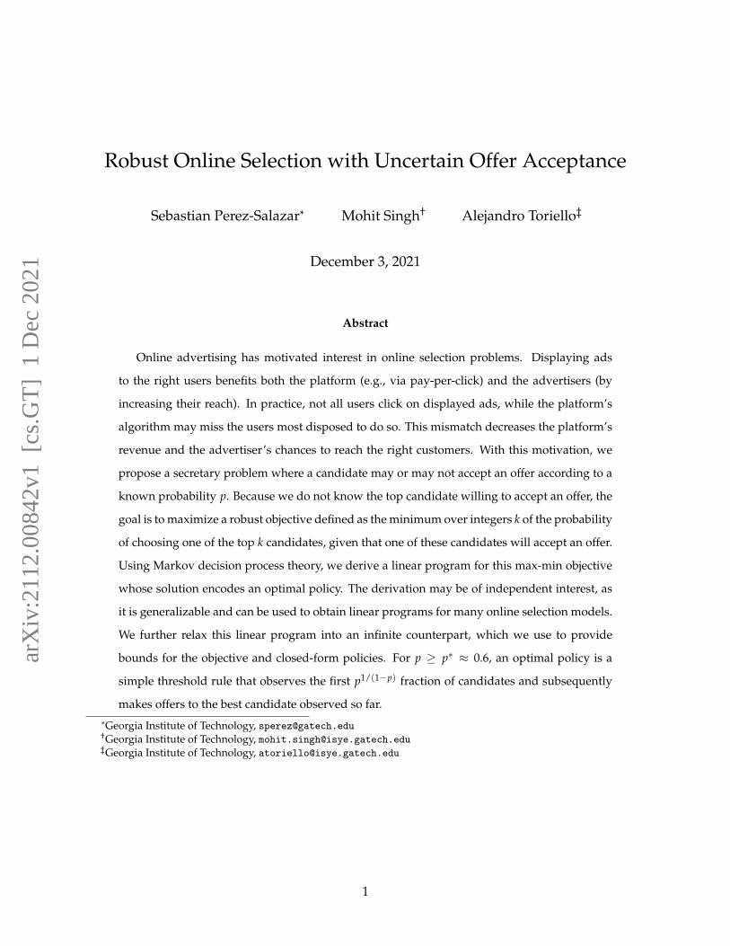
Robust Online Selection with Uncertain Offer Acceptance

Sebastian Perez-Salazar* Mohit Singh† Alejandro Toriello‡

December 3, 2021

Abstract

Online advertising has motivated interest in online selection problems. Displaying ads

to the right users benefits both the platform (e.g., via pay-per-click) and the advertisers (by

increasing their reach). In practice, not all users click on displayed ads, while the platform’s

algorithm may miss the users most disposed to do so. This mismatch decreases the platform’s

revenue and the advertiser’s chances to reach the right customers. With this motivation, we

propose a secretary problem where a candidate may or may not accept an offer according to a

known probability p. Because we do not know the top candidate willing to accept an offer, the

goal is to maximize a robust objective defined as the minimum over integers k of the probability

of choosing one of the top k candidates, given that one of these candidates will accept an offer.

Using Markov decision process theory, we derive a linear program for this max-min objective

whose solution encodes an optimal policy. The derivation may be of independent interest, as

it is generalizable and can be used to obtain linear programs for many online selection models.

We further relax this linear program into an infinite counterpart, which we use to provide

bounds for the objective and closed-form policies. For p ≥ p∗ ≈ 0.6, an optimal policy is a

simple threshold rule that observes the first p1/(1−p) fraction of candidates and subsequently

makes offers to the best candidate observed so far.

*Georgia Institute of Technology, sperez@gatech.edu†Georgia Institute of Technology, mohit.singh@isye.gatech.edu‡Georgia Institute of Technology, atoriello@isye.gatech.edu

1

arX

iv:2

112.

0084

2v1

[cs

.GT

] 1

Dec

202

1

1 Introduction

The growth of online platforms has spurred renewed interest in online selection problems, auc-

tions and stopping problems (Edelman et al., 2007; Lucier, 2017; Devanur and Hayes, 2009; Alaei

et al., 2012; Mehta et al., 2014). Online advertising has particularly benefited from developments

in these areas. As an example, in 2005 Google reported about $6 billion in revenue from adver-

tising, roughly 98% of the company’s total revenue at that time; in 2020, Google’s revenue from

advertising grew to almost $147 billion. Thanks in part to the economic benefits of online adver-

tisement, internet users can freely access a significant amount of online content and many online

services.

Targeting users is crucial for the success of online advertising. Studies suggest that targeted cam-

paigns can double click-through rates in ads (Farahat and Bailey, 2012) despite the fact that internet

users have acquired skills to navigate the web while ignoring ads (Cho and Cheon, 2004; Dreze

and Hussherr, 2003). Therefore, it is natural to expect that not every displayed ad will be clicked

on by a user, even if the user likes the product on the ad, whereas the platform and advertiser’s

revenue depend on this event (Pujol et al., 2015). An ignored ad misses the opportunity of be-

ing displayed to another user willing to click on it and decreases the return on investment (ROI)

for the advertiser, especially in cases where the platform uses methods like pay-for-impression

to charge the advertisers. At the same time, the ignored ad uses the space of another, possibly

more suitable ad for that user. In this work, we take the perspective of a single ad, and we aim to

understand the right time to begin displaying the ad to users as a function of the ad’s probability

of being clicked.

Recent works have addressed this uncertainty from a full-information perspective (Mehta et al.,

2014; Goyal and Udwani, 2020), where user’s valuations over the ads are known in hindsight.

However, in many e-commerce applications it is unrealistic to assume access to complete infor-

mation, as users may approach the platform sequentially. Platforms that depend at least partially

on display advertisement for revenue observe sequential user visits and need to irrevocably de-

cide when to display an ad. If a platform displays an ad too soon, it risks not being able to learn

users’ true preferences, while spending too much time learning preferences risks missing a good

2

opportunity to display an ad. Designing efficient policies for displaying ads to users is key for

large internet companies such as Google and Meta, as well as for small businesses advertising

their products in these platforms.

We model the interaction between the platform and the users using a general online selection

problem. We refer to it as the secretary problem with uncertain acceptance (SP-UA for short). Using

the terminology of candidate and decision maker, the general interaction is as follows:

1. Similar to other secretary problems, a finite sequence of candidates of known length arrives

online, in a random order. In our motivating application, candidates represent platform users.

2. Upon an arrival, the decision maker (DM) is able to assess the quality of a candidate compared

to previously observed candidates and has to irrevocably decide whether to extend an offer to

the candidate or move on to the next candidate. This captures the online dilemma the platform

faces: the decision of displaying an ad to a user is based solely on information obtained up to

this point.

3. When the DM extends an offer, the candidate accepts with a known probability p ∈ (0, 1], in

which case the process ends, or turns down the offer, in which case the DM moves on to the

next candidate. This models the users, who can click on the ad or ignore it.

4. The process continues until either a candidate accepts an offer or the DM has no more candi-

dates to assess.

A DM that knows in advance that at least one of the top k candidates is willing to accept the offer

would like to maximize the probability of making an offer to one of these candidates. In reality, the

DM does not know k; hence, the best she can do is maximize the minimum of all these scenario-

based probabilities. We call the minimum of these scenario-based probabilities the robust ratio

and our max-min objective the optimal robust ratio (see Subsection 1.2 for a formal description).

Suppose that the DM implements a policy that guarantees a robust ratio γ ∈ (0, 1]. This implies

the DM will succeed with probability at least γ in obtaining a top k candidate, in any scenario

where a top k candidate is willing to accept the DM’s offer. This is an ex-ante guarantee when the

DM knows the odds for each possible scenario, but the policy is independent of k and offers the

3

same guarantee for any of these scenarios. Moreover, if the DM can assign a numerical valuation

to the candidates, a policy with robust ratio γ can guarantee a factor at least γ of the optimal

offline value. Tamaki (1991) also studies the SP-UA and considers the objective of maximizing

the probability of selecting the best candidate willing to accept the offer. Applying his policy to

value settings can also guarantee an approximation factor of the optimal offline cost; however, the

policy with the optimal robust ratio attains the largest approximation factor of the optimal offline

value among rank-based policies (see Proposition 1).

Our contributions (1) We propose a framework and a robust metric to understand the interac-

tion between a DM and competing candidates, when candidates can reject the DM’s offer. (2) We

state a linear program (LP) that computes the optimal robust ratio and the best strategy. We pro-

vide a general methodology to deduce our LP, and this technique is generalizable to other online

selection problems. (3) We provide bounds for the optimal robust ratio as a function of the proba-

bility of acceptance p ∈ (0, 1]. (4) We present a family of policies based on simple threshold rules;

in particular, for p ≥ p∗ ≈ 0.594, the optimal strategy is a simple threshold rule that skips the first

p1/(1−p) fraction of candidates and then makes offers to the best candidate observed so far. We

remark that as p→ 1 we recover the guarantees of the standard secretary problem and its optimal

threshold strategy. (5) Finally, for the setting where candidates also have non-negative numerical

values, we show that our solution is the optimal approximation among rank-based algorithms

of the optimal offline value, where the benchmark knows the top candidate willing to accept the

offer. The optimal approximation factor equals the optimal robust ratio.

In the remainder of the section, we discuss additional applications of SP-UA, give a formal de-

scription of the problem, and summarize our technical contributions and results.

1.1 Additional applications

SP-UA captures the inherent unpredictability in online selection, as other secretary problems do,

but also the uncertainty introduced by the possibility of candidates turning down offers. Although

our main motivation is online advertisement, SP-UA is broadly applicable; the following are ad-

ditional concrete examples.

4

Data-driven selection problems When selling an item in an auction, buyers’ valuations are typ-

ically unknown beforehand. Assuming valuations follow a common distribution, the aim is to

sell the item at the highest price possible; learning information about the distribution is crucial

for this purpose. In particular auction settings, the auctioneer may be able to sequentially observe

the valuations of potential buyers, and can decide in an online manner whether to sell the item or

continue observing valuations. Specifically, the auctioneer decides to consider the valuation of a

customer with probability p and otherwise the auctioneer moves on to see the next buyer’s val-

uation. The auctioneer’s actions can be interpreted as an exploration-exploitation process, which is

often found in bandit problems and online learning (Cesa-Bianchi and Lugosi, 2006; Hazan, 2019;

Freund and Schapire, 1999). This setting is also closely related to data-driven online selection and

the prophet inequality problem (Campbell and Samuels, 1981; Kaplan et al., 2020; Kertz, 1986);

some of our results also apply in these models (see Section 6).

Human resource management As its name suggests, the original motivation for the secretary

problem is in hiring for a job vacancy. Glassdoor reported in 2015 that each job posting receives

on average 250 resumes. From this pool of resumes, only a small fraction of candidates are called

for an interview. Screening resumes can be a time-consuming task that shift resources away from

the day-to-day job in Human Resources. Since the advent of the internet, several elements of

the hiring process can be partially or completely automated; for example, multiple vendors offer

automated resume screening (Raghavan et al., 2019), and machine learning algorithms can score

and rank job applicants according to different criteria. Of course, a highly ranked applicant may

nevertheless turn down a job offer. Although we consider the rank of a candidate as an abso-

lute metric of their capacities, in reality, resume screening may suffer from different sources of

bias (Salem and Gupta, 2019), but addressing this goes beyond our scope. See also Smith (1975);

Tamaki (1991); Vanderbei (2012) for classical treatments. Similar applications include apartment

hunting (Bruss, 1987; Cowan and Zabczyk, 1979; Presman and Sonin, 1973), among others.

1.2 Problem formulation

A problem instance is given by a fixed probability p ∈ (0, 1] and the number of candidates n. These

are ranked by a total order, 1 ≺ 2 ≺ · · · ≺ n, with 1 being the best or highest-ranked candidate.

5

The candidate sequence is given by a random permutation π = (R1, . . . , Rn) of [n] .= {1, 2, . . . , n},

where any permutation is equally likely. At time t, the DM observes the partial rank rt ∈ [t] of the

t-th candidate in the sequence compared to the previous t− 1 candidates. The DM either makes

an offer to the t-th candidate or moves on to the next candidate, without being able to make an

offer to the t-th candidate ever again. If the t-th candidate receives an offer from the DM, she

accepts the offer with probability p, in which case the process ends. Otherwise, if the candidate

refuses the offer (with probability 1− p), the DM moves on to the next candidate and repeats the

process until she has exhausted the sequence. A candidate with rank in [k] is said to be a top k

candidate. The goal is to design a policy that maximizes the probability of extending an offer to a

highly ranked candidate that will accept the DM’s offer. To measure the quality of a policy P , we

use the robust ratio

γP = γP (p) = mink=1,...,n

P(P selects a top k candidate, candidate accepts offer)P(At least one of the top k candidates accepts offer)

. (1)

The ratio inside the minimization operator equals the probability that the policy successfully se-

lects a top k candidate given that some top k candidate will accept an offer. If we consider the

game where an adversary knows in advance if any of the top k candidates will accept the offer,

the robust ratio γP captures the scenario where the DM that follows policy P has the worst per-

formance. When p = 1, the robust ratio γP equals the probability of selecting the highest ranked

candidate, thus we recover the standard secretary problem. The goal is to find a policy that maxi-

mizes this robust ratio, γ∗n.= supP γP . We say that the policy P is γ-robust if γ ≤ γP .

1.3 Our technical contributions

Recent works have studied secretary models using linear programming (LP) methods (Buchbinder

et al., 2014; Chan et al., 2014; Correa et al., 2020; Dutting et al., 2021). We also give an LP formu-

lation that computes the best robust ratio and the optimal policy for our model. Whereas these

recent approaches derive an LP formulation using ad-hoc arguments, our first contribution is to

provide a general framework to obtain LP formulations that give optimal bounds and policies for

different variants of the secretary problem. The framework is based on Markov decision process

6

(MDP) theory (Altman, 1999; Puterman, 2014). This is surprising since early literature on secre-

tary problem used MDP techniques, e.g. Dynkin (1963); Lindley (1961), though typically not LP

formulations. In that sense, our results connect the early algorithms based on MDP methods with

the recent literature based on LP methods. Specifically, we provide a mechanical way to obtain an

LP using a simple MDP formulation (Section 4). Using this framework, we present a structural

result that completely characterizes the space of policies for the SP-UA:

Theorem 1 Any policy P for the SP-UA can be represented as a vector in the set

POL =

{(x, y) ≥ 0 : xt,s + yt,s =

1t

t−1

∑σ=1

(yt−1,σ + (1− p)xt−1,σ) , ∀t > 1, s ∈ [t], x1,1 + y1,1 = 1

}.

Conversely, any vector (x, y) ∈ POL represents a policy P . The policy P makes an offer to the first candi-

date with probability x1,1 and to the t-th candidate with probability txt,s/(

∑t−1σ=1 yt−1,σ + (1− p)xt−1,σ

)if the t-th candidate has partial rank rt = s.

The variables xt,s represent the probability of reaching candidate t and making an offer to that

candidate when that candidate has partial rank s ∈ [t]. Likewise, the variables yt,s represent the

probability of reaching candidate t and moving on to the next candidate when the t-th candidate’s

partial rank is s ∈ [t]. We note that although the use of LP formulations in MDP is a somewhat

standard technique, see e.g. Puterman (2014), the recent literature in secretary problems and re-

lated online selection models does not appear to make an explicit connection between LP’s used

in analysis and the underlying MDP formulation.

Problems solved via MDP can typically be formulated as reward models, where each action taken

by the DM generates some immediate reward. Objectives in classical secretary problems fit in this

framework, as the reward (e.g. the probability of selecting the top candidate) depends only on

the current state (the number t of observed candidates so far and the current candidate’s partial

rank rt = s), and on the DM’s action (make an offer or not); see Section 4.1 for an example. Our

robust objective, however, cannot be easily written as a reward depending only on rt = s. Thus,

we split the analysis into two stages. In the first stage, we deal with the space of policies and

formulate an MDP for our model with a generic utility function. The feasible region of this MDP’s

LP formulation corresponds to POL and is independent of the utility function chosen; therefore, it

7

characterizes all possible policies for the SP-UA. In the second stage, we use the structural result

in Theorem 1 to obtain a linear program that finds the largest robust ratio.

Theorem 2 The best robust ratio γ∗n for the SP-UA equals the optimal value of the linear program

(LP)n,p

maxx≥0

γ

s.t.

xt,s ≤1t

(1− p

t−1

∑τ=1

τ

∑σ=1

xτ,σ

)∀t ∈ [n], s ∈ [t]

γ ≤ p1− (1− p)k

n

∑t=1

t

∑s=1

xt,s P(Rt ≤ k | rt = s) ∀k ∈ [n],

where P(Rt ≤ k | rt = s) = ∑k∧(n−t+s)i=s (i−1

s−1)(n−it−s)/(

nt) is the probability the t-th candidate is ranked in

the top k given that her partial rank is s.

Moreover, given an optimal solution (x∗, γ∗n) of (LP)n,p, the (randomized) policy P∗ that at state (t, s)

makes an offer with probability tx∗t,s/(

1− p ∑t−1τ=1 ∑τ

σ=1 x∗τ,σ

)is γ∗n-robust.

We show that γP can be written as the minimum of n linear functions on the x variables in POL,

where these variables correspond to a policy’s probability of making an offer in a given state.

Thus our problem can be written as the maximum of a concave piecewise linear function over

POL, which we linearize with the variable γ. By projecting the feasible region onto the (x, γ)

variables we obtain (LP)n,p.

As a byproduct of our analysis via MDP, we show that γ∗n is non-increasing in n for fixed p ∈ (0, 1]

(Lemma 1), and thus limn→∞ γ∗n = γ∗∞ exists. We show that this limit corresponds to the optimal

value of an infinite version of (LP)n,p from Theorem 2, where n tends to infinity and we replace

sums at time t with integrals (see Section 5). This allows us to show upper and lower bounds for

γ∗n by analyzing γ∗∞. Our first result in this vein gives upper bounds on γ∗∞.

Theorem 3 For any p ∈ (0, 1], γ∗∞(p) ≤ min{

pp/(1−p), 1/β}

, where 1/β ≈ 0.745 and β is the

(unique) solution of the equation∫ 1

0 (y(1− log y) + β− 1)−1dy = 1.

To show γ∗∞ ≤ pp/(1−p), we relax all constraints in the robust ratio except k = 1. This becomes the

problem of maximizing the probability of hiring the top candidate, which has a known asymptotic

8

solution of p1/(1−p) (Smith, 1975). For γ∗∞(p) ≤ 1/β, we show that any γ-robust ordinal algorithm

can be used to construct an algorithm for i.i.d. prophet inequality problems with a multiplicative

loss of (1+ o(1))γ and an additional o(1) additive error. Using a slight modification of the impos-

sibility result by Hill and Kertz (1982) for the i.i.d. prophet inequality, we conclude that γ∗∞ cannot

be larger than 1/β.

By constructing solutions of the infinite LP, we can provide lower bounds for γ∗n. For 1/k ≥ p >

1/(k + 1) with integer k, the policy that skips the first 1/e fraction of candidates and then makes

an offer to any top k candidate afterwards obtains a robust ratio of at least 1/e. The following

result gives improved bounds for γ∗∞(p).

Theorem 4 Let p∗ ≈ 0.594 be the solution of p(2−p)/(1−p) = (1− p)2. There is a solution of the infinite

LP for p ≥ p∗ that guarantees γ∗n ≥ γ∗∞(p) = pp/(1−p). For p ≤ p∗ we have γ∗∞(p) ≥ (p∗)p∗/(1−p∗) ≈

0.466.

To prove this result, we use the following general procedure to construct feasible solutions for the

infinite LP. For any numbers 0 < t1 ≤ t2 ≤ · · · ≤ tk ≤ · · · ≤ 1, there is a policy that makes offers

to any candidate with partial rank rt ∈ [k] when a fraction tk of the total number of candidates

has been observed (Proposition 2). For p ≥ p∗, the policy corresponding to t1 = p1/(1−p) and

t2 = t3 = · · · = 1 has a robust ratio of at least pp/(1−p). For p ≤ p∗, we show how to transform the

solution for p∗ into a solution for p with an objective value at least as good as the value γ∗∞(p∗) =

(p∗)p∗/(1−p∗).

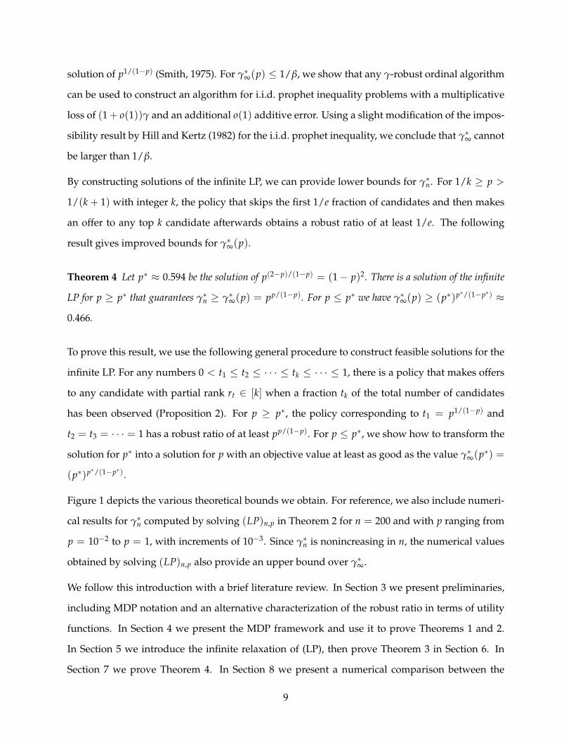
Figure 1 depicts the various theoretical bounds we obtain. For reference, we also include numeri-

cal results for γ∗n computed by solving (LP)n,p in Theorem 2 for n = 200 and with p ranging from

p = 10−2 to p = 1, with increments of 10−3. Since γ∗n is nonincreasing in n, the numerical values

obtained by solving (LP)n,p also provide an upper bound over γ∗∞.

We follow this introduction with a brief literature review. In Section 3 we present preliminaries,

including MDP notation and an alternative characterization of the robust ratio in terms of utility

functions. In Section 4 we present the MDP framework and use it to prove Theorems 1 and 2.

In Section 5 we introduce the infinite relaxation of (LP), then prove Theorem 3 in Section 6. In

Section 7 we prove Theorem 4. In Section 8 we present a numerical comparison between the

9

0.0 0.2 0.4 0.6 0.8 1.0

p

0.3

0.4

0.5

0.6

0.7

0.8

(LP )n,p for n = 200

Upper bound

Lower bound

Figure 1: Bounds for γ∗∞ as a function of p. The solid line represents the theoretical upper boundgiven in Theorem 3. The dashed-dotted line corresponds to the theoretical lower bound given inTheorem 4. In dashed line we present numerical results by solving (LP)n,p for n = 200 candidates.

policies obtained by solving (LP)n,p and other benchmarks policies. We conclude in Section 9,

and an appendix includes proofs and analysis omitted from the main article.

2 Related work

Online advertising and online selection Online advertising has been extensively studied from

the viewpoint of two-sided markets: advertisers and platform. There is extensive work in auction

mechanisms to select ads (e.g. second-price auctions, the VCG mechanism, etc.), and the payment

systems between platforms and advertisers (pay-per-click, pay-for-impression, etc.) (Devanur and

Kakade, 2009; Edelman et al., 2007; Fridgeirsdottir and Najafi-Asadolahi, 2018); see also Choi et al.

(2020) for a review. On the other hand, works relating the platform, advertisers, and web users

have been studied mainly from a learning perspective, to improve ad targeting (Devanur and

Kakade, 2009; Farahat and Bailey, 2012; Hazan, 2019). In this work, we also aim to display an ad

to a potentially interested user. Multiple online selection problems have been proposed to display

ads in online platforms, e.g., packing models (Babaioff et al., 2007; Korula and Pal, 2009), secre-

tary problems and auctions (Babaioff et al., 2008b), prophet models (Alaei et al., 2012) and online

models with ”buyback“ (Babaioff et al., 2008a). In our setting, we add the possibility that a user

ignores the ad; see e.g. Cho and Cheon (2004); Dreze and Hussherr (2003). Failure to click on ads

has been considered in full-information models (Goyal and Udwani, 2020); however, our setting

considers only partial information, where the rank of an incoming customer can only be assessed

10

relative to previously observed customers—a typical occurrence in many online applications. Our

model is also disaggregated and looks at each ad individually. Our goal is to understand the right

time to display an ad/make offers via the SP-UA and the robust ratio for each individual ad.

Online algorithms and arrival models Online algorithms have been extensively studied for ad-

versarial arrivals (Borodin and El-Yaniv, 2005). This worst-case viewpoint gives robust algorithms

against any input sequence, which tend to be conservative. Conversely, some models assume dis-

tributional information about the inputs (Kertz, 1986; Kleywegt and Papastavrou, 1998; Lucier,

2017). The random order model lies in between these two viewpoints, and perhaps the most stud-

ied example is the secretary problem (Dynkin, 1963; Gilbert and Mosteller, 1966; Lindley, 1961).

Random order models have also been applied in Adword problems (Devanur and Hayes, 2009),

online LP’s (Agrawal et al., 2014) and online knapsacks (Babaioff et al., 2007; Kesselheim et al.,

2014), among others.

Secretary problems Martin Gadner popularized the secretary problem in his 1960 Mathematical

Games column; for a historical review, see Ferguson et al. (1989) and also the classical survey

by Freeman (1983). For the classical secretary problem, the optimal strategy that observes the

first n/e candidates and thereafter selects the best candidate was computed by Lindley (1961);

Gilbert and Mosteller (1966). The model has been extensively studied in ordinal/ranked-based

settings (Lindley, 1961; Gusein-Zade, 1966; Vanderbei, 1980; Buchbinder et al., 2014) as well as

cardinal/value-based settings (Bateni et al., 2013; Kleinberg, 2005).

A large body of work has been dedicated to augment the secretary problem. Variations include

cardinality constraints (Buchbinder et al., 2014; Vanderbei, 1980; Kleinberg, 2005), knapsack con-

straints (Babaioff et al., 2007), and matroid constraints (Soto, 2013; Feldman et al., 2014; Lachish,

2014). Model variants also incorporate different arrival processes, such as Markov chains (Hlynka

and Sheahan, 1988) and more general processes (Dutting et al., 2021). Closer to our problem are the

data-driven variations of the model (Correa et al., 2020, 2021; Kaplan et al., 2020), where samples

from the arriving candidates are provided to the decision maker. Our model can be interpreted

as an online version of sampling, where a candidate rejecting the decision maker’s offer is tanta-

11

mount to a sample. This also bears similarity to the exploration-exploitation paradigm often found

in online learning and bandit problems (Cesa-Bianchi and Lugosi, 2006; Hazan, 2019; Freund and

Schapire, 1999).

Uncertain availability in secretary problems The SP-UA is studied by Smith (1975) with the

goal of selecting the top candidate — k = 1 in (1) — who gives an asymptotic probability of

success of p1/(1−p). If the top candidate rejects the offer, this leads to zero value, which is per-

haps excessively pessimistic in scenarios where other competent candidates could accept. Tamaki

(1991) considers maximizing the probability of selecting the top candidate among the candidates

that will accept the offer. Although more realistic, this objective still gives zero value when the

top candidate that accepts is missed because she arrives early in the sequence. In our approach,

we make offers to candidates even if we have already missed the top candidate that accepts the

offer; this is also appealing in utility/value-based settings (see Proposition 1). We also further the

understanding of the model and our objective by presenting closed-form solutions and bounds.

See also Bruss (1987); Presman and Sonin (1973); Cowan and Zabczyk (1979).

Linear programs in secretary problems Early work in secretary problems mostly used MDPs

(Lindley, 1961; Smith, 1975; Tamaki, 1991). Linear programming formulations were introduced by

Buchbinder et al. (2014), and from there multiple formulations have been used to solve variants

of the secretary problem (Chan et al., 2014; Correa et al., 2020; Dutting et al., 2021). We use MDP

to derive the polyhedron that encodes policies for the SP-UA. The connection between linear

programs and MDP has been explored in other online selection and allocation problems, such

as network revenue management (Adelman, 2007), knapsack and prophet problems (Jiang et al.,

2021), more general MDP models (De Farias and Van Roy, 2003; Manne, 1960; Puterman, 2014)

and particularly in constrained MDP’s (Altman, 1999; Haskell and Jain, 2013, 2015). To the best of

our knowledge, these connections have not been explored for secretary problems.

12

3 Preliminaries

To discuss our model, we use standard MDP notation for secretary problems (Dynkin, 1963; Free-

man, 1983; Lindley, 1961). An instance is characterized by the number of candidates n and the

probability p ∈ (0, 1] that an offer is accepted. For t ∈ [n] and s ∈ [t], a state of the system is a

pair (t, s) indicating that the candidate currently being evaluated is the t-th and the corresponding

partial rank is rt = s. To simplify notation, we add the states (n + 1, s), s ∈ [n + 1], and the state

Θ as absorbing states where no decisions can be made. For t < n, transitions from a state (t, s)

to a state (t + 1, σ) are determined by the random permutation π = (R1, . . . , Rn). We denote by

St ∈ {(t, s)}s∈[t] the random variable indicating the state in the t-th stage. A simple calculation

shows

P(St+1 = (t + 1, σ) | St = (t, s)) = P(rt+1 = σ | rt = s) = P(St+1 = (t + 1, σ)) = 1/(t + 1),

for t < n, s ∈ [t] and σ ∈ [t + 1]. In other words, partial ranks at each stage are independent. For

notational convenience, we assume the equality also holds for t = n. Let A = {offer, pass} be the

set of actions. For t ∈ [n], given a state (t, s) and an action At = a ∈ A, the system transitions to a

state St+1 with the following probabilities :

P((t,s),a),(τ,σ) = P(St+1 = (τ, σ) | St = (t, s), At = a) =

1−pt+1 a = offer, τ = t + 1, σ ∈ [τ]

p a = offer, (τ, σ) = Θ

1t+1 a = pass.

The randomness is over the permutation π and the random outcome of the t-th candidate’s de-

cision. We utilize states (n + 1, σ) as end states and the state Θ as the state indicating that an

offer is accepted from the state St. A policy P : {(t, s) : t ∈ [n], s ∈ [t]} → A is a function

that observes a state (t, s) and decides to extend an offer (P(t, s) = offer) or move to the next

candidate (P(t, s) = pass). The policy specifies the actions of a decision maker at any point in

time. The initial state is S1 = (1, 1) and the computation (of a policy) is a sequence of state and

actions (1, 1), a1, (2, s2), a2, (3, s3), . . . where the states transitions according to P((t,s),a),(t+1,σ) and

13

at = P(t, st). Note that the computation always ends in a state (n + 1, σ) for some σ or the state

Θ, either because the policy was able to go through all candidates or because some candidate t

accepted an offer.

We say that a policy reaches stage t or reaches the t-th stage if the computation of a policy contains

a state st = (t, s) for some s ∈ [t]. We also refer to stages as times.

A randomized policy is a function P : {(t, s) : t ∈ [n], s ∈ [t]} → ∆A where ∆A = {(q, 1− q) :

q ∈ [0, 1]} is the probability simplex over A = {offer, pass} and P(st) = (qt, 1− qt) means that P

selects the offer action with probability qt and otherwise selects pass.

We could also define policies that remember previously visited states and at state (t, st) make

decisions based on the history, (1, s1), . . . , (t, st). However, MDP theory guarantees that it suffices

to consider Markovian policies, which make decisions based only on (t, st); see Puterman (2014).

We say that a policy P collects a candidate with rank k if the policy extends an offer to a candidate

that has rank k and the candidate accepts the offer. Thus our objective is to find a policy that solves

γ∗n = maxP

mink∈[n]

P(P collects a candidate with rank ≤ k)1− (1− p)k

= maxP

mink∈[n]

P(P collects a top k candidate | a top k candidate accepts).

The following result is an alternative characterization of γ∗n based on utility functions. We use this

result to relate SP-UA to the i.i.d. prophet inequality problem; the proof appears in Appendix A.1.

Consider a nonzero utility function U : [n] → R+ with U1 ≥ U2 ≥ · · · ≥ Un ≥ 0, and any

rank0based algorithm ALG for the SP-UA, i.e., ALG only makes decisions based on the relative

ranking of the values observed. In the value setting, if ALG collects a candidate with overall rank

i, it obtains value Ui. We denote by U(ALG) the value collected by such an algorithm.

Proposition 1 Let ALG be a γ-robust algorithm for SP-UA. For any U : [n]→ R+ we have E[U(ALG)] ≥

γ E[U(OPT)] where OPT is the maximum value obtained from candidates that accept. Moreover,

γ∗n = maxALG

min{

E [U(ALG)]

E [U(OPT)]: U : [n]→ R+, U 6= 0, U1 ≥ U2 ≥ · · · ≥ Un ≥ 0

}.

14

4 The LP formulation

In this section, we present the proofs of Theorems 1 and 2. Our framework is based on MDP

and can be used to derive similar LPs in the literature, e.g. Buchbinder et al. (2014); Chan et al.

(2014); Correa et al. (2020). As a byproduct, we also show that γ∗n is a nonincreasing sequence

in n (Lemma 1). For ease of explanation, we first present the framework for the classical secre-

tary problem, then we sketch the approach for our model. Technical details are deferred to the

appendix.

4.1 Warm-up: MDP to LP in the classical secretary problem

We next show how to derive an LP for the classical secretary problem (Buchbinder et al., 2014)

using an MDP framework. In this model, the goal is to maximize the probability of choosing the

top candidate, and there is no offer uncertainty.

Theorem 5 (Buchbinder et al. (2014)) The maximum probability of choosing the top-ranked candidate

in the classical secretary problem is given by

max

{n

∑t=1

tn

xt : xt ≤1t

(1−

t−1

∑τ=1

xτ

), ∀t ∈ [n], x ≥ 0

}.

We show this as follows:

1. First, we formulate the secretary problem as a Markov decision process, where we aim to find

the highest ranked candidate. Let v∗(t,s) be the maximum probability of selecting the highest

ranked candidate in t + 1, . . . , n given that the current state is (t, s). We define v∗(n+1,s) = 0

for any s. The value v∗ is called the value function and it can be computed via the optimality

equations (Puterman, 2014)

v∗(t,s) = max

{P(Rt = 1 | rt = s),

1t + 1

t

∑σ=1

v∗(t+1,σ)

}. (2)

The first term in the max operator corresponds to the expected value when the offer action is

chosen in state (t, s). The second corresponds to the expected value in stage t + 1 when we

15

decide to pass in (t, s). Note that P(Rt = 1 | rt = s) = t/n if s = 1 and P(Rt = 1 | rt = s) = 0

otherwise. The optimality equations (2) can be solved via backwards recursion, and v∗(1,1) ≈ 1/e

(for large n). An optimal policy can be obtained from the optimality equations by choosing at

each state an action that attains the maximum, breaking ties arbitrarily.

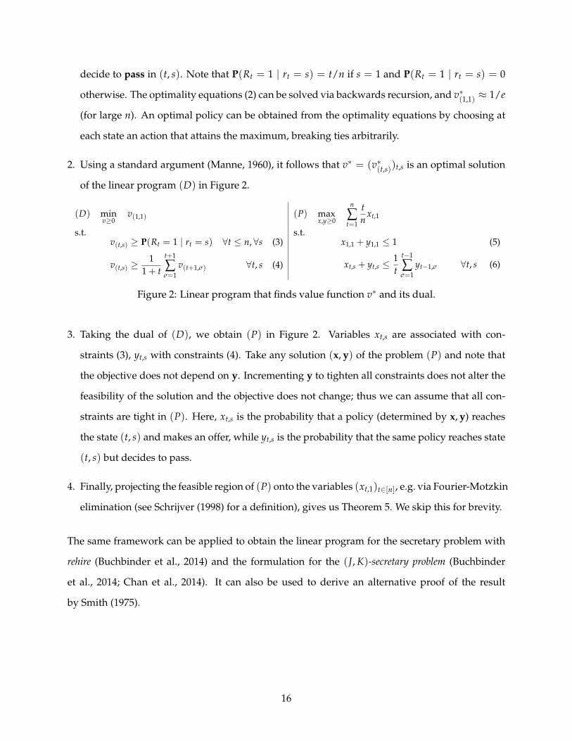
2. Using a standard argument (Manne, 1960), it follows that v∗ = (v∗(t,s))t,s is an optimal solution

of the linear program (D) in Figure 2.

(D) minv≥0

v(1,1) (P) maxx,y≥0

n

∑t=1

tn

xt,1

s.t.v(t,s) ≥ P(Rt = 1 | rt = s) ∀t ≤ n, ∀s (3)

v(t,s) ≥1

1 + t

t+1

∑σ=1

v(t+1,σ) ∀t, s (4)

s.t.x1,1 + y1,1 ≤ 1 (5)

xt,s + yt,s ≤1t

t−1

∑σ=1

yt−1,σ ∀t, s (6)

Figure 2: Linear program that finds value function v∗ and its dual.

3. Taking the dual of (D), we obtain (P) in Figure 2. Variables xt,s are associated with con-

straints (3), yt,s with constraints (4). Take any solution (x, y) of the problem (P) and note that

the objective does not depend on y. Incrementing y to tighten all constraints does not alter the

feasibility of the solution and the objective does not change; thus we can assume that all con-

straints are tight in (P). Here, xt,s is the probability that a policy (determined by x, y) reaches

the state (t, s) and makes an offer, while yt,s is the probability that the same policy reaches state

(t, s) but decides to pass.

4. Finally, projecting the feasible region of (P) onto the variables (xt,1)t∈[n], e.g. via Fourier-Motzkin

elimination (see Schrijver (1998) for a definition), gives us Theorem 5. We skip this for brevity.

The same framework can be applied to obtain the linear program for the secretary problem with

rehire (Buchbinder et al., 2014) and the formulation for the (J, K)-secretary problem (Buchbinder

et al., 2014; Chan et al., 2014). It can also be used to derive an alternative proof of the result

by Smith (1975).

16

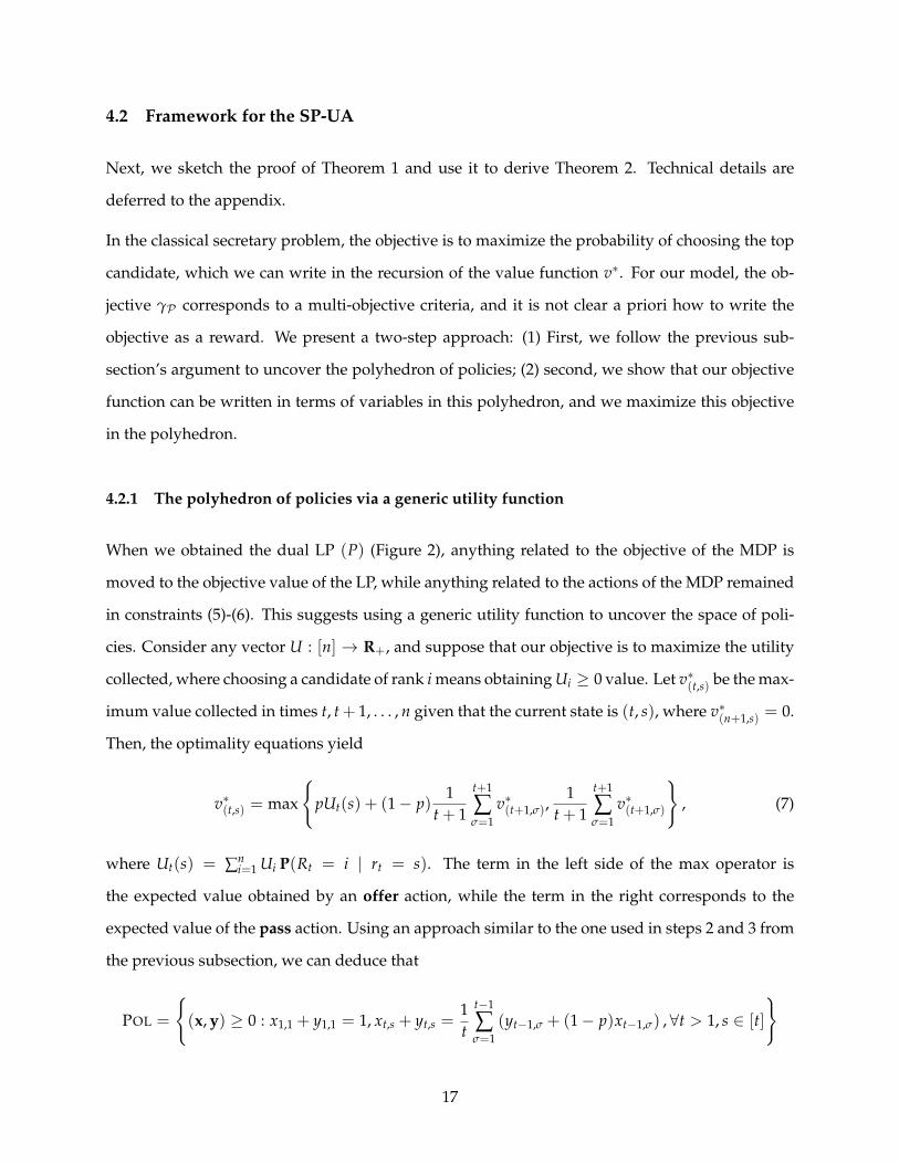
4.2 Framework for the SP-UA

Next, we sketch the proof of Theorem 1 and use it to derive Theorem 2. Technical details are

deferred to the appendix.

In the classical secretary problem, the objective is to maximize the probability of choosing the top

candidate, which we can write in the recursion of the value function v∗. For our model, the ob-

jective γP corresponds to a multi-objective criteria, and it is not clear a priori how to write the

objective as a reward. We present a two-step approach: (1) First, we follow the previous sub-

section’s argument to uncover the polyhedron of policies; (2) second, we show that our objective

function can be written in terms of variables in this polyhedron, and we maximize this objective

in the polyhedron.

4.2.1 The polyhedron of policies via a generic utility function

When we obtained the dual LP (P) (Figure 2), anything related to the objective of the MDP is

moved to the objective value of the LP, while anything related to the actions of the MDP remained

in constraints (5)-(6). This suggests using a generic utility function to uncover the space of poli-

cies. Consider any vector U : [n] → R+, and suppose that our objective is to maximize the utility

collected, where choosing a candidate of rank i means obtaining Ui ≥ 0 value. Let v∗(t,s) be the max-

imum value collected in times t, t + 1, . . . , n given that the current state is (t, s), where v∗(n+1,s) = 0.

Then, the optimality equations yield

v∗(t,s) = max

{pUt(s) + (1− p)

1t + 1

t+1

∑σ=1

v∗(t+1,σ),1

t + 1

t+1

∑σ=1

v∗(t+1,σ)

}, (7)

where Ut(s) = ∑ni=1 Ui P(Rt = i | rt = s). The term in the left side of the max operator is

the expected value obtained by an offer action, while the term in the right corresponds to the

expected value of the pass action. Using an approach similar to the one used in steps 2 and 3 from

the previous subsection, we can deduce that

POL =

{(x, y) ≥ 0 : x1,1 + y1,1 = 1, xt,s + yt,s =

1t

t−1

∑σ=1

(yt−1,σ + (1− p)xt−1,σ) , ∀t > 1, s ∈ [t]

}

17

contains all policies (Theorem 1). A formal proof is presented in the appendix.

4.2.2 The linear program

Next, we consider Theorem 2. Given a policy P , we define xt,s to be the probability of reaching

state (t, s) and making an offer to the candidate, and yt,s to be the probability of reaching (t, s) and

passing. Then (x, y) belongs to POL. Moreover,

P(P collects a top k candidate) = pn

∑t=1

t

∑s=1

xt,s P(Rt ≤ k | rt = s). (8)

Conversely, any point (x, y) ∈ POL defines a policy P : At state (t, s), it extends an offer to the t-th

candidate with probability x1,1 if t = 1, or probability txt,s/(

∑t−1σ=1 yt−1,σ + (1− p)xt−1,σ

)if t > 1.

Also, P satisfies (8). Thus,

γ∗n = maxP

mink∈[n]

P(P collects a top k candidate)1− (1− p)k

= max(x,y)∈POL

mink∈[n]

p ∑nt=1 ∑t

s=1 xt,s P(Rt ≤ k | rt = s)1− (1− p)k

= max{

γ : (x, y) ∈ POL, γ ≤ p ∑nt=1 ∑t

s=1 xt,s P(Rt ≤ k | rt = s)1− (1− p)k , ∀k ∈ [n]

}. (9)

Projecting the feasible region of (9) as in step 4 onto the (x, γ)-variables gives us Theorem 2. The

details appear in Appendix A.2.

Our MDP framework also allows us to show the following monotonicity result.

Lemma 1 For a fixed p ∈ (0, 1], we have γ∗n ≥ γ∗n+1 for any n ≥ 1.

We sketch the proof of this result here and defer the details to Appendix A.3. The dual of the LP (9)

can be reformulated as

minu:[n]→R+

∑i ui≥1

v(1,1)

(DLP) s.t. v(t,s) ≥ max

{Ut(s) +

1− pt + 1

t=1

∑σ=1

v(t+1,σ),1

t + 1

t=1

∑σ=1

v(t+1,σ)

}∀t ∈ [n], s ∈ [t]

v(n+1,s) = 0 ∀s ∈ [n + 1],

18

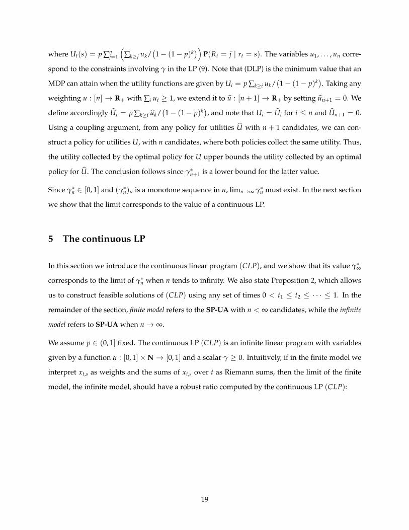
where Ut(s) = p ∑nj=1

(∑k≥j uk/

(1− (1− p)k)) P(Rt = j | rt = s). The variables u1, . . . , un corre-

spond to the constraints involving γ in the LP (9). Note that (DLP) is the minimum value that an

MDP can attain when the utility functions are given by Ui = p ∑k≥i uk/(1− (1− p)k). Taking any

weighting u : [n] → R+ with ∑i ui ≥ 1, we extend it to u : [n + 1] → R+ by setting un+1 = 0. We

define accordingly Ui = p ∑k≥i uk/(1− (1− p)k), and note that Ui = Ui for i ≤ n and Un+1 = 0.

Using a coupling argument, from any policy for utilities U with n + 1 candidates, we can con-

struct a policy for utilities U, with n candidates, where both policies collect the same utility. Thus,

the utility collected by the optimal policy for U upper bounds the utility collected by an optimal

policy for U. The conclusion follows since γ∗n+1 is a lower bound for the latter value.

Since γ∗n ∈ [0, 1] and (γ∗n)n is a monotone sequence in n, limn→∞ γ∗n must exist. In the next section

we show that the limit corresponds to the value of a continuous LP.

5 The continuous LP

In this section we introduce the continuous linear program (CLP), and we show that its value γ∗∞

corresponds to the limit of γ∗n when n tends to infinity. We also state Proposition 2, which allows

us to construct feasible solutions of (CLP) using any set of times 0 < t1 ≤ t2 ≤ · · · ≤ 1. In the

remainder of the section, finite model refers to the SP-UA with n < ∞ candidates, while the infinite

model refers to SP-UA when n→ ∞.

We assume p ∈ (0, 1] fixed. The continuous LP (CLP) is an infinite linear program with variables

given by a function α : [0, 1]×N → [0, 1] and a scalar γ ≥ 0. Intuitively, if in the finite model we

interpret xt,s as weights and the sums of xt,s over t as Riemann sums, then the limit of the finite

model, the infinite model, should have a robust ratio computed by the continuous LP (CLP):

19

(CLP)p

supα:[0,1]×N→[0,1]

γ≥0

γ

s.t.tα(t, s) ≤ 1− p

∫ t

0∑σ≥1

α(τ, σ)dτ ∀t ∈ [0, 1], s ≥ 1

(10)

γ ≤p∫ 1

0 ∑s≥1 α(t, s)∑k`=s (

`−1s−1)t

s(1− t)`−s dt(1− (1− p)k)

∀k ≥ 1

(11)

We denote by γ∗∞ = γ∗∞(p) the objective value of (CLP)p. The following result formalizes the fact

that the value of the continuous LP (CLP)p is in fact the robust ratio of the infinite model. The

proof is similar to other continuous approximations (Chan et al., 2014); a small caveat in the proof

is the restriction of the finite LP to the top (log n)/p candidates, as they carry most of the weight

in the objective function. The proof is deferred to Appendix A.4.

Lemma 2 Let γ∗n be the optimal robust ratio for n candidates and let γ∗∞ be the value of the continuous LP

(CLP)p. Then |γ∗n − γ∗∞| ≤ O((log n)2/

(p√

n))

.

The following proposition gives a recipe to find feasible solutions for (CLP)p. We use it to con-

struct lower bounds in the following sections.

Proposition 2 Consider 0 ≤ t1 ≤ t2 ≤ · · · ≤ 1 and consider the function α : [0, 1]×N→ [0, 1] defined

such that for t ∈ [ti, ti+1)

α(t, s) =

Ti/ti·p+1 s ≤ i

0 s > i,

where Ti = (t1 · · · ti)p. Then α satisfies Constraint (10).

20

Proof We verify that inequality (10) holds. We define t0 = 0 and T0 = 0. For t ∈ [ti, ti+1) we have

1− p∫ t

0∑σ≥1

α(τ, σ)dτ = 1− p

(j−1

∑j=0

∫ tj+1

tj

jTj

τ jp+1 dτ

)− p

∫ t

ti

iTi

τ jp+1 dτ

= 1− pi−1

∑j=0

j · Tj ·1−pj

(t−jp

j+1 − t−jpj

)− pi · Ti ·

1−ip

(t−ip − tip

i

)= 1 +

i−1

∑j=0

Tj

(t−jp

j+1 − t−jpj

)+ Ti

(t−ip − tip

i

)= 1 +

(i−1

∑j=0

Tj+1t−(j+1)pj+1 − Tjt

−jpj

)+ Ti

(t−ip − t−ip

i

)(Since Tj+1t−jp

j+1 = Tj+1t−(j+1)pj+1 )

= 1 + Tit−ipi − T0t−p

0 + Ti

(t−ip − t−ip

i

)= Tit−ip ≥ tα(t, s)

for any s ≥ 1. This concludes the proof. �

We use this result to show lower bounds for γ∗∞. For instance, if 1/k ≥ p > 1/(k + 1) for some

integer k, and we set t1 = 1/e and t2 = t3 = · · · = 1, we can show that γ∗∞(p) is at least 1/e.

Thus, in combination with Lemma 1, we have that γ∗n(p) ≥ 1/e for any n and p > 0; we skip this

analysis for brevity. In Section 7, we use Proposition 2 to show exact solutions of γ∗∞ for large p.

6 Upper bounds for the continuous LP

We now consider upper bounds for (CLP) and prove Theorem 3, which states that γ∗∞(p) ≤

min{

pp/(1−p), 1/β}

, for any p ∈ (0, 1], where 1/β ≈ 0.745 and β is the unique solution of∫ 10 (y(1− log y) + β− 1)−1dy = 1 (Kertz, 1986).

We show that γ∗∞ is bounded by each term in the minimum operator. For the first bound, we have

γ∗n = maxP

mink∈[n]

P(P collects a top k candidate)1− (1− p)k

≤ maxP

P(P collects the top candidate)p

.

21

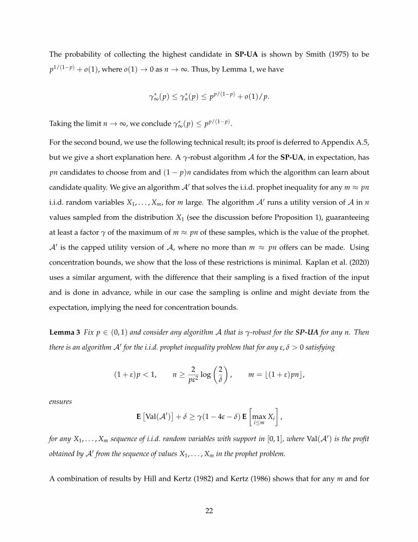
The probability of collecting the highest candidate in SP-UA is shown by Smith (1975) to be

p1/(1−p) + o(1), where o(1)→ 0 as n→ ∞. Thus, by Lemma 1, we have

γ∗∞(p) ≤ γ∗n(p) ≤ pp/(1−p) + o(1)/p.

Taking the limit n→ ∞, we conclude γ∗∞(p) ≤ pp/(1−p).

For the second bound, we use the following technical result; its proof is deferred to Appendix A.5,

but we give a short explanation here. A γ-robust algorithm A for the SP-UA, in expectation, has

pn candidates to choose from and (1− p)n candidates from which the algorithm can learn about

candidate quality. We give an algorithmA′ that solves the i.i.d. prophet inequality for any m ≈ pn

i.i.d. random variables X1, . . . , Xm, for m large. The algorithm A′ runs a utility version of A in n

values sampled from the distribution X1 (see the discussion before Proposition 1), guaranteeing

at least a factor γ of the maximum of m ≈ pn of these samples, which is the value of the prophet.

A′ is the capped utility version of A, where no more than m ≈ pn offers can be made. Using

concentration bounds, we show that the loss of these restrictions is minimal. Kaplan et al. (2020)

uses a similar argument, with the difference that their sampling is a fixed fraction of the input

and is done in advance, while in our case the sampling is online and might deviate from the

expectation, implying the need for concentration bounds.

Lemma 3 Fix p ∈ (0, 1) and consider any algorithm A that is γ-robust for the SP-UA for any n. Then

there is an algorithm A′ for the i.i.d. prophet inequality problem that for any ε, δ > 0 satisfying

(1 + ε)p < 1, n ≥ 2pε2 log

(2δ

), m = b(1 + ε)pnc,

ensures

E[Val(A′)

]+ δ ≥ γ(1− 4ε− δ) E

[maxi≤m

Xi

],

for any X1, . . . , Xm sequence of i.i.d. random variables with support in [0, 1], where Val(A′) is the profit

obtained by A′ from the sequence of values X1, . . . , Xm in the prophet problem.

A combination of results by Hill and Kertz (1982) and Kertz (1986) shows that for any m and for

22

ε′ > 0 small enough, there is an i.i.d. instance X1, . . . , Xm with support in [0, 1] such that

E[

maxi≤m

Xi

]≥ (am − ε′) sup {E[Xτ] : τ ∈ Tm} ,

where Tm is the class of stopping times for X1, . . . , Xm, and am → β. Thus, using Lemma 3, for any

γ such that a γ-robust algorithm A exists for the SP-UA, we must have

γ(1− 4ε− δ) ≤ 1am − ε′

+δ

E [maxi≤m Xi]

for m = b(1 + ε)pnc; here we set δ = 2e−pn2/2. A slight reformulation of Hill and Kertz’s re-

sult allows us to set ε′ = 1/m3 and E[maxi≤m Xi] ≥ 1/m3 (see the discussion at the end of Ap-

pendix A.5). Thus, as n→ ∞ we have m→ ∞ and so δ/ E[maxi≤m Xi]→ 0. In the limit we obtain

γ(1− 4ε) ≤ 1/β for any ε > 0 such that (1 + ε)p < 1. From here, the upper bound γ ≤ 1/β

follows.

An algorithm that solves (LP)n,p and implements the policy given by the solution is γ∗∞-robust

(Theorem 2 and the fact that γ∗n ≥ γ∗∞) for any n. Thus, by the previous analysis and Lemma 1, we

obtain γ∗∞ ≤ 1/β.

7 Lower bounds for the continuous LP

In this section we consider lower bounds for (CLP) and prove Theorem 4. We first give optimal

solutions for large values of p. For p ≥ p∗ ≈ 0.594, the optimal value of (CLP)p is γ∗∞(p) =

pp/(1−p). We then show that for p ≤ p∗, γ∗∞(p) ≥ (p∗)p∗/(1−p∗) ≈ 0.466.

7.1 Exact solution for large p

We now show that for p ≥ p∗, γ∗∞(p) = pp/(1−p), where p∗ ≈ 0.594 is the solution of (1− p)2 =

p(2−p)/(1−p). Thanks to the upper bound γ∗∞(p) ≤ pp/(1−p) for any p ∈ (0, 1], it is enough to exhibit

feasible solutions (α, γ) of the continuous LP (CLP)p with γ ≥ pp/(1−p).

Let t1 = p1/(1−p), t2 = t3 = · · · = 1, and consider the function α defined by t1, t2, . . . in Proposi-

23

tion 2. That is, for t ∈ [0, p1/(1−p)), α(t, s) = 0 for any s ≥ 1 and for t ∈ [p1/(1−p), 1] we have

α(t, s) =

pp/(1−p)/t1+p s = 1

0 s > 1.

Let γ.= infk≥1 p

(1− (1− p)k)−1 ∫ 1

p1/(1−p)pp/(1−p)

t1+p ∑k`=1 t(1− t)`−1dt. Then (α, γ) is feasible for the

continuous LP (CLP)p, and we aim to show that γ ≥ pp/(1−p) when p ≥ p∗. The result follows by

the following lemma.

Lemma 4 For any p ≥ p∗ and any ` ≥ 0,∫ 1

p1/(1−p) (1− t)`t−p dt ≥ (1− p)`.

We defer the proof of this lemma to Appendix A.6. Now, we have

γ = infk≥1

p1− (1− p)k

∫ 1

p1/1−p

pp/(1−p)

t1+p

k

∑`=1

t(1− t)`−1dt

= pp/(1−p) infk≥1

∑k`=1∫ 1

p1/(1−p) t−p(1− t)`−1 dt

∑k`=1(1− p)`−1

≥ pp/(1−p) infk≥1

inf`∈[k]

∫ 1

0

1tp

(1− t)`−1

(1− p)`−1 dt ≥ pp/(1−p),

where we use the known inequality ∑m`=1 a`/∑m

`=1 b` ≥ min`∈[m] a`/b` for a`, b` > 0, for any `, and

the lemma. This shows that γ∗∞ ≥ pp/(1−p) for p ≥ p∗.

Remark 1 Our analysis is tight. For k = 2, constraint

p1− (1− p)2

∫ 1

p1/(1−p)

pp/(1−p)

t1+p

k

∑`=1

t(1− t)`−1 dt ≥ pp/(1−p)

holds if and only if p ≥ p∗.

7.2 Lower bound for small p

We now argue that for p ≤ p∗, γ∗∞(p) ≥ (p∗)p∗/(1−p∗). Let ε ∈ [0, 1) satisfy p = (1− ε)p∗. For

the argument, we take the solution α∗ for (CLP)p∗ that we obtained in the last subsection and we

construct a feasible solution for (CLP)p with objective value at least (p∗)p∗/(1−p∗). For simplicity,

24

we denote τ∗ = (p∗)1/(1−p∗).

From the previous subsection, we know that the optimal solution α∗ of (CLP)p∗ has the following

form. For t ∈ [0, τ∗), α∗(t, s) = 0 for any s, while for t ∈ [τ∗, 1] we have

α∗(t, s) =

(p∗)p∗/(1−p∗)/tp∗+1 s = 1

0 s > 1.

For (CLP)p, we construct a solution α as follows. Let α(t, s) = εs−1α∗(t, 1) for any t ∈ [0, 1] and

s ≥ 1; for example, α(t, 1) = α∗(t, 1). If we interpret α∗ as a policy, it only makes offers to the

highest candidate observed. By contrast, in (CLP)p the policy implied by α makes offers to more

candidates (after time τ∗), with a probability geometrically decreasing according to the relative

ranking of the candidate.

Claim 7.1 The solution α satisfies constraints (10),

tα(t, s) ≤ 1− p∫ t

0∑σ≥1

α(τ, σ)dτ,

for any t ∈ [0, 1], s ≥ 1.

Proof Indeed,

1− p∫ t

0∑σ≥1

α(τ, σ)dτ = 1− p∗(1− ε)∫ t

0∑σ≥1

εσ−1α∗(τ, 1)dτ

= 1− p∗∫ t

0α∗(τ, 1)dτ (Since ∑σ≥1 εσ−1 = 1/(1− ε))

= 1− p∗∫ t

0∑σ≥1

α∗(τ, σ)dτ (Since α∗(τ, σ) = 0 for σ > 1)

≥ tα∗(t, 1). (By feasibility of α∗)

Since α(t, s) = εs−1α∗(t, 1) ≤ α∗(t, 1), we conclude that α satisfies (10) for any t and s. �

We now define γ = infk≥1 p(1− (1− p)k)−1 ∫ 1

0 ∑s≥1 α(t, s)∑k`=s (

`−1s−1)t

s(1 − t)`−sdt. Using the

claim, we know that (α, γ) is feasible for (CLP)p, and need to verify that γ ≥ (p∗)p∗/(1−p∗). Similar

25

to the analysis in the previous section, the result follows by the following claim.

Claim 7.2 For any ` ≥ 0,∫ 1

τ∗ (1− (1− ε)t)`t−p∗ dt ≥ (1− p)`.

Before proving the claim, we establish the bound:

γ = infk≥1

1

∑k`=1(1− p)`−1

∫ 1

0

k

∑s=1

εs−1α∗(s, 1)k

∑`=s

(`− 1s− 1

)ts(1− t)`−s dt (Using definition of α)

= (p∗)p∗/(1−p∗) infk≥1

1

∑k`=1(1− p)`−1

∫ 1

τ∗

1tp∗+1

k

∑`=1

`

∑s=1

εs−1(`− 1s− 1

)ts(1− t)`−s dt

(Using the definition of α∗ and changing order of summmation)

= (p∗)p∗/(1−p∗) infk≥1

1

∑k`=1(1− p)`−1

∫ 1

τ∗

1tp∗+1

k

∑`=1

(1− (1− ε)t)`−1 dt

(Using the binomial expansion)

= (p∗)p∗/(1−p∗) infk≥1

∑k`=1∫ 1

τ∗ t−p∗−1(1− (1− ε)t)`−1 dt

∑k`=1(1− p)`−1

≥ (p∗)p∗/(1−p∗)

We again used the inequality ∑m`=1 a`/∑m

`=1 b` ≥ min`∈[m] a`/b` for a`, b` > 0, for any `, and the

claim.

Proof of Claim 7.2 We have 1− (1− ε)t = (1− ε)(1− t) + ε. Therefore,

∫ 1

τ∗

1tp∗ (1− (1− ε)t)`dt =

∫ 1

τ∗

1tp∗

`

∑j=0

(`

j

)(1− ε)`−j(1− t)`−jε`−jdt (Binomial expansion)

=`

∑j=0

(`

j

)(1− ε)`−jεj

∫ 1

τ∗

1tp∗ (1− t)`−j dt

≥`

∑j=0

(`

j

)(1− ε)`−jεj(1− p∗)`−j dt (Using Lemma 4 for p∗)

= (ε + (1− ε)(1− p∗))` (Using binomial expansion)

= (1− (1− ε)p∗)` = (1− p)`,

where we used p = (1− ε)p∗. From this inequality the claim follows. �

26

8 Computational experiments

In this section we aim to empirically test our policy; to do so, we focus on utility models. Recall

from Proposition 1 that a γ-robust policy ensures at least γ fraction of the optimal offline utility,

for any utility functions that is related to the ranking, i.e., Uj < Ui if and only if i ≺ j. This is ad-

vantageous for practical scenarios, where a candidate’s “value” may be unknown to the decision

maker.

We evaluate the performance of two groups of solutions. The first group includes policies that are

computed without the knowledge of any utility function:

• Robust policy (Rob-Pol(n, p)), corresponds to the optimal policy obtained by solving (LP)n,p.

• Tamaki’s policy (Tama-Pol(n, p)), that maximizes the probability of selecting successfully the

best candidate willing to accept an offer. To be precise, Tamaki (1991) studies two models of

availability: MODEL 1, where the availability of the candidate is known after an offer has been

made; and MODEL 2, where the availability of the candidate is known upon the candidate’s

arrival. MODEL 2 has higher values and it is computationally less expensive to compute; we

use this policy. Note that in SP-UA, the expected value obtained by learning the availability

of the candidate after making an offer is the same value obtained in the model that learns the

availability right upon arrival. Therefore, MODEL 2 is a better model to compare our solutions

than MODEL 1.

In the other group, we have policies that are computed with knowledge of the utility function.

• The expected optimal offline value (E[U(OPT(U, n, p))]), which knows the outcome of the of-

fers and the utility function. It can be computed via ∑ni=1 Ui p(1− p)i−1. For simplicity, we write

OPT when the parameters are clear from the context.

• The optimal rank-based policy if the utility function is known in advance, (Util-Pol(U, n, p)),

computed by solving the optimality equation

v(t,s) = max

{Ut(s) +

1− pt + 1

t+1

∑σ=1

v(t+1,σ),1

t + 1

t+1

∑σ=1

v(t+1,σ),

},

27

with boundary condition v(n+1,σ) = 0 for any σ. We write Util-Pol(n, p) when U is clear from

the context. We use a rank-based policy as opposed to a value-based policy for computational

efficiency.

Note that E[U(Rob-Pol)], E[U(Tama-Pol)] ≤ E[U(Util-Pol)] ≤ E[U(OPT)] and by Proposition 1,

E[U(Rob-Pol)] ≥ γ∗n E[U(A)] for any A of the aforementioned policies.

We consider the following decreasing utility functions:

• Top k candidates are valuable (top-k). For k ∈ [n], we consider utility functions of the form

Ui = 1 + εi for i ∈ [k] and Ui = εi for i > k with ε = 1/n. Intuitively, we aim to capture

the notion of an elite set of candidates, where candidates outside the top k are not nearly as

appealing to the decision maker. For instance, renowned brands like to target certain members

of a population for their ads. We test k = 1, 2, 3, 4.

• Power law population. Ui = i−1/(1+δ) for i ≥ 1 and small δ > 0. Empirical studies have

shown that the distribution of individual performances in many areas follows a power law or

Pareto distribution (Clauset et al., 2009). If we select a random person from [n], the probability

that this individual has a performance score of at least t is proportional to t−(1+δ). We test

δ ∈ {10−2, 10−1, 2 · 10−1}.

We run experiments for n = 200 candidates and range the probability of acceptance p from p =

10−2 to p = 9 · 10−1.

8.1 Results for top-k utility function

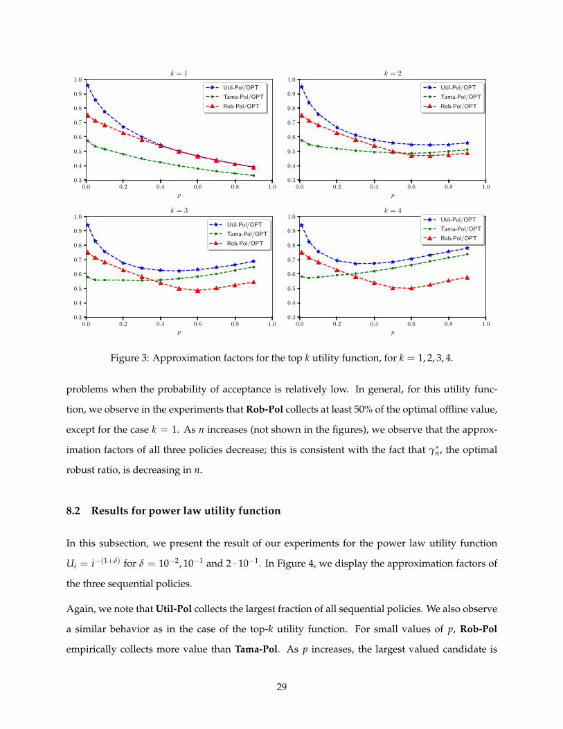
In this subsection, we present the results for utility function that has largest values in the top k

candidates, where k = 1, 2, 3, 4. In Figure 3, we plot the ratio between the value collected by A

and E[U(OPT)], for A being Util-Pol, Rob-Pol and Tama-Pol.

Naturally, of all sequential policies, Util-Pol attains the largest approximation factor of E[U(OPT)].

We observe empirically that Rob-Pol collects larger values than Tama-Pol for smaller values of k.

Interestingly, we observe in the four experiments that the approximation factor for Rob-Pol is al-

ways better than Tama-Pol for small values of p. In other words, robustness helps online selection

28

0.0 0.2 0.4 0.6 0.8 1.0

p

0.3

0.4

0.5

0.6

0.7

0.8

0.9

1.0k = 1

Util-Pol/OPT

Tama-Pol/OPT

Rob-Pol/OPT

0.0 0.2 0.4 0.6 0.8 1.0

p

0.3

0.4

0.5

0.6

0.7

0.8

0.9

1.0k = 2

Util-Pol/OPT

Tama-Pol/OPT

Rob-Pol/OPT

0.0 0.2 0.4 0.6 0.8 1.0

p

0.3

0.4

0.5

0.6

0.7

0.8

0.9

1.0k = 3

Util-Pol/OPT

Tama-Pol/OPT

Rob-Pol/OPT

0.0 0.2 0.4 0.6 0.8 1.0

p

0.3

0.4

0.5

0.6

0.7

0.8

0.9

1.0k = 4

Util-Pol/OPT

Tama-Pol/OPT

Rob-Pol/OPT

Figure 3: Approximation factors for the top k utility function, for k = 1, 2, 3, 4.

problems when the probability of acceptance is relatively low. In general, for this utility func-

tion, we observe in the experiments that Rob-Pol collects at least 50% of the optimal offline value,

except for the case k = 1. As n increases (not shown in the figures), we observe that the approx-

imation factors of all three policies decrease; this is consistent with the fact that γ∗n, the optimal

robust ratio, is decreasing in n.

8.2 Results for power law utility function

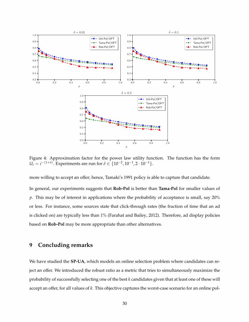
In this subsection, we present the result of our experiments for the power law utility function

Ui = i−(1+δ) for δ = 10−2, 10−1 and 2 · 10−1. In Figure 4, we display the approximation factors of

the three sequential policies.

Again, we note that Util-Pol collects the largest fraction of all sequential policies. We also observe

a similar behavior as in the case of the top-k utility function. For small values of p, Rob-Pol

empirically collects more value than Tama-Pol. As p increases, the largest valued candidate is

29

0.0 0.2 0.4 0.6 0.8 1.0

p

0.3

0.4

0.5

0.6

0.7

0.8

0.9

1.0δ = 0.01

Util-Pol/OPT

Tama-Pol/OPT

Rob-Pol/OPT

0.0 0.2 0.4 0.6 0.8 1.0

p

0.3

0.4

0.5

0.6

0.7

0.8

0.9

1.0δ = 0.1

Util-Pol/OPT

Tama-Pol/OPT

Rob-Pol/OPT

0.0 0.2 0.4 0.6 0.8 1.0

p

0.3

0.4

0.5

0.6

0.7

0.8

0.9

1.0δ = 0.2

Util-Pol/OPT

Tama-Pol/OPT

Rob-Pol/OPT

Figure 4: Approximation factor for the power law utility function. The function has the formUi = i−(1+δ). Experiments are run for δ ∈ {10−2, 10−1, 2 · 10−1}.

more willing to accept an offer; hence, Tamaki’s 1991 policy is able to capture that candidate.

In general, our experiments suggests that Rob-Pol is better than Tama-Pol for smaller values of

p. This may be of interest in applications where the probability of acceptance is small, say 20%

or less. For instance, some sources state that click-through rates (the fraction of time that an ad

is clicked on) are typically less than 1% (Farahat and Bailey, 2012). Therefore, ad display policies

based on Rob-Pol may be more appropriate than other alternatives.

9 Concluding remarks

We have studied the SP-UA, which models an online selection problem where candidates can re-

ject an offer. We introduced the robust ratio as a metric that tries to simultaneously maximize the

probability of successfully selecting one of the best k candidates given that at least one of these will

accept an offer, for all values of k. This objective captures the worst-case scenario for an online pol-

30

icy against an offline adversary that knows in advance which candidates will accept an offer. We

also demonstrated a connection between this robust ratio and online selection with utility func-

tions. We presented a framework based on MDP theory to derive a linear program that computes

the optimal robust ratio and its optimal policy. This framework can be generalized and used in

other secretary problems (Section 4.1), for instance, by augmenting the state space. Furthermore,

using the MDP framework, we were able to show that the robust ratio γ∗n is a decreasing func-

tion in n. This enabled us to make connections between early works in secretary problems and

recent advances. To study our LP, we allow the number of candidates to go to infinity and obtain

a continuous LP. We provide bounds for this continuous LP, and optimal solutions for large p.

We empirically observe that the robust ratio γ∗n(p) is convex and decreasing as a function of p, and

thus we expect the same behavior from γ∞(p), though this remains to be proved (see Figure 1).

Based on numerical values obtained by solving (LP)n,p, we conjecture that limp→0 γ∗∞(p) = 1/β ≈

0.745. This limit is also observed in a similar model (Correa et al., 2020), where a fraction of the

input is given in advance to the decision maker as a sample. In our model, if we interpret the

rejection from a candidate as a sample, then in the limit both models might behave similarly.

Numerical comparisons between our policies and benchmarks suggest that our proposed policies

perform especially well in situations where the probability of acceptance is small, say less than

20%, as in the case of online advertisement.

A natural extension is the value-based model, where candidates reveal numerical values instead

of partial rankings. Our algorithms are rank-based and guarantee an expected value at least a frac-

tion γ∗n(p) of the optimal offline expected value (Proposition 1). Nonetheless, algorithms based on

numerical values may attain higher expected values than the ones guaranteed by our algorithm.

In fact, a threshold algorithm based on sampling may perhaps be enough to guarantee better

values, although this this requires an instance-dependent approach. The policies we consider

are instance-agnostic, can be computed once and used for any input sequence of values. In this

value-based model, we would like to consider other arrivals processes. A popular arrival model

is the adversarial arrival, where an adversary constructs values and the arrival order in response

to the DM’s algorithm. Unfortunately, a construction similar to the one in Marchetti-Spaccamela

and Vercellis (1995) for the online knapsack problem shows that it is impossible to attain a finite

31

competitive ratio in an adversarial regime.

Customers belonging to different demographic groups may have different willingness to click on

ads (Cheng and Cantu-Paz, 2010). In this work, we considered a uniform probability of accep-

tance, and our techniques do not apply directly in the case of different probabilities. In ad display,

one way to cope with different probabilities depending on customers’ demographic group is the

following. Upon observing a customer, a random variable (independent of the ranking of the can-

didate) signals the group of the customer. The probability of acceptance of a candidate depends

on the candidate’s group. Assuming independence between the rankings and the demographic

group allows us to learn nothing about the global quality of the candidates beyond what we can

learn from the partial rank. Using the framework presented in this work, with an augmented state

space (time, partial rank, group type), we can write an LP that solves this problem exactly. Never-

theless, understanding the robust ratio in this new setting and providing a closed-form policy are

still open questions.

Another interesting extension is the case of multiple selections. In practice, platforms can display

the same ad to more than one user, and some job posts require more than one person for a position.

In this setting, the robust ratio is less informative. If k is the number of possible selections, one

possible objective is to maximize the number of top k candidates selected. We can apply the

framework from this work to obtain an optimal LP. Although there is an optimal solution, no

simple closed-form strategies have been found even for p = 1; see e.g. Buchbinder et al. (2014)).

References

Daniel Adelman. Dynamic bid prices in revenue management. Operations Research, 55(4):647–661, 2007.

Shipra Agrawal, Zizhuo Wang, and Yinyu Ye. A dynamic near-optimal algorithm for online linear pro-gramming. Operations Research, 62(4):876–890, 2014.

Saeed Alaei, MohammadTaghi Hajiaghayi, and Vahid Liaghat. Online prophet-inequality matching withapplications to ad allocation. In Proceedings of the 13th ACM Conference on Electronic Commerce, pages18–35, 2012.

Eitan Altman. Constrained Markov decision processes, volume 7. CRC Press, 1999.

Moshe Babaioff, Nicole Immorlica, David Kempe, and Robert Kleinberg. A knapsack secretary problemwith applications. In Approximation, randomization, and combinatorial optimization. Algorithms and tech-niques, pages 16–28. Springer, 2007.

Moshe Babaioff, Jason Hartline, and Robert Kleinberg. Selling banner ads: Online algorithms with buyback.In Fourth Workshop on Ad Auctions, 2008a.

32

Moshe Babaioff, Nicole Immorlica, David Kempe, and Robert Kleinberg. Online auctions and generalizedsecretary problems. ACM SIGecom Exchanges, 7(2):1–11, 2008b.

MohammadHossein Bateni, Mohammadtaghi Hajiaghayi, and Morteza Zadimoghaddam. Submodularsecretary problem and extensions. ACM Transactions on Algorithms (TALG), 9(4):1–23, 2013.

Allan Borodin and Ran El-Yaniv. Online computation and competitive analysis. cambridge university press,2005.

Stephane Boucheron, Gabor Lugosi, and Pascal Massart. Concentration inequalities: A nonasymptotic theory ofindependence. Oxford university press, 2013.

F Thomas Bruss. On an optimal selection problem of cowan and zabczyk. Journal of Applied Probability,pages 918–928, 1987.

Niv Buchbinder, Kamal Jain, and Mohit Singh. Secretary problems via linear programming. Mathematics ofOperations Research, 39(1):190–206, 2014.

Gregory Campbell and Stephen M Samuels. Choosing the best of the current crop. Advances in AppliedProbability, 13(3):510–532, 1981.

Nicolo Cesa-Bianchi and Gabor Lugosi. Prediction, learning, and games. Cambridge university press, 2006.

TH Hubert Chan, Fei Chen, and Shaofeng H-C Jiang. Revealing optimal thresholds for generalized secre-tary problem via continuous lp: impacts on online k-item auction and bipartite k-matching with randomarrival order. In Proceedings of the Twenty-Sixth Annual ACM-SIAM Symposium on Discrete Algorithms,pages 1169–1188. SIAM, 2014.

Haibin Cheng and Erick Cantu-Paz. Personalized click prediction in sponsored search. In Proceedings of thethird ACM international conference on Web search and data mining, pages 351–360, 2010.

Chang-Hoan Cho and Hongsik John Cheon. Why do people avoid advertising on the internet? Journal ofadvertising, 33(4):89–97, 2004.

Hana Choi, Carl F Mela, Santiago R Balseiro, and Adam Leary. Online display advertising markets: Aliterature review and future directions. Information Systems Research, 31(2):556–575, 2020.

Aaron Clauset, Cosma Rohilla Shalizi, and Mark EJ Newman. Power-law distributions in empirical data.SIAM review, 51(4):661–703, 2009.

Jose Correa, Andres Cristi, Boris Epstein, and Jose Soto. Sample-driven optimal stopping: From the secre-tary problem to the iid prophet inequality. arXiv preprint arXiv:2011.06516, 2020.

Jose Correa, Andres Cristi, Laurent Feuilloley, Tim Oosterwijk, and Alexandros Tsigonias-Dimitriadis. Thesecretary problem with independent sampling. In Proceedings of the 2021 ACM-SIAM Symposium on Dis-crete Algorithms (SODA), pages 2047–2058. SIAM, 2021.

Richard Cowan and Jerzy Zabczyk. An optimal selection problem associated with the poisson process.Theory of Probability & Its Applications, 23(3):584–592, 1979.

Daniela Pucci De Farias and Benjamin Van Roy. The linear programming approach to approximate dynamicprogramming. Operations research, 51(6):850–865, 2003.

Nikhil R Devanur and Thomas P Hayes. The adwords problem: online keyword matching with budgetedbidders under random permutations. In Proceedings of the 10th ACM conference on Electronic commerce,pages 71–78, 2009.

Nikhil R Devanur and Sham M Kakade. The price of truthfulness for pay-per-click auctions. In Proceedingsof the 10th ACM conference on Electronic commerce, pages 99–106, 2009.

Xavier Dreze and Francois-Xavier Hussherr. Internet advertising: Is anybody watching? Journal of interac-tive marketing, 17(4):8–23, 2003.

Paul Dutting, Silvio Lattanzi, Renato Paes Leme, and Sergei Vassilvitskii. Secretaries with advice. In Pro-ceedings of the 22nd ACM Conference on Economics and Computation, pages 409–429, 2021.

Evgenii Borisovich Dynkin. The optimum choice of the instant for stopping a markov process. Soviet

33

Mathematics, 4:627–629, 1963.

Benjamin Edelman, Michael Ostrovsky, and Michael Schwarz. Internet advertising and the generalizedsecond-price auction: Selling billions of dollars worth of keywords. American economic review, 97(1):242–259, 2007.

Ayman Farahat and Michael C Bailey. How effective is targeted advertising? In Proceedings of the 21stinternational conference on World Wide Web, pages 111–120, 2012.

Moran Feldman, Ola Svensson, and Rico Zenklusen. A simple o (log log (rank))-competitive algorithm forthe matroid secretary problem. In Proceedings of the twenty-sixth annual ACM-SIAM symposium on Discretealgorithms, pages 1189–1201. SIAM, 2014.

Thomas S Ferguson et al. Who solved the secretary problem? Statistical science, 4(3):282–289, 1989.

PR Freeman. The secretary problem and its extensions: A review. International Statistical Review/RevueInternationale de Statistique, pages 189–206, 1983.

Yoav Freund and Robert E Schapire. Adaptive game playing using multiplicative weights. Games andEconomic Behavior, 29(1-2):79–103, 1999.

Kristin Fridgeirsdottir and Sami Najafi-Asadolahi. Cost-per-impression pricing for display advertising.Operations Research, 66(3):653–672, 2018.

John P Gilbert and Frederick Mosteller. Recognizing the maximum of a sequence. Journal of the AmericanStatistical Association, pages 35–73, 1966.

Vineet Goyal and Rajan Udwani. Online matching with stochastic rewards: Optimal competitive ratio viapath based formulation. In Proceedings of the 21st ACM Conference on Economics and Computation, pages791–791, 2020.

SM Gusein-Zade. The problem of choice and the sptimal stopping rule for a sequence of independent trials.Theory of Probability & Its Applications, 11(3):472–476, 1966.

William B Haskell and Rahul Jain. Stochastic dominance-constrained markov decision processes. SIAMJournal on Control and Optimization, 51(1):273–303, 2013.

William B Haskell and Rahul Jain. A convex analytic approach to risk-aware markov decision processes.SIAM Journal on Control and Optimization, 53(3):1569–1598, 2015.

Elad Hazan. Introduction to online convex optimization. arXiv preprint arXiv:1909.05207, 2019.

Theodore P Hill and Robert P Kertz. Comparisons of stop rule and supremum expectations of iid randomvariables. The Annals of Probability, pages 336–345, 1982.

M Hlynka and JN Sheahan. The secretary problem for a random walk. Stochastic Processes and their applica-tions, 28(2):317–325, 1988.

Jiashuo Jiang, Will Ma, and Jiawei Zhang. Tight guarantees for multi-unit prophet inequalities and onlinestochastic knapsack. arXiv preprint arXiv:2107.02058, 2021.

Haim Kaplan, David Naori, and Danny Raz. Competitive analysis with a sample and the secretary problem.In Proceedings of the Fourteenth Annual ACM-SIAM Symposium on Discrete Algorithms, pages 2082–2095.SIAM, 2020.

Robert P Kertz. Stop rule and supremum expectations of iid random variables: a complete comparison byconjugate duality. Journal of multivariate analysis, 19(1):88–112, 1986.

Thomas Kesselheim, Andreas Tonnis, Klaus Radke, and Berthold Vocking. Primal beats dual on onlinepacking lps in the random-order model. In Proceedings of the forty-sixth annual ACM symposium on Theoryof computing, pages 303–312, 2014.

Robert Kleinberg. A multiple-choice secretary algorithm with applications to online auctions. In Proceedingsof the sixteenth annual ACM-SIAM symposium on Discrete algorithms, pages 630–631. Citeseer, 2005.

Anton J Kleywegt and Jason D Papastavrou. The dynamic and stochastic knapsack problem. Operationsresearch, 46(1):17–35, 1998.

34

Nitish Korula and Martin Pal. Algorithms for secretary problems on graphs and hypergraphs. In Interna-tional Colloquium on Automata, Languages, and Programming, pages 508–520. Springer, 2009.

Oded Lachish. O (log log rank) competitive ratio for the matroid secretary problem. In 2014 IEEE 55thAnnual Symposium on Foundations of Computer Science, pages 326–335. IEEE, 2014.

Denis V Lindley. Dynamic programming and decision theory. Journal of the Royal Statistical Society: Series C(Applied Statistics), 10(1):39–51, 1961.

Brendan Lucier. An economic view of prophet inequalities. ACM SIGecom Exchanges, 16(1):24–47, 2017.

A.S. Manne. Linear Programming and Sequential Decisions. Management Science, 6:259–267, 1960.

Alberto Marchetti-Spaccamela and Carlo Vercellis. Stochastic on-line knapsack problems. MathematicalProgramming, 68(1):73–104, 1995.

Aranyak Mehta, Bo Waggoner, and Morteza Zadimoghaddam. Online stochastic matching with unequalprobabilities. In Proceedings of the twenty-sixth annual ACM-SIAM symposium on Discrete algorithms, pages1388–1404. SIAM, 2014.

Ernst L Presman and Isaac Mikhailovich Sonin. The best choice problem for a random number of objects.Theory of Probability & Its Applications, 17(4):657–668, 1973.

Enric Pujol, Oliver Hohlfeld, and Anja Feldmann. Annoyed users: Ads and ad-block usage in the wild. InProceedings of the 2015 Internet Measurement Conference, pages 93–106, 2015.

Martin L Puterman. Markov decision processes: discrete stochastic dynamic programming. John Wiley & Sons,2014.

Manish Raghavan, Solon Barocas, Jon M Kleinberg, and Karen Levy. Mitigating bias in algorithmic em-ployment screening: Evaluating claims and practices. 2019.

Jad Salem and Swati Gupta. Closing the gap: Group-aware parallelization for the secretary problem withbiased evaluations. Available at SSRN 3444283, 2019.

Alexander Schrijver. Theory of linear and integer programming. John Wiley & Sons, 1998.

MH Smith. A secretary problem with uncertain employment. Journal of applied probability, pages 620–624,1975.

Jose A Soto. Matroid secretary problem in the random-assignment model. SIAM Journal on Computing, 42(1):178–211, 2013.

Mitsushi Tamaki. A secretary problem with uncertain employment and best choice of available candidates.Operations Research, 39(2):274–284, 1991.

Robert J Vanderbei. The optimal choice of a subset of a population. Mathematics of Operations Research, 5(4):481–486, 1980.

Robert J Vanderbei. The postdoc variant of the secretary problem. Technical report, Technical report, Prince-ton University, 2012.

A Appendix

A.1 Missing proofs from Section 3

Proof of Proposition 1 Let ALG be a γ-robust algorithm. Fix any algorithm ALG and any U1 ≥ · · · ≥ Un ≥

0. Let ε > 0 and let Ui = Ui + εi. Thus Ui > Ui+1 and so rank and utility are in one-to-one correspondence.

35

Then

E[U(ALG)]

E[U(OPT)]≥ min

x∈{U1,...,Un}

P(U(ALG) ≥ x)P(U(OPT) ≥ x)

= mink≤n

P(ALG collects a top k candidate)P(A top k candidate accepts)

≥ γ

where we used the fact that ALG is γ-robust. Notice that E[U(OPT)] ≤ E[U(OPT)], and also E[U(ALG)] ≤

E[U(ALG)] + ε. Thus doing ε→ 0 we obtain

E[U(ALG)]

E[U(OPT)]≥ γ (12)

for any nonzero vector U with U1 ≥ U2 ≥ · · · ≥ Un ≥ 0. This finishes the first part. For the second part, let

γn = minALG

max{

E[U(ALG)]

E[U(OPT)]: U : [n]→ R+, U1 ≥ · · · ≥ Un

}.

Note that the RHS of Inequality (12) is independent of U, thus minimizing in U in the LHS and then

maximizing in ALG on both sides we obtain γn ≥ γ∗n.

To show the reverse inequality, fix k ∈ [n] and let U : [n] → R+ given by Ui = 1 for i ≤ k and Ui = 0 for

i > k. Then,

P(ALG collects a top k candidate)P(A top k candidate accepts)

=E[U(ALG)]

E[U(OPT)]≥ min

U:[n]→R+U1≥···≥Un

E[U(ALG)]

E[U(OPT)].

This bound holds for any k, thus minimizing over k and then maximizing over ALG on both sides, we

obtain γ∗n ≥ γn, which finishes the second part. �

A.2 Missing proofs from Section 4

Here we present a detailed derivation of Theorem 1 and Theorem 2 by revisiting Section 4.

As stated in Section 4, we are going to proceed in two stages: (1) First, using a generic utility function, we

uncover the space of policies POL. (2) Second, we show that our objective is a concave linear function of the

variables of the space of policies that allows us to optimize it over POL.

36

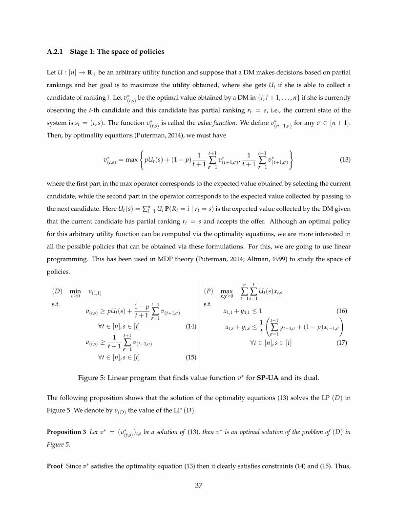
A.2.1 Stage 1: The space of policies

Let U : [n] → R+ be an arbitrary utility function and suppose that a DM makes decisions based on partial

rankings and her goal is to maximize the utility obtained, where she gets Ui if she is able to collect a

candidate of ranking i. Let v∗(t,s) be the optimal value obtained by a DM in {t, t + 1, . . . , n} if she is currently

observing the t-th candidate and this candidate has partial ranking rt = s, i.e., the current state of the

system is st = (t, s). The function v∗(t,s) is called the value function. We define v∗(n+1,σ) for any σ ∈ [n + 1].

Then, by optimality equations (Puterman, 2014), we must have

v∗(t,s) = max

{pUt(s) + (1− p)

1t + 1

t+1

∑σ=1

v∗(t+1,σ),1

t + 1

t+1

∑σ=1

v∗(t+1,σ)

}(13)

where the first part in the max operator corresponds to the expected value obtained by selecting the current

candidate, while the second part in the operator corresponds to the expected value collected by passing to

the next candidate. Here Ut(s) = ∑ni=1 Ui P(Rt = i | rt = s) is the expected value collected by the DM given

that the current candidate has partial ranking rt = s and accepts the offer. Although an optimal policy

for this arbitrary utility function can be computed via the optimality equations, we are more interested in

all the possible policies that can be obtained via these formulations. For this, we are going to use linear

programming. This has been used in MDP theory (Puterman, 2014; Altman, 1999) to study the space of

policies.

(D) minv≥0

v(1,1) (P) maxx,y≥0

n

∑t=1

t

∑s=1

Ut(s)xt,s

s.t.v(t,s) ≥ pUt(s) +

1− pt + 1

t+1

∑σ=1

v(t+1,σ)

∀t ∈ [n], s ∈ [t] (14)

v(t,s) ≥1

t + 1

t+1

∑σ=1

v(t+1,σ)

∀t ∈ [n], s ∈ [t] (15)

s.t.x1,1 + y1,1 ≤ 1 (16)

xt,s + yt,s ≤1t

(t−1

∑σ=1

yt−1,σ + (1− p)xt−1,σ

)∀t ∈ [n], s ∈ [t] (17)

Figure 5: Linear program that finds value function v∗ for SP-UA and its dual.

The following proposition shows that the solution of the optimality equations (13) solves the LP (D) in

Figure 5. We denote by v(D) the value of the LP (D).

Proposition 3 Let v∗ = (v∗(t,s))t,s be a solution of (13), then v∗ is an optimal solution of the problem of (D) in

Figure 5.

Proof Since v∗ satisfies the optimality equation (13) then it clearly satisfies constraints (14) and (15). Thus,

37

v∗ is feasible and so v∗(1,1) ≥ v(D).

To show the optimality of v∗, we show that any solution v of the LP is an upper bound for the value

function: v∗ ≤ v. To show this, we proceed by backward induction in t = n + 1, n, . . . , 1 and we prove that

v∗(t,s) ≤ v(t,s) for any s ∈ [t].

We start with the case t = n + 1. In this case v∗(n+1,s) = 0 for any s and since v(n + 1, s) ≥ 0 for any s, then

the result follows.

Suppose the result is true for t = τ + 1, . . . , n + 1 and let us show it for t = τ. Using Constraints (14)-(15)

we must have

v(τ,s) ≥ max

{pUτ(s) + (1− p)

1τ + 1

τ+1

∑σ=1

v(τ+1,σ),1

τ + 1

τ+1

∑σ=1

v(τ+1,σ)

}

≥ max

{pUτ(s) + (1− p)

1τ + 1

τ+1

∑σ=1

v∗(τ+1,σ),1

τ + 1

τ+1

∑σ=1

v∗(τ+1,σ)

}(backward induction)

= v∗(τ,s)

where the last line follows by the optimality equations (13). Thus, v(D) = v(1,1) ≥ v∗(1,1). �

The dual of the LP (D) is depicted in Figure 5 and named (P). The crucial fact to notice here is that the

feasible region of (P) is oblivious of the utility function (or rewards) given initially to the MDP. This suggest

that the region

POL =

{(x, y) ≥ 0 : x1,1 + y1,1 = 1, xt,s + yt,s =

1t

t−1

∑σ=1

(yt−1,σ + (1− p)xt−1,σ) , ∀t ∈ [n], s ∈ [t]

}

codifies all possible policies. The following two propositions formalize this.

Proposition 4 For any policy P for the SP-UA, consider xt,s = P(P reaches state (t, s), selects candidate) and

yt,s = P(P reaches state (t, s), does not select candidate). Then (x, y) belongs to POL.

Proof Consider the event Dt = {t-th candidate turns down offer}. Then p = P(Dt). Consider also the

events

Ot = {P reaches t-th candidate and extends an offer}

and

Ot = {P reaches t-th candidate and does not extend offer}.

38

Then Ot and Ot are disjoint events and Ot ∪Ot equals the event of P reaching stage t. Thus

1Ot∩{St=(t,s)} + 1Ot∩{St=(t,s)} = 1{P reaches state St=(t,s)}. (18)

Note that xt,s = P(Ot ∩ {St = (t, s)}) and yt,s = P(Ot ∩ {St = (t, s)}). For t = 1, then S1 = (1, 1) and

{P reaches state S1 = (1, 1)} occurs with probability 1. Thus

x1,1 + y1,1 = 1.

For t > 1, by the dynamics of the system, the only way that P reaches state t is by reaching stage t− 1 and

not extending an offer to the t− 1 candidate or extending an offer but this was turned down. Thus,

1{P reaches state St=(t,s)} =t−1

∑σ=1

1Ot−1∩{St−1=(t−1,σ)}∩{St=(t,s)} + 1Ot−1∩{St−1=(t−1,σ)}∩Dt−1∩{St=(t,s)} (19)

Note that

P(Ot−1 ∩ {St−1 = (t− 1, σ)} ∩ {St = (t, s)})

= P(Ot−1 ∩ {St−1 = (t− 1, σ)} | St = (t, s)) P(St = (t, s))

= P(Ot−1 ∩ {St−1 = (t− 1, σ)})1t

=1t

yt−1,σ.

Note that we use that P ’s action at stage t− 1 only depends on St−1 and not what is observed in the future.

Likewise we obtain

P(Ot−1 ∩ {St−1 = (t− 1, σ)} ∩ Dt−1 ∩ {St = (t, s)})

= P(Dt−1) P(Ot−1 ∩ {St−1 = (t− 1, σ)} ∩ {St = (t, s)})

= (1− p) P(Ot−1 ∩ {St−1 = (t− 1, σ)} ∩ {St = (t, s)})

=1− p

txt−1,σ.

Using the equality between (18) and (19) and taking expectation, we obtain

xt,s + yt,s =t−1

∑σ=1

1t

yt−1,σ +1− p

txt−1,σ

which shows that (x, y) ∈ POL. �

39

Conversely

Proposition 5 Let (x, y) be a point in POL. Consider the (randomized) policy P that in state (t, s) makes an offer

to the candidate t with probability x1,1 if t = 1 and

txt,s

∑t−1σ=1 yt−1,σ + (1− p)xt−1,σ

,

if t > 1. Then P is a policy for SP-UA such that xt,s = P(P reaches state (t, s), selects candidate) and yt,s =

P(P reaches state (t, s), does not select candidate) for any t ∈ [n] and s ∈ [t].

Proof We use the same events Ot, Ot and Dt as defined in the previous proof. Thus, we need to show that

xt,s = P(Ot ∩ {St = (t, s)}) and yt,s = P(Ot ∩ {St = (t, s)}) are the right marginal probabilities. For this, its

is enough to show that

P(Ot | St = (t, s)) = txt,s and P(Ot | St = (t, s)) = tyt,s

for any t ∈ [n] and for any s ∈ [t]. We prove this by induction in t ∈ [n]. For t = 1, the result is true by

definition of the acceptance probability and the fact that x1,1 + y1,1 = 1. Let us assume the result is true for

t− 1 and let us show it for t. First we have

P(Ot | St = (t, s)) = P(Reach t,P(St) = offer | St = (t, s))

= P(Reach t | St = (t, s)) P(P(St) = offer | St = (t, s))

= P(Reach t | St = (t, s)) · txt,s(∑t−1

σ=1 yt−1,σ + (1− p)xt−1,s

)

40

Now, we have

P(Reach t | St = (t, s)) = P((Ot−1 ∩ Dt−1) ∪Ot−1 | St = (t, s))

= (1− p)t−1

∑σ=1

P(Ot−1 | St−1 = (t− 1, σ), St = (t, s)) P(St−1 = (t− 1, σ) | St = (t, s))

+t−1

∑σ=1

P(Ot−1 | St−1 = (t− 1, σ), St = (t, s)) P(St−1 = (t− 1, σ) | St = (t, s))

= (1− p)t−1

∑σ=1

P(Ot−1 | St−1 = (t− 1, σ))1

t− 1

+t−1

∑σ=1

P(Ot−1 | St−1 = (t− 1, σ))1

t− 1

(P only makes decisions at stage t− 1 based on St−1)

= (1− p)t−1

∑σ=1

xt−1,σ + yt−1,σ (induction)

Note that we used

P(St−1 = (t− 1, σ) | St = (t, s)) =P(St = (t, s) | St−1 = (t− 1, σ)) P(St−1 = (t− 1, σ))

P(St = (t, s))=

1t− 1

.

Thus, the induction holds for P(Ot | St = (t, s)) = txt,s. Similarly, for

P(Ot | St = (t, s)) = P(Reach t,P(St) = pass | St = (t, s))

= P(Reach t | St = (t, s)) P(P(St) = pass | St = (t, s))

=

(t−1

∑σ=1

yt−1,σ + (1− p)xt−1,σ

)1− txt,s(∑t−1

σ=1 yt−1,σ + (1− p)xt−1,s

)

= tyt,s

where we used the fact that (x, y) ∈ POL. �

A.2.2 Stage 2: The robust objective

Proposition 6 Let P be any policy for SP-UA and let (x, y) ∈ POL be its corresponding vector as in Proposition 4.

Then, for any k ∈ [n],

P(P collects a top k candidate) =n

∑t=1

t

∑s=1

pxt,s P(Rt ≤ k | rt = s).

41

Proof We use the same events as in the proof of Proposition 4. Then,

P(P collects a top k candidate) =n

∑t=1

t

∑s=1

P(Ot ∩ Dt ∩ {St = (t, s)} ∩ {Rt ≤ k})

=n

∑t=1

t

∑s=1

pxt,s P(Rt ≤ k | Ot ∩ Dt ∩ {St = (t, s)})

=n

∑t=1

t

∑s=1

pxt,s P(Rt ≤ k | rt = s)

Note that Rt only depends on St and St = (t, s) is equivalent to rt = s. �

We are ready to prove of Theorem 2.

Theorem 6 (Theorem 2 restated) The largest robust ratio γ∗n corresponds to the optimal value of the LP

(LP)n,p

maxx≥0

γ

s.t.

xt,s ≤1t

(1− p

t−1

∑τ=1

τ

∑σ=1

xτ,σ

)∀t ∈ [n], s ∈ [t]

γ ≤ p1− (1− p)k

n

∑t=1

t

∑s=1

xt,s P(Rt ≤ k | rt = s) ∀k ∈ [n],

Moreover, given an optimal solution (x∗, γ∗n) of (LP)n,p, the (randomized) policy P∗ that at state (t, s) makes an offer

with probability tx∗t,s/(

1− p ∑t−1τ=1 ∑τ

σ=1 x∗τ,σ

)is γ∗n-robust.

Proof We have

γ∗n = maxP

mink∈[n]

P(P collects a candidate with rank ≤ k)1− (1− p)k

= max(x,y)∈POL

mink∈[n]

p ∑nt=1 ∑t

s=1 xt,s P(Rt ≤ k | rt = s)1− (1− p)k (Propositions 4, 5 and 6)

Now note that the function γ : (x, y) 7→ mink∈[n]p ∑n

t=1 ∑ts=1 xt,s P(Rt≤k|rt=s)1−(1−p)k is constant in y. Thus any point

(x, y) satisfying Constraints (16)-(17) has an equivalent point in (x′, y′) ∈ POL with x′ = x, y′ ≥ y so all

constraints tighten and the objective of γ is the same for both points. Thus, γ∗n equals the optimal value of

the LP (P′):

42

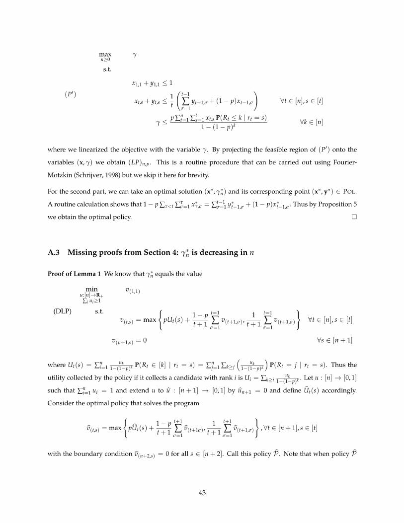
(P′)

maxx≥0

γ

s.t.

x1,1 + y1,1 ≤ 1

xt,s + yt,s ≤1t

(t−1

∑σ=1

yt−1,σ + (1− p)xt−1,σ

)∀t ∈ [n], s ∈ [t]

γ ≤ p ∑nt=1 ∑t

s=1 xt,s P(Rt ≤ k | rt = s)1− (1− p)k ∀k ∈ [n]

where we linearized the objective with the variable γ. By projecting the feasible region of (P′) onto the

variables (x, γ) we obtain (LP)n,p. This is a routine procedure that can be carried out using Fourier-

Motzkin (Schrijver, 1998) but we skip it here for brevity.

For the second part, we can take an optimal solution (x∗, γ∗n) and its corresponding point (x∗, y∗) ∈ POL.

A routine calculation shows that 1− p ∑τ<t ∑τσ=1 x∗τ,σ = ∑t−1

σ=1 y∗t−1,σ + (1− p)x∗t−1,σ. Thus by Proposition 5

we obtain the optimal policy. �

A.3 Missing proofs from Section 4: γ∗n is decreasing in n

Proof of Lemma 1 We know that γ∗n equals the value

minu:[n]→R+

∑i ui≥1

v(1,1)

(DLP) s.t.v(t,s) = max

{pUt(s) +

1− pt + 1

t=1

∑σ=1

v(t+1,σ),1

t + 1

t=1

∑σ=1

v(t+1,σ)

}∀t ∈ [n], s ∈ [t]

v(n+1,s) = 0 ∀s ∈ [n + 1]

where Ut(s) = ∑ni=1

uk1−(1−p)k P(Rt ∈ [k] | rt = s) = ∑n

j=1 ∑k≥j

(uk

1−(1−p)k

)P(Rt = j | rt = s). Thus the

utility collected by the policy if it collects a candidate with rank i is Ui = ∑k≥iuk

1−(1−p)k . Let u : [n] → [0, 1]

such that ∑ni=1 ui = 1 and extend u to u : [n + 1] → [0, 1] by un+1 = 0 and define Ut(s) accordingly.

Consider the optimal policy that solves the program

v(t,s) = max

{pUt(s) +

1− pt + 1

t+1

∑σ=1

v(t+1σ),1

t + 1

t+1

∑σ=1

v(t+1,σ)

}, ∀t ∈ [n + 1], s ∈ [t]

with the boundary condition v(n+2,s) = 0 for all s ∈ [n + 2]. Call this policy P . Note that when policy P

43

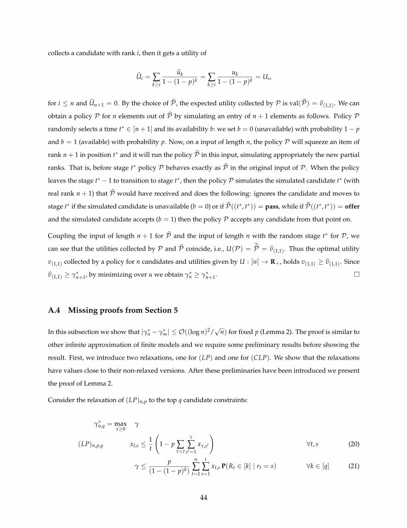
collects a candidate with rank i, then it gets a utility of

Ui = ∑k≥i

uk

1− (1− p)k = ∑k≥i

uk

1− (1− p)k = Ui,

for i ≤ n and Un+1 = 0. By the choice of P , the expected utility collected by P is val(P) = v(1,1). We can

obtain a policy P for n elements out of P by simulating an entry of n + 1 elements as follows. Policy P

randomly selects a time t∗ ∈ [n + 1] and its availability b: we set b = 0 (unavailable) with probability 1− p

and b = 1 (available) with probability p. Now, on a input of length n, the policy P will squeeze an item of

rank n + 1 in position t∗ and it will run the policy P in this input, simulating appropriately the new partial

ranks. That is, before stage t∗ policy P behaves exactly as P in the original input of P . When the policy

leaves the stage t∗ − 1 to transition to stage t∗, then the policy P simulates the simulated candidate t∗ (with

real rank n + 1) that P would have received and does the following: ignores the candidate and moves to

stage t∗ if the simulated candidate is unavailable (b = 0) or if P((t∗, t∗)) = pass, while if P((t∗, t∗)) = offer

and the simulated candidate accepts (b = 1) then the policy P accepts any candidate from that point on.

Coupling the input of length n + 1 for P and the input of length n with the random stage t∗ for P , we

can see that the utilities collected by P and P coincide, i.e., U(P) = P = v(1,1). Thus the optimal utility

v(1,1) collected by a policy for n candidates and utilities given by U : [n] → R+, holds v(1,1) ≥ v(1,1). Since

v(1,1) ≥ γ∗n+1, by minimizing over u we obtain γ∗n ≥ γ∗n+1. �

A.4 Missing proofs from Section 5

In this subsection we show that |γ∗n − γ∗∞| ≤ O((log n)2/√

n) for fixed p (Lemma 2). The proof is similar to

other infinite approximation of finite models and we require some preliminary results before showing the

result. First, we introduce two relaxations, one for (LP) and one for (CLP). We show that the relaxations

have values close to their non-relaxed versions. After these preliminaries have been introduced we present

the proof of Lemma 2.

Consider the relaxation of (LP)n,p to the top q candidate constraints:

γ∗n,q = maxx≥0

γ

(LP)n,p,q xt,s ≤1t

(1− p ∑

τ<t

τ

∑s′=1

xτ,s′

)∀t, s (20)

γ ≤ p(1− (1− p)k)

n

∑t=1

t

∑s=1

xt,s P(Rt ∈ [k] | rt = s) ∀k ∈ [q] (21)

44

Note that γ∗n ≤ γ∗n,q since (LP)n,p,q is a relaxation of (LP)n,p. The following result gives a bound on γ∗n

compared to γ∗n,q.

Proposition 7 For any q ∈ [n], γ∗n ≥ (1− (1− p)q) γ∗n,q.

Proof Let (x, γ∗n,q) be an optimal solution of (LP)n,p,q. Let fk = p1−(1−p)k ∑n

t=1 ∑ts=1 xt,s P(Rt ∈ [k] | rt =

s). Then γ∗n,q = mink=1,...,q fi. It is enough to show that fi ≥(

1−(1−p)q

1−(1−p)n

)fq for i ≥ q because γ∗n ≥

mini=1,...,n fi ≥(

1−(1−p)q

1−(1−p)n

)mini=1,...,q fi ≥ (1− (1− p)q) γ∗n,q.

For any j we have

f j+1 =p

1− (1− p)j+1

n

∑t=1

t

∑s=1

xt,s P(Rt ∈ [j + 1] | rt = s) ≥(

1− (1− p)j

1− (1− p)j+1

)f j.

Thus, iterating this for j > q we get f j ≥(

1−(1−p)q

1−(1−p)j

)fq and we obtain the desired result. �

Likewise we consider the relaxation of (CLP)p to the top q candidates:

γ∗∞,q = maxα:[0,1]×N→[0,1]

γ≥0

γ

(CLP)p,q α(t, s) ≤ 1t

(1− p

∫ t

0∑σ≥1

α(τ, σ)dτ

)∀t ∈ [0, 1], s ≥ 1

(22)

γ ≤ p(1− (1− p)k)

∫ 1

0∑s≥1

α(t, s)k

∑`=s

(`− 1s− 1

)ts(1− t)`−s dt ∀k ∈ [q] (23)

We have γ∗∞,q ≥ γ∗∞ and we have the approximate converse

Proposition 8 For any q ≥ 1, γ∗∞ ≥ (1− (1− p)q) γ∗∞,q.

Proof Let (α, γ∞,q) be a feasible solution of (CLP)p,q. Let

fk =p

1− (1− p)k

∫ 1

0∑s≥1

α(t, s)k

∑`=s

(`− 1s− 1

)ts(1− t)`−s dt

Assume that γ∞,q ≤ mink≤q fk. As in the previous proof, we aim to show that fi ≥ (1− (1− p)q) fq for

i ≥ q, since this will imply γ∗∞ ≥ (1− (1− p)q)γ∞,q for any (α, γ∞,q) feasible for (CLP)p,q.

45

Now, for any j we have

f j+1 =p

1− (1− p)j+1

∫ 1

0∑s≥1

α(t, s)j+1

∑`=s

(`− 1s− 1

)ts(1− t)`−s dt

≥ p1− (1− p)j+1

∫ 1

0∑s≥1

α(t, s)j

∑`=s

(`− 1s− 1

)ts(1− t)`−s dt

=

(1− (1− p)j

1− (1− p)j+1

)f j.

Iterating the inequality until reaching q we deduce that for any j ≥ q we have f j ≥(

1−(1−p)q

1−(1−p)j

)fq. From

here the result follows. �

Remark 2 If we set q = (log n)/p, both results imply that γ∗n ≥ (1− 1/n) γ∗n,q and γ∗∞ ≥ (1− 1/n) γ∗∞,q. Thus

we lose at most 1/n by restricting the analysis to the top q candidates.

Proposition 9 There is n0 such that for n ≥ n0, for any t such that√

n log n ≤ t ≤ n−√

n log n, ` ≤ log(n)/p

and ` ≥ s it holds that for any τ ∈ [t/n, (t + 1)/n] we have

1− 10p√

n≤

(`−1s−1)(

n−`t−s )/(

nt)

(`−1s−1)τ

s(1− τ)`−s≤ 1 +

10p√

n.

Proof We only need to show that

1− 10p√

n≤

(n−`t−s )/(

nt)

τs(1− τ)`−s ≤ 1 +10

p√

n.

We have

(n−`t−s )

(nt)

=t!

(t− s)!1n!

(n− `)!(n− t)!(n− t− (`− s))!

=

(t · (t− 1) · · · (t− s + 1)

n · (n− 1) · · · (n− s + 1)

)((n− t)(n− t− 1) · · · (n− t− (`− s) + 1)(n− s)(n− s− 1) · · · (n− s− (`− s) + 1)

)

=

(tn

)s (1− t

n

)`−s

︸ ︷︷ ︸A

1 ·(

1− 1t

)· · ·(

1− (s−1)t

)1 ·(

1− 1n

)· · ·(

1− (s−1)n

)

︸ ︷︷ ︸B

1 ·(

1− 1n−t

)· · ·(

1− (`−s)−1n−t

)(1− s

n)·(

1− (s+1)n

)· · ·(

1− (s+(`−s)−1)n

)

︸ ︷︷ ︸C

We bound terms A, B and C separately. Since s ≤ ` and we are assuming that ` ≤ (log n)/p and t ≥√

n log n for n large, then we will implicitly use that s, ` ≤ min{t/2, n/2}.

Claim A.1(1− 4/(p

√n))

τs(1− τ)`−s ≤ A = (t/n)s (1− t/n)`−s ≤(1 + 4/(p

√n))

τs(1− τ)`−s.

46

Proof For the upper bound we have

(tn

)s (1− t

n

)`−s≤ τs

(1− τ +

1n

)`−s(τ ∈ [t/n, (t + 1)/n])

= τs(1− τ)`−s(

1 +1

(1− τ)n

)`−s

≤ τs(1− τ)`−se(`−s)/((1−τ)n)

≤ τs(1− τ)`−se`/(n−t−1)

≤ τs(1− τ)`−s(

1 + 2`

n− t− 1

)(Using ex ≤ 1 + 2x for x ∈ [0, 1])

The upper bound now follows by using the information over ` and t and that (1 + 2`/(n− t− 1)) ≤ 1 +

2(log n)p−1(√

n log n− 1)−1 ≤ 1 + 4/(p√

n) for n large.

For the lower bound we have

(tn

)s (1− t

n

)`−s≥(

τ − 1n

)s(1− τ)`−s

= τs(1− τ)`−s(

1− 1τn

)s

≥ τs(1− τ)`−se−s

τn−1

≥ τs(1− τ)`−s (1− s/(τn− 1))

Since s/(τn− 1) ≤ log(n)/(p(t− 1)) ≤ 2/(p√

n) for n large, the lower bound follows. �

Claim A.2 1− 2s2/t ≤ B ≤ 1 + 2s2/n

Proof For the upper bound we upper bound the denominator

1 ·(

1− 1t

)· · ·(

1− (s−1)t

)1 ·(

1− 1n

)· · ·(

1− (s−1)n

) ≤ 1

1 ·(

1− 1n

)· · ·(

1− (s−1)n

)≤ e∑s−1

k=1 k/(n−k)

≤ es2/n (Function x 7→ x/(n− x) is increasing)

≤ 1 + 2s2

n

47

For the lower bound we lower bound the numerator:

1 ·(

1− 1t

)· · ·(

1− (s−1)t

)1 ·(

1− 1n

)· · ·(

1− (s−1)n

) ≥ 1 ·

(1− 1

t

)· · ·(

1− (s− 1)t

)

≥ e−∑s−1k=1 k/(t−k) (Using 1− k/t = (1 + k/(t− k))−1 ≥ e−k/(t−k))

≥ 1− s2

t− s≥ 1− 2

s2

t.

�

Claim A.3 1− 2`2/(n− t) ≤ C ≤ 1 + 2`2/n

Proof Similar to the previous claim, we bound denominator for an upper bound and numerator for a lower

bound.

1 ·(

1− 1n−t

)· · ·(

1− (`−s)−1n−t

)(1− s

n)·(

1− (s+1)n

)· · ·(

1− (s+(`−s)−1)n

) ≤ 1(

1− sn)·(

1− (s+1)n

)· · ·(

1− (s+(`−s)−1)n

)≤ e∑`−s−1

k=0 (k+s)/(n−k) ≤ 1 + 2`2

n,

and

1 ·(

1− 1n−t

)· · ·(

1− (`−s)−1n−t

)(1− s

n)·(

1− (s+1)n

)· · ·(

1− (s+(`−s)−1)n

) ≥ 1 ·

(1− 1

n− t

)· · ·(

1− (`− s)− 1n− t

)

≥ e−∑`−s−1k=0 k/(n−t−k) ≥ 1− 2

`2

n− t.

�

We can now upper bound ABC as

ABC ≤ τs(1− τ)`−s(

1 +4

p√

n

)(1 + 2

s2

n

)(1 + 2

`2

n

)≤ τs(1− τ)`−s

(1 +

4p√

n

)(1 + 2

(log n)2

p2n

)2

(Using t ≤ n−√

n log n and s ≤ ` ≤ (log n)/p)

≤ τs(1− τ)`−s(

1 +4

p√

n

)(1 + 6

(log n)2

p2n

)(Using (1 + x)2 ≤ 1 + 3x if x ∈ [0, 1])

≤ τs(1− τ)`−s(

1 +10

p√

n

).

48

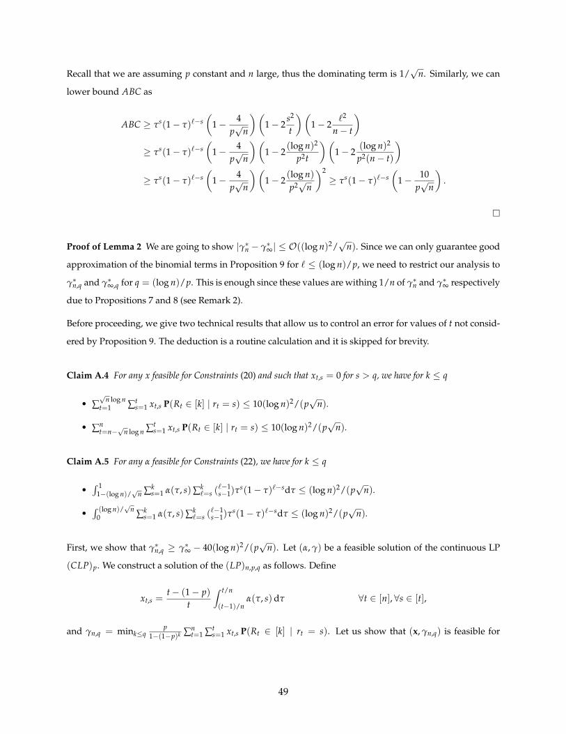
Recall that we are assuming p constant and n large, thus the dominating term is 1/√

n. Similarly, we can

lower bound ABC as

ABC ≥ τs(1− τ)`−s(

1− 4p√

n

)(1− 2

s2

t

)(1− 2

`2

n− t

)≥ τs(1− τ)`−s

(1− 4

p√

n

)(1− 2

(log n)2

p2t

)(1− 2

(log n)2

p2(n− t)

)≥ τs(1− τ)`−s

(1− 4

p√

n

)(1− 2

(log n)p2√

n

)2

≥ τs(1− τ)`−s(

1− 10p√

n

).

�

Proof of Lemma 2 We are going to show |γ∗n − γ∗∞| ≤ O((log n)2/√

n). Since we can only guarantee good

approximation of the binomial terms in Proposition 9 for ` ≤ (log n)/p, we need to restrict our analysis to

γ∗n,q and γ∗∞,q for q = (log n)/p. This is enough since these values are withing 1/n of γ∗n and γ∗∞ respectively

due to Propositions 7 and 8 (see Remark 2).

Before proceeding, we give two technical results that allow us to control an error for values of t not consid-

ered by Proposition 9. The deduction is a routine calculation and it is skipped for brevity.

Claim A.4 For any x feasible for Constraints (20) and such that xt,s = 0 for s > q, we have for k ≤ q

• ∑√

n log nt=1 ∑t

s=1 xt,s P(Rt ∈ [k] | rt = s) ≤ 10(log n)2/(p√

n).

• ∑nt=n−

√n log n ∑t

s=1 xt,s P(Rt ∈ [k] | rt = s) ≤ 10(log n)2/(p√

n).

Claim A.5 For any α feasible for Constraints (22), we have for k ≤ q

•∫ 1

1−(log n)/√

n ∑ks=1 α(τ, s)∑k

`=s (`−1s−1)τ

s(1− τ)`−sdτ ≤ (log n)2/(p√

n).

•∫ (log n)/

√n

0 ∑ks=1 α(τ, s)∑k

`=s (`−1s−1)τ

s(1− τ)`−sdτ ≤ (log n)2/(p√

n).

First, we show that γ∗n,q ≥ γ∗∞ − 40(log n)2/(p√

n). Let (α, γ) be a feasible solution of the continuous LP

(CLP)p. We construct a solution of the (LP)n,p,q as follows. Define

xt,s =t− (1− p)

t

∫ t/n

(t−1)/nα(τ, s)dτ ∀t ∈ [n], ∀s ∈ [t],

and γn,q = mink≤qp

1−(1−p)k ∑nt=1 ∑t

s=1 xt,s P(Rt ∈ [k] | rt = s). Let us show that (x, γn,q) is feasible for

49

(LP)n,q, i.e., it satisfies Constraints (20)-(21). First, for τ ∈ [(t− 1)/n, t/n] we have

τα(τ, s) + p∫ τ

(t−1)/nα(τ′, s)dτ′ ≤ 1− p

∫ τ

0∑σ≥1

α(τ′, σ)dτ′ + p∫ τ

(t−1)/nα(τ′, s)dτ′

≤ 1− p∫ (t−1)/n

0∑σ≥1

α(τ′, σ)dτ′ ≤ 1− pt−1

∑τ′=1

τ′

∑σ=1

xτ′ ,σ.

We now integrate in [(t− 1)/n, t/n] on both sides of the inequality. After integration, the RHS equals(1− p ∑t

τ=1 ∑τσ=1 xτ,σ

)/n. On the LHS we obtain,

∫ t/n

(t−1)/n

(τα(τ, s) + p

∫ τ

(t−1)/nα(τ′, s)dτ′

)dτ =

tn

∫ t/n

(t−1)/nα(τ, s)dτ − (1− p)

∫ t/n

(t−1)/n

(tn− τ

)α(τ, s)dτ

≥ (t− (1− p))n

∫ t/n

(t−1)/nα(τ, s)dτ (Using t/n− τ ≤ 1/n)

=tn

xt,s.

Thus Constraints (20) hold. By definition of γn,q, Constraints (21) also hold.

Now, note that for t ≥√

n log n we have

xt,s ≥(

1− 1√n log n

) ∫ t/n

(t−1)/nα(τ, s)dτ.

Then,

γn,q = mink≤q

p1− (1− p)k

n

∑t=1

t

∑s=1

xt,s

k∧(n−t+s)

∑`=s

(`−1s−1)(

n−`t−s )

(nt)

(Definition of P(Rt ∈ [k] | rt = s))

≥ mink≤q

p1− (1− p)k

n−√

n log n

∑t=√

n log n

t

∑s=1

∫ t/n

(t−1)/nα(τ, s)dτ

k∧(n−t+s)

∑`=s

(`−1s−1)(

n−`t−s )

(nt)

(1− 1√

n log n

)

≥ mink≤q

p1− (1− p)k

n−√

n log n

∑t=√

n log n

k

∑s=1

∫ t/n

(t−1)/nα(τ, s)

k

∑`=s

(`− 1s− 1

)τs(1− τ)`−s dτ

(1− 20

p√

n

)(Since n− t + s ≥

√n log n ≥ k and t ≤ k and using Proposition 9)

= mink≤q

p1− (1− p)k

n−√

n log n

∑t=√

n log n

∫ t/n

(t−1)/n

k

∑`=1

`

∑s=1

α(τ, s)(`− 1s− 1

)τs(1− τ)`−s dτ

(1− 20

p√

n

)

≥ mink≤q

(p

1− (1− p)k

∫ 1

0

k

∑`=1

`

∑s=1

α(τ, s)(`− 1s− 1

)τs(1− τ)`−s dτ − 2

(log n)2

p√

n

)(1− 20

p√

n

)(Claim A.5)

≥(

γ− 2(log n)2

p√

n

)(1− 10

p√

n

)≥ γ− 20

p√

n− 2

log n√n

.

50

Optimizing over γ, γn,q and using Proposition 7 gives us γ∗n,q ≥ γ∗∞ − 40log(n)/(

p√

n)

for n large.

Now we show that γ∗∞,q ≥ γ∗n,q − 40(log n)2/(p√

n). Let (x, γn,q) be a solution of (LP)n,p,q. Let us construct

a solution of (CLP)p,q. Note that we can assume xt,s = 0 for s > q as (LP)n,p,q does not improve its objective

function by allocating any mass to these variables. Consider α defined as follows: for τ ∈ [0, 1] let

α(τ, s) =

nxt,s

(1− log(n)/

√n)

t = dτne ≥√

n, s ≤ min{t, log n/p}

0 t = dτne <√

n or s > min{t, log n/p}

Let γ∞,q = mink≤qp

1−(1−p)k

∫ 10 ∑s≥1 α(τ, s)∑k

`=s (`−1s−1)τ

s(1− τ)`−s dτ. We show first that (α, γ∞,q) is feasible

for (CLP)p,q, and for this it is enough to show that α holds Constraints (20). For τ < 1/√

n we have

α(τ, s) = 0 for any s, thus Constraint (22) is satisfied in this case. Let us verify that for τ ≥ 1/√

n the

constraint also holds. Let t = dτne and s ≥ 1. Then

τα(τ, s) + p∫ τ

0∑σ≥1

α(τ′, σ)dτ′ ≤ τα(τ, s) + pt−1

∑t′=1

∫ t′n

t′−1n

t′

∑s=1

α(τ′, s)dτ′ + p∫ τ

t−1n

log np

∑σ=1

α(τ′, σ)dτ′

≤(

1− log n√n

)(txt,s + p

t−1

∑t′=1

t′

∑s=1

xt′ ,s + plog n

pt

)(Since xt,s ≤ 1

t always)

≤(

1− log n√n

)(1 +

log nt

)≤(

1− log n√n

)(1 +

log n√n

). (t ≥

√n)

51

The last term is < 1. Thus (α, γ∞,q) is feasible for (CLP)p,q. Now,

γ∞,q = mink≤q

p1− (1− p)k

∫ 1

0∑s≥1

α(τ, s)k

∑`=s

(`− 1s− 1

)τs(1− τ)`−s dτ

≥ mink≤q

p1− (1− p)k

n−√

n log n

∑t=√

n log n

∫ tn

t−1n

∑s≥1

α(τ, s)k

∑`=s

(`− 1s− 1

)τs(1− τ)`−s dτ

≥ mink≤q

p1− (1− p)k

n−√

n log n

∑t=√

n log n

∫ tn

t−1n

∑s≥1

α(τ, s)k

∑`=s

(`−1s−1)(

n−`t−s )

(nt)

dτ

(1− 10

p√

n

)(Proposition 9)

≥ mink≤q

p1− (1− p)k

n−√

n log n

∑t=√

n log n

t

∑s=1

xt,s

k

∑`=s

(`−1s−1)(

n−`t−s )

(nt)

dτ

(1− log n√

n

)(1− 10

p√

n

)

≥(

mink≤q

p1− (1− p)k

n

∑t=1

t

∑s=1

xt,s

k

∑`=s

(`−1s−1)(

n−`t−s )

(nt)

dτ − 20(log n)2

p√

n

)(1− log n√

n

)(1− 10

p√

n

)(Claim A.4)

≥ γn,q − 40(log n)2

p√

n.

Thus optimizing over γ∗∞,q, γ∗n,q we obtain the desired bound. Using Propositions 7 and 8 we can conclude

that, for n large, γ∗∞ − 50(log n)2/(

p√

n)≤ γ∗n ≤ γ∗∞ + 50(log n)2/

(p√

n). �

A.5 Missing proofs from Section 6

Proof of Lemma 3 The input of the i.i.d. prophet inequality problem corresponds to a known distribution

D with support in [0, 1]. The DM sequentially accesses at most m samples from D and upon observing one

of these values, she has to decide irrevocably if to take it and stop the process or continue. We are going

to use A to design a strategy for the prophet problem. We assume that the samples from D are all distinct.

Indeed, we can add some small Gaussian noise to the distribution and consider a continuous distribution

D′ instead.

Note that A runs on an input of size n where a fraction p of the candidates accept an offer. We interpret

pn ≈ m as the set of samples for the prophet inequality problem, while the remaining (1− p)n items are

used as additional information for the algorithm. By concentration bounds, we are going to argue that we

only need to run A in at most (1 + ε)pn positive samples.

Formally, we proceed as follows. Fix n and ε > 0 and consider the algorithm B that receives an online

input of n numbers x1, . . . , xn. The algorithm flips n coins with probability of heads p and marks item i as

52

available if the corresponding coins that turn out heads. Algorithm B feeds algorithm A with the partial

rankings given by the ordering given by x1, . . . , xn. If A selects a candidate but the candidate is mark as

unavailable, then B moves to the next item. If A selects a candidate i and it is marked as available, then the

process ends with B collecting the value xi. Let us denote by Val(B, x1, . . . , xn) the value collected by B in

the online input x1, . . . , xn. Then we have the following claim.

Claim A.6 EX1,...,XnS

[Val(B, X1, . . . , Xn)] ≥ γ EX1,...,XnS

[maxi∈S Xi], where S is the random set of items marked as

available and X1, . . . , Xn are n i.i.d. random variables with common distribution D.

Proof Fix x1, . . . , xn points in the support of D. Then, a simple application of Proposition 1 shows

ES,π

[Val(B, xπ(1), . . . , xπ(n))

]ES [maxi∈S xi]

≥ γ

Note that we need to feed B with all permutations of x1, . . . , xn in order to obtain the guarantee of A. From

here, we obtain ES ,π [Val(B, xπ(1), . . . , xπ(n))] ≥ γ ES [maxi∈S xi] and the conclusion follows by taking

expectation in X1 = x1, . . . , Xn = xn. �

For ease of notation, we will refer by Val(·) to Val(·, X1, . . . , Xn). We modify slightly B. Consider B′ that

runs normally B if |S| ≤ (1 + ε)pn or simply return 0 value if |S| > (1 + ε)pn. Then, we have

Claim A.7 Let ε, δ > 0. For n ≥ 2 log (2/δ) /(pε2) we have EX1,...,XnS

[maxi/∈S Xi] ≥ (1− δ) E

[max

i≤(1−ε)pnXi

]and E [Val(B′)] + δ ≥ E [Val(B)].

Proof Using standard Chernoff concentration bounds (see for instance (Boucheron et al., 2013)) we get

PS (||S| − pn| ≥ εpn) ≤ 2e−pnε2/2 = δ. Hence, for n ≥ 2 log (2/δ) /(pε2), we can guarantee that

EX1,...,XnS

[maxi∈S

Xi

]≥ (1− δ) E

[max

i≤(1−ε)pnXi

].

For the second part we have E [Val(B)] ≤ δ + E [Val(B) | |S| ≤ (1 + ε)pn] = δ + E [Val(B′)]. �

Claim A.8 For any ε > 0 we have E

[max

i≤(1−ε)pnXi

]≥ (1− ε)2 E

[max

i≤(1+ε)pnXi

].

53

Proof Since P (maxi≤k Xi ≤ x) = P(X1 ≤ x)k, then we have

E

[max

i≤(1−ε)pnXi

]

E

[max

i≤(1+ε)pnXi

] =

∫ ∞0

(1− P(X1 ≤ x)pn(1−ε)

)dx∫ ∞

0

(1− P(X1 ≤ x)pn(1+ε)

)dx≥ inf

x≥0

1− P(X1 ≤ x)pn(1−ε)

1− P(X1 ≤ x)pn(1+ε)≥ inf

v∈[0,1)f (v)

where f (v) = (1− v1−ε)/(1− v1+ε). Now the conclusion follows by using the fact that the function f is

nonincreasing and that infv∈[0,1) f (v) = limv→1 f (v) = (1− ε)/(1 + ε) ≥ (1− ε)2. �

Putting together these two claims, we obtain an algorithm that checks at most (1 + ε)pn items and guaran-

tees

γ(1− ε)2(1− δ) E

[max

i≤(1+ε)pnXi

]≤ E

[Val(B′)

]+ δ.

Now, fix ε > 0 small enough such that (1 + ε)p < 1. We know that the set {b(1 + ε)pnc}n≥1 contains all

non-negative integers. Thus, for n ≥ 2 log (2/δ) /(pε2) algorithm B′ in an input of length m = b(1 + ε)pnc

guarantees

γ(1− ε)2(1− δ) E[

maxi≤m

Xi

]≤ E

[Val(B′)

]+ δ.

for any distribution D with support in [0, 1]. This finishes the proof. �

The next result uses notation from the work by Hill & Kertz. For the details we refer the reader to the

work (Hill and Kertz, 1982). The result states that there is a hard instance for the i.i.d. prophet inequality

problem where E[maxi≤m Xi] is away from 0 by a quantity at least 1/m3. The importance of this reformu-

lation of the result by Hill & Kertz is that e−Θ(n)/ E[maxi≤m Xi] → 0 which is what we needed to show

that γ ≤ 1/β. Recall that β ≈ 1.341 is the unique solution of the integral equation∫ 1

0 (y(1− log y) + β−

1)−1dy = 1 (Kertz, 1986).

Proposition 10 (Reformulation of Proposition 4.4 by Hill and Kertz (1982)) Let am be the sequence constructed

by Hill & Kertz, i.e, such that am → β and for any sequence of i.i.d. random variables X1, . . . , Xm with support in

[0, 1] we have

E[

maxi≤m

Xi

]≤ am sup {E[Xt] : t ∈ Tm} ,

where Tm is the set of stopping rules for X1, . . . , Xm. Then, for m large enough, there is a sequence of random variables

X1, . . . , Xm such that

• E[maxi≤m Xi

]≥ 1/m3, and

54

• E[maxi≤m Xi

]≥ (am − 1/m3) sup

{E[Xt] : t ∈ Tm

}.

Proof In Proposition 4.4 (Hill and Kertz, 1982), it is shown that that for any ε′ sufficiently small, there is

a random variable X with p0 = P(X = 0), pj = P(X = Vj(X)) for j = 0, . . . , m− 2, P(X = Vm−1(X)) =

pm−1− ε′ and P(X = 1) = ε′ such that E[maxi≤m Xi] ≥ (am− ε′) sup{

E[Xt] : t ∈ Tm

}, where X1, . . . , Xm are

m independent copies of X. Here Vj(X) = E[X ∧ E[Vj−1(X)]] corresponds to the optimal value computed

via dynamic programming and one can show that sup{

E[Xt] : t ∈ Tm

}= Vm(X) (see Lemma 2.1 in (Hill

and Kertz, 1982)). We only need to show that we can choose ε′ = 1/m3. The probabilities p0, . . . , pm−1 are

computed as follows: Let sj = (ηj,m(αm))1/m for j = 1, . . . , n− 2 where αm ∈ (0, 1) is the (unique) solution

of ηm−1,m(αm) = 1, then p0 = s0, pj = sj − sj−1 for j = 1, . . . , n− 2 and pn−1 = 1− sn−2. One can show that

sm−2 = (1− 1/m)1/(m−1) (1− αm/m)1/(m−1) and αm holds 1/(3e) ≤ αm ≤ 1/(e− 1) (see Proposition 3.6

in (Hill and Kertz, 1982)). For m large we have

e−1/(m−1) ≤ sm−2 ≤ e−1/(3em2)

then pm−1 = 1− sm−2 ≥ 1− e−1/(m−1) ≥ 1/m2 for m large. Thus we can set ε′ = 1/m3 and pm−1 − ε′ > 0

and the rest of the proof follows. Furthermore, E[maxi≤m Xi] ≥ ε′ · 1 ≥ 1/m3. �

A.6 Missing proofs from Section 7

Proof of Lemma 4 For p ≥ p∗ and ` = 0, 1, . . . , 4, we calculate tight lower bounds for the expression in the

letf-hand side of the inequality in the claim, and we show that these lower bounds are at least one, with the

lower bound attaining equality with 1 for ` = 1, 2. For ` ≥ 5 we can generalize the previous bounds and

show a universal lower bound of at least 1.

• For ` = 0, we have

∫ 1

p1/(1−p)

1tp dt =

11− p

(1− p) = 1 = (1− p)0.

• For ` = 1, we have

∫ 1

p1/(1−p)

(1− t)tp dt = 1−

∫ 1

p1/(1−p)t1−p dt = 1− 1

2− p

(1− p(2−p)/(1−p)

).

The last value is at least 1− p if an only if p(2− p) ≥ 1− p(2−p)/(1−p) iff p(2−p)/(1−p) ≥ (1− p)2. The

last inequality holds iff p ≥ p∗ ≈ 0.594134 where p∗ is computed numerically by solving (1− p)2 =

55

p(2−p)/(1−p).

• For ` = 2, we use the approximation p1/(1−p) ≤ (1 + p)/(2e) that follows from the concavity of the

function p1/(1−p) and the first-order approximation of the function at p = 1. With this we can lower

bound the integral

∫ 1

p1/(1−p)

(1− t)2

tp dt ≥∫ 1

(1+p)/(2e)

(1− t)2

tp dt

=∫ 1−(1+p)/(2e)

0u2(1− u)−p du (change of variable u = 1− t)

≥∫ 1−(1+p)/(2e)

0u2(

1 + pu + p(p + 1)u2

2

)du

(Using the series (1− u)−p = ∑k≥0 (−pk )(−u)k)

=13

(1− 1 + p

2e

)3+

p4

(1− 1 + p

2e

)4+

p(p + 1)10

(1− 1 + p

2e

)5.

By solving the polynomial we see that the last expression is ≥ (1− p)2 if and only if p ≥ 0.585395, thus

the inequality holds for p ≥ p∗.

• For ` = 3, 4 we can use a similar approach to get

∫ 1

p1/(1−p)

(1− p)`

tp dt ≥ 1`+ 1

(1− 1 + p

2e

)`+1+

p`+ 2

(1− 1 + p

2e

)`+2.

The last expression is ≥ (1− p)` for ` = 3, 4 if and only if p ≥ 0.559826.

• For ` ≥ 5, we have

∫ 1

p1/(1−p)

(1− t)`

tp dt ≥ (1− (1 + p)/(2e))`+1

`+ 1.

We aim to show that (1− (1 + p)/(2e))`+1/(`+ 1) ≥ (1− p)`. This is equivalent to show that(

1−(1+p)/(2e)1−p

)` (1− 1+p

2e

)≥

`+ 1.

Note that the function f (p) = (1− (1 + p)/(2e))/(1− p) is increasing since f ′(p) = (1− 1/e)/(1− p)2 >

0. For p = (2e− 1)/(4e− 3) ≈ 0.56351 we have f (p) = 2− 1/e. Thus for p ≥ p∗ > p and ` = 5 we have

f (p)5 (1− (1 + p)/(2e)) ≥ (2− 1/e)5(1− 1/e) ≥ 7.32 ≥ 6. By an inductive argument, we can show that

f (p)` (1− (1 + p)/(2e)) ≥ `+ 1 for any ` ≥ 5 and this finishes the proof.

�

56