ROBUST CONTROL FOR AN UNCERTAIN CHEMOSTAT MODEL … · ROBUST CONTROL FOR AN UNCERTAIN CHEMOSTAT MODEL JEAN{LUC GOUZE AND GONZALO ROBLEDO Abstract. In this paper we consider a control

ROBUST CONTROL FOR AN UNCERTAIN CHEMOSTAT

MODEL

JEAN–LUC GOUZE AND GONZALO ROBLEDO

Abstract. In this paper we consider a control problem for an uncertainchemostat model with a general growth function and cell mortality. Thisuncertainty affects the model (growth function) as well as the outputs (mea-surements of substrate). Despite this lack of information, an upper bound anda lower bound for those uncertainties are assumed to be known a priori. Webuild a family of feedback control laws on the dilution rate, giving a guaran-teed estimation on the unmeasured variable (biomass), and stabilizing the twovariables in a rectangular set, around a reference value of the substrate. Wegive two realistic applications of this control law to a depollution process andto phytoplankton culture.

1. Introduction

The chemostat is a continuous bioreactor used to culture microorganisms withconcentration x which consume a substrate s to grow. Mathematical modelingof chemostat has been extensively developed, mainly using ordinary differentialequations, and several results have been validated experimentally. See [1],[22] for areview of mathematical results on the theory of chemostat.

Feedback control of bioreactor models has been a focus of intensive research[1],[6],[9]; the problem we investigate in this paper deals with the feedback stabi-lization of an uncertain chemostat model. In this control context, uncertainty mustbe understood in two basic types:

(1) Internal : Some parts of the model are not precisely known; for examplethe functions that describe the kinetic reactions or some parameters.

(2) External : The measure of the variables is susceptible to undergo differentkinds of noise such as unknown additive or multiplicative disturbances.

We shall present two examples of robust stabilization of an uncertain chemostat:The first one is a water depollution process and the second one is the culture ofphytoplankton and the simulation of marine environments.

• We can consider the chemostat as a simple wastewater plant (see for exam-ple [21],[24]), where a selected microorganism x consumes a contaminant sand is expected to make decrease its concentration toward an acceptablelevel given by environmental laws. This goal is considerably complicatedby uncertainties of the kinetic model and the output.

• Chemostat has been used currently in marine laboratories (see [2],[3]) tosimulate in vitro the growth of unicellular phytoplanktonic algae in marine

Date: 4 August 2005.1991 Mathematics Subject Classification. 34D23,34H05,93B52.Key words and phrases. Chemostat, Uncertain models, Feedback control, Monotone systems.

1

2 GOUZE AND ROBLEDO

ecosystems, where the phytoplankton feeds on limiting substrate (e.g. ni-trate, iron, silicon, etc.) supplied at a constant rate. As it is easy to see,the standard equilibrium point in a chemostat with a monotone classicalgrowth function as the Michaelis–Menten function corresponds to a lowlevel of substrate: it comes from the fact that the growth function has alarge slope at the origin, attaining very fast its maximum. In fact, exper-imentally, the value of the substrate at the equilibrium is often so smallthat it is non measurable with the usual apparatus. To reproduce growthconditions with a high level of nutrient in vitro, we wish to be able tomaintain a high level of substrate at the equilibrium. At this level, the riskof washout (loss of biomass) is very high if there are uncertainties in themodel. Therefore we need a control to stabilize the chemostat and avoidwashout.

Feedback stabilization of a chemostat becomes nontrivial if we take into accountthat the model is inaccurate, thus the real dynamics is ill–known and the outputavailable is corrupted by noise.

Feedback stabilization of nonlinear uncertain systems [4],[15] deals with severalapproaches: e.g. deterministic, stochastic, adaptive control, etc: in [4] it is supposedthat the behavior of the uncertainties can be described by differential equations.Stochastic control (see [15, Ch.4]) supposes that the uncertainties satisfy somestatistical properties. In this article we will only suppose that the uncertainties aredeterministic and bounded.

An interesting deterministic issue for this stabilization problem has been givenin the framework of the game–theoretical control theory (see e.g. [14]). Roughlyspeaking, it assumes that the real system is not known to us, but there existsa (relatively wide) class of admissible systems, including the real one. This as-sumption implies that, given a stabilization objective, it must be satisfied for anysystem too. This idea has been complemented with a worst case approach (see[7],[8],[17],[19],[20]) by using the fact that (under some transformation of variables)a system Σ (e.g. bioreactor equations) can be studied using monotone dynami-cal systems theory [23]. Moreover, supposing that the bounds of uncertainties areknown a priori, a couple of well known systems (Σ−, Σ+) verifying the inequalityΣ− ≤ Σ ≤ Σ+ (in a sense that will be explained later on) is built. Hence, insteadof satisfying a feedback stabilization objective for any admissible system, we willneed only to satisfy this one for the “bounds” of the admissible systems.

Using these systems (Σ−, Σ+), interval observers for uncertain bioreactor modelshave been developed in [7],[8],[19],[20], allowing a partial estimation for the non-measured variables. Moreover, in [20] a feedback stabilization law is built usingthese interval observers. In almost all those articles (except [19]) it is supposedthat the output available is unperturbed and the mortality rate of the biomass(es)is negligible. This last assumption is one key step in reducing many chemostatmodels to a monotone dynamical systems where strong convergence properties arein evidence.

In this paper, we assume that the output undergoes multiplicative disturbances.Moreover, we drop the assumption of neglecting the mortality rate. Nevertheless,we are able to follow the ideas stated above, arriving to stabilize the uncertainchemostat without using interval observers.

ROBUST CONTROL FOR CHEMOSTAT MODELS 3

This paper is organized as follows: in section 2 we recall some facts of thechemostat model and state the assumptions about uncertainty. Section 3 presentsthe robust regulation problem in detail. The main result and its proof is given insection 4. The application and simulations are given in section 5.

2. Modeling of an uncertain chemostat

Let us recall the chemostat equations (see, for example [22, Chapt.1]):

(1)

s = D(sin − s) − αxf(s),

x = x(f(s) − D − m).

Where s(t) and x(t) are the concentration of the nutrient and the density of thebiomass at time t, sin > 0 denotes the input concentration of nutrient (in this paperwe will suppose that is a constant), D > 0 is the dilution rate, α > 0 is a growthyield constant. The function f : R+ 7→ R+ represents the per capita growth rateof nutrient of the biomass and m > 0 is the mortality rate. In general, the mor-tality rate is neglected and a “conservation law” for total biomass implies that theweighted sum of microbial concentration and substrate concentration equilibrates.Hence, the substrate equation can be asymptotically eliminated.

Chemostat is called also CSTR (continuous stirred tank reactor) because, as wecan deduce from system (1), the rate of the input flow is the same as that the rateof the output flow. We will assume that initial conditions of system (1) are in thebox [s−0 , s+

0 ] × [x−

0 , x+0 ] ⊂ Ω, where the set Ω is defined by:

Ω =(s, x) ∈ R

2+ : 0 < s < sin, x > 0 and s + αx + sin < v∗

where v∗ is a constant related to the volume of the chemostat.Now, we make the assumptions about uncertainty of chemostat model:

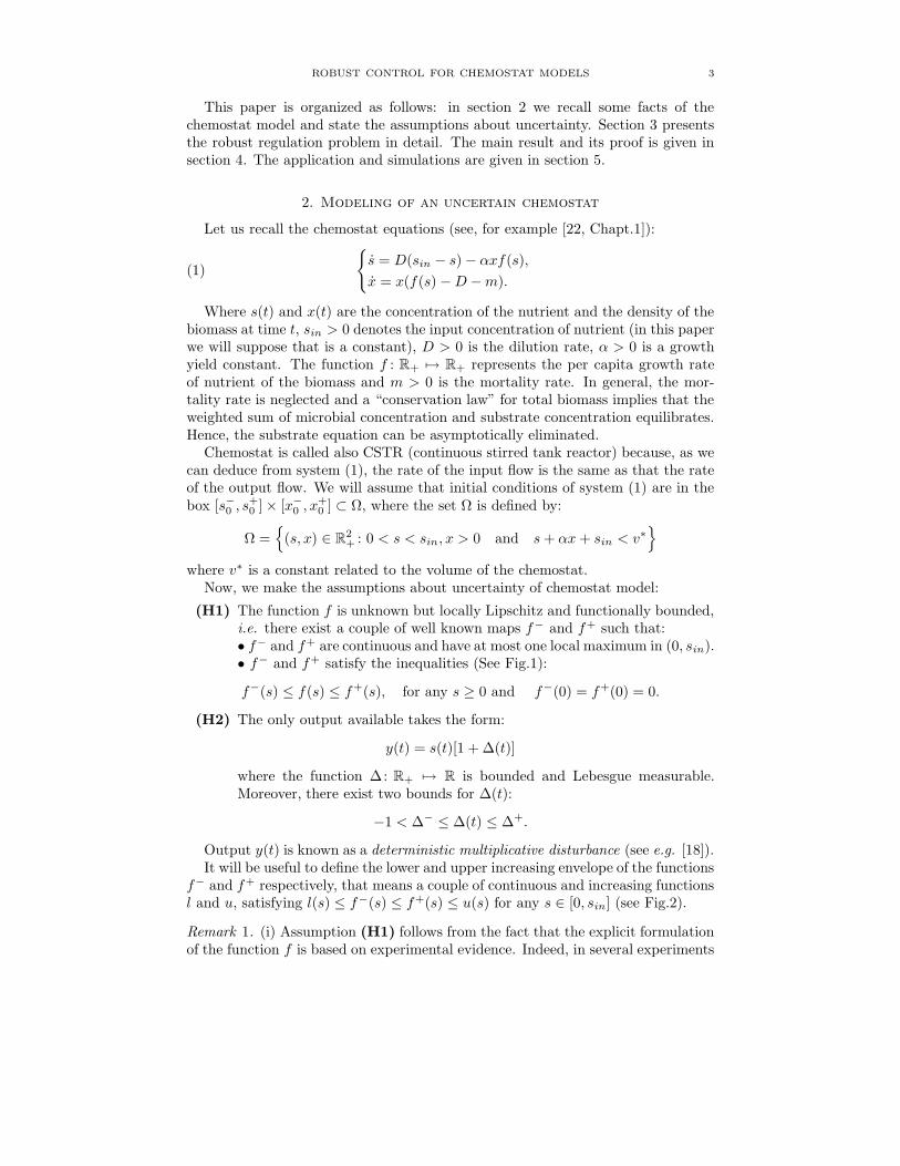
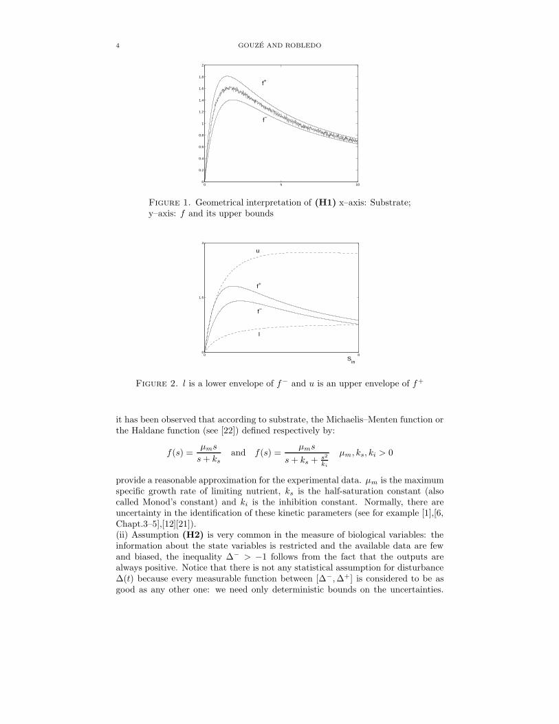
(H1) The function f is unknown but locally Lipschitz and functionally bounded,i.e. there exist a couple of well known maps f− and f+ such that:• f− and f+ are continuous and have at most one local maximum in (0, sin).• f− and f+ satisfy the inequalities (See Fig.1):

f−(s) ≤ f(s) ≤ f+(s), for any s ≥ 0 and f−(0) = f+(0) = 0.

(H2) The only output available takes the form:

y(t) = s(t)[1 + ∆(t)]

where the function ∆: R+ 7→ R is bounded and Lebesgue measurable.Moreover, there exist two bounds for ∆(t):

−1 < ∆− ≤ ∆(t) ≤ ∆+.

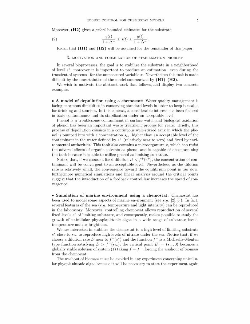
Output y(t) is known as a deterministic multiplicative disturbance (see e.g. [18]).It will be useful to define the lower and upper increasing envelope of the functions

f− and f+ respectively, that means a couple of continuous and increasing functionsl and u, satisfying l(s) ≤ f−(s) ≤ f+(s) ≤ u(s) for any s ∈ [0, sin] (see Fig.2).

Remark 1. (i) Assumption (H1) follows from the fact that the explicit formulationof the function f is based on experimental evidence. Indeed, in several experiments

4 GOUZE AND ROBLEDO

0 5 100

0.2

0.4

0.6

0.8

1

1.2

1.4

1.6

1.8

2

f+

f−

Figure 1. Geometrical interpretation of (H1) x–axis: Substrate;y–axis: f and its upper bounds

0 80

1.5

3

Sin

f+

f−

u

l

Figure 2. l is a lower envelope of f− and u is an upper envelope of f+

it has been observed that according to substrate, the Michaelis–Menten function orthe Haldane function (see [22]) defined respectively by:

f(s) =µms

s + ks

and f(s) =µms

s + ks + s2

ki

µm, ks, ki > 0

provide a reasonable approximation for the experimental data. µm is the maximumspecific growth rate of limiting nutrient, ks is the half-saturation constant (alsocalled Monod’s constant) and ki is the inhibition constant. Normally, there areuncertainty in the identification of these kinetic parameters (see for example [1],[6,Chapt.3–5],[12][21]).(ii) Assumption (H2) is very common in the measure of biological variables: theinformation about the state variables is restricted and the available data are fewand biased, the inequality ∆− > −1 follows from the fact that the outputs arealways positive. Notice that there is not any statistical assumption for disturbance∆(t) because every measurable function between [∆−, ∆+] is considered to be asgood as any other one: we need only deterministic bounds on the uncertainties.


Moreover, (H2) gives a priori bounded estimates for the substrate:

(2)y(t)

1 + ∆+≤ s(t) ≤

y(t)

1 + ∆−.

Recall that (H1) and (H2) will be assumed for the remainder of this paper.

3. motivation and formulation of stabilization problem

In several bioprocesses, the goal is to stabilize the substrate in a neighborhoodof level s∗; moreover it is important to produce an estimation –even during thetransient of systems– for the unmeasured variable x. Nevertheless this task is madedifficult by the uncertainties of the model summarized by (H1)–(H2).

We wish to motivate the abstract work that follows, and display two concreteexamples.

• A model of depollution using a chemostat: Water quality management isfacing enormous difficulties in conserving standard levels in order to keep it usablefor drinking and tourism. In this context, a considerable interest has been focusedin toxic contaminants and its stabilization under an acceptable level.

Phenol is a troublesome contaminant in surface water and biological oxidationof phenol has been an important waste treatment process for years. Briefly, thisprocess of depollution consists in a continuous well–stirred tank in which the phe-nol is pumped into with a concentration sin, higher than an acceptable level of thecontaminant in the water defined by s+ (relatively near to zero) and fixed by envi-ronmental authorities. This tank also contains a microorganism x, which can resistthe adverse effects of organic solvents as phenol and is capable of decontaminingthe tank because it is able to utilize phenol as limiting substrate.

Notice that, if we choose a fixed dilution D < f+(s+), the concentration of con-taminant will be convergent to an acceptable level. Nevertheless, as the dilutionrate is relatively small, the convergence toward the equilibrium point is too slow,furthermore numerical simulations and linear analysis around the critical pointssuggest that the introduction of a feedback control law increases the speed of con-vergence.

• Simulation of marine environment using a chemostat: Chemostat hasbeen used to model some aspects of marine environment (see e.g. [2],[3]). In fact,several features of the sea (e.g. temperature and light intensity) can be reproducedin the laboratory. Moreover, controlling chemostat allows reproduction of severalfixed levels s∗ of limiting substrate, and consequently, makes possible to study thegrowth of unicellular phytoplanktonic algae in a wide range of substrate levels,temperature and/or brightness.

We are interested in stabilize the chemostat to a high level of limiting substrates∗ close to sin to reproduce high levels of nitrate under the sea. Notice that, if wechoose a dilution rate D near to f+(s∗) and the function f− is a Michaelis–Mententype function satisfying D > f−(sin), the critical point E0 = (sin, 0) becomes aglobally stable solution of system (1) taking f = f−, forcing the washout of biomassfrom the chemostat.

The washout of biomass must be avoided in any experiment concerning unicellu-lar phyoplanktonic algae because it will be necessary to start the experiment again

6 GOUZE AND ROBLEDO

with a loss of time and material. So, we introduce a feedback control law thatstabilizes the output in an interval [s−, s+] containing s∗.

Motivated by these technical difficulties, we formulate the following problem:

Problem 1 (The robust regulation problem P). Given a reference value s∗ ∈(0, sin) and considering D as a feedback control variable; find a family of positive

feedback control laws D : R+ ×Ω 7→ R+ \ 0 such that the closed–loop system (1)has the following properties :

(a) There exist two bounded intervals, an upper one and a lower one, for the

unmeasured variable x(t) and the substrate s(t), that improve the estimation

given by Eq.(2). That means a set of well known functions s−,s+,x− and

x+ : R+ 7→ R+ such that :

x−(t) ≤ x(t) ≤ x+(t) and s−(t) ≤ s(t) ≤ s+(t) for any t ≥ 0.

(b) There exists a compact set K = [s−, s+] × [x−, x+] ∈ Ω and a finite time

T ≥ 0 such that (s(t), x(t)) ∈ K for any t > T ; moreover s∗ ∈ (s−, s+).

There exists some problems related to (P): in [19], the system (1) is studiedunder the following assumptions: m = 0, (H1) holds and the only output availableis the substrate with additive perturbations i.e. y(t) = s(t) + ∆(t). Using mono-tone dynamical systems theory, an interval observer has been built, allowing theestimation of the non–measured variable (the biomass).

In [20], a more general bioreactor is studied under the following assumptions:m = 0, (H1) holds and the only output available is the substrate i.e. y(t) = s(t).The non–measured variables are estimated with an interval observer and usingthese estimations, a feedback control law that stabilizes the substrate s(t) in aneighborhood of the reference value s∗ has been built.

4. Feedback control law

Let us consider the following family of feedback control laws:

(3) D(y(t)) = D∗ + h(y(t))

where D∗ is a constant satisfying the inequality f−(s∗) < D∗ + m < f+(s∗) andthe function h : R 7→ R satisfies the following assumptions (G):(G1) h is Lipschitz, decreasing such that:

h(s∗) = 0, −D∗ < h(sin[1 + ∆+]) < h(sin) < l(sin) − (D∗ + m).

(G2) The bounds ∆− and ∆+ are such that the equations:

D∗ − u(s) + h(s[1 + ∆+]) + mD∗ + h(s[1 + ∆+])

D∗ + h(s[1 + ∆−])

= 0,

D∗ − l(s) + h(s[1 + ∆−]) + mD∗ + h(s[1 + ∆−])

D∗ + h(s[1 + ∆+])

= 0

have one single root sl ∈ (0, s∗) and su ∈ (s∗, sin) respectively.(G3) The death rate satisfies the following inequalities:

m < infr∈(0,sin)

l(r)

h′(r[1 + ∆+])

h′(r[1 + ∆−])

1 + ∆+

1 + ∆−− l′(r)

D∗ + h(r[1 + ∆−])

[1 + ∆−]h′(r[1 + ∆−])

,


m < infr∈(0,sin)

u(r)

h′(r[1 + ∆−])

h′(r[1 + ∆+])

1 + ∆−

1 + ∆+− u′(r)

D∗ + h(r[1 + ∆+])

[1 + ∆+]h′(r[1 + ∆+])

.

(G4) The death rate satisfies the following inequality:

m < min

sin

D∗ + h(0)

v∗ + sin

,

(sin − su

sin − sl

)[D∗ + h(su[1 + ∆+])]

.

Remark 2. Notice that assumption (G1) can always be satisfied with reasonablechoices of h. Moreover, Eq.(2) implies that the output y(t) is bounded by theinterval [sin(1 + ∆−), sin(1 + ∆+)]. Hence, assumption (G1) implies that D(y(t))is defined on a bounded interval, we will be able to fulfill the physical constraints:

0 < D∗ + h(sin[1 + ∆+])︸︷︷︸Dmin

< D(y(t)) < D∗ + h(sin[1 + ∆−])︸︷︷︸Dmax

for any t ≥ 0.

Assumption (G2) can be satisfied if |∆−| and |∆+| are relatively small. Indeed,notice that if ∆− = ∆+ = 0, the equations stated in (G2) becomes:

D∗ − u(s) + h(s) + m = 0 and D∗ − l(s) + h(s) − m = 0,

by using (G1), it is straightforward to prove that these equations have only onesingle root sl ∈ (0, s∗) and su ∈ (s∗, sin). Finally, using implicit function the-orem we can prove the existence of a bound ∆0 > 0 such that the inequalitymax|∆−|, ∆+ < ∆0 implies (G2).

Remark 3. Assumptions (G3)–(G4) gives an upper bound for the mortality rate.Notice that mortality rate m cannot exceed some threshold, otherwise the solution(sin, 0) of system (1) could become globally attractive. Moreover, notice that whenm is relatively small with respect to Dmin, assumptions (G3)–(G4) can be satisfiedwith reasonable choices of h .

4.1. Main result. In this section, we give sufficient conditions to solve the problem(P) summarized in Theorem 1. The key idea of the proof is to transform the closed–loop system (1) into a system that can be compared with cooperative systems i.e.

a system such that the off diagonal entries of the Jacobian matrix are nonnegative.Planar cooperative systems theory (see Appendix) will be the main tool employed.

Theorem 1. The problem (P) is solvable by a family of output feedback control

defined by (3) satisfying (G1)–(G4).

Proof. We will verify the properties (a) and (b) separately.Step1: Replacing D by D(y(t)), system (1) becomes:

(4)

s = D∗ + h(s[1 + ∆(t)])(sin − s) − αxf(s),

x = x[f(s) − D∗ − h(s[1 + ∆(t)]) − m

],(

s(0), x(0))∈ [s−0 , s+

0 ] × [x−

0 , x+0 ] ⊂ Ω.

Notice that, after (H1)–(H2), system (4) satisfies Caratheodory conditions (seee.g. [5, Th 2.1.1]), that guarantees existence and uniqueness of solutions. Moreover,it is straightforward to verify that system (4) is positively invariant in Ω.

Let (s, x) be the solution of system (4). Using a standard argument, we buildthe function v : Ω 7→ R defined by:

(5) v = s + αx − sin.

8 GOUZE AND ROBLEDO

Clearly, it follows that (x, v) is a solution of the system:

(6)

x = x[f(v + sin − αx) − D∗ + h([v + sin − αx][1 + ∆(t)]) − m

],

v = −D∗ + h([v + sin − αx][1 + ∆(t)])v − αmx,

x(0) > 0, −sin < v(0) < v∗.

We make the time transformation

r =

∫ t

0

D∗ + h(s(τ)[1 + ∆(τ)])

dτ

Notice that we have build a function R+ 7→ R+ defined by t → r(t), UsingRemark 2 it can be proved that is invertible. We see at once that dx

dr= xD∗ +

h(s[1 + ∆(t)])−1 and dvdr

= vD∗ + h(s[1 + ∆(t)])−1. As this function is injective,we can define also t(r). Hence, the solutions of system (6) can be written as:

(7)

dxdr

= x[

f(v + sin − αx) − mD∗ + h([v + sin − αx][1 + ∆(r)])

− 1]

= F (r, x, v),

dvdr

= −v − αmxD∗ + h([v + sin − αx][1 + ∆(r)])

= G(r, x, v).

Let us define the set:

Ω1 = (x, v) ∈ R2 : x < α−1[v + sin], v ∈ (−sin, v∗).

System (7) is positively invariant in Ω1, now we build the following comparisonsystem in Ω1:

(8)

dφdr

= φ[

u(z + sin − αφ)D+(z + sin − αφ)

− mD−(z + sin − αφ)

− 1]

= F+(φ, z),

dzdr

= −z = G+(φ, z),

x(0) ≤ φ0 and v(0) ≤ z0 (φ0, z0) ∈ int Ω1.

Where the functions D+,D− : R+ 7→ R+ are defined as follow:

D+(s) = D∗ + h(s[1 + ∆+]) and D−(s) = D∗ + h(s[1 + ∆−]) for any s ≥ 0.

System (8) is positively invariant in Ω1. Indeed, notice that if there exists afinite time r0 > 0 such that the function L(r) = z(r) + sin − αφ(r) –where (φ, z)are solution of the system– verify L(r0) = 0, it follows that dL

dr|r=r0

> 0 and theinvariance is verified. Moreover, by assumption (G3) it follows that system (8) iscooperative. Finally, by (H1)–(H2) and (G1) the inequalities:

F (r, x, v) ≤ F+(x, v) and G(r, x, v) ≤ G+(x, v)

follow for any (r, x, v) ∈ R+ × Ω1.Applying comparison theorem for cooperative systems (see Prop.1 in the Ap-

pendix) to the systems (7) and (8), we see that:

(9) x(r) ≤ φ(r) and v(r) ≤ z(r) for any r ≥ 0.

Let(φ(r), z(r)

)be the solution of system (8). Now, we use this function φ(r) to

build the following comparison system in Ω1:


(10)

dη

dr= η[

l(χ + sin − αη)D−(χ + sin − αη)

− mD+(χ + sin − αη)

− 1]

= F−(η, χ),

dχ

dr= −χ −

αmφ(r)D+(χ + sin − αη)

= G−(r, η, χ),

0 < η0 ≤ x(0) and χ0 ≤ v(0) and (η0, χ0) ∈ int Ω1.

Notice that by (G4) we have that system (10) is positively invariant in Ω1.Moreover, it follows from assumption (G3) that system (10) is cooperative. Finally,assumptions (H1)–(H2),(G1) and Eq.(9) imply that:

F−(x, v) ≤ F (r, x, v) and G−(r, x, v) ≤ G(r, x, v)

follow for any (r, x, v) ∈ R+ × Ω1.Applying again Prop.1 to systems (7) and (10), we see that:

(11) η(r) ≤ x(r) and χ(r) ≤ v(r) for any r ≥ 0.

Using Eqs.(9) and (11), the functional bounds for the biomass are:

x−(r) = η(r) ≤ x(r) ≤ φ(r) = x+(r).

Moreover, using Eq.(5), the estimation for the substrate given by Eq.(2) can beimproved by s−(r) ≤ s(r) ≤ s+(r), where s−(r) and s+(r) are defined by:

s−(r) = maxsin−αφ(r)+z(r), y−(r)

, s+(r) = min

sin−αη(r)+χ(r), y+(r)

.

Indeed, to obtain the bounds on s(t), we take the minimum of the bounds givenby the output and of those given by the comparison systems and property (a) isverified.Step 2: In order to verify property (b), notice that assumptions (G2) and (G4)imply that the critical points of system (8) are:

E+1 = (α−1[sin − sl], 0) and E+

2 = (0, 0).

A linearization procedure combined with assumptions (G2)–(G4) shows thatE+

1 and E+2 are respectively locally stable and unstable.

It can be proved that the critical point E+2 cannot be an ω–limit set for any

initial condition (φ0, z0). We will sketch this proof:• It is straightforward to verify that the stable manifold of the critical point E+

2 isdefined by the set:

W s(E+2 ) = (φ, z) ∈ Ω1 : φ = 0.

• We build the functional P : Ω1 7→ R defined by P (φ, z) = φ. Clearly P = 0 inW s(E+

2 ) and P > 0 in Ω1 \ W s(E+2 ).

• It follows from system (8) that P = Ψ(φ, z)P where Ψ: Ω1 7→ R is the continuousfunction:

Ψ(φ, z) =u(z + sin − αφ)

D∗ + h([z + sin − αφ][1 + ∆+])−

m

D∗ + h([z + sin − αφ][1 + ∆−])− 1.

• It follows from (G2) that Ψ(E+2 ) > 0. This imply that P is an average Lyapunov

function (see e.g. [10],[11]) and using Th.12.2.2 from [11] it follows that E+2 cannot

be attained from int Ω1.Since the solutions of system (10) are bounded, applying Prop.2, it follows that:

limr→+∞

(φ(r), z(r)

)= E+

1 .

10 GOUZE AND ROBLEDO

Hence system (10) is asymptotically autonomous (see for example [25],[26] andthe references given there) with limit system:

(12)

dη

dr= η[

l(χ + sin − αη)D−(χ + sin − αη)

− mD+(χ + sin − αη)

− 1]

= F−(η, χ),

dχ

dr= −χ −

m[sin − sl]D+(χ + sin − αη)

= G−(η, χ),

0 < η0 ≤ x(0) and χ0 ≤ v(0) and (η0, χ0) ∈ int Ω1.

Assumptions (G3)–(G4) imply that the system (12) is positively invariant andcooperative in Ω1. Moreover, its critical points are:

E−

1 =(α−1[sin − su + ξ0(∆

+)], ξ0(∆+))

and E−

2 = (0, χ).

where ξ0(∆+) =

−m(sin − sl)

D∗ + h(su[1 + ∆+])and χ ∈ (su − sin, 0) is the unique root of

the function (−sin, 0) 7→ R defined by

r 7→ −r −m(sin − sl)

D∗ + h([r + sin][1 + ∆+]).

By assumptions (G2)–(G4) combined with a linearization procedure, it followsthat E−

1 and E−

2 are respectively locally stable and unstable. Moreover, followingthe lines of the proof given for the point E+

2 , we can prove that the critical pointE−

2 cannot be an ω–limit set for any initial condition (η0, χ0).Since the solutions of system (8) are bounded and Th.1 implies that E−

1 isa global attractor of system (12), it follows by Poincare–Bendixson trichotomy forasymptotically autonomous systems (see for example [25, Th.1.6],[26, Th.1.5]) that:

limr→+∞

(η(r), u(r)

)= E−

1 .

Combining these estimates with Eq.(5) gives that property (b) is verified with:

K = [sl, su] × [α−1(sin − su + ξ0(∆+)), α−1(sin − sl)].

4.2. Some extensions. This subsection deals with some improvements of the mainresult. Notice that the area of the set K is A(K) = α−1(su−sl)[(su −sl)−ξ0(∆

+)]and using (G2) we can realize that A(K) is strongly determinate by the feedbackcontrol law chosen. So, motivated by practical applications, it will be desirable toreduce the area of K by choosing an adequate feedback control law. In this sense,we have the following result:

Corollary 1. Given ε > 0, there exists an appropriate function h such that :∣∣∣∣∣sl

su−

1 + ∆−

1 + ∆+

∣∣∣∣∣ < ε.

Proof. We can choose a neighborhood V of s∗ such that (s−, s+) ⊂ V . Hence,using (G1)–(G2) and mean value theorem we obtain:

∣∣∣∣∣su

sl−

1 + ∆+

1 + ∆−

∣∣∣∣∣ =|u(sl) − l(su)| + m

[D+(sl)

D−(sl)+

D−(su)

D+(su)

]

su|h′(ρ)|[1 + ∆+]≤

C

|h′(ρ)|


for some ρ ∈ (sl, su) and C > 0 is a constant defined by

C = (s∗[1 + ∆+])−1[

maxr∈[0,sin]

|u(r) − l(r)| + 2mDmax

Dmin

].

Now, choosing a control law such that |h′(u)| > Cε−1 for any u ∈ V completesthe proof.

Moreover, we can build a decreasing sequence of sets Kjj (K0 = K) of setsverifying A(Kj+1) ⊂ A(Kj) for any integer j ≥ 0. This is the content of thefollowing result:

Corollary 2. There exist two sequences ηjj,φjj of functions in C(R+, R+)satisfying the following properties :

(i) The first one is nonnegative and the second one is upperly bounded by x+0 ,

and they satisfy the inequalities :

(13) 0 ≤ ηj−1(r) ≤ ηj(r) ≤ . . . ≤ x(r) ≤ . . . ≤ φj(r) ≤ φj−1(r) ≤ α−1(v∗ + sin)

for any integer j ≥ 1 and r ≥ 0.(ii) The functions have the asymptotic behavior for any integer j ≥ 0:

(14) limr→+∞

φj(r) =sin − sl + ξj(∆

−)

αand lim

r→+∞

ηj(r) =sin − su + ξj(∆

+)

α

where the sequences ξj(∆−) and ξj(∆

+) are recursively defined by :

ξj(∆−) =

0 if j = 0,

−m[sin − su + ξj−1(∆

+)]

D∗ + h(sl[1 + ∆+])if j ∈ 1, 2, . . ..

ξj(∆+) = −

m[sin − sl + ξj(∆−)]

D∗ + h(su[1 + ∆−])j ∈ 0, 1, . . ..

(iii) These sequences are uniformly convergent in BC([0,∞), R) (the Banach

space of bounded continuous functions on R+ taking values in R) to the

functions η∞ and φ∞ respectively.

Proof. (i) For any integer j ≥ 0, let us build the systems:

Σ+j =

dφ

dr= φ

[u(z + sin − αφ)

D+(z + sin − αφ)− m

D−(z + sin − αφ)− 1]

= F+j (φ, z),

dzdr

= −z −αmγj(r)

D−(z + sin − αφ)= G+

j (r, φ, z),

x(0) ≤ φ0 and v(0) ≤ z0 and (φ(0), z0) ∈ int Ω1.

Σ−

j =

dη

dr= η

[l(χ + sin − αη)

D−(z + sin − αη)− m

D+(χ + sin − αη)− 1]

= F−

j (η, χ),

dχ

dr= −χ −

αmλj(r)

D+(χ + sin − αη)= G−

j (r, η, χ),

x(0) ≥ η0 and v(0) ≥ χ0 and (η0, χ0) ∈ int Ω1.

where the functions γj ,λj : R+ 7→ R+ verify:

0 ≤ γj(r) ≤ x(r) ≤ λj(r) ≤ α−1(v+ + sin).

Notice that these systems are cooperative in Ω1. Moreover, given these boundsfor γj(r) and λj(r), assumption (G4) implies that systems Σ−

j and Σ+j are positively

invariant in Ω1.


Let(φj(r), zj(r)

)and

(ηj(r), χj (r)

)be the solutions of systems Σ+

j and Σ−

j

respectively. Now, we define recursively a particular couple of sequences γjj andλjj as follows:

γj(r) =

0 if j = 0ηj−1(r) if j ∈ 1, 2, . . .

and λj(r) = φj(r) j ∈ 0, 1, . . ..

Now, we will verify (13) and (14) using mathematical induction. Indeed, whenj = 0, systems Σ+

0 and Σ−

0 are equivalent to (8) and (10) respectively and usingTh.1 the inequalities (13) and the limits given by Eq.(14) are verified for j = 0.

Now, we assume that inequalities (13) and the limits given by Eq.(14) are verifiedfor any integer j ∈ 0, . . . , k−1, we will prove that they are verified also for j = k.

Hence, it follows that the inequalities:

F+k (r, φ, z) ≤ F+

k−1(r, φ, z) and G+k (r, φ, z) ≤ G+

k−1(r, φ, z)

hold for any (r, φ, z) ∈ R+ × Ω1.Using this inequality and applying Prop.1 to systems (7),Σ+

k−1 and Σ+k , it follows

that x(r) ≤ φk(r) ≤ φk−1(r).This last statement implies that:

F−

k−1(r, η, χ) ≤ F−

k (r, η, χ) and G−

k−1(r, η, χ) ≤ G−

k (r, η, χ)

hold for any (r, η, χ) ∈ R+ × Ω1.Now, applying again Prop.1 to systems (7),Σ−

k−1 and Σ−

k , it follows that ηk−1(r) ≤ηk(r) ≤ x(r) and the inequalities (13) are verified for j = k.(ii) Notice that systems Σ+

j and Σ−

j are asymptotically autonomous with limits:

Σ+j =

dφ

dr= φ

[u(z + sin − αφ)

D+(z + sin − αφ)− m

D−(z + sin − αφ)− 1]

= F+j (φ, z),

dzdr

= −z −m[sin − su − ξj−1(∆

+)]

D−(z + sin − αφ)= G+

j (φ, z),

x(0) ≤ φ0 and v(0) ≤ z0 and (φ0, z0) ∈ int Ω1.

Σ−

j =

dη

dr= η

[l(χ + sin − αη)

D−(χ + sin − αη)− m

D+(χ + sin − α)− 1]

= F−

j (η, χ),

dχ

dr= −χ −

m[sin − sl − ξj(∆−)]

D+(χ + sin − αη)= G−

j (η, χ),

x(0) ≥ η0 and v(0) ≥ χ0 and (η0, χ0) ∈ int Ω1.

Using again the results given by the Poincare–Bendixson trichotomy and follo-wing the lines of step 2 in the proof of Theorem 1 we can prove that the solutions ofsystems Σ+

j and Σ−

j are respectively convergent to the points E+j and E−

j definedas follows:

E+j =

(sin − sl + ξj(∆−)

α, ξj(∆

−))

and E−

j =(sin − su + ξj(∆

+)

α, ξj(∆

+)).

(iii) Now, we will prove that the sequences ηjj and φjj are uniformly convergentto a couple of functions η∞ and φ∞ verifying the inequality (13). We only provethe result for the sequence ηjj , the other case can be proved analogously.

Firstly, given any T > 0, we study the properties of the sequence ηjj in

the interval [0, T ]. Notice that, by using the systems Σ−

j and Σ+j we can de-

duce that the Lipschitz constant for this sequence is given by a number L ≤α−1v∗(l(sin) + m)/Dmin and it is straightforward to verify that the sequence ηjj

is an equicontinuous and uniformly bounded set. By using Arzela–Ascoli theorem,


we have the existence of a subsequence ηjkuniformly convergent to a continuous

function η ∈ C([0, T ], R).We can suppose that this subsequence verifies ηjk

(r) ≤ ηjk+1(r) for any r ∈ [0, T ].

Without loss of generality, we also can suppose that there exist an infinite numberof index jk verifying:

(15) ηjk(r) ≤ ηj(r) ≤ ηjk+1

(r).

Letting k → +∞, Eq.(15) implies that ηj is pointwise convergent to η in [0, T ].Now, Dini’s theorem implies uniform convergence and consequently, ηj is a Cauchysequence in C([0, T ], R). So, given any ε > 0, there exists a number J1(ε) > 0 suchthat:

(16) |ηj(r) − ηj+l(r)| < ε for any j > J1 and r ∈ [0, T ].

Secondly, let x−

j j be a sequence defined by:

x−

j = α−1[sin − sl + ξj(∆+)],

it is straightforward to verify that x−

j j is convergent to a number x−

∞. Hence,

given ε > 0 there exists J2(ε) > 0 such that |x−

j − x−

∞| < ε/4 for any j > J2.

Thirdly, Eqs.(14) imply that given ε > 0, there exists a number TJ2(ε) such that

|ηj(r) − x−

j | < ε/4 for any r > TJ2.

Now, let J = maxJ1, J2, hence we have that:

(17) |ηj(r) − ηj+l(r)| < ε for any j > J and r > TJ .

Finally, putting T = TJ in Eq.(16) and combining with Eq.(17) it follows that

|ηj(r) − ηj+l(r)| < ε for any j > J and r ≥ 0

and we conclude that ηj(r) is a Cauchy sequence in BC([0,∞), R) and the lemmafollows.

Remark 4. Corollaries 1 and 2 improve our main result in several ways:(i) Corollary 1 means that if ∆+ ≈ ∆− ≈ 0 (small noise in the output), then weare able to stabilize s nearly exactly around s∗ and A(K) is almost zero.(ii) The area of the set K is reduced by Corollary 1, by choosing a feedback controllaw that minimize su − sl. Moreover, using Corollary 2, we can build a decreasingsequence of sets Kj+1 ⊂ Kj (K0 = K) verifying A(Kj+1) ≤ A(Kj).(iii) Corollary 2 improves our estimation of the functional bounds for the biomassx(r). Indeed, notice that η0 and φ0 of the sequence defined in (13) are the functionalbounds for the biomass given by Th.1 and as we can see, the two sequences offunctions ηj, φj improve the initial estimation.

Moreover, uniform convergence of the sequence, give us the best estimation forthe functional bounds for the biomass x(r).

Remark 5. The convergence velocity towards the equilibrium point is increased bythe feedback law. Although numerical solutions make it clear (see next section),it is rather difficult to prove formally the fact concerning the nonlinear system.The classical comparison tool consists in linearizing around the equilibria, andcomparing the eigenvalues of the system with and without control. Notice that forour system (and taking for simplicity m = 0,∆(t) = 0 and f− = f+ = f), weobtain that the two eigenvalues are:


-Without control: −1,−(sin − s∗)[f ′(s∗)],-With control : −1,−(sin − s∗)[h′(s∗) + f ′(s∗)].

Therefore it can be seen that our feedback control law can (locally) increases theconvergence given an eigenvalue as negative as wanted by taking h′(0) large.

Remark 6. If the assumption (H1) is a consequence of the the uncertainty of thekinetic parameters, that means, there exists closed intervals Ii (i = 1, 2, 3) suchthat µm ∈ I1,ks ∈ I2 and ki ∈ I3 (see Section 2 and Remark 1), the properties ofthe systems Σ−

j and Σ+j make possible to enhance our estimation of the parameters

by combining our methods with some adaptive control techniques in the sense thatthe “static bounds” f−(s) and f+(s) could become ”dynamic bounds” f−(r, s)(increasing with respect to r) and f+(r, s) (decreasing with respect to r) verifying:

f−(s) ≤ f−(r, s) ≤ f(s) ≤ f+(r, s) ≤ f+(s) for any r, s ≥ 0.

Indeed, using the fact that systems Σ−

j and Σ+j are cooperative, we can carry out

known algorithms (see e.g. [13] and references given there), to obtain new dynamic

intervals Ii(r) ⊂ Ii (i = 1, 2, 3) where |Ii(r)| is decreasing with respect to r.

5. Examples: Depollution of water and simulation of marineenvironments

Let us come back to the problems of stabilization stated before (see Introductionand section 3).

5.1. A model of depollution of phenol in the water. We suppose that s is thephenol and the biomass x is Pseudomonas putida [21], the objective is to stabilizethe concentration of phenol below the level s+ after a finite time T . Then, thecontaminant concentration becomes upperly bounded:

s(t) < s+ < sin for any t > T .

In the following table we present some maximal concentrations allowed by theU.S. environmental protection agency (EPA) and the Canadian evaluation of toxicresidues service (SERT) 1.

s+ (mg/L) Prevention goals Reference0.30 Avoid pollution (water and organisms) EPA, 19800.49 Avoid toxicity (aquatic life) SERT, 19900.02 Avoid chronic effects (aquatic life) SERT, 1990

This model is affected by several uncertainties: the data presented by Sokol andHowell [21], show that the function f that describes the growth of x(t) is of type:

f(s) =k1(s)s

k2 + s2

where k1 : R+ 7→ R+ is an increasing and bounded function. Despite the evidencefor variability of the coefficient k1, its precise functional form is unknown. k2 is apositive (uncertain) parameter. We summarize the experimental data presented in[21] in the following table (Liters are denoted by L and milligrams by mg):

1See http://www.menv.gouv.qc.ca/eau


Parameter / function Uncertainty Units

k1(s) k1(s) ∈ [9.43, 22.5] Day−1

k2 k2 ∈ [2.82, 3.09] mg/L

0 0.1 0.2 0.3 0.4 0.5 0.6 0.7 0.8 0.9 10

1

2

3

4

5

6

7

8

Time (Days)

Phen

ol

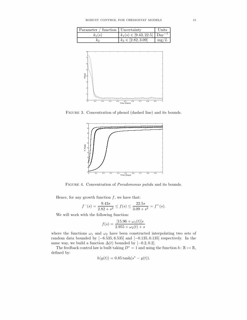
Figure 3. Concentration of phenol (dashed line) and its bounds.

0 0.1 0.2 0.3 0.4 0.5 0.6 0.7 0.8 0.9 10

1

2

3

4

5

6

7

8

9

10

Time (Days)

P. P

utid

a

Figure 4. Concentration of Pseudomonas putida and its bounds.

Hence, for any growth function f , we have that:

f−(s) =9.43s

2.82 + s2≤ f(s) ≤

22.5s

3.09 + s2= f+(s).

We will work with the following function:

f(s) =[15.96 + ω1(t)]s

2.955 + ω2(t) + s

where the functions ω1 and ω2 have been constructed interpolating two sets ofrandom data bounded by [−6.535, 6.535] and [−0.135, 0.135] respectively. In thesame way, we build a function ∆(t) bounded by [−0.2, 0.2].

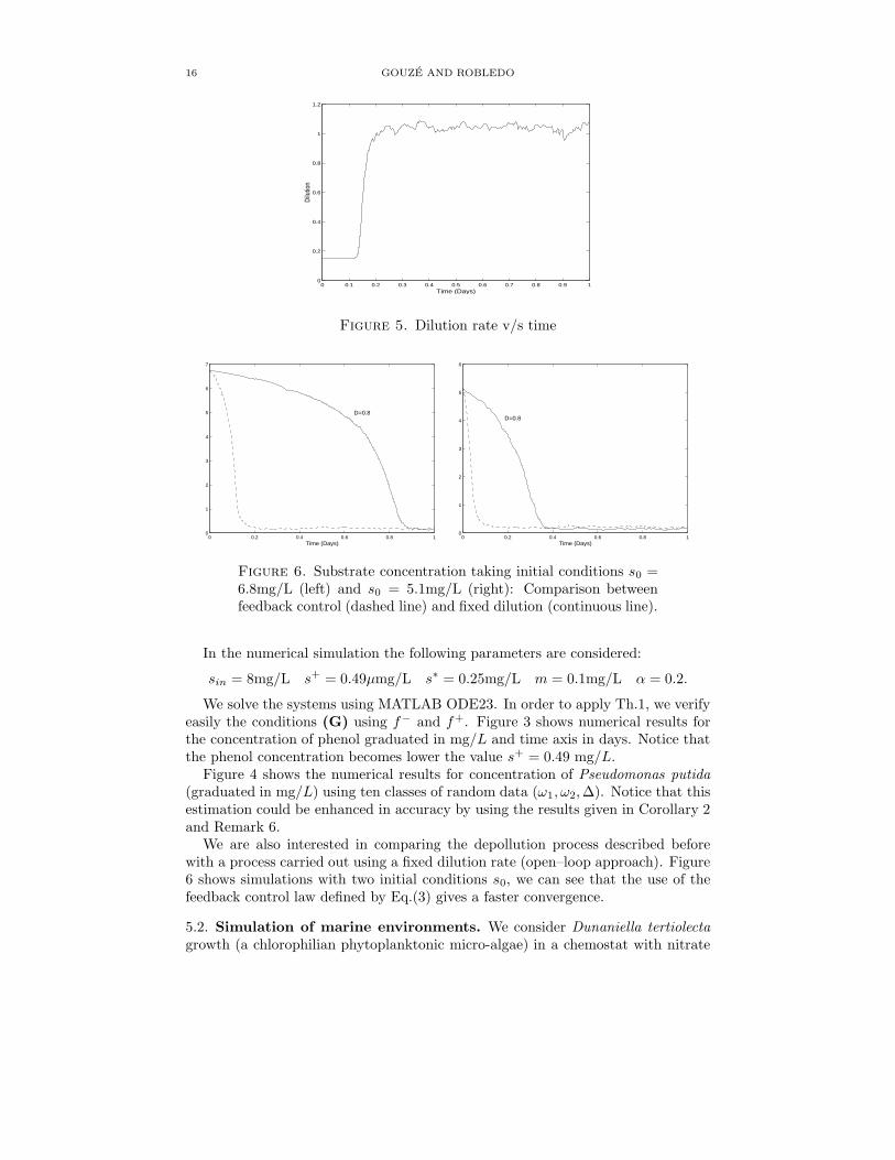
The feedback control law is built taking D∗ = 1 and using the function h : R 7→ R,defined by:

h(y(t)) = 0.85 tanh(s∗ − y(t)).


0 0.1 0.2 0.3 0.4 0.5 0.6 0.7 0.8 0.9 10

0.2

0.4

0.6

0.8

1

1.2

Time (Days)

Dilu

tion

Figure 5. Dilution rate v/s time

0 0.2 0.4 0.6 0.8 10

1

2

3

4

5

6

7

Time (Days)

D=0.8

0 0.2 0.4 0.6 0.8 10

1

2

3

4

5

6

Time (Days)

D=0.8

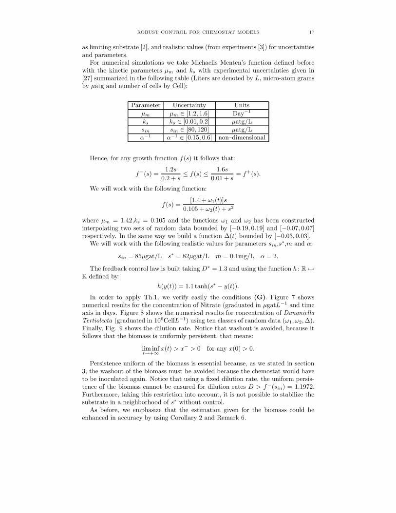
Figure 6. Substrate concentration taking initial conditions s0 =6.8mg/L (left) and s0 = 5.1mg/L (right): Comparison betweenfeedback control (dashed line) and fixed dilution (continuous line).

In the numerical simulation the following parameters are considered:

sin = 8mg/L s+ = 0.49µmg/L s∗ = 0.25mg/L m = 0.1mg/L α = 0.2.

We solve the systems using MATLAB ODE23. In order to apply Th.1, we verifyeasily the conditions (G) using f− and f+. Figure 3 shows numerical results forthe concentration of phenol graduated in mg/L and time axis in days. Notice thatthe phenol concentration becomes lower the value s+ = 0.49 mg/L.

Figure 4 shows the numerical results for concentration of Pseudomonas putida

(graduated in mg/L) using ten classes of random data (ω1, ω2, ∆). Notice that thisestimation could be enhanced in accuracy by using the results given in Corollary 2and Remark 6.

We are also interested in comparing the depollution process described beforewith a process carried out using a fixed dilution rate (open–loop approach). Figure6 shows simulations with two initial conditions s0, we can see that the use of thefeedback control law defined by Eq.(3) gives a faster convergence.

5.2. Simulation of marine environments. We consider Dunaniella tertiolecta

growth (a chlorophilian phytoplanktonic micro-algae) in a chemostat with nitrate


as limiting substrate [2], and realistic values (from experiments [3]) for uncertaintiesand parameters.

For numerical simulations we take Michaelis Menten’s function defined beforewith the kinetic parameters µm and ks with experimental uncertainties given in[27] summarized in the following table (Liters are denoted by L, micro-atom gramsby µatg and number of cells by Cell):

Parameter Uncertainty Units

µm µm ∈ [1.2, 1.6] Day−1

ks ks ∈ [0.01, 0.2] µatg/Lsin sin ∈ [80, 120] µatg/Lα−1 α−1 ∈ [0.15, 0.6] non–dimensional

Hence, for any growth function f(s) it follows that:

f−(s) =1.2s

0.2 + s≤ f(s) ≤

1.6s

0.01 + s= f+(s).

We will work with the following function:

f(s) =[1.4 + ω1(t)]s

0.105 + ω2(t) + s2

where µm = 1.42,ks = 0.105 and the functions ω1 and ω2 has been constructedinterpolating two sets of random data bounded by [−0.19, 0.19] and [−0.07, 0.07]respectively. In the same way we build a function ∆(t) bounded by [−0.03, 0.03].

We will work with the following realistic values for parameters sin,s∗,m and α:

sin = 85µgat/L s∗ = 82µgat/L m = 0.1mg/L α = 2.

The feedback control law is built taking D∗ = 1.3 and using the function h : R 7→R defined by:

h(y(t)) = 1.1 tanh(s∗ − y(t)).

In order to apply Th.1, we verify easily the conditions (G). Figure 7 showsnumerical results for the concentration of Nitrate (graduated in µgatL−1 and timeaxis in days. Figure 8 shows the numerical results for concentration of Dunaniella

Tertiolecta (graduated in 106CellL−1) using ten classes of random data (ω1, ω2, ∆).Finally, Fig. 9 shows the dilution rate. Notice that washout is avoided, because itfollows that the biomass is uniformly persistent, that means:

lim inft→+∞

x(t) > x− > 0 for any x(0) > 0.

Persistence uniform of the biomass is essential because, as we stated in section3, the washout of the biomass must be avoided because the chemostat would haveto be inoculated again. Notice that using a fixed dilution rate, the uniform persis-tence of the biomass cannot be ensured for dilution rates D > f−(sin) = 1.1972.Furthermore, taking this restriction into account, it is not possible to stabilize thesubstrate in a neighborhood of s∗ without control.

As before, we emphasize that the estimation given for the biomass could beenhanced in accuracy by using Corollary 2 and Remark 6.


0 2 4 6 8 10 12 14 16 18 2064

66

68

70

72

74

76

78

80

82

84

Time (Days)

Nitr

ate

Figure 7. Concentration of nitrate (dashed line) and its bounds.

0 2 4 6 8 10 12 14 16 18 200

0.5

1

1.5

2

2.5

3

Time (Days)

Dun

anie

lla

Figure 8. Concentration of Dunaniella tertiolecta and its bounds.

0 2 4 6 8 10 12 14 16 18 200

0.5

1

1.5

2

2.5

Time (Days)

Dilu

tion

Figure 9. Dilution rate v/s time

6. Discussion

The problem (P) of feedback stabilization for a chemostat with uncertainties onits outputs and internal structure has been discussed. It has been shown that, givenknown bounds for the uncertainties and some technical assumptions, we are able to


build a family of feedback control laws, which stabilize the system in a bounded set.Our approach is based on the theory of monotone dynamical systems. Furthermore,we do not assume that the uncertainties satisfy some dynamical and/or statisticalproperties, excluding by consequence the use of some robust control approachesgiven by [4] and [15].

It must be noted that, contrarily to the bibliography stated in introduction, wehave considered models with mortality rate m > 0, that makes the problem farmore difficult because the “conservation principle” is not verified.

Many extensions are available in the spirit of (H1) and/or (H2): for exampleto suppose that the parameter sin is unknown and verifies s−in(t) ≤ sin ≤ s+

in(t) forany t ≥ 0 and the functions s−in,s+

in are bounded and measurable.Another natural extension of the present work would be to treat outputs of

type y(t) = s(t) + ∆(t) (additive disturbance). These two extensions can be cer-tainly solved by the methods presented in the proof of Th.1 combined with alter-native/additional hypothesis.

There are some problems related but are far beyond the framework of this pa-per: in Remark 5 we show how a feedback control law can improve the speed ofconvergence toward a critical point. It will desirable to study global results andtheir robustness. Other related problems concern the case of competition in thechemostat, delays in some input variables (time necessary to measure the output)and state variables (delay between changes in the substrate concentration and thecorresponding changes in the microorganisms).

Concluding the discussion of the control of an uncertain chemostat, we recall thatother formulations are known. For example, a stabilization problem for an uncertainmodel of dynamics of carbon in the atmosphere is developed by Kryazhimiskyand Maksimov in [16]. Inspired by game-theoretical control problems, the authorsstabilize the amount of carbon in the atmosphere. It would be extremely interestingto examine this approach in our future work.

Acknowledgments: The authors would like to thank O. Bernard and L. Mailleret(INRIA–Projet COMORE) for valuable discussions. This research has been suppor-ted in part by the science and technology council of Chile (CONICYT) in the frameof INRIA–CONICYT cooperation agreement.

Appendix: Planar cooperative systemsIn this appendix we present some definitions and results from the theory of planar

cooperative systems [22],[23].

Definition 1. A vector field in the Euclidean space determines a cooperative system

of differential equations provided that all the off–diagonal terms of its Jacobianmatrix are nonnegative on a convex domain of R

n.

Let us define an order in R2 by ~y ≤ ~x if ~x− ~y ∈ R

2+, i.e. yi ≤ xi for any i = 1, 2.

The goal is to study the asymptotic behavior of the cooperative system:

(18) x = F (x)

and to compare its solutions with these ones of the following systems:

(19) z = G(z),

(20) y = H(y)

provided that the continuous functions G,H : Ω 7→ R2 verify H ≤ F ≤ G.


Proposition 1 (Comparison Theorem). Assume that system (18) is cooperative.

Moreover, let x(t) be a solution of (18) defined on [a, b], hence:

(i) If z(t) is a continuous function on [a, b] satisfying (19) on (a, b) with z(a) ≤x(a), then z(t) ≤ x(t) for all t in [a, b].

(ii) If y(t) is a continuous function on [a, b] satisfying (20) on (a, b) with y(a) ≥x(a), then y(t) ≥ x(t) for all t in [a, b].

Proof. See Theorem 3.5.1 from [23].

Proposition 2 (Asymptotic behavior). Assume that system (18) is cooperative.

Moreover, if, for any initial condition x0, ω(x0) has a compact closure, then the

solutions of system (18) are convergent to a critical point.

Proof. See Theorem 3.2.2 from [23].

References

[1] Bastin G, Dochain D. On–line estimation and adaptive control of bioreactors, Elsevier: Am-sterdam, 1990.

[2] Bernard O. Etude experimentale et theorique de la croissance de Dunaniella Tertiolecta

soumise a une limitation variable de nitrate, utilisation de la dynamique transitoire pour la

conception et la validation de modeles; PhD Thesis, Universite Paris VI, 1995.[3] Bernard O, Malara G, Sciandra A. The effects of a controlled fluctuating nutrient environment

on continuous cultures of phytoplankton monitored by computers; J.Exp.Mar.Biol.Ecol. 1996,197:263–278.

[4] Byrnes CI, Delli Priscoli F, Isidori A. Output regulation of uncertain nonlinear systems,Birkhauser: Boston, 1997

[5] Coddington E, Levinson N. Theory of ordinary differential equations, McGraw–Hill, 1955.[6] Dochain D. (Ed.) Automatique des bioprocedes. Hermes: Paris, 2001.[7] Gouze JL, Rapaport A, Hadj–Sadok MZ. Interval observers for uncertain biological systems.

Ecological Modelling. 2000, 133:45–56.[8] Hadj–Sadok MZ, Gouze JL. Estimation of uncertain models of activated sludge processes

with interval observers. J.Proc.Contr. 2001, 11:299–310.[9] Henson MA, Seborg DE (Eds.) Nonlinear process control. Prentice Hall, 1997.

[10] Hofbauer J. A unified approach to persistence. Acta.Appl.Math. 1989, 14:11–22.[11] Hofbauer J, Sigmund K. Evolutionary games and population dynamics. Cambridge University

Press: Cambridge, 1998.[12] Keesman KJ, Stitger JD. Optimal parametric sensitivity control for the estimation of kinetic

parameters in bioreactors. Math.Biosc. 2002, 179:95–111.[13] Kieffer N, Walter E. Guaranteed parameter estimations for cooperative models. In Benvenuti

L, De Santis A, Farina L (Eds.), Positive systems, Lecture Notes in control and informationsciences, 294, Springer, 2003.

[14] Krasovskii NN, Subbotin AI. Game–Theoretical control problems. Springer–Verlag: New–York, 1988.

[15] Krstic M, Deng H. Stabilization of nonlinear uncertain systems. Springer–Verlag: London1998.

[16] Kryazhiminsky A, Maksimov V. On the exact stabilization of an uncertain dynamics. IIASA.Interim Report 03–067, 2003.

[17] Perruquetti W, Richard JP. Connecting Wasewski’s conditions with M–matrices: Applicationto constrained stabilization. Dynamic systems and Applications. 1996,5:81–96.

[18] Raisch J, Bruce F. Modeling deterministic uncertainty. In Levine W. (Ed.), The control

handbook, CRC Press, IEEE Press, 1996.[19] Rapaport A, Dochain D. Interval observers for biochemical processes with uncertain kinetics

and inputs. Math.Biosc. 2005, 193:235–253.

[20] Rapaport A, Harmand J. Robust regulation of a class of partially observed nonlinear contin-uous bioreactors. J.Proc.Contr. 2002, 12:291–302.

[21] Sokol W, Howell JA. Kinetics of phenol oxidation by washed cells. Biotech.Bioeng. 1981,23:2039–2049.


[22] Smith H, Waltman P. The theory of the chemostat. Dynamics of microbial competition.Cambridge Studies in Mathematical Biology, 13, Cambridge Univ. Press: Cambridge, 1995.

[23] Smith H. Monotone dynamical systems: an introduction to the theory of competitive and

cooperative systems. Mathematical surveys and monographs, 41, AMS: Providence, 1995.[24] Smith RJ, Wolkowicz GSK. Growth and competition in the nutrient driven self–cycling fer-

mentation process. Canadian Appl.Math.Quart. 2003; 10:171–177.[25] Thieme H. Convergence results and a Poincare–Bendixson trichotomy for asymptotically

autonomous differential equations. J.Math.Biol. 1992, 30:755–763.[26] Thieme H. Asymptotically autonomous differential equations in the plane.

Rock.Mount.Journ.Math. 1994, 24:351–380.[27] Vatcheva I, Bernard O, De Jong H, Mars N. Experiment Selection for the Discrimination of

Semi–Quantitative Models of Dynamical Systems. To appear in Artificial Intelligence.

E-mail address: gouze,[email protected]

INRIA Projet COMORE, 2004 Route des Lucioles, BP 93 06902 Sophia Antipolis(Cedex) France

Documents

ROBUST CONTROL FOR AN UNCERTAIN CHEMOSTAT MODEL … · ROBUST CONTROL FOR AN UNCERTAIN CHEMOSTAT MODEL JEAN{LUC GOUZE AND GONZALO ROBLEDO Abstract. In this paper we consider a control