Robotics: Science and Systems 2010Zaragoza, Spain June 27-30, 2010

1

A Fast Traversal Heuristic and Optimal Algorithmfor Effective Environmental Coverage

Ling Xu and Tony StentzRobotics Institute, Carnegie Mellon University, Pittsburgh, PA, USA

{lingx, axs}@cs.cmu.edu

Abstract—Tasks such as street mapping and security surveil-lance seek a route that traverses a given space to perform afunction. These task functions may involve mapping the spacefor accurate modeling, sensing the space for unusual activity,or processing the space for object detection. With a prior map,an optimal path can be computed using a graph to representthe environment and generating the solution using known graphalgorithms. However, the prior map may be inaccurate due tofactors such as occlusion, outdatedness, dynamic objects, andresolution limitations. In this work, we address the NP-hardproblem of optimal environmental coverage with incompleteprior map information.To utilize related algorithms in graph theory, we represent the

environment as a graph. Using this representation, we present agraph coverage approach for optimal plan generation based onthe Undirected Chinese Postman and Rural Postman problems.This approach produces a tractable solution through the use oflow complexity algorithms in a branch-and-bound framework.Additionally, as the robot receives sensor updates during traversalof the environment, we update the graph to reflect those changes.The updated graph can be highly disconnected so computing anoptimal solution can be NP-hard. To combat this, we introducea heuristic for coverage path generation that helps maximize theconnectivity of the updated graph. We evaluate our approach ona set of comparison tests in simulation.

I. INTRODUCTIONMany tasks, such as street sweeping, mail delivery, and

robotic surveillance and patrol, require a robot to visit allpoints in an environment to accomplish a goal. These goalsusually entail effectively mapping, sensing, or processing thespace. In this work, we address this coverage problem wherea robot is required to visit most locations in a given area.We assume a map of the environment is available. This isa reasonable assumption since information of most outdoorspaces can be obtained via satellite images. However priormaps can differ from the actual environment due to factorssuch as occlusions, datedness, and lower map resolutions.Even with an otherwise accurate map, dynamic conditionssuch as the presence of people or vehicles can diminishthe effective accuracy of prior information. Therefore, anadditional goal for the coverage problem we are addressing isto efficiently replan when changes occur in the environment.In robotics, there is a number of related work in the area

of continuous space coverage. In continuous space coverage,the robot must pass a detector over all points in the spacein order to complete a task [1][2][3][4]. While these methodsensure completeness in terms of the area covered, they do notguarantee optimal path length. In graph theory and operations

research, researchers have tackled this problem by representingthe environment as a graph, and using routing algorithms suchas the traveling salesman [5] [6] or postman problems [7] [8] togenerate optimal solutions. Because we seek optimal paths forcoverage efficiency, we choose to use the graph representationas the foundation of our solution approach.In the graph representation, nodes in the graph denote

locations in the environment and edges in the graph are thepaths between the locations. For example, the map in Figure1 is converted into a graph shown in Figure 2(a) by changingeach street intersection into a node and each street into anedge. Each edge has a cost assigned to it where the cost canrepresent measurements such as Euclidean distance betweenlocations, terrain traversability, travel time, or a combination ofseveral metrics. Additionally, each edge is undirected meaningit can be traversed in both directions. Another example is aVoronoi diagram where the paths are edges in the graph andthe path intersections are nodes. This is one way to generateoptimal paths for some of the problems in continuous spacecoverage.For our problem, we seek a coverage path that visits all the

edges or a designated edge subset of the graph. This coverageproblem can be modeled as an arc-routing problem. We focuson two types of arc-routing problems: the Chinese PostmanProblem [9] and the Rural Postman Problem. The ChinesePostman Problem (CPP) seeks an optimal path that visits allthe edges of the graph at least once, and the Rural PostmanProblem (RPP) seeks an optimal path that visits a predefinedsubset of graph edges at least once. We define an optimalpath as the lowest cost coverage path given the current graphinformation.The CPP and RPP differ in two ways. The CPP has a

polynomial time solution of O(n3) [7] [10]. It works wellfor applications where it is necessary to traverse every part ofthe space. For example, Sorensen uses the CPP to plan toursfor farming machines in static known environments [11].In many practical problems, it is not necessary to traverse

all the edges in the graph. The RPP seeks a tour that traversesa required subset of the graph edges using the extra graphedges as travel links between the required edges. Unlike theCPP, the RPP is a NP-hard problem. Optimal solutions existthat formulate the RPP as an integer linear program andsolve it using branch-and-bound [8]. One recent approach [12]introduced new dominance relations such as computing theminimum spanning tree on the connected components in a

Fig. 1. The map of an urban environment is shown where the box-like shapesrepresent buildings and the spaces between the buildings are roads.

graph to solve large problem instances. Additionally, manyTSP heuristics have been extended to the RPP [13]. Forexample, Christofides’ approximation for the Euclidean TSPwas modified for the undirected RPP and maintains its 3

2

constant factor performance [14]. Improvements heuristicshave been developed as postoptimality procedures for theseapproximation algorithms by modifying and shortening thesuboptimal solution path to be as close to optimal as pos-sible [15].While most research on arc routing problems focus on the

static environments, there has been work that address dynamicgraphs. Moreira et al. present a heuristic-based approach forthe Dynamic Rural Postman Problem (DRPP) [16]. Theyframe the problem as a machine cutting application wherethe graph changes as pieces of the cutting surface are cutand removed. They introduce and compare two heuristics forchoosing the next edge to cut. While the run times theyobtained were reasonable, the solution paths generated werenot optimal.In this paper, we present two contributions. First, we in-

troduce a general approach for the online coverage problemwith an incomplete prior map. As changes in the environmentare detected, we present a method for updating the graphto reflect the new changes. Our approach uses the lowercomplexity Chinese Postman algorithm within a branch-and-bound framework to solve the harder Rural Postman problem.Second, we present a new heuristic for path generation thattraverses the graph in such a way that when changes occur, theheuristic helps keep the new coverage problem polynomial.The rest of the paper is organized as follows. In Section II,

we introduce and describe each component of the coveragealgorithm. In the next section, we explain the set of tests weconducted. The results are presented and discussed in SectionIV. Finally, we conclude and list future directions for this work.

II. COVERAGE ALGORITHM

A. Chinese Postman ProblemWe assume the environment is initially known in the form

of a prior map. This prior map is converted into a graphstructure with goal locations as nodes in the graph and pathsbetween goals as edges in the graph. The first step in solvingthe coverage problem is to assume the prior map is accurateand generate a tour that covers all the edges in the graph. Thisproblem can be represented as a Chinese Postman Problem(CPP).

(a)

(b)

Fig. 2. (a) We represent the prior map as a graph where edges (white lines)denote the roads and vertices (stars) denote the road intersections. (b) Dottedand solid lines represent the CPP solution and are super-imposed on the abovegraph. Dotted lines denote edges that are traversed once and solid lines denoteedges that are traversed more than once.

Algorithm 1: Chinese Postman Problem AlgorithmInput: s, start vertex

G, connected graph where each edge has a cost valueOutput: P , tour found or empty if no tour foundif IsEven(G) then1

P = FindEulerCycle(G, s);2else3

O = FindOddV ertices(G);4O! = FindAllPairsShortestPath(O);5Mate = FindMinMatching(O!);6G! = (G,Mate);7P = FindEulerCycle(G!, s);8

end9return P ;10

The CPP optimal tour consists of traversing all the edgesin the graph at least once and starting and ending at thesame node. To solve this problem, we used the Edmonds andJohnson algorithm [17] [18], detailed in Algorithm 1.The first step in the algorithm is to calculate the degree

of each vertex. If all the vertices have even degree, then thealgorithm finds an Euler tour using the End-Pairing technique(line 2). If any vertices have odd degree, a minimum weightedmatching [19][20] among the odd degree vertices is foundusing an all pairs shortest path graph of the odd vertices (line5). Because the matching algorithm requires a complete graph,the all pairs shortest pairs algorithm is a way to optimallyconnect all the odd vertices. The matching finds the minimumcost set of edges that connect the odd nodes (line 6). Theedges in the matching are doubled in the graph making thedegree of the odd nodes even (line 7). Finally, the algorithmfinds a tour on the new Eulerian graph (line 8).We ran the CPP algorithm on the example graph shown

earlier. Since the graph is odd, a solution to the problemrequires some of the edges to be traversed more than once.In Figure 2(b), the solution tour is depicted where the dottedand solid lines represent edges traversed once and edgestraversed more than once, respectively.

B. Rural Postman ProblemIn the Rural Postman Problem, there are two sets of graph

edges: required and optional. We define the required subsetof edge as coverage edges, and the optional subset as traveledges. Any solution would include all coverage edges andsome combination of travel edges.For combinatorial optimization problems such as the RPP,

a common planning framework is branch-and-bound [21].Branch-and-bound is a method of iterating through a set ofsolutions until an optimal solution is found. It consists of twosteps, a branching step and a bounding step. In the branchingstep, the algorithm forms n branches of subproblems whereeach subproblem is a node in the branch-and-bound tree. Thesolution to any subproblem could lead to a solution to theoriginal problem. In the bounding step, the algorithm computesa lower bound for the subproblem. These lower bounds enablebranch-and-bound to guarantee a solution is optimal withouthaving to search through all possible subproblems. Branch-and-bound is a general method for handling hard problemsthat are slight deviations from low complexity problems eventhough faster, ad hoc algorithms exist for each deviation. Theprocess of partitioning the problem into subproblems worksto our advantage since it enables the use of the applicationsof low complexity algorithms like the CPP as bounds on thesubproblems.In our approach, we use the branch-and-bound approach to

iterate through all combinations of travel edges. We call theset of travel edges our partition set. At each branching step,we generate two subproblems by including and excluding atravel edge. Next, each subproblem in the branch-and-boundtree is solved using the CPP algorithm. The cost of the CPPsolution is the lower bound on the cost of the RPP for theparticular branch. If the travel set is large, this method can becomputationally expensive.To keep computation costs low, we reduce the partition set

given to the branch and bound algorithm. First, we define afew terms used in the algorithm. A coverage or travel vertexis a vertex in the graph incident to only coverage or traveledges, respectively. A border vertex is a vertex in the graphincident to at least one coverage edge and at least one traveledge. A travel path is a a sequence of travel segments andtravel vertices connecting a pair of border vertices. Finally,an optimal travel path (OTP) is a travel path connecting apair of border vertices such that it is the lowest cost path (ofany type) between the vertices, and the vertices are not in thesame cluster (i.e., there is no path consisting of just coveragesegments between them). In other words, OTPs are shortestpaths between clusters of coverage segments that do not cutthrough any part of a coverage cluster. Additionally, we modifythe CPP algorithm to permit the use of travel edges as part ofthe shortest path between the set of odd nodes. This allowsthe CPP to reason directly about the paths that cut throughcoverage clusters.All the OTPs are computed by finding the lowest cost path

pij (searching over the entire graph) between each pair ofborder vertices vi and vj in different clusters. If pij is a travel

path, we save it as an OTP. If pij is not a travel path, then viand vj do not have an OTP between them (i.e., pij = NULL).The OTPs become our partition set. The OTPs are unlabeled atthe beginning of the algorithm. We iterate through the OTP setwithin the branch-and-bound framework. At each branch step,the algorithm generates a new subproblem by either includingor excluding an OTP. At the beginning of the RPP algorithmshown in Algorithm 2, we assign cost 0 to the unlabeled OTPsand solve the problem with all the OTPs set as required edgesusing the CPP algorithm (lines 2,3). The problem and CPP costare pushed onto a priority queue (line 4). The CPP cost is thelower bound on the problem since all the OTPs have zero cost.While the queue is not empty, the lowest cost subproblem isselected from the queue (lines 5,6).

Algorithm 2: Rural Postman Problem AlgorithmInput: s, start vertex

G = (C, T ), graph where each edge has a label and acost value. C is the subset of coverage edges, and T isthe subset of travel edgesOTP , subset of OTPs

Output: P , tour found or empty if no tour foundpq = [];1G! = [G,OTP ] where !OTP , cost(pij) = 02P = CPP (s,G!);3AddToPQ(pq, [G!, P ]);4while !isEmpty(pq) do5

[G!, P ] = PopLowestCost(pq);6pij = FindMaxOTP (G!);7if pij == [] then8

return P ;9end10G!! = IncludeEdge(G!, pij);11P1 = CPP (s,G!!);12AddToPQ(pq, [G!!, P1]);13G!! = RemoveEdge(G!, pij);14P2 = CPP (s,G!!);15AddToPQ(pq, [G!!, P2]);16

end17return []18

For the subproblem, the algorithm selects an unlabeled OTPpij with the highest path cost (line 7). By employing thisstrategy of choosing the OTP with the highest path cost, ouraim is to increase the lower bound by the largest amount,which may help focus the search to the correct branch andprevent extraneous explorations. Once an OTP pij is selected,two branches are generated; the first branch includes pij in thesolution (line 11), this time with the real path cost assigned,and the second branch omits pij from the solution (line 14). Asolution to each branch is found using the CPP algorithm (lines12,15). Because each solutions is generated with a cost of 0assigned to the unlabeled OTPs in the subproblem, the costsof the inclusion and exclusion CPP solutions represent lowerbounds on the cost of the RPP with and without using pij fortravel, respectively. These new subproblems are added to thepriority queue (lines 13, 16), and the algorithm iterates untilthe lowest cost problem in the queue contains no OTPs (line8). The solution to this problem is the optimal solution to theRPP since it has either included or excluded every single OTP

in the solution, and has a path cost that is equal to or lowerthan the lower bounds of the other branches. The branch-and-bound algorithm for the RPP is an exponential algorithm witha complexity of O(|V |32t) where t is the number of OTPs and|V | is the number of vertices in the graph.

C. Online ChangesDynamic changes occur when the environment differs from

the original map. There are two categories of planners thathandle these differences. Contingency planners model the un-certainty in the environment and plan for all possible scenarios.Assumptive planners [22] presume the perceived world stateis correct and plan based on this assumption. If disparitiesarise, the perceived state is corrected and replanning occurs.We choose to use the lower complexity assumptive planningin order to generate solutions quickly.In our planner, an initial plan is found based on the graph of

the environment. As the vehicle uncovers differences betweenthe map and environment during traversal, the algorithm prop-agates them into the graph structure. This may require a simplegraph modification such as adding, removing, or changing thecost of an edge. But it can also result in more significant graphrestructuring. As mentioned earlier, these changes may convertthe initial planning problem into an entirely different problem.For the coverage problems we are addressing in this work,

most changes to the environment are discovered when therobot is actively traversing the space. These online changes aretypically detected when the robot is not at the starting location,but at a middle location along the coverage path. At this point,some of the edges have already been visited. Because it is notnecessary to revisit the edges that are already traversed, thevisited edges in the previous plan are converted to travel edges.As shown in Algorithm 3, if the unvisited edges in the newproblem are connected, we run the CPP algorithm; otherwise,we run the RPP.When environmental changes are found online, replanning

is done on the updated graph with different starting and endingvertices. To remedy this disparity, we add an artificial edgefrom the current vehicle location c to the ending vertex s inthe graph (line 3). This edge (c, s) is assigned a large costvalue to prevent it from being doubled in the solution. Usingthis modified graph, a tour from s to s is found. The edge(c, s) is then deleted from the graph and from the tour (line11). The algorithm adjusts the coverage path to start at thecurrent location and travel to the end location (line 12). Thetable below shows the details for adjusting the path. The termson the left hand side indicates the four possible initial pathconfigurations where s!c indicates an edge. The terms inthe middle are the procedures for adjusting the specific path,and the terms on the right are the final paths returned by thecoverage algorithm.

s...s!(c...s) " (c...s)!s...s " c...s...s(s...c)!s...s " Reverse(s...c)!s...s " c...s...ss!(c...s) " (c...s)!s " c...s(s...c)!s " Reverse(s...c)!s " c...s

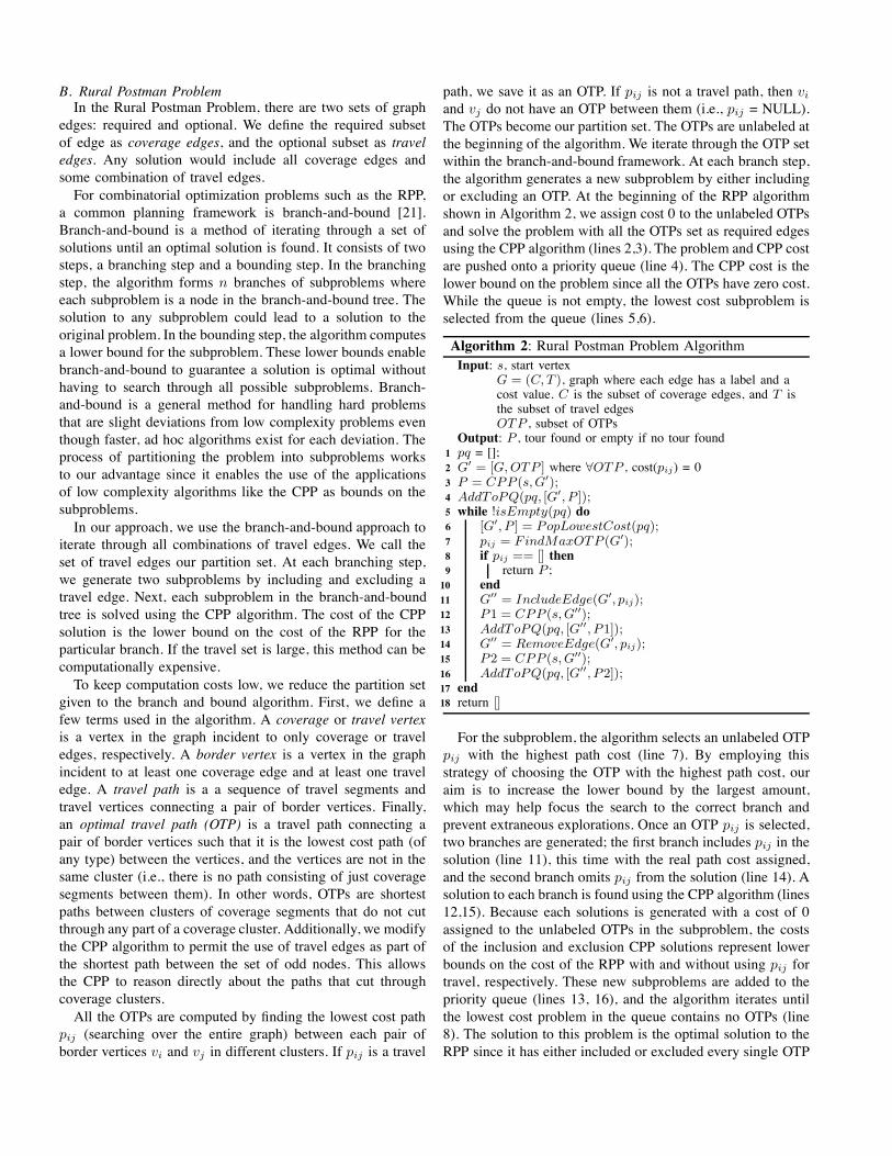
Fig. 3. During traversal of the CPP solution, the robot discovers that thethird edge in the path is missing and ends the traversal. Dotted lines denoteedges that are traversed once and solid lines denote edges that are traversedmore than once.

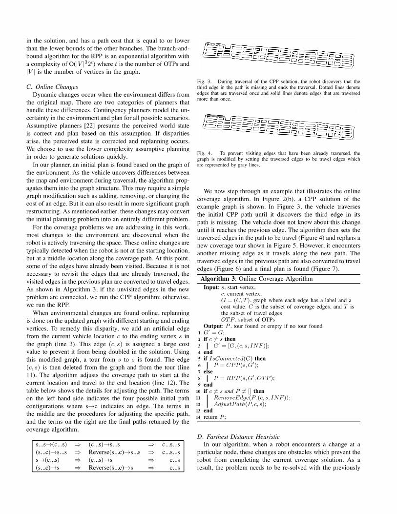
Fig. 4. To prevent visiting edges that have been already traversed, thegraph is modified by setting the traversed edges to be travel edges whichare represented by gray lines.

We now step through an example that illustrates the onlinecoverage algorithm. In Figure 2(b), a CPP solution of theexample graph is shown. In Figure 3, the vehicle traversesthe initial CPP path until it discovers the third edge in itspath is missing. The vehicle does not know about this changeuntil it reaches the previous edge. The algorithm then sets thetraversed edges in the path to be travel (Figure 4) and replans anew coverage tour shown in Figure 5. However, it encountersanother missing edge as it travels along the new path. Thetraversed edges in the previous path are also converted to traveledges (Figure 6) and a final plan is found (Figure 7).Algorithm 3: Online Coverage AlgorithmInput: s, start vertex,

c, current vertex,G = (C, T ), graph where each edge has a label and acost value. C is the subset of coverage edges, and T isthe subset of travel edgesOTP , subset of OTPs

Output: P , tour found or empty if no tour foundG! = G;1if c "= s then2

G! = [G, (c, s, INF )];3end4if IsConnected(C) then5

P = CPP (s,G!);6else7

P = RPP (s,G!, OTP );8end9if c "= s and P "= [] then10

RemoveEdge(P, (c, s, INF ));11AdjustPath(P, c, s);12

end13return P ;14

D. Farthest Distance HeuristicIn our algorithm, when a robot encounters a change at a

particular node, these changes are obstacles which prevent therobot from completing the current coverage solution. As aresult, the problem needs to be re-solved with the previously

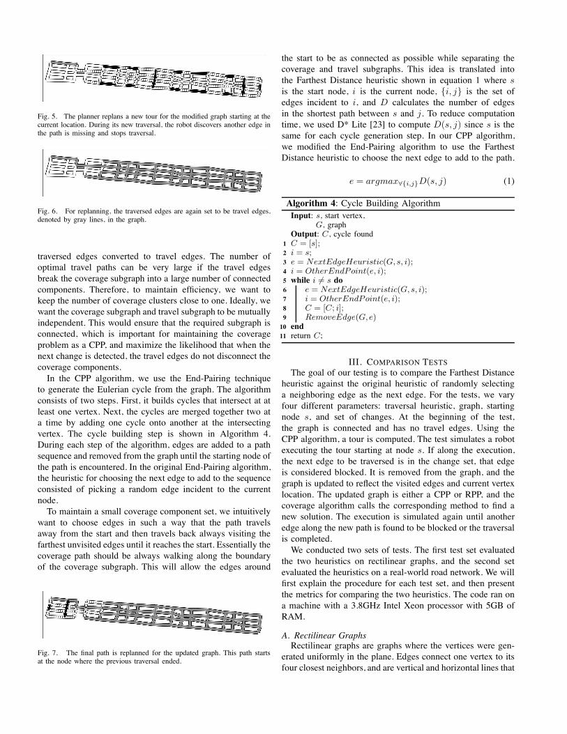
Fig. 5. The planner replans a new tour for the modified graph starting at thecurrent location. During its new traversal, the robot discovers another edge inthe path is missing and stops traversal.

Fig. 6. For replanning, the traversed edges are again set to be travel edges,denoted by gray lines, in the graph.

traversed edges converted to travel edges. The number ofoptimal travel paths can be very large if the travel edgesbreak the coverage subgraph into a large number of connectedcomponents. Therefore, to maintain efficiency, we want tokeep the number of coverage clusters close to one. Ideally, wewant the coverage subgraph and travel subgraph to be mutuallyindependent. This would ensure that the required subgraph isconnected, which is important for maintaining the coverageproblem as a CPP, and maximize the likelihood that when thenext change is detected, the travel edges do not disconnect thecoverage components.In the CPP algorithm, we use the End-Pairing technique

to generate the Eulerian cycle from the graph. The algorithmconsists of two steps. First, it builds cycles that intersect at atleast one vertex. Next, the cycles are merged together two ata time by adding one cycle onto another at the intersectingvertex. The cycle building step is shown in Algorithm 4.During each step of the algorithm, edges are added to a pathsequence and removed from the graph until the starting node ofthe path is encountered. In the original End-Pairing algorithm,the heuristic for choosing the next edge to add to the sequenceconsisted of picking a random edge incident to the currentnode.To maintain a small coverage component set, we intuitively

want to choose edges in such a way that the path travelsaway from the start and then travels back always visiting thefarthest unvisited edges until it reaches the start. Essentially thecoverage path should be always walking along the boundaryof the coverage subgraph. This will allow the edges around

Fig. 7. The final path is replanned for the updated graph. This path startsat the node where the previous traversal ended.

the start to be as connected as possible while separating thecoverage and travel subgraphs. This idea is translated intothe Farthest Distance heuristic shown in equation 1 where sis the start node, i is the current node, {i, j} is the set ofedges incident to i, and D calculates the number of edgesin the shortest path between s and j. To reduce computationtime, we used D* Lite [23] to compute D(s, j) since s is thesame for each cycle generation step. In our CPP algorithm,we modified the End-Pairing algorithm to use the FarthestDistance heuristic to choose the next edge to add to the path.

e = argmax!{i,j}D(s, j) (1)

Algorithm 4: Cycle Building AlgorithmInput: s, start vertex,

G, graphOutput: C, cycle foundC = [s];1i = s;2e = NextEdgeHeuristic(G,s, i);3i = OtherEndPoint(e, i);4while i "= s do5

e = NextEdgeHeuristic(G,s, i);6i = OtherEndPoint(e, i);7C = [C; i];8RemoveEdge(G,e)9

end10return C;11

III. COMPARISON TESTSThe goal of our testing is to compare the Farthest Distance

heuristic against the original heuristic of randomly selectinga neighboring edge as the next edge. For the tests, we varyfour different parameters: traversal heuristic, graph, startingnode s, and set of changes. At the beginning of the test,the graph is connected and has no travel edges. Using theCPP algorithm, a tour is computed. The test simulates a robotexecuting the tour starting at node s. If along the execution,the next edge to be traversed is in the change set, that edgeis considered blocked. It is removed from the graph, and thegraph is updated to reflect the visited edges and current vertexlocation. The updated graph is either a CPP or RPP, and thecoverage algorithm calls the corresponding method to find anew solution. The execution is simulated again until anotheredge along the new path is found to be blocked or the traversalis completed.We conducted two sets of tests. The first test set evaluated

the two heuristics on rectilinear graphs, and the second setevaluated the heuristics on a real-world road network. We willfirst explain the procedure for each test set, and then presentthe metrics for comparing the two heuristics. The code ran ona machine with a 3.8GHz Intel Xeon processor with 5GB ofRAM.

A. Rectilinear GraphsRectilinear graphs are graphs where the vertices were gen-

erated uniformly in the plane. Edges connect one vertex to itsfour closest neighbors, and are vertical and horizontal lines that

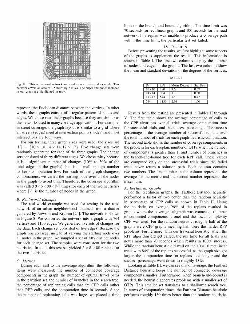
Fig. 8. This is the road network we used as our real-world example. Thisnetwork covers an area of 1.5 miles by 2 miles. The edges and nodes includedin our graph are highlighted in gray.

represent the Euclidean distance between the vertices. In otherwords, these graphs consist of a regular pattern of nodes andedges. We chose rectilinear graphs because they are similar tothe networks used in many coverage applications. For example,in street coverage, the graph layout is similar to a grid whereall streets (edges) meet at intersection points (nodes), and mostintersections are four ways.For our testing, three graph sizes were used; the sizes are

|V | = {10 # 10, 14 # 14, 17 # 17}. Five change sets wererandomly generated for each of the three graphs. The changesets consisted of thirty different edges. We chose thirty becauseit is a significant number of changes (10% to 30% of thetotal edges in the graphs), but is a small enough numberto keep computation low. For each of the graph-changesetcombinations, we varied the starting node over all the nodesin the graph to avoid bias. Therefore, the coverage algorithmwas called 3#5#30# |V | times for each of the two heuristicswhere |V | is the number of nodes in the graph.

B. Real-world ExampleThe real-world example we used for testing is the road

network of an urban neighborhood obtained from a datasetgathered by Newson and Krumm [24]. The network is shownin Figure 8. We converted the network into a graph with 764vertices and 1130 edges. We generated five sets of changes forthe data. Each change set consisted of five edges. Because thegraph was so large, instead of varying the starting node overall nodes in the graph, we sampled a set of fifty distinct nodesfor each change set. The samples were consistent for the twoheuristics. In total, this test set yielded 5# 5# 50 replans forthe two heuristics.

C. MetricsDuring each call to the coverage algorithm, the following

items were measured: the number of connected coveragecomponents in the graph, the number of optimal travel pathsin the partition set, the number of branches in the search tree,the percentage of replanning calls that are CPP calls ratherthan RPP calls, and the computation time in seconds. Sincethe number of replanning calls was large, we placed a time

limit on the branch-and-bound algorithm. The time limit was70 seconds for rectilinear graphs and 100 seconds for the roadnetwork. If a replan was unable to produce a coverage pathwithin the time limit, the particular test set failed.

IV. RESULTSBefore presenting the results, we first highlight some aspects

of the graphs to supplement the results. This information isshown in Table I. The first two columns display the numberof nodes and edges in the graphs. The last two columns showthe mean and standard deviation of the degrees of the vertices.

TABLE I

|V | |E| Mean Degree Std Dev10!10 180 3.6 0.5714!14 364 3.7 0.5017!17 544 3.8 0.47764 1130 2.96 1.00

Results from the testing are presented in Tables II throughV. The first table shows the average percentage of calls tothe CPP algorithm over all trials, average computation timefor successful trials, and the success percentage. The successpercentage is the average number of successful replans overthe total number of trials for each graph-heuristic combination.The second table shows the number of coverage components inthe problem for each replan, number of OTPs when the numberof components is greater than 1, and number of branches inthe branch-and-bound tree for each RPP call. These valuesare computed only on the successful trials since the failedtrials never return a solution path. Each column containstwo numbers. The first number in the column represents theaverage for the metric and the second number represents themaximum.A. Rectilinear GraphsFor the rectilinear graphs, the Farthest Distance heuristic

performed a factor of two better than the random heuristicin percentage of CPP calls as shown in Table II. Usingthe heuristic, on average 96% of the replans resulted ingraphs where the coverage subgraph was connected (numberof connected components is one) and the lower complexityCPP was used. For the random heuristic, roughly half of thegraphs were CPP graphs meaning half were the harder RPPproblems. Furthermore, with our traversal heuristic, when theRPP algorithm did get called, the run time for all trials wasnever more than 70 seconds which results in 100% success.While the random heuristic did well on the 10#10 rectilineartrials with 84% of the replans successful, as the graph size gotlarger, the computation time for replans took longer and thesuccess percentage went down to roughly 43%.Looking at Table III, we can see that on average, the Farthest

Distance heuristic keeps the number of connected coveragecomponents smaller. Furthermore, when branch-and-bound isneeded, the heuristic generates problems with a smaller set ofOTPs. This smaller set translates to a shallower search tree.In terms of computation times, the Farthest Distance heuristicperforms roughly 150 times better than the random heuristic.

B. Real-world ExampleFor the road network, the Farthest Distance heuristic per-

formed more than a factor of two better than the randomheuristic in maintaining connectivity among the coverageedges as shown in Table IV. When using the random heuristic,due to the high number of calls to the RPP algorithm, the runtime on the majority of the trials exceeded the time limit. Incontrast, the Farthest Distance heuristic had 98.4% successrate. Part of the reason for the drastic difference in successeswas due to the large size of the graph (this graph is more thantwice the size of the 17# 17 graph). This resulted in the RPPalgorithm needing more computation time. As shown in TableV, the number of connected components was similar for bothheuristics. For the branch-and-bound data, we can see that thenumber of OTPs for the Farthest Distance heuristic was halfthe number of OTPs for the random heuristic which led to asmaller search tree.

C. Evaluation of the Coverage AlgorithmSo far, we have shown comparison results regarding the

Farthest Distance heuristic and the random heuristic. Next, wewant to show some results of the coverage algorithm. Fromthe road network data, we calculated the ratio of the traveledges over the total number of edges in the graphs for all thetrials. The mean of the distribution was 0.44 with a standarddeviation of 0.28. This denotes the travel set ranged fromalmost zero to almost the entire graph. Next, we calculated

TABLE II

Computational results I for Rectilinear Graphs|V | Heuristic CPP Calls Time(s) Success Percentage

10"10 Random 46.67% 1.68 84.21%FarDist 92.19% 0.01 100.0%

14"14 Random 55.18% 3.02 51.08%FarDist 97.63% 0.02 100.0%

17"17 Random 59.59% 3.25 42.57%FarDist 98.66% 0.02 100.0%

TABLE III

Computational results II for Rectilinear Graph|V | Heuristic Components OTPs Branches

10"10 Random 2.11, 9.0 35.62, 153.2 352.45, 7823.8FarDist 1.08, 3.8 9.42, 38.8 15.86, 268.6

14"14 Random 1.67, 7.2 38.96, 204.4 276.03, 3773.6FarDist 1.03, 3.6 11.30, 36.6 24.42, 324.0

17"17 Random 1.52, 6.6 38.79, 244.2 182.52, 2135.2FarDist 1.01, 2.8 11.97, 30.4 18.66, 106.2

TABLE IV

Computational results I for Road Network graph|V | Heuristic CPP Calls Time(s) Success Percentage

764 Random 34.39% 12.63 30.40%FarDist 87.25% 1.14 98.40%

TABLE V

Computational results II for Road Network data|V | Heuristic Components OTPs Branches

764 Random 1.62, 4.0 23.59, 56.6 53.47, 326.4FarDist 1.14, 2.8 12.44, 40.0 18.65, 63.6

0 200 400 600 800 1000 12000

10

20

30

40

50

60

70

# of Travel Edges

# of

OTP

s

Fig. 9. This graph shows the cor-respondence between the numberof travel edges, along the x-axis,and the number of OTPs, along they-axis, for the road network data.

0 10 20 30 40 50 60 700

50

100

150

200

250

300

350

400

450

# of OTPs

# of

Bra

nche

s

Fig. 10. This figure shows therelationship between the OTP setsize, along the x-axis, and the num-ber of branches in the search tree,along the y-axis, for the road net-work data.

0 10 20 30 40 50 60 700

10

20

30

40

50

60

70

80

90

100

# of OTPs

Run

Tim

e (s

)

Fig. 11. This figure shows therelationship between the OTP setsize, along the x-axis, and the com-putation time (shown in seconds),along the y-axis for the road net-work data.

0 50 100 150 200 250 3000

10

20

30

40

50

60

70

# of OTPs

Run

Tim

e (s

)

Fig. 12. This figure shows therelationship between the OTP setsize, along the x-axis, and the com-putation time (shown in seconds),along the y-axis for the rectilineargraph data.

the size of the OTP sets that corresponded to each travel set(Figure 9). The ratio of the OTPs to travel edges has a meanof 0.08 with a standard deviation of 0.14. This indicates thatour coverage algorithm dramatically reduced the partition setgiven to the branch-and-bound algorithm through the use ofOTPs.Next, we show how the smaller partition set affected the

search tree and run time. From Figure 10, the maximumnumber of branches in the search tree was 435. Given that thelargest number of travel edges was 1085, if we had used thetravel edges as the partition set, the branch-and-bound problemcorresponding to the maximum set would need to solve atleast 1085 subproblems before finding the optimal solution.The smaller search tree translated into faster computation asevidenced in Figure 11. Similarly, the relationship betweenthe number of OTPs and run time for the rectilinear graphs isshown in Figure 12.

D. DiscussionThe results show that the Farthest Distance heuristic im-

proves the percentage of CPP calls by a factor of two. Thedifference in the percentage between the rectilinear graphsand the road network is due to the lower degree of thevertices in the road network. As we can see from Figure 8,the road network is not a completely regular grid. There areintersections where more than four roads meet. Additionally,there are streets that dead end in one direction. One aspect ofthe graph that the heuristic relies on is that there is a path fromthe start node to another node j in the graph, and a path from j

back to the start. This assumption depends on path redundancyin the graph which may not hold for all graphs. For example,in a graph that contains bridges, the coverage problem willalmost definitely become the more complex RPP when graphchanges occur. This is due to the fact that converting a bridgeedge to a travel edge will usually separate the start nodeand the remaining unvisited edges into different components.Hence, covering a graph with multiple bridges will limit theperformance of not only the Farthest Distance heuristic, butalso the random heuristic.As shown in the results, the coverage algorithm greatly

reduces the size of the partition set used to search for asolution. By limiting the branch-and-bound algorithm to onlyreason about the travel edges that make up the optimal pathbetween boundary nodes, the faster CPP can be used toevaluate the remaining travel edges. For the RPP algorithm,the results show lower computation time on rectilinear graphsthan for the road network graph. This is due to the smallerproblem sizes of the rectilinear graphs. The larger problemsize not only increases the run time of the CPP algorithm, butit also increases the time it takes to generate the OTP set.

V. CONCLUSION AND FUTURE WORKWe present a general approach to the online coverage

problem with an incomplete prior map. By representing theenvironment as a graph, our algorithm leverages the lowercomplexity Chinese Postman algorithm to produce optimalcoverage solutions. This algorithm enables a faster run timeby reducing the partition set to sequences of edges ratherthan single edges. Our algorithm is highly efficient when thenumber of OTP edges is small compared to the number oftravel edges since it can exploit the faster CPP algorithm.This means a better connected graph can greatly decrease thecomputation time of our general coverage algorithm.To improve the connectivity of the coverage graph when

changes occur, we introduce a heuristic for generating thecoverage path. Results from testing show that the Farthest Dis-tance heuristic performs much better than the random heuristicin keeping the problem polynomial. One of the benefits ofthe Farthest Distance heuristic is that it is independent ofour coverage algorithm. For example, it can be added to anycoverage approach, either optimal or approximate, as a wayto lower the complexity of the coverage problem when graphchanges occur online.For future work, we plan to test this method on a physical

robot with real-time sensor updates to gather practical resultsof our approach. We also plan to extend this approach todirected and mixed graphs. Finally, we intend to investigate thepotential of using the Farthest Distance heuristic on additionalarc-routing problems.

ACKNOWLEDGMENTThis work was sponsored by the U.S. Army Research

Laboratory, under contract Robotics Collaborative TechnologyAlliance (contract number DAAD19-01-2-0012). The views

and conclusions contained in this document are those of theauthors and should not be interpreted as representing theofficial policies, either expressed or implied, of the ArmyResearch Laboratory or the U.S. Government.

REFERENCES[1] Howie Choset. Coverage for robotics - a survey of recent results. Annals

of Mathematics and Artificial Intelligence, 31:113 – 126, 2001.[2] Ercan U. Acar, Howie Choset, Alfred A. Rizzi, Prasad N. Atkar,

and Douglas Hull. Morse decompositions for coverage tasks. TheInternational Journal of Robotics Research, 21(4):331–344, 2002.

[3] Howie Choset, Sean Walker, Kunnayut Eiamsa-Ard, and Joel Burdick.Sensor-Based Exploration: Incremental Construction of the HierarchicalGeneralized Voronoi Graph. The International Journal of RoboticsResearch, 19(2):126–148, 2000.

[4] E.U. Acar, H. Choset, and Ji Yeong Lee. Sensor-based coverage withextended range detectors. IEEE Transactions on Robotics, 22(1):189–198, Feb. 2006.

[5] S. Lin and B. W. Kernighan. An effective heuristic algorithm for thetraveling-salesman problem. Operations Research, 21(2):498–516, 1973.

[6] David S. Johnson and Lyle A. Mcgeoch. The traveling salesmanproblem: A case study. In Local Search in Combinatorial Optimization.Wiley and Sons, 1997.

[7] H. A. Eiselt, Michel Gendreau, and Gilbert Laporte. Arc routingproblems, part i: The chinese postman problem. Operations Research,43(2):231–242, 1995.

[8] H. A. Eiselt, Michel Gendreau, and Gilbert Laporte. Arc routingproblems, part ii: The rural postman problem. Operations Research,43(3):399–414, 1995.

[9] M Guan. Graphic programming using odd and even points. ChineseMathematics, 1:273–277, 1962.

[10] Christos H. Papadimitriou and Kenneth Steiglitz. Combinatorial Opti-mization : Algorithms and Complexity. Dover Publications, July 1998.

[11] C.G. Sorensen, T. Bak, and R.N. Jorgensen. Mission planner foragricultural robotics. Agricultural Engineering International, 2004.

[12] Gianpaolo Ghiana and Gilbert Laporte. A branch-and-bound algorithmfor the Undirected Rural Postman Problem. Mathematical Programming,87(3):467–481, 2000.

[13] Gilbert Laporte. Modeling and solving several classes of arc rout-ing problems as traveling salesman problems. Comput. Oper. Res.,24(11):1057–1061, 1997.

[14] G. N. Frederickson. Approximation algorithms for some routingproblems. Mathematical Programming, 40:225–246, 1979.

[15] Alain Hertz, Gilbert Laporte, and Pierrette Nanchen Hugo. Improvementprocedures for the undirected rural postman problem. INFORMS J. onComputing, 11(1):53–62, 1999.

[16] Luıs M. Moreira, Jose F. Oliveira, A. Miguel Gomes, and J. SoeiroFerreira. Heuristics for a dynamic rural postman problem. Comput.Oper. Res., 34(11):3281–3294, 2007.

[17] Jack Edmonds and Ellis Johnson. Matching, Euler tours, and the ChinesePostman. Mathematical Programming, 5(1):88–124, 1973.

[18] Edward. Minieka. Optimization algorithms for networks and graphs.M. Dekker, New York :, 1978.

[19] Harold Neil Gabow. Implementation of algorithms for maximummatching on nonbipartite graphs. PhD thesis, Stanford, CA, USA, 1974.

[20] E. Rothberg. Implementation of H. Gabow’s weighted matching algo-rithm (1992). ftp://dimacs.rutgers.edu/pub/netflow/matching/weighted/.

[21] E. L. Lawler and D. E. Wood. Branch-and-bound methods: A survey.Operations Research, 14(4):699–719, 1966.

[22] Illah Nourbakhsh and Michael Genesereth. Assumptive planning andexecution: a simple, working robot architecture. Autonomous RobotsJournal, 3(1):49–67, 1996.

[23] S. Koenig and M. Likhachev. Improved fast replanning for robotnavigation in unknown terrain. In Proceedings of the IEEE InternationalConference on Robotics and Automation, volume 1, pages 968–975,2002.

[24] Seattle road network data. http://research.microsoft.com/en-us/um/people/jckrumm/MapMatchingData/data.htm.