Robot Arm Transformations, Path Planning, and Trajectories!

Robert Stengel! Robotics and Intelligent Systems !

MAE 345, Princeton University, 2017•! Forward and inverse kinematics•! Path planning

–! Voronoi diagrams and Delaunay triangulation–! Probabilistic Road Map–! Rapidly Exploring Random Tree

•! Closed-form trajectories; connecting the dots–! Polynomials and splines–! Acceleration profiles

Copyright 2017 by Robert Stengel. All rights reserved. For educational use only.http://www.princeton.edu/~stengel/MAE345.html

1

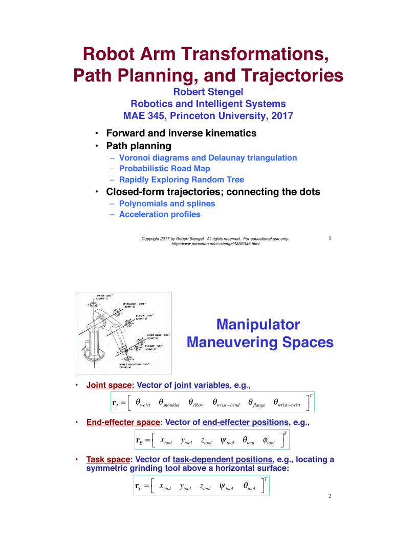
Manipulator Maneuvering Spaces

•! Joint space: Vector of joint variables, e.g.,

rJ = !waist !shoulder !elbow !wrist"bend ! flange !wrist" twist#$

%&T

•! End-effecter space: Vector of end-effecter positions, e.g.,

rE = xtool ytool ztool ! tool "tool #tool$%

&'T

•! Task space: Vector of task-dependent positions, e.g., locating a symmetric grinding tool above a horizontal surface:

rT = xtool ytool ztool ! tool "tool#$

%&T

2

Forward and Inverse Transformations of a Robotic Assembly

Forward TransformationTransforms homogeneous coordinates from tool frame to reference

frame coordinates

Inverse TransformationTransform homogeneous coordinate from reference frame to tool

frame coordinates

sbase = Atoolbasestool

= AwaistAshoulderAelbowAwrist!bendA flangeAwrist!twiststool

stool = Abasetool sbase

= A!1wrist!twistA

!1flangeA

!1wrist!bendA

!1elbowA

!1shoulderA

!1waistsbase

3

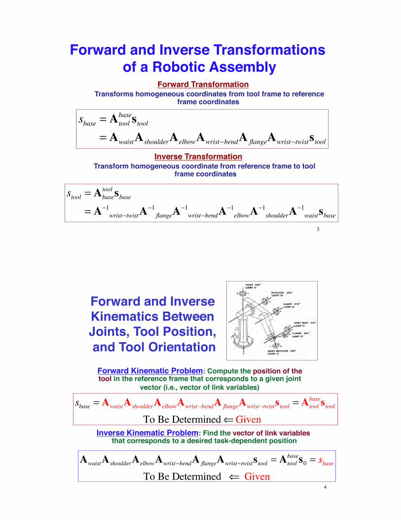
Forward and Inverse Kinematics Between Joints, Tool Position, and Tool Orientation

Forward Kinematic Problem: Compute the position of the tool in the reference frame that corresponds to a given joint

vector (i.e., vector of link variables)

Inverse Kinematic Problem: Find the vector of link variables that corresponds to a desired task-dependent position

sbase = AwaistAshoulderAelbowAwrist!bendA flangeAwrist!twiststool = Atoolbasestool

To Be Determined "Given

AwaistAshoulderAelbowAwrist!bendA flangeAwrist!twiststool = Atoolbases0 = sbase

To Be Determined " Given4

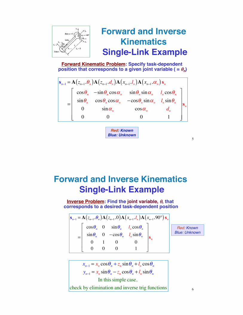
Forward and Inverse Kinematics

Single-Link ExampleForward Kinematic Problem: Specify task-dependent

position that corresponds to a given joint variable ( = !!n)

sn!1 = A zn!1,"n( )A zn!1,dn( )A xn!1,ln( )A xn!1,# n( ) sn

=

cos"n !sin"n cos# n sin"n sin# n ln cos"n

sin"n cos"n cos# n !cos"n sin# n ln sin"n

0 sin# n cos# n dn0 0 0 1

$

%

&&&&&

'

(

)))))

sn

Red: KnownBlue: Unknown

5

Inverse Problem: Find the joint variable, !!, that corresponds to a desired task-dependent position

Red: KnownBlue: Unknown

xn!1 = xn cos"n + zn sin"n + ln cos"n

yn!1 = xn sin"n ! zn cos"n + ln sin"n

In this simple case, check by elimination and inverse trig functions

sn!1 = A zn!1,"n( )A zn!1,0( )A xn!1,ln( )A xn!1,90°( ) sn

=

cos"n 0 sin"n ln cos"n

sin"n 0 !cos"n ln sin"n

0 1 0 00 0 0 1

#

$

%%%%

&

'

((((

sn

Forward and Inverse Kinematics Single-Link Example

6

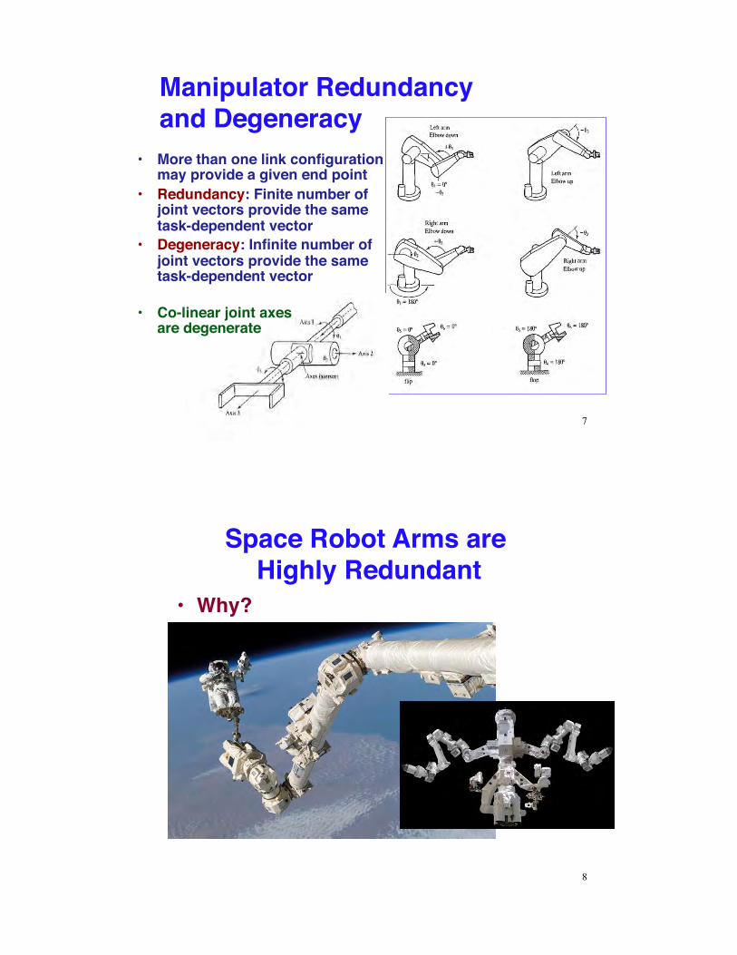
Manipulator Redundancy and Degeneracy

•! More than one link configuration may provide a given end point

•! Redundancy: Finite number of joint vectors provide the same task-dependent vector

•! Degeneracy: Infinite number of joint vectors provide the same task-dependent vector

•! Co-linear joint axes are degenerate

7

Space Robot Arms are Highly Redundant

•! Why?

8

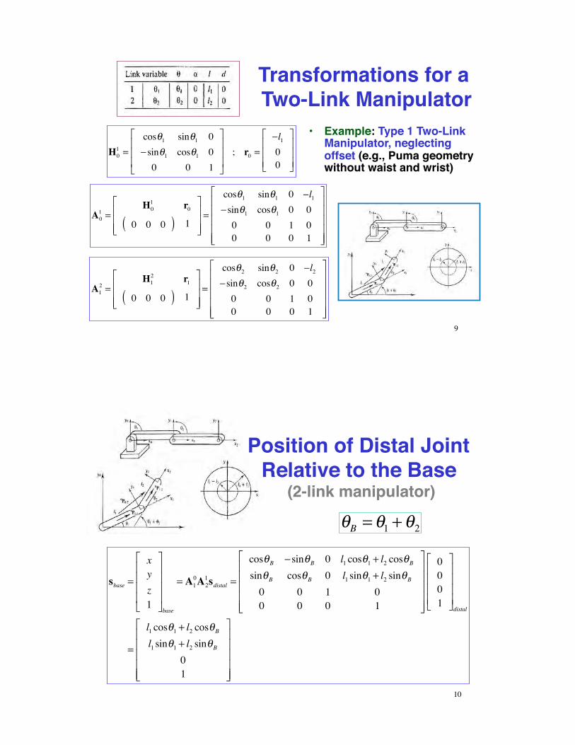
Transformations for a Two-Link Manipulator

•! Example: Type 1 Two-Link Manipulator, neglecting offset (e.g., Puma geometry without waist and wrist)

H01 =

cos!1 sin!1 0" sin!1 cos!1 00 0 1

#

$

%%%

&

'

(((; r0 =

"l100

#

$

%%%

&

'

(((

A01 =

H01 r0

0 0 0( ) 1

!

"

###

$

%

&&&=

cos'1 sin'1 0 (l1(sin'1 cos'1 0 00 0 1 00 0 0 1

!

"

#####

$

%

&&&&&

A12 =

H12 r1

0 0 0( ) 1

!

"

###

$

%

&&&=

cos'2 sin'2 0 (l2(sin'2 cos'2 0 00 0 1 00 0 0 1

!

"

#####

$

%

&&&&&

9

sbase =

xyz1

!

"

####

$

%

&&&&base

= A10A2

1sdistal =

cos'B (sin'B 0 l1 cos'1 + l2 cos'B

sin'B cos'B 0 l1 sin'1 + l2 sin'B

0 0 1 00 0 0 1

!

"

#####

$

%

&&&&&

0001

!

"

####

$

%

&&&&distal

=

l1 cos'1 + l2 cos'B

l1 sin'1 + l2 sin'B

01

!

"

#####

$

%

&&&&&

!B = !1 + !2

Position of Distal Joint Relative to the Base

(2-link manipulator)

10

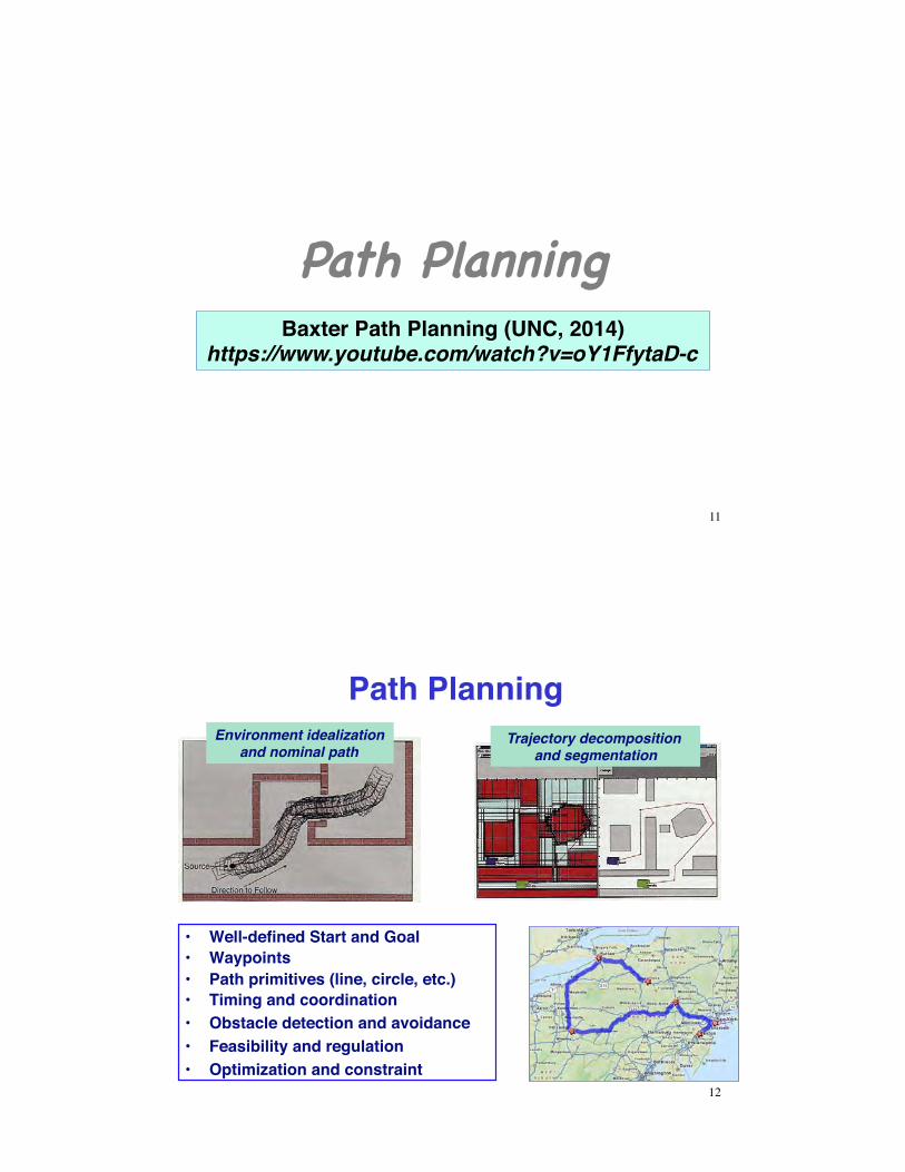
Path Planning!

11

Baxter Path Planning (UNC, 2014)https://www.youtube.com/watch?v=oY1FfytaD-c

Path PlanningTrajectory decomposition

and segmentationEnvironment idealization

and nominal path

•! Well-defined Start and Goal•! Waypoints•! Path primitives (line, circle, etc.)•! Timing and coordination•! Obstacle detection and avoidance•! Feasibility and regulation•! Optimization and constraint

12

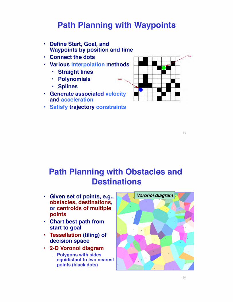
Path Planning with Waypoints

•! Define Start, Goal, and Waypoints by position and time

•! Connect the dots•! Various interpolation methods

•! Straight lines•! Polynomials•! Splines

•! Generate associated velocity and acceleration

•! Satisfy trajectory constraints

13

Path Planning with Obstacles and Destinations

•! Given set of points, e.g., obstacles, destinations, or centroids of multiple points

•! Chart best path from start to goal

•! Tessellation (tiling) of decision space

•! 2-D Voronoi diagram–! Polygons with sides

equidistant to two nearest points (black dots)

Voronoi diagram

14

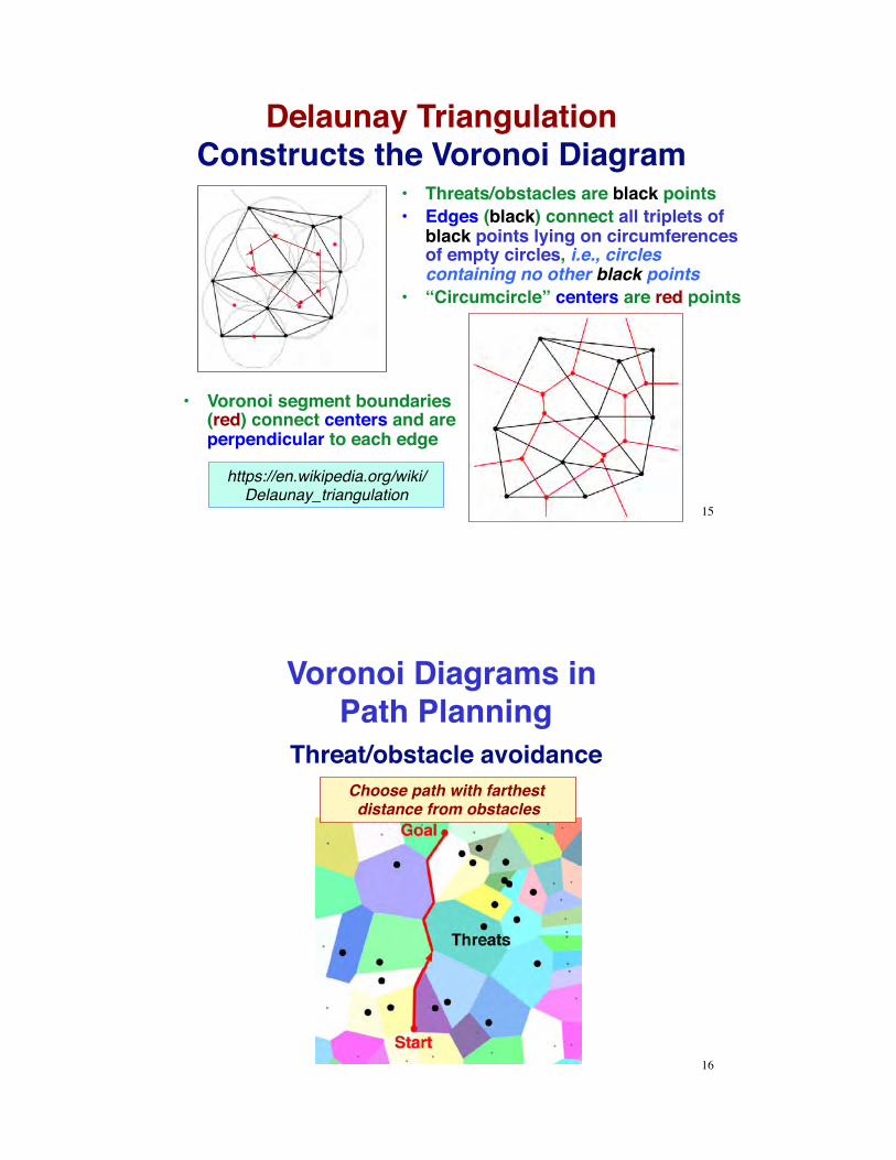
Delaunay Triangulation Constructs the Voronoi Diagram

•! Threats/obstacles are black points•! Edges (black) connect all triplets of

black points lying on circumferences of empty circles, i.e., circles containing no other black points

•! “Circumcircle” centers are red points

15

•! Voronoi segment boundaries (red) connect centers and are perpendicular to each edge

https://en.wikipedia.org/wiki/Delaunay_triangulation

Voronoi Diagrams in Path Planning

Threat/obstacle avoidance

16

Choose path with farthest distance from obstacles

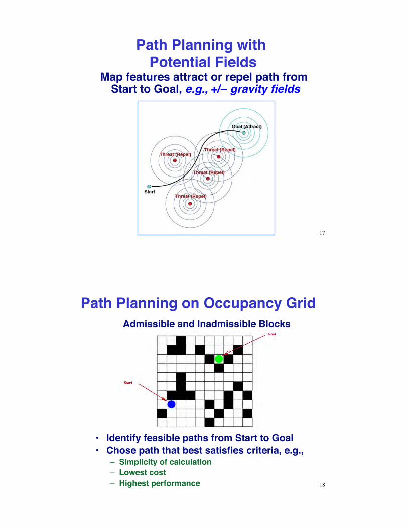
Path Planning with Potential Fields

Map features attract or repel path from Start to Goal, e.g., +/– gravity fields

17

Path Planning on Occupancy Grid

18

Admissible and Inadmissible Blocks

•! Identify feasible paths from Start to Goal•! Chose path that best satisfies criteria, e.g.,

–! Simplicity of calculation–! Lowest cost–! Highest performance

19

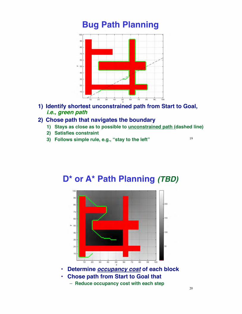
1)" Identify shortest unconstrained path from Start to Goal, i.e., green path

2)" Chose path that navigates the boundary1)" Stays as close as to possible to unconstrained path (dashed line)2)" Satisfies constraint3)" Follows simple rule, e.g., “stay to the left”

Bug Path Planning

D* or A* Path Planning (TBD)

20

•! Determine occupancy cost of each block•! Chose path from Start to Goal that

–! Reduce occupancy cost with each step

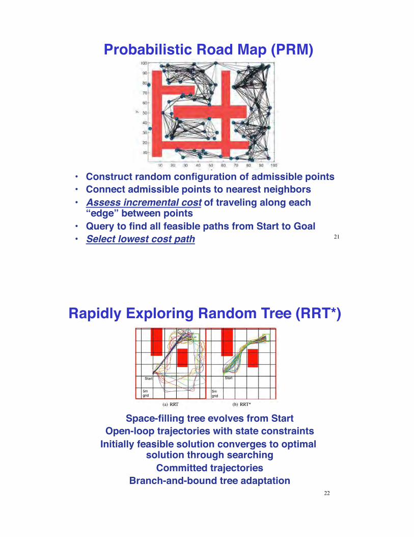
Probabilistic Road Map (PRM)

•! Construct random configuration of admissible points•! Connect admissible points to nearest neighbors•! Assess incremental cost of traveling along each

“edge” between points•! Query to find all feasible paths from Start to Goal•! Select lowest cost path 21

Rapidly Exploring Random Tree (RRT*)

Space-filling tree evolves from StartOpen-loop trajectories with state constraints

Initially feasible solution converges to optimal solution through searching

Committed trajectoriesBranch-and-bound tree adaptation

22

Trajectories!

23

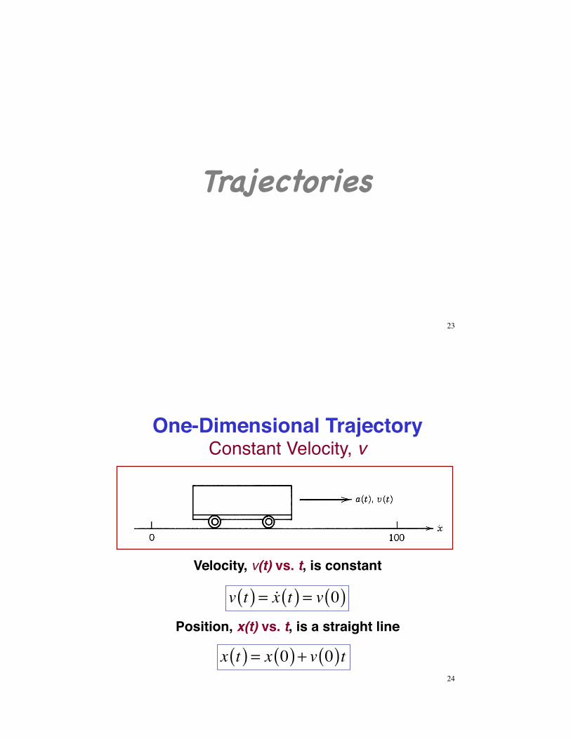
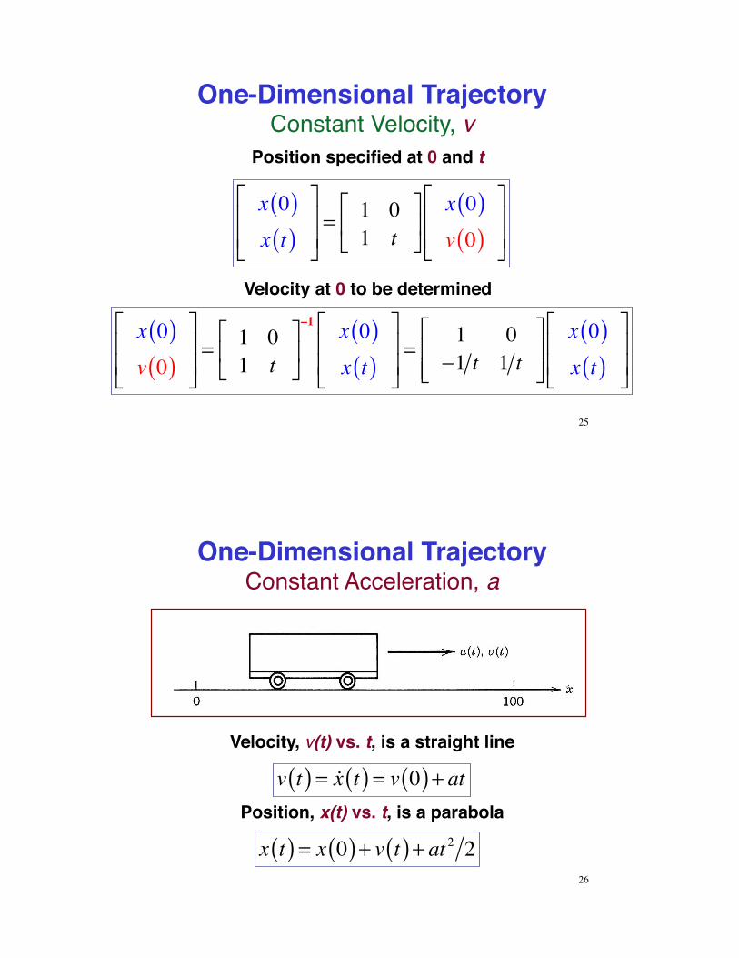
One-Dimensional TrajectoryConstant Velocity, v

24

Position, x(t) vs. t, is a straight line

Velocity, v(t) vs. t, is constant

x t( ) = x 0( ) + v 0( )t

v t( ) = !x t( ) = v 0( )

One-Dimensional TrajectoryConstant Velocity, v

25

Position specified at 0 and t

x 0( )x t( )

!

"##

$

%&&= 1 0

1 t!

"#

$

%&

x 0( )v 0( )

!

"##

$

%&&

Velocity at 0 to be determined

x 0( )v 0( )

!

"##

$

%&&= 1 0

1 t!

"#

$

%&

–1 x 0( )x t( )

!

"##

$

%&&=

1 0'1 t 1 t

!

"##

$

%&&

x 0( )x t( )

!

"##

$

%&&

One-Dimensional TrajectoryConstant Acceleration, a

26

Position, x(t) vs. t, is a parabola

Velocity, v(t) vs. t, is a straight line

x t( ) = x 0( ) + v t( ) + at 2 2

v t( ) = !x t( ) = v 0( ) + at

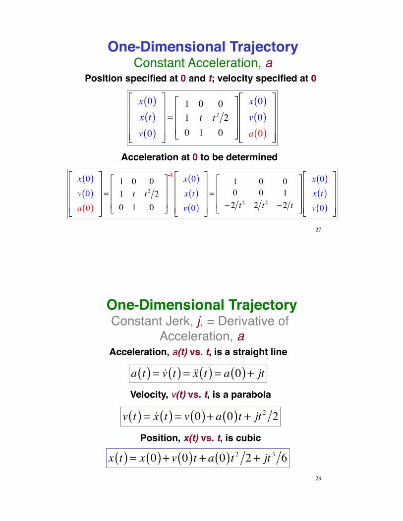
One-Dimensional TrajectoryConstant Acceleration, a

27

Position specified at 0 and t; velocity specified at 0

x 0( )x t( )v 0( )

!

"

####

$

%

&&&&

=1 0 01 t t 2 20 1 0

!

"

###

$

%

&&&

x 0( )v 0( )a 0( )

!

"

####

$

%

&&&&

Acceleration at 0 to be determined

x 0( )v 0( )a 0( )

!

"

####

$

%

&&&&

=1 0 01 t t 2 20 1 0

!

"

###

$

%

&&&

–1 x 0( )x t( )v 0( )

!

"

####

$

%

&&&&

=1 0 00 0 1

'2 t 2 2 t 2 '2 t

!

"

###

$

%

&&&

x 0( )x t( )v 0( )

!

"

####

$

%

&&&&

One-Dimensional TrajectoryConstant Jerk, j, = Derivative of

Acceleration, a

28

Position, x(t) vs. t, is cubic

Velocity, v(t) vs. t, is a parabola

x t( ) = x 0( ) + v 0( )t + a 0( )t 2 2 + jt 3 6

v t( ) = !x t( ) = v 0( ) + a 0( )t + jt 2 2

Acceleration, a(t) vs. t, is a straight line

a t( ) = !v t( ) = !!x t( ) = a 0( ) + jt

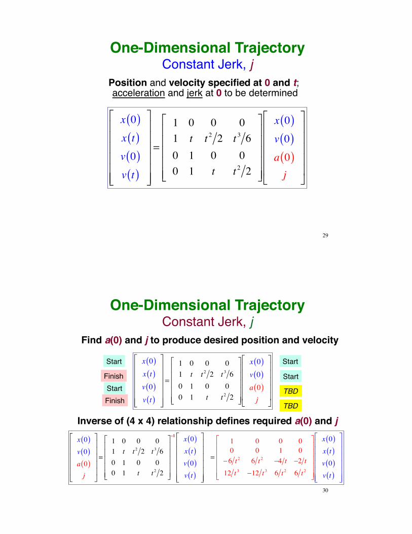
One-Dimensional TrajectoryConstant Jerk, j

29

Position and velocity specified at 0 and t; acceleration and jerk at 0 to be determined

x 0( )x t( )v 0( )v t( )

!

"

######

$

%

&&&&&&

=

1 0 0 01 t t 2 2 t 3 60 1 0 00 1 t t 2 2

!

"

#####

$

%

&&&&&

x 0( )v 0( )a 0( )j

!

"

#####

$

%

&&&&&

One-Dimensional TrajectoryConstant Jerk, j

30

Find a(0) and j to produce desired position and velocity

x 0( )x t( )v 0( )v t( )

!

"

######

$

%

&&&&&&

=

1 0 0 01 t t 2 2 t 3 60 1 0 00 1 t t 2 2

!

"

#####

$

%

&&&&&

x 0( )v 0( )a 0( )j

!

"

#####

$

%

&&&&&

x 0( )v 0( )a 0( )j

!

"

#####

$

%

&&&&&

=

1 0 0 01 t t 2 2 t 3 60 1 0 00 1 t t 2 2

!

"

#####

$

%

&&&&&

–1 x 0( )x t( )v 0( )v t( )

!

"

######

$

%

&&&&&&

=

1 0 0 00 0 1 0

'6 t 2 6 t 2 '4 t '2 t

12 t 3 '12 t 3 6 t 2 6 t 2

!

"

#####

$

%

&&&&&

x 0( )x t( )v 0( )v t( )

!

"

######

$

%

&&&&&&

Inverse of (4 x 4) relationship defines required a(0) and j

Start

Start

Finish

Finish

Start

Start

TBD

TBD

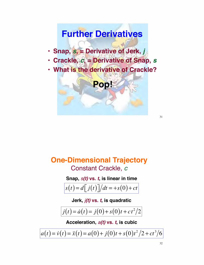
Further Derivatives•! Snap, s, = Derivative of Jerk, j•! Crackle, c, = Derivative of Snap, s•! What is the derivative of Crackle?

31

Pop!

One-Dimensional TrajectoryConstant Crackle, c

32

Acceleration, a(t) vs. t, is cubic

a t( ) = !v t( ) = !!x t( ) = a 0( ) + j 0( )t + s 0( )t 2 2 + ct 3 6

Jerk, j(t) vs. t, is quadratic

j t( ) = !a t( ) = j 0( ) + s 0( )t + ct 2 2

Snap, s(t) vs. t, is linear in time

s t( ) = d j t( )!" #$ dt = +s 0( ) + ct

33

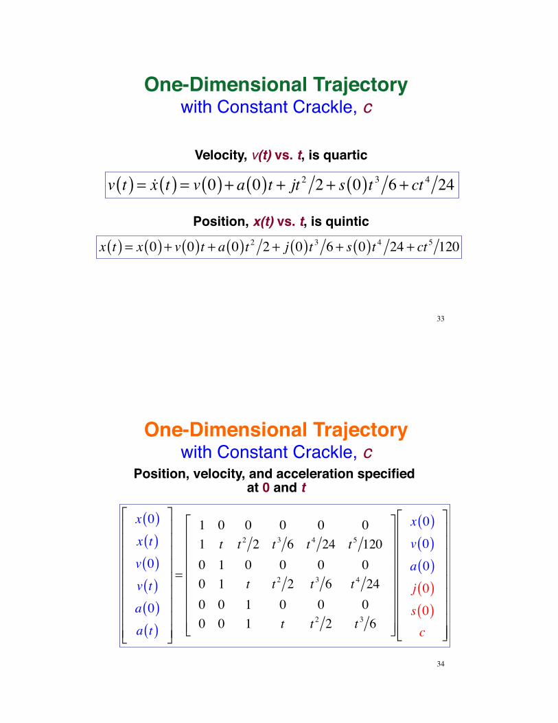
Position, x(t) vs. t, is quintic

Velocity, v(t) vs. t, is quartic

x t( ) = x 0( ) + v 0( )t + a 0( )t 2 2 + j 0( )t 3 6 + s 0( )t 4 24 + ct 5 120

v t( ) = !x t( ) = v 0( ) + a 0( )t + jt 2 2 + s 0( )t 3 6 + ct 4 24

One-Dimensional Trajectorywith Constant Crackle, c

34

Position, velocity, and acceleration specified at 0 and t

x 0( )x t( )v 0( )v t( )a 0( )a t( )

!

"

#########

$

%

&&&&&&&&&

=

1 0 0 0 0 01 t t 2 2 t 3 6 t 4 24 t 5 1200 1 0 0 0 00 1 t t 2 2 t 3 6 t 4 240 0 1 0 0 00 0 1 t t 2 2 t 3 6

!

"

########

$

%

&&&&&&&&

x 0( )v 0( )a 0( )j 0( )s 0( )c

!

"

#########

$

%

&&&&&&&&&

One-Dimensional Trajectorywith Constant Crackle, c

35

x 0( )v 0( )a 0( )j 0( )s 0( )c

!

"

#########

$

%

&&&&&&&&&

=

1 0 0 0 0 01 t t 2 2 t 3 6 t 4 24 t 5 1200 1 0 0 0 00 1 t t 2 2 t 3 6 t 4 240 0 1 0 0 00 0 1 t t 2 2 t 3 6

!

"

########

$

%

&&&&&&&&

–1 x 0( )x t( )v 0( )v t( )a 0( )a t( )

!

"

#########

$

%

&&&&&&&&&

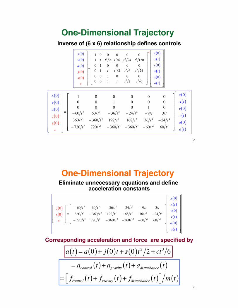
One-Dimensional TrajectoryInverse of (6 x 6) relationship defines controls

x 0( )v 0( )a 0( )j 0( )s 0( )c

!

"

#########

$

%

&&&&&&&&&

=

1 0 0 0 0 00 0 1 0 0 00 0 0 0 1 0

'60 t 3 60 t 3 ' 36 t 2 '24 t 2 '9 t 3 t

360 t 4 ' 360 t 4 192 t 3 168 t 3 36 t 2 '24 t 2

' 720 t 5 720 t 5 ' 360 t 4 ' 360 t 4 '60 t 3 60 t 3

!

"

########

$

%

&&&&&&&&

x 0( )x t( )v 0( )v t( )a 0( )a t( )

!

"

#########

$

%

&&&&&&&&&

36

One-Dimensional TrajectoryEliminate unnecessary equations and define

acceleration constants

j 0( )s 0( )c

!

"

###

$

%

&&&=

'60 t 3 60 t 3 ' 36 t 2 '24 t 2 '9 t 3 t

360 t 4 ' 360 t 4 192 t 3 168 t 3 36 t 2 '24 t 2

' 720 t 5 720 t 5 ' 360 t 4 ' 360 t 4 '60 t 3 60 t 3

!

"

####

$

%

&&&&

x 0( )x t( )v 0( )v t( )a 0( )a t( )

!

"

#########

$

%

&&&&&&&&&

a t( ) = a 0( ) + j 0( )t + s 0( )t 2 2 + ct 3 6Corresponding acceleration and force are specified by

= acontrol t( ) + agravity t( ) + adisturbance t( )= fcontrol t( ) + fgravity t( ) + fdisturbance t( )!" #$ m t( )

37

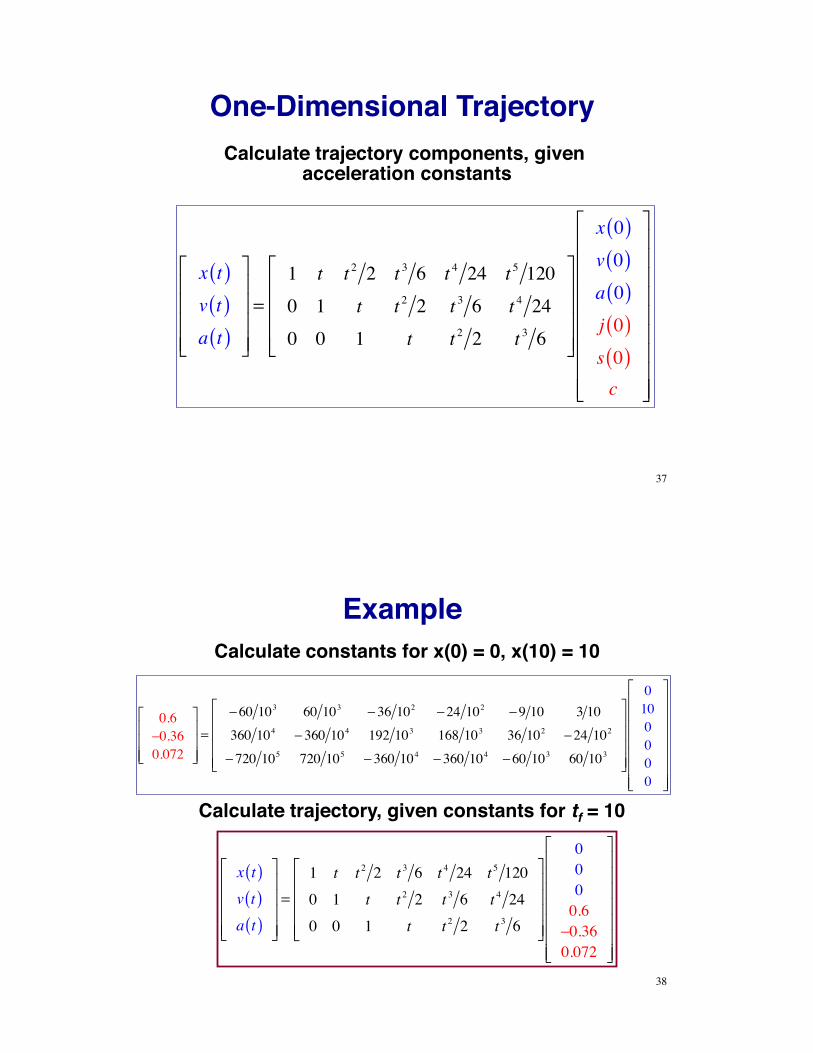
One-Dimensional TrajectoryCalculate trajectory components, given

acceleration constants

x t( )v t( )a t( )

!

"

####

$

%

&&&&

=

1 t t 2 2 t 3 6 t 4 24 t 5 120

0 1 t t 2 2 t 3 6 t 4 24

0 0 1 t t 2 2 t 3 6

!

"

####

$

%

&&&&

x 0( )v 0( )a 0( )j 0( )s 0( )c

!

"

#########

$

%

&&&&&&&&&

38

Example

x t( )v t( )a t( )

!

"

####

$

%

&&&&

=

1 t t 2 2 t 3 6 t 4 24 t 5 120

0 1 t t 2 2 t 3 6 t 4 24

0 0 1 t t 2 2 t 3 6

!

"

####

$

%

&&&&

0000.6

'0.360.072

!

"

#######

$

%

&&&&&&&

0.6!0.360.072

"

#

$$$

%

&

'''=

!60 103 60 103 ! 36 102 !24 102 !9 10 3 10

360 104 ! 360 104 192 103 168 103 36 102 !24 102

! 720 105 720 105 ! 360 104 ! 360 104 !60 103 60 103

"

#

$$$$

%

&

''''

0100000

"

#

$$$$$$$

%

&

'''''''

Calculate constants for x(0) = 0, x(10) = 10

Calculate trajectory, given constants for tf = 10

39

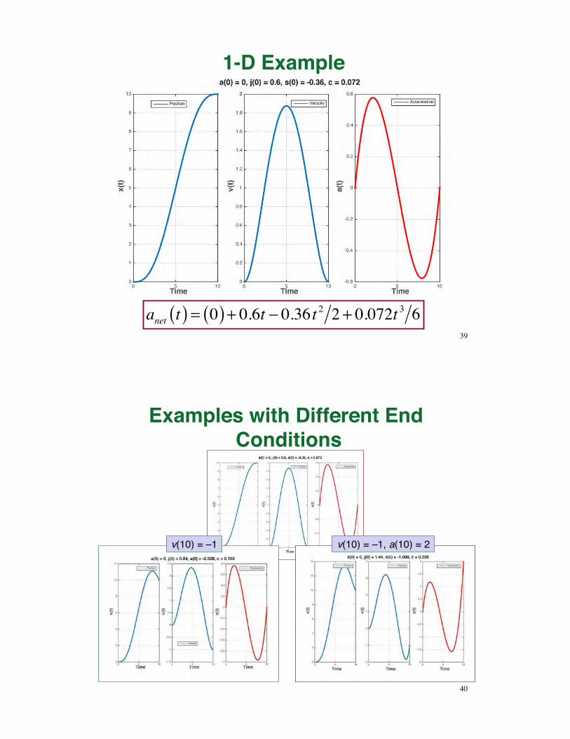
1-D Example

anet t( ) = 0( ) + 0.6t ! 0.36 t 2 2 + 0.072t 3 6

40

Examples with Different End Conditions

v(10) = –1 v(10) = –1, a(10) = 2

41

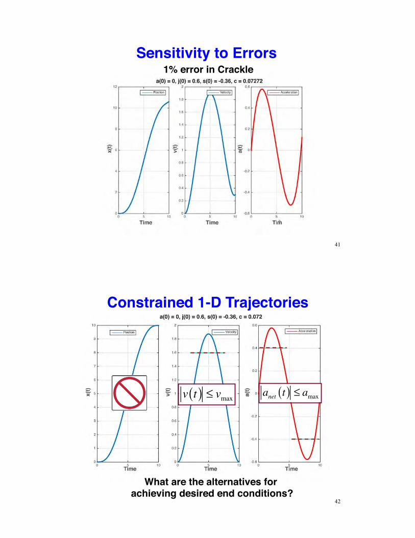
Sensitivity to Errors1% error in Crackle

42

Constrained 1-D Trajectories

anet t( ) ! amaxv t( ) ! vmax

What are the alternatives for achieving desired end conditions?

43

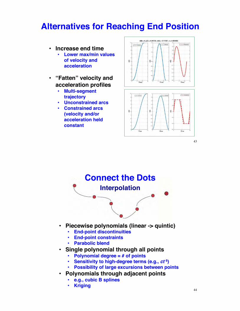
Alternatives for Reaching End Position

•! Increase end time•! Lower max/min values

of velocity and acceleration

•! “Fatten” velocity and acceleration profiles•! Multi-segment

trajectory•! Unconstrained arcs•! Constrained arcs

(velocity and/or acceleration held constant

44

Interpolation

•! Piecewise polynomials (linear -> quintic)•! End-point discontinuities•! End-point constraints•! Parabolic blend

•! Single polynomial through all points•! Polynomial degree = # of points•! Sensitivity to high-degree terms (e.g., ct 6)•! Possibility of large excursions between points

•! Polynomials through adjacent points•! e.g., cubic B splines•! Kriging

Connect the Dots

Next Time:!Time Response of Dynamic Systems!

45

SSuupppplleemmeennttaall MMaatteerriiaall

46

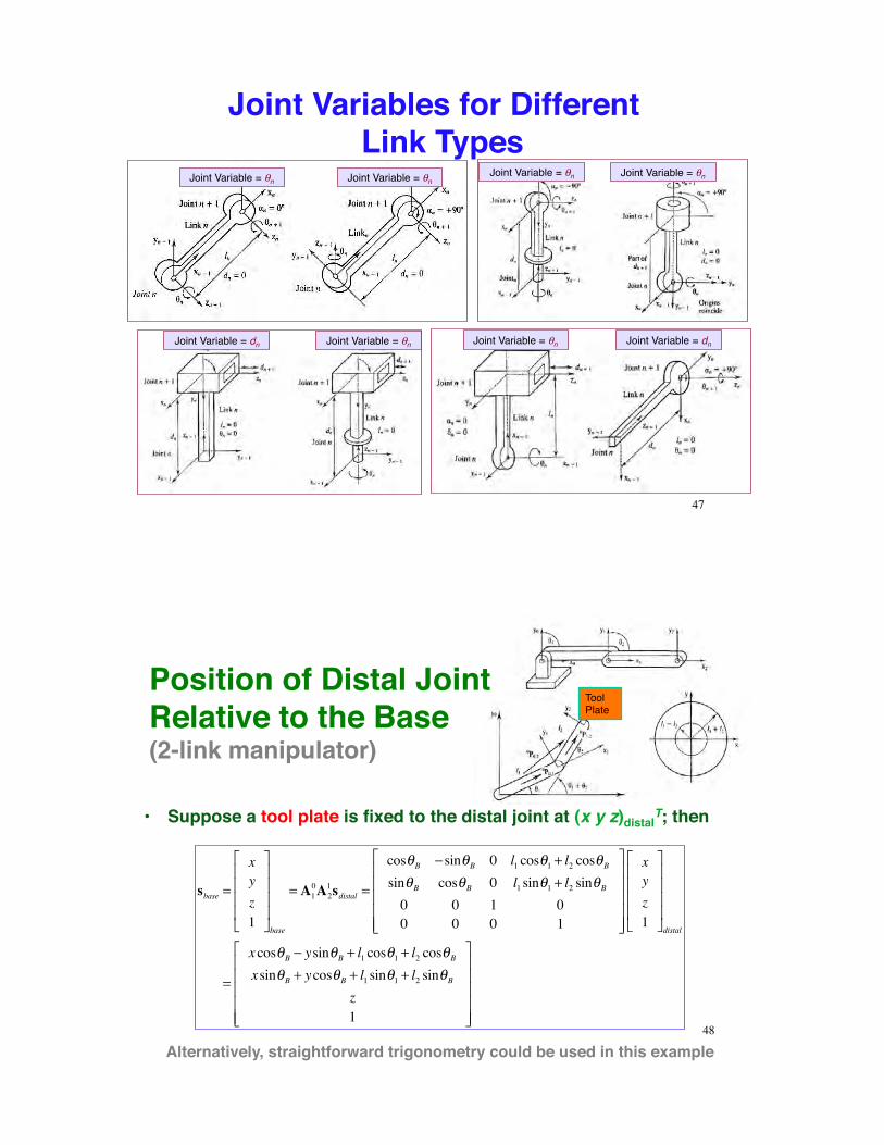
Joint Variables for Different Link Types

Joint Variable = !n Joint Variable = !n

Joint Variable = !n

Joint Variable = !nJoint Variable = !n

Joint Variable = !nJoint Variable = dn Joint Variable = dn

47

•! Suppose a tool plate is fixed to the distal joint at (x y z)distalT; then

sbase =

xyz1

!

"

####

$

%

&&&&base

= A10A2

1sdistal =

cos'B (sin'B 0 l1 cos'1 + l2 cos'B

sin'B cos'B 0 l1 sin'1 + l2 sin'B

0 0 1 00 0 0 1

!

"

#####

$

%

&&&&&

xyz1

!

"

####

$

%

&&&&distal

=

xcos'B ( ysin'B + l1 cos'1 + l2 cos'B

xsin'B + ycos'B + l1 sin'1 + l2 sin'B

z1

!

"

#####

$

%

&&&&&

Alternatively, straightforward trigonometry could be used in this example

Tool Plate

Position of Distal Joint Relative to the Base (2-link manipulator)

48

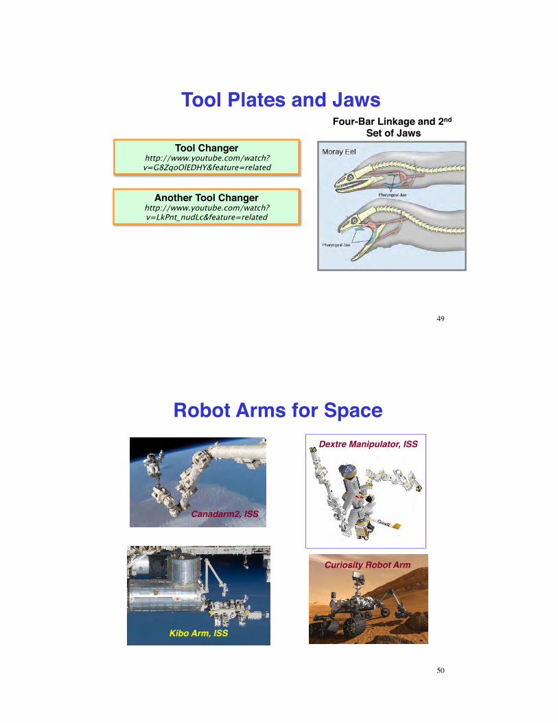
Tool Plates and Jaws

Tool Changerhttp://www.youtube.com/watch?v=G8ZqoOlEDHY&feature=related

Another Tool Changerhttp://www.youtube.com/watch?v=LkPnt_nudLc&feature=related

49

Four-Bar Linkage and 2nd Set of Jaws

Robot Arms for SpaceDextre Manipulator, ISS

Canadarm2, ISS

Curiosity Robot Arm

Kibo Arm, ISS

50

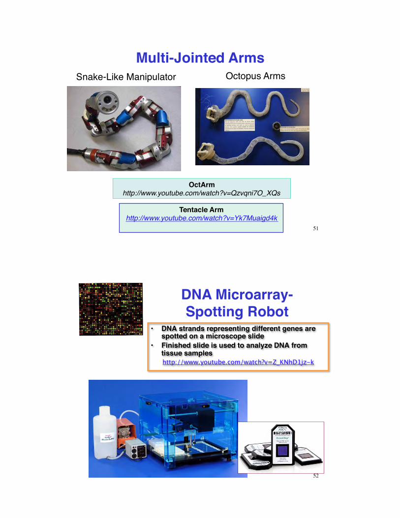
Multi-Jointed ArmsOctopus ArmsSnake-Like Manipulator

OctArmhttp://www.youtube.com/watch?v=Qzvqni7O_XQs

Tentacle Armhttp://www.youtube.com/watch?v=Yk7Muaigd4k

51

DNA Microarray-Spotting Robot

•! DNA strands representing different genes are spotted on a microscope slide

•! Finished slide is used to analyze DNA from tissue sampleshttp://www.youtube.com/watch?v=Z_KNhD1jz-k

52

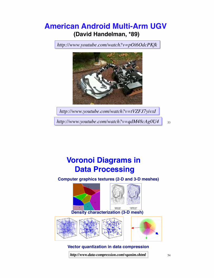
American Android Multi-Arm UGV (David Handelman, *89)

http://www.youtube.com/watch?v=pOi6OdcPKfk

http://www.youtube.com/watch?v=tVZFJ7yivxI

http://www.youtube.com/watch?v=qdM48cAg0U4 53

Voronoi Diagrams in Data Processing

Computer graphics textures (2-D and 3-D meshes)

http://www.data-compression.com/vqanim.shtml

Vector quantization in data compression

Density characterization (3-D mesh)

54

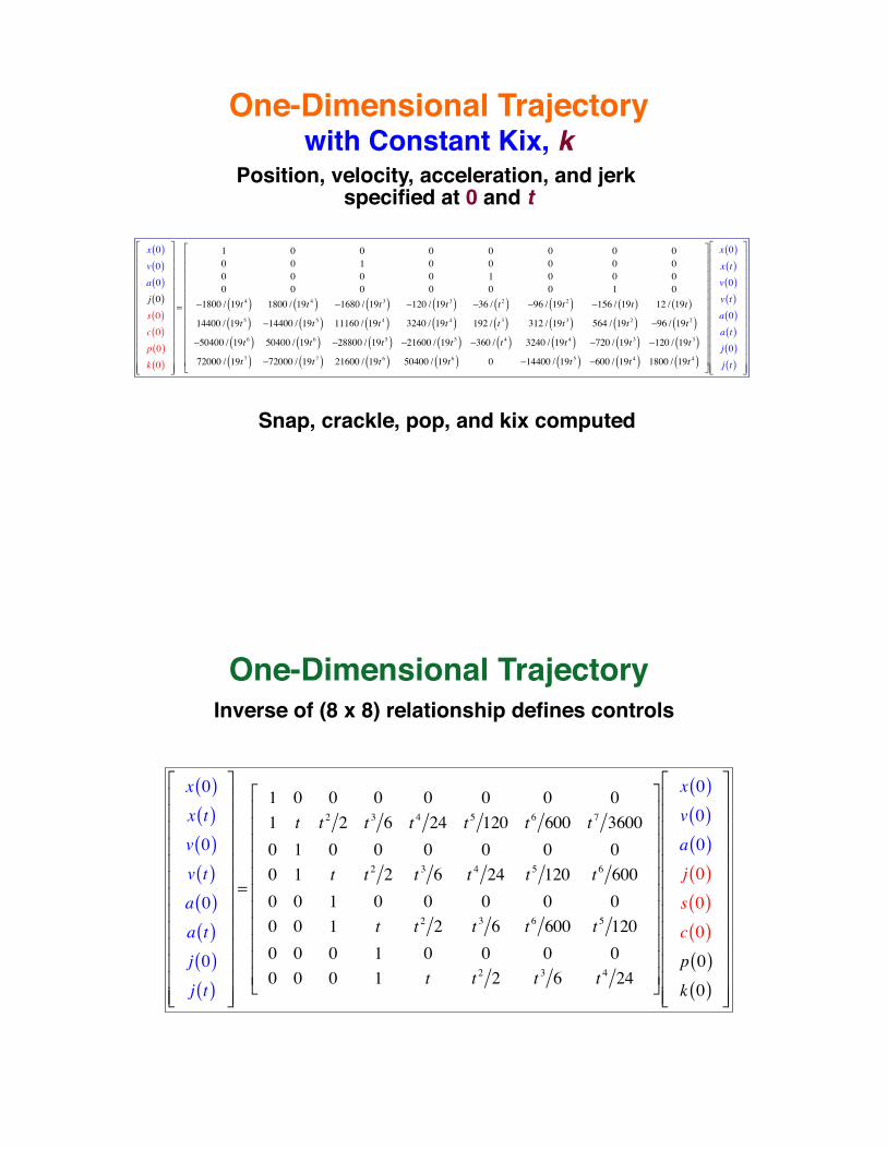
x 0( )v 0( )a 0( )j 0( )s 0( )c 0( )p 0( )k 0( )

!

"

#############

$

%

&&&&&&&&&&&&&

=

1 0 0 0 0 0 0 00 0 1 0 0 0 0 00 0 0 0 1 0 0 00 0 0 0 0 0 1 0

'1800 / 19t 4( ) 1800 / 19t 4( ) '1680 / 19t 3( ) '120 / 19t 3( ) '36 / t 2( ) '96 / 19t 2( ) '156 / 19t( ) 12 / 19t( )14400 / 19t 5( ) '14400 / 19t 5( ) 11160 / 19t 4( ) 3240 / 19t 4( ) 192 / t 3( ) 312 / 19t 3( ) 564 / 19t 2( ) '96 / 19t 2( )'50400 / 19t 6( ) 50400 / 19t 6( ) '28800 / 19t 5( ) '21600 / 19t 5( ) '360 / t 4( ) 3240 / 19t 4( ) '720 / 19t 3( ) '120 / 19t 3( )72000 / 19t 7( ) '72000 / 19t 7( ) 21600 / 19t 6( ) 50400 / 19t 6( ) 0 '14400 / 19t 5( ) '600 / 19t 4( ) 1800 / 19t 4( )

!

"

############

$

%

&&&&&&&&&&&&

x 0( )x t( )v 0( )v t( )a 0( )a t( )j 0( )j t( )

!

"

#############

$

%

&&&&&&&&&&&&&

Position, velocity, acceleration, and jerk specified at 0 and t

One-Dimensional Trajectorywith Constant Kix, k

Snap, crackle, pop, and kix computed

x 0( )x t( )v 0( )v t( )a 0( )a t( )j 0( )j t( )

!

"

#############

$

%

&&&&&&&&&&&&&

=

1 0 0 0 0 0 0 01 t t 2 2 t 3 6 t 4 24 t 5 120 t 6 600 t 7 36000 1 0 0 0 0 0 00 1 t t 2 2 t 3 6 t 4 24 t 5 120 t 6 6000 0 1 0 0 0 0 00 0 1 t t 2 2 t 3 6 t 6 600 t 5 1200 0 0 1 0 0 0 00 0 0 1 t t 2 2 t 3 6 t 4 24

!

"

###########

$

%

&&&&&&&&&&&

x 0( )v 0( )a 0( )j 0( )s 0( )c 0( )p 0( )k 0( )

!

"

#############

$

%

&&&&&&&&&&&&&

One-Dimensional TrajectoryInverse of (8 x 8) relationship defines controls