Homogeneous Coordinates (Projective Space)

• Let be a point in Euclidean space

• Change to homogeneous coordinates:

• Defined up to scale:

• Can go back to non-homogeneous representation as follows:

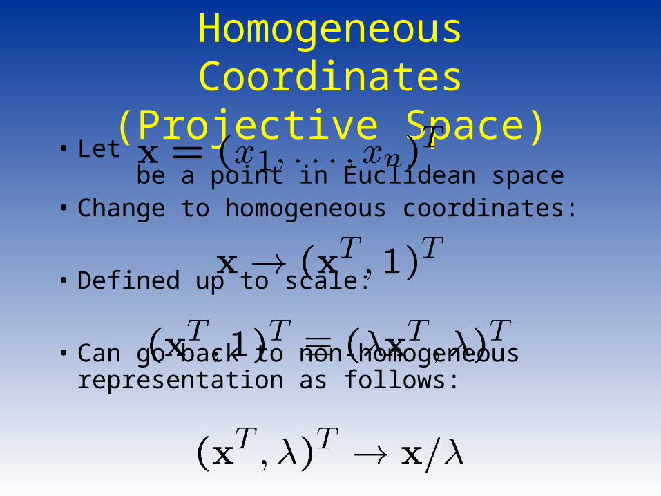
3-D Transformations:Translation

• Ordinarily, a translation between points is expressed as a vector addition

• Homogeneous coordinates allow it to be written as a matrix multiplication:

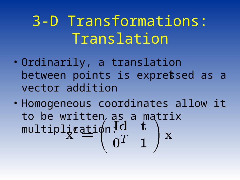
3-D Rotations: Euler Angles

• Can decompose rotation of about arbi-trary 3-D axis into rotations

about the coordinate axes (“yaw-roll-pitch”)

• , where:

(Clockwise when looking toward the origin)

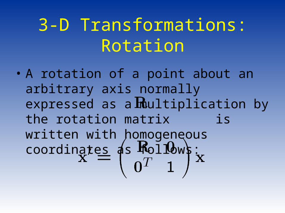
3-D Transformations:Rotation

• A rotation of a point about an arbitrary axis normally expressed as a multiplication by the rotation matrix is written with homogeneous coordinates as follows:

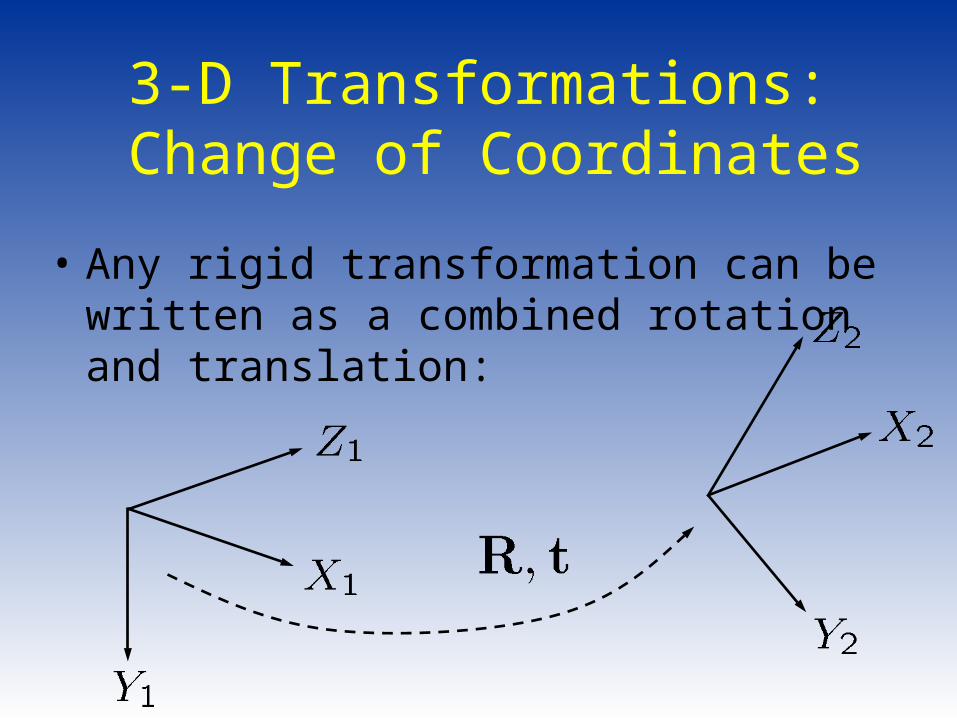
3-D Transformations: Change of Coordinates

• Any rigid transformation can be written as a combined rotation and translation:

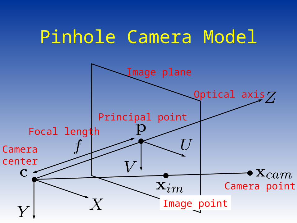
Pinhole Camera Model

Cameracenter

Principal point

Image point

Camera point

Image plane

Focal length

Optical axis

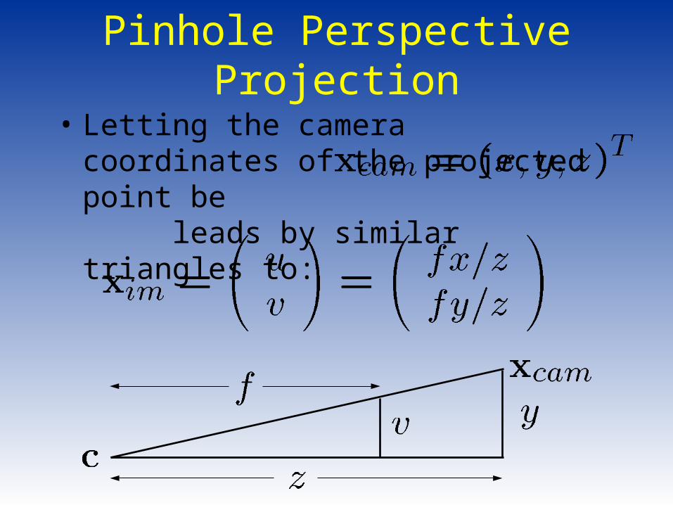
Pinhole Perspective Projection

• Letting the camera coordinates of the projected point be leads by similar triangles to:

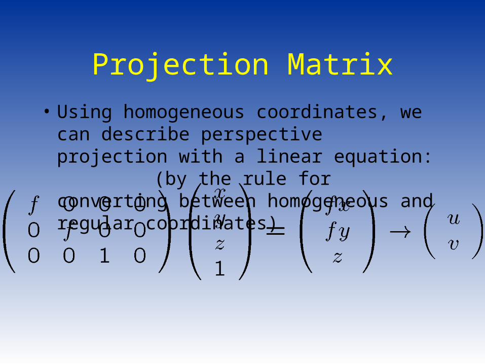
Projection Matrix

• Using homogeneous coordinates, we can describe perspective projection with a linear equation:

(by the rule for converting between homogeneous and regular coordinates)

Example 1: 2D Translation

• Q: How can we represent translation as a 3x3 matrix?

• A: Using the rightmost column:

100

10

01

y

x

t

t

ranslationT

y

x

tyy

txx

'

'

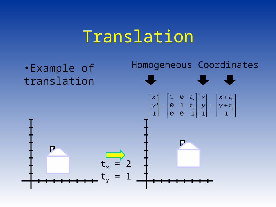
Translation

•Example of translation

11100

10

01

1

'

'

y

x

y

x

ty

tx

y

x

t

t

y

x

tx = 2ty = 1

Homogeneous Coordinates

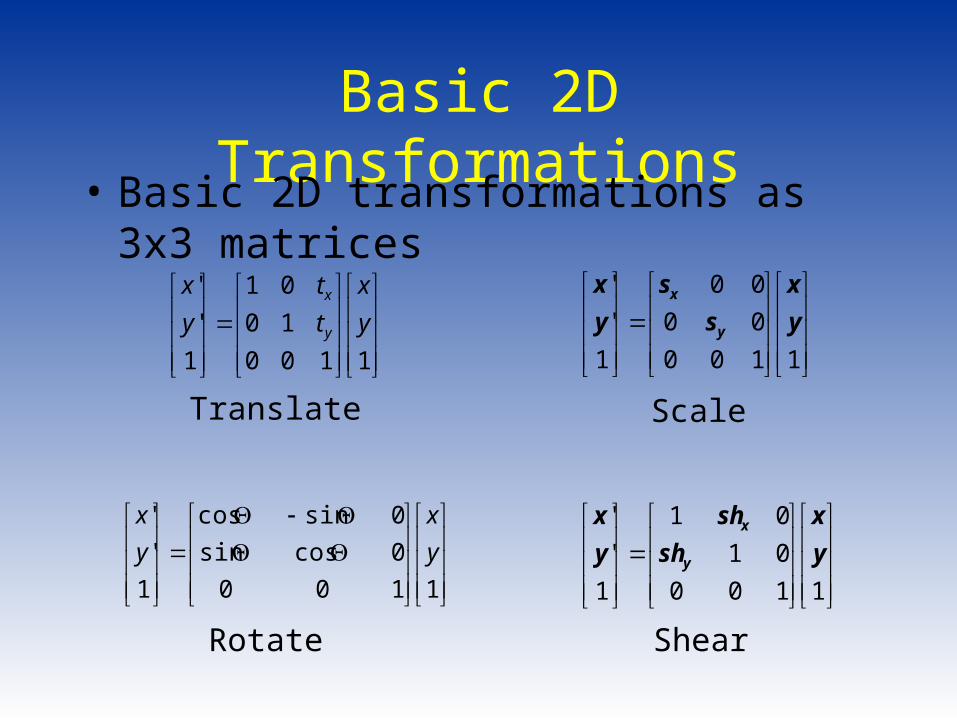
Basic 2D Transformations• Basic 2D transformations as 3x3

matrices

1100

0cossin

0sincos

1

'

'

y

x

y

x

1100

10

01

1

'

'

y

x

t

t

y

x

y

x

1100

01

01

1

'

'

y

x

sh

sh

y

x

y

x

Translate

Rotate Shear

1100

00

00

1

'

'

y

x

s

s

y

x

y

x

Scale

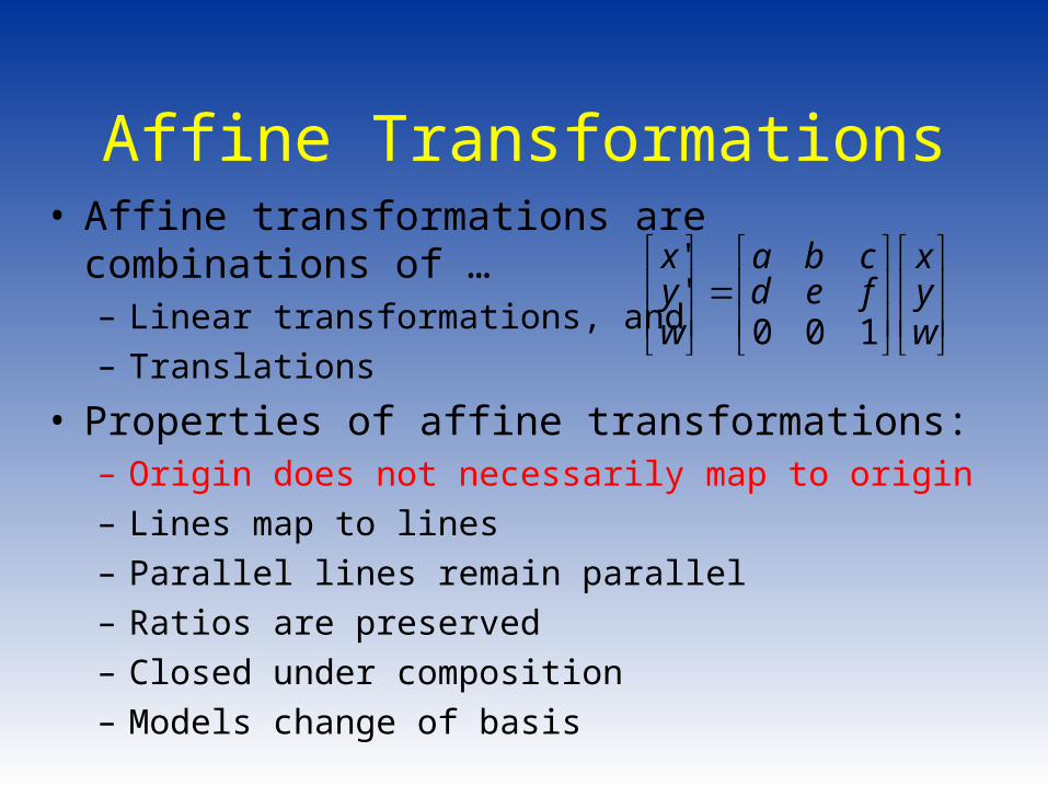
Affine Transformations• Affine transformations are combinations of

…– Linear transformations, and– Translations

• Properties of affine transformations:– Origin does not necessarily map to origin– Lines map to lines– Parallel lines remain parallel– Ratios are preserved– Closed under composition– Models change of basis

wyx

fedcba

wyx

100''

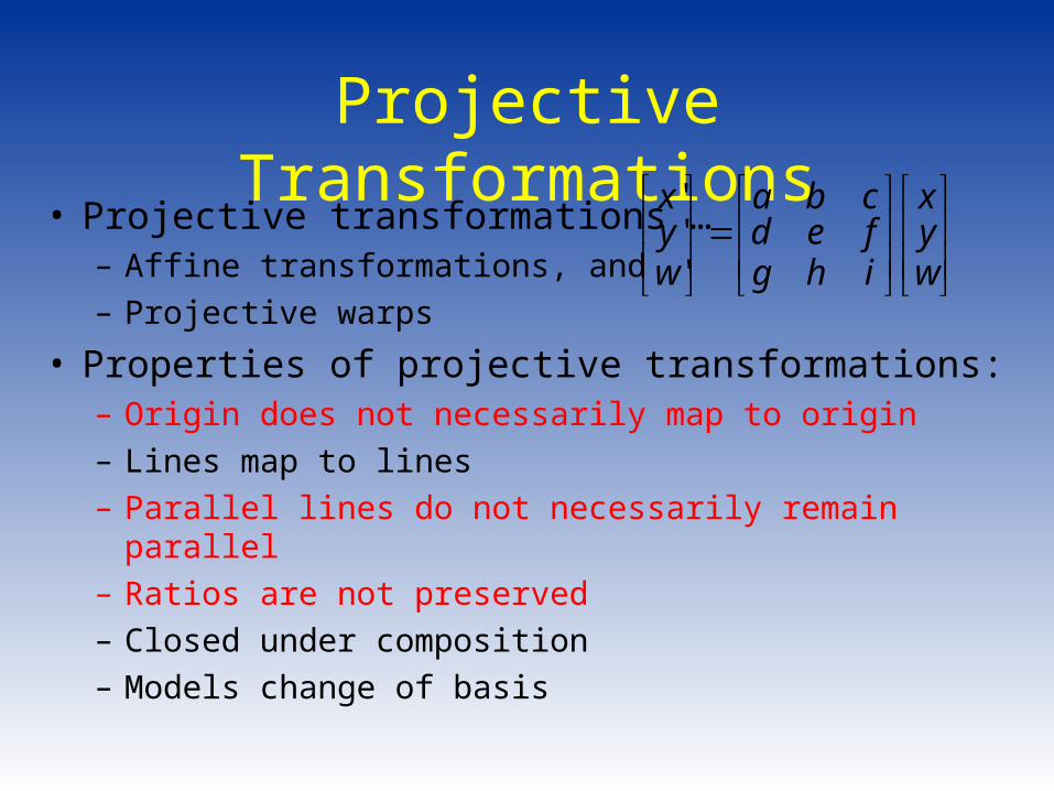
Projective Transformations• Projective transformations …

– Affine transformations, and– Projective warps

• Properties of projective transformations:– Origin does not necessarily map to origin– Lines map to lines– Parallel lines do not necessarily remain parallel– Ratios are not preserved– Closed under composition– Models change of basis

wyx

ihgfedcba

wyx

'''

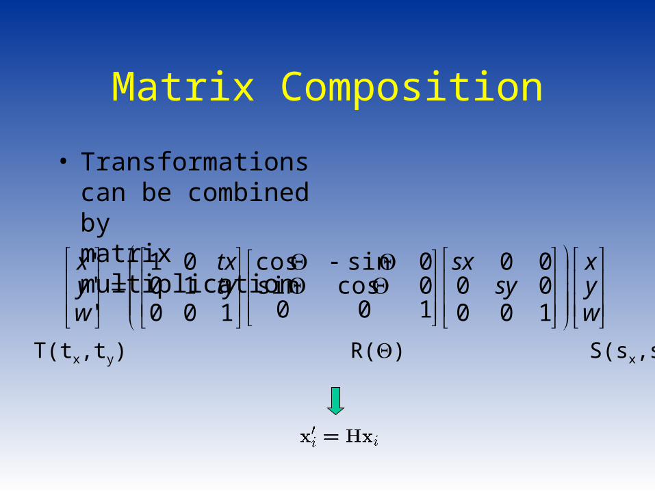
Matrix Composition

• Transformations can be combined by matrix multiplication

wyx

sysx

tytx

wyx

1000000

1000cossin0sincos

1001001

'''

p’ = T(tx,ty) R() S(sx,sy) p

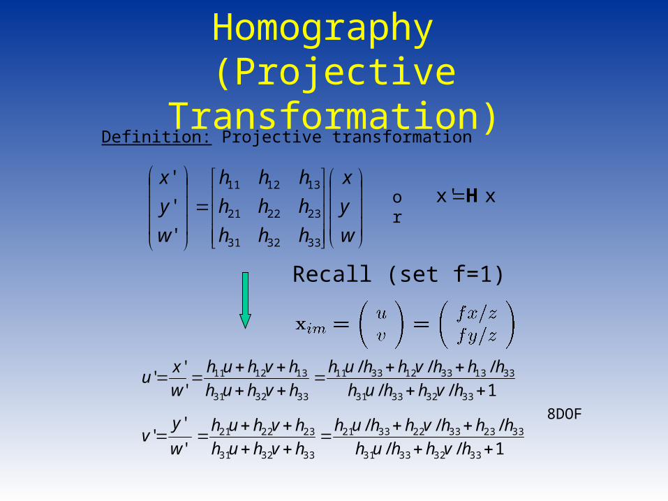
Homography (Projective Transformation)

Definition: Projective transformation

w

y

x

hhh

hhh

hhh

w

y

x

333231

232221

131211

'

'

'xx' Hor

8DOF

1//

///

'

''

33323331

331333123311

333231

131211

hvhhuh

hhhvhhuh

hvhuh

hvhuh

w

xu

1//

///

'

''

33323331

332333223321

333231

232221

hvhhuh

hhhvhhuh

hvhuh

hvhuh

w

yv

Recall (set f=1)

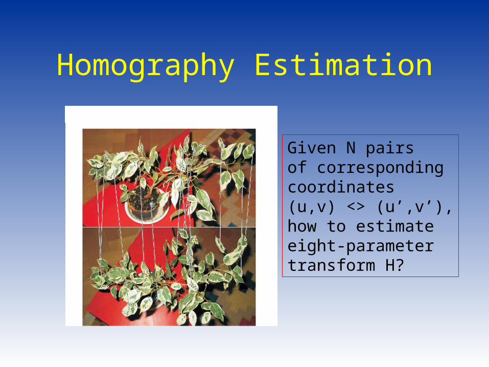
Homography Estimation

Given N pairs of correspondingcoordinates (u,v) <> (u’,v’),how to estimateeight-parametertransform H?

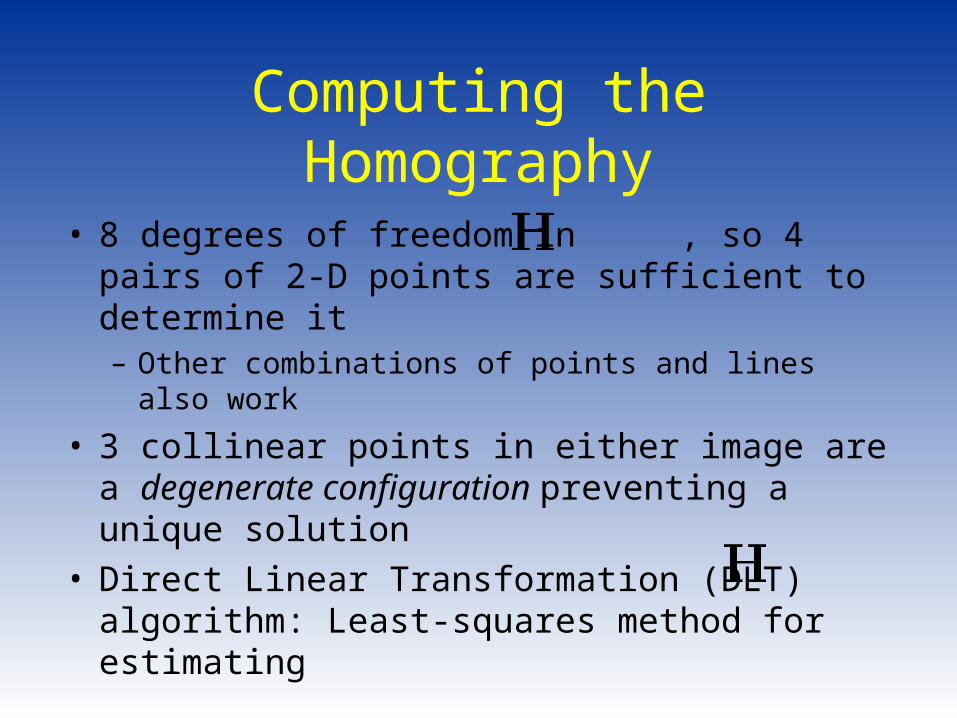
Computing the Homography

• 8 degrees of freedom in , so 4 pairs of 2-D points are sufficient to determine it– Other combinations of points and lines also

work

• 3 collinear points in either image are a degenerate configuration preventing a unique solution

• Direct Linear Transformation (DLT) algorithm: Least-squares method for estimating

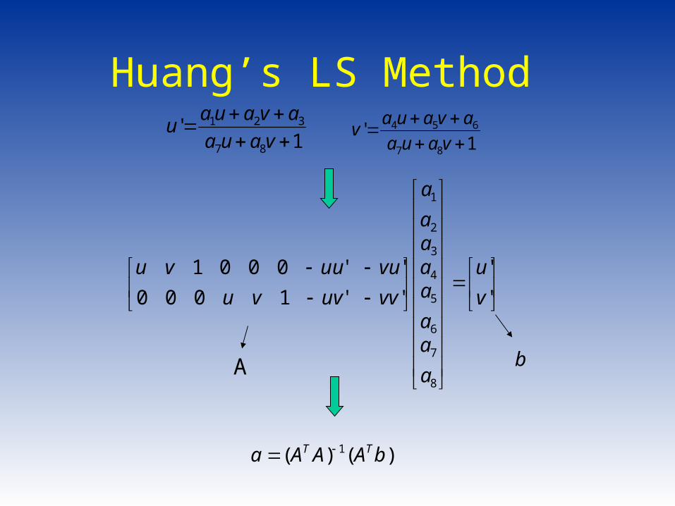
Huang’s LS Method

1'

87

654

vaua

avauav

1'

87

321

vaua

avauau

'

'

''1000

''0001

8

7

6

5

4

3

2

1

v

u

a

aa

aaaa

a

vvuvvu

vuuuvu

)()( 1 bAAAa TT

A b

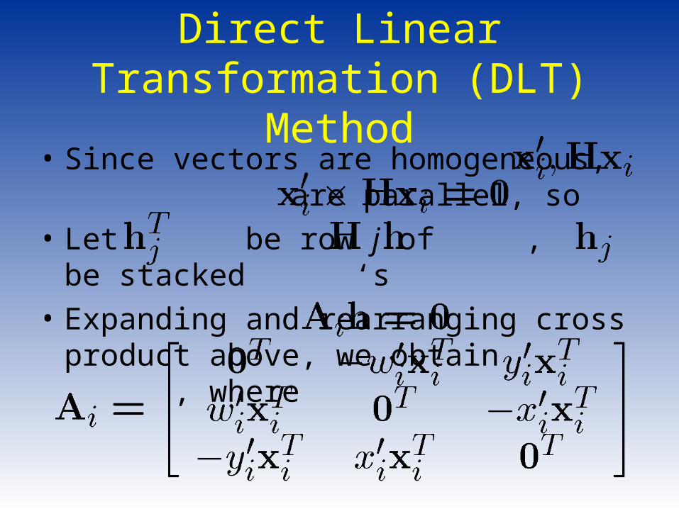
Direct Linear Transformation (DLT)

Method• Since vectors are homogeneous,

are parallel, so • Let be row j of , be stacked

‘s • Expanding and rearranging cross

product above, we obtain , where

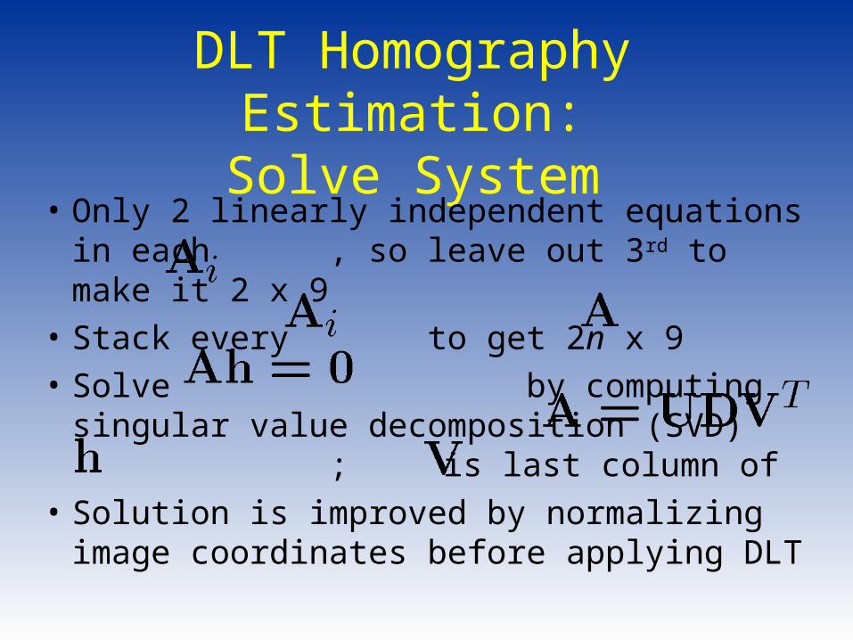
DLT Homography Estimation:

Solve System• Only 2 linearly independent equations in

each , so leave out 3rd to make it 2 x 9

• Stack every to get 2n x 9 • Solve by computing singular

value decomposition (SVD) ; is last column of

• Solution is improved by normalizing image coordinates before applying DLT

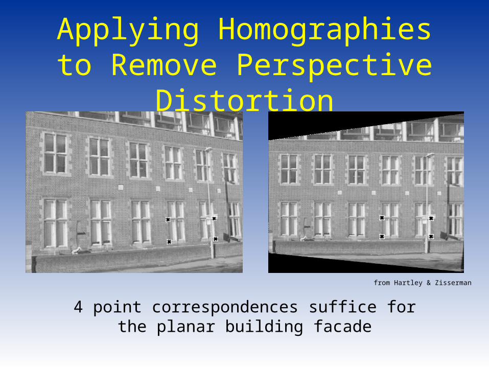
Applying Homographies to Remove Perspective

Distortion

from Hartley & Zisserman

4 point correspondences suffice forthe planar building facade

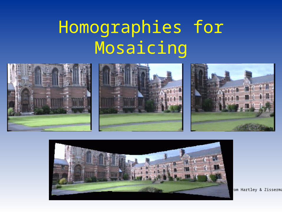
Homographies for Mosaicing

from Hartley & Zisserman