Embed Size (px)
Citation preview
Robert J. Steidl · 1
Robert J. Steidl Section IV: Curriculum Vitae
Chronology of Education
• Ph.D. Wildlife Ecology, Statistics minor, Oregon State University, September 1994 Dissertation: Human impacts on the ecology of bald eagles in interior Alaska Director: Dr. Robert G. Anthony
• M. S. Wildlife Biology, University of Massachusetts, January 1990
Thesis: Reproductive ecology of ospreys and peregrine falcons in New Jersey Director: Dr. Curtice R. Griffin
• B. S. Computer Science, Natural Resource Management minor, Rutgers University, May 1986 • Major Fields: Effects of human activities on wildlife populations; quantitative ecology; conservation biology
Chronology of Employment
• Associate Professor University of Arizona, School of Natural Resources, Wildlife Conservation and Management September 2002–present
• Assistant Professor August 1996–August 2002
Develop and maintain comprehensive teaching and research programs in applied wildlife ecology. Supervise graduate students, serve on graduate committees, and advise undergraduate students. Provide expertise on all aspects of quantitative population ecology.
• Post-Doctoral Research Associate Oregon State University, Oregon Cooperative Wildlife Research Unit
January 1995–July 1996
Research and data analysis on demography and habitat of old-forest wildlife. Co-taught one graduate-level course, supervised research assistants and graduate students.
• Graduate Research Assistant Oregon State University, Department of Fisheries & Wildlife May 1989–
December 1994
• Wildlife Biologist National Park Service, Wrangell-St. Elias National Park, Alaska April–September 1993
• Graduate Research Assistant University of Massachusetts, Department of Forestry & Wildlife
November 1986–May 1989
• Wildlife Biologist NJ Division Fish & Wildlife, Endangered & Nongame Species Program March–June 1985; April–November 1986
• Research Assistant Rutgers University, Department of Ecology
September 1985–October 1986
Robert J. Steidl · 2
Honors and Awards
2008 Outstanding M.S. Advisor, School of Natural Resources 2007 Outstanding Course Award (RNR 321), School of Natural Resources 2007 Outstanding Ph.D. Advisor, School of Natural Resources 2004 Outstanding Course Award (RNR 578), School of Natural Resources 2002 Outstanding Course Award (RNR 613), School of Natural Resources 2002 Outstanding Public Service Award, School of Natural Resources 2001 Outstanding M.S. Advisor, School of Natural Resources 1994 Outstanding Graduate Student, Oregon Chapter of The Wildlife Society 1993 Registry of Outstanding Students, Oregon State University
Service and Outreach (since 2002) • Local/State
2008 – present Advisor, Arizona Coordinated Bird Monitoring Program, Arizona Game & Fish Dept.
2006 – present Member, Science Commission, Pima County, Arizona
2003 Reviewer, Demographic analysis of the Arizona bald eagle population, Arizona Game & Fish Dept.
2002 – present Annual Speaker, “Conservation biology,” Institute of Desert Ecology, Tucson Audubon Society
2002 – 2003 Member, Kartchner Caverns Advisory Group, Arizona State Parks
2002 Speaker, “Adaptive management,” Steering Committee for Sonoran Desert Conservation
1999 – present Co-chair, Science and Technical Advisory Team, Sonoran Desert Conservation Plan, Pima County, Arizona
1998 – present Member, Ecological Monitoring Program Committee, Organ Pipe Cactus National Monument, National Park Service
• National/International
2009 Workshop Coordinator, Developing a national strategy for monitoring hummingbirds, Cooper Ornithological Society Annual Meeting
2008 Member, Scientific monitoring committee for the U.S.-Mexico border fence, U.S.G.S.
2008 Reviewer, Final recovery plan for the Northern Spotted Owl, Society for Conservation Biology
2007 – present Reviewer, Promotion and Tenure (two reviews: Texas A&M, Oregon State)
2007 Reviewer, Monitoring strategy for San Diego’s multi-species conservation plan, U.S. Fish & Wildlife Service
2007 Reviewer, Draft recovery plan for the Northern Spotted Owl, American Ornithologists Union
2007 Member, Program Committee–Workshop Chair, The Wildlife Society Annual Meeting
2006 – present Member, Desert Tortoise Scientific Advisory Committee, U.S. Fish & Wildlife Service
2006 Advisor, Establishing monitoring strategies for the Sonoran Desert Network, National Park Service
2006 Advisor, Establishing monitoring strategies for the Northeast Coastal and Barrier Network, National Park Service

Robert J. Steidl · 3
2005 Advisor, Monitoring strategy for peregrine falcons on the Colville River, Alaska, U.S. Fish & Wildlife Service and National Park Service
2005 Member, Program Committee–Contributed Papers and Session Chair, The Wildlife Society Annual Meeting
2004 – present Associate Editor, Journal of Wildlife Management
2003 – present Member, Mount Graham Red Squirrel Recovery Team, U.S. Fish & Wildlife Service
2003 Reviewer, Science related to the endangered Florida panther, U.S. Fish & Wildlife Service
2003 Session Chair, The Wildlife Society Annual Meeting
2002 Advisor, National monitoring strategy for peregrine falcons, U.S. Fish & Wildlife Service
2000 – present Reviewer, portions of scholarly books
• Heiberger and Holland, Statistical analysis and data display, Springer-Verlag • Mills, Conservation of wildlife populations, Blackwell • Shenk and Franklin, Modeling in natural resource management, Island Press • Ricklefs, Economy of nature, 5th edition, Freeman • Boitani and Fuller, Research techniques in animal ecology, Columbia
1999 – 2005 Advisor and Analyst, Best-management practices for trapping furbearers, International Association of Fish & Wildlife Agencies
1996 – present Reviewer, >75 manuscripts for scholarly journals, including American Midland Naturalist, Behavioral Ecology and Sociobiology, Biological Conservation, Condor, Conservation Biology, Ecology, Ecological Applications, Ethology, Forest Science, Journal of Wildlife Management, Raptor Research, Southwestern Naturalist, Wildlife Society Bulletin.
• Departmental
2006 Chair, Awards Committee
2004 Member, Director’s Review Committee
2002 – present Member, Faculty Search Committees (4)
2002 – present Member, Curriculum and Instruction Committee
2002 – present Member, Computer Resources Committee
2002 Chair, Seminar Committee
• College
2005 – present Member, Website Communication and Management Team
1999 – 2004 Member, Distributed Learning Team
1999 – present Reviewer, Agricultural Experiment Station Proposals (7)
• University
2007 – present Member, Faculty Search Committees (2; Math, Agricultural and Biosystems Engineering)
2006 – present Member, Graduate Interdisciplinary Program in Statistics
1999 – 2005 Member, Executive Committee and Faculty Mentor, Conservation Biology Internship Program; mentored five undergraduate students during one-year internships.
Robert J. Steidl · 4
2000 – 2003 Member, University Institutional Animal Care and Use Committee
1996 – present Statistical Consulting – Provide advice to University faculty and students in the areas of research design, data analysis, and other aspects of quantitative ecology.
• Professional Society Memberships
The Wildlife Society Ecological Society of America Society for Conservation Biology
Chapters in Scholarly Books
Steidl, R. J., W. W. Shaw, and P. Fromer. 2009. A science-based approach to regional conservation planning. Pages 217-233 in The planner's guide to natural resource conservation: the science of land development beyond the metropolitan fringe. A. X. Esparza and G. R. McPherson, editors. Scholarly book; contains both new, original research and synthesis of previous research.
Shaw, W. W., R. McCaffery, and R. J. Steidl. 2009. Integrating wildlife conservation into land-use plans for rapidly
growing cities. Pages 117-131 in The planner's guide to natural resource conservation: the science of land development beyond the metropolitan fringe. A. X. Esparza and G. R. McPherson, editors. Scholarly book; contains both new, original research and synthesis of previous research.
Koprowski, J. L., and R. J. Steidl. 2009. Consequences of small populations and their impacts on Mt. Graham red
squirrels. Pages 142-152 in The Mt. Graham red squirrel and its last refuge. Sanderson, H. R. and J. L. Koprowski, editors. , University of Arizona Press.
Steidl, R. J., and L. Thomas. 2001. Power analysis and experimental design. Pages 14-36 in Design and analysis of
ecological experiments, 2nd edition. S. Scheiner and J. Gurevitch, editors. Chapman & Hall. Scholarly book; contains both new, original research and synthesis of previous research.
Anthony, R. G., R. J. Steidl, and K. McGarigal. 1995. Recreation and bald eagles in the Pacific Northwest. Pages
223-242 in Wildlife and recreationists: coexistence through management and research. R. L. Knight and K. J. Gutzwiller, editors. Island Press. Scholarly book; contains both new, original research and synthesis of previous research.
Refereed Publications
Flesch, A. D., and R. J. Steidl. In press. Importance of environmental and spatial gradients on patterns and consequences of resource selection. Ecological Applications.
Wallace, J. E. , R. J. Steidl, and D.E. Swann. In press. Habitat of lowland leopard frogs in mountain canyons of southeastern Arizona. Journal of Wildlife Management.
Steidl, R. J., and A. R. Litt. 2009. Do plant invasions change the effects of fire on animals? Fire Ecology 5(1):56-67.
Zylstra, E. R., and R. J. Steidl. 2009. Habitat use by Sonoran Desert tortoises. Journal of Wildlife Management 73(5):747-754.
Litt, A. R., and R. J. Steidl. 2009. Improving estimates of abundance by aggregating sparse capture-recapture data. Journal of Agricultural, Biological, and Environmental Statistics 14:xxx-xxx.
Robert J. Steidl · 5
Steidl, R. J. 2008. Model based inference in the life sciences: a primer on evidence by David R. Anderson. Journal of Wildlife Management 72(7):1658-1659. Book Review.
Mannan, R. W., R. J. Steidl, and C. W. Boal. 2008. Identifying habitat sinks: a case study of Cooper’s hawks in an urban environment. Urban Ecosystems 11:141–148.
Steidl, R. J. 2007. Limits of data analysis to scientific inference: reply to Sleep et al. Journal of Wildlife Management 71(7):2122-2124.
Flesch, A. D., and R. J. Steidl. 2007. Detectability and response rates of ferruginous pygmy-owls: implications for surveying and monitoring. Journal of Wildlife Management 71(3):981-990.
Hall, D., and R. J. Steidl. 2007. Movements, activity and spacing of Sonoran mud turtles (Kinosternon sonoriense) in mountain streams of Arizona. Copeia 2007(2):403-412.
Steidl, R. J. 2006. Model selection, hypothesis testing, and risks of condemning analytical tools. Journal of Wildlife Management 70(6):1497–1498.
Flesch, A. D., and R. J. Steidl. 2006. Population trends and implications for monitoring cactus ferruginous pygmy-owls in northern Mexico. Journal of Wildlife Management 70(3):867-871.
Steidl, R. J., and B. F. Powell. 2006. Assessing the effects of human activities on wildlife. The George Wright Forum 23(2):50-58.
Ober, H. K., R. J. Steidl, and V. M. Dalton. 2005. Resource and spatial-use patterns of an endangered vertebrate pollinator, the lesser long-nosed bat. Journal of Wildlife Management 69(4):1615-1622.
Ober, H. K., and R. J. Steidl. 2004. Foraging rates of Leptonycteris curasoae vary with characteristics of Agave palmeri. Southwestern Naturalist 49(1):68-74.
Swarthout, E., and R. J. Steidl. 2003. Experimental effects of hiking on Mexican spotted owls. Conservation Biology 17(1):307-315.
Powell, B. F., and R. J. Steidl. 2002. Habitat selection by riparian songbirds breeding in southern Arizona. Journal of Wildlife Management 66(4):1096-1103.
Mann, S. L., R. J. Steidl, and V. M. Dalton. 2002. Effects of cave tours on breeding cave myotis. Journal of Wildlife Management 66(3):618-624.
Halstead, L.E., L. D. Howery, G. B. Ruyle, P. R. Krausman, and R. J. Steidl. 2002. Elk and cattle forage use under a specialized grazing system. Journal of Range Management 55(4):360-366.
Swarthout, E., and R. J. Steidl. 2001. Flush responses of Mexican spotted owls to recreationists. Journal of Wildlife Management 65(2):312-317.
Steidl, R. J. 2001. Practical and statistical considerations for designing population monitoring programs. Pages 284-288 in R. Field, R. J. Warren, H. Okarma, and P. R. Sievert, editors. Wildlife, land and people: priorities for the 21st century. Proceedings of the Second International Wildlife Management Congress, The Wildlife Society, Bethesda, Maryland.
Tull, J. C., P. R. Krausmann, and R. J. Steidl. 2001. Bed-site selection by desert mule deer in southern Arizona. Southwestern Naturalist 46(3):359-362.
DeStefano, S., and R. J. Steidl. 2001. The professional biologist and advocacy: what role do we play? Human Dimensions of Wildlife 6:11-19.
Steidl, R. J., and R. G. Anthony. 2000. Experimental effects of human activity on breeding bald eagles. Ecological Applications 10(1):258-268.
Robert J. Steidl · 6
Steidl, R. J., S. DeStefano, and W. J. Matter. 2000. On increasing the quality, reliability, and rigor of wildlife science. Wildlife Society Bulletin 28(3):518-521.
Matter, W. J., and R. J. Steidl. 2000. University undergraduate curricula in wildlife: beyond 2000. Wildlife Society Bulletin 28(3):503-507.
Powell, B. F., and R. J. Steidl. 2000. Nesting habitat and reproductive success of Southwestern riparian birds. Condor 102(4):823-831.
Daw, S. K., S. DeStefano, and R. J. Steidl. 1998. Does survey method bias the description of northern goshawk nest-site structure? Journal of Wildlife Management 62(4):1378-1383.
*Steidl, R. J., K. D. Kozie, and R. G. Anthony. 1997. Reproductive success of bald eagles in interior Alaska. Journal of Wildlife Management 61(4):1313-1321.
Steidl, R. J., J. P. Hayes, and E. Schauber. 1997. Statistical power analysis in wildlife research. Journal of Wildlife Management 61(2):270-279.
Hayes, J. P., and R. J. Steidl. 1997. Statistical power analysis and amphibian population trends. Conservation Biology 11(1):273-275.
*Steidl, R. J., C. R. Griffin, T. Augspurger, D. Sparks, and L. J. Niles. 1997. Prey of peregrine falcons from the New Jersey coast and associated contaminant levels. Northeast Wildlife 52:11-19.
*Steidl, R. J., and R. G. Anthony. 1996. Responses of bald eagles to human activity during the summer in interior Alaska. Ecological Applications 6(2):482-491.
O'Neil, T. A., R. J. Steidl, W. D. Edge, and B. Csuti. 1995. Using wildlife communities to improve vegetation classification for conserving biodiversity. Conservation Biology 9(6):1482-1491.
*Steidl, R. J., C. R. Griffin, and L. J. Niles. 1991. Contaminant levels in osprey eggs and prey reflect regional differences in reproductive success. Journal of Wildlife Management 55(4):601-608.
*Steidl, R. J., and C. R. Griffin. 1991. Growth and brood reduction of mid-Atlantic coast ospreys. Auk 108(2):363-370.
*Steidl, R. J., C. R. Griffin, L. J. Niles, and K. E. Clark. 1991. Reproductive success and eggshell thinning of reestablished peregrine falcons in New Jersey. Journal of Wildlife Management 55(2):294-299.
*Steidl, R. J., C. R. Griffin, and L. J. Niles. 1991. Differential reproductive success of ospreys in New Jersey. Journal of Wildlife Management 55(2):266-272.
* Substantially based on work done as a graduate student.
Publications in Review
Litt, A. R., and R. J. Steidl. In review. Ecological effects of fire on small mammals in grasslands invaded by nonnative plants. Wildlife Monographs.
Zylstra, E. R., R. J. Steidl, and D.E. Swann. In review. Evaluating survey methods for monitoring a rare vertebrate, the Sonoran Desert tortoise. Journal of Wildlife Management.
Litt, A. R., and R. J. Steidl. In review. Insect assemblages change along a gradient of invasion by a nonnative grass. Biological Invasions.
Robert J. Steidl · 7
Scholarly Presentations (since 2002)
2009 Designing a monitoring program for desert tortoises in Arizona. Presented by Erin R. Zylstra. Annual meeting of The Wildlife Society, Monterey, CA.
2009 Plant invasions alter demographic fitness of small mammals in grasslands. Presented by A. R. Litt. Annual meeting of The Wildlife Society, Monterey, CA.
2009 Designing a monitoring program for desert tortoises in Arizona. Presented by Erin R. Zylstra. Annual meeting of the Desert Tortoise Council, Mesquite, NV. To be delivered in September.
2009 Effects of grassland restoration efforts on breeding birds in Arizona. Science on the Sonoita Plains, Elgin, AZ. Invited.
2008 Choosing parameters for large-scale monitoring programs. Presented by A. R. Litt. Annual meeting of The Wildlife Society, Miami, FL.
2008 Estimating population trends of secretive marsh birds on the Lower Colorado River. Presented by C. J. Conway. Annual meeting of the AZ/NM chapters of The Wildlife Society, Albuquerque, NM.
2008 Comparing efficiency and statistical power of strategies used to monitor Sonoran desert tortoises. Presented by Erin R. Zylstra. Current Research on Herpetofauna of the Sonoran Desert IV, Tucson, AZ.
2008 Consequences of restoring fire to ecosystems invaded by nonnative plants. Presented by A. R. Litt. Fire in the Southwest: Integrating Fire into Management of Changing Ecosystems, Association for Fire Ecology, Tucson, AZ.
2007 Conceptual foundations for establishing recovery criteria for the Desert Tortoise. Desert Tortoise Council Symposia, Las Vegas, NV. Invited.
2007 Population and demographic trends of ferruginous pygmy-owls in northern Mexico and implications for recovery in Arizona. Presented by Aaron D. Flesch, Annual meeting of The Wildlife Society, Tucson, AZ.
2007 Habitat characteristics of lowland leopard frogs in mountain canyons of southeastern Arizona. Presented by Eric Wallace, Annual meeting of The Wildlife Society, Tucson, AZ.
2007 An ecoregional approach to monitoring for multiple-species conservation plans. Annual meeting of The Wildlife Society, Tucson, AZ.
2007 Experimental effects of vegetation and soil damage on small mammals in semi-desert grasslands. Presented by Danielle O'Dell, Annual meeting of The Wildlife Society, Tucson, AZ.
2007 Changes in a small mammal community across a gradient of invasion by nonnative grass. Presented by Andrea R. Litt, Annual meeting of The Wildlife Society, Tucson, AZ.
2007 Evaluating monitoring strategies for Sonoran desert tortoises. Presented by Erin Zylstra, Annual meeting of The Wildlife Society, Tucson, AZ.
2007 Effects of nonnative plants and restoration fires on small mammals. Presented by Andrea R. Litt, Annual meeting of the AZ/NM chapters of The Wildlife Society, Albuquerque, NM. Best student paper
2007 Comparing strategies for monitoring Sonoran desert tortoises. Presented by Erin Zylstra, Desert Tortoise Council Symposia, Las Vegas, Nevada. Best student paper
2006 Occupancy estimation as a potential strategy for monitoring Sonoran Desert Tortoises. Presented by Erin Zylstra, Desert Tortoise Council Symposia, Tucson, AZ.
Robert J. Steidl · 8
2006 Restoring ecological drivers in altered ecosystems: effects on small mammal communities. Presented by Andrea R. Litt, Annual meeting of The Wildlife Society, Anchorage, AK.
2006 Evaluating anthrogenic ecosystem stressors along the U.S.-Mexico border. Presented by Danielle O'Dell, Annual meeting of the AZ/NM chapters of The Wildlife Society, Flagstaff, AZ.
2005 Effects of non-native grasses and fire on songbirds in semi-desert grasslands. Annual meeting of The Wildlife Society, Madison, WI.
2005 Generating reliable estimates of abundance with limited capture-recapture data. Presented by Andrea R. Litt, Annual meeting of The Wildlife Society, Madison, WI.
2005 Nest selection by cactus ferruginous pygmy-owls in Sonora, Mexico and implications for management and recovery. Presented by Aaron D. Flesch, Annual meeting of the AZ/NM chapters of The Wildlife Society, Gallup, NM.
2004 The science and practice of ecosystem monitoring, Biodiversity and Management of the Madrean Archipelago, Tucson, AZ. Invited.
2004 A scientific framework for choosing parameters to monitor vertebrates. Presented by Brian F. Powell, Biodversity and Management of the Madrean Archipelago, Tucson, AZ.
2003 Species richness as a basis for large-scale conservation planning, 3rd International Wildlife Management Congress, Christchurch, New Zealand.
2003 Regional planning for biodiversity: integrating conservation into comprehensive land-use planning. Presented by William W. Shaw, 3rd International Wildlife Management Congress, Christchurch, New Zealand.
2003 Restoring ecological processes in light of ecological changes. Presented by Andrea R. Litt, 3rd International Wildlife Management Congress, Christchurch, New Zealand.
2003 Maintaining biodiversity in the suburbs: the Sonoran Desert Conservation Plan. Presented by William W. Shaw, Annual meeting of The Wildlife Society, Burlington, VT. Invited.
2002 Effects of nonnative fish on aquatic communities in small streams in the southwestern U.S. Presented by David H. Hall, Annual meeting of the Ecological Society of America, Tucson, AZ.
2002 Biological basis of the Sonoran desert conservation plan. Annual meeting of the Ecological Society of America, Tucson, AZ.
2002 Effects of nonnative grasses and fire on small mammal populations and communities. Presented by Andrea R. Litt, Annual meeting of the Ecological Society of America, Tucson, AZ.
2002 Effects of nonnative grasses on small mammal populations and communities. Presented by Andrea R. Litt, Annual meeting of the AZ/NM chapters of The Wildlife Society, Safford, AZ.
2002 Distribution, abundance, and habitat of cactus ferruginous pygmy-owls in Sonora, Mexico. Presented by Aaron D. Flesch, Annual meeting of The Wildlife Society, Bismarck, ND.
2002 Avian responses to Lehmann lovegrass in grasslands of southeastern Arizona. Presented by Eric Albrecht, Annual meeting of The Wildlife Society, Bismarck, ND.
2002 Distribution and abundance of cactus ferruginous pygmy-owls in Sonora, Mexico. Presented by Aaron D. Flesch, Annual meeting of the AZ/NM chapters of The Wildlife Society, Safford, AZ. Best student paper
2002 Avian responses to Lehmann lovegrass in grasslands of southeastern Arizona. Presented by Eric Albrecht, Annual meeting of the AZ/NM chapters of The Wildlife Society, Safford, AZ.
Robert J. Steidl · 9
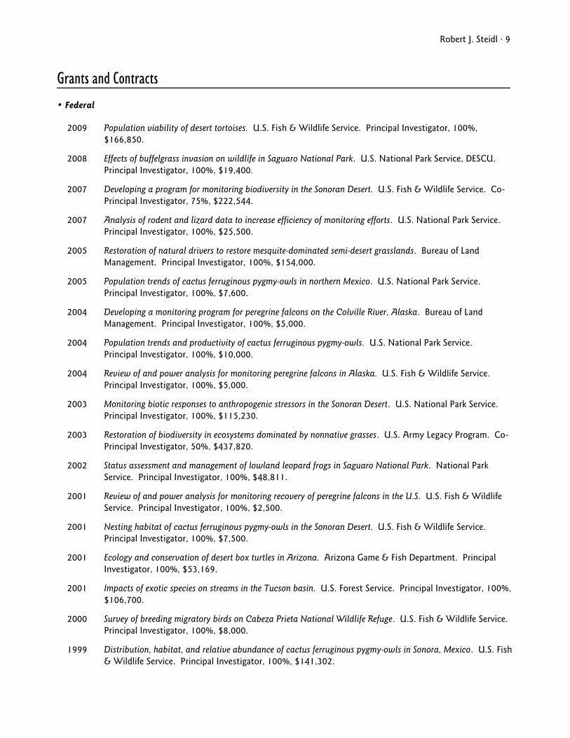
Grants and Contracts • Federal
2009 Population viability of desert tortoises. U.S. Fish & Wildlife Service. Principal Investigator, 100%, $166,850.
2008 Effects of buffelgrass invasion on wildlife in Saguaro National Park. U.S. National Park Service, DESCU. Principal Investigator, 100%, $19,400.
2007 Developing a program for monitoring biodiversity in the Sonoran Desert. U.S. Fish & Wildlife Service. Co-Principal Investigator, 75%, $222,544.
2007 Analysis of rodent and lizard data to increase efficiency of monitoring efforts. U.S. National Park Service. Principal Investigator, 100%, $25,500.
2005 Restoration of natural drivers to restore mesquite-dominated semi-desert grasslands. Bureau of Land Management. Principal Investigator, 100%, $154,000.
2005 Population trends of cactus ferruginous pygmy-owls in northern Mexico. U.S. National Park Service. Principal Investigator, 100%, $7,600.
2004 Developing a monitoring program for peregrine falcons on the Colville River, Alaska. Bureau of Land Management. Principal Investigator, 100%, $5,000.
2004 Population trends and productivity of cactus ferruginous pygmy-owls. U.S. National Park Service. Principal Investigator, 100%, $10,000.
2004 Review of and power analysis for monitoring peregrine falcons in Alaska. U.S. Fish & Wildlife Service. Principal Investigator, 100%, $5,000.
2003 Monitoring biotic responses to anthropogenic stressors in the Sonoran Desert. U.S. National Park Service. Principal Investigator, 100%, $115,230.
2003 Restoration of biodiversity in ecosystems dominated by nonnative grasses. U.S. Army Legacy Program. Co-Principal Investigator, 50%, $437,820.
2002 Status assessment and management of lowland leopard frogs in Saguaro National Park. National Park Service. Principal Investigator, 100%, $48,811.
2001 Review of and power analysis for monitoring recovery of peregrine falcons in the U.S. U.S. Fish & Wildlife Service. Principal Investigator, 100%, $2,500.
2001 Nesting habitat of cactus ferruginous pygmy-owls in the Sonoran Desert. U.S. Fish & Wildlife Service. Principal Investigator, 100%, $7,500.
2001 Ecology and conservation of desert box turtles in Arizona. Arizona Game & Fish Department. Principal Investigator, 100%, $53,169.
2001 Impacts of exotic species on streams in the Tucson basin. U.S. Forest Service. Principal Investigator, 100%, $106,700.
2000 Survey of breeding migratory birds on Cabeza Prieta National Wildlife Refuge. U.S. Fish & Wildlife Service. Principal Investigator, 100%, $8,000.
1999 Distribution, habitat, and relative abundance of cactus ferruginous pygmy-owls in Sonora, Mexico. U.S. Fish & Wildlife Service. Principal Investigator, 100%, $141,302.
Robert J. Steidl · 10
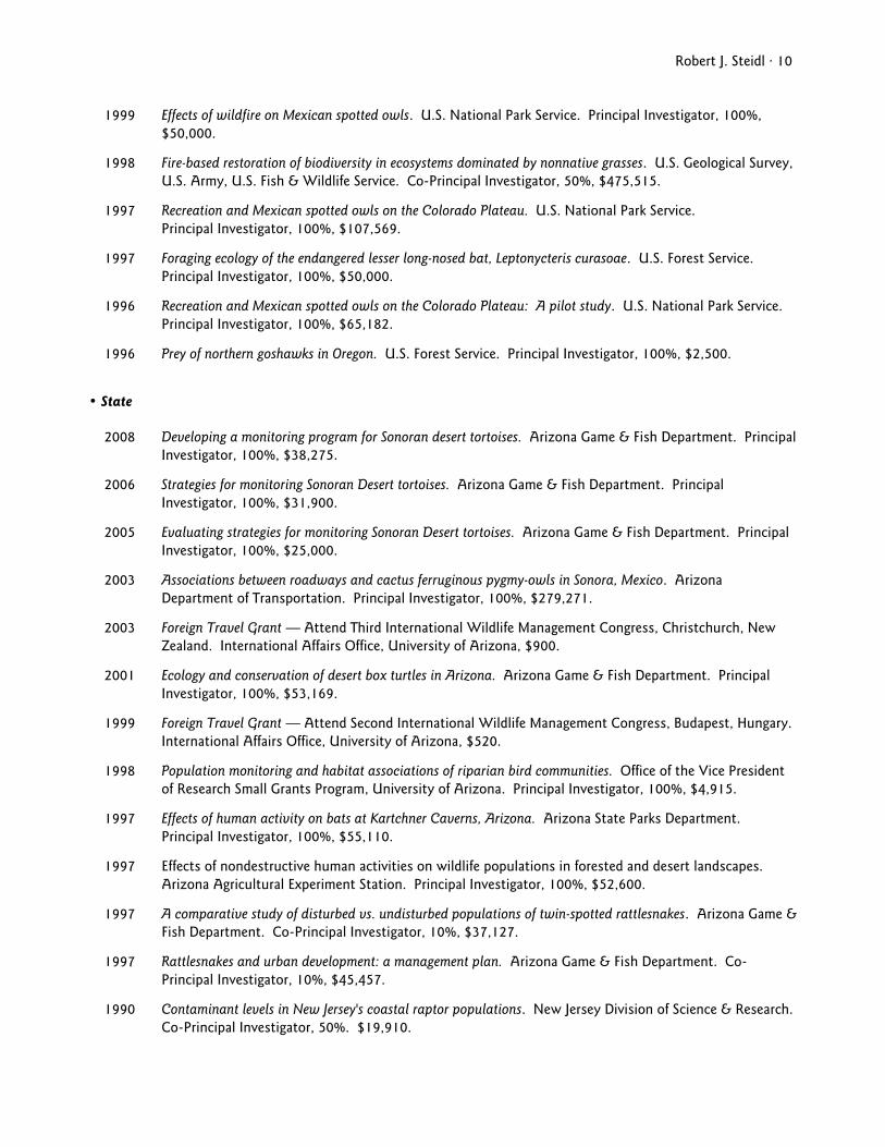
1999 Effects of wildfire on Mexican spotted owls. U.S. National Park Service. Principal Investigator, 100%, $50,000.
1998 Fire-based restoration of biodiversity in ecosystems dominated by nonnative grasses. U.S. Geological Survey, U.S. Army, U.S. Fish & Wildlife Service. Co-Principal Investigator, 50%, $475,515.
1997 Recreation and Mexican spotted owls on the Colorado Plateau. U.S. National Park Service. Principal Investigator, 100%, $107,569.
1997 Foraging ecology of the endangered lesser long-nosed bat, Leptonycteris curasoae. U.S. Forest Service. Principal Investigator, 100%, $50,000.
1996 Recreation and Mexican spotted owls on the Colorado Plateau: A pilot study. U.S. National Park Service. Principal Investigator, 100%, $65,182.
1996 Prey of northern goshawks in Oregon. U.S. Forest Service. Principal Investigator, 100%, $2,500.
• State
2008 Developing a monitoring program for Sonoran desert tortoises. Arizona Game & Fish Department. Principal Investigator, 100%, $38,275.
2006 Strategies for monitoring Sonoran Desert tortoises. Arizona Game & Fish Department. Principal Investigator, 100%, $31,900.
2005 Evaluating strategies for monitoring Sonoran Desert tortoises. Arizona Game & Fish Department. Principal Investigator, 100%, $25,000.
2003 Associations between roadways and cactus ferruginous pygmy-owls in Sonora, Mexico. Arizona Department of Transportation. Principal Investigator, 100%, $279,271.
2003 Foreign Travel Grant — Attend Third International Wildlife Management Congress, Christchurch, New Zealand. International Affairs Office, University of Arizona, $900.
2001 Ecology and conservation of desert box turtles in Arizona. Arizona Game & Fish Department. Principal Investigator, 100%, $53,169.
1999 Foreign Travel Grant — Attend Second International Wildlife Management Congress, Budapest, Hungary. International Affairs Office, University of Arizona, $520.
1998 Population monitoring and habitat associations of riparian bird communities. Office of the Vice President of Research Small Grants Program, University of Arizona. Principal Investigator, 100%, $4,915.
1997 Effects of human activity on bats at Kartchner Caverns, Arizona. Arizona State Parks Department. Principal Investigator, 100%, $55,110.
1997 Effects of nondestructive human activities on wildlife populations in forested and desert landscapes. Arizona Agricultural Experiment Station. Principal Investigator, 100%, $52,600.
1997 A comparative study of disturbed vs. undisturbed populations of twin-spotted rattlesnakes. Arizona Game & Fish Department. Co-Principal Investigator, 10%, $37,127.
1997 Rattlesnakes and urban development: a management plan. Arizona Game & Fish Department. Co-Principal Investigator, 10%, $45,457.
1990 Contaminant levels in New Jersey's coastal raptor populations. New Jersey Division of Science & Research. Co-Principal Investigator, 50%. $19,910.
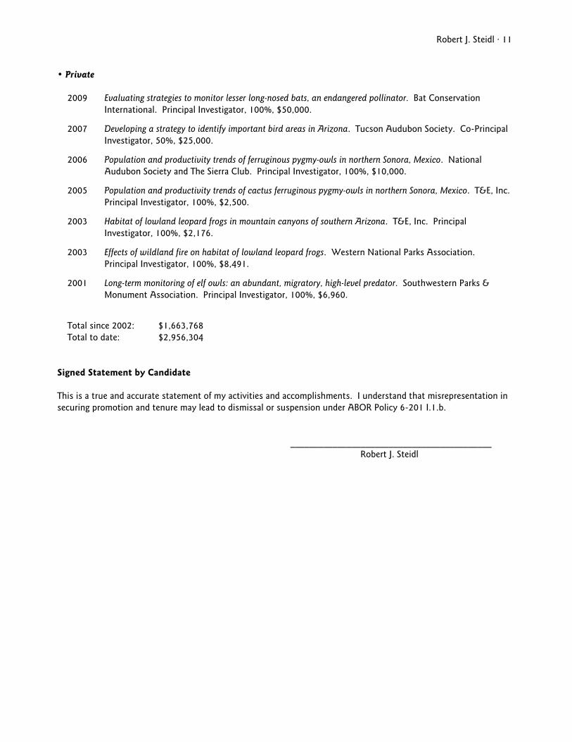
Robert J. Steidl · 11 • Private
2009 Evaluating strategies to monitor lesser long-nosed bats, an endangered pollinator. Bat Conservation International. Principal Investigator, 100%, $50,000.
2007 Developing a strategy to identify important bird areas in Arizona. Tucson Audubon Society. Co-Principal Investigator, 50%, $25,000.
2006 Population and productivity trends of ferruginous pygmy-owls in northern Sonora, Mexico. National Audubon Society and The Sierra Club. Principal Investigator, 100%, $10,000.
2005 Population and productivity trends of cactus ferruginous pygmy-owls in northern Sonora, Mexico. T&E, Inc. Principal Investigator, 100%, $2,500.
2003 Habitat of lowland leopard frogs in mountain canyons of southern Arizona. T&E, Inc. Principal Investigator, 100%, $2,176.
2003 Effects of wildland fire on habitat of lowland leopard frogs. Western National Parks Association. Principal Investigator, 100%, $8,491.
2001 Long-term monitoring of elf owls: an abundant, migratory, high-level predator. Southwestern Parks & Monument Association. Principal Investigator, 100%, $6,960.
Total since 2002: $1,663,768 Total to date: $2,956,304
Signed Statement by Candidate This is a true and accurate statement of my activities and accomplishments. I understand that misrepresentation in securing promotion and tenure may lead to dismissal or suspension under ABOR Policy 6-201 I.1.b.
___________________________________________ Robert J. Steidl
Robert J. Steidl · 12
Statement of Accomplishments & Objectives on Research, Teaching, and Service/Outreach
I serve as Associate Professor of Natural Resources in the Wildlife and Fisheries Resources Program in the School of Natural Resources, University of Arizona. I joined the faculty in fall 1996 and received tenure in fall 2002. Like all faculty, I endeavor to balance my teaching, research, and service commitments at levels commensurate with my position, which is 55% teaching, 35% research, and 10% service, and reminds me of a formative experience I had shortly after arriving at Arizona. I asked a senior faculty member how I might best balance my new responsibilities. He smiled and suggested that instead of targeting those percentages, it might be more realistic to target “100% teaching, 100% research, and 100% service.” Like most of us, I would not have it any other way. Research Research comprises 35% of my appointment. Since tenure, I have published 22 peer-reviewed papers and book chapters (43 total, 3.3/year) in a variety of national and international outlets; I have three additional papers in review. In support of my research, since tenure I have garnered $1.6 million through 23 grants and contracts ($2.9 million total, $227,500/year), principally from resource-management agencies that face challenges that align well with my research interests. Broadly, I am interested in applied ecology of vertebrates, especially issues related to conservation at population and community scales. Although I focus on applied conservation, I also seek opportunities to explore fundamental ecological questions. This union of applied and basic research has allowed me to increase the scope and breadth of my research over time, while remaining invested in solving challenges faced by resource managers. For example, in a paper to be published in Ecological Applications, we evaluated how variation in resource availability along a dramatic environmental gradient in Sonora, Mexico changed the relative importance of resources used by endangered cactus ferruginous pygmy-owls. Although our results have consequences for studies of resource selection, they also indicate that the particular resources to target for conservation and recovery can vary widely across the geographic range of a species. I divide my research into three focal areas: assessing effects of human activities on vertebrates, developing strategies to increase the efficiency and reliability of biological monitoring programs, and advancing and developing quantitative tools for ecology. Effects of human activities on vertebrates.—I am interested in understanding the effects of human activities on vertebrates and developing practical strategies to mitigate these effects. The breadth of potential human-wildlife interactions offers a wide array of research opportunities that serves to strengthen my teaching and extracurricular service activities. A recent example from this area is our effort to understand whether fire, the dominant driver in the grassland plant communities we study, affects small mammals and birds differently in areas that have been invaded by nonnative plants. We explore the conceptual importance of this novel interaction in a paper in Fire Ecology and the empirical results in papers in review by Wildlife Monographs and Biological Invasions. A thematic element of these efforts has been use of manipulative field experiments to increase their inferential strength. My work in this area has encompassed a wide range of taxa, integrated
Robert J. Steidl · 13
behavioral and demographic measures, and extended geographically across the western U.S., Mexico, and most recently into East Africa. Develop strategies to increase the efficiency and reliability of biological monitoring programs.—In the past few years, I have devoted an increasing proportion of my time to developing cohesive strategies to monitor vertebrates, with an overarching aim to increase the efficiency and reliability of large-scale monitoring programs. I began work in this area after being invited to guide development of monitoring programs for a wide range of species, communities, and ecosystems, indicating the need for scholarship and the commitment by agencies to initiate monitoring at meaningful spatial and temporal scales. Decisions about how, where, and when to allocate effort to monitor trends in resources efficiently with limited funds are complex, intellectually challenging, and provide an avenue for me to integrate my research and service contributions. These efforts are exemplified by our work to develop a program to monitor all vertebrates that inhabit the Sonoran Desert, funded by the U.S. Fish and Wildlife Service. We have formulated an explicit framework to guide development of ecoregional monitoring programs by optimizing selection from the wide range of potential target species, parameters to estimate, and sampling designs, all within a specified cost. Although we are just beginning to publish this work, I am excited by its potential to influence an important aspect of resource management over the long-term. Quantitative tools for research.—No aspect of my research reflects better my commitments to teaching and service than advancing appropriate use of quantitative tools to increase the knowledge gained through ecological data. I have written several papers and developed a series of presentations to help students and professionals better understand the increasing array of quantitative tools available, including tools for estimation, research design, and data analysis. A recent example is a paper to be published in the Journal of Agricultural, Biological, and Environmental Statistics, where we develop a heuristic strategy for estimating abundance of animal populations when capture-recapture data are sparse, as they almost always are in ecological field studies.
Teaching and Mentoring Teaching comprises 55% of my appointment, and I teach most of the quantitatively-oriented classes offered in the School. Because the subject areas that I teach progress rapidly, I revise my courses frequently and strive to improve my teaching effectiveness to better reach students with different backgrounds, skills, motivations, and intellects. I have lead the effort to increase the rigor in the School’s curricula and to keep them contemporary; these ideas are described in a pair of papers we published in the Wildlife Society Bulletin designed to help other professionals evaluating their pedagogy. My teaching centers on helping students understand the conceptual and quantitative foundations relevant to the study of applied ecology, whether the students are at the university or are professional resource managers. I aim to help students develop critical-thinking skills and to instill the ideal that science is fundamentally a creative enterprise. Despite my classes being focused on numbers, I work diligently to convey concepts that masquerade as mathematics. I think this approach serves most students well, as my course evaluations have been good, especially given the math-intensive nature of my classes, and I have received several awards for teaching.

Robert J. Steidl · 14
I involve graduate students in almost all of my research. As is apparent by authorship on the papers I’ve published, I work closely with my students, and I have graduated an average of one student per year. Typically, I secure funding for the research, then work with students to generate a set of tangible research questions, develop an efficient sampling or experimental design, analyze data, and write papers; that is, I lead them through the contemporary approach to science. Maintaining a high level of involvement in their research serves the student, me, and the research, and I hope that the high number of “outstanding thesis” or “best student presentation” awards received by my students reflects my involvement and encouragement. In terms of student credits-hours generated, I rank 4th of 31 faculty in the School who have some teaching responsibility, and I have averaged 151 credit hours per semester. I have served as major advisor for 17 graduate students, member of 37 additional graduate committees, mentored independent studies for seven undergraduate students, and supervised one post-doctoral research associate, and will recruit another this fall. Given my expertise in research design and data analysis, I contribute to research and training of many graduate students in the School even when I am not a member of their advisory committee. Service I invest considerable time in long-term, external service commitments in part because these opportunities allow me to apply my experiences to on-the-ground conservation efforts. I find serving to inform conservation decisions fulfilling and it enhances my teaching by providing tangible examples for classes. Nothing else I offer students gets their attention more than the phrase "here’s a problem we've been working on..." My most important and rewarding service activities have required knowledge of ecology and quantitative tools. Highlights have been invitations to participate in design of three ecoregional monitoring programs for the National Park Service and two national-scale monitoring programs for endangered species for the U.S. Geological Survey, and to lead a strategy to monitor the effectiveness of Multi-Species Habitat Conservation Plans on rare species by the U.S. Fish and Wildlife Service. I also have been invited to review several monitoring programs in the U.S. and in Mexico by professional societies and government agencies. I currently serve as member of the recovery teams for two rare species, and co-lead development of a comprehensive, award-winning conservation effort, the Sonoran Desert Conservation Plan (SDCP). The SDCP is a regional-scale science-driven effort designed to inform land-use planning based on conservation priorities. Development of the plan is a public process guided by a steering committee of about 80 citizens, 12 technical teams, dozens of working groups, and involvement of more than 150 scientists. I am co-chair of the central technical team, the Science Technical Advisory Team, which is responsible for identifying the network of conservation lands that will provide the foundation for all other elements in the plan. I lead development of the strategy for prioritizing lands of high biological value that form the foundation of the plan. We are currently working to establish a strategy for designing regional-scale monitoring programs that can be implemented by others seeking to enact similarly ambitious regional planning processes. Professionally, serving as Associate Editor for The Journal of Wildlife Management since 2004 has helped keep me abreast of current research in my areas of interest and has provided me the

Robert J. Steidl · 15
opportunity to offer constructive advice to authors—especially budding scientists—which has allowed me to serve the scientific community in a way that has potential impact well beyond my own research-related contributions. In this capacity, I have made decisions on more than 100 submissions. Remarkably, the University of Arizona does not have a statistics department, therefore I serve as member of an interdisciplinary team focused on providing statistical resources for research and teaching across campus. Given my role as quantitative ecologist in the School, I spend an average of 5-10% of my time consulting with students and faculty on issues related to design and analysis. Many of these interactions are with individuals associated with the School, but they sometimes include individuals in other departments in the university, local professionals, and professionals from across the country. In summary, my research, teaching, and service commitments balance on a foundation of enthusiasm for my discipline, openness to innovative ideas, and a commitment to development of others. I have sought to integrate these commitments in such a way as to help make my contribution to the university environment valuable to students, colleagues, and society.
Robert J. Steidl · 16
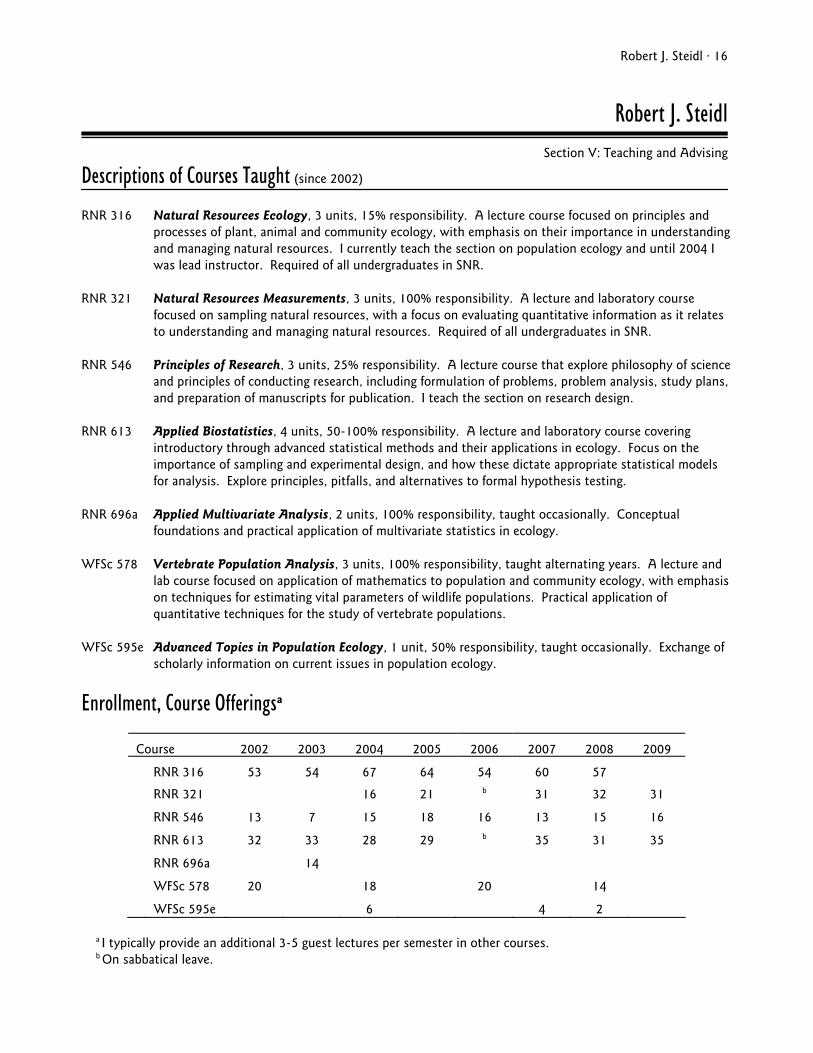
Robert J. Steidl Section V: Teaching and Advising Descriptions of Courses Taught (since 2002) RNR 316 Natural Resources Ecology, 3 units, 15% responsibility. A lecture course focused on principles and
processes of plant, animal and community ecology, with emphasis on their importance in understanding and managing natural resources. I currently teach the section on population ecology and until 2004 I was lead instructor. Required of all undergraduates in SNR.
RNR 321 Natural Resources Measurements, 3 units, 100% responsibility. A lecture and laboratory course
focused on sampling natural resources, with a focus on evaluating quantitative information as it relates to understanding and managing natural resources. Required of all undergraduates in SNR.
RNR 546 Principles of Research, 3 units, 25% responsibility. A lecture course that explore philosophy of science
and principles of conducting research, including formulation of problems, problem analysis, study plans, and preparation of manuscripts for publication. I teach the section on research design.
RNR 613 Applied Biostatistics, 4 units, 50-100% responsibility. A lecture and laboratory course covering
introductory through advanced statistical methods and their applications in ecology. Focus on the importance of sampling and experimental design, and how these dictate appropriate statistical models for analysis. Explore principles, pitfalls, and alternatives to formal hypothesis testing.
RNR 696a Applied Multivariate Analysis, 2 units, 100% responsibility, taught occasionally. Conceptual
foundations and practical application of multivariate statistics in ecology. WFSc 578 Vertebrate Population Analysis, 3 units, 100% responsibility, taught alternating years. A lecture and
lab course focused on application of mathematics to population and community ecology, with emphasis on techniques for estimating vital parameters of wildlife populations. Practical application of quantitative techniques for the study of vertebrate populations.
WFSc 595e Advanced Topics in Population Ecology, 1 unit, 50% responsibility, taught occasionally. Exchange of
scholarly information on current issues in population ecology.
Enrollment, Course Offeringsa
Course 2002 2003 2004 2005 2006 2007 2008 2009
RNR 316 53 54 67 64 54 60 57
RNR 321 16 21 b 31 32 31
RNR 546 13 7 15 18 16 13 15 16
RNR 613 32 33 28 29 b 35 31 35
RNR 696a 14
WFSc 578 20 18 20 14
WFSc 595e 6 4 2
a I typically provide an additional 3-5 guest lectures per semester in other courses. b On sabbatical leave.

Robert J. Steidl · 17
Teaching Awards (since 2002)
2007 Outstanding Course Award for RNR 321, School of Natural Resources 2004 Outstanding Course Award for RNR 578, School of Natural Resources 2002 Outstanding Course Award for RNR 613, School of Natural Resources
Individual Student Contact (since 2002) • Advising
• Major advisor to 12 graduate students who have completed degrees (1 Ph.D., 11 M.S.) • Major advisor to 3 current graduate students. • Faculty advisor to ~20 undergraduate students
• Mentoring
• Thesis advisor, University Honor’s Program, Jennifer Davison. Thesis title: Effectiveness of riparian protection on small mammal communities near developments.
• Mentor, 5 undergraduate interns in a Conservation Biology Research Internship.
Work with students to develop and implement a research project in conjunction with a co-mentor from a natural resource agency. Provide four-lecture sequence on “A short course in experimental and sampling design.”
• Graduate Committee member, 37 graduate students for whom I do not act as major advisor, 26 M.S., 11 Ph.D.
• Independent Studies
I have supervised students in 12 independent studies between 2002 and 2009, 7 undergraduate and 5 graduate. Most have focused on an aspect of quantitative ecology, population ecology, or modeling.
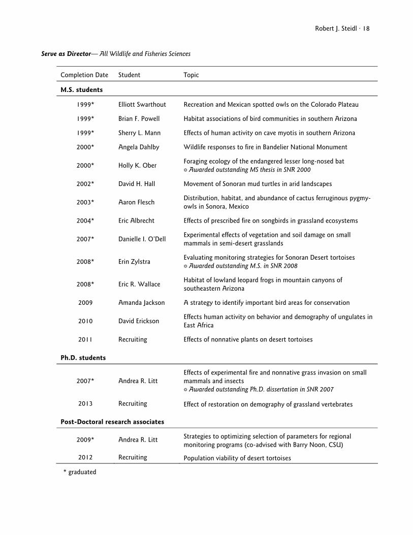
Robert J. Steidl · 18 Serve as Director— All Wildlife and Fisheries Sciences
Completion Date Student Topic
M.S. students
1999* Elliott Swarthout Recreation and Mexican spotted owls on the Colorado Plateau
1999* Brian F. Powell Habitat associations of bird communities in southern Arizona
1999* Sherry L. Mann Effects of human activity on cave myotis in southern Arizona
2000* Angela Dahlby Wildlife responses to fire in Bandelier National Monument
2000* Holly K. Ober Foraging ecology of the endangered lesser long-nosed bat ' Awarded outstanding MS thesis in SNR 2000
2002* David H. Hall Movement of Sonoran mud turtles in arid landscapes
2003* Aaron Flesch Distribution, habitat, and abundance of cactus ferruginous pygmy-owls in Sonora, Mexico
2004* Eric Albrecht Effects of prescribed fire on songbirds in grassland ecosystems
2007* Danielle I. O’Dell Experimental effects of vegetation and soil damage on small mammals in semi-desert grasslands
2008* Erin Zylstra Evaluating monitoring strategies for Sonoran Desert tortoises ' Awarded outstanding M.S. in SNR 2008
2008* Eric R. Wallace Habitat of lowland leopard frogs in mountain canyons of southeastern Arizona
2009 Amanda Jackson A strategy to identify important bird areas for conservation
2010 David Erickson Effects human activity on behavior and demography of ungulates in East Africa
2011 Recruiting Effects of nonnative plants on desert tortoises
Ph.D. students
2007* Andrea R. Litt Effects of experimental fire and nonnative grass invasion on small mammals and insects ' Awarded outstanding Ph.D. dissertation in SNR 2007
2013 Recruiting Effect of restoration on demography of grassland vertebrates
Post-Doctoral research associates
2009* Andrea R. Litt Strategies to optimizing selection of parameters for regional monitoring programs (co-advised with Barry Noon, CSU)
2012 Recruiting Population viability of desert tortoises
* graduated
Robert J. Steidl · 19
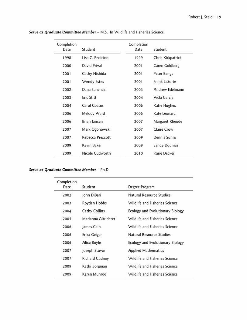
Serve as Graduate Committee Member – M.S. In Wildlife and Fisheries Science
Completion Date
Student
Completion Date
Student
1998 Lisa C. Pedicino 1999 Chris Kirkpatrick
2000 David Prival 2001 Caren Goldberg
2001 Cathy Nishida 2001 Peter Bangs
2001 Wendy Estes 2001 Frank LaSorte
2002 Dana Sanchez 2003 Andrew Edelmann
2003 Eric Stitt 2004 Vicki Garcia
2004 Carol Coates 2006 Katie Hughes
2006 Melody Ward 2006 Kate Leonard
2006 Brian Jansen 2007 Margaret Rheude
2007 Mark Ogonowski 2007 Claire Crow
2007 Rebecca Prescott 2009 Dennis Suhre
2009 Kevin Baker 2009 Sandy Doumas
2009 Nicole Cudworth 2010 Karie Decker
Serve as Graduate Committee Member – Ph.D.
Completion Date
Student
Degree Program
2002 John DiBari Natural Resource Studies
2003 Royden Hobbs Wildlife and Fisheries Science
2004 Cathy Collins Ecology and Evolutionary Biology
2005 Marianna Altrichter Wildlife and Fisheries Science
2006 James Cain Wildlife and Fisheries Science
2006 Erika Geiger Natural Resource Studies
2006 Alice Boyle Ecology and Evolutionary Biology
2007 Joseph Stover Applied Mathematics
2007 Richard Cudney Wildlife and Fisheries Science
2009 Kathi Borgman Wildlife and Fisheries Science
2009 Karen Munroe Wildlife and Fisheries Science
Robert J. Steidl · 20
Development Supporting Teaching
• Maintain web pages with course-related materials (lecture notes, assignments, data sets) for:
• RNR 321 – Natural Resources Measurements http://ag.arizona.edu/classes/rnr321.html • RNR 613 – Applied Biostatistics http://ag.arizona.edu/classes/rnr613.html • WFSc 578 – Vertebrate Population Analysis http://ag.arizona.edu/classes/wfsc578.html
Evaluation of Teaching: Preface
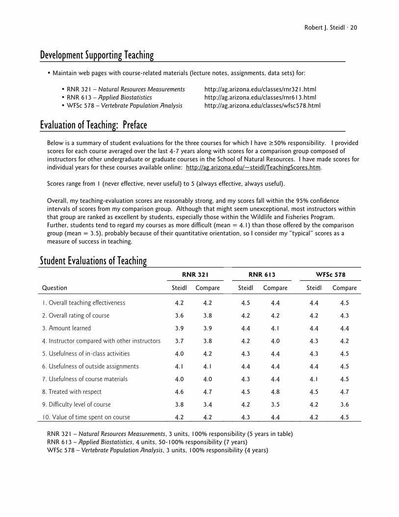
Below is a summary of student evaluations for the three courses for which I have ≥50% responsibility. I provided scores for each course averaged over the last 4-7 years along with scores for a comparison group composed of instructors for other undergraduate or graduate courses in the School of Natural Resources. I have made scores for individual years for these courses available online: http://ag.arizona.edu/~steidl/TeachingScores.htm.
Scores range from 1 (never effective, never useful) to 5 (always effective, always useful).
Overall, my teaching-evaluation scores are reasonably strong, and my scores fall within the 95% confidence intervals of scores from my comparison group. Although that might seem unexceptional, most instructors within that group are ranked as excellent by students, especially those within the Wildlife and Fisheries Program. Further, students tend to regard my courses as more difficult (mean = 4.1) than those offered by the comparison group (mean = 3.5), probably because of their quantitative orientation, so I consider my “typical” scores as a measure of success in teaching.
Student Evaluations of Teaching RNR 321 RNR 613 WFSc 578
Question Steidl Compare Steidl Compare Steidl Compare
1. Overall teaching effectiveness 4.2 4.2 4.5 4.4 4.4 4.5
2. Overall rating of course 3.6 3.8 4.2 4.2 4.2 4.3
3. Amount learned 3.9 3.9 4.4 4.1 4.4 4.4
4. Instructor compared with other instructors 3.7 3.8 4.2 4.0 4.3 4.2
5. Usefulness of in-class activities 4.0 4.2 4.3 4.4 4.3 4.5
6. Usefulness of outside assignments 4.1 4.1 4.4 4.4 4.4 4.5
7. Usefulness of course materials 4.0 4.0 4.3 4.4 4.1 4.5
8. Treated with respect 4.6 4.7 4.5 4.8 4.5 4.7
9. Difficulty level of course 3.8 3.4 4.2 3.5 4.2 3.6
10. Value of time spent on course 4.2 4.2 4.3 4.4 4.2 4.5
RNR 321 – Natural Resources Measurements, 3 units, 100% responsibility (5 years in table) RNR 613 – Applied Biostatistics, 4 units, 50-100% responsibility (7 years) WFSc 578 – Vertebrate Population Analysis, 3 units, 100% responsibility (4 years)
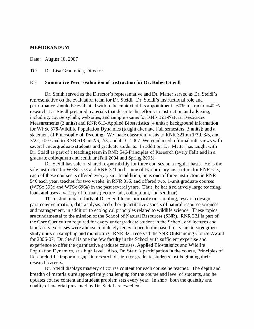
MEMORANDUM Date: August 10, 2007 TO: Dr. Lisa Graumlich, Director RE: Summative Peer Evaluation of Instruction for Dr. Robert Steidl Dr. Smith served as the Director’s representative and Dr. Matter served as Dr. Steidl’s representative on the evaluation team for Dr. Steidl. Dr. Steidl’s instructional role and performance should be evaluated within the context of his appointment - 60% instruction/40 % research. Dr. Steidl prepared materials that describe his efforts in instruction and advising, including: course syllabi, web sites, and sample exams for RNR 321-Natural Resources Measurements (3 units) and RNR 613-Applied Biostatistics (4 units); background information for WFSc 578-Wildlife Population Dynamics (taught alternate Fall semesters; 3 units); and a statement of Philosophy of Teaching. We made classroom visits to RNR 321 on 1/29, 3/5, and 3/22, 2007 and to RNR 613 on 2/6, 2/8, and 4/10, 2007. We conducted informal interviews with several undergraduate students and graduate students. In addition, Dr. Matter has taught with Dr. Steidl as part of a teaching team in RNR 546-Principles of Research (every Fall) and in a graduate colloquium and seminar (Fall 2004 and Spring 2005). Dr. Steidl has sole or shared responsibility for three courses on a regular basis. He is the sole instructor for WFSc 578 and RNR 321 and is one of two primary instructors for RNR 613; each of these courses is offered every year. In addition, he is one of three instructors in RNR 546 each year, teaches for two weeks in RNR 316, and offered two, 1-unit graduate courses (WFSc 595e and WFSc 696a) in the past several years. Thus, he has a relatively large teaching load, and uses a variety of formats (lecture, lab, colloquium, and seminar). The instructional efforts of Dr. Steidl focus primarily on sampling, research design, parameter estimation, data analysis, and other quantitative aspects of natural resource sciences and management, in addition to ecological principles related to wildlife science. These topics are fundamental to the mission of the School of Natural Resources (SNR). RNR 321 is part of the Core Curriculum required for every undergraduate student in the School, and lectures and laboratory exercises were almost completely redeveloped in the past three years to strengthen study units on sampling and monitoring. RNR 321 received the SNR Outstanding Course Award for 2006-07. Dr. Steidl is one the few faculty in the School with sufficient expertise and experience to offer the quantitative graduate courses, Applied Biostatistics and Wildlife Population Dynamics, at a high level. Also, Dr. Steidl's participation in the course, Principles of Research, fills important gaps in research design for graduate students just beginning their research careers. Dr. Steidl displays mastery of course content for each course he teaches. The depth and breadth of materials are appropriately challenging for the course and level of students, and he updates course content and student problem sets every year. In short, both the quantity and quality of material presented by Dr. Steidl are excellent.
Teaching Performance Dr. Steidl sets high academic standards for students. This is apparent in the volume and level of sophistication of material he covers. His courses are known to be among the most challenging in the School. He reinforces high expectations through his own classroom performance. He is well-prepared for each class, encourages students to ask questions and critically evaluate course materials, treats students with respect, and uses a variety of electronic and more traditional media to facilitate student learning. For example, each of Dr. Steidl's courses is supported by a web site with a detailed syllabus, notes for each class, sample examinations, data sets for exercises, homework assignments, and useful software. Dr. Steidl's teaching style is informal and entertaining. He uses an good mix of lecture and student-driven discussion, and his lectures are sufficiently broad, informative, and humorous to maintain student interest. He interjects anecdotes from personal experience and insights from his own research and recent work of other scientists when appropriate. For example, one lecture in his undergraduate measurements course included information and examples from a recent guest lecture, a recent political debate, new scientific journal articles, and Dr. Steidl's own experience in the Arctic National Wildlife Refuge. He generally arrives before the start of class and stays afterward to interact with students and answer questions. He frequently asks questions of class members to emphasize important concepts and to help monitor student understanding. During class, he is able to effectively digress to address questions or apparent lack of student comprehension. Dr. Steidl solicits feedback about his teaching and course content via mid-semester and end-of-semester evaluations. Dr. Steidl makes himself available to students during regular office hours or by appointment or drop-in meetings. Advising and Mentoring Dr. Steidl advises 10-15 undergraduate students. He is familiar with University, College, and School curriculum requirements, and he is willing to assist students with problems in career identification and professional development. He is the major advisor for 4 or 5 graduate students, and serves on advisory committees for another 15 to 17 graduate students. Graduate students recognize the high quality of mentoring they receive from Dr. Steidl. He spends a significant amount of time assisting and teaching students across the School and College of agriculture and Life Sciences with questions about research design and data analysis. Summary All evidence indicates that Dr. Steidl is a dedicated and innovative instructor. His teaching performance reflects a high level of preparation, enthusiasm, mastery of subject matter, and commitment to student learning and to improvement of his own teaching skills. He displays remarkable attention to detail in the preparation of materials for each class and he sets high academic standards. He teaches material that is highly relevant for students in SNR. Student evaluations of his courses are consistently high, despite the higher than average rigor of course content. Students indicate that Dr. Steidl is among the best teachers in the School of Natural Resources. Dr. Steidl is the type of person who is ready to make almost any moment a time for teaching and learning. Steven E. Smith William J. Matter Associate Professor Professor and Assistant Director for Academic Programs

SECTION II: SUMMARY OF CANDIDATE'S WORKLOAD ASSIGNMENT Role of the Candidate within the School’s Mission and Strategic Plan The mission of the School of Natural Resources and Environment in the College of Agriculture and Life Sciences is to serve the needs of citizens of the State of Arizona on natural resource-related issues through teaching, graduate training, extension, and research. Dr. Robert J. Steidl’s role within the School’s mission and strategic plan centers on 1) undergraduate and graduate teaching and mentoring, and 2) primary research on assessing the effects of human activities on vertebrates and developing strategies to increase the efficiency and reliability of biological monitoring programs, with emphasis on the role of quantitative ecology in research and management of wildlife focused on questions of local, regional, and global significance. Summary of Workload Assignment Dr. Steidl’s approved workload within the School of Natural Resources involves undergraduate and graduate instruction and mentoring (55%), research (35%), and intramural and extramural service and outreach activities (10%).
The University of Arizona College of Agriculture and Life Sciences
School of Natural Resources and Environment
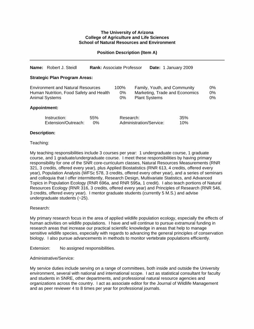
Position Description (Item A)
Name: Robert J. Steidl Rank: Associate Professor Date: 1 January 2009 Strategic Plan Program Areas: Environment and Natural Resources 100% Family, Youth, and Community 0% Human Nutrition, Food Safety and Health 0% Marketing, Trade and Economics 0% Animal Systems 0% Plant Systems 0% Appointment: Instruction: 55% Research: 35% Extension/Outreach: 0% Administration/Service: 10% Description: Teaching: My teaching responsibilities include 3 courses per year: 1 undergraduate course, 1 graduate course, and 1 graduate/undergraduate course. I meet these responsibilities by having primary responsibility for one of the SNR core-curriculum classes, Natural Resources Measurements (RNR 321, 3 credits, offered every year), plus Applied Biostatistics (RNR 613, 4 credits, offered every year), Population Analysis (WFSc 578, 3 credits, offered every other year), and a series of seminars and colloquia that I offer intermittently, Research Design, Multivariate Statistics, and Advanced Topics in Population Ecology (RNR 696a, and RNR 595a, 1 credit). I also teach portions of Natural Resources Ecology (RNR 316, 3 credits, offered every year) and Principles of Research (RNR 546, 3 credits, offered every year). I mentor graduate students (currently 5 M.S.) and advise undergraduate students (~25). Research: My primary research focus in the area of applied wildlife population ecology, especially the effects of human activities on wildlife populations. I have and will continue to pursue extramural funding in research areas that increase our practical scientific knowledge in areas that help to manage sensitive wildlife species, especially with regards to advancing the general principles of conservation biology. I also pursue advancements in methods to monitor vertebrate populations efficiently. Extension: No assigned responsibilities. Administrative/Service: My service duties include serving on a range of committees, both inside and outside the University environment, several with national and international scope. I act as statistical consultant for faculty and students in SNRE, other departments, and professional natural resource agencies and organizations across the country. I act as associate editor for the Journal of Wildlife Management and as peer reviewer 4 to 8 times per year for professional journals.

SECTION III: DEPARTMENTAL PROMOTION AND TENURE GUIDELINES Updated September, 2004 SCHOOL OF NATURAL RESOURCES and ENVIRONMENT A. Promotion and Tenure Procedures These procedures are established for the School of Natural Resources (SNR) and are intended to supplement policies and procedures outlined in the “University Handbook for Appointed Personnel (UHAP)” (http://www.arizona.edu/~uhap), and the “College of Agriculture and Life Sciences (CALS)Guidelines and Criteria for Promotion and Tenure and Promotion and Continuing Status” (http://ag.arizona.edu/dean/ptcindex.html), and CALS “Information on Promotion and Tenure/Continuing Status Issues,” (http://ag.arizona.edu/dean/cwindex.html). Should there appear to be a conflict between these School procedures and those of the College of Agriculture and Life Sciences or University Handbook, the latter will prevail. Beginning in fall, 2003, new tenure- and continuing -eligible faculty will undergo a probationary review in the third and a mandatory tenure or continuing status review in the sixth year. Faculty who have not yet had a two-year review may elect to change to the 3-year/6-year schedule. THIRD-YEAR REVIEW FOR SNR PROBATIONARY FACULTY The formal third-year review for probationary faculty will follow the guidelines and instructions issued by the Office of the Provost. These reviews will include all materials required for the promotion and tenure/continuing status dossier with the exception of outside letters. If the results of the third-year review are satisfactory but warrant an interim review prior to the sixth year, the director or dean or college committee may request an additional formalized fourth- or fifth-year review. ANNUAL REVIEWS FOR SNR PROBATIONARY FACULTY
According to UHAP 3.10.02, “annual performance reviews shall be taken into account as part of the promotion and tenure process, but such evaluations are not determinative on promotion and tenure issues. Satisfactory ratings in the annual performance reviews do not necessarily indicate successful progress toward promotion and tenure.” UHAP 4.08.02 contains similar language relevant to continuing-eligible faculty. Probationary faculty who are following the 3-year/6-year schedule must also have a special component added to their annual review to specifically assess and provide feedback on their progress toward tenure or continuing status. As part of this special annual review component, performance in teaching, research, and service (the areas of contribution necessary for tenure/continuing status), will be measured against school and college guidelines and criteria for promotion and tenure/continuing status. School criteria and performance standards are defined in sections B and C which follow. Overall progress will be assessed in the context of the faculty member’s performance to date as an indication that he or she is making progress toward meeting these criteria by the sixth year of appointment. Each year, in addition to the usual materials submitted for annual review (APROL, position description, goals and objectives), probationary faculty will submit an up-to-date curriculum vitae following the format required for the P&T/C dossier. Probationary faculty will be reviewed annually by the School Committee on Faculty Status, the Director, and the appropriate Program Chair. The Committee will provide written comments to the Director regarding the faculty member’s progress in teaching, research, and service. The Director, in consultation with the Program Chair, will also assess the faculty member’s progress and provide a written summary of the evaluation to the probationary faculty member. If progress toward tenure/continuing status as measured during the annual review is satisfactory, the Director will forward a copy of the assessment or memorandum to the Dean, but the complete set of review materials will be retained in the school. If performance in any of the three required areas (teaching, research, or service) is not satisfactory, the full review packet must be forwarded to the Dean, along with a written plan containing specific steps for improvement developed by the faculty member in consultation with the Director and

Program Chair. This plan will become part of the materials used to measure this aspect of performance in the next annual review. SCHOOL COMMITTEE ON FACULTY STATUS The following procedures govern the organization and operation of the School Committee on reviews for probationary faculty regarding Tenure/Continuing Status, Promotion, Reappointment and Non-Renewal:
(1) The Faculty Status Committee will be selected by vote of Voting Members of the School of Natural Resources Faculty. The Faculty Status Committee shall consist of three members, each serving a period of three (3) years in staggered terms with one member being designated as Chairperson. After completing a term on the Faculty Status Committee, a faculty member is not eligible for re-election to the Faculty Status Committee until one (1) full year has elapsed since the end of his or her term. In any one year, the composition of the Faculty Status Committee will have, at minimum, two (2) Full Professors. The third member can be at the Associate Professor rank or higher. Faculty in Continuing Status with comparable rank are also eligible to serve on the Faculty Status Committee. Each year, one (1) member will be elected to replace the member rotating off. To ensure that the review committee has a representative familiar with the individual's professional discipline, the individual undergoing review by the Committee will name a tenured faculty member as an ad hoc committee member to assist in his or her review. The other ad hoc member to serve on an individual's committee will be appointed by the Director after considering the compatibility of the backgrounds of the other four committee members. All members will be of higher rank than the individual being reviewed, except when a full professor is being reviewed for reappointment or tenure in which case all those voting must hold the rank of full professor. For those individuals undergoing review for promotion and/or continuing status as academic professionals, the Director will ensure that academic professional representation is included on the School Committee. In these cases of professional personnel status, standards and criteria established by the College and presented in Chapter III of the College Handbook will be utilized.
(2) All five members of the School Committee will vote on a review and the vote shall be reported.
Each faculty member or academic professional being reviewed will have the opportunity to meet with the Committee and exchange information as appropriate.
(3) The Director, in coordination with the Program Chairs, will monitor the formal review
requirements of the University and CALS and request that the Committee conduct reviews at the appropriate time. The notification to the individual to be reviewed will include guidelines for organization of materials, appropriate criteria for evaluation, the projected time schedule for completion of the review, and a copy of School, College and University procedures and/or guidelines.
(4) Each individual undergoing formal review is responsible for preparing and submitting to the
Committee the requested documentation of his or her activities within the School (vita, reprints, etc.). SNR personnel files will be available to the individual and to the Committee.
(5) Candidates for promotion and tenure/continuing status must have letters of evaluation from
professionals outside the University (at least three, but not more than six) included in their file. The candidates may suggest the names of individuals who are in a position to prepare meaningful evaluations; the Committee or Director will solicit the actual letters.
(6) The Committee will transmit its recommendation to the Director for evaluation, comments, and
subsequent action. The Committee's report will address the candidate's position or stature in the discipline area and represent a peer evaluation of scholarly and academic achievements.
(7) After receiving the Committee's report, the Director will solicit a recommendation from the
appropriate Program Chair for the purpose of obtaining additional insight and information on the candidate.

(8) The letter forwarded to the Dean by the Director will supplement information provided in the School Committee report and by the Program Chair. It will include an independent evaluation of the candidate's value and contributions as a member of the School. If not already addressed in the Committee's report, the Director will specifically identify the refereed journals and characterize the quality of these publications. The Director will notify the candidate by letter of the recommendation being forwarded to the Dean.
(9) When a recommendation regarding the granting of tenure, continuing, promotion or non-renewal
status is contemplated, a complete packet including outside letters of evaluation will be sent forward. When the Director and Program Chair contemplate recommending reappointment in rank (as opposed to recommending tenure, continuing or non-renewal) the packet minus the outside letters of recommendation will be processed through to the Dean. Upon approval of the Dean, the candidate will be informed in writing that he or she will be recommended for reappointment in rank.
B. Criteria for Promotion, Tenure, and Performance The following statements of criteria and standards for tenure, promotion and performance apply to the faculty of the School of Natural Resources. These statements clarify and extend the policies contained in the University of Arizona Handbook for Appointed Personnel, College of Agriculture and Life Sciences Guidelines and Criteria for Promotion and Tenure and Promotion and Continuing Status, and the Procedures for the School of Natural Resources Committee on Faculty Status (see above Section A ). The School Committee on Faculty Status is charged with preparing a recommendation to the Director concerning the appointment, reappointment, promotion, granting of tenure/continuing status, dismissal or nonretention of any faculty member. The School Committee will, in addition, periodically review the performance of tenured faculty. The recommendation of the Committee shall be based upon the candidate’s overall qualifications and record of performance in Instruction, Research and Scholarship and Professional Competence and Activity. Performance standards in these three areas are summarized in the following section. In evaluating a candidate's qualifications and performance against the appropriate standards, the reviewers should exercise reasonable flexibility and balance heavier commitments and responsibilities in one area against light commitments and responsibilities in another. The reviewers must judge whether the candidate is engaging in a program of work that is both sound and productive. Cases will arise in certain interdisciplinary programs within the School in which the proper work of faculty members departs markedly from established academic patters. In such cases, the reviewers must take exceptional care to apply the criteria with sufficient flexibility. However, flexibility does not entail a relaxation of high standards. For faculty members whose duties include instruction, superior intellectual attainment, as evidenced both in teaching and in either research or other creative or professional achievement, is an indispensable qualification for promotion to the rank of professor. Insistence upon this standard for the professorship is necessary for maintenance of the quality of the University as an institution dedicated to the discovery and transmission of knowledge. Promotion will be recommended upon satisfactory compliance with the performance standards of the higher rank. Tenure will normally be recommended for untenured Assistant Professors upon their promotion to Associate Professor. Untenured Associate Professors or Professors will be recommended for tenure upon a judgment that they meet the performance standards for that rank. Tenured faculty members will be evaluated periodically against the performance standards for their rank. Documentation of activities and performance will be augmented in several ways, including the annual Personnel Report, an annual peer evaluation, and a statement of an annual plan of work. A copy of the peer evaluation signed by the faculty member will be placed in the School files, along with any additional comments prepared by the faculty member concerned. The annual work plan prepared by each faculty member is normally part of the peer evaluation. It will forecast activities for the coming year and will be discussed with the Program Chair and School Director.
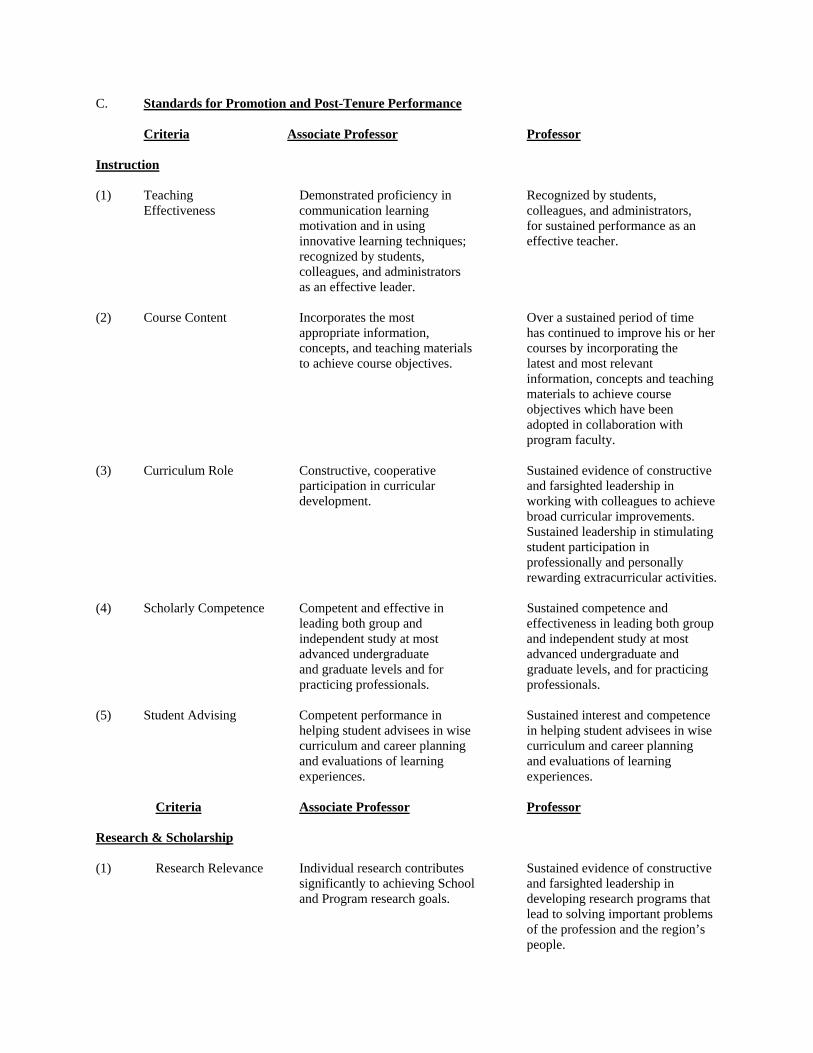
C. Standards for Promotion and Post-Tenure Performance Criteria Associate Professor Professor Instruction (1) Teaching Demonstrated proficiency in Recognized by students, Effectiveness communication learning colleagues, and administrators, motivation and in using for sustained performance as an innovative learning techniques; effective teacher. recognized by students, colleagues, and administrators as an effective leader. (2) Course Content Incorporates the most Over a sustained period of time
appropriate information, has continued to improve his or her concepts, and teaching materials courses by incorporating the
to achieve course objectives. latest and most relevant information, concepts and teaching materials to achieve course objectives which have been adopted in collaboration with program faculty.
(3) Curriculum Role Constructive, cooperative Sustained evidence of constructive participation in curricular and farsighted leadership in development. working with colleagues to achieve
broad curricular improvements. Sustained leadership in stimulating student participation in professionally and personally rewarding extracurricular activities.
(4) Scholarly Competence Competent and effective in Sustained competence and leading both group and effectiveness in leading both group independent study at most and independent study at most advanced undergraduate advanced undergraduate and and graduate levels and for graduate levels, and for practicing practicing professionals. professionals. (5) Student Advising Competent performance in Sustained interest and competence helping student advisees in wise in helping student advisees in wise curriculum and career planning curriculum and career planning
and evaluations of learning and evaluations of learning experiences. experiences.
Criteria Associate Professor Professor Research & Scholarship (1) Research Relevance Individual research contributes Sustained evidence of constructive significantly to achieving School and farsighted leadership in and Program research goals. developing research programs that
lead to solving important problems of the profession and the region’s people.
Criteria Associate Professor Professor
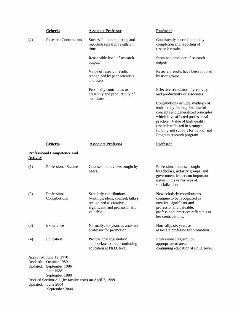
(2) Research Contribution Successful in completing and Consistently succeed in timely reporting research results on completion and reporting of time. research results. Reasonable level of research Sustained producer of research output. output. Value of research results Research results have been adopted recognized by peer scientists by user groups. and users. Personally contributes to Effective stimulator of creativity creativity and productivity of and productivity of associates. associates.
Contributions include synthesis of multi-study findings into useful concepts and generalized principles which have affected professional practice. Value of high quality research reflected in stronger funding and support for School and Program research program.
Criteria Associate Professor Professor
Professional Competence and Activity (1) Professional Stature Counsel and reviews sought by Professional counsel sought
peers. by scholars, industry groups, and government leaders on important issues in his or her area of specialization.
(2) Professional Scholarly contributions New scholarly contributions Contributions (writings, ideas, counsel, talks) continue to be recognized as recognized as creative, creative, significant and significant, and professionally professionally valuable,
valuable. professional practices reflect his or her contributions.
(3) Experience Normally, six years as assistant Normally, six years as professor for promotion. associate professor for promotion. (4) Education Professional registration Professional registration appropriate to area; continuing appropriate to area; education at Ph.D. level. continuing education at Ph.D. level. Approved: June 12, 1978 Revised: October 1980 Updated: September 1986
June 1988 September 1990
Revised Section A.1 (by faculty vote) on April 2, 1999 Updated: June 2004 September 2004
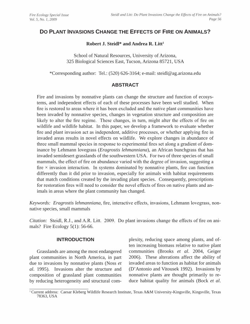
Fire Ecology Special IssueVol. 5, No. 1, 2009
Steidl and Litt: Do Plant Invasions Change the Effects of Fire on Animals?Page 56
INTRODUCTION
Grasslands are among the most endangered plant communities in North America, in part due to invasions by nonnative plants (Noss et al. 1995). Invasions alter the structure and composition of grassland plant communities by reducing heterogeneity and structural com-
plexity, reducing space among plants, and of-ten increasing biomass relative to native plant communities (Brooks et al. 2004, Geiger 2006). These alterations affect the ability of invaded areas to function as habitat for animals (D’Antonio and Vitousek 1992). Invasions by nonnative plants are thought primarily to re-duce habitat quality for animals (Bock et al.
DO PLANT INVASIONS CHANGE THE EFFECTS OF FIRE ON ANIMALS?
Robert J. Steidl* and Andrea R. Litt1
School of Natural Resources, University of Arizona,325 Biological Sciences East, Tucson, Arizona 85721, USA
*Corresponding author: Tel.: (520) 626-3164; e-mail: [email protected]
ABSTRACT
Fire and invasions by nonnative plants can change the structure and function of ecosys-tems, and independent effects of each of these processes have been well studied. When fire is restored to areas where it has been excluded and the native plant communities have been invaded by nonnative species, changes in vegetation structure and composition are likely to alter the fire regime. These changes, in turn, might alter the effects of fire on wildlife and wildlife habitat. In this paper, we develop a framework to evaluate whether fire and plant invasion act as independent, additive processes, or whether applying fire in invaded areas results in novel effects on wildlife. We explore changes in abundance of three small mammal species in response to experimental fires set along a gradient of dom-inance by Lehmann lovegrass (Eragrostis lehmanniana), an African bunchgrass that has invaded semidesert grasslands of the southwestern USA. For two of three species of small mammals, the effect of fire on abundance varied with the degree of invasion, suggesting a fire × invasion interaction. In systems dominated by nonnative plants, fire can function differently than it did prior to invasion, especially for animals with habitat requirements that match conditions created by the invading plant species. Consequently, prescriptions for restoration fires will need to consider the novel effects of fires on native plants and an-imals in areas where the plant community has changed.
Keywords: Eragrostis lehmanniana, fire, interactive effects, invasions, Lehmann lovegrass, non-native species, small mammals
Citation: Steidl, R.J., and A.R. Litt. 2009. Do plant invasions change the effects of fire on ani-mals? Fire Ecology 5(1): 56-66.
1 Current address: Caesar Kleberg Wildlife Research Institute, Texas A&M University-Kingsville, Kingsville, Texas 78363, USA
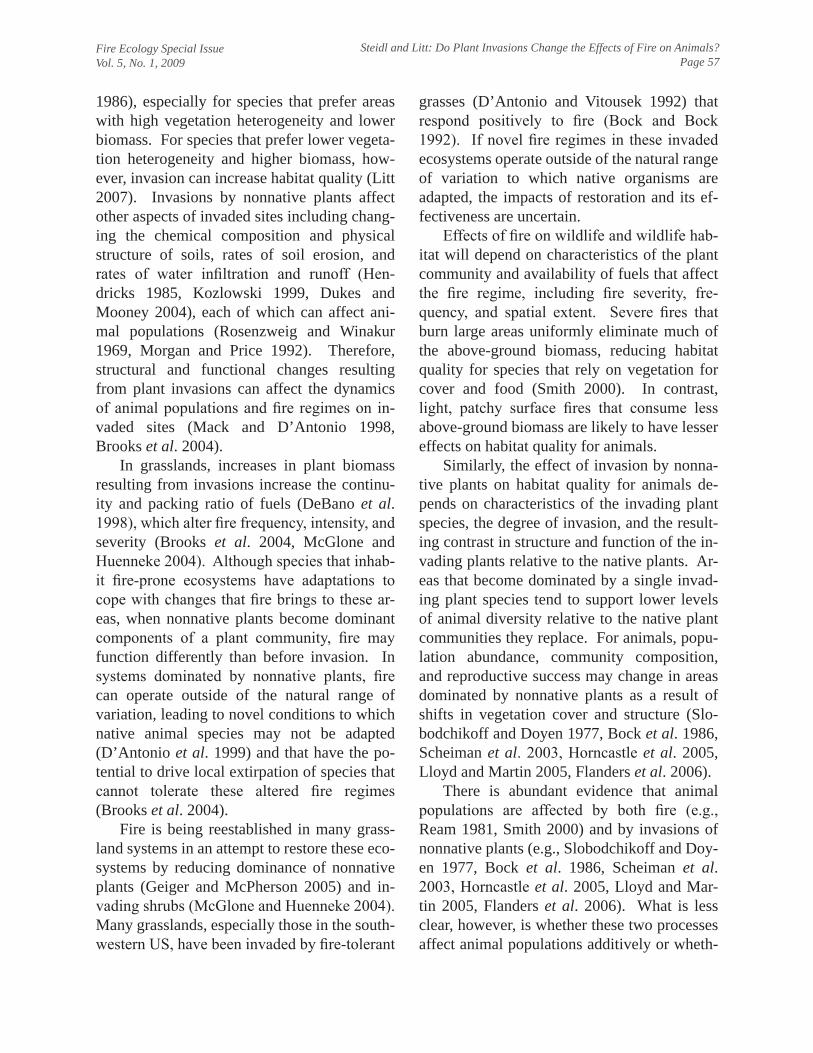
Fire Ecology Special IssueVol. 5, No. 1, 2009
Steidl and Litt: Do Plant Invasions Change the Effects of Fire on Animals?Page 57
1986), especially for species that prefer areas with high vegetation heterogeneity and lower biomass. For species that prefer lower vegeta-tion heterogeneity and higher biomass, how-ever, invasion can increase habitat quality (Litt 2007). Invasions by nonnative plants affect other aspects of invaded sites including chang-ing the chemical composition and physical structure of soils, rates of soil erosion, and rates of water infiltration and runoff (Hen-dricks 1985, Kozlowski 1999, Dukes and Mooney 2004), each of which can affect ani-mal populations (Rosenzweig and Winakur 1969, Morgan and Price 1992). Therefore, structural and functional changes resulting from plant invasions can affect the dynamics of animal populations and fire regimes on in-vaded sites (Mack and D’Antonio 1998, Brooks et al. 2004).
In grasslands, increases in plant biomass resulting from invasions increase the continu-ity and packing ratio of fuels (DeBano et al. 1998), which alter fire frequency, intensity, and severity (Brooks et al. 2004, McGlone and Huenneke 2004). Although species that inhab-it fire-prone ecosystems have adaptations to cope with changes that fire brings to these ar-eas, when nonnative plants become dominant components of a plant community, fire may function differently than before invasion. In systems dominated by nonnative plants, fire can operate outside of the natural range of variation, leading to novel conditions to which native animal species may not be adapted (D’Antonio et al. 1999) and that have the po-tential to drive local extirpation of species that cannot tolerate these altered fire regimes (Brooks et al. 2004).
Fire is being reestablished in many grass-land systems in an attempt to restore these eco-systems by reducing dominance of nonnative plants (Geiger and McPherson 2005) and in-vading shrubs (McGlone and Huenneke 2004). Many grasslands, especially those in the south-western US, have been invaded by fire-tolerant
grasses (D’Antonio and Vitousek 1992) that respond positively to fire (Bock and Bock 1992). If novel fire regimes in these invaded ecosystems operate outside of the natural range of variation to which native organisms are adapted, the impacts of restoration and its ef-fectiveness are uncertain.
Effects of fire on wildlife and wildlife hab-itat will depend on characteristics of the plant community and availability of fuels that affect the fire regime, including fire severity, fre-quency, and spatial extent. Severe fires that burn large areas uniformly eliminate much of the above-ground biomass, reducing habitat quality for species that rely on vegetation for cover and food (Smith 2000). In contrast, light, patchy surface fires that consume less above-ground biomass are likely to have lesser effects on habitat quality for animals.
Similarly, the effect of invasion by nonna-tive plants on habitat quality for animals de-pends on characteristics of the invading plant species, the degree of invasion, and the result-ing contrast in structure and function of the in-vading plants relative to the native plants. Ar-eas that become dominated by a single invad-ing plant species tend to support lower levels of animal diversity relative to the native plant communities they replace. For animals, popu-lation abundance, community composition, and reproductive success may change in areas dominated by nonnative plants as a result of shifts in vegetation cover and structure (Slo-bodchikoff and Doyen 1977, Bock et al. 1986, Scheiman et al. 2003, Horncastle et al. 2005, Lloyd and Martin 2005, Flanders et al. 2006).
There is abundant evidence that animal populations are affected by both fire (e.g., Ream 1981, Smith 2000) and by invasions of nonnative plants (e.g., Slobodchikoff and Doy-en 1977, Bock et al. 1986, Scheiman et al. 2003, Horncastle et al. 2005, Lloyd and Mar-tin 2005, Flanders et al. 2006). What is less clear, however, is whether these two processes affect animal populations additively or wheth-
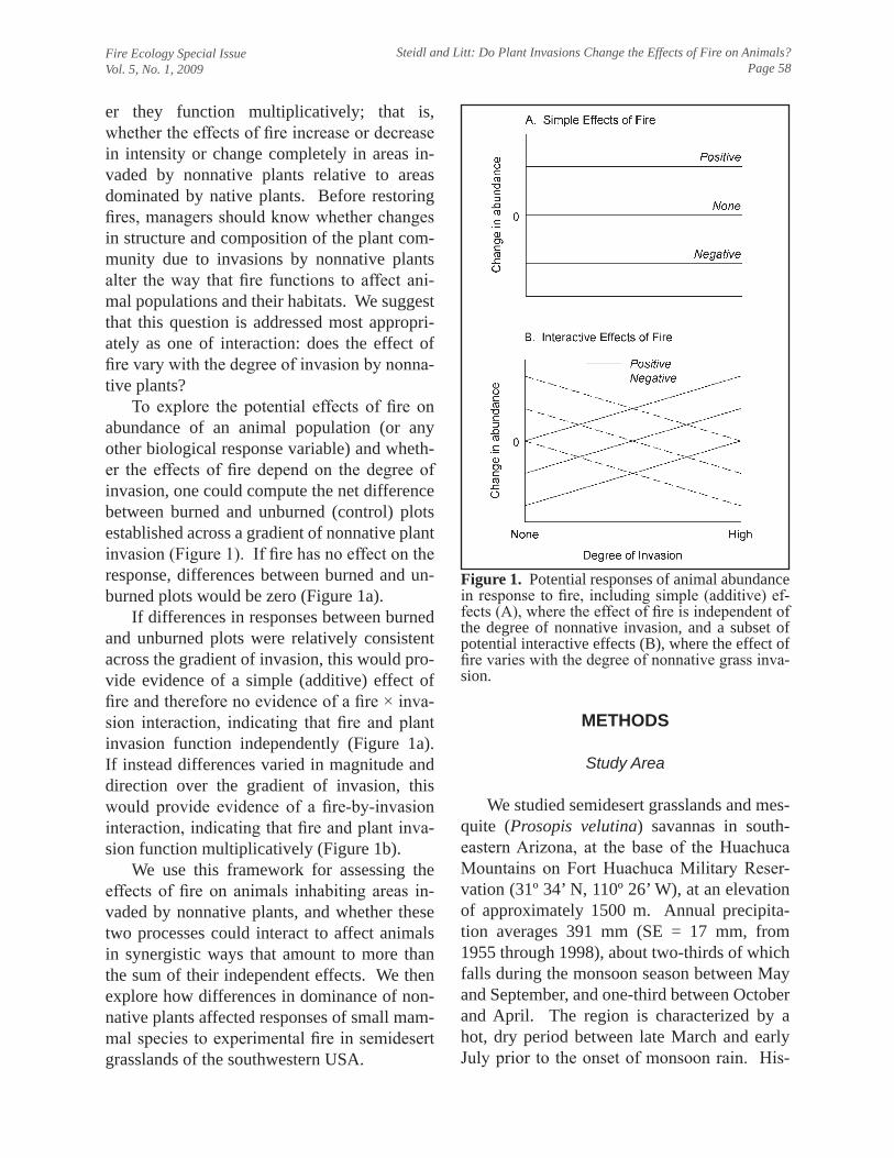
Fire Ecology Special IssueVol. 5, No. 1, 2009
Steidl and Litt: Do Plant Invasions Change the Effects of Fire on Animals?Page 58
er they function multiplicatively; that is, whether the effects of fire increase or decrease in intensity or change completely in areas in-vaded by nonnative plants relative to areas dominated by native plants. Before restoring fires, managers should know whether changes in structure and composition of the plant com-munity due to invasions by nonnative plants alter the way that fire functions to affect ani-mal populations and their habitats. We suggest that this question is addressed most appropri-ately as one of interaction: does the effect of fire vary with the degree of invasion by nonna-tive plants?
To explore the potential effects of fire on abundance of an animal population (or any other biological response variable) and wheth-er the effects of fire depend on the degree of invasion, one could compute the net difference between burned and unburned (control) plots established across a gradient of nonnative plant invasion (Figure 1). If fire has no effect on the response, differences between burned and un-burned plots would be zero (Figure 1a).
If differences in responses between burned and unburned plots were relatively consistent across the gradient of invasion, this would pro-vide evidence of a simple (additive) effect of fire and therefore no evidence of a fire × inva-sion interaction, indicating that fire and plant invasion function independently (Figure 1a). If instead differences varied in magnitude and direction over the gradient of invasion, this would provide evidence of a fire-by-invasion interaction, indicating that fire and plant inva-sion function multiplicatively (Figure 1b).
We use this framework for assessing the effects of fire on animals inhabiting areas in-vaded by nonnative plants, and whether these two processes could interact to affect animals in synergistic ways that amount to more than the sum of their independent effects. We then explore how differences in dominance of non-native plants affected responses of small mam-mal species to experimental fire in semidesert grasslands of the southwestern USA.
METHODS
Study Area
We studied semidesert grasslands and mes-quite (Prosopis velutina) savannas in south-eastern Arizona, at the base of the Huachuca Mountains on Fort Huachuca Military Reser-vation (31º 34’ N, 110º 26’ W), at an elevation of approximately 1500 m. Annual precipita-tion averages 391 mm (SE = 17 mm, from 1955 through 1998), about two-thirds of which falls during the monsoon season between May and September, and one-third between October and April. The region is characterized by a hot, dry period between late March and early July prior to the onset of monsoon rain. His-
Figure 1. Potential responses of animal abundance in response to fire, including simple (additive) ef-fects (A), where the effect of fire is independent of the degree of nonnative invasion, and a subset of potential interactive effects (B), where the effect of fire varies with the degree of nonnative grass inva-sion.
Fire Ecology Special IssueVol. 5, No. 1, 2009
Steidl and Litt: Do Plant Invasions Change the Effects of Fire on Animals?Page 59
torically, natural fires in these grasslands oc-curred about once every 10 years with their boundaries limited primarily by discontinuity of fine fuels (McPherson 1995). These fires were ignited by lightning coincident with the onset of the summer monsoon season when ambient temperatures were high and humidity and fuel moisture were low. Few livestock have grazed in this area since the late 1800s, and livestock have been excluded completely since 1950. The most recent fires on the areas we studied occurred more than nine years be-fore we initiated this study.
Our study area, like similar grasslands and savannas of the southwestern US, has been in-vaded by Lehmann lovegrass (Eragrostis lehmanniana), a nonnative perennial grass from South Africa planted in the 1930s (Crider 1945). Lehmann lovegrass produces more lit-ter and up to four times more biomass than na-tive grass species (Cable 1971, Anable et al. 1992) and has been associated with impacts on native plants and animals (Cable 1976, Bock et al. 1986, Geiger 2006). Lehmann lovegrass is well adapted to fire, with germination rates and dominance increasing after fire (Ruyle et al. 1988, Sumrall et al. 1991, Bock and Bock 1992). Common native plants included three-awn (Aristida spp.), cane blustem (Bothrio-chloa barbinodis), (Bouteloua spp.), crabgrass (Digitaria californica), plains lovegrass (Eragrostis intermedia), and panicgrass (Pani-cum spp.) (Geiger 2006).
Grasslands are especially suitable for our study because the plants are highly flammable, and the plant community is structurally simple, with less vertical structure and fewer fuel lay-ers (ground, surface, and crown) than forests. Further, rapid elimination of aboveground plant biomass after fire is usually nearly com-plete (consumption of available fuels is com-monly >90 %), which simplifies assessing the effects of fire on animals. Plant recovery in grasslands is fairly rapid (Johnson 1997, Mad-den et al. 1999), so measuring recovery after fire is efficient.
Experimental Design
We designed a manipulative randomized experiment to assess the potential for a fire × invasion interaction by measuring the effects of fire on abundance of small mammals against a gradient of invasion by nonnative plants. We established nine pairs of 1 ha plots across a gradient where Lehmann lovegrass composed 0 % to 91 % of total live biomass (mean = 44.3 %, SE = 4.9, n = 18). To maximize similarity between plots within a pair, we separated plots by 100 m to 200 m, the minimum difference we felt necessary to ensure that animal popula-tions on paired plots would be independent. We assigned the treatment (fire or control) to plots within each pair at random. Ignition of experimental fires was timed to coincide with the timing of historical lightning-ignited fires; all nine fires were completed within a four-day period in June 2001.
We used biomass (g m-2) of Lehmann lovegrass to characterize dominance of nonna-tive plants, which ranged from 0 g m-2 in areas not yet invaded up to 466 g m-2 in areas domi-nated by Lehmann lovegrass (Geiger 2006); our study plots spanned much of this gradient with biomass of Lehmann lovegrass ranging from 0 g m-2 to 333 g m-2. The difference in biomass of Lehmann lovegrass between plot pairs in the fall prior to fire averaged 48 g m-2 (95 % CI = -8 g m-2 to 102 g m-2). All vegeta-tion was clipped on 25 0.5 m2 quadrats on each plot each September from 1999 to 2003. Sam-ples were oven-dried and weighed by species for each quadrat, then averaged over all quad-rats for each plot.
Prescription for fires involved burning a 10 m to 15 m strip around the outside of the plot perimeter, setting a head fire to burn the plot, followed by spot-ignition of any unburned patches to burn as much vegetation cover as possible. At ignition, air temperature averaged 31.8 °C (range = 27.8 °C to 35.0 °C) and rela-tive humidity averaged 14 % (range = 2 % to 26 %). Immediately after each fire, we mea-
Fire Ecology Special IssueVol. 5, No. 1, 2009
Steidl and Litt: Do Plant Invasions Change the Effects of Fire on Animals?Page 60
sured completeness of fire by walking two transects established diagonally across each plot and for each step we recorded whether the immediate area was burned or unburned, from which we computed the percentage of steps that were burned.
Small Mammal Sampling
We sampled small mammals during 12 sampling periods, three periods (one year) pri-or to treatment and nine periods (three years) following treatment. After an initial sampling period in summer 2000, we sampled regularly each winter (February through March), spring (May through June), and summer (July through August), through spring 2004. Within each sampling period, all plots were sampled within a span of three to four weeks. We used an 8 × 8 grid of Sherman live traps spaced 12.5 m apart to sample small mammals on each plot. Traps were baited with wild bird seed and a mixture of peanut butter and oats, set at dusk, and checked at dawn every day for five con-secutive days. We recorded species and body measurements from all animals captured. Ani-mals were individually double-marked with a numbered ear tag and permanent felt-tipped markers, and animals were released at the site of capture. Animal-handing procedures were approved by the University of Arizona IACUC (protocols 99-121, 02-109).
We estimated abundance of Merriam’s kangaroo rat (Dipodomys merriami), northern grasshopper mouse (Onychomys leucogaster), and Arizona cotton rat (Sigmodon arizonae) on each plot for each sampling period with closed-capture Huggins models using Program MARK (version 4.3, White and Burnham 1999). We selected these species because they inhabit the range of vegetation and environ-mental conditions represented in the study area and have life-history characteristics that of-fered potential to span the range of possible re-sponses to the interaction between fire and de-
gree of nonnative plant invasion. Abundance and richness of small mammals on these 1 ha plots was high (Litt 2007); for the three spe-cies we selected, for example, abundances reached maximums of 9 to 50 individuals per species per plot. We captured 94 % of the 2822 individuals on only one plot during a sampling period, suggesting that plots were spaced sufficiently to function as independent experimental units. To increase the amount of information available for modeling detection probabilities, we aggregated data across plots for similar seasons for each species (Litt and Steidl in press). We considered candidate models for abundance estimation that included classification terms for year, fire treatment, and dominance of nonnative grass, and generated model-averaged estimates of abundance for each plot and each sampling period (Burnham and Anderson 2002).
Statistical Analyses
For each species, we quantified responses to fire as the difference in estimated abundance between pairs of burned and unburned plots using the log ratio of abundances (Törnqvist et al. 1985):
log ratio = ln (burn + 1) / ln (control + 1) = ln (burn + 1) – ln (control + 1)
This metric is valuable because it accounts for inherent differences in abundance of each species across the gradient of nonnative grass invasion, which can confound questions of in-teraction.
We evaluated models that included the ef-fects of degree of invasion, time since fire, and the interaction between the two. Because the response variable is the difference in abun-dance between burned and control pairs, the interactive effect of fire is implicit in each modeled effect. Therefore, a significant inva-sion effect indicates presence of a fire × inva-
Fire Ecology Special IssueVol. 5, No. 1, 2009
Steidl and Litt: Do Plant Invasions Change the Effects of Fire on Animals?Page 61
sion interaction. We quantified degree of inva-sion as average biomass of Lehmann lovegrass for each pair of plots for the two fall sampling periods prior to fire treatment (i.e., 1999 and 2000) and measured time since fire as the num-ber of sampling periods after treatment, and treated both variables as continuous effects in our analysis. We included pre-treatment dif-ferences in abundance of small mammals be-tween pairs of plots averaged across the three pre-fire sampling periods as a continuous co-variate to account for inherent differences in abundance among plots.
We used a generalized linear mixed-model repeated-measures approach for analysis, treat-ing plots as subjects to account for repeated measurements taken from the same plots over time (Littell et al. 2006). We considered four possible covariance structures for these models and selected the first-order autoregressive structure because it had the smallest AIC
c and
BIC values for all species.
RESULTS
Fuel load (total plant biomass) on plots prior to fire ignition averaged 313 g m-2 (SE = 36.5, range = 62 g m-2 to 437 g m-2), fuel mois-ture averaged 18 % (SE = 1.7, range = 13 to 25), and fires burned an average of 95 % (SE = 1.9, range = 84 % to 100 %) of vegetation on plots. There was no relationship between burn
completeness and biomass of Lehmann loveg-rass (t
8 = -1.5, P = 0.19), total plant biomass (t
8
= 0.8, P = 0.47), or fuel moisture (t8 = 0.3, P =
0.77), likely because burns were almost uni-formly complete.
Fire affected abundance of all three species of small mammals. For two of the three, the effect of fire on abundance varied with the de-gree of nonnative plant invasion (Table 1, Fig-ure 2). Relative to unburned controls, abun-dance of Merriam’s kangaroo rat increased af-ter fire and did so relatively consistently across the gradient of nonnative plant invasion (P = 0.87 for fire × invasion interaction). In con-trast, for both northern grasshopper mouse and Arizona cotton rat, the effects of fire on abun-dance varied with the degree of nonnative grass invasion. Abundance of northern grass-hopper mouse showed evidence of a slight positive interaction in response to fire and de-gree of nonnative plant invasion (Table 1) as both the direction and magnitude of fire effects changed across the gradient of invasion. After fire, abundance of northern grasshopper mouse decreased in areas dominated by native grass and increased in areas dominated by nonnative grass (Figure 2).
Abundance of Arizona cotton rat showed evidence of a strong negative interaction in re-sponse to fire and degree of nonnative invasion (Table 1). In contrast to northern grasshopper mouse, abundance of Arizona cotton rat almost
Dipodomys merriami Onychomys leucogaster Sigmodon arizonaeFactors F a P F P F PFire × Invasion 0.03 0.87 5.86 0.052 13.16 0.011
Fire × Time-since-fire 1.70 0.20 0.51 0.48 0.75 0.39
Fire × Invasion × Time-since-fire 1.14 0.29 1.49 0.23 3.32 0.073
Pre-treatment abundanceb 0.56 0.48 6.73 0.041 3.25 0.12
Table 1. Factors assessing differences in abundancea of small mammals between burned and control plots (n = 9 plot-pairs) in southeastern Arizona, 2000-2004. The term “invasion” represents the biomass of non-native grass on plots and “time-since-fire” represents the number of sampling periods (1-9) after fire.
a F-statistics have 70 denominator degrees of freedom for tests that include time-since-fire and 6 degrees of freedom for all other tests.
b Included as a covariate to account for inherent differences in abundance among plots.
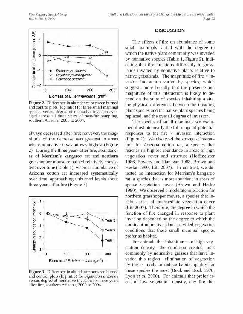
Fire Ecology Special IssueVol. 5, No. 1, 2009
Steidl and Litt: Do Plant Invasions Change the Effects of Fire on Animals?Page 62
always decreased after fire; however, the mag-nitude of the decrease was greatest in areas where nonnative invasion was highest (Figure 2). During the three years after fire, abundanc-es of Merriam’s kangaroo rat and northern grasshopper mouse remained relatively consis-tent over time (Table 1), whereas abundance of Arizona cotton rat increased systematically over time, approaching unburned levels about three years after fire (Figure 3).
DISCUSSION
The effects of fire on abundance of some small mammals varied with the degree to which the native plant community was invaded by nonnative species (Table 1, Figure 2), indi-cating that fire functions differently in grass-lands invaded by nonnative plants relative to native grasslands. The magnitude of fire × in-vasion interaction varied by species, which suggests more broadly that the presence and magnitude of this interaction is likely to de-pend on the suite of species inhabiting a site, the physical differences between the invading plant species and the native plant species being replaced, and the overall degree of invasion.
The species of small mammals we exam-ined illustrate nearly the full range of potential responses to the fire × invasion interaction (Figure 1). We observed the strongest interac-tion for Arizona cotton rat, a species that reaches its highest abundance in areas of high vegetation cover and structure (Hoffmeister 1986, Bowers and Flanagan 1988, Brown and Heske 1990, Litt 2007). In contrast, we de-tected no interaction for Merriam’s kangaroo rat, a species that is most abundant in areas of sparse vegetation cover (Brown and Heske 1990). We observed a moderate interaction for northern grasshopper mouse, a species that in-habits areas of intermediate vegetation cover (Litt 2007). Therefore, the degree to which the function of fire changed in response to plant invasion depended on the degree to which the dominant nonnative plant provided vegetation conditions that these small mammal species prefer as habitat.
For animals that inhabit areas of high veg-etation density—the condition created most commonly by nonnative grasses that have in-vaded this region—elimination of vegetation by fire is likely to reduce habitat quality for these species the most (Bock and Bock 1978, Lyon et al. 2000). For animals that prefer ar-eas of low vegetation density, any fire that
Figure 2. Difference in abundance between burned and control plots (log ratio) for three small mammal species versus degree of nonnative invasion aver-aged across all three years of post-fire sampling, southern Arizona, 2000 to 2004.
Figure 3. Difference in abundance between burned and control plots (log ratio) for Sigmodon arizonae versus degree of nonnative invasion for three years after fire, southern Arizona, 2000 to 2004.
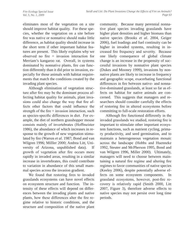
Fire Ecology Special IssueVol. 5, No. 1, 2009
Steidl and Litt: Do Plant Invasions Change the Effects of Fire on Animals?Page 63
eliminates most of the vegetation on a site should improve habitat quality. For these spe-cies, whether the vegetation on a site before fire was native or nonnative should make little difference, as habitat quality should increase in the short term if other important habitat fea-tures are present. This likely explains why we observed no fire × invasion interaction for Merriam’s kangaroo rat. Overall, in systems dominated by nonnative plants, fire can func-tion differently than it did prior to invasion, es-pecially for those animals with habitat require-ments that match the conditions created by the invading plant species.
Although elimination of vegetation struc-ture after fire may be the dominant process af-fecting habitat quality for animals, plant inva-sions could also change the way that fire af-fects other factors that could influence the strength of the fire × invasion interaction, such as species-specific differences in diet. For ex-ample, the diet of northern grasshopper mouse consists mainly of invertebrates (Hoffmeister 1986), the abundance of which increases in re-sponse to the growth of new vegetation stimu-lated by fire (Warren et al. 1987; Bond and van Wilgren 1996; Milller 2000; Andrea Litt, Uni-versity of Arizona, unpublished data). If growth of vegetation after fire occurs more rapidly in invaded areas, resulting in a similar increase in invertebrates, this could contribute to variation in abundance of this small mam-mal species across the invasion gradient.
We found that restoring fires to invaded grasslands ecosystems can have novel effects on ecosystem structure and function. The in-tensity of these effects will depend on differ-ences between the invading plants and native plants, how these differences alter the fire re-gime relative to historic conditions, and the structure and composition of the native plant
community. Because many perennial nonna-tive plant species invading grasslands have higher plant densities and higher biomass than native species (Brooks et al. 2004, Geiger 2006), fuel loadings and fuel continuity can be higher in invaded systems, resulting in in-creased fire frequency and severity. Because one likely consequence of global climate change is an increase in the propensity of suc-cessful invasions by nonnative plant species (Dukes and Mooney 1999), invasions by non-native plants are likely to increase in frequency and geographic scope, exacerbating functional differences in fire between native- and nonna-tive-dominated grasslands, at least so far as ef-fects on habitat for native animals are con-cerned. This suggests that managers and re-searchers should consider carefully the effects of restoring fire in altered ecosystems before committing to full-scale restoration efforts.
Although fire functioned differently in the invaded grasslands we studied, restoring fire is important to stimulate other important ecosys-tem functions, such as nutrient cycling, prima-ry productivity, and seed germination, and to maintain a heterogeneous vegetation mosaic across the landscape (Hobbs and Huenneke 1992, Steuter and McPherson 1995, Bond and van Wilgren 1996, Miller 2000). Ultimately, managers will need to choose between main-taining a natural fire regime and altering fire regimes to favor communities of native species (Keeley 2006), despite potentially adverse ef-fects on some ecosystem components. In grassland ecosystems, however, post-fire re-covery is relatively rapid (Smith 2000, Litt 2007, Figure 3), therefore adverse effects to native species may not persist over long time periods.
Fire Ecology Special IssueVol. 5, No. 1, 2009
Steidl and Litt: Do Plant Invasions Change the Effects of Fire on Animals?Page 64
ACkNOwLEDGEMENTS
We appreciate contributions to many aspects of this work by E.L. Geiger, G.R. McPherson, and S. Stone, as well as the help of our field assistants, too numerous to mention. We thank P. Bidegain and the dedicated crew from Fort Huachuca Fire Station No. 2 who ensured that all of the fires we proposed were set in a timely, safe, and professional manner. Our research was supported by the Department of Defense Legacy Resource Management Program and the University of Arizona Agricultural Experiment Station. Our manuscript has benefited from constructive comments provided by two anonymous reviewers.
LITERATURE CITED
Anable, M.E., M.P. McClaran, and G.B. Ruyle. 1992. Spread of introduced Lehmann lovegrass Eragrostis lehmanniana Nees in southern Arizona, USA. Biological Conservation 61: 181-188.
Bock, C.E., and J.H. Bock. 1978. Response of birds, small mammals, and vegetation to burning sacaton grasslands in southeastern Arizona. Journal of Range Management 31: 296-300.
Bock, C.E., J.H. Bock, K.L. Jepson, and J.C. Ortega. 1986. Ecological effects of planting African lovegrasses in Arizona. National Geographic Research 2: 456-463.
Bock, J.H., and C.E. Bock. 1992. Vegetation responses to wildfire in native versus exotic Arizona grassland. Journal of Vegetation Science 3: 439-446.
Bond, W.J., and B.W. van Wilgren. 1996. Fire and plants. Chapman and Hall, London, United Kingdom.
Bowers, M.A., and C.A. Flanagan. 1988. Microhabitat as a template for the organization of a desert rodent community. Pages 300-312 in: R.C. Szaro, K.E. Severson, and D.R. Patton, editors. Management of amphibians, reptiles, and small mammals in North America. USDA Forest Service General Technical Report RM-166.
Brooks, M.L., C.M. D’Antonio, D.M. Richardson, J.B. Grace, J.E. Keeley, J.M. DiTomaso, R.J. Hobbs, M. Pellant, and D. Pyke. 2004. Effects of invasive alien plants on fire regimes. Bioscience 54: 677-688.
Brown, J.H., and E.J. Heske. 1990. Control of a desert-grassland transition by a keystone rodent guild. Science 250: 1705-1707.
Burnham, K.P., and D.R. Anderson. 2002. Model selection and inference: a practical information-theoretic approach, Second edition. Springer, New York, New York, USA.
Cable, D.R. 1971. Lehmann lovegrass on the Santa Rita experimental range, 1937-1968. Journal of Range Management 24: 17-21.
Cable, D.R. 1976. Twenty years of changes in grass production following mesquite control and reseeding. Journal of Range Management 29: 286-289.
Crider, F.J. 1945. Three introduced lovegrasses for soil conservation. US Department of Agriculture Circular 730.
D’Antonio, C.M., and P.M. Vitousek. 1992. Biological invasions by exotic grasses, the grass/fire cycle, and global change. Annual Review of Ecology and Systematics 23: 63-87.
D’Antonio, C.M., T.I. Dudley, and M. Mack. 1999. Disturbance and biological invasions: direct effect and feedbacks. Pages 143-152 in: L.R. Walker, editor. Ecosystems of disturbed ground. Elsevier, Amsterdam, Netherlands.
Fire Ecology Special IssueVol. 5, No. 1, 2009
Steidl and Litt: Do Plant Invasions Change the Effects of Fire on Animals?Page 65
DeBano, L.F., D.G. Neary, and P.F. Ffolliott. 1998. Fire’s effects on ecosystems. John Wiley and Sons, New York, New York, USA.
Dukes, J.S., and H.A. Mooney. 1999. Does global change increase the success of biological invaders? Trends in Ecology and Evolution 14: 135-139.
Dukes, J.S., and H.A. Mooney. 2004. Disruption of ecosystem processes in western North America by invasive species. Revista Chilena de Historia Natural 77: 411-437.
Flanders, A.A., W.P. Kuvlesky, Jr., D.C. Ruthven, III, R.E. Zaiglin, R.L. Bingham, T.E Fulbright, F. Hernandez, and L.A. Brennan. 2006. Effects of invasive exotic grasses on south Texas rangeland breeding birds. The Auk 123: 171-182.
Geiger, E.L. 2006. The role of fire and a nonnative grass as disturbances in semi-desert grasslands of southeastern Arizona. Dissertation, University of Arizona, Tucson, USA.
Geiger, E.L., and G.R. McPherson. 2005. Response of semi-desert grasslands invaded by non-native grasses to altered disturbance regimes. Journal of Biogeography 32: 895-902.
Hendricks, D.M. 1985. Arizona soils. College of Agriculture, University of Arizona, Tucson, USA.
Hobbs, R.J., and L.F. Huenneke. 1992. Disturbance, diversity, and invasion: implications for conservation. Conservation Biology 6: 324-337.
Hoffmeister, D.F. 1986. Mammals of Arizona. University of Arizona Press, Tucson, USA.Horncastle, V.J., E.C. Hellgren, P.M. Mayer, A.C. Ganguli, D.M. Engle, and D.M. Leslie, Jr. 2005.
Implications of invasion by Juniperus virginiana on small mammals in the southern Great Plains. Journal of Mammalogy 86: 1144-1155.
Johnson, D.H. 1997. Effects of fire on bird populations in mixed-grass prairie. Pages 181-206 in: F.L. Knopf and F.B. Samson, editors. Ecology and conservation of Great Plains vertebrates. Ecological Studies Volume 125. Springer Verlag, New York, New York, USA.
Keeley, J.E. 2006. Fire management impacts on invasive plants in the western United States. Conservation Biology 20: 375-384.
Kozlowski, T.T. 1999. Soil compaction and growth of woody plants. Scandinavian Journal of Forest Research 14: 596-619.
Litt, A.R. 2007. Effects of experimental fire and nonnative grass invasion on small mammals and insects. Dissertation, University of Arizona, Tucson, USA.
Litt, A.R. and R.J. Steidl. In press. Improving estimates of abundance by aggregating sparse capture-recapture data. Journal of Agricultural, Biological, and Environmental Statistics.
Littell, R.C., G.A. Milliken, W.W. Stroup, R.D. Wolfinger, and O. Schabenberber. 2006. SAS for mixed models, second edition. SAS Press, Cary, North Carolina, USA.
Lloyd, J.D., and T.E. Martin. 2005. Reproductive success of chestnut-collared longspurs in native and exotic grassland. The Condor 107: 363-374.
Lyon, L.J., M.H. Huff, E.S. Telfer, D.S. Schreiner, and J.K. Smith. 2000. Fire effects on animal populations. Pages 25-34 in: J.K. Smith, editor. Wildland fire in ecosystems: effects of fire on fauna. USDA Forest Service General Technical Report RMRS-GTR-42-volume 1.
Mack, M.C., and C.M. D’Antonio. 1998. Impacts of biological invasions on disturbance regimes. Trends in Ecology and Evolution 13: 195-198.
Madden, E.M., A.J. Hansen, and R.K. Murphy. 1999. Influence of prescribed fire history on habitat and abundance of passerine birds in northern mixed-grass prairie. Canadian Field-Naturalist 113: 627-640.
Fire Ecology Special IssueVol. 5, No. 1, 2009
Steidl and Litt: Do Plant Invasions Change the Effects of Fire on Animals?Page 66
McPherson, G.R. 1995. The role of fire in the desert grasslands. Pages 130-151 in: M.P. McClaran and T.R. Van Devender, editors. The desert grassland. The University of Arizona Press, Tucson, USA.
McGlone, C.M., and L.F. Huenneke. 2004. The impact of a prescribed fire on introduced Lehmann lovegrass versus native vegetation in the northern Chihuahuan Desert. Journal of Arid Environments 57: 297-310.
Miller, M. 2000. Fire autecology. Pages 9-34 in: J.K. Brown and J.K. Smith, editors. Wildland fire in ecosystems: effects of fire on flora. USDA Forest Service General Technical Report RMRS-GTR-42-volume 2.
Morgan, K.R., and M.V. Price. 1992. Foraging in heteromyid rodents: the energy cost of scratch-digging. Ecology 73: 2260-2272.
Noss, R.F., E.T. LaRoe, and J.M. Scott. 1995. Endangered ecosystems of the United States: a preliminary assessment of loss and degradation. US Department of Interior, National Biological Service, Washington, D.C., USA.
Ream, C.H. 1981. The effects of fire and other disturbances on small mammals and their predators: an annotated bibliography. USDA Forest Service General Technical Report INT-106.
Rosenzweig, M.L., and J. Winakur. 1969. Population ecology of desert rodent communities: habitats and environmental complexity. Ecology 50: 558-572.
Ruyle, G.B., B.A. Roundy, and J.R. Cox. 1988. Effects of burning on germinability of Lehmann lovegrass. Journal of Range Management 41: 404-406.
Scheiman, D.M., E.K. Bollinger, and D.H. Johnson. 2003. Effects of leafy spurge infestation on grassland birds. Journal of Wildlife Management 67: 115-121.
Slobodchikoff, C.N., and J.T. Doyen. 1977. Effects of Ammophila arenaria on sand dune arthropod communities. Ecology 58: 1171-1175.
Smith, J.K., editor. 2000. Wildland fire in ecosystems: effects of fire on fauna. USDA Forest Service General Technical Report RMRS-GTR-42-volume 1.
Steuter, A.A., and G.R. McPherson. 1995. Fire as a physical stress. Pages 550-579 in: D.J. Bedunah and R.E. Sosebee, editors. Wildland plants: physiological ecology and developmental morphology. Society for Range Management, Denver, Colorado, USA.
Sumrall, L.B., B.A. Roundy, J.R. Cox, and V.K. Winkel. 1991. Influence of canopy removal by burning or clipping on emergence of Eragrostis lehmanniana seedlings. International Journal of Wildland Fire 1: 35-40.
Törnqvuist, L., P. Vartia, and Y.O. Vartia. 1985. How should relative changes be measured? The American Statistician 39: 43-46.
Vitousek, P.M., C.M. D’Antonio, L.L. Loope, and R. Westbrooks. 1996. Biological invasions as global environmental change. American Scientist 84: 468-478.
Warren, S.D., C.J. Scifres, and P.D. Teel. 1987. Response of grassland arthropods to burning: a review. Agriculture, Ecosystems, and Environment 19: 105-130.
White, G.C., and K.P. Burnham. 1999. Program MARK: survival estimation from populations of marked animals. Bird Study 46 Supplement: 120-138.
Supplemental materials for this article are available through the JABES web page athttp://www.amstat.org/publications.
1 1
2 2
3 3
4 4
5 5
6 6
7 7
8 8
9 9
10 10
11 11
12 12
13 13
14 14
15 15
16 16
17 17
18 18
19 19
20 20
21 21
22 22
23 23
24 24
25 25
26 26
27 27
28 28
29 29
30 30
31 31
32 32
33 33
34 34
35 35
36 36
37 37
38 38
39 39
40 40
41 41
42 42
43 43
44 44
Improving Estimates of Abundance byAggregating Sparse Capture-Recapture Data
Andrea R. LITT and Robert J. STEIDL
Inferences about abundance are often based on unadjusted counts of individualsobserved, in part, because of the large amount of data required to generate reliable esti-mates of abundance. Where capture-recapture data are sparse, aggregating data acrossmultiple sample elements by pooling species, locations, and sampling periods increasesthe information available for modeling detection probability, a necessary step for esti-mating abundance reliably. The process of aggregating sample elements involves bal-ancing trade-offs related to the number of aggregated elements; although larger aggre-gates increase the amount of information available for estimation, they often requiremore complex models. We describe a heuristic approach for aggregating data for stud-ies with multiple sample elements, use simulated data to evaluate the efficacy of ag-gregation, and illustrate the approach using data from a field study. Aggregating datasystematically improved reliability of model selection and increased accuracy of abun-dance estimates while still providing estimates of abundance for each original sampleunit, an important benefit necessary to maintain the design and sampling structure of astudy. Within the framework of capture-recapture sampling, aggregating data improvesestimates of abundance and increases the reliability of subsequent inferences made fromsparse data. Additional tables may be found in the online supplements.
Key Words: Abundance estimation; Data aggregation; Mark-recapture; ProgramCAPTURE; Program MARK; Population parameters.
1. INTRODUCTION
Many ecological studies seek to make inferences about changes in population size overspace, across time, or in response to experimental manipulations, and often base these in-ferences on counts of organisms that have not been adjusted for imperfect and varyingdetection probability. During a survey, many factors make it unlikely that all individualswill be detected without error. Consequently, the ability to draw reliable inferences from
Andrea R. Litt is Post-Doctoral Research Associate, School of Natural Resources, University of Arizona, 325 Bio-logical Sciences East, Tucson, AZ 85721 (E-mail: [email protected]). Robert J. Steidl is Associate Professor,School of Natural Resources, University of Arizona, 325 Biological Sciences East, Tucson, AZ 85721 (E-mail:[email protected]).
JABES asapdf v.2009/06/02 Prn:2009/06/12; 10:52 F:jabes08002.tex; (Ingrida) p. 1
1
© 2009 American Statistical Association and the International Biometric SocietyJournal of Agricultural, Biological, and Environmental Statistics, Volume 0, Number 0, Pages 1–21DOI: 10.1198/jabes.2009.08002
2 A. R. LITT AND R. J. STEIDL
1 1
2 2
3 3
4 4
5 5
6 6
7 7
8 8
9 9
10 10
11 11
12 12
13 13
14 14
15 15
16 16
17 17
18 18
19 19
20 20
21 21
22 22
23 23
24 24
25 25
26 26
27 27
28 28
29 29
30 30
31 31
32 32
33 33
34 34
35 35
36 36
37 37
38 38
39 39
40 40
41 41
42 42
43 43
44 44
counts depends on accounting for individuals not observed. The growing literature on es-timating population parameters emphasizes the fundamental need to account for imperfectdetectability to make inferences reliable (reviews in Seber 1982, 1986, 1992; Schwarz andSeber 1999).
For methods based on capture-recapture sampling, the framework and tools for mod-eling detection probability have become increasingly powerful and sophisticated. Withinthis framework, researchers ideally would generate estimates of abundance by modelingvariation in detection probability for each species, sample plot, and sampling period in astudy. Choosing an appropriate model for detection probability as the basis for generat-ing estimates of abundance, however, requires a large amount of data (Otis et al. 1978;Rosenberg, Overton, and Anthony 1995). Therefore, even when sampling effort is high,these data demands may be impossible to meet when population sizes are naturally smallor detectability is low (e.g., McKelvey and Pearson 2001; Bowden et al. 2003; MacKenzieet al. 2005).
When data are insufficient to reliably choose a model for detection probability for eachspecies, sample plot, and sampling period, studies often rely on unadjusted counts or enu-meration statistics, such as the number of unique individuals captured or the total numberof captures, to draw inferences about relative differences in abundance over space or time(McKelvey and Pearson 2001). This approach has been vigorously criticized because itassumes detection probabilities are equal among groups being compared, an assumptionthat is likely to be met only in rare circumstances (Nichols 1992; MacKenzie and Kendall2002). Further, variation in detection probability among species makes interspecific andcommunity-scale comparisons based on unadjusted counts unreliable (Nichols 1986).
At least three methods have been used commonly to overcome the high data require-ments for estimation procedures. One method is to choose a single model for detectionprobability that is then applied to all sample units (e.g., Rosenberg, Swindle, and Anthony2003). A second solution is to use traditional hypothesis tests (Skalski, Robson, and Sim-mons 1983) or equivalence tests (MacKenzie and Kendall 2002) to assess the assumptionof equal detection probability to justify the use of unadjusted counts. A third method isto estimate detection probability for a spatial or temporal subset of sample units wheredata are sufficient and use these estimates of detection probability to generate estimates ofabundance for the remaining sample units (e.g., Lynam et al. 2008). With sparse data, how-ever, there may be little information with which to rigorously evaluate the reliability of anyof these alternatives. Consequently, metrics with lower data requirements than abundanceestimation, such as occupancy or species richness, have increased in popularity (MacKen-zie et al. 2005). If study objectives dictate inferences based on abundance, however, thesemetrics may not be suitable alternatives.
When abundance is the parameter of interest and data are sparse, an additional solutionis to aggregate or pool data to increase the information available to generate estimates ofabundance that have been adjusted for detection probability. Initial approaches to aggrega-tion focused on simplifying the sampling structure within which the data were collected bypooling data across capture occasions, sites, or sampling periods in ways such that elementsof the original sample structure were lost (e.g., Hargrove and Borland 1994). Contempo-rary approaches to aggregation, such as we describe here, result in no loss of information
JABES asapdf v.2009/06/02 Prn:2009/06/12; 10:52 F:jabes08002.tex; (Ingrida) p. 2
ABUNDANCE ESTIMATES WITH AGGREGATED DATA 3
1 1
2 2
3 3
4 4
5 5
6 6
7 7
8 8
9 9
10 10
11 11
12 12
13 13
14 14
15 15
16 16
17 17
18 18
19 19
20 20
21 21
22 22
23 23
24 24
25 25
26 26
27 27
28 28
29 29
30 30
31 31
32 32
33 33
34 34
35 35
36 36
37 37
38 38
39 39
40 40
41 41
42 42
43 43
44 44
or structure and use all available data as part of the aggregation process (Boyce et al. 2001;
Bowden et al. 2003; MacKenzie et al. 2005; White 2005; Conn et al. 2006).
Although aggregating data from multiple sample units is a common practice by experts
in population analysis and some basic information is available on the process (Burnham
and Anderson 2002; MacKenzie et al. 2005; White 2005; Conn et al. 2006), our goal is to
encourage increased use of data aggregation in practice by providing a clear, synthetic de-
scription of the process by making these methods accessible to a wider range of ecologists.
Therefore, we describe a heuristic approach that uses biological and empirical information
to guide the aggregation process for studies based on capture-recapture sampling. We de-
velop a general framework for aggregation, use simulated data to examine its efficacy, and
illustrate the approach with field data.
2. OVERVIEW OF DATA AGGREGATION
Data aggregation involves assembling data from multiple sample units or “elements”
into a single dataset to increase the information available for selecting an appropriate model
for detection probability as the basis for estimating abundance. Elements to consider for
aggregation will vary by study, but might include data collected from the same sample
unit over time, from multiple sample units over space, from multiple species (MacKenzie
et al. 2005; White 2005), or even data from different studies, especially for rare species.
Aggregating data from multiple sample elements assumes that one model can be used ef-
fectively to describe the different processes driving variation in detection probability for
all elements in the aggregate. In studies where data arise from a complex set of sample
elements, the decision as to how best to aggregate data for estimation involves consider-
ing trade-offs related to the size of the aggregate. In general, larger aggregates are more
likely to combine sample elements that vary with respect to the processes that drive de-
tection probability (e.g., heterogeneity, behavior, time). More complex models and larger
datasets (i.e., more individuals) are needed to describe multiple detection processes and to
represent the more complex sampling structure of the elements combined (e.g., species,
seasons, plots) in larger aggregates. In contrast, in smaller aggregates sample elements are
likely to be more homogeneous with respect to detection processes and have simpler sam-
pling structures, requiring simpler models for detection probability and, correspondingly,
less data. Therefore, the process of aggregating data should seek to balance the benefits of
increased information available in larger aggregates with the increased complexity result-
ing from combining sample elements with disparate detection processes and more complex
sampling structures. For studies with many sample elements where several potential aggre-
gates are possible, we suggest that the process of aggregation should begin by considering
biological information as the basis for refining the set of potential aggregates, using avail-
able data to explore the complexity of processes driving detection probability in potential
aggregates, and using model-selection procedures to choose among candidate models for
detectability.
JABES asapdf v.2009/06/02 Prn:2009/06/12; 10:52 F:jabes08002.tex; (Ingrida) p. 3
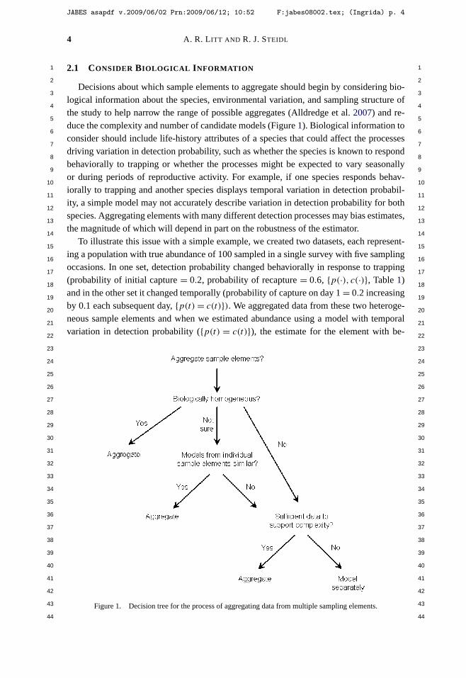
4 A. R. LITT AND R. J. STEIDL
1 1
2 2
3 3
4 4
5 5
6 6
7 7
8 8
9 9
10 10
11 11
12 12
13 13
14 14
15 15
16 16
17 17
18 18
19 19
20 20
21 21
22 22
23 23
24 24
25 25
26 26
27 27
28 28
29 29
30 30
31 31
32 32
33 33
34 34
35 35
36 36
37 37
38 38
39 39
40 40
41 41
42 42
43 43
44 44
2.1 CONSIDER BIOLOGICAL INFORMATION
Decisions about which sample elements to aggregate should begin by considering bio-logical information about the species, environmental variation, and sampling structure ofthe study to help narrow the range of possible aggregates (Alldredge et al. 2007) and re-duce the complexity and number of candidate models (Figure 1). Biological information toconsider should include life-history attributes of a species that could affect the processesdriving variation in detection probability, such as whether the species is known to respondbehaviorally to trapping or whether the processes might be expected to vary seasonallyor during periods of reproductive activity. For example, if one species responds behav-iorally to trapping and another species displays temporal variation in detection probabil-ity, a simple model may not accurately describe variation in detection probability for bothspecies. Aggregating elements with many different detection processes may bias estimates,the magnitude of which will depend in part on the robustness of the estimator.
To illustrate this issue with a simple example, we created two datasets, each represent-ing a population with true abundance of 100 sampled in a single survey with five samplingoccasions. In one set, detection probability changed behaviorally in response to trapping(probability of initial capture = 0.2, probability of recapture = 0.6, {p(·), c(·)}, Table 1)and in the other set it changed temporally (probability of capture on day 1 = 0.2 increasingby 0.1 each subsequent day, {p(t) = c(t)}). We aggregated data from these two heteroge-neous sample elements and when we estimated abundance using a model with temporalvariation in detection probability ({p(t) = c(t)}), the estimate for the element with be-
Figure 1. Decision tree for the process of aggregating data from multiple sampling elements.
JABES asapdf v.2009/06/02 Prn:2009/06/12; 10:52 F:jabes08002.tex; (Ingrida) p. 4
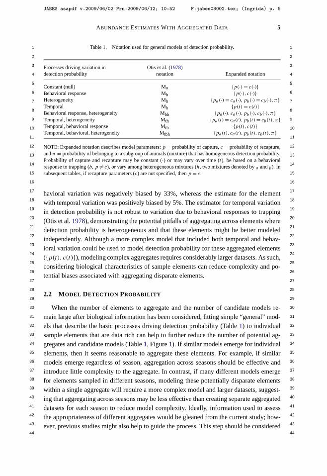
ABUNDANCE ESTIMATES WITH AGGREGATED DATA 5
1 1
2 2
3 3
4 4
5 5
6 6
7 7
8 8
9 9
10 10
11 11
12 12
13 13
14 14
15 15
16 16
17 17
18 18
19 19
20 20
21 21
22 22
23 23
24 24
25 25
26 26
27 27
28 28
29 29
30 30
31 31
32 32
33 33
34 34
35 35
36 36
37 37
38 38
39 39
40 40
41 41
42 42
43 43
44 44
Table 1. Notation used for general models of detection probability.
Processes driving variation in Otis et al. (1978)detection probability notation Expanded notation
Constant (null) Mo {p(·) = c(·)}Behavioral response Mb {p(·), c(·)}Heterogeneity Mh {pa(·) = ca(·), pb(·) = cb(·),π}Temporal Mh {p(t) = c(t)}Behavioral response, heterogeneity Mbh {pa(·), ca(·),pb(·), cb(·),π}Temporal, heterogeneity Mth {pa(t) = ca(t),pb(t) = cb(t),π}Temporal, behavioral response Mtb {p(t), c(t)}Temporal, behavioral, heterogeneity Mtbh {pa(t), ca(t),pb(t), cb(t),π}
NOTE: Expanded notation describes model parameters: p = probability of capture, c = probability of recapture,and π = probability of belonging to a subgroup of animals (mixture) that has homogeneous detection probability.Probability of capture and recapture may be constant (·) or may vary over time (t ), be based on a behavioralresponse to trapping (b, p �= c), or vary among heterogeneous mixtures (h, two mixtures denoted by a and b). Insubsequent tables, if recapture parameters (c) are not specified, then p = c.
havioral variation was negatively biased by 33%, whereas the estimate for the elementwith temporal variation was positively biased by 5%. The estimator for temporal variationin detection probability is not robust to variation due to behavioral responses to trapping(Otis et al. 1978), demonstrating the potential pitfalls of aggregating across elements wheredetection probability is heterogeneous and that these elements might be better modeledindependently. Although a more complex model that included both temporal and behav-ioral variation could be used to model detection probability for these aggregated elements({p(t), c(t)}), modeling complex aggregates requires considerably larger datasets. As such,considering biological characteristics of sample elements can reduce complexity and po-tential biases associated with aggregating disparate elements.
2.2 MODEL DETECTION PROBABILITY
When the number of elements to aggregate and the number of candidate models re-main large after biological information has been considered, fitting simple “general” mod-els that describe the basic processes driving detection probability (Table 1) to individualsample elements that are data rich can help to further reduce the number of potential ag-gregates and candidate models (Table 1, Figure 1). If similar models emerge for individualelements, then it seems reasonable to aggregate these elements. For example, if similarmodels emerge regardless of season, aggregation across seasons should be effective andintroduce little complexity to the aggregate. In contrast, if many different models emergefor elements sampled in different seasons, modeling these potentially disparate elementswithin a single aggregate will require a more complex model and larger datasets, suggest-ing that aggregating across seasons may be less effective than creating separate aggregateddatasets for each season to reduce model complexity. Ideally, information used to assessthe appropriateness of different aggregates would be gleaned from the current study; how-ever, previous studies might also help to guide the process. This step should be considered
JABES asapdf v.2009/06/02 Prn:2009/06/12; 10:52 F:jabes08002.tex; (Ingrida) p. 5
6 A. R. LITT AND R. J. STEIDL
1 1
2 2
3 3
4 4
5 5
6 6
7 7
8 8
9 9
10 10
11 11
12 12
13 13
14 14
15 15
16 16
17 17
18 18
19 19
20 20
21 21
22 22
23 23
24 24
25 25
26 26
27 27
28 28
29 29
30 30
31 31
32 32
33 33
34 34
35 35
36 36
37 37
38 38
39 39
40 40
41 41
42 42
43 43
44 44
exploratory, as these smaller datasets may not be sufficient to identify reliably complexvariation in detection processes.
After establishing aggregates, the set of candidate models that will be used to modeldetection probability for the aggregated data are developed. Starting with simple generalmodels that describe the basic processes driving detection probability (Table 1), classifica-tion variables or covariates that represent the structure of the sample elements combinedin the aggregate are incorporated into models. These “flexible” models can be createdby denoting each aggregated element as a unique “group” in the input dataset containingcapture histories, building design matrices to identify the structure of the individual sam-ple elements, and incorporating additive or multiplicative terms to constrain variables andeffectively create a wide range of related flexible models. As such, values for detectionprobability can be allowed to vary for individual elements or sets of elements in the ag-gregate. The process of starting with a general model then adding parameters to increasemodel flexibility for capture-recapture data is analogous to selecting a key function thenincorporating a series expansion within the context of distance sampling (Buckland et al.1993); that is, adding parameters increases the ability of the model to describe variationinherent in the data.
The number and complexity of flexible models can increase quickly as the number ofelements aggregated and the number of classification variables increase, which can easilyrequire hundreds of parameters. For example, fitting a model with both temporal variationand heterogeneity in detection probability for data with five capture occasions requires asmany as 11 parameters for just one sample element ({pa(t) = ca(t),pb(t) = cb(t),π}). Foran aggregate that includes data for one species from five plots sampled in three seasons,the fully multiplicative time and heterogeneity model for these 15 sample elements re-quires 165 parameters ({pa(t ∗season∗plot) = ca(t ∗season∗plot),pb(t ∗season∗plot) =cb(t ∗ season ∗ plot),π}). Thus, using biological information to refine the aggregate andcandidate model set is necessary to ensure that the number of models, the number of modelparameters, and the size of design matrices remain manageable. In addition, detecting verycomplex patterns of variation in detection processes require rich datasets (Anderson, Burn-ham, and White 1994). Once the set of candidate flexible models has been refined and fit,support for these models can be assessed within an information-theoretic framework (Fig-ure 1).
2.3 GENERATE ESTIMATES
Estimates of abundance could be generated based on the flexible model with the mostsupport (e.g., smallest AICc) or averaged across competing models to account for uncer-tainty in model selection (Burnham and Anderson 2002). Because aggregated elements areidentified uniquely as groups within the input dataset, unique estimates of abundance canbe generated for each sample element (Figure 1) as data are pooled only for the purposesof improving estimates. These element-specific estimates can be used within a hypothesis-testing framework to address questions about treatment effects because the experimentalunits and design structure for randomized experiments has been retained and traditional
JABES asapdf v.2009/06/02 Prn:2009/06/12; 10:52 F:jabes08002.tex; (Ingrida) p. 6
ABUNDANCE ESTIMATES WITH AGGREGATED DATA 7
1 1
2 2
3 3
4 4
5 5
6 6
7 7
8 8
9 9
10 10
11 11
12 12
13 13
14 14
15 15
16 16
17 17
18 18
19 19
20 20
21 21
22 22
23 23
24 24
25 25
26 26
27 27
28 28
29 29
30 30
31 31
32 32
33 33
34 34
35 35
36 36
37 37
38 38
39 39
40 40
41 41
42 42
43 43
44 44
estimates of experimental error can be used as a basis for inference. Although other ap-proaches also could be used to answer these questions, a frequentist approach offers ad-vantages within the context of randomized, replicated designs (Burnham and Anderson2002).
3. EFFICACY OF AGGREGATING
3.1 SIMULATION METHODS
We used simulations to explore consequences of aggregating data for two challengesassociated with sparse data: choosing an appropriate model for detection probability andgenerating accurate estimates. Simulated survey data were based on five trapping occa-sions, a duration common for small mammal studies (McKelvey and Pearson 2001). Wecreated aggregates that included three sample elements that could represent multiple sur-veys of the same sample unit or three sample units surveyed simultaneously, for example.
We manipulated three factors in simulations: (1) the true flexible model used to gen-erate the data, (2) overall detection probability, and (3) true abundance (N ) of the en-tire aggregate. We modeled three types of variation in detection probability to represent arange of detection processes: heterogeneity, behavioral response, and temporal variation.For simulated data with heterogeneity, we established two groups of equal size (π = 0.5),each with different detection probabilities (Appendix 1). For simulated data with a be-havioral response, we set recapture probability to be higher than the probability of initialcapture, a trap-happy response (Appendix 2). For simulated data with temporal variation,we set detection probability to be lowest on the first occasion, slightly higher and con-stant on the second through fourth sampling occasions, and highest on the fifth occasion(Appendix 3), a scenario that might reflect studies where trapping begins without a pre-baiting period. We explored different flexible models to generate data where detectionprobability among elements in the aggregate was (1) constant (e.g., {p(t) = c(t)}), (2) var-ied additively (e.g., {p(t + group) = c(t + group)}), and (3) varied multiplicatively (e.g.,{p(t ∗ group) = c(t ∗ group)}). We examined two levels of detection probability (low andhigh, Appendices 1–3) and six values of true abundance for the entire aggregate (60, 150,300, 600, 1200, or 1500 individuals), with true abundance varying among the three el-ements (each element was 1/3, 1/6, 1/2 of the total true abundance) in the aggregate.The resulting aggregate size (number of individuals captured) was a function of true abun-dance of the aggregate and detection probability. We considered all levels of factors inall combinations, yielding 126 sets of simulations, and used the identity link function toestablish parameter values for generating models.
For each combination of factors, we used the Huggins closed-capture simulation plat-form in Program MARK (version 5.1, White and Burnham 1999) to generate 1000 datasets.To assess the consequences of aggregation on model fitting and estimation, for eachdataset we generated an estimate of abundance for each element based on four types ofmodels of detection probability: (1) the generating model used to create the data (e.g.,{p(t +group) = c(t +group)}), (2) other flexible models based on the same general model
JABES asapdf v.2009/06/02 Prn:2009/06/12; 10:52 F:jabes08002.tex; (Ingrida) p. 7
8 A. R. LITT AND R. J. STEIDL
1 1
2 2
3 3
4 4
5 5
6 6
7 7
8 8
9 9
10 10
11 11
12 12
13 13
14 14
15 15
16 16
17 17
18 18
19 19
20 20
21 21
22 22
23 23
24 24
25 25
26 26
27 27
28 28
29 29
30 30
31 31
32 32
33 33
34 34
35 35
36 36
37 37
38 38
39 39
40 40
41 41
42 42
43 43
44 44
(e.g., {p(t) = c(t)}, {p(t ∗ group) = c(t ∗ group)}), (3) flexible models with constant de-tection probability, as they are likely to emerge with sparse data and because they are rela-tively robust to temporal variation in detection probability (Otis et al. 1978) ({p(·) = c(·)},{p(· + group) = c(· + group)}), and (4) other flexible models incorrectly specifying varia-tion in detection probability (e.g., based on general models with heterogeneity and behav-ior for generating models with temporal variation). We fit a total of nine candidate models(Table 2) to each set of simulated data and used the logit link function for estimation.
For each dataset, we generated a list of competing models (defined as �AICc ≤ 2) andestimates of abundance for each of the three aggregated elements. To determine how aggre-gation affected selection of an appropriate model, we computed the percentage of times thetrue generating model was among the list of competing models for all datasets. To deter-mine how aggregation affected bias of estimates, we computed the average absolute valueof percent relative bias (PRB) of abundance estimates for each element in the aggregate forall competing models. To determine how aggregation affected precision of estimates, wecomputed the interquartile range (IQR) for PRB.
3.2 SIMULATION RESULTS AND DISCUSSION
As true abundance of the aggregate and detection probability increased, the frequencywith which the generating model was chosen increased (Table 2). When generating mod-els included heterogeneity (e.g., {pa(·),pb(·),π}), other models were selected more oftenthan the true model unless aggregate size was large (Table 2). Further, if the generatingmodel was complex (e.g., included multiplicative effects), both true abundance and de-tection probability had to be large before the generating model was selected consistently(Table 2), especially when the generating model included heterogeneity in detection proba-bility. When generating models included heterogeneity and capture probabilities were low,generating models were never selected most often, regardless of the aggregate size. In-stead, simpler models with constant detection probabilities ({p(·) = c(·)}, {p(· + group) =c(· + group)}) were selected most frequently (Table 2).
As expected, estimates of abundance were relatively consistent and unbiased when es-timated with the correct model; as aggregate size increased, precision increased and biasdecreased (Table 3). Even when estimates were generated with competing models otherthan the true model, estimates were usually consistent and reasonably unbiased (Table 3).The exception was when both true abundance and detection probability were low and acompeting model incorrectly included behavioral variation, when estimates were morevariable and had higher bias (Table 3). When generating models included heterogeneity,estimates from the true model had lower precision and higher bias than estimates fromcompeting models (Table 3). In almost all circumstances, however, aggregating data im-proved accuracy of estimates by improving selection of an appropriate model, especiallywhen detection probabilities were high. Even when based on competing models rather thanthe generating model, estimates usually provided acceptable accuracy, which is importantgiven that for real data the “true” model is unknown.
Note that we only evaluated aggregates that included sample elements subject to thesame general detection process; the efficacy of aggregating sample elements with different
JABES asapdf v.2009/06/02 Prn:2009/06/12; 10:52 F:jabes08002.tex; (Ingrida) p. 8
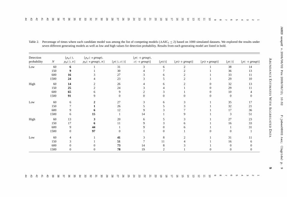
AB
UN
DA
NC
EE
ST
IMA
TE
SW
ITH
AG
GR
EG
AT
ED
DA
TA
9
11
22
33
44
55
66
77
88
99
1010
1111
1212
1313
1414
1515
1616
1717
1818
1919
2020
2121
2222
2323
2424
2525
2626
2727
2828
2929
3030
3131
3232
3333
3434
3535
3636
3737
3838
3939
4040
4141
4242
4343
4444
Table 2. Percentage of times where each candidate model was among the list of competing models (�AICc ≤ 2) based on 1000 simulated datasets. We explored the results underseven different generating models as well as low and high values for detection probability. Results from each generating model are listed in bold.
Detection {pa(·), {pa(· ∗ group), {p(· + group),
probability N pb(·),π} pb(· ∗ group),π} {p(·), c(·)} c(· + group)} {p(t)} {p(t + group)} {p(t ∗ group)} {p(·)} {p(· + group)}Low 60 6 1 31 3 6 2 1 38 14
150 9 1 30 4 7 2 1 36 13600 16 3 27 3 6 2 1 33 11
1500 24 4 23 3 5 2 1 29 10
High 60 14 2 26 4 6 2 0 32 13150 25 2 24 3 4 1 0 29 11600 65 6 9 2 3 1 0 10 4
1500 91 9 0 0 0 0 0 0 0
Low 60 6 2 27 3 6 3 1 35 17150 7 1 26 5 5 3 1 32 21600 9 6 12 9 3 7 1 17 36
1500 6 15 1 14 1 9 1 3 51
High 60 13 3 20 6 5 3 1 27 23150 17 6 11 9 3 6 1 16 33600 9 44 1 9 0 6 1 1 31
1500 0 97 0 1 0 1 0 0 1
Low 60 4 1 41 3 8 2 1 31 11150 3 1 51 7 11 4 1 16 6600 0 0 73 14 8 3 1 0 0
1500 0 0 78 19 2 1 0 0 0
JABES
asapdf
v.2009/06/02
Prn:2009/06/12;
10:52
F:jabes08002.tex;
(Ingrida)
p.
9
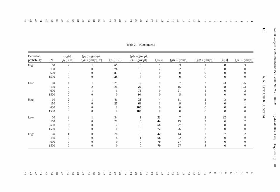
10A
.R.L
ITT
AN
DR
.J.ST
EID
L
11
22
33
44
55
66
77
88
99
1010
1111
1212
1313
1414
1515
1616
1717
1818
1919
2020
2121
2222
2323
2424
2525
2626
2727
2828
2929
3030
3131
3232
3333
3434
3535
3636
3737
3838
3939
4040
4141
4242
4343
4444
Table 2. (Continued.)
Detection {pa(·), {pa(· ∗ group), {p(· + group),
probability N pb(·),π} pb(· ∗ group),π} {p(·), c(·)} c(· + group)} {p(t)} {p(t + group)} {p(t ∗ group)} {p(·)} {p(· + group)}High 60 2 1 65 9 9 3 1 8 3
150 0 0 76 15 7 2 0 0 0600 0 0 83 17 0 0 0 0 0
1500 0 0 38 17 0 0 0 0 0
Low 60 4 1 29 5 5 7 2 23 25150 2 2 26 20 4 15 1 8 23600 0 1 1 75 0 21 1 0 2
1500 0 0 0 94 0 5 1 0 0
High 60 2 1 41 28 4 11 2 3 9150 0 0 25 64 1 9 1 0 1600 0 0 0 100 0 0 0 0 0
1500 0 0 0 100 0 0 0 0 0
Low 60 2 1 34 1 23 7 2 22 8150 0 0 29 3 44 15 2 6 2600 0 0 2 0 68 27 2 0 0
1500 0 0 0 0 72 26 2 0 0
High 60 1 0 28 3 42 14 2 7 2150 0 0 8 1 66 22 3 0 0600 0 0 0 0 70 27 3 0 0
1500 0 0 0 0 70 27 3 0 0
JABES
asapdf
v.2009/06/02
Prn:2009/06/12;
10:52
F:jabes08002.tex;
(Ingrida)
p.
10
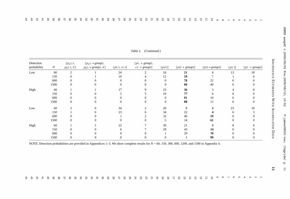
AB
UN
DA
NC
EE
ST
IMA
TE
SW
ITH
AG
GR
EG
AT
ED
DA
TA
11
11
22
33
44
55
66
77
88
99
1010
1111
1212
1313
1414
1515
1616
1717
1818
1919
2020
2121
2222
2323
2424
2525
2626
2727
2828
2929
3030
3131
3232
3333
3434
3535
3636
3737
3838
3939
4040
4141
4242
4343
4444
Table 2. (Continued.)
Detection {pa(·), {pa(· ∗ group), {p(· + group),
probability N pb(·),π} pb(· ∗ group),π} {p(·), c(·)} c(· + group)} {p(t)} {p(t + group)} {p(t ∗ group)} {p(·)} {p(· + group)}Low 60 2 1 24 2 16 21 4 13 18
150 0 1 10 4 12 59 7 1 6600 0 0 0 0 0 78 22 0 0
1500 0 0 0 0 0 60 40 0 0
High 60 1 1 17 9 23 36 3 4 8150 0 0 2 5 10 77 6 0 0600 0 0 0 0 0 91 10 0 0
1500 0 0 0 0 0 88 12 0 0
Low 60 2 0 34 2 20 8 2 23 10150 1 0 23 6 34 22 4 6 3600 0 0 1 2 32 46 19 0 0
1500 0 0 0 0 5 34 61 0 0
High 60 1 1 22 7 30 21 5 8 6150 0 0 6 7 29 43 14 0 0600 0 0 0 0 1 29 70 0 0
1500 0 0 0 0 0 1 99 0 0
NOTE: Detection probabilities are provided in Appendices 1–3. We show complete results for N = 60, 150, 300, 600, 1200, and 1500 in Appendix 4.
JABES
asapdf
v.2009/06/02
Prn:2009/06/12;
10:52
F:jabes08002.tex;
(Ingrida)
p.
11
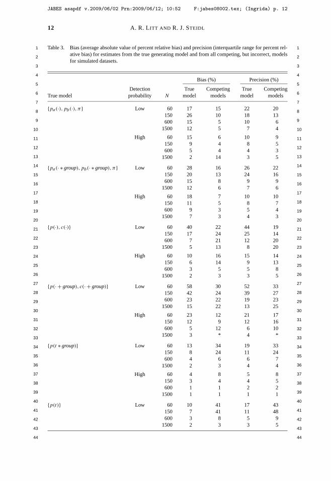
12 A. R. LITT AND R. J. STEIDL
1 1
2 2
3 3
4 4
5 5
6 6
7 7
8 8
9 9
10 10
11 11
12 12
13 13
14 14
15 15
16 16
17 17
18 18
19 19
20 20
21 21
22 22
23 23
24 24
25 25
26 26
27 27
28 28
29 29
30 30
31 31
32 32
33 33
34 34
35 35
36 36
37 37
38 38
39 39
40 40
41 41
42 42
43 43
44 44
Table 3. Bias (average absolute value of percent relative bias) and precision (interquartile range for percent rel-ative bias) for estimates from the true generating model and from all competing, but incorrect, modelsfor simulated datasets.
Bias (%) Precision (%)
Detection True Competing True CompetingTrue model probability N model models model models
{pa(·),pb(·),π} Low 60 17 15 22 20150 26 10 18 13600 15 5 10 6
1500 12 5 7 4
High 60 15 6 10 9150 9 4 8 5600 5 4 4 3
1500 2 14 3 5
{pa(· ∗ group),pb(· ∗ group),π} Low 60 28 16 26 22150 20 13 24 16600 15 8 9 9
1500 12 6 7 6
High 60 18 7 10 10150 11 5 8 7600 9 3 5 4
1500 7 3 4 3
{p(·), c(·)} Low 60 40 22 44 19150 17 24 25 14600 7 21 12 20
1500 5 13 8 20
High 60 10 16 15 14150 6 14 9 13600 3 5 5 8
1500 2 3 3 5
{p(· + group), c(· + group)} Low 60 58 30 52 33150 42 24 39 27600 23 22 19 23
1500 15 22 13 25
High 60 23 12 21 17150 12 9 12 16600 5 12 6 10
1500 3 * 4 *
{p(t ∗ group)} Low 60 13 34 19 33150 8 24 11 24600 4 6 6 7
1500 2 3 4 4
High 60 4 8 5 8150 3 4 4 5600 1 1 2 2
1500 1 1 1 1
{p(t)} Low 60 10 41 17 43150 7 41 11 48600 3 8 5 9
1500 2 3 3 5
JABES asapdf v.2009/06/02 Prn:2009/06/12; 10:52 F:jabes08002.tex; (Ingrida) p. 12
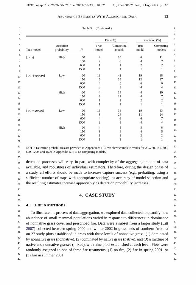
ABUNDANCE ESTIMATES WITH AGGREGATED DATA 13
1 1
2 2
3 3
4 4
5 5
6 6
7 7
8 8
9 9
10 10
11 11
12 12
13 13
14 14
15 15
16 16
17 17
18 18
19 19
20 20
21 21
22 22
23 23
24 24
25 25
26 26
27 27
28 28
29 29
30 30
31 31
32 32
33 33
34 34
35 35
36 36
37 37
38 38
39 39
40 40
41 41
42 42
43 43
44 44
Table 3. (Continued.)
Bias (%) Precision (%)
Detection True Competing True CompetingTrue model probability N model models model models
{p(t)} High 60 4 10 6 11150 2 6 4 7600 1 1 2 2
1500 1 1 1 1
{p(t + group)} Low 60 18 42 19 38150 9 39 12 37600 4 5 6 6
1500 3 3 4 4
High 60 4 14 4 10150 3 11 4 7600 1 1 2 2
1500 1 1 1 1
{p(t ∗ group)} Low 60 13 34 19 33150 8 24 11 24600 4 6 6 7
1500 2 3 4 4
High 60 4 8 5 8150 3 4 4 5600 1 1 2 2
1500 1 1 1 1
NOTE: Detection probabilities are provided in Appendices 1–3. We show complete results for N = 60, 150, 300,600, 1200, and 1500 in Appendix 5. ∗ = no competing models.
detection processes will vary, in part, with complexity of the aggregate, amount of dataavailable, and robustness of individual estimators. Therefore, during the design phase ofa study, all efforts should be made to increase capture success (e.g., prebaiting, using asufficient number of traps with appropriate spacing), as accuracy of model selection andthe resulting estimates increase appreciably as detection probability increases.
4. CASE STUDY
4.1 FIELD METHODS
To illustrate the process of data aggregation, we explored data collected to quantify howabundance of small mammal populations varied in response to differences in dominanceof nonnative grass cover and prescribed fire. Data were a subset from a larger study (Litt2007) collected between spring 2000 and winter 2002 in grasslands of southern Arizonaon 27 study plots established in areas with three levels of nonnative grass: (1) dominatedby nonnative grass (nonnative), (2) dominated by native grass (native), and (3) a mixture ofnative and nonnative grasses (mixed), with nine plots established at each level. Plots wererandomly assigned to one of three fire treatments: (1) no fire, (2) fire in spring 2001, or(3) fire in summer 2001.
JABES asapdf v.2009/06/02 Prn:2009/06/12; 10:52 F:jabes08002.tex; (Ingrida) p. 13
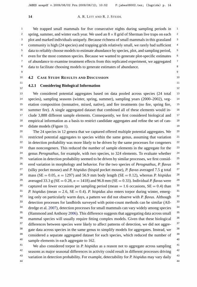
14 A. R. LITT AND R. J. STEIDL
1 1
2 2
3 3
4 4
5 5
6 6
7 7
8 8
9 9
10 10
11 11
12 12
13 13
14 14
15 15
16 16
17 17
18 18
19 19
20 20
21 21
22 22
23 23
24 24
25 25
26 26
27 27
28 28
29 29
30 30
31 31
32 32
33 33
34 34
35 35
36 36
37 37
38 38
39 39
40 40
41 41
42 42
43 43
44 44
We trapped small mammals for five consecutive nights during sampling periods inspring, summer, and winter each year. We used an 8× 8 grid of Sherman live traps on eachplot and marked individuals uniquely. Because richness of small mammals in this grasslandcommunity is high (24 species) and trapping grids relatively small, we rarely had sufficientdata to reliably choose models to estimate abundance by species, plot, and sampling period,even for the most common species. Because we wanted to generate plot-specific estimatesof abundance to examine treatment effects from this replicated experiment, we aggregateddata to facilitate choosing models to generate estimates of abundance.
4.2 CASE STUDY RESULTS AND DISCUSSION
4.2.1 Considering Biological Information
We considered potential aggregates based on data pooled across species (24 totalspecies), sampling seasons (winter, spring, summer), sampling years (2000–2002), veg-etation composition (nonnative, mixed, native), and fire treatments (no fire, spring fire,summer fire). A single aggregated dataset that combined all of these elements would in-clude 3,888 different sample elements. Consequently, we first considered biological andempirical information as a basis to restrict candidate aggregates and refine the set of can-didate models (Figure 1).
The 24 species in 12 genera that we captured offered multiple potential aggregates. Werestricted potential aggregates to species within the same genus, assuming that variationin detection probability was more likely to be driven by the same processes for congenersthan noncongeners. This reduced the number of sample elements in the aggregate for thegenus Perognathus, for example, with two species, to 324 elements. To evaluate whethervariation in detection probability seemed to be driven by similar processes, we first consid-ered variation in morphology and behavior. For the two species of Perognathus, P. flavus(silky pocket mouse) and P. hispidus (hispid pocket mouse), P. flavus averaged 7.5 g totalmass (SE = 0.05, n = 1297) and 56.9 mm body length (SE = 0.12), whereas P. hispidusaveraged 33.3 g (SE = 0.28, n = 1418) and 96.8 mm (SE = 0.33). Individual P. flavus werecaptured on fewer occasions per sampling period (mean = 1.6 occasions, SE = 0.4) thanP. hispidus (mean = 2.6, SE = 0.4). P. hispidus also enters torpor during winter, emerg-ing only on particularly warm days, a pattern we did not observe with P. flavus. Althoughdetection processes for landbirds surveyed with point-count methods can be similar (All-dredge et al. 2007), detection processes for small mammals can vary widely among species(Hammond and Anthony 2006). This difference suggests that aggregating data across smallmammal species will usually require fitting complex models. Given that these biologicaldifferences between species were likely to affect patterns of detection, we did not aggre-gate data across species in the same genus to simplify models for aggregates. Instead, weconsidered a separate aggregated dataset for each species, which reduced the number ofsample elements in each aggregate to 162.
We also considered torpor in P. hispidus as a reason not to aggregate across samplingseasons as major seasonal differences in activity could result in different processes drivingvariation in detection probability. For example, detectability for P. hispidus may vary daily
JABES asapdf v.2009/06/02 Prn:2009/06/12; 10:52 F:jabes08002.tex; (Ingrida) p. 14

ABUNDANCE ESTIMATES WITH AGGREGATED DATA 15
1 1
2 2
3 3
4 4
5 5
6 6
7 7
8 8
9 9
10 10
11 11
12 12
13 13
14 14
15 15
16 16
17 17
18 18
19 19
20 20
21 21
22 22
23 23
24 24
25 25
26 26
27 27
28 28
29 29
30 30
31 31
32 32
33 33
34 34
35 35
36 36
37 37
38 38
39 39
40 40
41 41
42 42
43 43
44 44
with variation in temperature during winter, where a temporal model of detection probabil-ity might be most appropriate. This model might be less appropriate in other seasons whenthese animals are consistently active, more detectable, and somewhat trap-happy. We choseto apply the same aggregation strategy for all species; therefore, if a level of aggregationwas not supported for some species or circumstances, we rejected that level for all species.As such, we considered a separate aggregated dataset for each species and each season,reducing the number of elements in each aggregate to 54.
We could not envision a biological reason why the process driving variation in detectionprobability would differ among years for a given season or vary with the amount of non-native grass, therefore, for each species we aggregated data over years and over levels ofvegetation composition. Because we were interested in comparing changes in abundancein response to prescribed fire treatments, we also considered aggregating over fire season.By including plots that received different fire treatments in the same aggregate, we avoidedconfounding potential biases due to model choice with any treatment effects. Therefore,we created aggregated datasets for each species and season that included multiple sam-pling years, all levels of vegetation composition, and all fire treatments.
4.2.2 Modeling Detection Probability
Although 54 aggregated elements and the resulting candidate models seemed relativelyreasonable, we explored support for this candidate aggregate empirically, using the rich-est datasets from potential elements—plots or sets of plots that received the same treat-ment and were sampled at the same time. For P. flavus, we considered eight datasets, eachwith 45–101 captured individuals (Table 4). These datasets represented all sampling years(5 datasets for 2000, 2 for 2001, and 2 for 2002), all categories of vegetation composition(5 datasets for native, 2 for mixed, and 1 for nonnative), but only unburned areas. We usedthese data to explore eight general models for detection probability (Table 1) and gaugedconsistency in the set of competing models (�AICc ≤ 2) for datasets from different years,vegetation composition categories, or fire treatments (Table 4). A general model with tem-poral variation was among competing models for 7 of 8 datasets and was the model with
Table 4. Competing general models (�AICc ≤ 2) and number of individuals captured (Mt+1) for individualdatasets for Perognathus flavus.
Data set Season Year Vegetation Mt+1 Competing models
1 Spring 2000 Mixed 45 {p(·), c(·)}, {p(·)}, {p(t)}2 Winter 2002 Native 45 {p(t)}3 Summer 2000 Nonnative 46 {p(·)}, {pa(·),pb(·),π}, {p(·), c(·)}4 Spring 2001 Native 48 {p(·)}, {p(t)}5 Summer 2001 Native 61 {p(t)}6 Summer 2000 Native 87 {pa(·),pb(·),π}, {p(t)}7 Spring 2000 Native 97 {p(t)}8 Summer 2000 Mixed 101 {p(t)}, {pa(t),pb(t),π}
NOTE: Datasets included sets of plots sampled at the same time and that received the same treatment. Competinggeneral models are listed in order of increasing AICc value.
JABES asapdf v.2009/06/02 Prn:2009/06/12; 10:52 F:jabes08002.tex; (Ingrida) p. 15
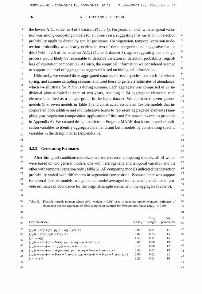
16 A. R. LITT AND R. J. STEIDL
1 1
2 2
3 3
4 4
5 5
6 6
7 7
8 8
9 9
10 10
11 11
12 12
13 13
14 14
15 15
16 16
17 17
18 18
19 19
20 20
21 21
22 22
23 23
24 24
25 25
26 26
27 27
28 28
29 29
30 30
31 31
32 32
33 33
34 34
35 35
36 36
37 37
38 38
39 39
40 40
41 41
42 42
43 43
44 44
the lowest AICc value for 4 of 8 datasets (Table 4). For years, a model with temporal varia-
tion was among competing models for all three years, suggesting that variation in detection
probability might be driven by similar processes. For vegetation, temporal variation in de-
tection probability was clearly evident in two of three categories and suggestive for the
third (within 2.5 of the smallest AICc) (Table 4, dataset 3), again suggesting that a single
process would likely be reasonable to describe variation in detection probability, regard-
less of vegetation composition. As such, the empirical information we considered seemed
to support the level of aggregation suggested based on biological information.
Ultimately, we created three aggregated datasets for each species, one each for winter,
spring, and summer sampling seasons, and used these to generate estimates of abundance,
which we illustrate for P. flavus during summer. Each aggregate was comprised of 27 in-
dividual plots sampled in each of two years, resulting in 54 aggregated elements, each
element identified as a unique group in the input dataset. We considered seven general
models (first seven models in Table 1) and constructed associated flexible models that in-
corporated both additive and multiplicative terms to represent aggregated elements (sam-
pling year, vegetation composition, application of fire, and fire season; examples provided
in Appendix 6). We created design matrices in Program MARK that incorporated classifi-
cation variables to identify aggregated elements and built models by constraining specific
variables in the design matrix (Appendix 6).
4.2.3 Generating Estimates
After fitting all candidate models, there were several competing models, all of which
were based on two general models, one with heterogeneity and temporal variation and the
other with temporal variation only (Table 5). All competing models indicated that detection
probability varied with differences in vegetation composition. Because there was support
for several flexible models, we generated model-averaged estimates of abundance to pro-
vide estimates of abundance for the original sample elements in the aggregate (Table 6).
Table 5. Flexible models (shown where AICc weight ≥ 0.01) used to generate model-averaged estimates ofabundance for the aggregate of plots sampled in summer for Perognathus flavus (Mt+1 = 319).
AICc No.Flexible model �AICc weight parameters
{pa(t + veg + yr),pb(t + veg + yr),π} 0.00 0.37 17{pa(t + veg),pb(t + veg),π} 0.82 0.25 15{p(t ∗ veg)} 1.58 0.17 15{pa(t + veg + yr + burn),pb(t + veg + yr + burn),π} 3.07 0.08 19{pa(t + veg + burn),pb(t + veg + burn),π} 3.19 0.08 17{pa(t + veg + burn + fireseas),pb(t + veg + burn + fireseas),π} 5.45 0.02 19{pa(t + veg + yr + burn + fireseas),pb(t + veg + yr + burn + fireseas),π} 5.80 0.02 21{p(t ∗ yr)} 8.28 0.01 10
JABES asapdf v.2009/06/02 Prn:2009/06/12; 10:52 F:jabes08002.tex; (Ingrida) p. 16
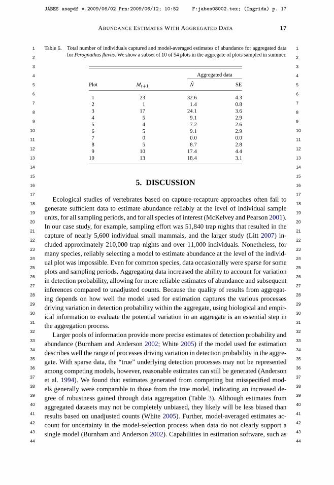
ABUNDANCE ESTIMATES WITH AGGREGATED DATA 17
1 1
2 2
3 3
4 4
5 5
6 6
7 7
8 8
9 9
10 10
11 11
12 12
13 13
14 14
15 15
16 16
17 17
18 18
19 19
20 20
21 21
22 22
23 23
24 24
25 25
26 26
27 27
28 28
29 29
30 30
31 31
32 32
33 33
34 34
35 35
36 36
37 37
38 38
39 39
40 40
41 41
42 42
43 43
44 44
Table 6. Total number of individuals captured and model-averaged estimates of abundance for aggregated datafor Perognathus flavus. We show a subset of 10 of 54 plots in the aggregate of plots sampled in summer.
Aggregated data
Plot Mt+1 N̂ SE
1 23 32.6 4.32 1 1.4 0.83 17 24.1 3.64 5 9.1 2.95 4 7.2 2.66 5 9.1 2.97 0 0.0 0.08 5 8.7 2.89 10 17.4 4.4
10 13 18.4 3.1
5. DISCUSSION
Ecological studies of vertebrates based on capture-recapture approaches often fail togenerate sufficient data to estimate abundance reliably at the level of individual sampleunits, for all sampling periods, and for all species of interest (McKelvey and Pearson 2001).In our case study, for example, sampling effort was 51,840 trap nights that resulted in thecapture of nearly 5,600 individual small mammals, and the larger study (Litt 2007) in-cluded approximately 210,000 trap nights and over 11,000 individuals. Nonetheless, formany species, reliably selecting a model to estimate abundance at the level of the individ-ual plot was impossible. Even for common species, data occasionally were sparse for someplots and sampling periods. Aggregating data increased the ability to account for variationin detection probability, allowing for more reliable estimates of abundance and subsequentinferences compared to unadjusted counts. Because the quality of results from aggregat-ing depends on how well the model used for estimation captures the various processesdriving variation in detection probability within the aggregate, using biological and empir-ical information to evaluate the potential variation in an aggregate is an essential step inthe aggregation process.
Larger pools of information provide more precise estimates of detection probability andabundance (Burnham and Anderson 2002; White 2005) if the model used for estimationdescribes well the range of processes driving variation in detection probability in the aggre-gate. With sparse data, the “true” underlying detection processes may not be representedamong competing models, however, reasonable estimates can still be generated (Andersonet al. 1994). We found that estimates generated from competing but misspecified mod-els generally were comparable to those from the true model, indicating an increased de-gree of robustness gained through data aggregation (Table 3). Although estimates fromaggregated datasets may not be completely unbiased, they likely will be less biased thanresults based on unadjusted counts (White 2005). Further, model-averaged estimates ac-count for uncertainty in the model-selection process when data do not clearly support asingle model (Burnham and Anderson 2002). Capabilities in estimation software, such as
JABES asapdf v.2009/06/02 Prn:2009/06/12; 10:52 F:jabes08002.tex; (Ingrida) p. 17
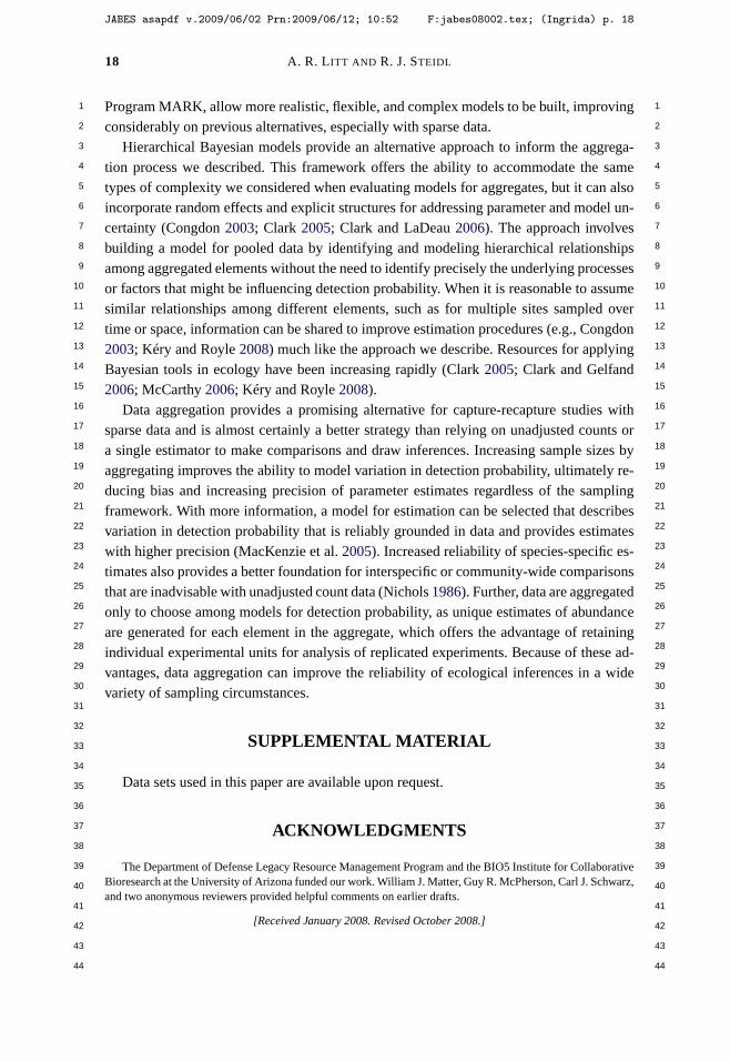
18 A. R. LITT AND R. J. STEIDL
1 1
2 2
3 3
4 4
5 5
6 6
7 7
8 8
9 9
10 10
11 11
12 12
13 13
14 14
15 15
16 16
17 17
18 18
19 19
20 20
21 21
22 22
23 23
24 24
25 25
26 26
27 27
28 28
29 29
30 30
31 31
32 32
33 33
34 34
35 35
36 36
37 37
38 38
39 39
40 40
41 41
42 42
43 43
44 44
Program MARK, allow more realistic, flexible, and complex models to be built, improvingconsiderably on previous alternatives, especially with sparse data.
Hierarchical Bayesian models provide an alternative approach to inform the aggrega-tion process we described. This framework offers the ability to accommodate the sametypes of complexity we considered when evaluating models for aggregates, but it can alsoincorporate random effects and explicit structures for addressing parameter and model un-certainty (Congdon 2003; Clark 2005; Clark and LaDeau 2006). The approach involvesbuilding a model for pooled data by identifying and modeling hierarchical relationshipsamong aggregated elements without the need to identify precisely the underlying processesor factors that might be influencing detection probability. When it is reasonable to assumesimilar relationships among different elements, such as for multiple sites sampled overtime or space, information can be shared to improve estimation procedures (e.g., Congdon2003; Kéry and Royle 2008) much like the approach we describe. Resources for applyingBayesian tools in ecology have been increasing rapidly (Clark 2005; Clark and Gelfand2006; McCarthy 2006; Kéry and Royle 2008).
Data aggregation provides a promising alternative for capture-recapture studies withsparse data and is almost certainly a better strategy than relying on unadjusted counts ora single estimator to make comparisons and draw inferences. Increasing sample sizes byaggregating improves the ability to model variation in detection probability, ultimately re-ducing bias and increasing precision of parameter estimates regardless of the samplingframework. With more information, a model for estimation can be selected that describesvariation in detection probability that is reliably grounded in data and provides estimateswith higher precision (MacKenzie et al. 2005). Increased reliability of species-specific es-timates also provides a better foundation for interspecific or community-wide comparisonsthat are inadvisable with unadjusted count data (Nichols 1986). Further, data are aggregatedonly to choose among models for detection probability, as unique estimates of abundanceare generated for each element in the aggregate, which offers the advantage of retainingindividual experimental units for analysis of replicated experiments. Because of these ad-vantages, data aggregation can improve the reliability of ecological inferences in a widevariety of sampling circumstances.
SUPPLEMENTAL MATERIAL
Data sets used in this paper are available upon request.
ACKNOWLEDGMENTS
The Department of Defense Legacy Resource Management Program and the BIO5 Institute for CollaborativeBioresearch at the University of Arizona funded our work. William J. Matter, Guy R. McPherson, Carl J. Schwarz,and two anonymous reviewers provided helpful comments on earlier drafts.
[Received January 2008. Revised October 2008.]
JABES asapdf v.2009/06/02 Prn:2009/06/12; 10:52 F:jabes08002.tex; (Ingrida) p. 18
ABUNDANCE ESTIMATES WITH AGGREGATED DATA 19
1 1
2 2
3 3
4 4
5 5
6 6
7 7
8 8
9 9
10 10
11 11
12 12
13 13
14 14
15 15
16 16
17 17
18 18
19 19
20 20
21 21
22 22
23 23
24 24
25 25
26 26
27 27
28 28
29 29
30 30
31 31
32 32
33 33
34 34
35 35
36 36
37 37
38 38
39 39
40 40
41 41
42 42
43 43
44 44
REFERENCES
Alldredge, M. W., Pollock, K. H., Simons, T. R., and Shriner, S. A. (2007), “Multiple-Species Analysis of PointCount Data: A More Parsimonious Modelling Framework,” Journal of Applied Ecology, 44, 281–290.
Anderson, D. R., Burnham, K. P., and White, G. C. (1994), “AIC Model Selection in Overdispersed Capture-Recapture Data,” Ecology, 75, 1780–1793.
Bowden, D. C., White, G. C., Franklin, A. B., and Ganey, J. L. (2003), “Estimating Population Size With Corre-lated Sampling Unit Estimates,” Journal of Wildlife Management, 67, 1–10.
Boyce, M. S., MacKenzie, D. I., Manly, B. F. J., Haroldson, M. A., and Moody, D. (2001), “Negative BinomialModels for Abundance Estimation of Multiple Closed Populations,” Journal of Wildlife Management, 65,498–509.
Buckland, S. T., Anderson, D. R., Burnham, K. P., and Laake, J. L. (1993), Distance Sampling: EstimatingAbundance of Biological Populations, New York: Chapman & Hall.
Burnham, K. P., and Anderson, D. R. (2002), Model Selection and Multimodel Inference: A Practical Information-Theoretic Approach (2nd ed.), New York: Springer.
Clark, J. S. (2005), “Why Environmental Scientists Are Becoming Bayesians,” Ecology Letters, 8, 2–14.
Clark, J. S., and Gelfand, A. E. (eds.) (2006), Hierarchical Modeling for the Environmental Sciences, Oxford:Oxford University Press.
Clark, J. S., and LaDeau, S. (2006), “Synthesizing Ecological Experiments and Observational Data With Hierar-chical Bayes,” in Hierarchical Modeling for the Environmental Sciences, eds. J. S. Clark and A. E. Gelfand,Oxford: Oxford University Press, pp. 41–58.
Congdon, P. (2003), Applied Bayesian Modelling, West Sussex: Wiley.
Conn, P. B., Arthur, A. D., Bailey, L. L., and Singleton, G. R. (2006), “Estimating the Abundance of MousePopulations of Known Size: Promises and Pitfalls of New Methods,” Ecological Applications, 16, 829–837.
Hammond, E. L., and Anthony, R. G. (2006), “Mark-Recapture Estimates of Population Parameters for SelectedSpecies of Small Mammals,” Journal of Mammalogy, 87, 618–627.
Hargrove, J. W., and Borland, C. H. (1994), “Pooled Population Parameter Estimates From Mark-RecaptureData,” Biometrics, 50, 1129–1141.
Kéry, M., and Royle, J. A. (2008), “Hierarchical Bayes Estimation of Species Richness and Occupancy in Spa-tially Replicated Surveys,” Journal of Applied Ecology, 45, 589–598.
Litt, A. R. (2007), “Effects of Experimental Fire and Nonnative Grass Invasion on Small Mammals and Insects,”unpublished Ph.D. dissertation, University of Arizona, School of Natural Resources.
Lynam, A. J., Rabinowitz, A., Myint, T., Maung, M., Latt, K. T., and Po, A. H. T. (2008), “Estimating AbundanceWith Sparse Data: Tigers in Northern Myanmar,” Population Ecology, 50, DOI: 10.1007/s10144-008-0093-5.
MacKenzie, D. I., and Kendall, W. L. (2002), “How Should Detection Probability Be Incorporated Into Estimatesof Relative Abundance?” Ecology, 83, 2327–2393.
MacKenzie, D. I., Nichols, J. D., Sutton, N., Kawanishi, K., and Bailey, L. L. (2005), “Improving Inferences inPopulation Studies of Rare Species That Are Detected Imperfectly,” Ecology, 86, 1101–1113.
McCarthy, M. A. (2006), Bayesian Methods for Ecology, Cambridge: Cambridge University Press.
McKelvey, K. S., and Pearson, D. E. (2001), “Population Estimation With Sparse Data: The Role of Estimatorsversus Indices Revisited,” Canadian Journal of Zoology, 79, 1754–1765.
Nichols, J. D. (1986), “On the Use of Enumeration Estimators for Interspecific Comparisons, With Comments ona ‘Trappability’ Estimator,” Journal of Mammalogy, 67, 590–593.
(1992), “Capture-Recapture Models: Using Marked Animals to Study Population Dynamics,” Bio-Science, 42, 94–102.
Otis, D. L., Burnham, K. P., White, G. C., and Anderson, D. R. (1978), “Statistical Inference From Capture Dataon Closed Animal Populations,” Wildlife Monographs, 62, 1–135.
Rosenberg, D. K., Overton, W. S., and Anthony, R. G. (1995), “Estimation of Animal Abundance When CaptureProbabilities Are Low and Heterogeneous,” Journal of Wildlife Management, 59, 252–261.
JABES asapdf v.2009/06/02 Prn:2009/06/12; 10:52 F:jabes08002.tex; (Ingrida) p. 19

20 A. R. LITT AND R. J. STEIDL
1 1
2 2
3 3
4 4
5 5
6 6
7 7
8 8
9 9
10 10
11 11
12 12
13 13
14 14
15 15
16 16
17 17
18 18
19 19
20 20
21 21
22 22
23 23
24 24
25 25
26 26
27 27
28 28
29 29
30 30
31 31
32 32
33 33
34 34
35 35
36 36
37 37
38 38
39 39
40 40
41 41
42 42
43 43
44 44
Rosenberg, D. K., Swindle, K. A., and Anthony, R. G. (2003), “Influence of Prey Abundance on Northern SpottedOwl Reproductive Success in Western Oregon,” Canadian Journal of Zoology, 81, 1715–1725.
Schwarz, C. J., and Seber, G. A. F. (1999), “Estimating Animal Abundance: Review III,” Statistical Science, 14,427–456.
Seber, G. A. F. (1982), Estimation of Animal Abundance and Related Parameters, New York: Macmillan.
(1986), “A Review of Estimating Animal Abundance,” Biometrics, 42, 267–292.
(1992), “A Review of Estimating Animal Abundance II,” International Statistical Review, 60, 129–166.
Skalski, J. R., Robson, D. S., and Simmons, M. A. (1983), “Comparative Census Procedures Using Single Mark-Recapture Methods,” Ecology, 64, 752–760.
White, G. C. (2005), “Correcting Wildlife Counts Using Detection Probabilities,” Wildlife Research, 32, 211–216.
White, G. C., and Burnham, K. P. (1999), “Program MARK: Survival Estimation From Populations of MarkedAnimals,” Bird Study, 46 (Suppl.), 120–138.
JABES asapdf v.2009/06/02 Prn:2009/06/12; 10:52 F:jabes08002.tex; (Ingrida) p. 20
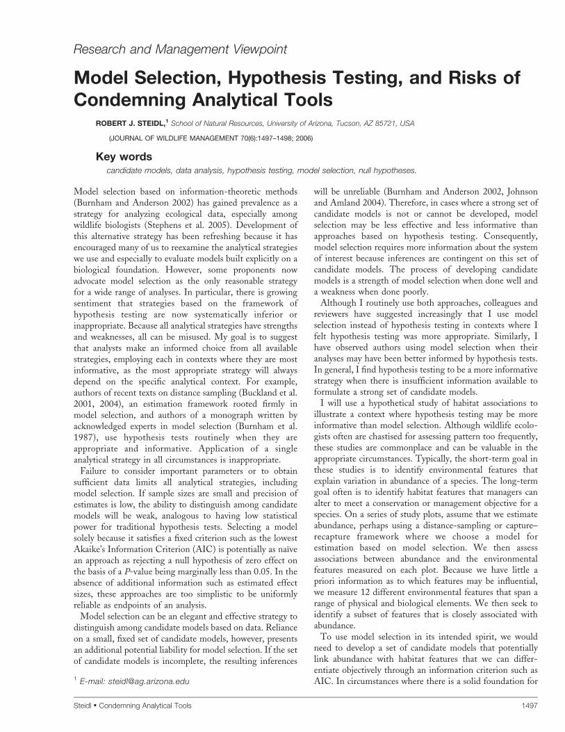
Research and Management Viewpoint
Model Selection, Hypothesis Testing, and Risks ofCondemning Analytical Tools
ROBERT J. STEIDL,1 School of Natural Resources, University of Arizona, Tucson, AZ 85721, USA
(JOURNAL OF WILDLIFE MANAGEMENT 70(6):1497–1498; 2006)
Key wordscandidate models, data analysis, hypothesis testing, model selection, null hypotheses.
Model selection based on information-theoretic methods(Burnham and Anderson 2002) has gained prevalence as astrategy for analyzing ecological data, especially amongwildlife biologists (Stephens et al. 2005). Development ofthis alternative strategy has been refreshing because it hasencouraged many of us to reexamine the analytical strategieswe use and especially to evaluate models built explicitly on abiological foundation. However, some proponents nowadvocate model selection as the only reasonable strategyfor a wide range of analyses. In particular, there is growingsentiment that strategies based on the framework ofhypothesis testing are now systematically inferior orinappropriate. Because all analytical strategies have strengthsand weaknesses, all can be misused. My goal is to suggestthat analysts make an informed choice from all availablestrategies, employing each in contexts where they are mostinformative, as the most appropriate strategy will alwaysdepend on the specific analytical context. For example,authors of recent texts on distance sampling (Buckland et al.2001, 2004), an estimation framework rooted firmly inmodel selection, and authors of a monograph written byacknowledged experts in model selection (Burnham et al.1987), use hypothesis tests routinely when they areappropriate and informative. Application of a singleanalytical strategy in all circumstances is inappropriate.
Failure to consider important parameters or to obtainsufficient data limits all analytical strategies, includingmodel selection. If sample sizes are small and precision ofestimates is low, the ability to distinguish among candidatemodels will be weak, analogous to having low statisticalpower for traditional hypothesis tests. Selecting a modelsolely because it satisfies a fixed criterion such as the lowestAkaike’s Information Criterion (AIC) is potentially as naı̈vean approach as rejecting a null hypothesis of zero effect onthe basis of a P-value being marginally less than 0.05. In theabsence of additional information such as estimated effectsizes, these approaches are too simplistic to be uniformlyreliable as endpoints of an analysis.
Model selection can be an elegant and effective strategy todistinguish among candidate models based on data. Relianceon a small, fixed set of candidate models, however, presentsan additional potential liability for model selection. If the setof candidate models is incomplete, the resulting inferences
will be unreliable (Burnham and Anderson 2002, Johnsonand Amland 2004). Therefore, in cases where a strong set ofcandidate models is not or cannot be developed, modelselection may be less effective and less informative thanapproaches based on hypothesis testing. Consequently,model selection requires more information about the systemof interest because inferences are contingent on this set ofcandidate models. The process of developing candidatemodels is a strength of model selection when done well anda weakness when done poorly.
Although I routinely use both approaches, colleagues andreviewers have suggested increasingly that I use modelselection instead of hypothesis testing in contexts where Ifelt hypothesis testing was more appropriate. Similarly, Ihave observed authors using model selection when theiranalyses may have been better informed by hypothesis tests.In general, I find hypothesis testing to be a more informativestrategy when there is insufficient information available toformulate a strong set of candidate models.
I will use a hypothetical study of habitat associations toillustrate a context where hypothesis testing may be moreinformative than model selection. Although wildlife ecolo-gists often are chastised for assessing pattern too frequently,these studies are commonplace and can be valuable in theappropriate circumstances. Typically, the short-term goal inthese studies is to identify environmental features thatexplain variation in abundance of a species. The long-termgoal often is to identify habitat features that managers canalter to meet a conservation or management objective for aspecies. On a series of study plots, assume that we estimateabundance, perhaps using a distance-sampling or capture–recapture framework where we choose a model forestimation based on model selection. We then assessassociations between abundance and the environmentalfeatures measured on each plot. Because we have little apriori information as to which features may be influential,we measure 12 different environmental features that span arange of physical and biological elements. We then seek toidentify a subset of features that is closely associated withabundance.
To use model selection in its intended spirit, we wouldneed to develop a set of candidate models that potentiallylink abundance with habitat features that we can differ-entiate objectively through an information criterion such asAIC. In circumstances where there is a solid foundation for1 E-mail: [email protected]
Steidl � Condemning Analytical Tools 1497
selecting candidate models, this is a powerful approach. Insituations such as this example, however, where there is littleinformation available and 4,095 potential models (manymore if we consider interactions), model selection is likely tobe less informative than alternative strategies simply becauseany small set of candidate models is likely to be inadequate.
I am not suggesting that these types of habitat-associationstudies are particularly efficient; rather I recognize only thatthey are common when there is little published informationavailable about a phenomenon. I also recognize that if thestudy design is sound and patterns in the data are robust,experienced analysts likely would find similar patternsregardless of their chosen strategy. My concerns are forinexperienced analysts.
I recently reviewed a paper that fits the above examplewell, a study where apparently little information wasavailable for developing meaningful candidate models. Thestudy design was straightforward, with abundance and alarge suite of habitat variables measured on scores of plots.The authors chose model selection for their analyses, buttheir candidate set consisted of only 4 models linkingabundance to habitat features, one of which they justified bysuggesting that they could think of no good reason not toconsider it. Although it might be easiest to attribute thissmall set of models to a lack of critical thinking, incircumstances such as this I argue that it can be challengingto think of a combination of variables that would not formthe basis for a tenable model. So despite a reasonable study,
the authors ultimately extracted only a minute amount of
the information that they had gathered on the question of
interest, in part, because they sought to keep the number ofcandidate models small. In cases where the process of
selecting a set of candidate models is more an exercise rather
than a strategy to distinguish among carefully derivedalternatives, model selection will not be an effective strategy
for analysis (Burnham and Anderson 2002).
For a circumstance such as this, I might have recom-mended stepwise variable-selection with limits for selection
set liberally (one of which could be AIC), with the caveat
that no set of explanatory variables be considered sacrosanct
without additional investigation. Although certainly not ascalpel, variable-selection strategies such as this remain a
reasonable approach for efficiently considering a large
number of unstructured models. A similar approach basedon model selection would involve fitting all possible models,
but that approach runs counter to the philosophy of model
selection. If the original objective of the study was morefocused, then a model-selection strategy based on a pithy set
of candidate models would be entirely appropriate.
Tools based on hypothesis testing will continue to beuseful in many circumstances, especially when used
thoughtfully. Abandonment of this strategy or wholesale
adoption of any other can only serve to limit the generationof new scientific knowledge in wildlife ecology and other
disciplines.
Literature Cited
Buckland, S. T., D. R. Anderson, K. P. Burnham, J. L. Laake, D. L.Borchers, and L. Thomas. 2001. An introduction to distancesampling: estimating abundance of biological populations. OxfordUniversity, United Kingdom.
Buckland, S. T., D. R. Anderson, K. P. Burnham, J. L. Laake, D. L.Borchers, and L. Thomas. 2004. Advanced distance sampling:estimating abundance of biological populations. Oxford University,United Kingdom.
Burnham, K. P., and D. R. Anderson. 2002. Model selection andinference: a practical information-theoretic approach. Second edition.Springer, New York, New York, USA.
Burnham, K. P., D. R. Anderson, G. C. White, C. Brownie, and K. H.Pollock. 1987. Design and analysis of fish survival experiments basedon release–recapture data. American Fisheries Society, Bethesda,Maryland, USA.
Johnson, J. B., and K. S. Omland. 2004. Model selection in ecologyand evolution. Trends in Ecology and Evolution 19:101–108.
Stephens, P. A., S. W. Buskirk, G. D. Hayward, and C. Martinez del Rio.2005. Information theory and hypothesis testing: a call for pluralism.Journal of Applied Ecology 42:4–12.
Associate Editor: Morrison.
1498 The Journal of Wildlife Management � 70(6)
Given the breadth of relevant humanactivities, the diversity of wildlife speciespotentially affected, and the multitude ofways they may be affected, scientists andresource managers planning to assess theeffects of human activities on wildlife mustbe careful to state their study objectivesexplicitly. In all cases, these objectivesshould specify the human activity of inter-est; the timing, intensity (frequency, dura-tion) and spatial extent of the activity; thefocal wildlife species of interest; and therange of ways that species might respond tothe activity—that is, the objectives shoulddefine the “disturbance context” in whichthe human–wildlife interaction occurs(Steidl and Anthony 2000). Given well-defined objectives and a clear disturbancecontext, a measure that gauges the responseof the wildlife species of interest to thehuman activity must be selected carefully.
In this paper, we provide a general clas-sification for the ways in which humanactivities can affect wildlife, distinguishamong general types of relevant studies
based on different objectives, and identifyappropriate measures for gauging wildliferesponse for different types of studies. Ourgoal is to provide a conceptual frameworkto guide studying and monitoring human–wildlife interactions, specifically thosederiving from non-consumptive recreation-al activities.
Classifying human activitiesVirtually all human activities can affect
wildlife populations either positively ornegatively. Those activities that are likely tohave adverse effects can be divided intothose that function primarily by altering thephysical environment in a relatively perma-nent way and those that cause changes to ananimal’s behavior. Activities that alter thephysical environment change the amount orthe suitability of habitat for a species.Widespread and large-scale examplesinclude activities that directly alter thestructure and composition of the landscape,such agriculture, forestry, livestock grazing,and unregulated off-road vehicle use. In
The George Wright Forum50
Assessing the Effects of Human Activities on Wildlife
Robert J. Steidl and Brian F. Powell
HUMAN ACTIVITIES THAT AFFECT WILDLIFE AND THEIR HABITATS are pervasive and increas-ing. Effects of these activities are manifested at all ecological scales, from short-term changesin the behavior of an individual animal through local extirpations and global extinctions(Pimm et al. 1995; Chapin et al. 2000). Consequently, understanding the effects of humanson wildlife and wildlife populations, as well as devising strategies to ameliorate these effects,is an increasing challenge for resource managers. Given the conflicting mandate to bothencourage human use and to protect sensitive natural resources in national parks, develop-ing reliable strategies for assessing and monitoring the effects of human activities on naturalresources is essential to ensuring appropriate stewardship of these resources.
general, these are land use or land manage-ment practices that change the trajectory ofecological succession, including altering thedominant plant communities and the abiot-ic features of a site. The ecological effects ofthese activities on vertebrates are readilyapparent and have been relatively well stud-ied (e.g., Blair 1996; Spies et al. 1996;Lichstein et al. 2002).
Perhaps less obvious in their ecologicalimpacts are those non-consumptive humanactivities that do not appreciably alter thephysical environment but nonetheless canaffect wildlife adversely. Examples includerecreational activities such as hiking,wildlife viewing, and boating—all commonactivities for visitors in parks. As recreation-al use increases in wilderness and otherprotected areas, sensitive wildlife speciesmay be increasingly affected by these activi-ties (Steidl and Anthony 2000). The magni-tude of effects of recreational activities onwildlife is influenced by many factors,including the type, duration, frequency,magnitude, location, and timing of the dis-turbance, as well as the particular species ofinterest. Although effects of these activitiesare typically of short duration, cumulativelythey can effect wildlife populations adverse-ly in both the short- and long-term (Burger1981; Henson and Grant 1991; Fernandezand Azkona 1993; Holmes et al. 1994;Steidl and Anthony 1996, 2000; Swarthoutand Steidl 2001, 2003; Mann et al. 2002;Johnson et al. 2005). Observed effects in-clude increased energetic stresses (Bélangerand Bédard 1990), changes in activitybudgets (Steidl and Anthony 2000; Mannet al. 2002; Swarthout and Steidl 2001,2003), displacement from preferred envi-ronments (McGarigal et al. 1991), andreduced productivity through abandon-ment and decreased survival of young
(Tremblay and Ellison 1979; White andThurow 1985).
Although there are human activitiesthat cause physical changes to park environ-ments, such as construction of building androads, or vegetation destruction resultingfrom overuse of particular areas, mostwildlife-related impacts away from theseareas likely result from short-term recre-ational pursuits of visitors. We focus theremainder of our discussion on these typesof activities.
Types of studiesGiven the wide range of potential infor-
mation needs and study objectives, we dis-tinguish between two fundamentally differ-ent kinds of studies: research and monitor-ing. These can be classified primarily basedon their different objectives and secondarilybased on different durations. Research stud-ies include an objective related to answeringspecific questions and are usually of rela-tively short duration (1–3 years). An exam-ple would be a study conceived to assess thedistance at which a population of birdsflushes in response to a particular visitoractivity, such as hiking or mountain biking(e.g., Swarthout and Steidl 2001). The goalfor this type of study might be to reliablyestablish the distance at which birds flush inresponse to the activity so that the activitycan be restricted in particular areas toreduce disturbance frequency and mini-mize adverse effects. In contrast, monitor-ing studies involve quantifying changes incharacteristics of resources over time, areusually not driven by particular questions,and are always intended to be undertakenover long-time periods (Steidl 2001). Thegoal for monitoring studies is almost alwaysrelated to quantifying changes in character-istics of resources over time. A third kind of
Visitor Impact Monitoring
Volume 23 • Number 2 (2006) 51
study, which we only mention here, is ahybrid between research and monitoringstudies. Impact assessment studies are de-signed to measure the effects of a plannedactivity or action within the context of a pre-viously established monitoring program.These are often large-scale studies wherethe fundamental approach is to establish amonitoring program based on a series ofsampling sites, a subset of which is eventu-ally subject to being affected by the impact.The effect of the impact is estimated bycomparing how sites subject to the impactchange relative to control or reference sitesover time (Green 1979). The application ofthese studies is useful to natural resourcemanagers interested in assessing the effectsof management actions, such as opening orclosing particular trails or other facilities,especially when replication of the impact isimpossible.
All types of studies benefit from carefulapplication of the basic tools of researchdesign, which include randomization, repli-cation, reduction of error, incorporation ofadequate controls, and understanding howthe scope of inference for any study is dic-tated in part by the way study units areselected (Ramsey and Shafer 2001).
Research studies. Specific resourcemanagement questions about human–wildlife interactions are best answeredthrough well-designed research studies,either experimental or observational. Ques-tions that can be answered experimentally,which always involves some type of manip-ulation by the investigators, are more pow-erful than observational studies becausethey provide strong evidence of a causallink between the activity and the responsemeasure. Observational studies cannotestablish cause-and-effect inferences be-cause of the potential for confounding by
additional factors that may have influencedthe response measure. Observational stud-ies, therefore, provide only correlative infer-ences, yet can offer strong evidence whendesigned carefully. There is a vast literatureon conceiving and designing effectiveresearch studies on wildlife populations(e.g., Morrison et al. 2001).
Monitoring. Ecological monitoringstudies almost always focus on quantifyingchanges in characteristics of resources overtime. Consequently, monitoring studies arecorrelative and can therefore quantify pat-terns and associations but cannot establishcausal links between changes in theresource of interest and changes in levels ofhuman activity or other environmentalcharacteristics. For example, if we observe adecline in abundance of a species in an areaover time concurrent with an increase in aparticular type of human activity, we cannotclaim that the increase in human activitycaused the decrease in abundance. Despitetheir limited inference relative to random-ized experiments, monitoring studies canstill provide information that is valuable forunderstanding and reducing human–wildlife conflicts (Burger et al. 2004) espe-cially when designed as part of an integrat-ed monitoring program that encompasses arange of biotic and abiotic resources.Specifically, by measuring other environ-mental characteristics that are thought toaffect changes in the wildlife response meas-ure of interest (e.g., vegetation structure,food resources, rainfall), the ability to detecttemporal and spatial changes in theresource is increased and the likelihood thatthe observed change was driven by a con-founding variable is reduced. Lastly, theinformation provided by monitoring stud-ies can be increased if they are designed tobe comparative—that is, designed to con-
Visitor Impact Monitoring
The George Wright Forum52
trast wildlife responses in areas of concernor impact with those in control or referenceareas (e.g., Romero and Wikelski 2002).
Monitoring visitor impacts on wildlifeis different than most observational studiesbecause changes in parameters of interestare designed to be measured for long timeperiods, usually spanning multiple genera-tions. Therefore, well-designed monitoringprograms should provide sufficient tempo-ral and spatial coverage as well as the flexi-bility to address a range of potential im-pacts, the nature and extent of which maybe unknown when the program is beingdesigned.
Choosing an appropriate wildliferesponse measure
Understanding both the short- andlong-term consequences of interactionsbetween humans and wildlife requires that aresponse measure be chosen that reflectsthe temporal and spatial scales appropriateto the human activity being assessed (Table1). Many attempts to understand the effectsof human activities on wildlife have focusedon measures that are most appropriate forlong-term assessment (i.e., 5–10 years ormore) such as abundance (e.g., Mathisen1968; Fraser et al. 1985; Westmoreland and
Best 1985), reproductive success (e.g.,Fernandez-Juricic 2000), and species diver-sity (e.g., Francl and Schnell 2002). Al-though these are clearly important meas-ures, they are not appropriate for assessingall types of human activities becausechanges in behavior and space use are oftenoverlooked, both of which can have long-term consequences for populations (Holt-huijzen 1989; Anthony et al. 1995; Gill etal. 2001). Changes in behavior are conse-quential because they can ultimately affectreproductive success, survival, and habitatoccupancy, which in turn can reduce popu-lation viability, especially for rare, threat-ened, or endangered species. Responsemeasures that include aspects of behavior,such as activity budgets or space use, aremost appropriate for short-duration humanactivities such as hiking.
As a general guideline, wildlife re-sponse measures should reflect the tempo-ral and spatial scales of the human activityof interest, including the type of activity, itsdaily and seasonal timing, duration, and fre-quency, especially during initial investiga-tions. The choice of the species or popula-tion to study is also critical, because speciesvary widely in their responses to humanactivities as do different populations of the
Visitor Impact Monitoring
Volume 23 • Number 2 (2006) 53
Table 1. Potential response measures for assessing effects of human activity on wildlife and wildlife populations.
same species, which can depend on theirprevious exposure to the human activity ofinterest. Assuming the choice of species andpopulations has been made or was mandat-ed by legislation, the response measureshould match the disturbance context,which is defined, in part, by the time scaleof the human activity of interest. For mostresearch studies, short-term responses seemmost appropriate, whereas for most moni-toring studies, long-term responses seemmost appropriate (Table 1).
Effects of human activities on baldeagles (Haliaeetus leucocephalus) have beenrelatively well studied, so we’ll use thisspecies to illustrate the importance ofchoosing appropriate response measures.Many research studies have used reproduc-tive success as the response measure andhave reported no relationship between thelevel of human activity and reproductivesuccess (e.g., Mathisen 1968; Fraser et al.1985). In some cases, these negative resultsmay reflect two fundamental problems: adisconnection between the scale of humanactivity being studied and the responsemeasured (a short-term study and a long-term response measure) and a likely poten-tial problem assessing impacts that havebeen in place for years.
With regard to the disconnectionbetween the scale of the human activity andthe response measure, the nesting seasonfor bald eagles is long (>120 days), so short-term activities are unlikely to effect repro-duction unless the activity is very intense.In most studies where bald eagles were dis-turbed by researchers approaching nests,the activities were of short duration (usuallyless than an hour) relative to the nestingperiod (Grier 1969; Fraser et al. 1985).Once a pair has made the decision to breed
and has invested energy into producing off-spring, they are more difficult to displacewith such short-duration impacts relative toa pair that has not yet nested or to individu-als that are not breeding (Trivers 1974).This investment may explain why somespecies abandon nesting sites the year after,rather than the year of, a short but intensedisturbance near the nest (Platt 1977).
Populations that have long beenexposed to a particular human activity mayhave already responded to the activity ormay have become habituated. Becausemany studies are initiated well after thehuman activity was established, a conclu-sion of “no effect” may be misleadingbecause consequential effects may havealready occurred. For example, changes indistribution of bald eagle territories awayfrom a new source of human activity did notoccur until several years after the activitywas established (Gerrard et al. 1992). If theeagles that are most sensitive to humanactivities abandon their nests after the levelof human activity exceeds some thresholdlevel but before a study is initiated, thechances of observing any residual effectswould be low. These “time lags” may ob-scure changes in site occupancy unlessviewed on longer time scales (Wiens 1986).And although the conclusion of no effect islikely appropriate for the specific locationswhere these data were collected, applyingmanagement recommendations to otherareas based on information gleaned fromthese kinds of biased samples could haveadverse consequences. Without thinkingcarefully about the contextual issue of previ-ous exposure, activities affecting wildlifemay be classified incorrectly or inappropri-ate management recommendations made.
Visitor Impact Monitoring
The George Wright Forum54
Planning monitoring studies thatinclude human–wildlife issues
Monitoring studies that include anobjective to assess changes in wildlife popu-lations in response to changes in visitoractivities will need to quantify human activ-ities carefully. Sampling should be designedto capture the amount, types, and intensityof the human activity as well as how theactivity varies spatially and temporally(Gregoire and Buhyoff 1999; Watson et al.2000). Carefully quantifying these elementswill increase the ability to relate trends inthe resource with changes in levels andtypes of human activity. As we mentionedpreviously, monitoring changes in wildlifepopulations is more efficient when integrat-ed into a broader program that includesmeasuring additional biotic and abioticparameters, especially those that might bedirectly affected by human activities of par-ticular interest.
There are a number of tools for design-ing studies that can be used to increase thesuccess of a monitoring program while bal-ancing the interrelationships and trade-offsamong sampling effort, cost, and the overallability of the program to detect trends inresources (e.g., www.pwrc.usgs.gov/mon-manual/). In general, sampling designs thatinclude elements to reduce sampling vari-ability, such as stratified or cluster sam-pling, tend to be more efficient than those
that do not account for heterogeneity of theresponse measure across the study area(Thompson 2002). Power analysis canguide some of the more challenging designquestions, such as how many samples arenecessary to meet study objectives, howlarge a trend is likely to be detected with agiven amount of sampling effort, and whatthe probability of detecting a particulartrend that is considered biologically mean-ingful might be (Gerrodette 1987; Steidland Thomas 2001).
Monitoring changes in naturalresources requires a detailed statement ofgoals and a careful choice of parameters tomeasure. To link monitoring to manage-ment, a threshold in the response measureshould be identified such that when thethreshold is reached, managers are alertedthat resource levels have reached an unac-ceptable level and some sort of action needsto be taken. A tight integration betweenmonitoring and management is critical, asmonitoring programs often fail becausethey were established without involvementof managers (Noon 2003). Those programsthat are linked clearly to management objec-tives and are designed to provide regularupdates on the status and trends of naturalresources and human activities will be mostuseful and therefore will have the highestchances of persisting over the long term.
Visitor Impact Monitoring
Volume 23 • Number 2 (2006) 55
ReferencesAnthony, R.G., R.J. Steidl, and K. McGarigal. 1995. Recreation and bald eagles in the Pacific
Northwest. In Wildlife and Recreationists: Coexistence through Management andResearch. R.L. Knight and K.J. Gutzwiller, eds. Washington, D.C.: Island Press,223–242.
Bélanger, L., and J. Bédard. 1990. Energetic cost of man-induced disturbance to stagingsnow geese. Journal of Wildlife Management 54, 36–41.
Blair, R.B. 1996. Land-use and avian species diversity along an urban gradient. EcologicalApplications 6, 506–519.
Boyle, S.A., and F.B. Sampson. 1985. Effects of nonconsumptive outdoor recreation onwildlife: A review. Wildlife Society Bulletin 13, 110–116.
Burger, J. 1981. The effect of human activity on birds at a coastal bay. Biological Con-servation 21, 231–241.
Burger, J., C. Jeitner, K. Clark, and L.J. Niles. 2004. The effects of human activities onmigrant shorebirds: successful adaptive management. Environmental Conservation 31,283–288.
Chapin, F.S. III, E.S. Zaveleta, V.T. Eviner, R.L. Naylor, P.T. Vitousek, H.L. Reynolds, D.U.Hooper, S. Lavorel, O.E. Sala, S.E. Hobbie, M.C. Mack, and S. Diaz. 2000. Con-sequences of changing biodiversity. Nature 405, 234–242.
Fernandez, C., and P. Azkona. 1993. Human disturbance affects parental car of marsh harri-ers and nutritional status of nestlings. Journal of Wildlife Management 57, 602–608.
Fernandez-Juricic, E. 2000. Local and regional effects of pedestrians on forest birds in a frag-mented landscape. Condor 102, 247–255.
Francl, K.E., and G.D. Schnell. 2002. Relationships of human disturbance, bird communi-ties, and plant communities along the land-water interface of a large reservoir.Environmental Monitoring and Assessment 73, 67–93.
Fraser, J.D., L.D. Frenzel, and J.E. Mathisen. 1985. The impact of human activities onbreeding bald eagles in north-central Minnesota. Journal of Wildlife Management 49,585–592.
Gerrard, J.M., P.N. Gerrard, P.N. Gerrard, G.R. Bortolotti, and E.H. Dzus. 1992. A 24-yearstudy of bald eagles on Besnard Lake, Saskatchewan. Journal of Raptor Research 26,159–166.
Gerrodette, T. 1987. A power analysis for detecting trends. Ecology 68, 1364–1372.Gill, J.A., K. Norris, and W.J. Sutherland. 2001. Why behavioural responses may not reflect
the population consequences of human disturbance. Biological Conservation 97,265–268.
Grier, J.W. 1969. Bald eagle behavior and productivity responses to climbing to nests.Journal of Wildlife Management 33, 961–966.
Gregoire, T.G., and G.J. Buhyoff. 1999. Sampling and Estimating Recreational Use. GeneralTechnical Report PNW-GTR-456. Portland, Ore.: U.S. Department of Agriculture–Forest Service, Pacific Northwest Research Station.
Green, R.H. 1979. Sampling Design and Statistical Methods for Environmental Biologists.New York: Wiley.
Henson, P., and T.A. Grant. 1991. The effects of human disturbance on trumpeter swanbreeding behavior. Wildlife Society Bulletin 19, 248–257.
Holmes, T.L., R.L. Knight, L. Stegall, and G.R. Craig. 1994. Responses of wintering grass-land raptors to human disturbance. Wildlife Society Bulletin 21, 461–468.
Holthuijzen, A.M.A. 1989. Behavior and Productivity of Nesting Prairie Falcons in Relationto Construction Activities at Swan Falls Dam. Boise: Idaho Power Co.
Johnson, C.J., M.S. Boyce, R.L. Case, H.D. Cliff, R.J. Gau, A. Gunn, and R. Mulders. 2005.Cumulative effects of human developments on arctic wildlife. Wildlife Monographs 160.
Lichstein, J.W., T.R. Simons, and K.E. Franzreb. 2002. Landscape effects on breeding song-
Visitor Impact Monitoring
The George Wright Forum56
bird abundance in managed forests. Ecological Applications 12, 836–857.Mann, S.L., R.J. Steidl, and V.M. Dalton. 2002. Effects of cave tours on breeding cave
myotis. Journal of Wildlife Management 66, 618–624.Mathisen, J. E. 1968. Effects of human disturbance on nesting of bald eagles. Journal of
Wildlife Management 32, 1–6.McGarigal, K., R.G. Anthony, and F.B. Isaacs. 1991. Interactions of human and bald eagles
on the Columbia River estuary. Wildlife Monographs 115.Morrison, M.L., W.M. Block, M.D. Strickland, and W.L. Kendall. 2001. Wildlife Study
Design. New York: Springer-Verlag.Noon, B.R. 2003. Conceptual issues in monitoring ecological resources. In Monitoring
Ecosystems: Interdisciplinary Approaches for Evaluating Ecoregional Initiatives. D.E.Busch and J.C. Trexler, eds. Washington, D.C.: Island Press, 27–72.
Pimm, S.L., G.J. Russell, J.L. Gittleman, and T.M. Brooks. 1995. The future of biodiversity.Science 269, 347–350.
Platt, J.B. 1977. The breeding behavior of wild and captive gyrfalcons in relation to theirenvironment and human disturbance. Ph.D. dissertation, Cornell University, Ithaca,New York.
Ramsey, F.L. and D.W. Schafer. 2001. The Statistical Sleuth: A Course in Methods of DataAnalysis. 2nd ed. Pacific Grove, Calif.: Duxbury Press.
Romero, L.M., and M. Wikelski. 2002. Exposure to tourism reduces stress-induced corti-costerone levels in Galápagos marine iguanas. Biological Conservation 108, 371–374.
Spies, R.B., S.D. Rice, D.A. Wolfe, and B.A. Wright. 1996. The effects of the Exxon Valdezoil spill on the Alaskan coastal environment. American Fisheries Society Symposium 18,1–16.
Steidl, R.J. 2001. Practical and statistical considerations for designing population monitor-ing programs. In Wildlife, Land and People: Priorities for the 21st Century. R. Field, R.J.Warren, H. Okarma, and P.R. Sievert, eds. Proceedings of the Second InternationalWildlife Management Congress. Bethesda, Md.: The Wildlife Society, 284–288.
Steidl, R.J., and R.G. Anthony. 1996. Responses of bald eagles to human activity during thesummer in interior Alaska. Ecological Applications 6, 482–491.
———. 2000. Experimental effects of human activity on breeding bald eagles. EcologicalApplications 10, 258–268.
Steidl, R.J., and L. Thomas. 2001. Power analysis and experimental design. In Design andAnalysis of Ecological Experiments. 2nd ed. S. Scheiner and J. Gurevitch, eds. Oxford,U.K.: Oxford University Press, 14–36.
Swarthout, E., and R.J. Steidl. 2001. Flush responses of Mexican spotted owls to recreation-ists. Journal of Wildlife Management 65, 312–317.
———. 2003. Experimental effects of hiking on Mexican spotted owls. Conservation Biology17, 307–315.
Thompson, S.K. 2002. Sampling. 2nd ed. New York: Wiley.Tremblay, J., and L.N. Ellison. 1979. Effects of human disturbance on breeding of black-
crowned night herons. Auk 96, 364–369.Trivers, R.L. 1972. Parental investment and sexual selection. In Sexual Selection and the
Visitor Impact Monitoring
Volume 23 • Number 2 (2006) 57
Descent of Man, 1871–1971. B. Campbell, ed. Chicago: Aldine, 136–179.Watson, A.E., D.N. Cole, D.L. Turner, and P.S. Reynolds. 2000. Wilderness Recreation Use
Estimation: A Handbook of Methods and Systems. General Technical Report RMRS-GTR-56. Ogden, Utah: U.S. Department of Agriculture–Forest Service, Rocky Moun-tain Research Station.
Westmoreland, D., and L.B. Best. 1985. The effect of disturbance on mourning dove nest-ing success. Auk 102, 774–780.
Weins, J.A. 1986. Spatial scale and temporal variation in studies of shrubsteppe birds. InCommunity Ecology. J. Diamond and T. J. Case, eds. New York: Harper and Row,154–172.
White, C.M., and T.L. Thurow. 1985. Reproduction of ferruginous hawks exposed to con-trolled disturbance. Condor 87, 14–22.
Robert J. Steidl, University of Arizona, School of Natural Resources, 325 BiologicalSciences East, Tucson, Arizona 85721; [email protected]
Brian F. Powell, U.S. Geological Survey Southwest Biological Science Center, SonoranDesert Research Station, University of Arizona, Tucson, Arizona 85721;[email protected]
Visitor Impact Monitoring
The George Wright Forum58
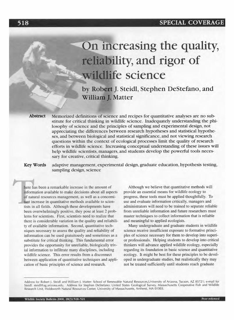
1- -reasing the quality, gor of
teidl, Stephen DeStefano, and
Abstraci nurszcu definitiu~lsul ~ L ~ C ~ I C Cand recipes for quantitative analyses are no sub-stitute for critical thinking in wildlife science. Inadequately understanding the phi-losophy of science and the principles of sampling and experimental design,not appreciating the differences between research hypotheses and statistical hypothe-ses,and between biological and statistical significance,and not viewing research questions within the context of ecological processes limit the quality of research efforts in wildlife science. Increasing conceptual understanding of these issues will help wildlife scientists,managers, and students develop the powerful tools neces-sary for creative,critical thinking.
Key Words adaptive management,experimental design,graduate education,hypothesis testing, sampling design,science
here has been a remarkable increase in the amount of information available to make decisions about all aspects of natural resources management, as well as a concomi-tant increase in quantitative methods available to scien-tists in all fields. Although these developments have been overwhelmingly positive, they pose at least 2 prob-lems for scientists. First, scientists need to realize that there is considerable variation in the quality and reliabili-ty of available information. Second, quantitative tech-niques necessary to assess the quality and reliability of information can be used gratuitously and sometimes as a substitute for critical thinking. This fundamental error provides the opportunity for unreliable, biologically triv-ial information to infiltrate many disciplines, including wildlife science. This error results from a disconnect between application of quantitative techniques and appli-cation of basic principles of science and research.
Although we believe that quantitative methods will provide an essential means for wildlife ecology to progress, these tools must be applied thoughtfully. To use and evaluate information critically, managers and administrators will need to be trained to separate reliable from unreliable information and future researchers must master techniques to collect information that is reliable and meaningful to applied ecologists.
Many undergraduate and graduate students in wildlife science receive insufficient exposure to formative princi-ples of science necessary for them to develop into superi-or professionals. Helping students to develop into critical thinkers will advance applied wildlife ecology, especially regarding its foundation in basic science and quantitative ecology. It might be best for these principles to be devel-oped in undergraduate studies, but realistically they may not be treated sufficiently until students reach graduate
Address for Robert j. Steidl and William J. Matter: School of Renewable Natural Resources,University of Arizona, Tucson, AZ 85721; e-mail for Steidl: [email protected]. Address for Stephen DeStefano: United States Geological Survey, Massachusetts Cooperative Fish and Wildlife Research Unit, Holdsworth Natural Resources Center, University of Massachusetts, Amherst, MA 01003.
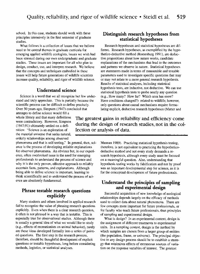
Quality, reliability, and rigor of wildlife science Steidl et al. 519
school. In this case, students should work with these Distinguish research hypotheses from principles intensively in the first semester of graduate studies. statistical hypotheses
What follows is a collection of issues that we believe need to be central themes in graduate curricula for emerging applied wildlife ecologists, issues we wish had been stressed during our own undergraduate and graduate studies. These issues are important for all who plan to design, conduct, use, and interpret research. We believe that the concepts and techniques embodied in these issues will help future generations of wildlife scientists increase quality, reliability, and rigor of wildlife science.
Understand science Science is a word that we all recognize but few under-
stand and truly appreciate. This is partially because the scientific process can be difficult to define precisely. Over 50 years ago, Simpson (1947) concluded that attempts to define science would fill a
Research hypotheses and statistical hypotheses are dif-ferent. Research hypotheses, as exemplified by the hypo-thetico-deductive method (Romesburg 1991), are deduc-tive propositions about how nature works, candidate explanations of the mechanisms that lead to the outcomes and patterns we observe in nature. Statistical hypotheses are statements made in terms of measurable and testable parameters used to investigate specific questions that may or may not relate to a more general research hypothesis. Results of statistical analyses, including statistical hypothesis tests, are inductive, not deductive. We can use statistical hypothesis tests to probe nearly any question (e.g., How many? How far? Which area has more? Have conditions changed?) related to wildlife; however, only questions about causal mechanisms require formu-lating explicit, deductive research hypotheses (Matter and
whole library and that many definitions were contradictory. However, Simpson (1947:91) ultimatelv settled on a defi-
The greatest gains in reliability and efficiency come during the design of research studies,not in the col-
nition: "Science is an exploration of lection or analysis of data. the material universe that seeks natural, orderly relationships among observed phenomena and that is self-testing." In general, then, sci- Mannan 1989). Practicing statistical hypothesis testing, ence is the process of developing reliable explanations therefore, is not equivalent to practicing the hypothetico-for observed phenomena. An obvious but, in our experi- deductive method and not every study demands a re-ence, often overlooked issue is the need for emerging search hypothesis, although every study must be focused professionals to understand the process of science and on a meaningful question. Also, understanding that why it is the only proven, effective approach to reliably hypothesis testing works by falsification and not by proof ascertain facts, patterns, and explanations. Although was an important developmental step for science, as it is being able to define science is important, learning to for the conceptual development of future professionals. think scientifically and to understand the process of sci-ence are absolutely fundamental.
Phrase testable research questions explicitly
Many students and others involved in applied research fail to recognize the value of phrasing research questions explicitly. Even when there is a clear research question, it often is not phrased in a way that is testable. This is especially true for observational studies. Although there is usually a general idea of what we would like to study (e.g., effects of recreationists on animal behavior), rarely are these ideas developed formally into a series of point-ed questions. The first step in the research process, therefore, should be thoughtful development of explicit questions or testable hypotheses, long before considering methods, logistics, or statistical analyses.
Understand the principles of sampling and experimental design
Successful acquisition of new knowledge of ecological relationships depends largely on the efficacy of methods used to collect data about natural phenomena. There are few concepts more important for future professionals, or for faculty who teach future professionals, than principles of sampling and experimental design.
What is design? In an experimental context, design is the assignment of different treatments to experimental units. In a sampling context, design is the method by which samples are chosen from a larger group of entities (the population, frame, or universe). The principal objec-tive in any design process should be to establish a strate-gy that minimizes effects of extraneous sources of varia-tion on the response variables of interest. The greatest
520 WiZdZije Society Bulletilz 2000,28(3):518-521
gains in reliability and efficiency come during the design of research studies, not in the collection or analysis of data. In fact, careful design can reduce the amount of field work necessary and will always simplify data analy- ses. Further, if a design is sound, an incorrect statistical analysis can always be redone; if a design is flawed, not even the most sophisticated statistical analysis will be able to resurrect it completely.
Undergraduate students have more opportunities than ever to experience the excitement of field and laboratory research. Given the many demands on undergraduate curricula, however, few can offer adequate treatment of the intricacies of sampling and research design. There- fore, every beginning graduate student should take a course in research design before they begin their re- search. In a short time, the payoff for students and for wildlife science would be apparent.
Focus on cause-and-effect and on experimental approaches
When possible, design studies in such a way that cau- sation (cause-and-effect) can be established. Experi- mentation, which by definition includes a manipulation induced by the researcher, is the only mechanism avail- able to establish genuine, direct causation, because it can eliminate the adverse effects of confounding variables. This is one of several powerful benefits of experimental studies over observational studies. Amassing observa- tional data about a phenomenon rarely allows us to estab- lish causation, and large correlation coefficients do not imply causation.
Further, we have heard ecologists of all ilks call repeatedly for increased experimentation, only to follow that call with the caveat that "well, experiments in ecolo- gy can be very difficult." We suggest that wildlife scien- tists need to be more creative. Certainly, we cannot always perform critical experiments, but we could do so far more often than we acknowledge. There is nearly always a way to manipulate, in a meaningful way, a sys- tem under study if enough thought and creative energy are targeted at that system.
Never perform a management manipulation unless it is part of an
adaptive management program We advocate the need, indeed the responsibility, for
wildlife scientists to establish monitoring programs to quantify results of management manipulations. Many of us have witnessed large-scale management manipulations
with no follow-up efforts to assess their effectiveness. These are tremendous opportunities to gain information that are lost due to poor planning and short-range think- ing. Management and monitoring must be linked inti- mately if we hope to increase our knowledge about the response of larger, complex systems to perturbations.
View research within the context of applied ecology, not as questions about
species Perhaps the greatest distinction between programs in
applied ecology, including wildlife science, and those in basic or "pure" ecology is the way we view research questions. When students are asked about what they study, those in wildlife science often reply with the name of the species that is the subject of their research. In contrast, students of basic ecology consider ecological relationships first. They focus on concepts such as forag- ing strategies and trophic interactions and mention the target species only as an afterthought. We all eventually collect the same kinds of data and use the same tech- niques, but we view our research and ultimate contribu- tions differently.
As superficial as this issue may seem, we believe that wildlife science would improve if we changed our view from species-centric to process-centric, Viewing research questions from the broader context of ecological process- es makes more obvious the contributions of all research efforts, including single-species studies, to the larger sciences of ecology and biology. When we view our re- search from a "species" perspective, we can easily over- look potential contributions beyond increased under- standing of species life-history characteristics.
Distinguish between biological and statistical significance
No statement is more meaningless than "population A was significantly different than population B." Because this verbiage is used so often, we may believe that it con- veys useful information. Actually, it provides evidence that we can become enamored with quantitative tools that appear objective but in reality are simply a poor replace- ment for critical thinking.
Virtually no 2 biological entities are identical, and even small, meaningless differences can be detected with large sample sizes and high precision of measurement. Wildlife scientists who contemplate debates about power analysis and the role of statistical hypothesis testing (Harlow et al. 1997, Steidl et al. 1997) realize that strict
Quality,reliability, and rigor of wildlife science Steidl et al.
hypothesis testing (i.e., testing that yields a dichotomous result: things are either different or they are not different) has been shunned by statisticians for many years because it provides so little useful information. The genuine question is whether 2 populations differ by a biologically meaningful quantity. Was the relative difference ob-served between populations 1% or 65%? Biological information is contained in the measurements we make, not in probabilistic statements about null hypotheses of zero effect. If these ideas are new to you, we suggest reading Johnson (1999), who provides a good overview of the relevant issues.
No scientific discipline is likely to abandon hypothesis testing anytime soon, or even should, but we believe that appropriate roles of hypothesis testing, estimation, and research design need to be better understood. We need to establish what constitutes a biologically meaningful differ-ence between groups, an act that requires careful and criti-cal thought. There will never be a simple, general solution to this necessary step. When we think about and report research results, we must do so regarding size of the bio-logical effects measured, rather than only P-values and test statistics; the latter should be viewed only as useful sup-portive information, relegated to parentheses. Our knowl-edge of ecology will be increased most by assessing the measurements we make, not by performing statistical tests.
Conclusions The bad news is that many students attracted to the
wildlife profession are not attracted by or excited about learning and using quantitative tools. The good news is that the greatest gains in research do not rely on mastery of mathematics, but rather rely on developing a better understanding of the concepts of experimental design and sampling design, scope of inference, establishing cause-and-effect, and the philosophy and processes of science. Further, most statistics and other quantitative tools, although often based on complex mathematics, are not dif-ficult to understand conceptually. Utilitarian understand-ing requires only that you realize how they work concep-tually and that this conceptual base gives you insights into interpretation. In the courses we teach, therefore, we encourage students to approach quantitative measures con-ceptually first rather than mathematically; we encourage
faculty to consider teaching these measures from a con-ceptual perspective. If students understand concepts, com-putations come more easily; the reverse rarely is true.
This incomplete list of issues and ideas that we pres-ent represents mistakes or oversights we have made our-selves. However, new professionals need not repeat these mistakes as part of rights-of-passage into the field of wildlife ecology. Further, we must address these issues at all levels in our profession. Administrators will need to understand these issues so they can recognize and fund quality proposals; managers will need to understand these issues so they can monitor the results of manage-ment manipulations; and researchers need to understand these issues so they can design studies with great preci-sion and reliability.
Acknowledgments. We appreciate the constructive comments provided by R. D. Brown and C. Boggis.
Literature cited HARLOW,L. L., S. A. MULWK,AND J. H. STEIGER.editors. 1997. What if
there were no significance tests? Lawrence Erlbaum and Associates,Mahwah, New Jersey, USA.
JOHNSON,D. H. 1999. The insignificance of statistical significance test-ing. Journal of Wildlife Management 63:763-772.
MATTER,W J., AND R. MAUUAS. 1989. More on gaining reliable knowledge-a comment. Journal of Wildlife ;Llanagement 53:1172-1176.
RO~IESB~RG,H. C . 1991. On improving the natural resources and envi-ronmental sciences. Jourilal of Wildlife Management 55:744-756.
SIMPSON,G. G. 1947. This view of life. Harcourt. Brace,and World,New York, New York, USA.
STEIDL,R. J., J. l? HAYES,AND E. SCHAL-BER.1997. Statisticalpower analy-sis in wildlife research. Journal of Wildlife Management 61:270-279.
Robert). Steidl is assistant professor of wildlife and fisheries sciences in the School of Renewable Natural Resources at the University of Arizona. Stephen DeStefano is unit leader and adjunct associate pro-fessor with the Massachusetts Cooperative Fish and Wildlife Research Unit and Department of Natural Resources Conservation, University of Massachusetts, Amherst. William 1. Matter is associate professor of wildlife and fisheries sciences and coordinator of undergraduate advis-ing and curricula in the School of Renewable Natural Resources at the University of Arizona.
Associate Editor: Krausman
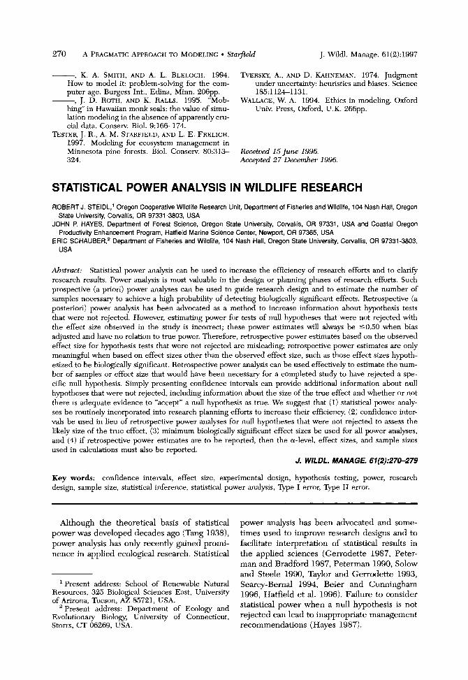
270 A PRAGMATICAPPROACHTO MODELINGStarfield J. Wildl. Manage. 61(2):1997
, K. A. SMITH, AND A. L. BLELOCH.1994. TvERSKY, A,, AND D. KAHNEMAN.1974. Judgment How to model it: problem-solving for the com- under uncertainty: heuristics and biases. Science puter age. Burgess Int., Edina, Minn. 206pp. 185:1124-1131.
, J. D. ROTH,AND K. RALLS. 1995. "Mob- WALLACE,W. A. 1994. Ethics in modeling. Oxford bing" in Hawaiian monk seals: the value of simu- Univ. Press, Oxford, U.K. 266pp. lation modeling in the absence of apparently cru-cial data. Conserv. Biol. 9:166-174.
TESTER,J. R., A. M. STARFIELD,AND L. E. FRELICH. 1997. Modeling for ecosystem management in Minnesota pine forests. Biol. Conserv. 80:313- Received 15 June 1996. 324. Accepted 2 7 December 1996.
STATISTICAL POWER ANALYSIS IN WILDLIFE RESEARCH
ROBERT J. STEIDL,' Oregon Cooperative Wildlife Research Unit, Department of Fisheries and Wildlife, 104 Nash Hall, Oregon State University, Cowallis, OR 97331-3803, USA
JOHN P. HAYES, Department of Forest Science, Oregon State University, Cowallis, OR 97331, USA and Coastal Oregon Productivity Enhancement Program, Hatfield Marine Science Center, Newport, OR 97365, USA
ERIC SCHAUBER,2Department of Fisheries and Wildlife, 104 Nash Hall, Oregon State University, Cowallis, OR 97331-3803, USA
Abstract: Statistical power analysis can be used to increase the efficiency of research efforts and to clarify research results. Power analysis is most valuable in the design or planning phases of research efforts. Such prospective (a priori) power analyses can be used to guide research design and to estimate the number of samples necessary to achieve a high probability of detecting biologically significant effects. Retrospective (a posteriori) power analysis has been advocated as a method to increase information about hypothesis tests that were not rejected. However, estimating power for tests of null hypotheses that were not rejected with the effect size observed in the study is incorrect; these power estimates will always be 50.50 when bias adjusted and have no relation to true power. Therefore, retrospective power estimates based on the observed effect size for hypothesis tests that were not rejected are misleading; retrospective power estimates are only meaningful when based on effect sizes other than the observed effect size, such as those effect sizes hypoth-esized to be biologcally significant. Retrospective power analysis can be used effectively to estimate the num-ber of samples or effect size that would have been necessary for a completed study to have rejected a spe-cific null hypothesis. Simply presenting confidence intervals can provide addtional information about null hypotheses that were not rejected, including information about the size of the true effect and whether or not there is adequate evidence to "accept" a null hypothesis as true. We suggest that (1)statistical power analy-ses be routinely incorporated into research planning efforts to increase their efficiency, (2) confidence inter-vals be used in lieu of retrospective power analyses for null hypotheses that were not rejected to assess the likely size of the true effect, (3) minimum biologically significant effect sizes be used for all power analyses, and (4) if retrospective power estimates are to be reported, then the a-level, effect sizes, and sample sizes used in calculations must also be reported.
J. WILDL. MANAGE. 61(2):27&279
Key words: confidence intervals, effect size, experimental design, hypothesis testing, power, research design, sample size, statistical inference, statistical power analysis, Type I error, Type I1 error.
Although the theoretical basis of statistical power was developed decades ago (Tang 1938), power analysis has only recently gained promi-nence in applied ecological research. Statistical
'Present address: School of Renewable Natural Resources, 325 Biological Sciences East, University of Arizona, Tucson, AZ 85721, USA.
" Present address: Department of Ecology and Evolutionary Biology, University of Connecticut, Storrs, CT 06269, USA.
power analysis has been advocated and some-times used to improve research designs and to facilitate interpretation of statistical results in the applied sciences (Gerrodette 1987, Peter-man and Bradford 1987, Peterman 1990, Solow and Steele 1990, Taylor and Gerrodette 1993, Searcy-Bernal 1994, Beier and Cunningham 1996. Hatfield e t al. 1996). Failure to consider statistical power when a null hypothesis is not rejected can lead to inappropriate management recommendations (Hayes 1987).
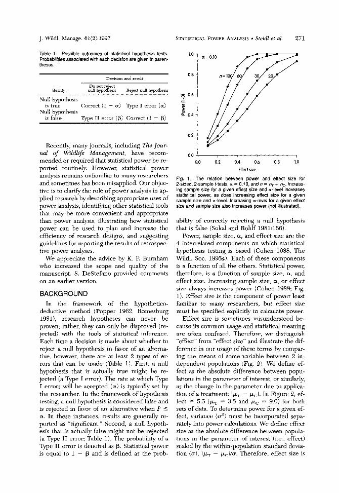
J. Wildl. Manage. 61(2):1997 STATISTICALPOWERANALYSIS Steidl et al. 271
Table 1. Possible outcomes of statistical hypothesis tests. Probabilitiesassociated with each decision are given in paren-theses.
Decision and result
Do not re'ect Reality null hypotiesis Reject null hypothesis
Null hypothesis is true Correct (1 - a) Type I error (a)
Null hypothesis is false Type I1 error (P) Correct (1 - P)
Recently, many journals, including The Jour-nal of Wildlqe Management, have recom-mended or required that statistical power be re-ported routinely. However, statistical power analysis remains unfamiliar to many researchers and sometimes has been misapplied. Our objec-tive is to clarify the role of power analysis in ap-lied research by describing appropriate uses of
power analysis, identifying other statistical tools that may be more convenient and appropriate than power analysis, illustrating how statistical power can be used to plan and increase the efficiency of research designs, and suggesting guidelines for reporting the results of retrospec-tive power analyses.
We appreciate the advice by K. P. Burnham who increased the scope and quality of the manuscript. S. DeStefano provided comments on an earlier version.
BACKGROUND In the framework of the hypothetico-
deductive method (Popper 1962, Romesburg 1981), research hypotheses can never be proven; rather, they can only be disproved (re-jected) with the tools of statistical inference. Each time a decision is made about whether to reject a null hypothesis in favor of an alterna-tive, however, there are at least 2 types of er-rors that can be made (Table 1).First, a null hypothesis that is actually true might be re-jected (a Type I error). The rate at which Type I errors will be accepted (a)is typically set by the researcher. In the framework of hypothesis testing, a null hypothesis is considered false and is rejected in favor of an alternative when P 5 a . In these instances, results are generally re-ported as "significant." Second, a null hypoth-esis that is actually false might not be rejected (a Type I1 error; Table 1). The probability of a Type I1 error is denoted as P. Statistical power is equal to 1 - P and is defined as the prob-
0.00, 0.0 0.2 0.4 0.6 0.8 1.0
Effect size
Fig. 1. The relation between power and effect size for 2-sided, 2-sample t-tests, cx = 0.10, and n = n, + n,. Increas-ing sample size for a given effect size and a-level increases statistical power, as does increasing effect size for a given sample size and a-level. Increasing a-level for a given effect size and sample size also increases power (not illustrated).
ability of correctly rejecting a null hypothesis that is false (Sokal and Rohlf 1981:166).
Power, sample size, a,and effect size are the 4 interrelated components on which statistical hypothesis testing is based (Cohen 1988, The Wildl. Soc. 1995~) .Each of these components is a function of all the others. Statistical power, therefore, is a function of sample size, a, and effect size. Increasing sample size, a, or effect size always increases power (Cohen 1988; Fig. 1).Effect size is the component of power least familiar to many researchers, but effect size must be specified explicitly to calculate power.
Effect size is sometimes misunderstood be-cause its common usage and statistical meaning are often confused. Therefore, we dstinguish "effect" from "effect size" and illustrate the dif-ference in our usage of these terms by compar-ing the means of some variable between 2 in-dependent populations (Fig. 2 ) . We define ef-fect as the absolute difference between popu-lations in the parameter of interest, or similarly, as the change in the parameter due to applica-tion of a treatment: Ik - kcIIn Figure 2, ef-fect = 5.5 (k= 3.5 and kc = 9.0) for both sets of data. To determine power for a given ef-fect, variance (u2)must be incorporated sepa-rately into power calculations. We define effect size as the absolute difference between popula-tions in the parameter of interest (i.e.,effect) scaled by the within-population standard devia-tion (a),l k - p,Ci/u. Therefore, effect size is
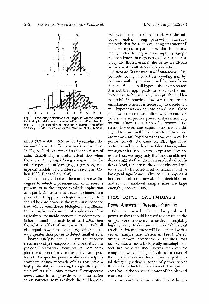
272 STATISTIC~LPOWERANALYSIS Steidl et al. J. U'ildl. Manage. 61(2):1997
Fig. 2. Frequency distributions for 2 hypothetical populations illustrating the differences between effect and effect size. Ef-fect (pT- pCI)is identical for both sets of distributions; effect size (p, - ~ C l / ~ )is smaller for the lower set of distributions.
effect (3.5 - 9.0 = 5.5) scaled by standard de-viation (if o = 2.0, effect size = 5.5/2.0 = 2.75). In Figure 2, effect size differs for the 2 sets of data. Establishing a useful effect size when there are >2 groups being compared or for other types of analyses (e.g., regression, cat-egorical models) is considered elsewhere (Co-hen 1988, Richardson 1996).
Conceptually, effect can be considered as the degree to which a phenomenon of interest is present, or as the degree to which application of a particular treatment causes a change in a parameter. In applied ecological research, effect should be considered as the minimum response that will be considered biologically significant. For example, to determine if application of an agricultural pesticide reduces a resident popu-lation of small mammals by at least 20%, then the relative effect of interest is 20%. With all else equal, power to detect large effects is al-ways greater than power to detect small effects.
Power analysis can be used to improve research design (prospective or a priori) and to provide information about results from com-pleted research efforts (retrospective or a pos-teriori). Prospective power analysis can help re-searchers design research efforts that have a high probability of detecting biologically signifi-cant effects (i.e., high power). Retrospective power analysis can provide some information about statistical tests in which the null hypoth-
esis was not rejected. Although we illustrate power analysis using parametric statistical methods that focus on evaluating treatment ef-fects (changes in parameters due to a treat-ment) under the requisite assumptions (sample independence, homogeneity of variance, nor-mally distributed errors), the issues we discuss are relevant to all statistical approaches.
A note on 'accepting" null hypotheses.-Hy-pothesis testing is based on rejecting null hy-potheses with a predetermined degree of con-fidence. When a null hypothesis is not rejected, it is not then appropriate to conclude the null hypothesis to be true (i.e.,"accept" the null hy-pothesis). In practice, however, there are cir-cumstances when it is necessary to decide if a null hypothesis can be considered true. These practical concerns are often why researchers perform retrospective power analyses, and why journal editors request they be reported. We stress, however, that experiments are not de-signed to prove null hypotheses true; therefore, accepting a null hypothesis as true can never be performed with the same scientific rigor as re-jecting a null hypothesis as false. Hence, when we suggest it reasonable to accept a null hypoth-esis as true, we imply only that the available evi-dence suggests that, given an established confi-dence level, the size of the effect observed was too small to be considered of management or biological significance. This point is important because an effect of any size is detectable-no matter how small-if sample sizes are large enough (Johnson 1995).
PROSPECTIVE POWER ANALYSIS
Power Analysis in Research Planning When a research effort is being planned,
power analysis should be used to determine the sample sizes necessary to achieve acceptably high power, or to determine the probability that an effect size of interest will be detected with a certain sample size (Peterman 1990). Deter-mining power prospectively requires that sample size, a, and a biologically meaningful ef-fect size be established. Power then can be computed with a range of values for each of these parameters and for different experimen-tal designs, yielding a series of power curves that indicate the influence each of these param-eters has on the statistical power of the planned research effort.
To use power analysis, a study must be de-
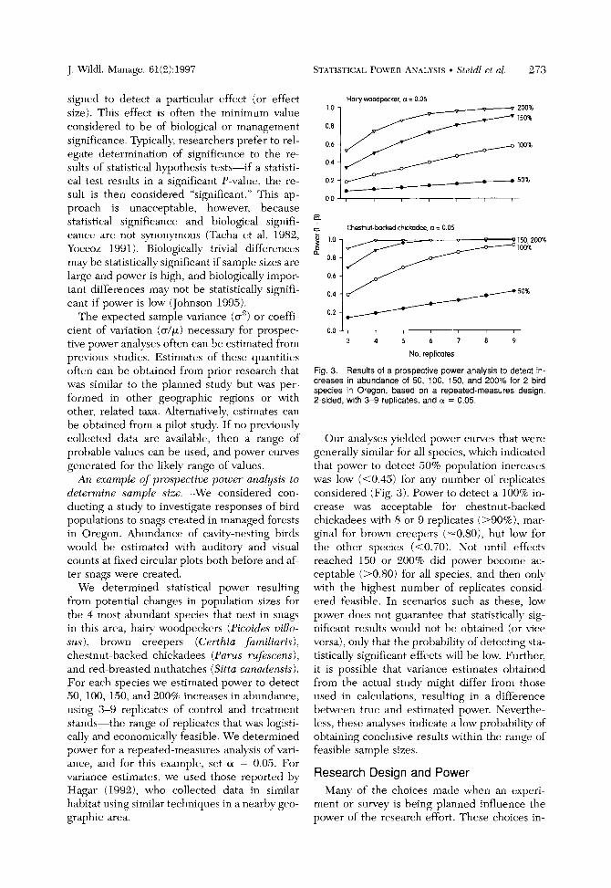
J. LYildl. hlanage.61(2):1997 STATISTICALPOWERASALYSIS Steicll et al. 273
signed to detect a particular effect (or effect size). This effect is often the minimurn value considered to be of biological or management significance. Typically, researchers prefer to rel-egate determination of significance to the re-sults of statistical hypothesis tests-if a statisti-cal test results in a significant P-value, the re-sult is then considered "significant." This ap-proach is unacceptable, however, because statistical significance and biological signifi-cance are not synonymous (Tacha et al. 1982, Yoccoz 1991). Biologically trivial differences may be statistically significant if sample sizes are large and power is high, and biologically impor-tant differences may not be statistically signifi-cant if power is low (Johnson 1995).
The expected sample variance (u') or coeffi-cient of variation (u/p)necessary for prospec-tive power analyses often can be estimated from pre~iousstudies. Estimates of these quantities often can be obtained from prior research that was similar to the planned study but was per-formed in other geographic regions or with other, related taxa. Alternatively, estimates can be obtained from a pilot study. If no previously collected data are available, then a range of probable values can be used, and power cun7es generated for the likely range of values.
An eman~pleofpro.spectiue potccr analysis to determine .sample size.-\Ve considered con-ducting a study to investigate responses of bird populations to snags created in managed forests in Oregon. Abundance of ca~iv-nestingbirds \vould he estimated with auditory and ~ i sua l counts at fixed circular plots both before and af-ter snags were created.
\Ye determined statistical power resulting from potential changes in population sizes for the 3 most abundant species that nest in snags in this area, ha in woodpeckers (Picoides cillo-su ,s ) , brown creepers (Certhia fan~iliar-is), chestnut-backed chickadees (Parus i'ufescens), and red-breasted nuthatches (Sitta canadensis). For each species we estimated power to detect 50, 100, 1.30,and 200% increases in abundance, using :3-9 replicates of control and treatment stands-the range of replicates that was logisti-cally and economically feasible. \f7e determined power for a repeated-measures analysis of'vari-ance, and for this example, set a = 0.05. For variance estimates, we used those reported by I-Iagar (1992), m~hocollected data in sirnilar habitat using sinlilar techniques in a nearby geo-graphic area.
Haiw woodwcker. a = 0.05
3 Chestnut-backedchickadee,a= 0 05
0 0 I ,
3 4 5 6 7 8 9
No, replicates
Fig. 3. Results of a prospective power analysis to detect in-creases in abundance of 50, 100, 150, and 200% for 2 bird species in Oregon, based on a repeated-measures design, 2-sided, with 3-9 replicates, and a = 0.05.
Our analyses yielded power curves that were generally sirnilar for all species, which indicated that power to detect 50% population increases was lo\v (<0.45) for any number of replicates considered (Fig.3 ) .Power to detect a 100% in-crease \vas acceptable for chestnut-backed chickadees with 8 or 9 replicates (>go%), mar-ginal for brown creepers (-=0.80),but lo~vf i~ r the other species (<O.'iO). Not until effects reached 130 or 200% did power become ac-ceptable (>0.80) for all species, and then only with the highest number of replicates consid-ered feasible. In scenarios such as these, low power does not guarantee that statisticall>-sig-nificant results would not be obtained (or \ice versa),only that the probability of detecting sta-tisticalll- significant effects will be low. Further. it is possible that variance estimates ot~tainecl fro111 the actual study might differ from those used in calculations, resulting in a difference between true and estimated power. Neverthe-less, these analyses indicate a low probability of obtaining conclusive results within the range of feasible sample sizes.
Research Design and Power Many of the choices made when an experi-
ment or sune! is being planned influence the power of the research effort. These choices in-
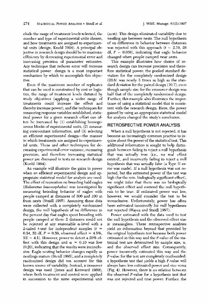
274 STATISTICALPOWERANALYSIS Steidl et al. J. Wildl. Manage. 61(2):1997
clude the range of treatment levels selected, the number and type of experimental units chosen, and how treatments are assigned to experimen-tal units (design; Kuehl 1994).A principal ob-jective in research design should be to maximize efficiency by decreasing experimental error and increasing precision of parameter estimates. Any technique that reduces error will increase statistical power-design is a most important mechanism by which to accomplish this objec-tive.
Even if the maximum number of replicates that can be used is constrained by cost or logis-tics, the range of treatment levels &ctated by study objectives (applying a wider range of treatments could increase the effect and thereby increase power), and the techniques for measuring response variables established, statis-tical power for a given research effort can of-ten be increased by (1)establishing homoge-neous blocks of experimental units, (2) measur-ing concomitant information, and (3) selecting an efficient experimental design-the manner in which treatments are assigned to experimen-tal units. These and other techniques for de-creasing experimental error variance, increasing precision, and therefore increasing statistical power are discussed in texts on research design (Kuehl 1994).
An example will illustrate the gains in power when an efficient experimental design and ap-propriate statistical model for analysis are used. The effect of recreation on breedng bald eagles (Haliaeetus leucocephalus) was investigated by measuring brooding behavior of eagles with people camped at &stances of 500 and 100 m from nests (Steidl 1995). Assuming these data were collected with a completely randomized design, the null hypothesis of no difference in the percent day that eagles spent brooding with people camped at these 2 distances could not be rejected at any reasonable a-level with a %tailed t-test for independent samples (t =
0.54, 52 df, P = 0.59, observed effect = 4.5%, SE = 4.1). However, power to detect a 20% ef-fect with this design and a = 0.10 was low (0.20),indicating that the results were inconclu-sive. Eagle nesting behavior changes rapidly as nestlings mature (Steidl1995),and a completely randomized design did not account for this known source of variability. Instead, a crossover design was used (Jones and Kenward 1989), where both treatment and control were applied in succession to the same experimental unit
(nest).This design eliminated variability due to nestling age between nests. The null hypothesis of no difference in behavior between &stances was rejected with this approach (t = 2.19, 26 df, P = 0.038), indicating that eagle behavior changed when people camped near nests.
This example illustrates how choice of re-search design can increase precision and there-fore statistical power: the pooled standard de-viation for the completely randomized design (29.8) was nearly 3 times as high as the stan-dard deviation for the paired design (10.7),even though sample size for the crossover design was half that of the completely randomized design. Further, this example also illustrates the impor-tance of using a statistical model that is consis-tent with the research design. Here, the power gained by using an appropriate statistical model for analysis changed the study's conclusion.
RETROSPECTIVE POWER ANALYSIS When a null hypothesis is not rejected, it has
become an increasingly common practice to in-quire about the power of the statistical test. This additional information is sought to help &stin-guish between failing to reject a null hypothesis that was actually true (i.e., no real effect existed), and incorrectly failing to reject a null hypothesis that was actually false (a Type 11 er-ror was made). If a null hypothesis was not re-jected, but the estimated power of the test was high (for the min. biologically significant effect), we might infer that there was no biologically significant effect and contend the null hypoth-esis to be true. If estimated power was low, however, we would consider the test to be inconclusive. Unfortunately, power has often been estimated incorrectly for null hypotheses not rejected (Hayes and Steidl 1997).
Power estimated with the data used to test the null hypothesis and the observed effect size is meaningless. These retrospective analyses yield no information beyond that provided by the original hypothesis test because both power estimated in this way and the P-value of the sta-tistical test are determined by sample size, a, and the observed effect size. Consequently, power incorrectly estimated this way and the P-value for the test are completely confounded: a hypothesis test that yields a high P-value will always have low estimated power and vice versa (Fig. 4). However, there is no relation between the observed P-value for a hypothesis test that was not rejected and true power. Further, the
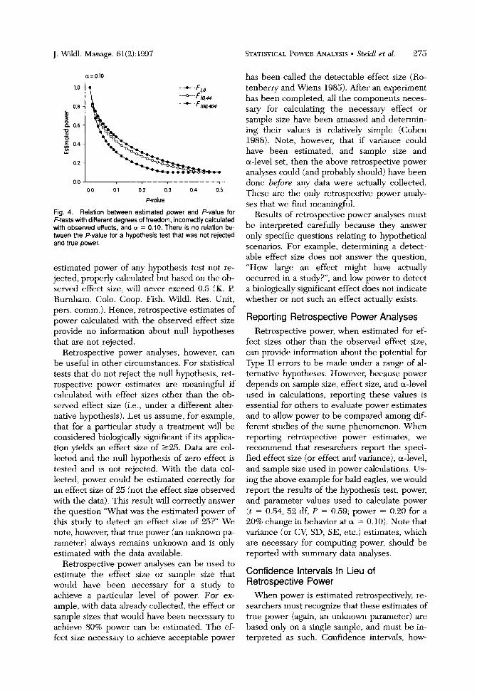
J. Wildl. Manage. 61(2):1997
Fig. 4. Relation between estimated power and P-value for F-testswith different degreesof freedom, incorrectlycalculated with observed effects, and a = 0.10. There is no relation be-tween the P-value for a hypothesis test that was not rejected and true power.
estimated power of any hypothesis test not re-jected, properly calculated but based on the ob-served effect size, will never exceed 0.5 (K. P. Burnham, Colo. Coop. Fish. Wildl. Res. Unit, pers. comm.).Hence, retrospective estimates of power calculated with the observed effect size provide no information about null hypotheses that are not rejected.
Retrospective power analyses, however, can be useful in other circumstances. For statistical tests that do not reject the null hypothesis, ret-rospective power estimates are meaningful if calculated with effect sizes other than the ob-served effect size (i.e., under a different alter-native hypothesis). Let us assume, for example, that for a particular study a treatment will be considered biologically significant if its applica-tion yields an effect size of 225. Data are col-lected and the null hypothesis of zero effect is tested and is not rejected. With the data col-lected, power could be estimated correctly for an effect size of 25 (not the effect size observed with the data). This result will correctly answer the question "What was the estimated power of this study to detect an effect size of 25?" We note, however, that true power (an unknown pa-rameter) always remains unknown and is only estimated with the data available.
Retrospective power analyses can be used to estimate the effect size or sample size that would have been necessary for a study to achieve a particular level of power. For ex-ample, with data already collected, the effect or sample sizes that would have been necessary to achieve 80% power can be estimated. The ef-fect size necessary to achieve acceptable power
STATISTICAL POWERANALYSIS Steidl et al. 275
has been called the detectable effect size (Ro-tenberry and Wiens 1985).After an experiment has been completed, all the components neces-sary for calculating the necessary effect or sample size have been amassed and determin-ing their values is relatively simple (Cohen 1988). Note, however, that if variance could have been estimated, and sample size and a-level set, then the above retrospective power analyses could (and probably should) have been done before any data were actually collected. These are the only retrospective power analy-ses that we find meaningful.
Results of retrospective power analyses must be interpreted carefully because they answer only specific questions relating to hypothetical scenarios. For example, determining a detect-able effect size does not answer the question, "How large an effect might have actually occurred in a study?", and low power to detect a biologically significant effect does not indicate whether or not such an effect actually exists.
Reporting Retrospective Power Analyses Retrospective power, when estimated for ef-
fect sizes other than the observed effect size, can provide information about the potential for Type I1 errors to be made under a range of al-ternative hypotheses. However, because power depends on sample size, effect size, and a-level used in calculations, reporting these values is essential for others to evaluate power estimates and to allow power to be compared among dif-ferent studies of the same phenomenon. When reporting retrospective power estimates, we recommend that researchers report the speci-fied effect size (or effect and variance), a-level, and sample size used in power calculations. Us-ing the above example for bald eagles, we would report the results of the hypothesis test, power, and parameter values used to calculate power ( t = 0.54, 52 df, P = 0.59; power = 0.20 for a 20% change in behavior at a = 0.10). Note that variance (or C\r, SD, SE, etc.) estimates, which are necessary for computing power, should be reported with summary data analyses.
Confidence Intervals In Lieu of Retrospective Power
When power is estimated retrospectively, re-searchers must recognize that these estimates of true power (again, an unknown parameter) are based only on a single sample, and must be in-terpreted as such. Confidence intervals, how-
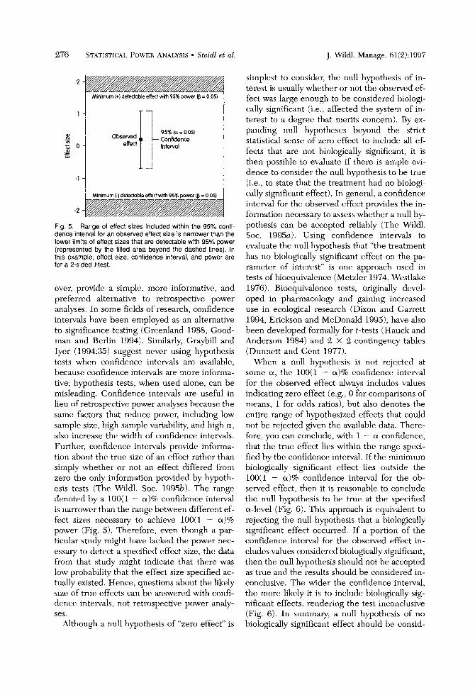
276 STATISTICAI,POWERANALYSISSteidl et al. J. Wildl. Manage. 61(2).1997
simplest to consider, the null hypothesis of in-terest is usually whether or not the observed ef-
M~n~mum(+Idetedoble effect w~th95% power IP = o 051 fect was large enough to be considered biologi-cally significant (i.e.,affected the system of in-terest to a degree that merits concern). By ex-panding null hypotheses beyond the strict statistical sense of zero effect to include all ef-fects that are not biologically significant, it is then possible to evaluate if there is arnple evi-dence to consider the null hypothesis to be true
-1 (i.e.,to state that the treatment had no biologi-M nmLm -I delectaole efled w,th 95% power la = 0 051d c,ill!. sip,nit>cantc1f'fcc.t1. In ycnc.r,tl. u co~~ticlt.~lcc
7-7 7-,@"/"7,7--7-. intrn.ad h r t11eo\)sc.n.t.tl effect l)ro\idcs t11(.in-' ' 4 ti,rm~itionnrc,c-ssnn.to ,issc3ss \\.I~ctl~el-a null I ) \ . -
Fig. 5. Range of effect sizes included within the 95% confi-dence interval for an observed effect size is narrower than the lower limits of effect sizes that are detectable with 95% power (represented by the filled area beyond the dashed lines). In this example, effect size, confidence interval, and power are for a 2-sided t-test.
ever, provide a simple, more informative, and preferred alternative to retrospective power analyses. In some fields of research, confidence intervals have been employed as an alternative to significance testing (Greenland 1988, Good-man and Berlin 1994). Similarly, Graybill and Iyer (1994:35) suggest never using hypothesis tests when confidence intervals are available, because confidence intervals are more informa-tive; hypothesis tests, when used alone, can be misleading. Confidence intervals are useful in lieu of retrospective power analyses because the same factors that reduce power, including low sample size, high sample variability, and high a, also increase the width of confidence intervals. Further, confidence intervals provide informa-tion about the true size of an effect rather than simply whether or not an effect differed from zero the only information provided by hypoth-esis tests (The Wildl. Soc. 1995b). The range denoted by a 100(1 - a ) % confidence interval is narrower than the range between different ef-fect sizes necessary to achieve l O O ( 1 - a)% power (Fig. 5).Therefore, even though a par-ticular study might have lacked the power nec-essary to detect a specified effect size, the data from that study might indicate that there was low probability that the effect size specified ac-tually existed. Hence, questions about the likely size of true effects can be answered with confi-dence intervals, not retrospective power analy-ses.
Although a null hypothesis of "zero effect" is
pothesis can be accepted reliably (The ~ i l d l . Soc. 1995~) .Using confidence intervals to evaluate the null hypothesis that "the treatment has no biologically significant effect on the pa-rameter of interest" is one approach used in tests of bioequivalence (Metzler 1974,Westlake 1976). Bioequivalence tests, originally devel-oped in pharmacology and gaining increased use in ecological research (Dixon and Garrett 1994, Erickson and McDonald 1995),have also been developed formally for t-tests (Hauck and Anderson 1984) and 2 X 2 contingency tables (Dunnett and Gent 1977).
When a null hypothesis is not rejected at some a, the 100(1 - a)% confidence interval for the observed effect always includes values indicating zero effect (e.g.,O for comparisons of means, 1for odds ratios), but also denotes the entire range of hypothesized effects that could not be rejected given the available data. There-fore, you can conclude, with 1 - a confidence, that the true effect lies within the range speci-fied by the confidence interval. If the minimum biologically significant effect lies outside the 100(1 - a ) % confidence interval for the ob-served effect, then it is reasonable to conclude the null hypothesis to be true at the specified a-level (Fig. 6). This approach is equivalent to rejecting the null hypothesis that a biologically significant effect occurred. If a portion of the confidence interval for the observed effect in-cludes values considered biologically significant, then the null hypothesis should not be accepted as true and the results should be considered in-conclusive. The wider the confidence interval, the more likely it is to include biologically sig-nificant effects, rendering the test inconclusive (Fig. 6). In summary, a null hypothesis of no biologically significant effect should be consid-
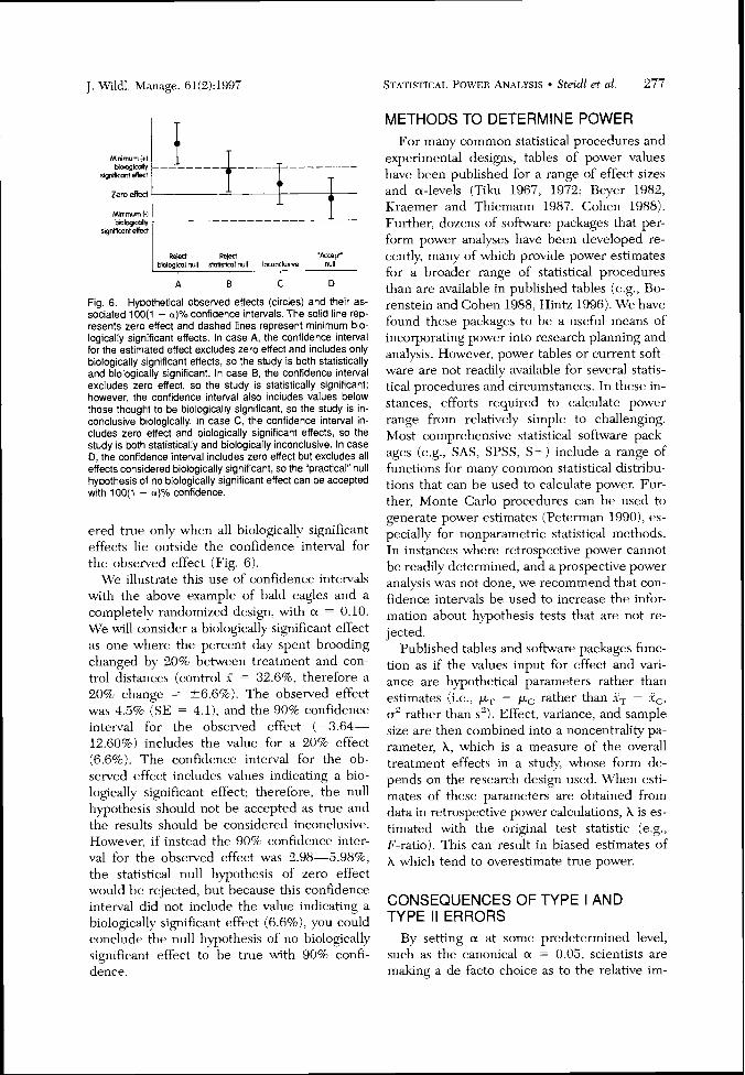
J . \%'ildl. Manage. 61(2):1997 STATISTICALPO\VERANALYSIS Steidl et al. 277
Mlnlmum 1+1
s8gnlRcanteffect
Zero effed
Reled Reject 'accept' bmlogicalnull M M c a lnull lnconclusne null
A B C D
Fig. 6. Hypothetical observed effects (circles) and their as-sociated 100(1 - a)% confidence intervals. The solid line rep-resents zero effect and dashed lines represent minimum bio-logically significant effects. In case A, the confidence interval for the estimated effect excludes zero effect and includes only biologically significant effects, so the study is both statistically and biologically significant. In case B, the confidence interval excludes zero effect, so the study is statistically significant; however, the confidence interval also includes values below those thought to be biologically significant, so the study is in-conclusive biologically. In case C, the confidence interval in-cludes zero effect and biologically significant effects, so the study is both statistically and biologically inconclusive. In case D, the confidence interval includes zero effect but excludes all effects considered biologically significant, so the "practical" null hypothesis of no biologically significant effect can be accepted with 100(1 - a)% confidence.
ered true only when all biologically significant effects lie outside the confidence interval for the observed effect (Fig. 6).
\Ve illustrate this use of confidence intervals with the above example of bald eagles and a completely randornized design, with a = 0.10. \Ye mill consider a biologically significant effect as one where the percent day spent brooding changed by 20% behveen treatment and con-trol distances (control .i: = 32.6%, therefore a 20% change = 26.6%). The observed effect was 4.5% (SE = 4.11, and the 90% confidence intenal for the observed effect (-3.64-12.60%) includes the value for a 20% effect 16.6%). The confidence interval for the ob-sened effect includes values indicating a bio-logically significant effect; therefore, the null hyothesis should not be accepted as true and the results should be considered inconclusive. However, if instead the 90% confidence inter-\,a1 for the obsened effect was 2.98-5.98%, the statistical null hypothesis of zero effect would be rejected, but because this confidence in t end did not include the value indicating a biologically significant effect (6.6%),you could conclude the null hy~othesisof no biologically significant effect to be true with 90% confi-dence.
METHODS TO DETERMINE POWER For many common statistical procedures and
experimental designs, tables of power values have been published for a range of effect sizes and a-levels (Tiku 1967, 1972; Beyer 1982, Kraemer and Thiemann 1987, Cohen 1988). Further, dozens of software packages that per-form power analyses have been developed re-cently, many of which provide power estimates for a broader range of statistical procedures than are available in published tables (e.g., Bo-renstein and Cohen 1988, Hintz 1996).We have found these packages to be a useful means of incorporating power into research planning and analysis. However, power tables or current soft-ware are not readily available for several statis-tical procedures and circumstances. In these in-stances, efforts required to calculate power range from relatively simple to challenging. Most comprehensive statistical software pack-ages (e.g., SAS, SPSS, S + ) include a range of functions for many common statistical distribu-tions that can be used to calculate power. Fur-ther, Monte Carlo procedures can be used to generate power estimates (Peterman 1990),es-pecially for nonparametric statistical methods. In instances where retrospective power cannot be readily determined, and a prospective power analysis was not done, we recommend that con-fidence intervals be used to increase the infor-mation about hypothesis tests that are not re-jected.
Published tables and software packages func-tion as if the values input for effect and vari-ance are hypothetical parameters rather than estimates (i.e., pT - pc rather than .i:, - f,, a" rather than s'). Effect, variance, and sample size are then combined into a noncentrality pa-rameter, A, which is a measure of the overall treatment effects in a study, whose form de-pends on the research design used. When esti-mates of these parameters are obtained from data in retrospective power calculations, h is es-timated with the original test statistic (e.g., F-ratio). This can result in biased estimates of A which tend to overestimate true power.
CONSEQUENCES OF TYPE I AND TYPE ll ERRORS
By setting a at some predetermined level, such as the canonical a = 0.05, scientists are making a de facto choice as to the relative im-
278 STATISTICALPOWERANALYSIS Steid et al. J. Wild. Manage. 61(2):1997
portance of Type I and Type I1 errors, because p increases as a is reduced. Decreasing a can increase p to an unacceptably high level and consequently reduce power to an unacceptably low level. In many circumstances, such as when the costs of environmental effects could be great, the potential risks and consequences as-sociated with making a Type I1 error may out-weigh those associated with Type I errors (Toft and Shea 1983, Hayes 1987, Peterman 1990).
The burden of proof is typically on research-ers to "prove" a phenomenon exists by reject-ing the null hypothesis that the phenomenon does not exist. This approach implies a willing-ness to accept the consequences of Type I1 er-rors over those of Type I errors. In some situa-tions this approach may be appropriate. How-ever, when there are considerable risks associ-ated with management actions based on the results of hypothesis tests that are not rejected, the consequences of Type I1 errors can exceed those of Type I errors (Peterman 1990).For ex-ample, in the Pacific Northwest, there is a ques-tion as to the amount of timber that can be har-vested without adverse effects on songbird populations. A relevant null hypothesis might be that a particular level of timber harvest has no effect on the density of songbird populations. In this and similar instances, the null hypoth-esis might be stated as one of no effect. If an experiment with low statistical power is per-formed to test this hypothesis, the probability of rejecting the null hypothesis will be low, whether or not the true effect was biologically significant. If songbird populations were ad-versely affected by a certain level of timber har-vest, but forests continued to be managed as if songbirds were not affected because of deci-sions based on low-power tests, then this Type 11 error could lead to population declines.
Management actions resulting from hypoth-esis tests that were not rejected have an under-lying, often unrecognized, assumption about the relative costs of Type I and Type I1 errors that is independent of their true costs (Toft and Shea 1983, Cohen 1988, Peterman 1990).In particu-lar, when p 2 a,scientists implicitly assume that costs of Type I errors exceed those of Type 11 errors when their recommendations assume that a null hypothesis that is not rejected is true (Toft and Shea 1983). One approach suggests considering Type I1 errors as paramount when a decision would result in the loss of unique habitats or species (Shrader-Frechette and Mc-
Coy 1993). Other approaches have been sug-gested by which Type I and I1 errors can be bal-anced based on their relative costs (Osenberg et al. 1994).
In general, the framework of hypothesis test-ing has been largely overused by scientists (Sals-burg 1985, Yoccoz 1991), especially in the con-text of environmental decision making. Hypoth-esis tests only assess "statistical significance"; "practical importance" may be better evaluated by the use of confidence intervals (Graybill and Iyer 1994:xiii). Reliance on hypothesis testing should be decreased in favor of more informa-tive methods that better evaluate available in-formation, includng Bayesian methods (Ellison 1996). In circumstances similar to those out-lined above for timber and songbirds, the rel-evant issue is not whether timber harvest affects songbirds (obviously, there will be an effect on resident songbirds if all timber is cut); rather, the issue is to understand the magnitude of the effect caused by a particular level of harvest. Hypothesis testing should not be the only tool used for decision-making issues, especially where the risk associated with a decision is con-siderable. In these instances, knowledge of the potential risks and available evidence for each possible decision should guide the decision-making progress.
LITERATURE CITED BEIER,P., AND S. C. CUNNINGHAM.1996. Power of
track surveys to detect changes in cougar popu-lations. Wild. Soc. Bull. 24:540-546.
B E Y E ~W. H. 1982. CRC handbook of tables for probability and statistics. Chem. Rubber Co., Cleveland, Oh. 656pp.
BORENSTEIN,M., AND J. COHEN.1988. Statistical power analysis. Lawrence Erlbaum Assoc., Hills-dale, N.J. 187pp.
COHEN,J. 1988. Statistical power analysis for the behavioral sciences. Second ed. Lawrence Erl-baum Assoc., Hillsdale, N.J. 567pp.
DUN NET^, C. W., AND M. GENT. 1977. Significance testing to establish equivalence between treat-ments with special reference to data in the form of 2 X 2 tables. Biometries 33:593402.
DIXON,P. M., AND K. A. GARREIT.1994. Statistical issues for field experimenters. Pages 439450 in R. J. Kendall and T. E. Lacher, Jr., eds. Wildlife toxicology and population modeling: integrated studies of agroecosystems. CRC Press, Boca Raton, Fla.
ELLISON,A. M. 1996. An introduction to Bayesian inference for ecological research and environ-mental decision-making. Ecol. Appl. 6:103& 1046.
ERICKSON,W. P., AND L. L. MCDONALD.1995.
J. Wildl. Manage. 61(2):1997 STATISTICALPOWERANALYSISSteidl et al. 279
Tests for bioequivalence of control media and test media in studies of toxicity. Environ. Toxi-col. Chem. 14:1247-1256.
GERRODETTE,T. 1987. A power analysis for detect-ing trends. Ecology 68:13641372.
GOODMAN,S. N., AND J. A. BERLIN.1994. The use of predicted confidence intervals when planning experiments and the misuse of power when in-terpreting results. Annu. Intern. Med. 121:200-206.
GRAYBILL,F. A,, AND H. K. IYER 1994. Regression analysis: concepts and applications. Duxbury Press, Belmont, Calif. 701pp.
GREENLAND,S. 1988. On sample-size and power calculations for studies using confidence inter-vals. Am. J. Epidemiol. 128:231-237.
HAGARJ. C. 1992. Bird communities in commer-cially thinned and unthinned Douglas-fir stands of western Oregon. M.S. Thesis, Oregon State Univ., Corvallis. 1lOpp.
HATFIELD,J. S.,W. R. GOULD,B. A. HOOVER,M. R. FULLER,AND E. L. LINDQUIST.1996. Detect-ing trends in raptor counts: power and Type I error rates of various statistical tests. Wild. Soc. Bull. 24:505-515.
HAUCK,W. W., AND S. ANDERSON.1984. A new sta-tistical procedure for testing equivalence in two-group comparative bioavailability studes. J. Pharmacol. Biopharmacol. 12:83-91.
HAYES,J. P. 1987. The positive approach to nega-tive results in toxicology studies. Ecotoxicol. and Environ. Safety 14: 73-77.
-, AND R. J. STEIDL.1997. Statistical power analysis and amphibian population trends. Con-sew. Biol. 11:27%275.
HINTZ,J. 1996. Power analysis and sample size us-er's guide. NCSS, Kaysville, Ut. 245pp.
JOHNSON,D. 1995. Statistical sirens: the allure of nonparametrics. Ecology 76:199%2000.
JONES,B., AND M. G. KENWARD.1989. Design and analysis of cross-over trials. Chapman and Hall, New York, N.Y. 340pp.
KRAEMER,H. C., AND S. THIEMANN.1987. How many subjects? Statistical power analysis in re-search. Sage Publ. Ltd., Newbury Park, Calif. 120pp.
KUEHL,R. 0. 1994. Statistical principles of research design and analysis. Duxbury Press, Belmont, Calif. 686pp.
M E T Z L E ~C. M. 1974. Bioavailability-a problem in equivalence. Biometrics 30:309317.
OSENBERG,C. W., R. J. SCHMITT,S. J. HOLBROOK, K. E. ABU-SABA,AND A. R. FLEGAL. 1994. Detection of environmental impacts: natural variability, effect size, and power analysis. Ecol. Appl. 4:16-30.
PETERMAN,R. M. 1990. Statistical power analysis can improve fisheries research and management. Can. J. Fish. Aquat. Sci. 47:2-15.
-, AND M. J. BRADFORD.1987. Statistical power of trends in fish abundance. Can. J. Fish. Aquat. Sci. 44:1879-1889.
POPPER,K. R. 1962. Conjectures and refutations. Basic Books, New York, N. Y. 412pp.
RICHARDSON,J. T. E. 1996. Measures of effect size. Behav. Res. Methods Instrum. Comput. 28:12-22.
ROMESBURG,H. C. 1981. Wildlife science: gaining reliable knowledge. J. Wildl. Manage. 45:293-313.
ROTENBERRY,J. T., AND J. A. WIENS.1985. Statisti-cal power and community-wide patterns. Am. Nat. 125:164-168.
SALSBURG,D. S. 1985. The religion of statistics as practiced in mehcal journals. Am. Stat. 39:220-223.
SEARCY-BERNAL,R. 1994. Statistical power and aquacultural research. Aquaculture 127:371-388.
SHRADER-FRECHETTE,K. S., AND E. D. McCoy. 1993. Method in ecology. Cambridge Univ. Press, U.K. 328pp.
SOKAL,R. R., AND F. J. ROHLF.1981. Biometry. Sec-ond ed. Freeman and Co., San Francisco, Calif. 859pp.
SOLOW,A. R., AND J. H. STEELE.1990. On sample size, statistical power, and the detection of density dependence. J. Anim. Ecol. 59:1073-1076.
STEIDL,R. J. 1995. Human impacts on the ecology of bald eagles in interior Alaska. Ph.D. Thesis, Oregon State Univ., Corvallis. 155pp.
TACHA,T. C., W. D. WARDE,AND K. P. BURNHAM. 1982. Use and interpretation of statistics in wild-life journals. Wildl. Soc. Bull. 10:355362.
TANG,P. C. 1938. The power function of the analy-sis of variance tests with tables and applications of their use. Stat. Res. Memoirs 2:126149.
TAYLOR,B. L., AND T. GERRODETTE.1993. The uses of statistical power in conservation biology: the vaquita and northern spotted owl. Conserv. Biol. 7:489500.
RKU,M. L. 1967. Tables of the power of the F-test. J. Am. Stat. Assoc. 62:525539.
. 1972. More tables of the power of the F-test. J. Am. Stat. Assoc. 67:709-710.
THE WILDLIFESOCIETY. 1995a. Journal News. J. Wild. Manage. 59:196-198.
-. 19956. Journal News. J. Wildl. Manage. 59:630.
TOFT, C. A,, AND P. J. SHEA. 1983. Detecting community-wide patterns: estimating power strengthens statistical inference. Am. Nat. 122:618-625.
WESTLAKE,W. J. 1976. Symmetrical confidence in-tervals for bioequivalence trials. Biometrics 32:741-744.
YO~COZ,N. G. 1991. Use, overuse, and misuse of significance tests in evolutionary biology and ecology. Bull. Ecol. Soc. Am. 72:106-111.
Received 8 April 1996. Accepted 18 Notiember 1996. Associate Editor: McDonald.


![Neural Organisation for Communication and Cross-Modal ... · Web viewThe word ‘kick’ for ... itc.it/public/publications/kth-Cerrato_skhirifinal.pdf [Steidl 03] Steidl S., Stemmer](https://img.pdfslide.us/doc/110x75/5c6f92cf09d3f2254c8c207d/neural-organisation-for-communication-and-cross-modal-web-viewthe-word-kick.jpg)
![Fromer Final Fall2008 v22n1 - Harvard Journal of Law ...jolt.law.harvard.edu/articles/pdf/v22/22HarvJLTech075.pdf · 8. Id. at 1740. “Prior art” is “[k]nowledge that is publi](https://img.pdfslide.us/doc/110x75/5ede9991ad6a402d6669ed36/fromer-final-fall2008-v22n1-harvard-journal-of-law-joltlaw-8-id-at-1740.jpg)