Embed Size (px)
DESCRIPTION
Attenuation due to roadside trees - mobile case
Citation preview
7/18/2019 Road side tree RF attenuation
http://slidepdf.com/reader/full/road-side-tree-rf-attenuation 1/42
Chapter 3
Attenuation Due to
Roadside Trees:Mobile Case

7/18/2019 Road side tree RF attenuation
http://slidepdf.com/reader/full/road-side-tree-rf-attenuation 2/42
7/18/2019 Road side tree RF attenuation
http://slidepdf.com/reader/full/road-side-tree-rf-attenuation 3/42
3-i
Table of Contents
3 Attenuati on Due to Roadside Trees: Mobile Case __________________________3-1 3.1 Background _________________________________________________________ 3-1
3.2 Time-Series Fade Measurements ________________________________________ 3-1
3.3 Extended Empirical Roadside Model ____________________________________ 3-43.3.1 Background ____________________________________________________________ 3-4
3.3.2 EERS Formulation_______________________________________________________ 3-53.3.3 Step by Step Implementation of the EERS Model_______________________________ 3-8
3.3.4 Example Plots __________________________________________________________ 3-9
3.4 Validation of the Extended Empirical Roadside Shadowing Model___________ 3-123.4.1 Central Maryland at L-Band ______________________________________________ 3-12
3.4.2 Australian Fade Distributions at L-Band_____________________________________ 3-13
3.4.3 Austin, Texas at K-Band _________________________________________________ 3-143.4.4 Low Angle Measurements in Washington State at L-Band_______________________ 3-15
3.4.5 Low Elevation Angle Measurements at K-Band in Alaska _______________________ 3-15
3.4.6 K-Band Measurements in Central Maryland__________________________________ 3-163.4.7 Comparison with ESA K-Band Measurements ________________________________ 3-18
3.5 Attenuation Effects of Foliage _________________________________________ 3-193.5.1 K-Band Effects ________________________________________________________ 3-19
3.5.2 UHF (870 MHz) _______________________________________________________ 3-23
3.6 Frequency Scaling Considerations______________________________________ 3-24
3.7 Comparison of EERS Model with Other Empirical Models _________________ 3-253.7.1 Modified Empirical Roadside Shadowing Model (MERS) _______________________ 3-25
3.7.2 Empirical Fading Model (EFM) ___________________________________________ 3-27
3.7.3 Combined Empirical Fading Model (CEFM) _________________________________ 3-28
3.7.4 ITU-R Fade Model at Elevation Angles above 60°_____________________________ 3-30
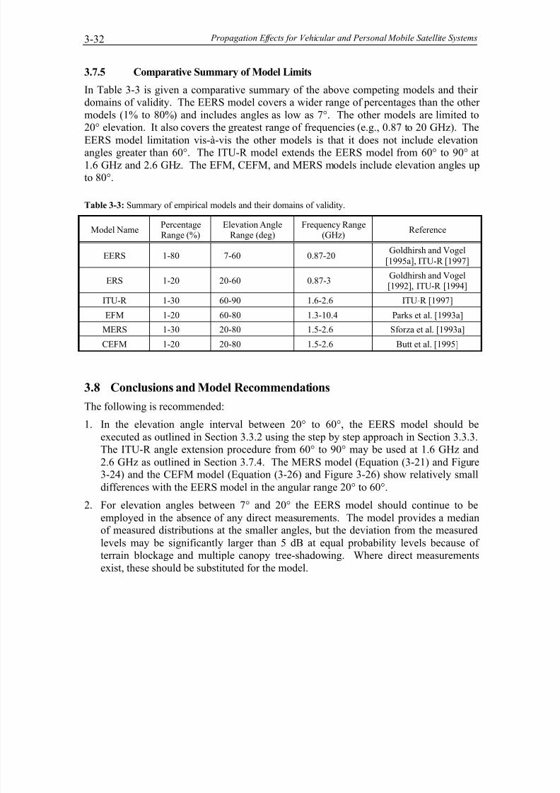
3.7.5 Comparative Summary of Model Limits_____________________________________ 3-32
3.8 Conclusions and Model Recommendations_______________________________ 3-32
3.9 References _________________________________________________________ 3-33
Table of Figures
Figure 3-1: Time-series of 1.5 GHz fade (top) and phase (bottom) over a one second period at asampling rate of 1 KHz. Measurements were taken of transmissions from MARECS-B2 at 22°
elevation along an open road near Bismarck, North Dakota............. .............. ............. ............. ...... 3-2
Figure 3-2: Time-series of 1.5 GHz fades (top) and phases (bottom) over a one second period at a
sampling rate of 1 KHz. Measurements were taken of transmissions from MARECS-B2 at 40°elevation along a highway with roadside trees in central Maryland where the satellite line-of-
sight was shadowed. ..................................................................................................................... 3-3
7/18/2019 Road side tree RF attenuation
http://slidepdf.com/reader/full/road-side-tree-rf-attenuation 4/42
3-ii
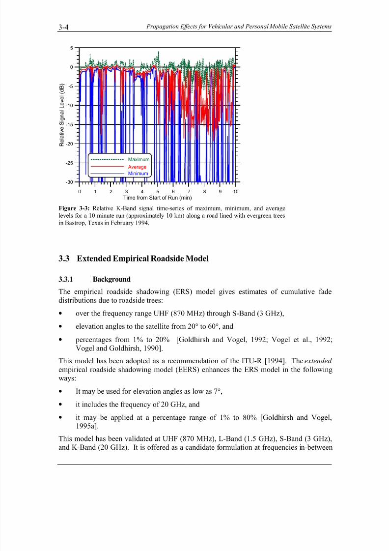
Figure 3-3: Relative K-Band signal time-series of maximum, minimum, and average levels for a
10 minute run (approximately 10 km) along a road lined with evergreen trees in Bastrop,
Texas in February 1994. ............................................................................................................... 3-4
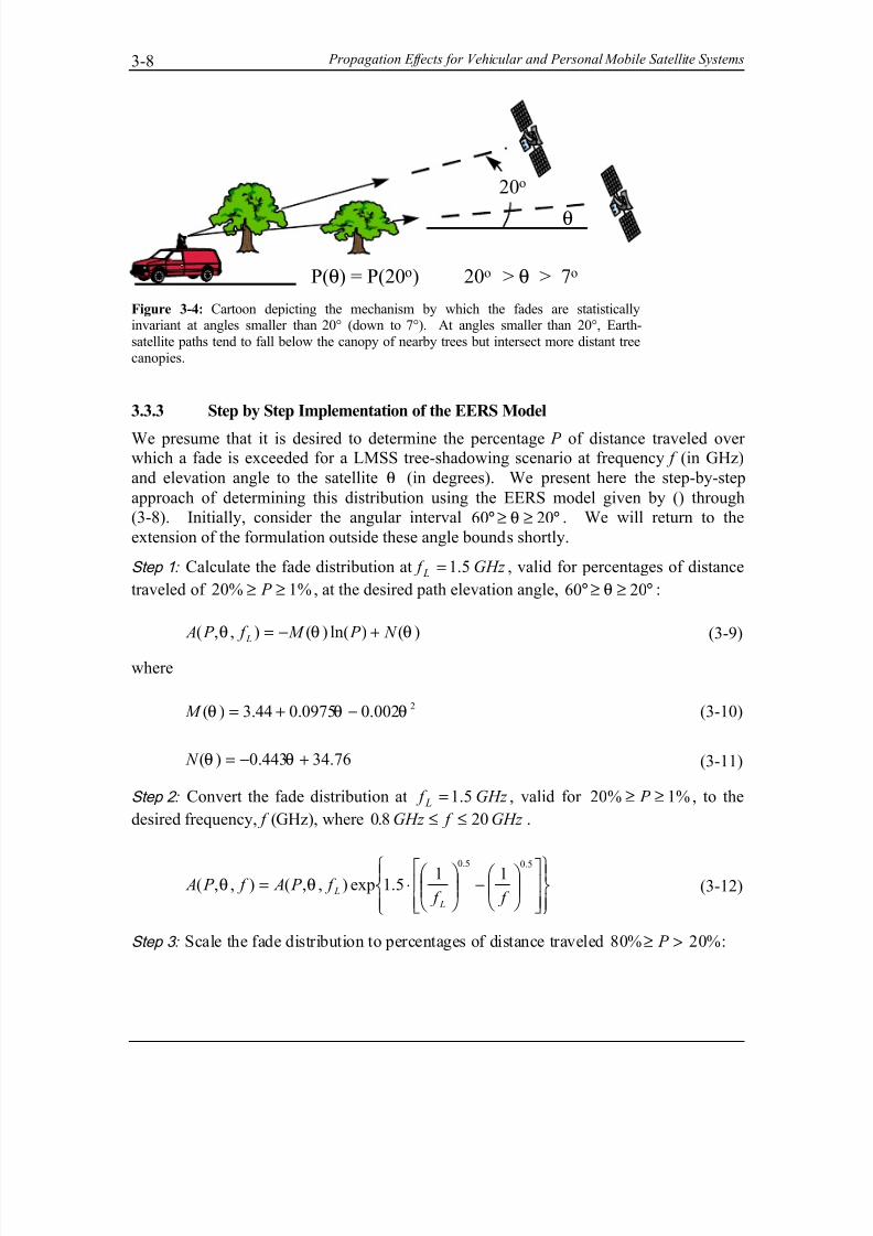
Figure 3-4: Cartoon depicting the mechanism by which the fades are statistically invariant at angles
smaller than 20° (down to 7°). At angles smaller than 20°, Earth-satellite paths tend to fall below the canopy of nearby trees but intersect more distant tree canopies. ............. .............. .......... 3-8
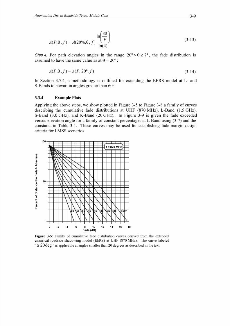
Figure 3-5: Family of cumulative fade distribution curves derived from the extended empirical
roadside shadowing model (EERS) at UHF (870 MHz). The curve labeled “ deg20≤ ” is
applicable at angles smaller than 20 degrees as described in the text... ............. ............. ............. .... 3-9
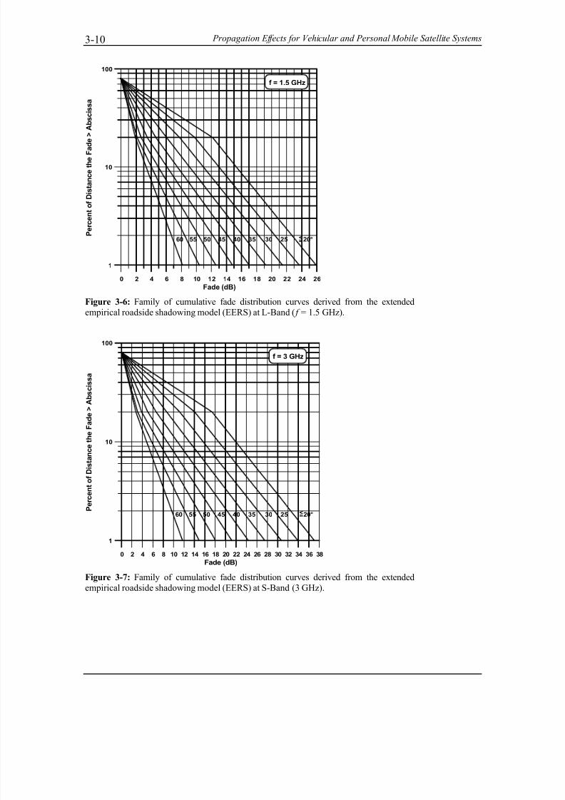
Figure 3-6: Family of cumulative fade distribution curves derived from the extended empirical
roadside shadowing model (EERS) at L-Band ( f = 1.5 GHz). ...................................................... 3-10
Figure 3-7: Family of cumulative fade distribution curves derived from the extended empirical
roadside shadowing model (EERS) at S-Band (3 GHz)....................... ............. ............. ............. .. 3-10
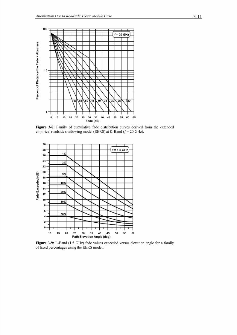
Figure 3-8: Family of cumulative fade distribution curves derived from the extended empirical
roadside shadowing model (EERS) at K-Band ( f = 20 GHz). ....................................................... 3-11
Figure 3-9: L-Band (1.5 GHz) fade values exceeded versus elevation angle for a family of fixed
percentages using the EERS model... ............. .............. ............. ............. ............. ............. ........... 3-11Figure 3-10: Comparison of EERS (solid black curve) model distribution with cumulative
distributions for eight runs in central Maryland at 1.5 GHz and elevation angle of 45°. ............ .... 3-12
Figure 3-11: Comparison of Australian fade distribution with EERS model at elevation angle of 51°
at a frequency of 1.55 GHz. ............ ............. ............. .............. ............. ............. ............. ............. 3-13
Figure 3-12: Distribution (solid) from ACTS 20 GHz measurements made in Bastrop, Texas at an
elevation angle of 54.5°. The dashed curve represents the corresponding EERS model. ............ .. 3-14
Figure 3-13: Cumulative fade distribution (solid curve) derived from L Band (1.5 GHz)
measurements in Washington State over an approximate 16 km stretch of road (elevation =
7°). The dashed curve corresponds to the EERS model distribution. ............. ............. ............. .... 3-15
Figure 3-14: K-band (20 GHz) distributions (elevation = 8°) derived from ACTS measurements in
Alaska. The solid red curve is the EERS model distribution..................... ............. .............. ........ 3-16
Figure 3-15: Plots of K-Band (20 GHz) cumulative fade distributions from measurements in central
Maryland at elevation angle of 39°............. ............. ............. .............. ............. ............. ............. .. 3-17
Figure 3-16: Measured cumulative distributions for tree shadowed environments at 18.7 GHz and
elevation angle of 32.5°, where the satellite azimuth was 90° relative to the driving direction
[Murr et al., 1995]. The dashed curved represents the EERS model. ............. ............. ............. .... 3-18
Figure 3-17: Minimum, maximum, and average fades over 1 second interval at 20 GHz for a tree-
lined run in Austin, Texas during February 6, 1994. Deciduous trees (Pecan) were devoid of
leaves. ........................................................................................................................................ 3-20
Figure 3-18: Minimum, maximum, and average fades over 1 second intervals at 20 GHz for a tree-lined run in Austin, Texas during May 2, 1994. Trees (Pecan) were in full foliage. ............. ........ 3-20
Figure 3-19: Cumulative distributions at K-Band (20 GHz) for foliage and no-foliage runs inAustin, Texas. ............................................................................................................................ 3-21
Figure 3-20: Measured and predicted levels of "foliage" versus "no-foliage" fades at 20 GHz. ............. 3-21
Figure 3-21: Independent validation of "no-foliage" versus "foliage" prediction formulation (3-15)employing static measurements in Austin, Texas at 20 GHz. Solid curves represent
measurements made during different seasons and dashed curves are the predicted levels.............. 3-22
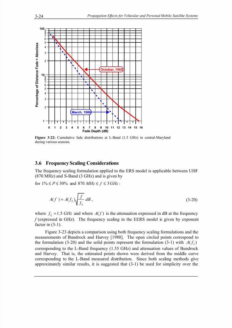
Figure 3-22: Cumulative fade distributions at L-Band (1.5 GHz) in central-Maryland during variousseasons....................................................................................................................................... 3-24
7/18/2019 Road side tree RF attenuation
http://slidepdf.com/reader/full/road-side-tree-rf-attenuation 5/42
3-iii
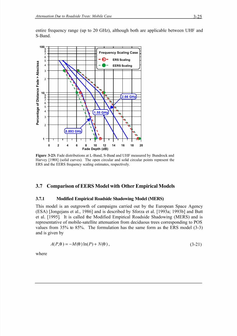
Figure 3-23: Fade distributions at L-Band, S-Band and UHF measured by Bundrock and Harvey
[1988] (solid curves). The open circular and solid circular points represent the ERS and the
EERS frequency scaling estimates, respectively. ............ ............. ............. ............. .............. ........ 3-25
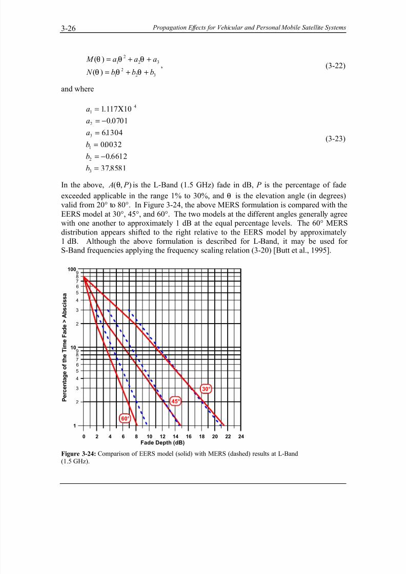
Figure 3-24: Comparison of EERS model (solid) with MERS (dashed) results at L-Band (1.5 GHz). ... 3-26
Figure 3-25: Comparison of various models at 60° elevation with EERS (solid) at 1.5 GHz. ............ .... 3-28
Figure 3-26: Comparison of EERS model (solid) with CEFM model (dashed) results at L-Band (1.5GHz). ......................................................................................................................................... 3-29
Figure 3-27: EFM and MERS model values at 70° and 80° elevations at L-Band (1.5 GHz)......... ........ 3-29
Figure 3-28: Cumulative distributions at 80° for frequencies of 1.6 and 2.6 GHz. ............. ............. ...... 3-31
Figure 3-29: Fade versus elevation angle at L-Band (1.5 GHz) with ITU-R extension to 90°........ ........ 3-31
Table of Tables
Table 3-1: Listing of parameter values of α β γ ( ), ( ), ( ) P P P in Equation (3-7). .................................3-7Table 3-2: Fades exceeded at elevations of 60° and 80°. ............. ............. .............. ............. ............. .... 3-30
Table 3-3: Summary of empirical models and their domains of validity. ............. .............. ............. ...... 3-32

7/18/2019 Road side tree RF attenuation
http://slidepdf.com/reader/full/road-side-tree-rf-attenuation 6/42
7/18/2019 Road side tree RF attenuation
http://slidepdf.com/reader/full/road-side-tree-rf-attenuation 7/42
Chapter 3
Attenuation Due to Roadside Trees: Mobile
Case
3.1 Background
In this chapter we examine measurements and empirical models associated with land-mobile satellite signal attenuation for scenarios in which a vehicle is driven along tree-
lined roads, where signal degradation is predominantly due to absorption and scatter fromtree canopies. Various models are compared with one another and with distributions
derived directly from measurements. In particular, we examine the Empirical RoadsideShadowing Model (ERS) [ITU-R, 1994, Goldhirsh and Vogel, 1992; Vogel et al., 1992],
Extended Empirical Roadside Shadowing Model (EERS) [Goldhirsh and Vogel;
1995a, 1995b], Empirical Fading Model (EFM) [Parks et al., 1993a], the CombinedEmpirical Fading Model (CEFM) [Parks et al., 1993a], and the Merged EmpiricalRoadside Shadowing Model (MERS) [Sforza et al.; 1993a; 1993b].
3.2 Time-Series Fade Measurements
In the analysis of times-series roadside fades for Land-Mobile-Satellite Service (LMSS)scenarios, the attenuation levels are represented by the dB ratio of the non-shadowed
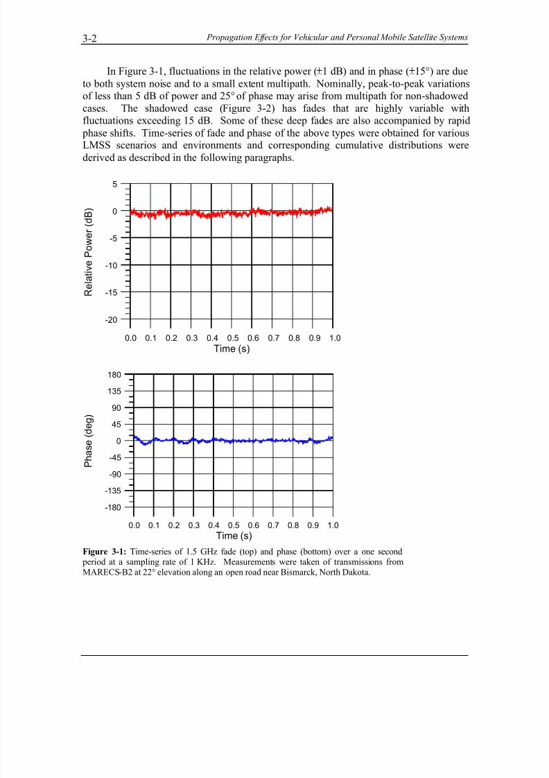
power received under conditions of negligible multipath relative to the shadowed levels.Figure 3-1 and Figure 3-2 are examples of relative power measurements depicting
nominal characteristics of fading and phase variations for non-shadowed and shadowedline-of-sight cases, respectively. These measurements were performed by Vogel and
Goldhirsh [1995] in Bismarck, North Dakota and in central-Maryland where L-Bandtransmissions (1.5 GHz) emanating from the MARECS B-2 satellite were received at
elevation angles of 22° (Figure 3-1) and 40° (Figure 3-2). The fluctuations due to
receiver noise were within 1 dB (RMS). The non-shadowed environment (Figure 3-1)
may be characterized as an open rural road and the shadowed case (Figure 3-2) a tree-lined highway where the line-of-site path was obstructed by the roadside trees.
7/18/2019 Road side tree RF attenuation
http://slidepdf.com/reader/full/road-side-tree-rf-attenuation 8/42
Propagation Effects for Vehicular and Personal Mobile Satellite Systems3-2
In Figure 3-1, fluctuations in the relative power (±1 dB) and in phase (±15°) are due
to both system noise and to a small extent multipath. Nominally, peak-to-peak variationsof less than 5 dB of power and 25°
of phase may arise from multipath for non-shadowed
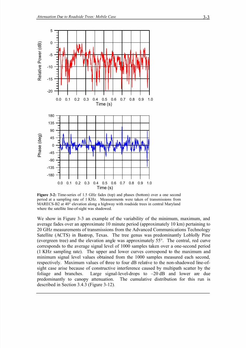
cases. The shadowed case (Figure 3-2) has fades that are highly variable withfluctuations exceeding 15 dB. Some of these deep fades are also accompanied by rapid
phase shifts. Time-series of fade and phase of the above types were obtained for variousLMSS scenarios and environments and corresponding cumulative distributions were
derived as described in the following paragraphs.
0.0 0.1 0.2 0.3 0.4 0.5 0.6 0.7 0.8 0.9 1.0
Time (s)
-20
-15
-10
-5
0
5
R e l a t i
v e P o w e r ( d B )
0.0 0.1 0.2 0.3 0.4 0.5 0.6 0.7 0.8 0.9 1.0
Time (s)
-180
-135
-90
-45
0
45
90
135
180
P h a s e ( d e g )
Figure 3-1: Time-series of 1.5 GHz fade (top) and phase (bottom) over a one second
period at a sampling rate of 1 KHz. Measurements were taken of transmissions from
MARECS-B2 at 22° elevation along an open road near Bismarck, North Dakota.
7/18/2019 Road side tree RF attenuation
http://slidepdf.com/reader/full/road-side-tree-rf-attenuation 9/42
Attenuation Due to Roadside Trees: Mobile Case 3-3
0.0 0.1 0.2 0.3 0.4 0.5 0.6 0.7 0.8 0.9 1.0
Time (s)
-20
-15
-10
-5
0
5
R e l a t i v e P o w e r ( d B )
0.0 0.1 0.2 0.3 0.4 0.5 0.6 0.7 0.8 0.9 1.0Time (s)
-180
-135
-90
-45
0
45
90
135
180
P h a s e ( d e g )
Figure 3-2: Time-series of 1.5 GHz fades (top) and phases (bottom) over a one second
period at a sampling rate of 1 KHz. Measurements were taken of transmissions from
MARECS-B2 at 40° elevation along a highway with roadside trees in central Maryland
where the satellite line-of-sight was shadowed.
We show in Figure 3-3 an example of the variability of the minimum, maximum, andaverage fades over an approximate 10 minute period (approximately 10 km) pertaining to
20 GHz measurements of transmissions from the Advanced Communications TechnologySatellite (ACTS) in Bastrop, Texas. The tree genus was predominantly Loblolly Pine(evergreen tree) and the elevation angle was approximately 55°. The central, red curve
corresponds to the average signal level of 1000 samples taken over a one-second period(1 KHz sampling rate). The upper and lower curves correspond to the maximum and
minimum signal level values obtained from the 1000 samples measured each second,respectively. Maximum values of three to four dB relative to the non-shadowed line-of-
sight case arise because of constructive interference caused by multipath scatter by thefoliage and branches. Large signal-level-drops to –20 dB and lower are due
predominantly to canopy attenuation. The cumulative distribution for this run isdescribed in Section 3.4.3 (Figure 3-12).
7/18/2019 Road side tree RF attenuation
http://slidepdf.com/reader/full/road-side-tree-rf-attenuation 10/42
Propagation Effects for Vehicular and Personal Mobile Satellite Systems3-4
0 1 2 3 4 5 6 7 8 9 10Time from Start of Run (min)
-30
-25
-20
-15
-10
-5
0
5
R e l a t i v e S i g n a l L e v e l
( d B )
Maximum
Average
Minimum
Figure 3-3: Relative K-Band signal time-series of maximum, minimum, and average
levels for a 10 minute run (approximately 10 km) along a road lined with evergreen trees
in Bastrop, Texas in February 1994.
3.3 Extended Empirical Roadside Model
3.3.1 Background
The empirical roadside shadowing (ERS) model gives estimates of cumulative fadedistributions due to roadside trees:
• over the frequency range UHF (870 MHz) through S-Band (3 GHz),
• elevation angles to the satellite from 20° to 60°, and
• percentages from 1% to 20% [Goldhirsh and Vogel, 1992; Vogel et al., 1992;Vogel and Goldhirsh, 1990].
This model has been adopted as a recommendation of the ITU-R [1994]. The extended empirical roadside shadowing model (EERS) enhances the ERS model in the followingways:
• It may be used for elevation angles as low as 7°,
• it includes the frequency of 20 GHz, and
• it may be applied at a percentage range of 1% to 80% [Goldhirsh and Vogel,1995a].
This model has been validated at UHF (870 MHz), L-Band (1.5 GHz), S-Band (3 GHz),and K-Band (20 GHz). It is offered as a candidate formulation at frequencies in-between
7/18/2019 Road side tree RF attenuation
http://slidepdf.com/reader/full/road-side-tree-rf-attenuation 11/42
Attenuation Due to Roadside Trees: Mobile Case 3-5
3 GHz and 20 GHz and at higher frequencies (e.g., 30 GHz) until data becomes available
for validation. This revised model was adopted by the ITU-R in 1997 [ITU-R, 1997].
The ERS model was derived from the median of cumulative UHF and L-Band fade
distributions systematically obtained from helicopter-mobile and satellite-mobilemeasurements in central Maryland. The measurements were made over approximately
600 km of driving distance comprising path elevation angles of 21°, 30°, 45° and 60°.The 21° case was executed employing the geostationary satellite MARECS-B2 [Vogel
and Goldhirsh, 1990], whereas the measurements for the other angles were obtainedemploying a helicopter as the transmitter platform [Goldhirsh and Vogel, 1987; 1989].
The configuration corresponds to a shadowing condition in which the helicopter flew parallel to the moving vehicle and the propagation path was approximately normal to the
line of roadside trees (e.g., azimuth of the satellite relative to the vehicle direction was90°). Tree heights ranged from approximately 5 to 30 m. The satellite path directions
were such that these were also predominantly along 90° shadowing orientation, althoughsome of the roads sampled had a number of bends in them and deviations from this aspect
did arise. The measurements were performed on two-lane highways (one lane in each
direction), and a four-lane highway (two lanes in each direction), where the roadside treeswere primarily of the deciduous variety. In order to assess the extent by which trees populate the side of the road, a quantity called percentage of optical shadowing (POS)
was defined. This represents the percentage of optical shadowing caused by roadsidetrees at a path angle of 45° for right side of the road driving, where the path is to the right
of the driver and the vehicle is in the right lane. The POS values for the roads drivenwere predominantly between 55% and 75% implying tree populations of at least these
amounts.
In deriving the EERS model, use was made of the original previously developed
body of data at UHF and L-Band in central Maryland as well as more recent developeddatabases. These correspond to mobile L-Band measurements of transmissions from
MARECS B-2 in the western United States [Vogel and Goldhirsh, 1995], static K-Band(20 GHz) measurements in Austin, Texas [Vogel and Goldhirsh, 1993a; 1993b], and
mobile K-Band measurements employing transmissions from ACTS [Goldhirsh andVogel, 1995a; 1995b]. These latter measurements were performed during the first six
months of 1994 during which a series of four 20 GHz mobile-ACTS campaigns wereexecuted. The campaigns were performed in central Maryland (March, elevation = 39°),
Austin, Texas (February and May, elevation = 55°) and Fairbanks, Alaska and environs(June, elevation = 8°). The mobile measurements in Austin, Texas during February and
May enabled a determination of 20 GHz fading probability distributions for no-foliageand foliage conditions, respectively.
3.3.2 EERS Formulation
In the following paragraphs is given an overview of the EERS formulation followed by
examples of its validation.
For 20% 1%≥ ≥ P and 20 60°≤ ≤ °θ
7/18/2019 Road side tree RF attenuation
http://slidepdf.com/reader/full/road-side-tree-rf-attenuation 12/42
Propagation Effects for Vehicular and Personal Mobile Satellite Systems3-6
−
⋅=
5.05.0
115.1exp),,(),,(
f f f P A f P A
L
Lθθ (3-1)
and for 80% 20%≥ > P and 20 60°≤ ≤ °θ
)4ln(
80ln
),%,20(),,(
= P f A f P A θθ
(3-2)
where A P f ( , , )θ is the attenuation (in dB) at the frequency f (in GHz) exceeded at P (in
%) which represents the percentage of the driving distance for an Earth-satellite pathangle θ (in degrees), and A P f L( , , )θ is the corresponding attenuation (in dB) at f L =
1.5 GHz. The attenuation is defined relative to non-shadowed and negligible multipathconditions.
The L-Band attenuation at f L = 1.5 GHz (i.e., A P f L( , , )θ ) for 20% 1%≥ ≥ P and
20 60°≤ ≤ °θ is given by
)()ln()(),,( θθθ N P M f P A L +−= (3-3)
where
2)( θθθ cba M ++= (3-4)
ed N += θθ )( (3-5)
and where
76.34
443.0
002.0
0975.0
44.3
=−=−=
==
e
d
c
b
a
(3-6)
In Equation (3-3), P is in %, θ is in degrees, f is in GHz, and A P f L( , , )θ is in dB.
Substituting (3-4) through (3-6) into (3-3), A P f L( , , )θ may alternately be expressed by
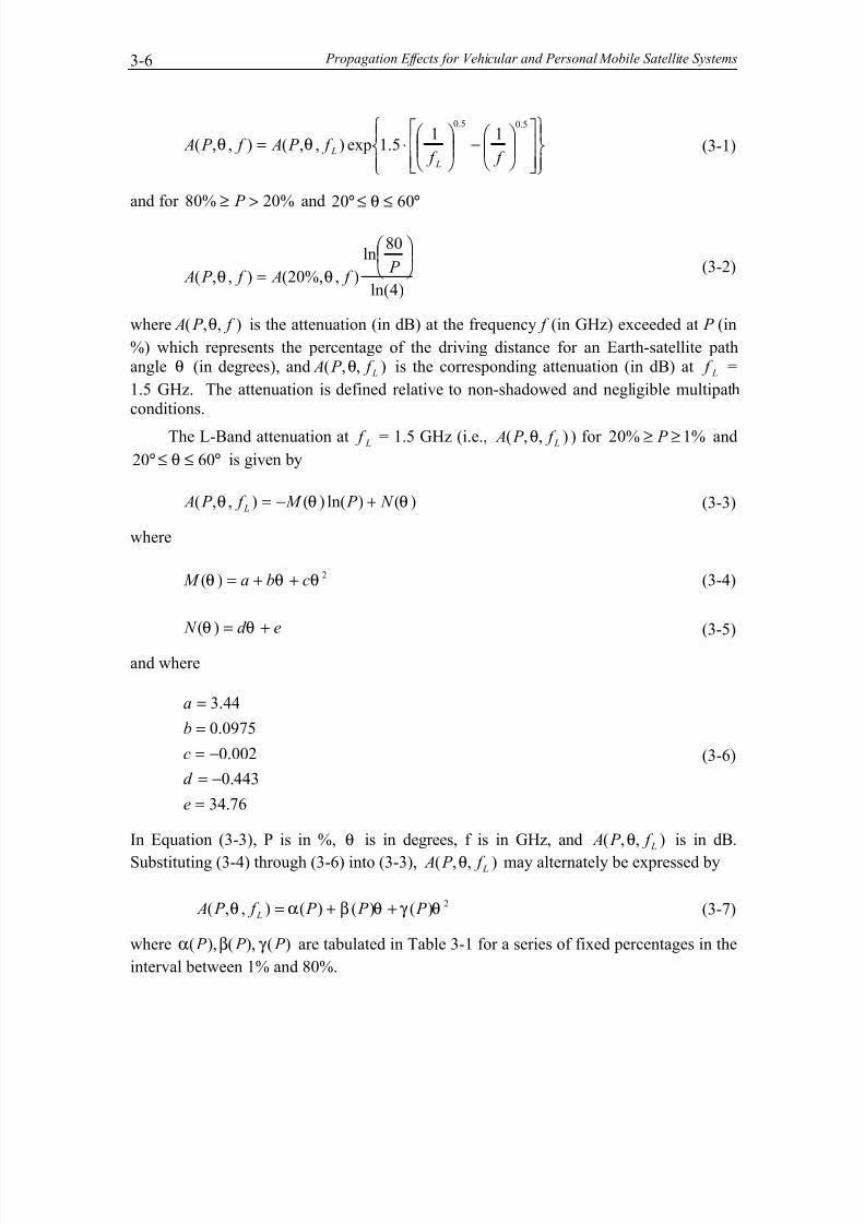
2)()()(),,( θγ θβαθ P P P f P A L ++= (3-7)
where α β γ ( ), ( ), ( ) P P P are tabulated in Table 3-1 for a series of fixed percentages in the
interval between 1% and 80%.
7/18/2019 Road side tree RF attenuation
http://slidepdf.com/reader/full/road-side-tree-rf-attenuation 13/42
Attenuation Due to Roadside Trees: Mobile Case 3-7
Table 3-1: Listing of parameter values of α β γ ( ), ( ), ( ) P P P in Equation (3-7).
Percentage, P α( ) P β( ) P γ ( ) P
1 34.7600 -0.4430 0.0
2 32.3756 -0.5106 1.3863X10⁻³
5 29.2235 -0.5999 3.2189X10⁻³
10 26.8391 -0.6675 4.6052X10⁻³
20 24.4547 -0.7351 5.9915X10⁻³
30 17.3022 -0.5201 4.2391X10⁻³
40 12.2273 -0.36754 2.9957X10⁻³
50 8.2910 -0.2492 2.0313X10⁻³
60 5.0748 -0.1525 1.2433X10⁻³
70 2.3556 -7.0805X10⁻²
5.7711X10⁻⁴
80 0.0 0.0 0.0
For the case in which 20 7° > ≥ °θ , the distribution derived using the formulations () or
(3-7) is first calculated at θ = °20 . This distribution for θ = °20 is subsequently assumed
to be invariant at the smaller elevation angles. That is,
for 80% 1%≥ ≥ P and 20 7° > ≥ °θ
),20,(),,( f P A f P A °=θ . (3-8)
Equation (3-8) implies that the probability distributions at elevation angles smaller than
20° are the same as those at 20°. Extending the model to elevation angles smaller than20° is a complex task for the following reasons: (1) The EERS model tacitly assumes
that the canopies of single trees shadow the Earth-satellite path. At lower angles, theremay be a greater likelihood that the path cuts the canopies of multiple trees or multiple
tree trunks. (2) At smaller angles, there may also be a greater likelihood that the terrainitself blocks the Earth-satellite path creating high attenuation. (3) Ground multipath may
also influence the distribution considerably. Based upon empirical experience for caseswhere the above caveats did not arise, it has been found that with good approximation the
EERS model at 20° elevation is representative of results at 7° or 8°. The rationale for thisassumption is characterized in Figure 3-4. At 20° elevation, the Earth-satellite path is
already passing through the lower part of the tree canopies. Reducing the path elevationangle is likely to result in attenuation caused by tree trunks that may tend to mitigate the
signal degradation. On the other hand, attenuation effects may increase because of fadingfrom those tree canopies that are further offset from the road (as was the case in Alaska).
The combination of these two effects generally results in the median fade statistics to berelatively invariant to angles below 20°, although larger deviations about the median are
expected because of the breakdown of the aforementioned underlying assumptions.
7/18/2019 Road side tree RF attenuation
http://slidepdf.com/reader/full/road-side-tree-rf-attenuation 14/42
Propagation Effects for Vehicular and Personal Mobile Satellite Systems3-8
P(θ) = P(20ο) 20o > θ > 7o
θ
20o
Figure 3-4: Cartoon depicting the mechanism by which the fades are statisticallyinvariant at angles smaller than 20° (down to 7°). At angles smaller than 20°, Earth-
satellite paths tend to fall below the canopy of nearby trees but intersect more distant tree
canopies.
3.3.3 Step by Step Implementation of the EERS Model
We presume that it is desired to determine the percentage P of distance traveled over which a fade is exceeded for a LMSS tree-shadowing scenario at frequency f (in GHz)
and elevation angle to the satellite θ (in degrees). We present here the step-by-step
approach of determining this distribution using the EERS model given by () through
(3-8). Initially, consider the angular interval 60 20°≥ ≥ °θ . We will return to the
extension of the formulation outside these angle bounds shortly.
Step 1 : Calculate the fade distribution at GHz f L 5.1= , valid for percentages of distance
traveled of 20% 1%≥ ≥ P , at the desired path elevation angle, 60 20°≥ ≥ °θ :
)()ln()(),,( θθθ N P M f P A L +−= (3-9)
where
2002.00975.044.3)( θθθ −+= M (3-10)
76.34443.0)( +−= θθ N (3-11)
Step 2 : Convert the fade distribution at GHz f L 5.1= , valid for 20% 1%≥ ≥ P , to the
desired frequency, f (GHz), where 0 8 20. GHz f GHz ≤ ≤ .
−
⋅=
5.05.0 115.1exp),,(),,(
f f f P A f P A
L
Lθθ (3-12)
Step 3 : Scale the fade distribution to percentages of distance traveled 80% 20%≥ > P :
7/18/2019 Road side tree RF attenuation
http://slidepdf.com/reader/full/road-side-tree-rf-attenuation 15/42
Attenuation Due to Roadside Trees: Mobile Case 3-9
)4ln(
80ln
),%,20(),,(
= P f A f P A θθ
(3-13)
Step 4 : For path elevation angles in the range 20 7° > ≥ °θ , the fade distribution isassumed to have the same value as at θ = °20 :
),20,(),,( f P A f P A °=θ (3-14)
In Section 3.7.4, a methodology is outlined for extending the EERS model at L- andS-Bands to elevation angles greater than 60°.
3.3.4 Example Plots
Applying the above steps, we show plotted in Figure 3-5 to Figure 3-8 a family of curves
describing the cumulative fade distributions at UHF (870 MHz), L-Band (1.5 GHz),
S-Band (3.0 GHz), and K-Band (20 GHz). In Figure 3-9 is given the fade exceededversus elevation angle for a family of constant percentages at L Band using (3-7) and theconstants in Table 3-1. These curves may be used for establishing fade-margin design
criteria for LMSS scenarios.
0 2 4 6 8 10 12 14 16 18
Fade (dB)
1
10
100
P e r c e n t o f D i s t a n c e t h e F a d e > A b s c i s s a
2530354045505560 20°<=
f = 870 MHz
Figure 3-5: Family of cumulative fade distribution curves derived from the extended
empirical roadside shadowing model (EERS) at UHF (870 MHz). The curve labeled
“ deg20≤ ” is applicable at angles smaller than 20 degrees as described in the text.
7/18/2019 Road side tree RF attenuation
http://slidepdf.com/reader/full/road-side-tree-rf-attenuation 16/42
Propagation Effects for Vehicular and Personal Mobile Satellite Systems3-10
0 2 4 6 8 10 12 14 16 18 20 22 24 26Fade (dB)
1
10
100
P e r c e n t o f D i s t a n c e t h e F a d e
> A b s c i s s a
2530354045505560 20°<=
f = 1.5 GHz
Figure 3-6: Family of cumulative fade distribution curves derived from the extended
empirical roadside shadowing model (EERS) at L-Band ( f = 1.5 GHz).
0 2 4 6 8 10 12 14 16 18 20 22 24 26 28 30 32 34 36 38
Fade (dB)
1
10
100
P e r c e n t o f D i s t a n c e t h e F a d
e > A b s c i s s a
2530354045505560 20°<=
f = 3 GHz
Figure 3-7: Family of cumulative fade distribution curves derived from the extended
empirical roadside shadowing model (EERS) at S-Band (3 GHz).
7/18/2019 Road side tree RF attenuation
http://slidepdf.com/reader/full/road-side-tree-rf-attenuation 17/42
Attenuation Due to Roadside Trees: Mobile Case 3-11
0 5 10 15 20 25 30 35 40 45 50 55 60 65Fade (dB)
1
10
100
P e r c e n t o f D i s t a n c e t h e F a d e
> A b s c i s s a
2530354045505560 20°<=
f = 20 GHz
Figure 3-8: Family of cumulative fade distribution curves derived from the extended
empirical roadside shadowing model (EERS) at K-Band ( f = 20 GHz).
10 15 20 25 30 35 40 45 50 55 60
Path Elevation Angle (deg)
0
2
4
6
8
10
12
14
16
18
20
22
24
26
28
30
F a d e E x c e e d e d ( d
B )
1%
2%
5%
10%
20%
30%
50%
f = 1.5 GHz
Figure 3-9: L-Band (1.5 GHz) fade values exceeded versus elevation angle for a family
of fixed percentages using the EERS model.
7/18/2019 Road side tree RF attenuation
http://slidepdf.com/reader/full/road-side-tree-rf-attenuation 18/42
Propagation Effects for Vehicular and Personal Mobile Satellite Systems3-12
3.4 Validation of the Extended Empirical Roadside Shadowing Model
3.4.1 Central Maryland at L-Band
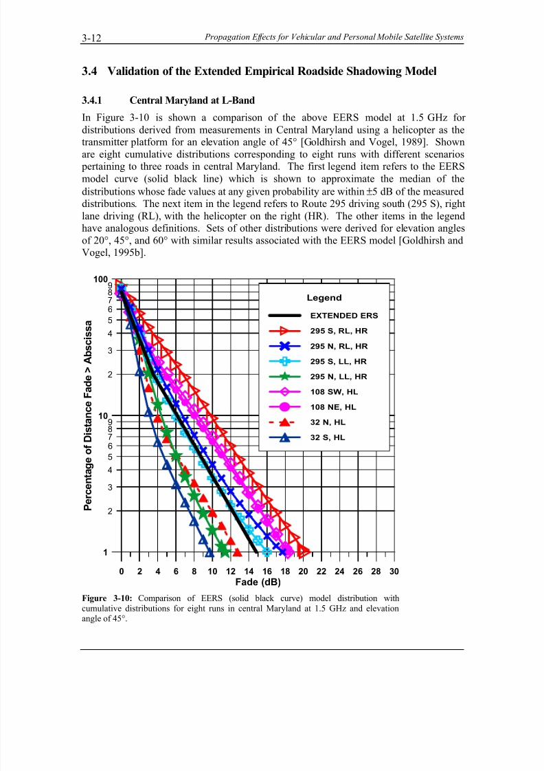
In Figure 3-10 is shown a comparison of the above EERS model at 1.5 GHz for
distributions derived from measurements in Central Maryland using a helicopter as thetransmitter platform for an elevation angle of 45° [Goldhirsh and Vogel, 1989]. Shown
are eight cumulative distributions corresponding to eight runs with different scenarios pertaining to three roads in central Maryland. The first legend item refers to the EERS
model curve (solid black line) which is shown to approximate the median of the
distributions whose fade values at any given probability are within ±5 dB of the measureddistributions. The next item in the legend refers to Route 295 driving south (295 S), right
lane driving (RL), with the helicopter on the right (HR). The other items in the legendhave analogous definitions. Sets of other distributions were derived for elevation angles
of 20°, 45°, and 60° with similar results associated with the EERS model [Goldhirsh andVogel, 1995b].
0 2 4 6 8 10 12 14 16 18 20 22 24 26 28 30
Fade (dB)
2
3
4
5
6789
2
3
4
5
6789
1
10
100
P e r c e n t a g e o f D i s t a n c e
F a d e > A b s c i s s a
Legend
EXTENDED ERS
295 S, RL, HR
295 N, RL, HR
295 S, LL, HR
295 N, LL, HR
108 SW, HL
108 NE, HL
32 N, HL
32 S, HL
Figure 3-10: Comparison of EERS (solid black curve) model distribution with
cumulative distributions for eight runs in central Maryland at 1.5 GHz and elevationangle of 45°.
7/18/2019 Road side tree RF attenuation
http://slidepdf.com/reader/full/road-side-tree-rf-attenuation 19/42
Attenuation Due to Roadside Trees: Mobile Case 3-13
3.4.2 Australian Fade Distributions at L-Band
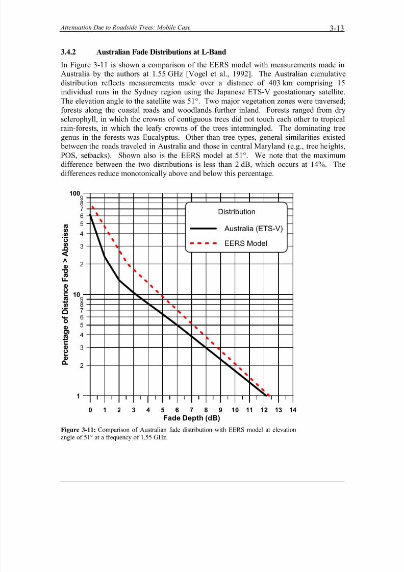
In Figure 3-11 is shown a comparison of the EERS model with measurements made inAustralia by the authors at 1.55 GHz [Vogel et al., 1992]. The Australian cumulative
distribution reflects measurements made over a distance of 403 km comprising 15individual runs in the Sydney region using the Japanese ETS-V geostationary satellite.
The elevation angle to the satellite was 51°. Two major vegetation zones were traversed;forests along the coastal roads and woodlands further inland. Forests ranged from dry
sclerophyll, in which the crowns of contiguous trees did not touch each other to tropicalrain-forests, in which the leafy crowns of the trees intermingled. The dominating tree
genus in the forests was Eucalyptus. Other than tree types, general similarities existed between the roads traveled in Australia and those in central Maryland (e.g., tree heights,
POS, setbacks). Shown also is the EERS model at 51°. We note that the maximumdifference between the two distributions is less than 2 dB, which occurs at 14%. The
differences reduce monotonically above and below this percentage.
0 1 2 3 4 5 6 7 8 9 10 11 12 13 14
Fade Depth (dB)
2
3
4
5
6789
2
3
4
5
6789
1
10
100
P e r c e n t a g e o f D i s t a n c e F a d e > A b s c i s s a
Distribution
Australia (ETS-V)
EERS Model
Figure 3-11: Comparison of Australian fade distribution with EERS model at elevation
angle of 51° at a frequency of 1.55 GHz.
7/18/2019 Road side tree RF attenuation
http://slidepdf.com/reader/full/road-side-tree-rf-attenuation 20/42
Propagation Effects for Vehicular and Personal Mobile Satellite Systems3-14
3.4.3 Austin, Texas at K-Band
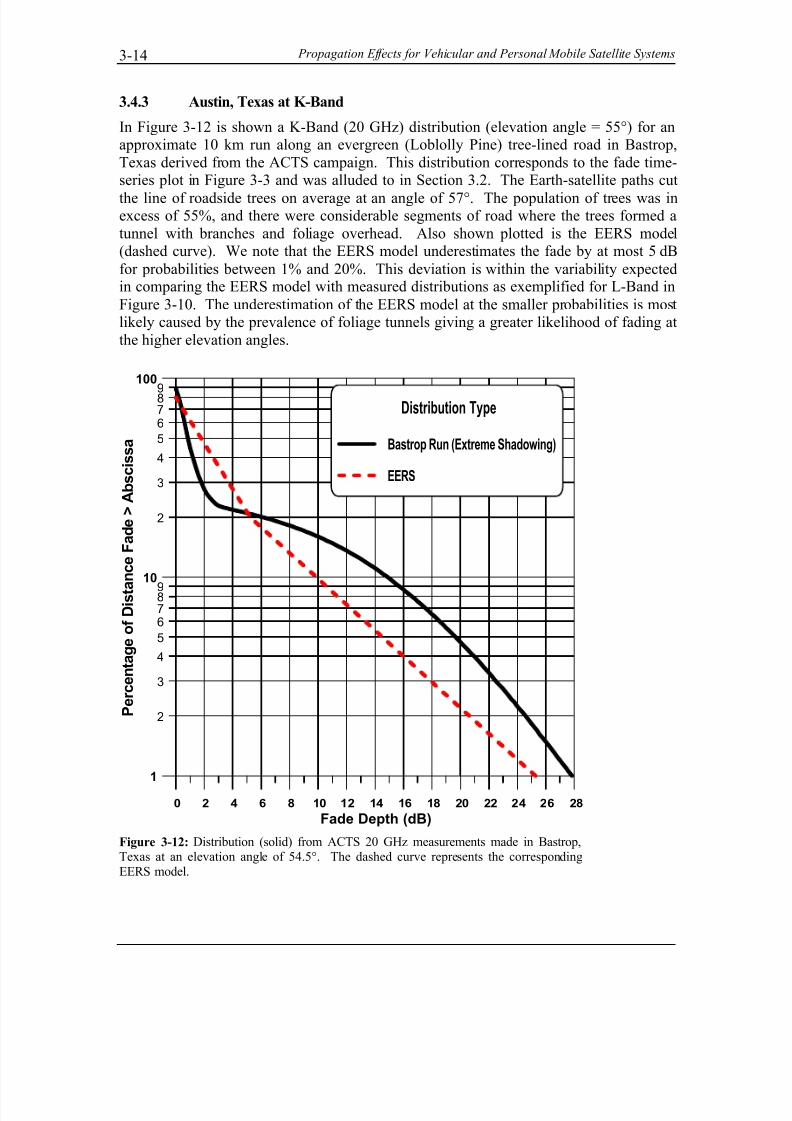
In Figure 3-12 is shown a K-Band (20 GHz) distribution (elevation angle = 55°) for anapproximate 10 km run along an evergreen (Loblolly Pine) tree-lined road in Bastrop,
Texas derived from the ACTS campaign. This distribution corresponds to the fade time-series plot in Figure 3-3 and was alluded to in Section 3.2. The Earth-satellite paths cut
the line of roadside trees on average at an angle of 57°. The population of trees was inexcess of 55%, and there were considerable segments of road where the trees formed a
tunnel with branches and foliage overhead. Also shown plotted is the EERS model(dashed curve). We note that the EERS model underestimates the fade by at most 5 dB
for probabilities between 1% and 20%. This deviation is within the variability expectedin comparing the EERS model with measured distributions as exemplified for L-Band in
Figure 3-10. The underestimation of the EERS model at the smaller probabilities is mostlikely caused by the prevalence of foliage tunnels giving a greater likelihood of fading at
the higher elevation angles.
0 2 4 6 8 10 12 14 16 18 20 22 24 26 28
Fade Depth (dB)
2
3
4
5
6789
2
3
4
5
6789
1
10
100
P e r c e n t a g e o f D i s t a
n c e F a d e > A b s c i s s a
Distribution Type
Bastrop Run (Extreme Shadowing)
EERS
Figure 3-12: Distribution (solid) from ACTS 20 GHz measurements made in Bastrop,
Texas at an elevation angle of 54.5°. The dashed curve represents the corresponding
EERS model.
7/18/2019 Road side tree RF attenuation
http://slidepdf.com/reader/full/road-side-tree-rf-attenuation 21/42
Attenuation Due to Roadside Trees: Mobile Case 3-15
3.4.4 Low Angle Measurements in Washington State at L-Band
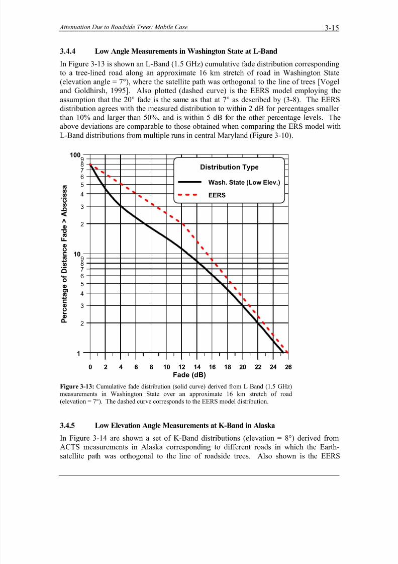
In Figure 3-13 is shown an L-Band (1.5 GHz) cumulative fade distribution correspondingto a tree-lined road along an approximate 16 km stretch of road in Washington State
(elevation angle = 7°), where the satellite path was orthogonal to the line of trees [Vogeland Goldhirsh, 1995]. Also plotted (dashed curve) is the EERS model employing the
assumption that the 20° fade is the same as that at 7° as described by (3-8). The EERSdistribution agrees with the measured distribution to within 2 dB for percentages smaller
than 10% and larger than 50%, and is within 5 dB for the other percentage levels. Theabove deviations are comparable to those obtained when comparing the ERS model with
L-Band distributions from multiple runs in central Maryland (Figure 3-10).
0 2 4 6 8 10 12 14 16 18 20 22 24 26
Fade (dB)
2
34
5
6789
2
34
5
6789
1
10
100
P e r c e n t a
g e o f D i s t a n c e F a d e > A b s c i s s a
Distribution Type
Wash. State (Low Elev.)
EERS
Figure 3-13: Cumulative fade distribution (solid curve) derived from L Band (1.5 GHz)
measurements in Washington State over an approximate 16 km stretch of road(elevation = 7°). The dashed curve corresponds to the EERS model distribution.
3.4.5 Low Elevation Angle Measurements at K-Band in Alaska
In Figure 3-14 are shown a set of K-Band distributions (elevation = 8°) derived fromACTS measurements in Alaska corresponding to different roads in which the Earth-
satellite path was orthogonal to the line of roadside trees. Also shown is the EERS
7/18/2019 Road side tree RF attenuation
http://slidepdf.com/reader/full/road-side-tree-rf-attenuation 22/42
Propagation Effects for Vehicular and Personal Mobile Satellite Systems3-16
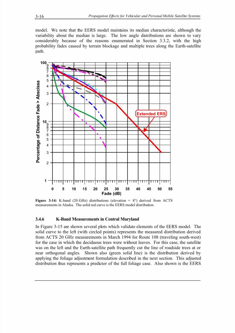
model. We note that the EERS model maintains its median characteristic, although the
variability about the median is large. The low angle distributions are shown to varyconsiderably because of the reasons enumerated in Section 3.3.2, with the high
probability fades caused by terrain blockage and multiple trees along the Earth-satellite path.
0 5 10 15 20 25 30 35 40 45 50 55
Fade (dB)
2
3
4
5
6789
2
3
4
5
6789
1
10
100
P e r c e n t a g e o f D i s t a n c e
F a d e > A b s c i s s a
Extended ERS
Figure 3-14: K-band (20 GHz) distributions (elevation = 8°) derived from ACTS
measurements in Alaska. The solid red curve is the EERS model distribution.
3.4.6 K-Band Measurements in Central Maryland
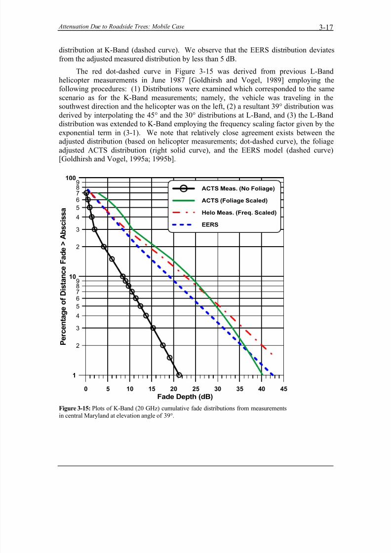
In Figure 3-15 are shown several plots which validate elements of the EERS model. The
solid curve to the left (with circled points) represents the measured distribution derivedfrom ACTS 20 GHz measurements in March 1994 for Route 108 (traveling south-west)for the case in which the deciduous trees were without leaves. For this case, the satellite
was on the left and the Earth-satellite path frequently cut the line of roadside trees at or near orthogonal angles. Shown also (green solid line) is the distribution derived by
applying the foliage adjustment formulation described in the next section. This adjusteddistribution thus represents a predictor of the full foliage case. Also shown is the EERS
7/18/2019 Road side tree RF attenuation
http://slidepdf.com/reader/full/road-side-tree-rf-attenuation 23/42
Attenuation Due to Roadside Trees: Mobile Case 3-17
distribution at K-Band (dashed curve). We observe that the EERS distribution deviates
from the adjusted measured distribution by less than 5 dB.
The red dot-dashed curve in Figure 3-15 was derived from previous L-Band
helicopter measurements in June 1987 [Goldhirsh and Vogel, 1989] employing thefollowing procedures: (1) Distributions were examined which corresponded to the same
scenario as for the K-Band measurements; namely, the vehicle was traveling in thesouthwest direction and the helicopter was on the left, (2) a resultant 39° distribution was
derived by interpolating the 45° and the 30° distributions at L-Band, and (3) the L-Banddistribution was extended to K-Band employing the frequency scaling factor given by the
exponential term in (3-1). We note that relatively close agreement exists between theadjusted distribution (based on helicopter measurements; dot-dashed curve), the foliage
adjusted ACTS distribution (right solid curve), and the EERS model (dashed curve)[Goldhirsh and Vogel, 1995a; 1995b].
0 5 10 15 20 25 30 35 40 45Fade Depth (dB)
2
3
4
5
6789
2
3
4
5
67
89
1
10
100
P e r c e n t a g e o f D i
s t a n c e F a d e > A b s c i s s a
ACTS Meas. (No Foliage)
ACTS (Foliage Scaled)
Helo Meas. (Freq. Scaled)
EERS
Figure 3-15: Plots of K-Band (20 GHz) cumulative fade distributions from measurements
in central Maryland at elevation angle of 39°.
7/18/2019 Road side tree RF attenuation
http://slidepdf.com/reader/full/road-side-tree-rf-attenuation 24/42
Propagation Effects for Vehicular and Personal Mobile Satellite Systems3-18
3.4.7 Comparison with ESA K-Band Measurements
We compare here EERS model distributions at 18.7 GHz with measured distributions byMurr et al. [1995] obtained in a series of campaigns supported by the European Space
Agency (ESA). The campaigns used a radiating source on board the geostationarysatellite Italsat F1 [Paraboni and Giannone, 1991] and a mobile van with a tracking
antenna [Joanneum Research, 1995]. The elevation angles were between 30° and 35° anda number of runs in four European countries were executed for different driving
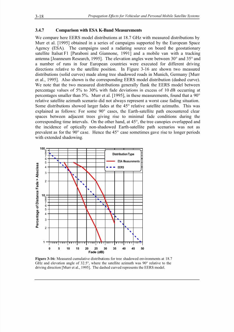
directions relative to the satellite position. In Figure 3-16 are shown two measureddistributions (solid curves) made along tree shadowed roads in Munich, Germany [Murr
et al., 1995]. Also shown is the corresponding EERS model distribution (dashed curve).We note that the two measured distributions generally flank the EERS model between
percentage values of 5% to 30% with fade deviations in excess of 10 dB occurring at percentages smaller than 5%. Murr et al. [1995], in these measurements, found that a 90°
relative satellite azimuth scenario did not always represent a worst case fading situation.Some distributions showed larger fades at the 45° relative satellite azimuths. This was
explained as follows: For some 90° cases, the Earth-satellite path encountered clear
spaces between adjacent trees giving rise to minimal fade conditions during thecorresponding time intervals. On the other hand, at 45°, the tree canopies overlapped andthe incidence of optically non-shadowed Earth-satellite path scenarios was not as
prevalent as for the 90° case. Hence the 45° case sometimes gave rise to longer periodswith extended shadowing.
0 5 10 15 20 25 30 35 40 45 50
Fade (dB)
2
3
4
5
6789
2
3
4
5
6789
1
10
100
P e r c e n t a g e o f D i s t a n c e F a d e > A b
s c i s s a
Distribution Type
ESA Measurements
EERS
Figure 3-16: Measured cumulative distributions for tree shadowed environments at 18.7
GHz and elevation angle of 32.5°, where the satellite azimuth was 90° relative to the
driving direction [Murr et al., 1995]. The dashed curved represents the EERS model.
7/18/2019 Road side tree RF attenuation
http://slidepdf.com/reader/full/road-side-tree-rf-attenuation 25/42
Attenuation Due to Roadside Trees: Mobile Case 3-19
3.5 Attenuation Effects of Foliage
3.5.1 K-Band Effects
Measurements made in Austin, Texas during February and May when the trees were
without and with leaves, respectively, enabled a “foliage’’ adjustment model to bedeveloped. The formulation relates equal probability attenuation (dB) corresponding to
“foliage” and “no-foliage” cases at K-Band and is given by
C Foliage NobAa Foliage A )()( += (3-15)
a
b
c
===
0351
68253
05776
.
.
.
, (3-16)
and where
dB Foliage No A 15)(1 ≤≤ and (3-17)
dB Foliage A 32)(8 ≤≤ . (3-18)
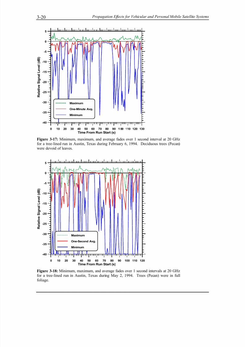
This formulation was derived from “no-foliage” and “foliage” mobile measurementsmade during February and May of 1994, respectively, in Austin, Texas during the ACTS
campaigns. The time-series signal level characteristics for these two cases are shown inFigure 3-17 and Figure 3-18, where the measurements were made along a one kilometer
segment of a street heavily populated with Pecan trees. Shown are the minimum,maximum, and average signal levels over one second periods for a sampling rate of
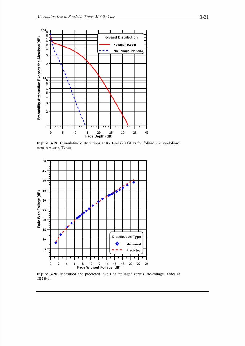
1 KHz. The corresponding cumulative fade distributions are shown in Figure 3-19 wherethe dashed and solid curves correspond to the “no-foliage” and “foliage” cases. Thedirection of travel for these runs was approximately orthogonal to the satellite pointing
direction. The optical blockage to the satellite during the full foliage period wasestimated to be well in excess of 55%. Performing a least square fit associated with equal
probability levels of the attenuation for the two curves in Figure 3-19, the formulation(3-15) was derived. A comparison of the measured and predicted levels describing the
foliage versus no foliage fades is given in Figure 3-20. The predicted curve (dashed) isshown to agree to within a fraction of a dB up to fades (with foliage) of approximately
38 dB.
7/18/2019 Road side tree RF attenuation
http://slidepdf.com/reader/full/road-side-tree-rf-attenuation 26/42
Propagation Effects for Vehicular and Personal Mobile Satellite Systems3-20
0 10 20 30 40 50 60 70 80 90 1 00 110 120 130
Time From Run Start (s)
-40
-35
-30
-25
-20
-15
-10
-5
0
5
R e l a t i v e S i g n a l L e v e l ( d B )
Maximum
One-Minute Avg.
Minimum
Figure 3-17: Minimum, maximum, and average fades over 1 second interval at 20 GHzfor a tree-lined run in Austin, Texas during February 6, 1994. Deciduous trees (Pecan)were devoid of leaves.
0 10 20 30 40 50 60 70 80 90 100 110 120
Time From Run Start (s)
-40
-35
-30
-25
-20
-15
-10
-5
0
5
R e l a t i v e S i g n a l L e v e l ( d B )
Maximum
One-Second Avg.
Minimum
Figure 3-18: Minimum, maximum, and average fades over 1 second intervals at 20 GHz
for a tree-lined run in Austin, Texas during May 2, 1994. Trees (Pecan) were in full
foliage.
7/18/2019 Road side tree RF attenuation
http://slidepdf.com/reader/full/road-side-tree-rf-attenuation 27/42
Attenuation Due to Roadside Trees: Mobile Case 3-21
0 5 10 15 20 25 30 35 40
Fade Depth (dB)
2
3
4
5
6
7
89
2
3
4
5
6
7
89
1
10
100
P r o b a b i l i t y A t t e n u a t i o n E x c e e d s t h e
A b s c i s s a ( d B ) K-Band Distribution
Foliage (5/2/94)
No Foliage (2/16/94)
Figure 3-19: Cumulative distributions at K-Band (20 GHz) for foliage and no-foliage
runs in Austin, Texas.
0 2 4 6 8 10 12 14 16 18 20 22 24
Fade Without Foliage (dB)
5
10
15
20
25
30
35
40
45
50
F a d e W i t h F o l i a g e ( d B )
Distribution Type
Measured
Predicted
Figure 3-20: Measured and predicted levels of "foliage" versus "no-foliage" fades at
20 GHz.
7/18/2019 Road side tree RF attenuation
http://slidepdf.com/reader/full/road-side-tree-rf-attenuation 28/42
Propagation Effects for Vehicular and Personal Mobile Satellite Systems3-22
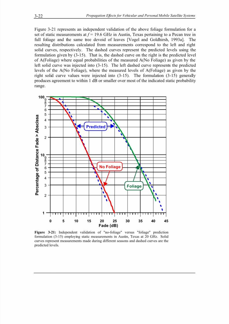
Figure 3-21 represents an independent validation of the above foliage formulation for a
set of static measurements at f = 19.6 GHz in Austin, Texas pertaining to a Pecan tree infull foliage and the same tree devoid of leaves [Vogel and Goldhirsh, 1993a]. The
resulting distributions calculated from measurements correspond to the left and rightsolid curves, respectively. The dashed curves represent the predicted levels using the
formulation given by (3-15). That is, the dashed curve on the right is the predicted levelof A(Foliage) where equal probabilities of the measured A(No Foliage) as given by the
left solid curve was injected into (3-15). The left dashed curve represents the predictedlevels of the A(No Foliage), where the measured levels of A(Foliage) as given by the
right solid curve values were injected into (3-15). The formulation (3-15) generally produces agreement to within 1 dB or smaller over most of the indicated static probability
range.
0 5 10 15 20 25 30 35 40 45
Fade (dB)
2
3
4
5
6789
2
3
4
5
6789
1
10
100
P e r c e n t a g e o
f D i s t a n c e F a d e > A b s c i s s a
Foliage
No Foliage
Predicted
Figure 3-21: Independent validation of "no-foliage" versus "foliage" prediction
formulation (3-15) employing static measurements in Austin, Texas at 20 GHz. Solid
curves represent measurements made during different seasons and dashed curves are the
predicted levels.
7/18/2019 Road side tree RF attenuation
http://slidepdf.com/reader/full/road-side-tree-rf-attenuation 29/42
Attenuation Due to Roadside Trees: Mobile Case 3-23
3.5.2 UHF (870 MHz)
In Chapter 2 it was shown that a 35% increase in the dB attenuation was experienced at870 MHz when comparing attenuation from trees having no foliage and those having
foliage (winter versus summer) for the static measurement case. This case correspondedto a configuration in which the vehicle was stationary and the propagation path
intersected the canopy. Seasonal measurements employing a helicopter as the transmitter platform were also performed by the authors for the dynamic case in which the vehicle
traveled along a tree-lined highway in Central Maryland (Route 295) along which the propagation path was shadowed over approximately 75% of the road distance [Goldhirsh
and Vogel, 1987; 1989]. Cumulative fade distributions obtained from measurements inOctober 1985 (trees with leaves) and in March 1986 (trees without leaves) are shown in
Figure 3-22. The results demonstrate the following:
At f = 870 MHz, 1% 80%≤ ≤ P :
)(24.1)( foliageno A foliage full A = (3-19)
Equation (3-19) states that over the percentage range from 1% to 80% of the seasonalcumulative distributions, there is an average increase of 24% (at equal probability values)
in the dB fade of trees with leaves relative to trees with no leaves. The dB error associated with the above formulation over this percentage range for the curves in Figure
3-22 is less than 0.2 dB. The percentage fade increase (seasonal) for the dynamic case(24%) is less than that for the static case (35%) because the former case represents a
condition in which the optical path is always shadowed, whereas the dynamic case hasassociated with it measurements between trees.
The question arises “Why is there a small difference between the “foliage” and “no-foliage” distributions at UHF (e.g. 24% change), whereas at K-Band, there is a large
change between the distributions for these two scenarios (e.g., two to three times)?” Thisquestion may be answered as follows: The major contributor due to tree attenuation at the
UHF frequency (wavelength of approximately 35 cm) for trees without leaves are the branches, since the separation between contiguous branches along the path are generally
smaller than 35 cm. That is, since the branch separation is generally smaller than awavelength at UHF, no substantial difference exists between the “leaf” and “no-leaf”
cases as both scenarios result in attenuating environments. On the other hand, becausethe K-Band measurements have an associated wavelength of 1.5 cm, the separation
between branches for the “no leaf” case is generally larger than this dimension resultingin a smaller relative fading condition. On the other hand, the “full blossom” case is
highly attenuating at K-Band because of the continuous blockage caused by the high
density of leaves.
7/18/2019 Road side tree RF attenuation
http://slidepdf.com/reader/full/road-side-tree-rf-attenuation 30/42
Propagation Effects for Vehicular and Personal Mobile Satellite Systems3-24
0 1 2 3 4 5 6 7 8 9 10 11 12 13 14 15 16
Fade Depth (dB)
2
3
4
5
6789
2
3
4
5
6789
1
10
100
P e r c e n t a g e o f D i s t a n c e F a d e > A b s c i s s a
October, 1985
March, 1986
Figure 3-22: Cumulative fade distributions at L-Band (1.5 GHz) in central-Maryland
during various seasons.
3.6 Frequency Scaling Considerations
The frequency scaling formulation applied to the ERS model is applicable between UHF(870 MHz) and S-Band (3 GHz) and is given by
for 1% 30%≤ ≤ P and 870 3 MHz f GHz ≤ ≤ :
dB f
f f A f A
L
L )()( = , (3-20)
where GHz f L 5.1= and where )( f A is the attenuation expressed in dB at the frequency
f (expressed in GHz). The frequency scaling in the EERS model is given by exponent
factor in (3-1).
Figure 3-23 depicts a comparison using both frequency scaling formulations and the
measurements of Bundrock and Harvey [1988]. The open circled points correspond tothe formulation (3-20) and the solid points represent the formulation (3-1) with A f L( )
corresponding to the L-Band frequency (1.55 GHz) and attenuation values of Bundrock and Harvey. That is, the estimated points shown were derived from the middle curve
corresponding to the L-Band measured distribution. Since both scaling methods giveapproximately similar results, it is suggested that (3-1) be used for simplicity over the
7/18/2019 Road side tree RF attenuation
http://slidepdf.com/reader/full/road-side-tree-rf-attenuation 31/42
Attenuation Due to Roadside Trees: Mobile Case 3-25
entire frequency range (up to 20 GHz), although both are applicable between UHF and
S-Band.
0 2 4 6 8 10 12 14 16 18 20
Fade Depth (dB)
2
3
4
5
6789
2
3
4
5
6789
1
10
100
P e r c e n t a g e o f D i s t a n c e F a d e > A b s c i s s a
Frequency Scaling Case
ERS Scaling
EERS Scaling
2.66 GHz
0.893 GHz
1.55 GHz
Figure 3-23: Fade distributions at L-Band, S-Band and UHF measured by Bundrock and
Harvey [1988] (solid curves). The open circular and solid circular points represent the
ERS and the EERS frequency scaling estimates, respectively.
3.7 Comparison of EERS Model with Other Empirical Models
3.7.1 Modified Empirical Roadside Shadowing Model (MERS)
This model is an outgrowth of campaigns carried out by the European Space Agency(ESA) [Jongejans et al., 1986] and is described by Sforza et al. [1993a; 1993b] and Butt
et al. [1995]. It is called the Modified Empirical Roadside Shadowing (MERS) and isrepresentative of mobile-satellite attenuation from deciduous trees corresponding to POS
values from 35% to 85%. The formulation has the same form as the ERS model (3-3)and is given by
)()ln()(),( θθθ N P M P A +−= , (3-21)
where
7/18/2019 Road side tree RF attenuation
http://slidepdf.com/reader/full/road-side-tree-rf-attenuation 32/42
Propagation Effects for Vehicular and Personal Mobile Satellite Systems3-26
32
2
1
32
2
1
)(
)(
bbb N
aaa M
++=
++=
θθθ
θθθ, (3-22)
and where
a
a
a
b
b
b
1
4
2
3
1
2
3
1 117 10
0 0701
61304
00032
0 6612
37 8581
== −=== −=
−.
.
.
.
.
.
Χ
(3-23)
In the above, A P ( , )θ is the L-Band (1.5 GHz) fade in dB, P is the percentage of fade
exceeded applicable in the range 1% to 30%, and θ is the elevation angle (in degrees)
valid from 20° to 80°. In Figure 3-24, the above MERS formulation is compared with the
EERS model at 30°, 45°, and 60°. The two models at the different angles generally agreewith one another to approximately 1 dB at the equal percentage levels. The 60° MERS
distribution appears shifted to the right relative to the EERS model by approximately1 dB. Although the above formulation is described for L-Band, it may be used for S-Band frequencies applying the frequency scaling relation (3-20) [Butt et al., 1995].
0 2 4 6 8 10 12 14 16 18 20 22 24
Fade Depth (dB)
2
3
4
5
6789
2
3
4
5
6789
1
10
100
P e r c e n t a g e o f t h e T i m e F a d e > A b s c i s
s a
30°
45°
60°
Figure 3-24: Comparison of EERS model (solid) with MERS (dashed) results at L-Band
(1.5 GHz).
7/18/2019 Road side tree RF attenuation
http://slidepdf.com/reader/full/road-side-tree-rf-attenuation 33/42
Attenuation Due to Roadside Trees: Mobile Case 3-27
3.7.2 Empirical Fading Model (EFM)
This model was derived from measurements made by the Centre for Satellite Engineeringat the University of Surrey, UK. It is based on simultaneous measurements at L, S, and
K u bands at the higher elevation angles from 60° to 80° [Butt et al., 1993; 1995]. Thismodel also has a form similar to the ERS model (3-3) and is given by
N P M f P A +−= )ln(),,( θ (3-24)
with
374.21483.1129.0
315.6182.0029.0
++−=++−=
f N
f M
θ
θ(3-25)
and where A P f ( , , )θ is the attenuation (in dB) at the percentage P (in %) valid from 1%
to 20%, θ is the elevation angle (in degrees) applicable from 60° to 80°, and the
frequency f (in GHz) may be applied in the range 1.3 GHz to 10.4 GHz. The
multiplying constants on the right hand side of M in (3-25) are the negative of those
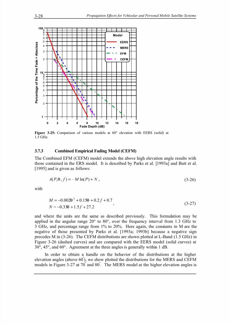
presented by Butt et al. [1993, 1995] because M in (3-24) is preceded by a negative signto maintain consistency with the EERS model. (Their multiplying coefficient was positive). Figure 3-25 shows a comparison of the above model distribution at 60°
elevation with those corresponding to the EERS, MERS, and CEFM (to be describedshortly). It is interesting to note that the other three models cluster about one another,
whereas the EFM model deviates considerably from the grouping; especially at percentages smaller than 5%.
7/18/2019 Road side tree RF attenuation
http://slidepdf.com/reader/full/road-side-tree-rf-attenuation 34/42
Propagation Effects for Vehicular and Personal Mobile Satellite Systems3-28
0 2 4 6 8 10 12 14 16 18
Fade Depth (dB)
2
3
4
5
6789
2
3
4
5
6789
1
10
100
P e r c e n t a g e o f t h e T i m e F a d e >
A b s c i s s a
Model
EERS
MERS
EFM
CEFM
Figure 3-25: Comparison of various models at 60° elevation with EERS (solid) at
1.5 GHz.
3.7.3 Combined Empirical Fading Model (CEFM)
The Combined EFM (CEFM) model extends the above high elevation angle results withthose contained in the ERS model. It is described by Parks et al. [1993a] and Butt et al.
[1995] and is given as follows:
N P M f P A +−= )ln(),,( θ , (3-26)
with
2.275.133.0
7.02.015.0002.02
++−=+++−=
f N
f M
θ
θθ, (3-27)
and where the units are the same as described previously. This formulation may be
applied in the angular range 20° to 80°, over the frequency interval from 1.3 GHz to
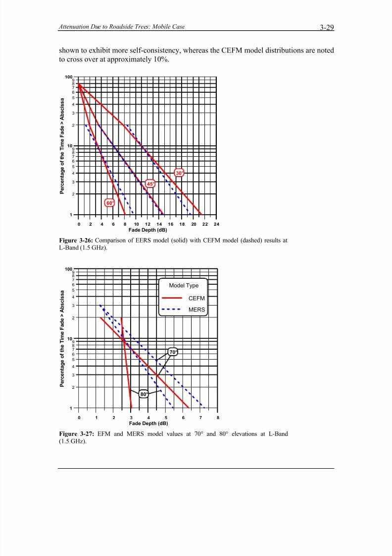
3 GHz, and percentage range from 1% to 20%. Here again, the constants in M are thenegative of those presented by Parks et al. [1993a; 1993b] because a negative sign precedes M in (3-26). The CEFM distributions are shown plotted at L-Band (1.5 GHz) in
Figure 3-26 (dashed curves) and are compared with the EERS model (solid curves) at30°, 45°, and 60°. Agreement at the three angles is generally within 1 dB.
In order to obtain a handle on the behavior of the distributions at the higher elevation angles (above 60
°), we show plotted the distributions for the MERS and CEFM
models in Figure 3-27 at 70° and 80
°. The MERS model at the higher elevation angles is
7/18/2019 Road side tree RF attenuation
http://slidepdf.com/reader/full/road-side-tree-rf-attenuation 35/42
Attenuation Due to Roadside Trees: Mobile Case 3-29
shown to exhibit more self-consistency, whereas the CEFM model distributions are noted
to cross over at approximately 10%.
0 2 4 6 8 10 12 14 16 18 20 22 24
Fade Depth (dB)
2
3
4
5
6
7
89
2
3
4
5
6
7
89
1
10
100
P e r c e n t a g e o f t h e T i m e F a d e > A b s c i s s a
30°
45°
60°
Figure 3-26: Comparison of EERS model (solid) with CEFM model (dashed) results at
L-Band (1.5 GHz).
0 1 2 3 4 5 6 7 8
Fade Depth (dB)
2
3
4
5
6789
2
3
45
6789
1
10
100
P e r c e n t a g e o f t h e T i m e F a d e > A b s c i s s a
Model Type
CEFM
MERS
70°
80°
Figure 3-27: EFM and MERS model values at 70° and 80° elevations at L-Band
(1.5 GHz).
7/18/2019 Road side tree RF attenuation
http://slidepdf.com/reader/full/road-side-tree-rf-attenuation 36/42
Propagation Effects for Vehicular and Personal Mobile Satellite Systems3-30
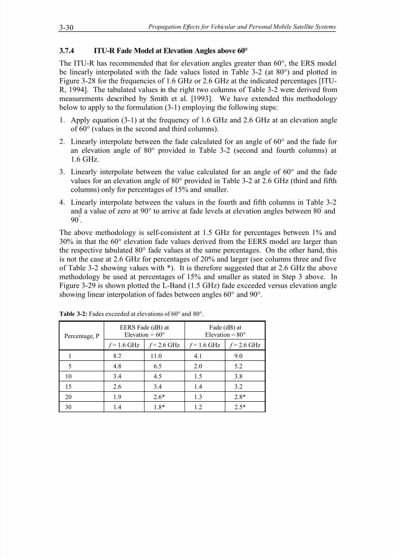
3.7.4 ITU-R Fade Model at Elevation Angles above 60°
The ITU-R has recommended that for elevation angles greater than 60°, the ERS model be linearly interpolated with the fade values listed in Table 3-2 (at 80°) and plotted in
Figure 3-28 for the frequencies of 1.6 GHz or 2.6 GHz at the indicated percentages [ITU-R, 1994]. The tabulated values in the right two columns of Table 3-2 were derived from
measurements described by Smith et al. [1993]. We have extended this methodology below to apply to the formulation (3-1) employing the following steps:
1. Apply equation (3-1) at the frequency of 1.6 GHz and 2.6 GHz at an elevation angleof 60° (values in the second and third columns).
2. Linearly interpolate between the fade calculated for an angle of 60° and the fade for an elevation angle of 80° provided in Table 3-2 (second and fourth columns) at
1.6 GHz.
3. Linearly interpolate between the value calculated for an angle of 60° and the fade
values for an elevation angle of 80° provided in Table 3-2 at 2.6 GHz (third and fifthcolumns) only for percentages of 15% and smaller.
4. Linearly interpolate between the values in the fourth and fifth columns in Table 3-2and a value of zero at 90° to arrive at fade levels at elevation angles between 80 ° and
90°.
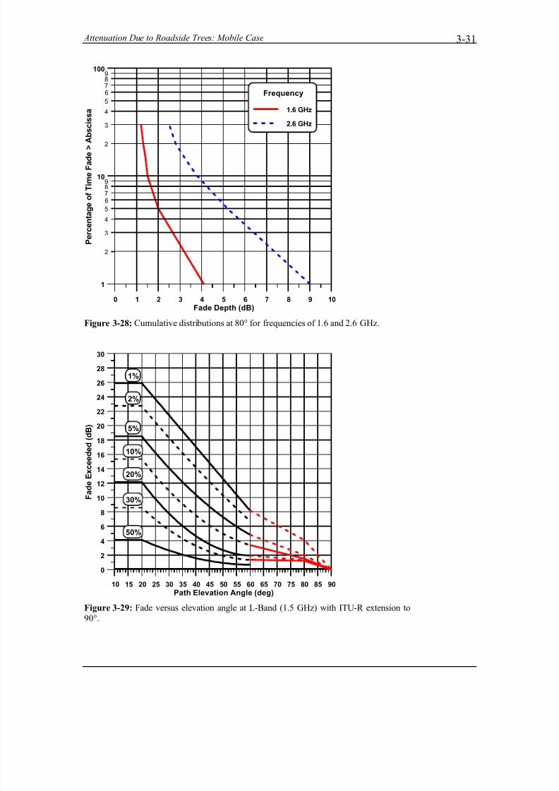
The above methodology is self-consistent at 1.5 GHz for percentages between 1% and
30% in that the 60° elevation fade values derived from the EERS model are larger thanthe respective tabulated 80° fade values at the same percentages. On the other hand, this
is not the case at 2.6 GHz for percentages of 20% and larger (see columns three and fiveof Table 3-2 showing values with *). It is therefore suggested that at 2.6 GHz the above
methodology be used at percentages of 15% and smaller as stated in Step 3 above. InFigure 3-29 is shown plotted the L-Band (1.5 GHz) fade exceeded versus elevation angle
showing linear interpolation of fades between angles 60° and 90°.
Table 3-2: Fades exceeded at elevations of 60° and 80°.
EERS Fade (dB) atElevation = 60°
Fade (dB) atElevation = 80°Percentage, P
f = 1.6 GHz f = 2.6 GHz f = 1.6 GHz f = 2.6 GHz
1 8.2 11.0 4.1 9.0
5 4.8 6.5 2.0 5.2
10 3.4 4.5 1.5 3.8
15 2.6 3.4 1.4 3.2
20 1.9 2.6* 1.3 2.8*
30 1.4 1.8* 1.2 2.5*
7/18/2019 Road side tree RF attenuation
http://slidepdf.com/reader/full/road-side-tree-rf-attenuation 37/42
Attenuation Due to Roadside Trees: Mobile Case 3-31
0 1 2 3 4 5 6 7 8 9 10
Fade Depth (dB)
2
3
4
5
6789
2
3
4
5
6789
1
10
100
P e r c e n t a g e o f T i m e F a d e > A b s c i s s a
Frequency
1.6 GHz
2.6 GHz
Figure 3-28: Cumulative distributions at 80° for frequencies of 1.6 and 2.6 GHz.
10 15 20 25 30 35 40 45 50 55 60 65 70 75 80 85 90
Path Elevation Angle (deg)
0
2
4
6
8
10
12
14
16
18
20
22
24
26
28
30
F a d e E x c e e d e d ( d B )
1%
2%
5%
10%
20%
30%
50%
Figure 3-29: Fade versus elevation angle at L-Band (1.5 GHz) with ITU-R extension to
90°.
7/18/2019 Road side tree RF attenuation
http://slidepdf.com/reader/full/road-side-tree-rf-attenuation 38/42
Propagation Effects for Vehicular and Personal Mobile Satellite Systems3-32
3.7.5 Comparative Summary of Model Limits
In Table 3-3 is given a comparative summary of the above competing models and their domains of validity. The EERS model covers a wider range of percentages than the other
models (1% to 80%) and includes angles as low as 7°. The other models are limited to20° elevation. It also covers the greatest range of frequencies (e.g., 0.87 to 20 GHz). The
EERS model limitation vis-à-vis the other models is that it does not include elevationangles greater than 60°. The ITU-R model extends the EERS model from 60° to 90° at
1.6 GHz and 2.6 GHz. The EFM, CEFM, and MERS models include elevation angles upto 80°.
Table 3-3: Summary of empirical models and their domains of validity.
Model NamePercentageRange (%)
Elevation AngleRange (deg)
Frequency Range(GHz)
Reference
EERS 1-80 7-60 0.87-20Goldhirsh and Vogel
[1995a], ITU-R [1997]
ERS 1-20 20-60 0.87-3 Goldhirsh and Vogel[1992], ITU-R [1994]
ITU-R 1-30 60-90 1.6-2.6 ITU-R [1997]
EFM 1-20 60-80 1.3-10.4 Parks et al. [1993a]
MERS 1-30 20-80 1.5-2.6 Sforza et al. [1993a]
CEFM 1-20 20-80 1.5-2.6 Butt et al. [1995]
3.8 Conclusions and Model Recommendations
The following is recommended:
1. In the elevation angle interval between 20° to 60°, the EERS model should be
executed as outlined in Section 3.3.2 using the step by step approach in Section 3.3.3.The ITU-R angle extension procedure from 60° to 90° may be used at 1.6 GHz and
2.6 GHz as outlined in Section 3.7.4. The MERS model (Equation (3-21) and Figure3-24) and the CEFM model (Equation (3-26) and Figure 3-26) show relatively small
differences with the EERS model in the angular range 20° to 60°.
2. For elevation angles between 7° and 20° the EERS model should continue to be
employed in the absence of any direct measurements. The model provides a medianof measured distributions at the smaller angles, but the deviation from the measured
levels may be significantly larger than 5 dB at equal probability levels because of
terrain blockage and multiple canopy tree-shadowing. Where direct measurementsexist, these should be substituted for the model.
7/18/2019 Road side tree RF attenuation
http://slidepdf.com/reader/full/road-side-tree-rf-attenuation 39/42
Attenuation Due to Roadside Trees: Mobile Case 3-33
3.9 References
Bundrock, A. and Harvey, R. [1988], “Propagation Measurements for an Australian LandMobile Satellite System,” Proceedings of International Mobile Satellite Conference,Pasadena, CA, pp. 119-124.
Butt, G., B. G. Evans, M. Parks [1995], “Modeling the Mobile Satellite Channel for Communication System Design,” Ninth International Conference on Antennas and Propagation,” 4-7 April, 1995, pp. 387-393.
Butt, G., B. G. Evans, M. Richharia [1993], “Results of Multiband (L, S, Ku BandPropagation Measurements for High Elevation Angle Land Mobile Satellite
Channel,” Eighth International Conference on Antennas and Propagation, 30March-2 April, 1993, Herriot-Watt University, U.K., pp. 796-799 (Institution of Electrical Engineers, London, Conference Publication 370.)
Goldhirsh, J. and W. J. Vogel [1995a], “An Extended Empirical Roadside ShadowingModel for Estimating Fade Distributions from UHF to K Band for Mobile Satellite
Communications,” Space Communications (Special Issue on Satellite Mobile and
Personal Communications), Vol. 13, No. 3 (IOS Press).Goldhirsh, J. and W. J. Vogel [1995b], “Extended Empirical Roadside Shadowing Model
from ACTS Mobile Measurements,” Proceedings of the Nineteenth NASA
Propagation Experimenters Meeting (NAPEX XIX) and the Seventh Advanced Communications Technology Satellite (ACTS) Propagation Studies Workshop
(APSW VII), Fort Collins, Colorado, June 14-16, pp. 91-101. (JPL Publication 95-15, Jet Propulsion Laboratory, California Institute of Technology, Pasadena,California.)
Goldhirsh, J., W. J. Vogel, and G. W. Torrence [1995], “Mobile PropagationMeasurements in the U.S. at 20 GHz Using ACTS,” International Conference on
Antennas and Propagation (ICAP ‘95), Vol. 2, Conference Publication No. 407,
Eindhoven, The Netherlands, pp. 381-386.
Goldhirsh, J., W. J. Vogel, and G. W. Torrence [1994], “ACTS Mobile Propagation
Campaign,” Proceedings of the Eighteenth NASA Propagation Experimenters Meeting (NAPEX XVIII) and the Advanced Communications Technology Satellite
(ACTS) Propagation Studies Miniworkshop, Vancouver, British Columbia, June 16-17, 1994, pp. 135-150. (JPL Publication 94-19, Jet Propulsion Laboratory, CaliforniaInstitute of Technology, Pasadena, California.)
Goldhirsh, J. and W. J. Vogel [1992], “Propagation Effects for Land Mobile SatelliteSystems: Overview of Experimental and Modeling Results,” NASA Reference
Publication 1274, (Office of Management, Scientific and Technical InformationProgram), February.
Goldhirsh, J. and W. J. Vogel [1989], “Mobile Satellite System Fade Statistics for
Shadowing and Multipath from Roadside Trees at UHF and L Band,” IEEE Transactions on Antennas and Propagation, Vol. AP-37, No. 4, April, pp. 489-498.
Goldhirsh, J. and W. J. Vogel [1987], “Roadside Tree Attenuation Measurements at UHF
for Land-Mobile Satellite Systems,” IEEE Transactions on Antennas and Propagation, Vol. AP-35, pp. 589-596, May.
7/18/2019 Road side tree RF attenuation
http://slidepdf.com/reader/full/road-side-tree-rf-attenuation 40/42
Propagation Effects for Vehicular and Personal Mobile Satellite Systems3-34
ITU-R [1994] (International Telecommunication Union, Radio Communication Study
Groups), “Propagation Data Required for the Design of Earth-Space Land MobileTelecommunication Systems,” Recommendation ITU-R PN.681-1, International
Telecommunication Union, ITU-R Recommendations, 1994 PN Series Volume,Propagation in Non-Ionized Media, pp. 358-365.
ITU-R [1997] (International Telecommunications Union, Radio Communication StudyGroups, “Revision of Recommendation ITU-R P.681,” Document 3M/3 - February.
Joanneum Research [1995], “Land Mobile Satellite Narrowband Propagation Campaignat Ka Band,” Final Report W.O. #4, ESTEC Contract 9949/92/NL, January.
Jongejans, A., A. Dissanayake, N. Hart, H. Haugli, C. Loisy, and R. Rogard [1986],
“PROSAT-Phase 1 Report,” European Space Agency Tech. Rep. ESA STR-216,May. (European Space Agency, 8-10 Rue Mario-Nikis, 75738 Paris Cedex 15,France.)
Murr, F., B. Arbesser-Rastburg, S. Buonomo, Joanneum Research [1995], “Land MobileSatellite Narrowband Propagation Campaign at Ka Band,” International MobileSatellite Conference (IMSC ’95), Ottawa, Canada, pp. 134-138.
Paraboni, A. and B. Giannone, [1991], “Information for the participation to theITALSAT Propagation Experiment,” Politecnico di Milano Report 91.032.
Parks, M. A. N., G. Butt, and B. G. Evans [1993a], “Empirical Models Applicable to
Land Mobile Satellite System Propagation Channel Modeling,” Colloquium onCommunications Simulation and Modeling Techniques, London, England, pp. 12/1-
12/6. (The Institution of Electrical Engineers, Savoy Place, London, WC2R OBL,UK.)
Parks, M. A. N., G. Butt, B. G. Evans, M. Richharia [1993b], “Results of Multiband (L,
S, Ku Band) Propagation Measurements and Model for High Elevation Angle LandMobile Satellite Channel ,” Proceedings of XVII NAPEX Conference, June 14th -15th,
Pasadena, California, pp. 193-202. (JPL Publication 93-21; Jet PropulsionLaboratory, California Institute of Technology, Pasadena, California.)
Sforza, M., S. Buonomo, J. P. V. Poiares Baptista [1993a], “Global Coverage Mobile
Satellite Systems: System Availability versus Channel Propagation Impairments,”IMCS ’93, June, pp. 361-372.
Sforza, M. and S. Buonomo [1993b], “Characterization of the LMS Propagation Channel
at L- and S- Bands: Narrowband Experimental Data and Channel Modeling,” Proceedings of XVII NAPEX Conference, June 14
th-15
th, Pasadena, California, pp.
183-192. (JPL Publication 93-21; Jet Propulsion Laboratory, California Institute of Technology, Pasadena, California.)
Smith, H., J. G. Gardiner, and S. K. Barton [1993], “Measurements on the Satellite-Mobile Channel at L & S Bands,” Proceedings of the Third International MobileSatellite Conference (IMSC ’93), June 16-18, Pasadena, California, pp. 319-324.
Vogel, W. J., G. W. Torrence, and J. Goldhirsh [1994], “ACTS 20 GHz Mobile
Propagation Campaign in Alaska,” Presentations of the Sixth ACTS PropagationStudies Workshop,” Clearwater Beach, Florida, November 28-30, pp. 283-294. (JPL
Technical Report JPL D-12350, December 1994, Jet Propulsion Laboratory,California Institute of Technology, Pasadena, California.)
7/18/2019 Road side tree RF attenuation
http://slidepdf.com/reader/full/road-side-tree-rf-attenuation 41/42
Attenuation Due to Roadside Trees: Mobile Case 3-35
Vogel, W. J. and J. Goldhirsh [1993a], “Earth-Satellite Tree Attenuation at 20 GHz:
Foliage Effects,” Electronics Letters, Vol. 29, No. 18, 2nd September, 19, pp.1640-1641.
Vogel, W. J. and J. Goldhirsh [1995], “Multipath Fading at L Band for Low Elevation
Angle, Land Mobile Satellite Scenarios,” IEEE Journal on Selected Areas in
Communications, Vol. 13, No. 2, February, pp. 197-204.Vogel, W. J. and J. Goldhirsh [1993b], “Tree Attenuation at 20 GHz: Foliage Effects,”
Proceedings of the Seventeenth NASA Propagation Experimenters Meeting (NAPEX XVII) and the Advanced Communications Technology Satellite (ACTS) Propagation
Studies Miniworkshop,” Pasadena, California, June 14-15, pp. 219-223. (JPLPublication 93-21, Jet Propulsion Laboratory, California Institute of Technology,Pasadena, California.)
Vogel, W. J., J. Goldhirsh, and Y. Hase [1992], “Land-Mobile-Satellite FadeMeasurements in Australia,” AIAA Journal of Spacecraft and Rockets, Vol. 29, No.1, Jan-Feb, pp. 123-128.
Vogel, W. J. and J. Goldhirsh [1990], “Mobile Satellite System PropagationMeasurements at L Band Using MARECS-B2,” IEEE Transactions on Antennas and Propagation, Vol. AP-38, No. 2, February, pp. 259-264.

7/18/2019 Road side tree RF attenuation
http://slidepdf.com/reader/full/road-side-tree-rf-attenuation 42/42


![Accuracy and interpretability, tree-based machine learning ... · We consider the single regression tree (ST) method along with 3 tree ensemble methods: random forests (RF) [7], extremely](https://img.pdfslide.us/doc/110x75/5f58ac3258d7c4057950489d/accuracy-and-interpretability-tree-based-machine-learning-we-consider-the-single.jpg)