Revisiting Gertler-Gilchrist Evidence on the Behavior of Small and

FEDERAL RESERVE BANK OF SAN FRANCISCO

WORKING PAPER SERIES

Revisiting the Behavior of Small and Large Firms during the 2008 Financial Crisis

Marianna Kudlyak

Federal Reserve Bank of San Francisco

Juan M. Sanchez Federal Reserve Bank of St. Louis

December 2016

Working Paper 2016-22

http://www.frbsf.org/economic-research/publications/working-papers/wp2016-22.pdf

Suggested citation:

Kudlyak, Marianna, Juan M. Sanchez. 2016. “Revisiting the Behavior of Small and Large Firms during the 2008 Financial Crisis” Federal Reserve Bank of San Francisco Working Paper 2016-22. http://www.frbsf.org/economic-research/publications/working-papers/wp2016-22.pdf The views in this paper are solely the responsibility of the authors and should not be interpreted as reflecting the views of the Federal Reserve Bank of San Francisco or the Board of Governors of the Federal Reserve System.

http://www.frbsf.org/economic-research/publications/working-papers/wp2016-22.pdf

Revisiting the Behavior of Small and Large Firms during the

2008 Financial Crisis

Marianna Kudlyak Federal Reserve Bank of San Francisco

[email protected]

Juan M. Sanchez Federal Reserve Bank of St. Louis

[email protected]

This Draft: December 22, 2016

First Draft: April 27, 2010

Gertler and Gilchrist (1994) provide seminal evidence for the prevailing view that adverse shocks are propagated via credit constraints. Under this view, the deep recession that followed the 2008 financial crisis is often interpreted as the propagation of the initial “credit shock.” Following Gertler and Gilchrist (1994)’s methodology, we study the behavior of small and large firms during the episodes of credit disruption and extend the analysis to the 2008 financial crisis and NBER-dated recessions. We find that large firms' short-term debt and sales contracted relatively more than those of small firms during the 2008 financial crisis and during most recessions since 1969. These results, which we show are robust to changes in the business cycle dating procedure, suggest that an alternative view may be needed to understand the prolonged recession following the 2008 financial crisis.

JEL: E52, E51, E32. Keywords: Small and Large firms. Credit Constraints. Propagation of Shocks. Leverage.

The views expressed here do not necessarily reflect those of the Federal Reserve Bank of San Francisco, the Federal Reserve Bank of St. Louis, or the Federal Reserve System. We thank Marisa Reed, Devin Reilly, David Min, and Constanza S. Liborio for excellent research assistance. All errors are ours alone.

mailto:[email protected]

mailto:[email protected]

2

1. Introduction

The propagation of shocks into large economic disturbances is a long-standing puzzle in

macroeconomic analysis. The financial accelerator models provide one such mechanism of

propagation (Bernanke, Gertler, and Gilchrist, 1996, 1999).1 In such models, adverse conditions

in credit markets curtail the economic activity by impacting sales, inventories, and, eventually,

employment. The implication of the mechanism is that firms whose credit is the most vulnerable

to the disruptions in the credit markets are the first to bear the negative impact of the adverse shock

to the economy. In a seminal work, Gertler and Gilchrist (1994) provide evidence that serves as a

basis for the prevailing view that the adverse shocks are propagated via small firms’ constraints in

the access to capital markets; that is, the financial accelerator mechanism works via credit

constraints of small firms.

In this article, we revisit the question of the differences in behavior between small and large

manufacturing firms during the 2007-09 economic crisis, which is largely believed to be a period

when credit becomes more costly or harder to obtain and is also the period of the Great Recession

that turned out to be one of the longest recessions during the postwar period. Using the same dataset

as in the work by Gertler and Gilchrist (1994), we, first, replicate Gertler and Gilchrist results; we

then analyze the behavior of short-term debt, sales, and inventories of firms, extending the period

under study to the 2007-09 recession and specifically focusing on the aftermath of the financial

markets turmoil in the third quarter of 2008; and, finally, we examine the behavior of the growth

rates around NBER-dated recession peaks.

The evidence for the prevailing view comes from seminal work of Gertler and Gilchrist

(1994) who use the Quarterly Financial Report for Manufacturing, Mining, and Wholesale Trade

(henceforth QFR), which provides financial data on both publicly and privately held firms grouped

by asset size. They study the behavior of small and large manufacturing firms around the five

episodes of contractionary monetary policy (1968, 1974, 1978, 1979, and 1988) and an episode of

credit crunch (1966) in the postwar period. Gertler and Gilchrist find that immediately following

a tight money date, small firms' holdings of short-term debt decline while those of large firms rise.

The sales and inventories of small firms, moreover, decline much more than those of large firms.

1 See a critical review in Smant (2002).

3

Gertler and Gilchrist interpret the results as suggesting that large firms enjoy easier access to credit,

and that their access to credit enables them to borrow to carry inventories in spite of credit market

shocks. Oliner and Rudebush (1996a, 1996b) also use QFR and find that during 1974-1991

monetary contractions induce a shift in total lending away from small firms.2

We start by replicating the findings of Gertler and Gilchrist (1994) for the periods prior to

1990 and for an additional tight money episode that we identify – the second quarter of 1994. We

then seek to determine whether these findings could be reproduced in the context of the turmoil in

the economy after September 2008, which is marked by the collapse of Lehman Brothers Inc. and

is widely characterized by substantial disruptions in credit markets.3 Surprisingly, we find that

following the third quarter of 2008, short-term debt and sales of large firms declined much more

than those of small firms, in contrast to the prevailing view regarding the behavior of large versus

small firms during previous episodes of tight money. Specifically, the short-term debt of large

firms decreased from its peak by more than twice as much as that of small firms. This decrease in

short-term debt was also associated with a substantially larger decline of sales for large firms as

compared to small firms. This finding is robust to alternative methods used to determine the timing

of the growth rate changes around the episode.

The crisis that erupted after the third quarter of 2008 closely follows the beginning of the

NBER-dated 2007-09 recession (December 2007). Consequently, while on the surface the events

surrounding the third quarter of 2008 might appear as resulting from a credit or tight money shock,

it might be that these events are a manifestation of other types shocks, responsible for the Great

Recession. To understand whether our findings regarding the 2007-09 recession are specific to this

episode or are rather reminiscent of the earlier recessions, we examine the behavior of small and

large firms around previous recessions. We find that in all recessions from 1969 to 2009, the short-

term debt growth for large firms declined more than that of small firms. In the 2007-09 and the

2 Recently, Tenreyro and Thwaites (forthcoming) study the effect of monetary policy on the U.S. economy using monetary policy shocks as identified by Romer and Romer (2004) and extended by Coibon (2012). Gilchrist and Zakrajsek (2012) examine the effect of financial shocks as measured by the excess bond premium. 3 In April 2010, Christina Romer wrote: "The recent recession was obviously not caused by tight monetary policy. Interest rates were not especially high when it began, and so the Federal Reserve had only limited room to cut them ... That is, despite the very low level of interest rates and all the attention to the growth of the Federal Reserve's balance sheet, current monetary policy is in fact unusually tight given the condition of the economy" (Romer, 2010).

4

2001 recessions, the growth rates of sales and inventories of large firms also declined more than

that of small firms. Consequently, the behavior of small versus large firms around the 2007-09

economic crisis closer resembles the behavior of firms around previous recessions than around

earlier tight money episodes.

Our finding that after the third quarter of 2008 large firms contracted much more than small

firms thus is not consistent with the predictions of the financial accelerator models’ response to

tight money or credit crunch shocks (for example, Bernanke, Gertler, and Gilchrist, 1999 and

Kiyotaki and Moore, 1997). There are a few possible interpretations for our findings. First, it might

be the case that small versus large firm is not a good approximation of the debt-constrained versus

unconstrained dimension for firms. Alternatively, it might be that the 2007-09 period was not a

period of “tight money,” i.e., a tightening of a financial or collateral constraint is not a good

representation of the 2007-09 recession. Rather, the shock (or a combination of shocks) associated

with the 2007-09 recession might primarily propagate via large firms. Given that a large literature

provides evidence that small firms are actually more credit constrained than the large firms, we

believe that the latter hypothesis may be responsible for our findings.

Our findings are also consistent with the emerging literature on the propagation of shocks

during the 2007-09 crisis. In a recent work, Moscarini and Postel-Vinay (2012) finds that in the

1990 and the 2001 recessions, large firms were hit particularly hard in terms of employment.4

Interestingly, pre-war evidence also shows that large firms suffered more than small firms during

crises. In particular, King (1923) finds that small firms experienced a smaller decrease in

employment during the 1920-21 recession.5 Closer to our study, Chari, Christiano, and Kehoe

(2013) study the behavior of sales of small and large firms around the postwar recessions prior to

2000 and their results are broadly consistent with ours. 6 Recently, a number of papers emphasize

4 See, however, Fort, Haltiwanger, Jarmin, and Miranda (2013) on the cyclical sensitivity of firms by age and size. 5 We thank Mark Bils for pointing to us this evidence. 6 Recently, in an article published by the Federal Reserve Bank of New York, Sahin, Kitao, Coroaton, and Laiu (2011) argue that small businesses experienced disproportionate job losses during the 2007-09 recession. Using the QFR data, they consider a nominal threshold of $50 million to define small firms, which makes a comparison with Gertler and Gilchrist (1994) and our results difficult because the nominal threshold captures a decreasing fraction of the firm distribution over time. Using this nominal threshold for small firms, they find that, in terms of debt, the debt of large firms does not decline until the financial crisis,

5

a large role of large firms in propagation of shocks. For example, Barlevy (2003) proposes a model

in which firms that are more dependent on external financing are more susceptible to credit shocks

as opposed to firms who do not rely on credit because they do not have access to it. For example,

large firms by having a greater access to credit and thus being more dependent on external

financing might be more negatively impacted during periods of credit crunch.7 Recently, Giroud

and Mueller (2015) argue that firms’ balance sheets were instrumental in the propagation of shocks

during the 2007-09. They show that high-leverage firms exhibit a significantly larger decline in

employment in response to demand shocks than low-leverage firms.8 Gilchrist, Schoenle, Sim,

and Zakrajsek (2015) study price behavior of firms with and without liquidity constraints and find

that high liquidity constraint firms experienced larger drop in their prices during the 2007-09

period.9 In our data set, the limited information on leverage that is available indicates that small

firms are actually more leveraged than large firms, although the difference is rather small.

The remainder of the paper is organized as follows. Section 2 describes the data and

construction of the series. Section 3 provides a descriptive analysis of the series. Section 4 provides

empirical results from periods of tight money dates. Section 5 provides empirical results from

recessions. Section 6 concludes.

2. Data and Construction of the Series

In this section, we describe the data and construction of the growth rate series for small and

large firms. We use the same dataset as the one used by Gertler and Gilchrist (1994) and closely

follow their methodology for constructing the series from the raw data.

while the debt of small firms starts decreasing earlier. In terms of sales, their results on the decline from peak to trough is in line with our results: the decline is larger for large business. 7 Barlevy (2003) proposes a theory of sullying effect of recessions. Foster, Grim and Haltiwanger (2016) find evidence in favor of Barlevy’s hypothesis during the 2007-09 recession. Specifically, they find that in the 2007-09 recession, the intensity of reallocation fell rather than rose and the reallocation that did occur was less productivity enhancing than in prior recessions. 8 See also Herrera, Kolar, and Minetti (2011) for a study credit reallocation across firms. 9 Other recent works on the role of small and large firms in the propagation of shocks include Siemer (2014), Duygan-Bump, Levkov, and Montoriol-Garriga (2015), Mehrotra and Sergeyev (2016), Abo-Zaid and Zervou (2016), and Adelino, Ma, and Robinson (forthcoming).

6

2.1. The Quarterly Financial Report Data

The data in the analysis are from the Quarterly Financial Report for Manufacturing,

Mining, and Wholesale Trade, which is a Census Bureau quarterly dataset that provides financial

information on various categories of firms. The firm data are aggregated into classes by the firm’s

nominal asset size. There are eight asset classes: assets under $5mln, $5-10mln, $10-25mln, $25-

50mln, $50-100mln, $100-250mln, $250-1000mln, and above $1000mln. Each financial series are

thus available by the firm asset size class. We use quarterly data for all manufacturing firms from

the fourth quarter of 1958 to the second quarter of 2014. In the analysis, we use only data on

manufacturing firms because the data on manufacturing firms are available by asset class going

back to 1950s, which is not the case for other industries, and focusing on manufacturing makes

our analysis easily comparable with the data used by Gertler and Gilchrist.10

We aggregate firms into two groups by asset size - small and large firms - and concentrate

our analysis on these groups. We study the behavior of the growth rates of the three main series -

inventories, sales, and short-term debt of firms, distinguishing between small and large firms by

their asset size.

The main advantage of the dataset is its coverage of both publicly traded and privately held

firms. By contrast, another widely used dataset that contains information on firms, Compustat,

covers only publicly traded companies. The disadvantage of the QFR is that the data on a firm

level are not publicly available and, instead, are aggregated into categories by the firm’s asset size

in nominal terms. The definition of asset size categories remains constant throughout the years.

Consequently, as the distribution of firms by nominal asset size shifts to the right with time, the

lowest nominal class size contains a smaller and smaller percent of the distribution. We thus follow

the Gertler and Gilchrist procedure in assigning the available size classes into our definition of

small and large firms and describe the procedure in detail below. The procedure ensures that,

despite the data are only available by aggregated nominal asset class, the definition of small and

large firms remains consistent over time. Specifically, the procedure designates the firms below

10 Although the share of manufacturing in the economy has been decreasing, the trend has been steady and had started before the start of our sample period. The declining trend is unlikely to explain any difference between our findings and those in Gertler and Gilchrist.

7

the twenty-fifth percentile of each period’s sales distribution as small firms, and the firms above

the twenty-fifth percentile as large.

The QFR data prior to 1988 are available in a form of published quarterly financial reports;

after 1988, the data are available online through the Census. We use the published QFR reports

and manually digitize the data from the 1958-2009 annual reports and use the data from the Census

website for 2010-14.11 In particular, for each quarter, we use the historical QFR publication-

formatted financial data from Tables 34, 35, 72, 74, 76, 78, and 80. Within these tables, sales are

defined as "Net sales, receipts, and operating revenues." Short-term debt is the sum of all the

components of "short-term debt, original maturity of 1 year or less" within the "Liabilities and

Stockholders' Equity" column. Finally, inventories are listed within the assets column.

2.2. Tight Money Dates

Our main interest is the behavior of the firms’ sales, inventories, and short-term debt series

around two sets of dates. The first set of dates is broadly characterized as the periods of disruption

of credit and which we refer to as tight money dates. The second set of dates refers to the start

dates of recessions as defined by the NBER or NBER-dated peaks.

To define the tight money dates, we closely follow Gertler and Gilchrist (1994), who

identify periods of monetary shocks using the criteria established in Romer and Romer (1988,

1992). These are the periods in which the Federal Reserve attempted not to offset perceived or

prospective increases in aggregate demand but rather to actively shift the aggregate demand curve

back in response to what it perceived to be excessive inflation (Romer and Romer, 1994). To

identify these periods, Romer and Romer examine the FOMC official announcements for the

statements that output would be sacrificed in order to bring down the current level of inflation. As

in the Gertler and Gilchrist work, we also include a credit crunch of 1966 to our list of tight money

dates.

In addition to the dates listed in the Romer and Romer papers and used by Gertler and

Gilchrist in the analysis, we identify a new tight money date that is not covered in the sample

11 The QFR data can be downloaded from http://www.census.gov/econ/qfr/historic.html (see the last two options under the page tab “Historical Data.”) The earlier QFR data that we digitized from the published reports are available for download from goo.gl/ql0dFE.

http://www.census.gov/econ/qfr/historic.html

https://goo.gl/ql0dFE

8

period studied by Gertler and Gilchrist (1994). Following the same criteria as in the original papers,

we determine the second quarter of 1994 to be a tight money date. The FOMC meeting minutes

from August 1994 frequently reference high resource utilization and concerns about greater

inflation: "many of the members commented that the risks of intensifying inflation clearly were

on the upside if the economic expansion did not moderate from its pace in recent quarters." Such

comments in the meeting minutes point to an active attempt by the FOMC to pull back aggregate

demand in light of inflation concerns, which, as noted above, is the criteria Romer and Romer use

to identify monetary shocks.12

2.3. Construction of Growth Rates Series

To construct growth rates from the original QFR data, we create two series - one for small

and one for large firms - of each variable of interest. We define small firms as those that are in the

1st quartile of the firm asset size distribution and large firms as those that are above the 1st quartile

of the asset size distribution. As mentioned above, the QFR data are presented by eight nominal

asset classes-assets under $5mln, $5-10mln, $10-25mln, $25-50mln, $50-100mln, $100-250mln,

$250-1000mln, and above $1000mln. Over time, the definitions of the classes remain unchanged

while the distribution of firms across these classes changes. We thus follow Gertler and Gilchrist

and for each period calculate which asset class out of the eight classes contains the cut-off

percentile for small firms. Using the method that relies on percentiles implies that our definition

of small and large firms does not vary over time.

We then construct the time series for small firms using information from the classes below

the cut-off percentile for small firms plus a weighted share of the class that contains the cut off,

and construct the time series for large firms using information from the classes above the cut-off

percentile plus a weighted share of the class that contains the cut off. Such an approach ensures

that in every period the time series for small firms contain information on firms below the fixed

percentile of the firm distribution and the time series for large firms contain information on firms

from above the fixed percentile.13 Formally, the procedure can be described as follows.

12 We thank Robert Hetzel for helping us to identify this date. See Hetzel (2008) for an in-depth history of monetary policy. 13 That is, while the nominal cut-off for small firms over time might change, the small and large firms always represent the same percentiles of the firms’ distribution.

9

Let ,i ts denote the sales for asset class i in period t , deflated by the GDP deflator. We

create cumulative asset classes, ,i tS , by summing the sales levels for each asset class less than or

equal to i , i.e.,

, ,1

i

i t k tk

S s=

= ∑ .

The growth rate for each cumulative asset class i and period t is

, , 1,

, 1

i t i ti t

i t

S Sg

S−

−

−= .

To construct the growth rates for large and small firms, we set the cutoff percentile for

sales for small firms, 0.25spc = , i.e., small firms are those with sales below the 25th percentile of

sales.14 Note that such an approach ensures that the small firms are always in the first quartile of

the sales distribution.

To designate firms into small- versus large-firm group, we then proceed as follows. For

each cumulative asset class, we calculate the percent of total sales, ,i tSP :

,,

,

i ti t

N t

SSP

S= ,

where N is the number of size classes in the QFR data. We then find the largest cumulative asset

class that contains at most the 25th percentile of total sales. Formally, we find sti such that:

{ } { },1,maxst i t si Ni SP pc∈= < .

14 With time, the cut-off for small firms moves towards higher nominal asset class. We use the 25th percentile instead of the Gertler and Gilchrist (1994) 30th percentile because in 2014 the seven lower nominal asset classes contain 24.14% of the firm distribution and the eighth class contains the rest.

10

We then construct weights for each quarter, stω , such that:

( ), 1,1s s

t t

s ss t ti t i t

pc SP SPω ω+

= + − ,

or,

1,

, 1,

st

s st t

s i tst

i t i t

pc SP

SP SPω +

+

−=

−.

To obtain a growth rate for small firms in period t , we then weight the two growth rates,

,ti tg , and 1,ti tg + , which are the growth rates for the asset class just below the 25th percentile of sales

and for the asset class just above the 25th percentile of sales, respectively.

By analogy, we repeat the procedure for large firms using 1l st tω ω= − to weight the two

corresponding growth rates, the growth rates for the asset class just below the 25th percentile of

sales and for the asset class just above the 25th percentile of sales.

The process for obtaining growth rates of inventories and short-term debt is similar, with

the exception that instead of finding new weights for inventories and short-term debt, we use the

weights and cutoff classes determined from the sales distribution as described above. As in Gertler

and Gilchrist (1994), we use sales rather than output as an indicator of firm activity over time

because we do not have the exact output measure.

Specifically, for inventories, let ,s

t

invi t

g be the growth rate of inventories in the cumulative

asset class just below the 25th percentile of sales, 1,s

t

invi t

g+

be the growth rate of inventories for the

cumulative asset class just above the 25th percentile of sales, and stω be the same weight as above,

then the growth rate of inventories of small firms in period t , ,invt sg , is given by

( ), , 1,1s s

t t

inv s inv s invt s t ti t i t

g g gω ω+

= + − .

11

Once we construct the series of growth rates of sales, short-term debt, and inventories for

small and large firms, we deseasonalize them using a moving average process, linearly detrend the

deseasonalized series, and further filter the detrended series using a Hodrick-Prescott filter with

smoothing parameter 1600, in order to pick up broad trends in the data following Gertler and

Gilchrist (1994). We refer to these series as detrended growth rate series.

2.4. Construction of Changes in Growth Rates

Our main empirical results concern the changes in the growth rates of the respective series

around tight money dates or recessions for small and for large firms. To construct the change of

the growth rate around the period of interest, i.e., around a tight money date or around a start of an

NBER recession, we construct new growth series tG , which is a cumulative growth rate of the

detrended growth rate series from the start of each episode. Formally, for each tight money date or

recession peak, we set 0 0G = and calculate

1t t tG g G −= + .

An important part of the analysis of the changes around the episodes is determining the

timing of the associated peaks and troughs, the values of which are used to calculate the changes

around the episode. We thus employ a few alternative approaches.

First, following Gertler and Gilchrist (1994), we construct the change in the growth rate

following the tight money date by subtracting the values of the series at the tight money date from

the minimum value of the series reached during the twelve quarters following the date. Note that

the periods at which the small firms’ series reach its minimum might differ from the periods at

which the large firms’ series reach its minimum. We examine the sales, inventories, and short-

term debt series for small and for large firms by hand to determine such minimums.

Second, as we show below, the growth rate series often continue growing after tight money

dates. We thus present a second set of results for the change in the growth series following tight

money dates calculating the peak of the series not at the tight money date but at the closest peak if

the series keep growing following the date.

12

Third, we observe that often large firms’ growth rates continue falling past the twelve

quarters after a tight money date. We thus employ a third procedure for calculating the change in

the growth rates following the tight money date by defining the trough as the lowest value of the

series after the peak without a 12-quarter constraint.15

Finally, since Gertler and Gilchrist do not examine the recession episodes, we set the peaks

and troughs around recession episodes as follows. For the NBER-peaks (whereby an NBER-peak

identifies the start of a recession), we observe that the series often continue growing for a few more

quarters after the NBER-peak. We thus find the peak value of tG reached at or immediately

following the quarter of the NBER-peak and find the minimum following this peak, within at most

twelve quarters since the NBER-peak. Formally, for each NBER-peak, *t , the peak value of tG

is given by

{ }*

* *

12

,max t

tPeak t tG G += ,

and the trough value is identified as the minimum value following the peak value, i.e.,

{ }*

* *,p

12

,min t

tTrough t tG G += ,

where *, pt is the quarter in which the peak value, *,, pPeak tG , is reached. The change in the growth

rate following a recession peak is then the difference between the peak and trough values following

each episode. This approach coincides with our second approach above for the tight money dates.

Note that to determine peaks and troughs, we examine each series for small and for large firms

separately. The periods when the respective series reach its peaks and subsequent troughs for small

firms do not necessary coincide with the peaks and troughs for large firms.

3. Descriptive Time-Series Analysis

15 Note that the periods when the respective series reach its peaks and subsequent troughs for small firms do not necessary coincide with the peaks and troughs for large firms

13

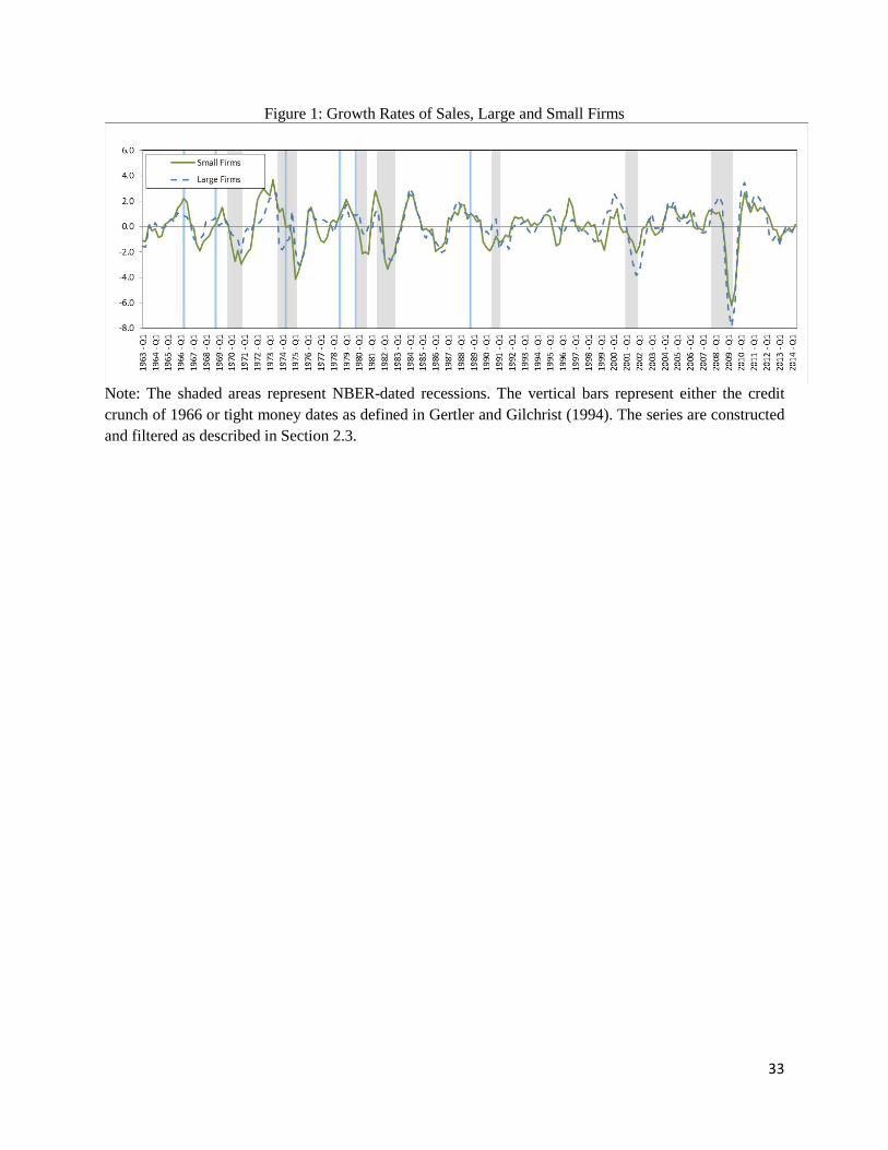
Figures 1-3 show the detrended constructed growth rate series. Figure 1 shows the series

of growth rates of sales for small and for large firms, starting from 1963.16 As can be seen from

the figure, around tight money dates prior to 1990, small firms' sales tend to drop more than the

large firms' sales as documented by Gertler and Gilchrist (1994). This also appears to be the case

around recessions prior to 1990. By contrast, in the three recessions of 1990-91, 2001, and 2007-

09 the opposite pattern is apparent: large firms' sales fall more following the beginning of the

recessions.

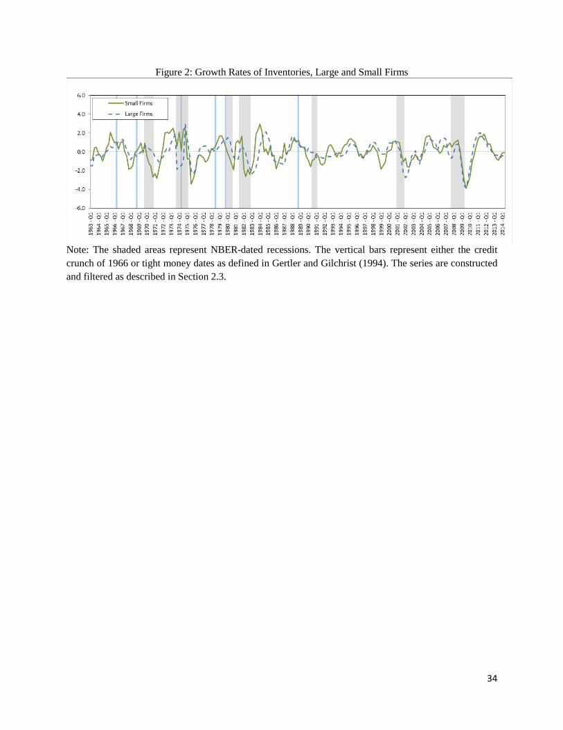
Figure 2 shows the series of growth rates of inventories. Focusing on recessions, we

observe that at the onset of recessions the growth rate of inventories follows a pattern similar to

the pattern of the growth rates of sales. In particular, in the recessions prior to 1990, the growth of

inventories of the small firms falls further than the growth of the large firms, whereas in the recent

three recessions, the inventories of the small firms do not fall more than the inventories of the large

firms.

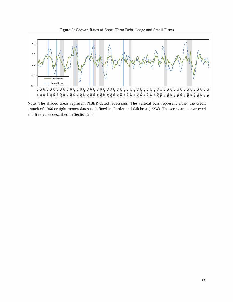
Figure 3 shows the series of growth of short-term debt. The short-term debt appears more

volatile for large firms than for small firms during the entire sample period. In particular, following

the tight money dates, the short-term debt of large firms grows more but then also falls to much

lower levels, after controlling for the trend. Around the tight money dates prior to 1990, there is

initially a large increase in the short-term debt of large firms followed by a sharp decline, while

the changes in short-term debt for small firms are much less pronounced. Following the 1988 and

1994 tight money dates, the growth rate of short-term debt of large firms is less volatile as

compared to the previous period. The large firms also show much more volatility in the growth

rate of short-term debt following recession peaks than do small firms; and this pattern holds for all

recessions in the sample.

The same picture emerges if we smooth the de-seasoned growth rates series with the

running medians instead of the Hodrick-Prescott filter. The figures suggest that around tight money

dates and at the onset of recessions, sales, inventories and short-term debt of small and large firms

behave differently. We thus proceed to quantify the responses.

16 Note that we apply the HP-filter to the series from Q1 1959 to Q2 2014.

14

4. Small and Large Firms around Tight Money Dates and the 2007-09 Episode

We now analyze the small and large firms’ responses around the tight money dates studied

by Gertler and Gilchrist (1994) and further extend the sample to additionally cover 1992-2014. We

then focus on the behavior of firms’ growth around the third quarter of 2008.

4.1. Tight Money Dates, 1960-2000

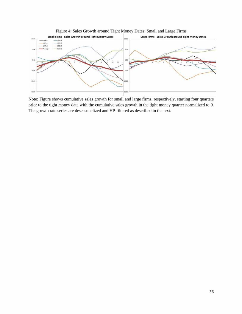
Figure 4 shows the behavior of the growth rates around each of the seven tight money date

episodes between 1960 and 2000 for small (Panel A) and for large (Panel B) firms, normalized to

0 at the calendar quarter of the tight money episode. Consistent with the earlier findings of Gertler

and Gilchrist (1994), following tight money dates, the sales of small firms fall more than the sales

of large firms.

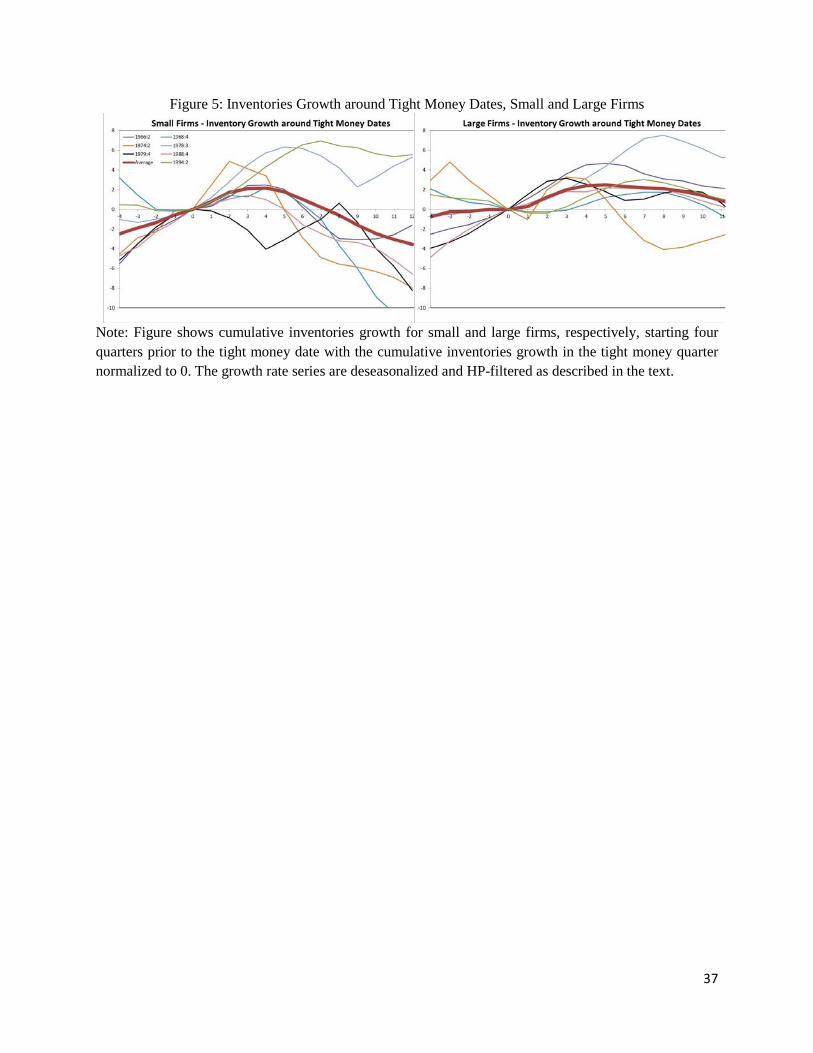
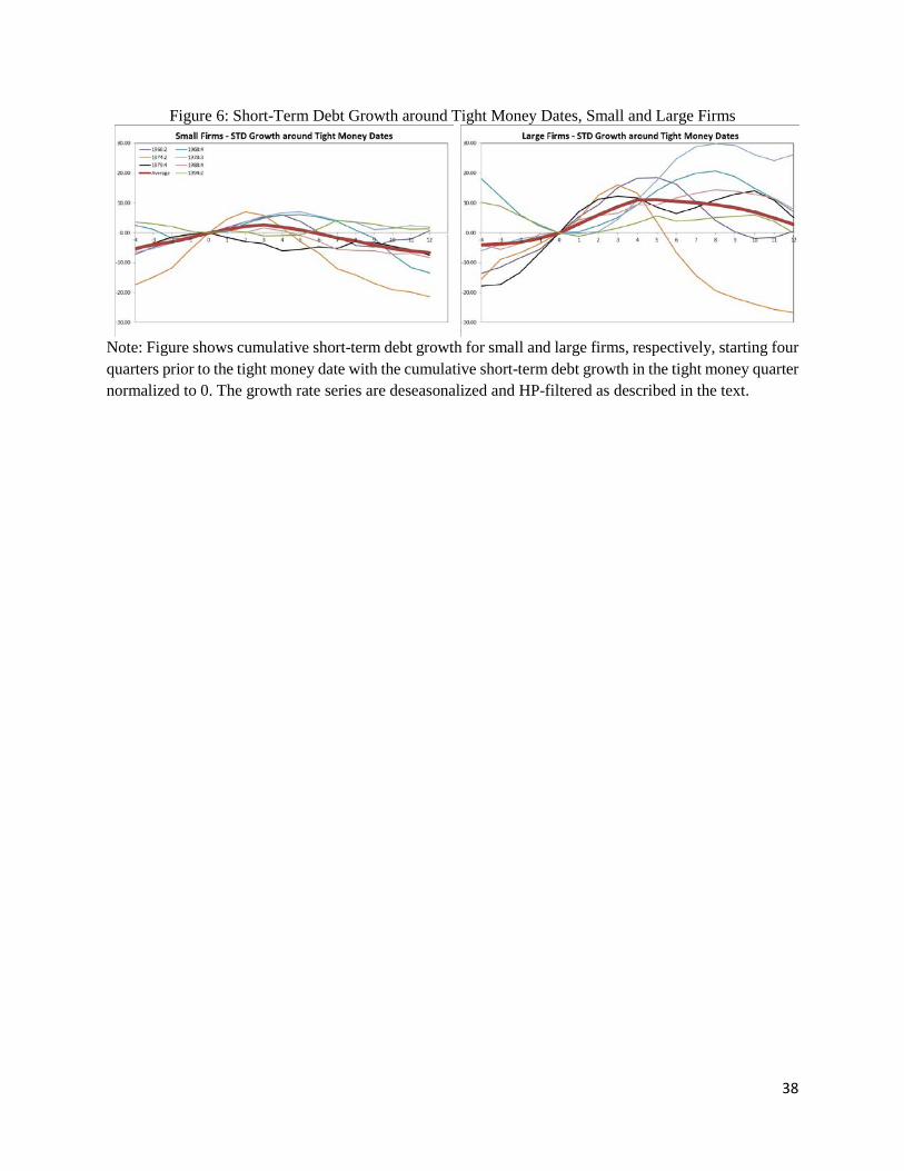
Figure 5 shows the behavior of the growth rates of inventories and Figure 6 shows the

behavior of the growth rates of short-term debt. The figures show that comparing from the tight

money date to the twelve quarters after the tight money date, the growth rate drops much more for

small firms than for large firms, as observed in Gertler and Gilchrist (1994). However, during these

twelve quarters following the time money dates, the peak of the large firm series reached after the

tight money date is often higher than the peak reached by the small firm series, especially for short-

term debt. In addition, for small firms, the growth rate reaches its peak at or soon after the tight

money date, and it falls below its tight money date value well before the end of the twelve-quarter

period. In contrast, for large firms, the growth rate reaches its peak, on average, a quarter after the

small firms’ peak and declines much slower, thereby not falling below its tight money date value

before the end of the twelve-quarter period. Consequently, the timing of the peaks and troughs in

the aftermath of the tight money dates is important for quantifying the differential growth rate

changes for small and large firms following tight money dates.

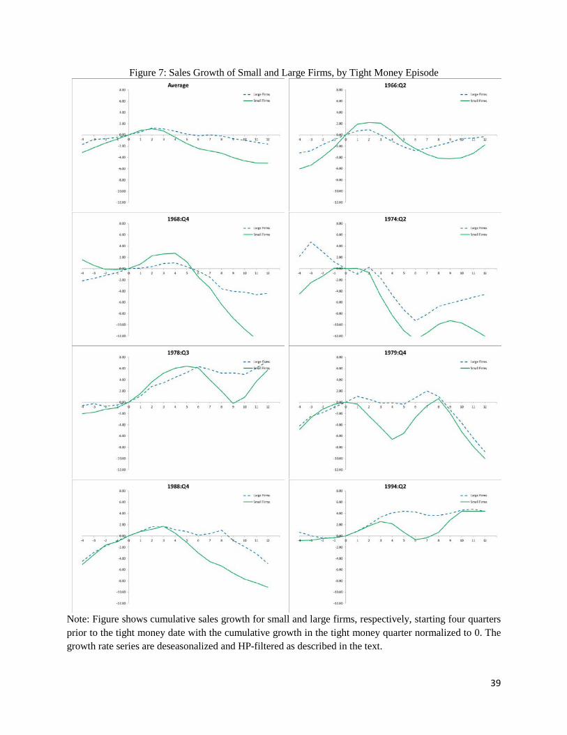
To further understand how the behavior of small versus large firms compares in each tight

money episode, Figures 7-9 plot, for each episode, the behavior of the series for small and large

firms on the same scale. The growth rates of sales of small and large firms exhibit very similar

behavior around each episode: the relative decline of the sales growth of small firms is much more

15

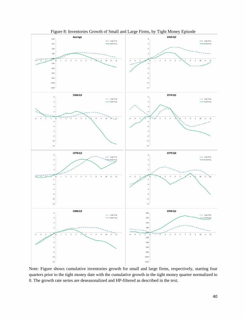
pronounced than the decline of the sales growth of large firms. The same holds for the growth rate

of inventories with the exception of the 1994 episode when the inventories of small firms kept

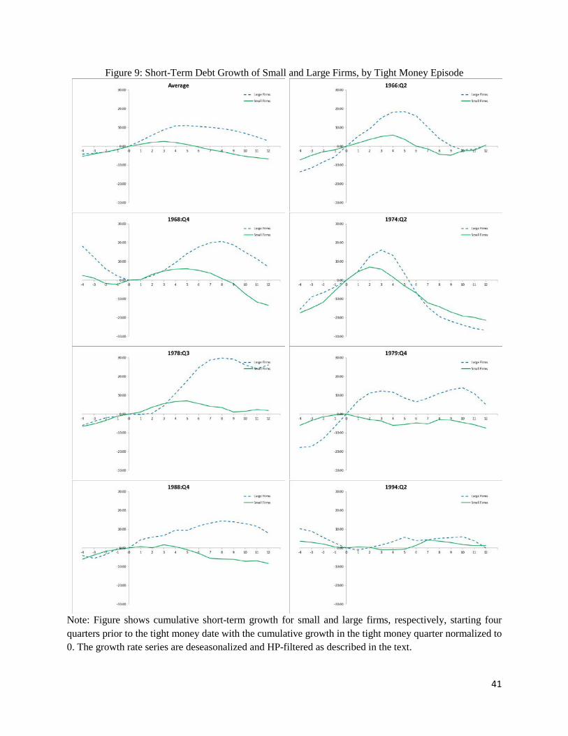
growing after the tight money date. As in Figure 6, the growth rate of the short-term debt of large

firms is more volatile than the growth rate of the short-term debt of small firms. The growth rate

of short-term debt for small firms is particularly less responsive to the tight money shocks in 1988

and 1994.

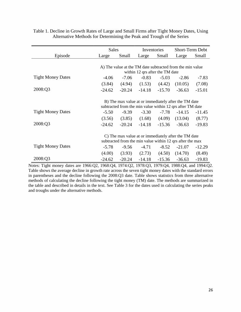
Finally, Table 1 contains the cumulative change in the growth rates of the series following

the tight money date, averaged across seven episodes of tight money dates: 1966:Q2, 1968:Q4,

1974:Q2, 1978:Q3, 1979:Q4, 1988:Q4, and 1994:Q2. Panel A shows the change of the growth rate

from the tight money date to the lowest value reached by the cumulative growth rate series within

the following 12 quarters after the date (which we refer to as "trough"), i.e., our first approach.

The growth rate of sales for small firms drops by 7.06 percent while the growth rate for large firms

drops by 4.06 percent. The growth rate of inventories for small firms drops by 5.03 percent, while

the growth rate for large firms drops by 0.83 percent. The growth rate of short-term debt for small

firms drops by 7.83 percent, while the growth rate for large firms drops by only 2.86 percent. These

results are consistent with Gertler and Gilchrist findings.

The sales, inventories, and short-term debt series, however, often keep growing past the

tight money date and reach their respective peaks a few quarters after the date before starting to

decline. The difference between the peaks reached by small and large firms is especially

pronounced for short-term debt growth (Figure 6), with large firms reaching a much higher peak

and a quarter later. Thus, calculating the change in the growth rate using the value at the tight

money date as the benchmark masks the differential dynamics of the small and large firms growth,

especially in short-term debt. We thus employ our second method of calculating the change in

growth rate following the tight money episode. We find the peak value of the series reached at or

a few quarters immediately after the tight money episode and subtract this value from the

subsequent trough reached within twelve quarters of the tight money date.

16

The results of this calculation are presented in Panel B of Table 1.17 As can be seen from

the table, under this approach to calculating the change in the growth rates, the growth rates of

sales and inventories of small firms still contract much more than those of large firms. However,

the short-term debt now shows a different picture. The growth rate of the short-term debt of large

firms declines 14.15 percent, while the growth rate of the small firms declines by 11.45 percent.

If the growth series reach their peaks a few quarters after the tight money date, it might

take longer than twelve quarters after the tight money date to reach their trough. To allow for the

possibility that the growth rate might not reach the trough within twelve quarters of the tight money

date, we employ our third approach to calculating the change in the growth rate whereby allowing

the trough value within up to twelve quarters after the peak is reached. The results of this

calculation are presented in Panel C of Table 1.18 As under the two approaches above, we find that

growth rates of sales and inventories of small firms contract more than the growth rates of sales

and inventories of large firms. As under the second approach above, we find that the growth rate

of the short-term debt of large firms declines more than the growth rate of small firms, 21.07

percent versus 12.29 percent.

4.2. The 2007-09 Episode

We now turn to the analysis of the behavior of sales, inventories and short-term debt in the

2008:Q3 episode. The collapse of Lehman Brothers Inc. in September 2008 and the ensuing

anguish over the possibility of government bailout sent financial markets to the verge of shutdown.

The description of the conditions on the credit markets following the third quarter of 2008 is similar

to the description of the conditions following the tight money dates. The period is widely

characterized as the period when credit became scarce and difficult to obtain (see, for example,

Wenzel, 2015). This raises a question of whether the relative behavior of small and large firms

around this date resembles the behavior during the earlier periods of tight money.

It is important to understand the events surrounding the date. December 2007 marks the

beginning of the deepest postwar recession. However, despite the brewing turmoil that had started

17 Table 3, Panel B shows the dates of the peaks of each series and the number of quarters to the subsequent trough used for calculations in Panel B of Table 1. 18 Table 3, Panel C shows the dates of the peaks of each series and the number of quarters to the subsequent trough used for calculations in Panel C of Table 2.

17

with the bailout of Bear Stearns, at the onset of the recession the signs of an economy-wide

downturn were mild and discussions about the beginning of the recession did not become prevalent

until the summer of 2008. Only toward the end of 2008, with the financial crisis in its full force,

did NBER announce that the recession had begun in December 2007.

Consequently, the analysis of the behavior of firms around the third quarter of 2008 can

also be seen as the analysis of the behavior at the onset of the 2007-09 recession. This can be easily

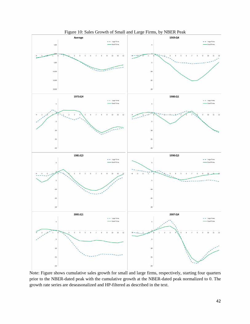
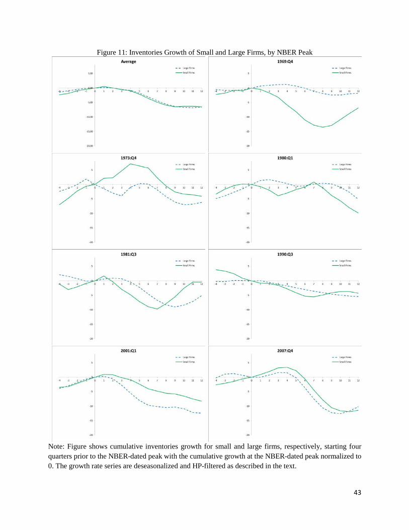
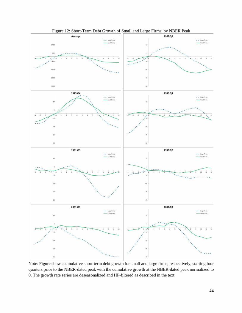
seen from the last panels of Figures 10-12 that show the behavior of the growth rates of sales,

inventories and short-term debt around the fourth quarter of 2007, the beginning of the 2007-09

recession. For both small and large firms sales do not stop growing until the third quarter of 2008

and inventories start falling only in the fourth quarter of 2008. Interestingly, large firms experience

a decline in the growth rate of short-term debt by the second quarter of 2008, while small firms'

debt only starts falling in the first quarter of 2009, i.e., almost a year later. Thus, the firms’ behavior

in the 2007-09 episode may be a response to tight money shocks, or adverse shocks that sent the

economy into a contraction at the end of 2007, or a combination of the two shocks.

Examining the last panels of Figures 10-12, we observe, first, that the sales of large firms

fall relatively more than the sales of small firms (Figure 10). Second, there is no substantial

difference in the relative behavior of the inventories of small and large firms (Figure 11). Finally,

third, the short-term debt of large firms falls relatively more than the short-term debt of small firms

(Figure 12).

Table 1 formalizes these observations by showing the change in the growth rate of the

series after the third quarter of 2008. As with the tight money dates episodes above, we employ

three different approaches to calculating the change. However, in contrast to the tight money

episodes studied in Section 4.1, all three approaches deliver quantitatively similar results (Table

1, Panels A-C). The results in the table show that the relative decline in the growth rates of sales

of large firms is larger than that of small firms, 24.62 percent and 20.24 percent, respectfully. The

growth rate of inventories for both large and small firms drops by a similar amount: by 14.18

percent for large firms and by 15.36 percent for small firms (Table 1, Panel B). The decline of the

growth rate short-term debt of large firms is much more pronounced than the decline for small

firms: the growth rate of short-term debt of large firms declines by 36.63 percent, while the growth

rate of small firms declines by 19.83 percent (Table 1, Panel B).

18

Consequently, the relative behavior of large versus small firms around the third quarter of

2008 differs from the behavior during the earlier episodes of tight money. In particular, while in

the pre-1990 episodes the sales of the small firms bear the effect of adverse shocks, in the 2007-

09 episode it is the sales of large firms that bear the effect and there is not much difference in the

inventory behavior. The results are particularly striking for short-term debt. We find that the short-

term debt contracts much more for large firms than for small firms. This observation holds around

the 2008:Q3 episode, and it also holds for the previous episodes of tight money if the calculation

of the change in the short-term debt of large firms takes into account a much longer period over

which the contraction for large firms takes place.

To the extent that the third quarter of 2008 can be characterized as a period of adverse

conditions in credit markets, the evidence points to large firms’ sales contracting more than small

firms’ following the tight money shock, which is in contrast to the prevailing view following

Gertler and Gilchrist (1994). This evidence, however, can also be characterized as evidence

describing the responses of firms to the shocks that cause recessions, which may or may not be

tight money shocks. To examine whether such behavior of small and large firms is specific to the

2007-09 recession, or is a characteristic of the earlier contractions, we proceed to examine the

relative behavior of the growth rates of sales, inventories, and short-term debt of small and large

firms at the onset of the postwar recessions.

5. Small and Large Firms around Recessions

In this section, we analyze the behavior of sales, inventories, and short-term debts around

the recession episodes. Figure 10 plots the growth rates of sales around NBER-dated peaks for

each episode. As can be seen from the figure, in the 1969 recession, the sales of small firms decline

substantially more than the sales of large firms. For the 1973, 1980, 1981, and 1990 recessions,

the figure does not provide a clear answer of whether large or small firms' sales experienced a

relatively larger decline. In these episodes, the series for small and large firms do not reach their

respective peaks simultaneously, and thus we return to this question below when we calculate the

changes between the peaks and troughs of the series.

19

In the 2001 recession, however, there is a clear difference between the growth rates of sales

of small and large firms. Both series remain negative for all twelve quarters following a recession

peak; however, large firms experience a much more drastic decline. Overall, while large firms'

sales appear to be more volatile at the start of the 2001 recession than in the earlier recessions, the

opposite is true for small firms' sales.

Figure 11 shows the growth rates of inventories around recessions. The inventories growth

of large firms also appears to be more responsive to the shocks at the onset of recession in the 2001

episode than in the earlier recessions. As in the case of sales, at the beginning of the 1969 recession

small firms' inventories decline substantially, while large firms' inventories do not start declining

until after a few quarters into the contraction with the subsequent decline being much smaller. This

picture is reversed for the 2001 recession: the inventories of large firms decline more than the

inventories of small firms. This reversal comes mostly from a substantial decline in the growth

rate of inventories of large firms at the onset of the 2001 recession as compared to the earlier

episodes.

Finally, Figure 12 shows the growth rate of short-term debt around recessions. The growth

rate of short-term debt of large firms in the pre-2000 recessions increases rapidly following the

start of a recession, and remains positive until almost the seventh quarter following the start. It

then declines rapidly, and remains negative through the 12th quarter following the peak. In the

2001 recession, the decline in short-term debt of large firms is almost immediate, falling negative

after the recession starts and continuing to decline through the following twelve quarters.

The short-term debt growth of small firms appears to become less responsive to the shocks

at the start of the 2001 recession and is less volatile than the growth rate of short-term debt of large

firms in the full sample period. In the earlier recessions, the short-term debt growth of small firms

increases modestly after the peak but turns negative after (on average) six quarters. In the 2001

recession, the short-term debt growth does turn negative in the fifth quarter after the peak but is

much flatter than in the earlier episodes. The figure reveals that in the 2001 recession, the short-

term debt of large firms declines substantially more than the short-term debt of small firms. With

the exception of the 2001 recession, the peaks of the series for small and large firms do not

coincide. As a result, the figure does not provide a clear answer about the relative magnitudes of

20

changes between small and large firms, and we proceed to calculate the changes between the peaks

and troughs.

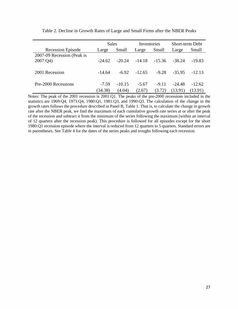
Table 2 shows the changes of the growth rates of sales, inventories, and short-term debt of

small and large firms between peaks and troughs. The examination of the figures above reveals

that the 2001 recession sales, inventories, and short-term debt of small and large firms show a

pattern that differs from the patterns observed in the earlier recession episodes. Thus, we group

the results for the five recessions prior to 2000 and present the results for the 2001 recession

separately. As the results in Row 2 (for the 2001 recession) and Row 3 (the average of the five

recessions prior to 2000) show, the behavior of small and large firms differs between the 2001

recession and the earlier recessions.

The behavior of sales, inventories, and short-term debt of small and large firms around the

starts of the five recessions (1969:Q4, 1973:Q4, 1980:Q1, 1981:Q3, and 1990:Q3) can be

summarized as follows. First, the growth rates of sales of small firms drop more than the growth

rate of sales of large firms: 10.15 percent and 7.59 percent, respectively. Second, the growth rate

of inventories of small firms also drops more (9.11 percent) than the growth rate of large firms

(5.67 percent). Finally, the growth rate of short-term debt of small firms drops less (12.62 percent)

than the growth rate of large firms (24.48 percent).

After the 2001 recession, the growth rates of all three series, sales, inventories, and short-

term debt, decline relatively more for large firms than for small firms (see Row 2 of Table 2). The

decline is particularly evident in sales and short-term debt. For example, the growth rate of short-

term debt of small firms declines by 12.13 percent while the growth of short-term debt of large

firms declines by 35.95 percent. Similarly, large firms experience a relatively large decline of sales

and short-term debt in the 2007-09 recession.

21

6. Discussion and Conclusions

We find that the main finding by Gertler and Gilchrist (1994) about the business cycle

fluctuations of sales, inventories, and short term debt for small and large firms can be reproduced

with our computations.19 Our analysis shows the following

1. The pattern of short-term debt growth is reversed, i.e., large firms' short-term debt

contracted relatively more than that of small firms, if we employ different methodologies

for determining the timing of peak and trough of the growth rate series around respective

tight money dates (Table 1, Panels B and C). Specifically, the alternative methodologies

take into account differential timing of when the series for large versus small firms reach

respective peaks and troughs following the tight money dates.

2. The evolution of sales, inventories, and short-term debt around the financial crisis of

2008:Q3 is the opposite of the behavior documented previously for previous tight money

dates. Specifically, the growth series for large firms contracted more than the growth series

for small firms following the episode. This finding is independent of the method used to

determine the timing of the changes around the episode (Table 1).

3. Finally, the pattern documented by Gertler and Gilchrist around tight money periods for

sales, inventories, and short term debt is the opposite of the pattern that we find for NBER

recessions, specifically, for short term debt and for the last two recessions (Table 2).

There are a few possible interpretations of our results. First, one might conjecture that the

distinction between small versus large is not a good approximation of the constrained versus not-

constrained dimension for firms via which the financial accelerator models work. To check on this

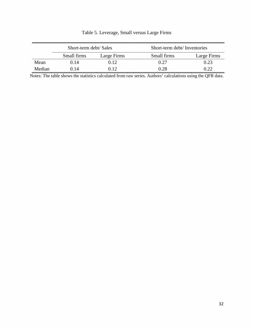
hypothesis, we compute two measures of leverage that can be constructed using the times series

in the study: (1) the ratio of short-term debt to sales, and (2) the ratio of short-term debt to

inventories. For most of the quarters in the entire sample period, small firms have higher leverage

than large firms. The median and mean for the times series of these ratios (see Table 5) confirm

that small firms are more leveraged, and thus likely more credit-constrained. Second, one might

conjecture that the small firms that we study are too large. To give some perspective, our small

19 Although we use a slightly smaller threshold for the definition of small firms - 25th percentile versus 30th percentile used by Gertler and Gilchrist (1994) – because it is not feasible to use the 30th percentile as cut off in the QFR data in 2014.

22

firms are firms that in 2014 had assets for less than 1 billion. This is a relatively large value. For

instance, about one third of the publicly traded firms are small by this measure. However, this

threshold is comparable and is even slightly smaller than the threshold for small firms used by

Gertler and Gilchrist. Studying smaller firms is feasible. However, smaller firms contribute a

smaller share of aggregate variables and thus have less impact on macro aggregates. With our

measure, by definition, small firms have 25 percent of the sales throughout the entire sample

period. Finally, it might be the case that the 2007-09 period was not a period of “tight money,”

i.e., a tightening of a financial or collateral constraint is not a good representation of the 2007-09

recession. Rather, the shock (or a combination of shocks) associated with the 2007-09 crisis (and

the recession) might primarily propagate via large firms. Although we favor the last possibility,

with the evidence at hand it is hard to rule out that our findings are due to a combination of these

reasons.

Our findings thus invite further research into the role of small versus large firms in

propagating the shocks during economic crisis. The behavior of firms during the 2007-09 episode

of worsening credit suggests that the economy does not entirely fit the longstanding model in

which small firms contract more than large firms in response to shocks. For example, one

possibility is that firms chose to deleverage in the aftermath of the 2007-09 crisis because they

receive news about slower future growth in productivity.

23

References

Abo-Zaid, Salem, and Anastasia S. Zervou. 2016. "Financing of Firms, Labor Reallocation and the Distributional Role of Monetary Policy," Texas A&M University, mimeo.

Adelino, Manuel, Song Ma and David Robinson. Forthcoming. “Firm Age, Investment Opportunities, and Job Creation”, Journal of Finance.

Barlevy, Gady. 2003. "Credit Market Frictions and the Allocation of Resources Over the Business Cycle," Journal of Monetary Economics, 50(8): 1795-1818.

Bernanke, Ben S., Gertler, Mark, and Gilchrist, Simon. 1996. "The Financial Accelerator and the Flight to Quality," The Review of Economics and Statistics, Vol. 78(1): 1-15.

Bernanke, Ben S., Gertler, Mark, and Gilchrist, Simon. 1999. "The Financial Accelerator in a Quantitative Business Cycle Framework," Handbook of Macroeconomics, in: J. B. Taylor & M. Woodford (ed.), Elsevier, Handbook of Macroeconomics, Ed. 1, Vol. 1, Chapter 21: 1341-1393.

Chari, V.V., Lawrence Christiano, and P. Kehoe. 2013. "The Gertler-Gilchrist Evidence on Small and Large Firm Sales," mimeo, Northwestern Univeristy. Accessed at http://faculty.wcas.northwestern.edu/~lchrist/research/cck/shell.pdf on July 1, 2015.

Coibon, Olivier. 2012. “Are the Effects of Monetary Policy Shocks Big or Small?” American Economic Journal: Macroeconomics, Vol. 4(2): 1-32.

Duygan-Bump, Burcu, Alex Levkov, and Judit Montoriol-Garriga. 2015. “Financing Constraints and Unemployment: Evidence from the Great Recession,” Journal of Monetary Economics, Vol. 75: 89–115.

Fort, Teresa C., John Haltiwanger, Ron S. Jarmin, and Javier Miranda. 2013. ”How Firms Respond to Business Cycles: The Role of Firm Age and Firm Size,” NBER Working Paper No. 19134.

Gertler, Mark, and Simon Gilchrist. 1994. "Monetary Policy, Business Cycles, and the Behavior of Small Manufacturing Firms," Quarterly Journal of Economics, 109(2): 309-340.

Gilchrist, Simon, Raphael Schoenle, Jae Sim, and Egon Zakrajsek. 2015. “Inflation Dynamics During the Financial Crisis,” Mimeo.

Gilchrist, Simon, and Egon Zakrajsek. 2012. "Credit Spreads and Business Cycle Fluctuations," American Economic Review, Vol. 102(4): 1692-1720.

Giroud, Xavier, and Holger M. Mueller. 2015. “Firm Leverage and Unemployment during the Great Recession,” NBER Working Paper No. 21076.

Foster, Lucia, Cheryl Grim, and John Haltiwanger. 2016. “Reallocation in the Great Recession: Cleansing or Not?” Journal of Labor Economics, Vol. 34(S1, Part 2): 293-331.

https://ideas.repec.org/a/tpr/restat/v78y1996i1p1-15.html

https://ideas.repec.org/a/tpr/restat/v78y1996i1p1-15.html

https://ideas.repec.org/s/tpr/restat.html

http://www.nber.org/people/xavier_giroud

http://www.nber.org/people/holger_mueller

http://www.nber.org/chapters/c13284

http://www.nber.org/chapters/c13284

24

Herrera, Ana Maria, Marek Kolar, and Raoul Minetti. 2011. “Credit Reallocation,” Journal of Monetary Economics, Vol. 58: 551-563.

Hetzel, Robert L. 2008. The Monetary Policy of the Federal Reserve: A History. Cambridge University Press, 380 pp..

Jermann, Urban, and Vincenzo Quadrini. 2006. "Financial Innovations and Macroeconomic Volatility," CEPR Discussion Papers 5727, C.E.P.R. Discussion Papers.

King, Wilford I. 1923. Employment Hours and Earnings in Prosperity and Depression, United States, 1920-1922. New York: National Bureau of Economic Research.

Kiyotaki, Nobuhiro, and John Moore. 1997. “Credit Cycles,” Journal of Political Economy, Vol. 105(2): 211-248.

Mehrotra, Neil, and Dmitriy Sergeyev. 2016. “Financial Shocks and Job Flows,” Bocconi University, Working Paper.

Moscarini, Giuseppe, and Fabien, Postel-Vinay. 2012. "The Contribution of Large and Small Employers to Job Creation in Times of High and Low Unemployment," American Economic Review, 102(6): 2509-2539.

Oliner, Steve, and Glenn D. Rudebusch. 1996a. “Is There a Broad Credit Channel for Monetary Policy?” Economic Review, Federal Reserve Bank of San Francisco, No. 1: 3-13.

Oliner, Steve, and Glenn D. Rudebusch. 1996b. “Monetary Policy and Credit Conditions: Evidence from the Composition of External Finance: Comment,” American Economic Review, Vol. 86, March: 300-309.

Romer, Christina D., and David H. Romer. 1990. "New Evidence on the Monetary Transmission Mechanism," Brookings Papers on Economic Activity, 1: 149-98.

Romer, Christina D., and David H. Romer. 1992. "Money Matters," mimeo, University of California Berkley.

Romer, Christina D., and David H. Romer. 2004. “A New Measure of Monetary Shocks: Derivation and Implications,” American Economic Review, Vol. 94(4): 1055-1084.

Romer, Christina D. 2010. "Back to a Better Normal: Unemployment and Growth in the Wake of the Great Recession," Remarks at the Woodrow Wilson School of Public and International Affairs, Princeton University, April 17.

Sahin, Aysegul, Sagiri Kitao, Anna Coroaton, and Sirgiu Laiu. 2011. "Why Small Businesses Were Hit Harder by the Recent Recession," Federal Reserve Bank of New York Current Issues in Economics and Finance, Volume 17, No. 4.

25

Siemer, Michael. 2014. “Firm Entry and Employment Dynamics in the Great Recession,” Finance and Economics Discussion Series, Federal Reserve Board, Working Paper 2014-56.

Smant, David. 2002. “Bank credit in the transmission of monetary policy: A critical review of the issues and evidence,” Working Paper, Erasmus University Rotterdam.

Tenreyro, Silvana, and Gregory Thwaites. Forthcoming. “Pushing on a String: US Monetary Policy is Less Powerful in Recessions,” American Economic Journal: Macroeconomics.

Wenzel, Robert. 2015. The Fed Flunks: My Speech at the New York Federal Reserve Bank. Lulu Publishing. 74 pages.

http://personal.lse.ac.uk/tenreyro/TandT.pdf

http://personal.lse.ac.uk/tenreyro/TandT.pdf

26

Table 1. Decline in Growth Rates of Large and Small Firms after Tight Money Dates, Using Alternative Methods for Determining the Peak and Trough of the Series

Episode Sales Inventories Short-Term Debt

Large Small Large Small Large Small

A) The value at the TM date subtracted from the min value within 12 qrs after the TM date

Tight Money Dates -4.06 -7.06 -0.83 -5.03 -2.86 -7.83 (3.84) (4.94) (1.53) (4.42) (10.05) (7.08)

2008:Q3 -24.62 -20.24 -14.18 -15.70 -36.63 -15.01 B) The max value at or immediately after the TM date

subtracted from the min value within 12 qrs after TM date Tight Money Dates -5.50 -9.39 -3.30 -7.78 -14.15 -11.45

(3.56) (3.85) (1.68) (4.09) (13.04) (8.77) 2008:Q3 -24.62 -20.24 -14.18 -15.36 -36.63 -19.83 C) The max value at or immediately after the TM date

subtracted from the min value within 12 qrs after the max Tight Money Dates -5.78 -9.56 -4.71 -8.52 -21.07 -12.29 (4.00) (3.93) (2.73) (4.50) (14.70) (8.49) 2008:Q3 -24.62 -20.24 -14.18 -15.36 -36.63 -19.83

Notes: Tight money dates are 1966:Q2, 1968:Q4, 1974:Q2, 1978:Q3, 1979:Q4, 1988:Q4, and 1994:Q2. Table shows the average decline in growth rate across the seven tight money dates with the standard errors in parentheses and the decline following the 2008:Q3 date. Table shows statistics from three alternative methods of calculating the decline following the tight money (TM) date. The methods are summarized in the table and described in details in the text. See Table 3 for the dates used in calculating the series peaks and troughs under the alternative methods.

27

Table 2. Decline in Growth Rates of Large and Small Firms after the NBER Peaks

Recession Episode Sales Inventories Short-term Debt

Large Small Large Small Large Small 2007-09 Recession (Peak is 2007:Q4) -24.62 -20.24 -14.18 -15.36 -38.24 -19.83 2001 Recession -14.64 -6.92 -12.65 -9.28 -35.95 -12.13 Pre-2000 Recessions -7.59 -10.15 -5.67 -9.11 -24.48 -12.62 (34.38) (4.04) (2.67) (3.72) (13.91) (13.91)

Notes: The peak of the 2001 recession is 2001:Q1. The peaks of the pre-2000 recessions included in the statistics are 1969:Q4, 1973:Q4, 1980:Q1, 1981:Q3, and 1990:Q3. The calculation of the change in the growth rates follows the procedure described in Panel B, Table 1. That is, to calculate the change in growth rate after the NBER peak, we find the maximum of each cumulative growth rate series at or after the peak of the recession and subtract it from the minimum of the series following the maximum (within an interval of 12 quarters after the recession peak). This procedure is followed for all episodes except for the short 1980:Q1 recession episode where the interval is reduced from 12 quarters to 5 quarters. Standard errors are in parentheses. See Table 4 for the dates of the series peaks and troughs following each recession.

28

Table 3. Dating of the Peaks and Troughs of the Cumulative Growth Rate Series after Tight Money Dates

A) Peak is defined by the value at the TM date. Trough is defined by the min value within 12

quarters after the TM date

Tight Money Dates Episodes

Small Firms Large Firms Sales Inventory STD Sales Inventory STD

2008:Q3 Episode Peak 2008:Q3 2008:Q3 2008:Q3 2008:Q3 2008:Q3 2008:Q3

No of qrs to Trough 5 5 8 7 8 8 1994:Q2 Episode Peak 1994:Q2 1994:Q2 1994:Q2 1994:Q2 1994:Q2 1994:Q2







No of qrs to Trough 9 6 9 1 9 10

29

B) Peak is defined by the max value at or immediately after the TM date, and trough is defined by the min value within 12 quarters after TM date












30

C) Peak is defined by the max value at or immediately after the TM date, and trough is defined by the min value within 12 quarters after the peak












31

Table 4. Peaks and Troughs of the Cumulative Growth Rate Series around NBER Recessions

NBER Peaks Small Firms Large Firms

Sales Inventory STD Sales Inventory STD

2007:Q4 Peak 2008:Q3 2008:Q3 2008:Q4 2008:Q3 2009:Q1 2008:Q2 No of qrs to Trough 5 5 7 7 6 9







Notes: The table shows (1) peaks - the date at or after the peak of the recession when the respective cumulative growth rate series achieve their local maximum, and (2) troughs – the date at or after the peak of the recession when the respective cumulative growth rate series achieves their local minimum following the maximum (within an interval of 12 quarters after the peak). This procedure is followed for all recession episodes except for the short 1980:Q1 episode where the interval is reduced from 12 quarters to 5 quarters.

32

Table 5. Leverage, Small versus Large Firms

Short-term debt/ Sales Short-term debt/ Inventories Small firms Large Firms Small firms Large Firms Mean 0.14 0.12 0.27 0.23 Median 0.14 0.12 0.28 0.22

Notes: The table shows the statistics calculated from raw series. Authors’ calculations using the QFR data.

33

Figure 1: Growth Rates of Sales, Large and Small Firms

Note: The shaded areas represent NBER-dated recessions. The vertical bars represent either the credit crunch of 1966 or tight money dates as defined in Gertler and Gilchrist (1994). The series are constructed and filtered as described in Section 2.3.

34

Figure 2: Growth Rates of Inventories, Large and Small Firms


35

Figure 3: Growth Rates of Short-Term Debt, Large and Small Firms


36

Figure 4: Sales Growth around Tight Money Dates, Small and Large Firms

Note: Figure shows cumulative sales growth for small and large firms, respectively, starting four quarters prior to the tight money date with the cumulative sales growth in the tight money quarter normalized to 0. The growth rate series are deseasonalized and HP-filtered as described in the text.

37

Figure 5: Inventories Growth around Tight Money Dates, Small and Large Firms

Note: Figure shows cumulative inventories growth for small and large firms, respectively, starting four quarters prior to the tight money date with the cumulative inventories growth in the tight money quarter normalized to 0. The growth rate series are deseasonalized and HP-filtered as described in the text.

38

Figure 6: Short-Term Debt Growth around Tight Money Dates, Small and Large Firms

Note: Figure shows cumulative short-term debt growth for small and large firms, respectively, starting four quarters prior to the tight money date with the cumulative short-term debt growth in the tight money quarter normalized to 0. The growth rate series are deseasonalized and HP-filtered as described in the text.

39

Figure 7: Sales Growth of Small and Large Firms, by Tight Money Episode

Note: Figure shows cumulative sales growth for small and large firms, respectively, starting four quarters prior to the tight money date with the cumulative growth in the tight money quarter normalized to 0. The growth rate series are deseasonalized and HP-filtered as described in the text.

40

Figure 8: Inventories Growth of Small and Large Firms, by Tight Money Episode

Note: Figure shows cumulative inventories growth for small and large firms, respectively, starting four quarters prior to the tight money date with the cumulative growth in the tight money quarter normalized to 0. The growth rate series are deseasonalized and HP-filtered as described in the text.

41

Figure 9: Short-Term Debt Growth of Small and Large Firms, by Tight Money Episode

Note: Figure shows cumulative short-term growth for small and large firms, respectively, starting four quarters prior to the tight money date with the cumulative growth in the tight money quarter normalized to 0. The growth rate series are deseasonalized and HP-filtered as described in the text.

42

Figure 10: Sales Growth of Small and Large Firms, by NBER Peak

Note: Figure shows cumulative sales growth for small and large firms, respectively, starting four quarters prior to the NBER-dated peak with the cumulative growth at the NBER-dated peak normalized to 0. The growth rate series are deseasonalized and HP-filtered as described in the text.

43

Figure 11: Inventories Growth of Small and Large Firms, by NBER Peak

Note: Figure shows cumulative inventories growth for small and large firms, respectively, starting four quarters prior to the NBER-dated peak with the cumulative growth at the NBER-dated peak normalized to 0. The growth rate series are deseasonalized and HP-filtered as described in the text.

44

Figure 12: Short-Term Debt Growth of Small and Large Firms, by NBER Peak

Note: Figure shows cumulative short-term debt growth for small and large firms, respectively, starting four quarters prior to the NBER-dated peak with the cumulative growth at the NBER-dated peak normalized to 0. The growth rate series are deseasonalized and HP-filtered as described in the text.

Documents

Revisiting Gertler-Gilchrist Evidence on the Behavior of Small and