REVISED ANALYSIS OF ORIFICE METER EXPANSION FACTOR · PDF fileREVISED ANALYSIS OF ORIFICE METER EXPANSION FACTOR DATA ... the effect of an assumption made during data reduction. In

Catalog No. L52299

REVISED ANALYSIS OF ORIFICE METER EXPANSION FACTOR DATA

PR-015-08602

Prepared for the Measurement Technical Committee

of Pipeline Research Council International, Inc.

Prepared by: SOUTHWEST RESEARCH INSTITUTE

Mechanical and Materials Engineering Division 6220 Culebra Road

San Antonio, TX USA 78238-5166

Authors D.L. George, Ph.D.

Publication Date: October 15, 2008

This report is furnished to Pipeline Research Council International, Inc. (PRCI) under the terms of SwRI® Contract 18.14326, between PRCI and Southwest Research Institute. The contents of this report are published as received from Southwest Research Institute. The opinions, findings, and conclusions expressed in the report are those of the authors and not necessarily those of PRCI, its member companies, or their representatives. Publication and dissemination of this report by PRCI should not be considered an endorsement by PRCI or Southwest Research Institute, or the accuracy or validity of any opinions, findings, or conclusions expressed herein. In publishing this report, PRCI makes no warranty or representation, expressed or implied, with respect to the accuracy, completeness, usefulness, or fitness for purpose of the information contained herein, or that the use of any information, method, process, or apparatus disclosed in this report may not infringe on privately owned rights. PRCI assumes no liability with respect to the use of, or for damages resulting from the use of, any information, method, process, or apparatus disclosed in this report. The text of this publication, or any part thereof, may not be reproduced or transmitted in any form by any means, electronic or mechanical, including photocopying, recording, storage in an information retrieval system, or otherwise, without the prior, written approval of PRCI.

Pipeline Research Council International Catalog No. L52299

Copyright 2008 All Rights Reserved by Pipeline Research Council International, Inc.

PRCI Reports are published by Technical Toolboxes, Inc.

3801 Kirby Drive, Suite 340 Houston, Texas 77098 Tel: 713-630-0505 Fax: 713-630-0560 Email: [email protected]

iii

REVISED ANALYSIS OF ORIFICE METER EXPANSION FACTOR DATA

D. L. George, Ph.D.

SOUTHWEST RESEARCH INSTITUTE®

Mechanical and Materials Engineering Division 6220 Culebra Road

San Antonio, Texas, USA 78238–5166

ABSTRACT Orifice meter expansion factor data collected at Southwest Research Institute (SwRI) between 2003 and 2005 have been reviewed to assess the effect of an assumption made during data reduction. In accordance with the North American orifice meter standard, AGA Report No. 3, Part 1, the data were originally analyzed using a constant value of the isentropic exponent, k = 1.3. By comparison, the expansion factor equation adopted by ISO employs the real isentropic exponent, κ, which is a function of pressure, temperature, and gas composition.

The SwRI orifice meter expansion factor data have been re-reduced, using values of the real isentropic exponent, κ, from archived test data in place of the ideal gas value of k = 1.3. The original expansion factor data were obtained in such a way that the expansion factor values themselves were unaffected by the value of the isentropic exponent. However, the use of k = 1.3 influenced the values of the acoustic ratio, the independent variable used with the AGA and ISO equations to compute values of the expansion factor in measurement applications. The use of the ideal isentropic exponent in the original SwRI data, instead of real values of the isentropic exponent, was found to have caused an average shift in the acoustic ratio of +0.13%. The original SwRI expansion factor data and the revised data were graphed together, and the differences between the original and revised data sets were judged to be negligible. Both data sets were also compared to expansion factor curves obtained using the Buckingham equation of the AGA standard and the ISO 5167-2:2003 equation. The original assessment of the agreement between the SwRI data and the two correlations was found to still be valid. Both the original and revised SwRI expansion factor data are now available to the natural gas industry, to assist in further investigations of the orifice meter expansion factor.

iv

EXECUTIVE SUMMARY Until recently, the expansion factor Y1 used to account for the expansibility of gases relative to liquids in orifice meters was calculated from the Buckingham equation. This equation was adopted for both the North American orifice meter standard, AGA Report No. 3, Part 1, and the international standard, ISO 5167. In light of new data collected in the U.S. and Europe since the early 1980s, ISO adopted a new expansion factor equation in 2003, which disagrees with the AGA equation under some low-pressure, high-flow conditions.

To help resolve this disagreement, research at Southwest Research Institute (SwRI) in 2004 obtained additional experimental data to determine orifice meter expansion factors. Tests were performed in the SwRI Metering Research Facility (MRF) for a range of β ratios between 0.25 and 0.75, in 3-inch, 4-inch, and 6-inch line diameters. The results were eventually used in support of a decision to revise the expansion factor equation in the North American orifice meter standard. In those studies, a constant value of the isentropic exponent, k = 1.3, was used instead of the real compressible fluid isentropic exponent, κ, which is a function of pressure, temperature, and gas composition. This approach is accepted practice in accord with AGA Report No. 3, Part 1. However, the ISO expansion factor formula requires the use of the real isentropic exponent.

The orifice meter expansion factor data collected at SwRI have now been re-reduced, using the real isentropic exponent, κ, in place of the approximate ideal gas value of k = 1.3. For this, values of the real isentropic exponents for the natural gas test streams were retrieved from the MRF data archives. Values of κ computed for the recorded flowing conditions and gas compositions, using the more recent AGA-10 equation of state, agreed with the original archived values computed using AGA-8 to within the stated uncertainty of ±0.1% of both equations. Therefore, the original archived values of κ were used to re-reduce the data.

The original SwRI data were obtained through a procedure such that the derived expansion factor values were unaffected by the values used for the isentropic exponent. Similarly, the calibrations of the critical flow nozzles used to obtain the reference flow rates are independent of the isentropic exponent. Because of this, the expansion factor values themselves were unaffected by the assumption of k = 1.3. Instead, the use of a constant isentropic exponent influenced the values of the acoustic ratio, ΔP/κP1, the independent variable used with the Buckingham and ISO correlations to compute values of the expansion factor in measurement applications.

The use of the ideal isentropic exponent instead of real values of κ in the original SwRI data caused shifts in the acoustic ratio ranging from -0.09% to +0.45%, with an average shift of +0.13%. Shifts larger than +0.25% were commonly seen in cases where the line pressure exceeded 115 psia and ΔP/κP1 was less than 0.018. The original SwRI expansion factor data were plotted versus both ΔP/kP1 (using the ideal isentropic exponent of 1.3) and ΔP/κP1 (using the real isentropic exponents), and the differences between the original and revised data sets were found to be negligible. Both data sets were also compared to expansion factor curves obtained using the Buckingham equation and the ISO 5167-2:2003 equation. The original assessment of the agreement between the data and the two correlations was found to still be valid. Both the original and revised SwRI expansion factor data are available in electronic format, so that they may be used by the natural gas industry for comparison to the revised expansion factor equation in AGA-3, Part 1, and in other investigations of the orifice meter expansion factor.

v

TABLE OF CONTENTS Page

1. INTRODUCTION ........................................................................................................................... 1 1.1 BACKGROUND..................................................................................................................... 1 1.2 ORIGINAL SWRI EXPERIMENTAL DATA ............................................................................. 2 1.3 SCOPE OF WORK AND TECHNICAL APPROACH ................................................................... 2

2. REVIEW AND REPROCESSING OF EXPANSION FACTOR DATA ....................................... 4 2.1 EXPANSION FACTOR FORMULAS ........................................................................................ 4 2.2 DERIVATION OF EXPANSION FACTORS FROM SWRI DATA................................................. 4 2.3 LIMITED DEPENDENCE OF SWRI DATA ON ISENTROPIC EXPONENT DATA ........................ 5 2.4 ANALYSIS USING REAL ISENTROPIC EXPONENTS .............................................................. 6

2.4.1 Comparison of Isentropic Exponents Computed by AGA-8 and AGA-10.............. 6 2.4.2 Use of Archived Spreadsheet Data ........................................................................ 6

2.5 COMPARISON OF RESULTS .................................................................................................. 7 3. CONCLUSIONS ........................................................................................................................... 11 REFERENCES ........................................................................................................................................... 12 APPENDIX A: REVISED EXPANSION FACTOR DATA, 3-INCH ORIFICE METER TUBE ............ 13 APPENDIX B: REVISED EXPANSION FACTOR DATA, 4-INCH ORIFICE METER TUBE ............ 19 APPENDIX C: REVISED EXPANSION FACTOR DATA, 6-INCH ORIFICE METER TUBE ............ 31

vi

LIST OF FIGURES Page FIGURE 2-1. EXAMPLE OF A CORRELATION USED TO OBTAIN EXPANSION FACTOR

VALUES FROM THE SWRI EXPERIMENTAL DATA (MORROW, 2004)...................................5 FIGURE 2-2. COMPARISON OF DATA FROM THE 4-INCH METER TUBE, β = 0.50,

PRESSURE TAP #1, USING BOTH K = 1.3 AND ACTUAL VALUES OF κ, TO THE BUCKINGHAM CORRELATION. ....................................................................................9

FIGURE 2-3. COMPARISON OF DATA FROM THE 4-INCH METER TUBE, β = 0.50, PRESSURE TAP #1, USING BOTH K = 1.3 AND ACTUAL VALUES OF κ, TO THE ISO CORRELATION. .....................................................................................................9

FIGURE 2-4. COMPARISON OF DATA FROM THE 6-INCH METER TUBE, β = 0.35, PRESSURE TAP #2, USING BOTH K = 1.3 AND ACTUAL VALUES OF κ, TO THE BUCKINGHAM CORRELATION. ..................................................................................10

FIGURE 2-5. COMPARISON OF DATA FROM THE 6-INCH METER TUBE, β = 0.35, PRESSURE TAP #2, USING BOTH K = 1.3 AND ACTUAL VALUES OF κ, TO THE ISO CORRELATION. ...................................................................................................10

LIST OF TABLES Page TABLE 2-1. RANGES OF REAL VALUES OF ISENTROPIC EXPONENTS DURING THE 2004

EXPANSION FACTOR TESTS AT SWRI. ................................................................................8 TABLE 2-2. SHIFTS IN THE AVERAGE ACOUSTIC RATIO, ΔP/(κP1), DUE TO THE USE OF

A CONSTANT VALUE OF K = 1.3 IN CALCULATIONS. ...........................................................8

vii

This page is intentionally blank.

viii

ACKNOWLEDGMENTS The author would like to thank several individuals for their help with this project. Foremost is Tom Morrow, who was extensively involved in the revision and publication of the Third Edition of API MPMS Chapter 14.1. Dr. Morrow’s insight on his previous expansion factor studies is greatly appreciated. The author would also like to thank two SwRI staff members for their help: Sarah Treadwell, who compared equation-of-state calculations by AGA-8 and AGA-10 and assisted in uncertainty evaluations, and Leonard Morgan, who re-reduced the original data for use in this report.

1

1. INTRODUCTION 1.1 BACKGROUND As noted by Morrow (2004), the equation for the mass flow rate of a liquid or gas through an orifice meter takes the following form:

( )2112

1 24

PPgdYECq cvdm −= ρπ (1)

Here, qm = mass flow rate

Cd = orifice meter discharge coefficient

Ev = velocity of approach factor

Y1 = expansion factor

d = orifice bore diameter

gc = gravitational constant

ρ1 = gas density upstream of the orifice plate

P1 = static pressure upstream of the orifice plate

P2 = static pressure downstream of the orifice plate

ΔP = P1 – P2 = pressure difference across the orifice plate.

By convention, the orifice meter discharge coefficient, Cd, is the same in gas flows as in liquid flows for the same value of Reynolds number and orifice meter diameter ratio (β ratio). However, gases and liquids expand differently downstream of an orifice plate, and these differences can affect the pressure differential across the orifice. The differences are accounted for by the expansion factor, Y1. The expansion factor is an empirical correction factor, the ratio of the discharge coefficient in a compressible flow to the discharge coefficient in an incompressible flow under the same conditions. For incompressible liquids, the value of the expansion factor, Y1, is 1.0 by definition. For gases, the expansion factor is generally non-zero, and is calculated empirically as a function of β, the ratio of the orifice bore diameter to the meter tube diameter; the ratio of the pressure differential across the orifice plate to the upstream static pressure (ΔP/P1); and the ideal isentropic exponent of the gas, k.

Typically, the expansion factor is calculated from the Buckingham equation (Buckingham, 1932). This equation was adopted for both the North American orifice meter standard, AGA Report No. 3, Part 1 (American Gas Association, 2003) (also known as API Manual of Petroleum Measurement Standards Chapter 14.3, Part 1), and the international ISO 5167 standard (ISO, 1991). Since 1986, questions have been raised concerning the accuracy of the Buckingham equation, in the light of new data collected in the U.S. and Europe. In 2003, ISO adopted a new expansion factor equation (Reader-Harris, 1998) based on orifice coefficient data

2

taken since the early 1980s. This formula disagrees with the AGA equation under certain low-pressure, high-flow conditions.

In light of this disagreement, several organizations in the U.S. natural gas industry requested an exploratory project to acquire additional orifice meter expansion factor data in natural gas. It was anticipated that additional expansion factor data could guide a decision by the U.S. natural gas industry to (1) adopt the new ISO expansion factor equation, (2) reaffirm the Buckingham equation, or (3) to develop a new expansion factor equation altogether.

1.2 ORIGINAL SWRI EXPERIMENTAL DATA From 2003 to 2005, Gas Technology Institute (GTI), API, and Gas Processors Association (GPA) funded research at Southwest Research Institute (SwRI) to experimentally determine orifice meter expansion factors. Tests were performed in the SwRI Metering Research Facility (MRF) for a range of β ratios between 0.25 and 0.75, in 3-inch, 4-inch, and 6-inch line diameters. The results of these studies (Morrow, 2004 and 2005) were eventually used in support of a decision to revise the expansion factor equation in the North American orifice meter standard and produce a new equation for Y1.

In the SwRI studies, a constant value of the isentropic exponent, k = 1.3, was used instead of the real compressible fluid isentropic exponent, κ, which is a function of pressure, temperature, and gas composition. This approach is accepted practice in accord with AGA Report No. 3, Part 1. By comparison, the expansion factor equation adopted by ISO employs only the real isentropic exponent. The objective of the work reported here is to revise the expansion factor data collected at SwRI between 2003 and 2005, using values of the real isentropic exponents computed from data gathered during the tests. The analyzed data are compared to the original data reduced using the constant, ideal isentropic exponent; to the Buckingham expansion factor equation; and to the ISO 5167-2:2003 equation (ISO, 2003). The revised expansion factor data and the comparisons in this report are provided to the natural gas industry to help in any further review of the expansion factor equations. 1.3 SCOPE OF WORK AND TECHNICAL APPROACH The work to produce new expansion factor data proceeded in two steps. In the first step, temperature, pressure, and gas composition data recorded during the MRF expansion factor tests between 2003 and 2005 were retrieved from the MRF data archives. The archived data files also included values of the real isentropic exponent for each test run, computed using the AGA-8 equation of state (American Gas Association, 1994) and the gas composition data. The original spreadsheets used to calculate new values of the expansion factor were also retrieved from the MRF archives. Using this information, the data were analyzed again using the real values of the isentropic exponent. In the second step, four sets of data were graphed for comparison to one another:

• Original SwRI expansion factor data derived using the constant isentropic exponent of k = 1.3.

3

• Revised SwRI expansion factor data derived using the real isentropic exponents.

• Expansion factor curves obtained using the Buckingham equation.

• Expansion factor curves obtained using the ISO 5167-2:2003 equation. This report compares the original and revised SwRI expansion factor values, and the expansion factors generated by the two correlative formulas of Buckingham and ISO 5167. The report also discusses the impact of using real versus constant isentropic exponents in the correlation for Y1. Both the original and revised data are available in electronic form; graphical comparisons of both sets of data to the correlations appear in appendices to this report.

4

2. REVIEW AND REPROCESSING OF EXPANSION FACTOR DATA 2.1 EXPANSION FACTOR FORMULAS For many years, the Buckingham correlation (Buckingham, 1932) for the expansion factor in a flange-tap orifice meter was recommended by both AGA Report No. 3 and ISO 5167 for the measurement of natural gas. The Buckingham equation takes the form of Equation 2.

( )1

41 34.041.01

kPPY Δ

+−= β (2)

Expansion factor data published in the 1980s and later were found to be higher than values predicted by Equation 2, which led Reader-Harris (1998) to use the more recent data to develop a new correlation for the expansion factor, shown here as Equation 3.

( )⎥⎥

⎦

⎤

⎢⎢

⎣

⎡⎟⎟⎠

⎞⎜⎜⎝

⎛−++−=

κ

ββ1

1

2841 193.0256.0351.01

PPY (3)

Here, κ indicates the real isentropic exponent of the gas, as opposed to the ideal isentropic exponent, k, obtained by assuming ideal gas behavior. In 2003, the Reader-Harris correlation was recommended in ISO 5167-2 for computing orifice meter expansion factors. Morrow (2004) discusses the data used to generate both correlations, the disagreements between the data and the Buckingham correlation, and the questions raised concerning the soundness of the Reader-Harris correlation. 2.2 DERIVATION OF EXPANSION FACTORS FROM SWRI DATA As discussed by Morrow (2004), experiments to obtain expansion factors in compressible flows require a given orifice plate to be tested at a constant Reynolds number for different values of the acoustic ratio, ΔP/(kP1). This can be illustrated by rearranging Equation 1 as follows:

( )211

21

24

PPgdE

qYCcv

md

−=

ρπ (4)

Here, the right hand side of the equation contains quantities that can be measured directly, without knowledge of the Reynolds number at the orifice meter. In the case of the test loops at SwRI, the mass flow rate, qm, is determined using traceable weigh tank calibrations of critical flow nozzles, and temperature and pressure measurements at the nozzles. The velocity of approach factor, Ev, and the bore diameter, d, depend only on the orifice plate geometry; gc is a physical constant; the gas density, ρ1, is determined from direct measurements of temperature, pressure, and gas composition, and from the AGA-8 equation of state; and the static pressures P1 and P2 are determined using pressure transmitters. The product on the left-hand side of Equation 4, CdY1, is obtained from the measured quantities on the right-hand side of the equation. The SwRI expansion factor data were obtained by performing a linear regression of CdY1 versus the ratio of ΔP/P1, and then determining the intercept of the best-fit line, as illustrated in Figure 2-1. As ΔP approaches zero, the flow approaches the condition of incompressibility; the expansion factor approaches 1; and the

5

product of CdY1 approaches the value of the discharge coefficient in incompressible flow, Cd. Dividing experimental values of CdY1 by the intercept, Cd, produced the values of the expansion factor, Y1. As Morrow noted, if the Reynolds number was to change systematically during a test, the resulting change in the discharge coefficient would be incorrectly interpreted as an expansion factor effect. Random variations in Reynolds number will increase the scatter, particularly at low values of ΔP/P1, but do not invalidate the test results.

ΔP/P1

0.00 0.05 0.10 0.15 0.20

Cd*

Y 1

0.565

0.570

0.575

0.580

0.585

0.590

0.595

0.600

0.605

0.610

Dm = 4.028-inch, β = 0.50, 01/26/2004Linear regression curve fit

Pressure tap #1Intercept: Cd*Y1 = 0.606028Slope: -0.185951

Figure 2-1. Example of a correlation used to obtain expansion factor values from the

SwRI experimental data (Morrow, 2004).

2.3 LIMITED DEPENDENCE OF SWRI DATA ON ISENTROPIC EXPONENT DATA Equation 4 also demonstrates the limited extent to which the assumption of an isentropic exponent of k = 1.3 affects the SwRI data. The mass flow rate, qm, is determined using traceable weigh tank calibrations of critical flow nozzles, and temperature and pressure measurements at the nozzles. The nozzle calibration curves are self-consistent; that is, the relationship between measured flow conditions, gas composition, and mass flow rate is independent of the isentropic exponent. Similarly, the quantities appearing in the right-hand denominator of Equation 4 are either measured directly, or computed using the AGA-8 equation of state, and are not influenced by the isentropic exponent. As a result, the combined quantity, CdY1, is independent of the value used for k. As noted above, the expansion factors themselves were determined by extrapolating the data to a condition of ΔP approaching zero and taking the intercept as the value of Cd. The linear regressions of the SwRI data involved the dimensionless pressure ratio ΔP/P1, rather than the acoustic ratio, ΔP/(kP1). Because the regressions did not involve the isentropic exponent, the

6

values of the discharge coefficient Cd, and hence the values of the expansion factor Y1, are independent of the assumed value for the isentropic exponent. The impact of the use of a constant isentropic exponent lies in the comparison of the experimental results to the ISO and Buckingham correlations. Plotting Y1 as a function of the pressure ratio, ΔP/P1, is sufficient to compare these results to other natural gas data. However, the acoustic ratio ΔP/(kP1) must be used as the independent variable when comparing the results to the Buckingham correlation, the Reader-Harris correlation, or data from other fluids. In the remainder of this section, the SwRI expansion factors will be graphed as a function of the acoustic ratio, using both k = 1.3 and the real values of the isentropic exponent, κ. These will both be compared to the expansion factor correlations recommended by ISO and AGA Report No. 3, to assess the effect of the original use of k = 1.3 on the data. The real values of κ, and the resulting values of the acoustic ratio, ΔP/(κP1), are tabulated in the Appendices. 2.4 ANALYSIS USING REAL ISENTROPIC EXPONENTS 2.4.1 Comparison of Isentropic Exponents Computed by AGA-8 and AGA-10

The data acquisition and reduction system at the MRF computes natural gas properties, including the real isentropic exponent κ, using software based on the AGA-8 equation of state. During the expansion factor tests in 2004, values of κ were computed by the MRF data reduction software and recorded in archived raw data files. Since that time, AGA Report No. 10 (AGA-10) (American Gas Association, 2003) has been published. AGA-10 is based upon the AGA-8 equation of state, but provides additional gas properties, most notably the speed of sound, and is now the most recent standard for calculating natural gas properties. A brief investigation was performed to quantify any differences in the real isentropic exponent values computed by SuperZ, the MRF data reduction software based on AGA-8, and by AGA-10. Of 290 raw data files generated during the expansion factor tests, 24 were selected at random for use in the investigation. The natural gas compositions, flowing pressures, and flowing temperatures at the orifice meter, as recorded in the data files, were input to AGA-10. The values of the isentropic exponent computed by AGA-10 were then compared to the values in the data files computed by SuperZ. The average difference in SuperZ values of κ, relative to AGA-10 values of κ, was +0.008%, while the 95% confidence interval (U95) of the difference was ±0.093%. This is in harmony with the stated uncertainty of ±0.1% in natural gas properties computed by both AGA-8 and AGA-10. The U95 value of 0.093% was used in assigning confidence intervals to the reanalyzed data plotted later in this section. 2.4.2 Use of Archived Spreadsheet Data

During preparations for this work, spreadsheets that were first used to reduce and analyze the MRF test data were also obtained from the MRF archives. It was determined that experimental values of the real isentropic exponent could be calculated from the data found in the spreadsheets. Calculating the values of κ from the spreadsheets was determined to be more efficient than obtaining the values from the raw data files, but it was necessary to determine the fidelity of these “back-calculated” values, relative to the values calculated by SuperZ and recorded in the raw data files.

7

A brief investigation was also performed to quantify the differences in real isentropic exponents computed within the spreadsheets and by SuperZ. Of 290 raw data files from the expansion factor tests, 20 were selected for testing. The values of the isentropic exponent computed from entries in the spreadsheets were compared to the values in the data files computed by SuperZ. The average difference in spreadsheet values of κ, relative to AGA-10 values of κ, was 0.000% to three decimal places, while the 95% confidence interval (U95) of the difference was 0.007%. Given the negligible difference, values of the real isentropic exponent were computed using the original spreadsheets and used in reanalyzing the expansion factor data.

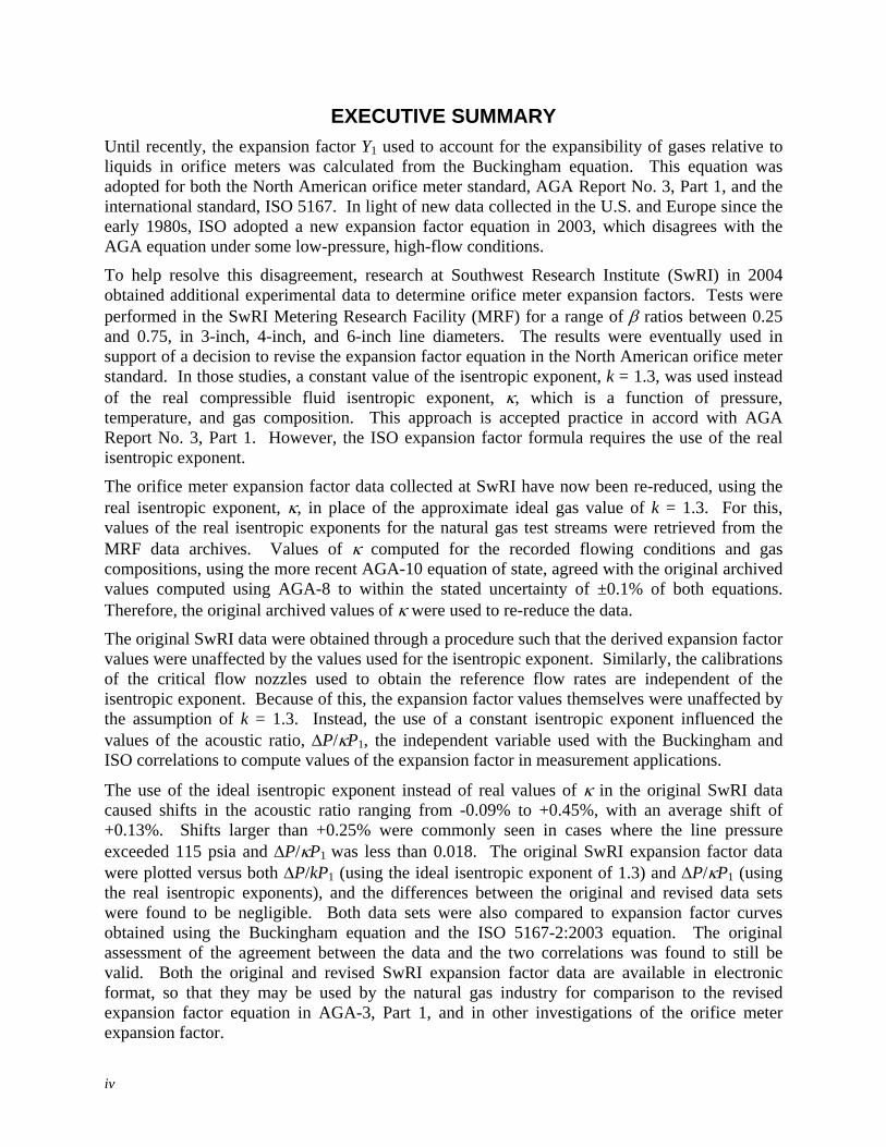
2.5 COMPARISON OF RESULTS Appendices A, B, and C contain plots of the data collected during the tests on the 3-inch, 4-inch, and 6-inch-diameter meter runs, respectively. The experimentally-determined expansion factors have been plotted versus ΔP/(κP1), using both the assumed value of 1.3 for κ and the value of the real isentropic exponents from the archived data. As in the original plots by Morrow (2004 and 2005), each value of Y1 represents the average of ten repeat runs at the same flow condition. Each value of Y1 is plotted versus the average value of ΔP/(κP1) over the ten repeat runs. Confidence intervals on the average Y1, at the 95% confidence level, have again been included in the plots. Confidence intervals of 0.093% in ΔP/(κP1), explained in Section 2.4.1, have been added to the data for this report. In nearly every case, these confidence intervals are smaller than the width of the symbol itself. A review of the graphs immediately reveals that the differences are negligible between ΔP/(kP1), with k = 1.3, and ΔP/(κP1), using the actual isentropic exponent. In all cases, the two sets of data fall almost on top of one another, and differences are nearly indistinguishable. The values of the real isentropic exponent, κ, were examined to confirm this, and the results are summarized in Table 2-1. All tests on a given orifice plate (described by meter line diameter and β ratio) were used to obtain a single value of the discharge coefficient for the plate. Accordingly, the extreme values of κ for all tests on a given orifice plate are listed in the table. Over all tests, the actual isentropic exponents ranged from 1.2976 to 1.3067. For these extreme cases, the approximate value of k = 1.3 would be in error by +0.18% and -0.51%, respectively. The average values of ΔP/(κP1) over each set of ten repeat runs were also reviewed, to quantify the effect of the assumption of k = 1.3. Table 2-2 lists the extremes of shifts in average values of ΔP/(κP1) when the acoustic ratio was calculated using k = 1.3 instead of the real isentropic exponents. The acoustic ratio shifted only by amounts ranging from -0.09% to +0.45%, with an average shift of +0.13%. This explains the minimal differences in the two sets of expansion factors when graphed as a function of ideal versus real isentropic exponents. The shifts in ΔP/κP1 became more positive with increasing line pressure and decreasing ΔP/κP1 for a given meter geometry. Shifts larger than +0.25% were commonly seen in cases where the line pressure exceeded 115 psia and ΔP/κP1 was less than 0.018. The graphs in the Appendices also compare the experimental data to the Buckingham equation and the ISO equation for the expansion factor. Morrow (2004) presented data from two test conditions as examples of the agreement between the test data and the two correlations. The results for those same test cases are shown again in Figure 2-2 through Figure 2-5, with the data graphed versus the acoustic ratio for both k = 1.3 and the actual isentropic exponents. The dashed lines correspond to the 95% confidence intervals in Y1 for each correlation, as reported by

8

AGA Report No. 3, Part 1 (American Gas Association, 2003) and Reader-Harris (1998). As the graphs show, because of the good agreement between the original and revised data, Morrow’s original comparisons between the data and the expansion factor equations are effectively unchanged by the use of the actual values of κ.

Table 2-1. Ranges of real values of isentropic exponents during the 2004 expansion factor tests at SwRI.

Extreme values of κ Line diameter β ratio Minimum Maximum 3 inches 0.60 1.3001 1.3056 0.67 1.3006 1.3059 0.75 1.3008 1.3043 4 inches 0.30 1.2984 1.3052 0.40 (new plate) 1.2976 1.3031 0.403 (old plate) 1.2994 1.3041 0.50 1.3005 1.3067 0.55 1.2987 1.3049 0.60 1.2981 1.3029 6 inches 0.25 1.2997 1.3057 0.30 1.3003 1.3057 0.35 1.3001 1.3055 0.40 1.3014 1.3055 0.45 1.3015 1.3043 0.45 (repeat test) 1.2980 1.3042

Table 2-2. Shifts in the average acoustic ratio, ΔP/(κP1), due to the use of a constant

value of k = 1.3 in calculations.

Shifts in ΔP/(κP1) Line diameter β ratio Minimum Average Maximum 3 inches 0.60 +0.10% +0.18% +0.39% 0.67 +0.12% +0.20% +0.41% 0.75 +0.12% +0.18% +0.31% 4 inches 0.30 –0.05% +0.06% +0.30% 0.40 (new plate) –0.09% –0.01% +0.18% 0.403 (old plate) 0.00% +0.09% +0.28% 0.50 +0.11% +0.21% +0.45% 0.55 0.00% +0.13% +0.34% 0.60 –0.09% –0.01% +0.17% 6 inches 0.25 +0.04% +0.15% +0.39% 0.30 +0.08% +0.19% +0.39% 0.35 +0.07% +0.17% +0.38% 0.40 +0.18% +0.24% +0.38% 0.45 +0.18% +0.22% +0.29% 0.45 (repeat test) –0.09% +0.02% +0.30%

9

0.950

0.955

0.960

0.965

0.970

0.975

0.980

0.985

0.990

0.995

1.000

0.00 0.02 0.04 0.06 0.08 0.10 0.12

ΔP/(k*P1)

Y1

MRF 4-inch nat. gas data- k=actualMRF 4-inch nat. gas data- k=1.3Buckingham equation95% Confidence Limits

Figure 2-2. Comparison of data from the 4-inch meter tube, β = 0.50, pressure tap #1,

using both k = 1.3 and actual values of κ, to the Buckingham correlation.


using both k = 1.3 and actual values of κ, to the ISO correlation.

10

0.960

0.965

0.970

0.975

0.980

0.985

0.990

0.995

1.000

0.00 0.01 0.02 0.03 0.04 0.05 0.06 0.07 0.08 0.09 0.10

ΔP/(k*P1)

Y1




0.960

0.965

0.970

0.975

0.980

0.985

0.990

0.995

1.000

0.00 0.01 0.02 0.03 0.04 0.05 0.06 0.07 0.08 0.09 0.10

(ΔP/k*P1)

Y1

MRF 6-inch nat. gas data- k=actualMRF 6-inch nat. gas data- k=1.3ISO 5167-2:2003 equation95% Confidence Limits



11

3. CONCLUSIONS In this report, the orifice meter expansion factor data collected at SwRI between 2003 and 2005 have been re-reduced, using the real isentropic exponent, κ, in place of the approximate ideal gas value of k = 1.3. For this work, values of the real isentropic exponent for the natural gas test streams, along with the temperature, pressure, and gas composition data used to determine them, were retrieved from the MRF data archives. Values of κ computed for the recorded flowing conditions, using the more recent AGA-10 equation of state, agreed with the original archived values computed using AGA-8 to within the stated uncertainty of ±0.1% of both equations. The SwRI expansion factor data were obtained by performing a linear regression of CdY1 versus the ratio of ΔP/P1, rather than a regression of CdY1 versus the acoustic ratio, ΔP/κP1. Similarly, the critical flow nozzles used in the SwRI expansion factor tests for reference flow rates have calibration curves that are independent of the isentropic exponent. Because of this, the expansion factor values themselves were unaffected by the assumption of a constant isentropic exponent. Instead, the use of k = 1.3 influenced the values of the acoustic ratio, ΔP/κP1, the independent variable used with the Buckingham and ISO correlations to compute values of the expansion factor in measurement applications. The use of the ideal isentropic exponent instead of real values of κ in the original SwRI data caused shifts in the acoustic ratio ranging from -0.09% to +0.45%. The original SwRI expansion factor data were plotted versus both ΔP/kP1 (using the ideal isentropic exponent of 1.3) and ΔP/κP1 (using the real isentropic exponents), and the differences between the original and revised data sets were judged to be negligible. Both data sets were also compared to expansion factor curves obtained using the Buckingham equation and the ISO 5167-2:2003 equation. The original assessment by Morrow (2004 and 2005) of the agreement between the data and the two correlations was found to be valid. Both the original and revised SwRI expansion factor data are available in electronic format, so that they may be used by the natural gas industry for comparison to the revised expansion factor equation in AGA-3, Part 1, and in other investigations of the orifice meter expansion factor.

12

REFERENCES American Gas Association Report No. 3, Orifice Metering of Natural Gas and Other Related Hydrocarbon Fluids, Part 1, General Equations and Uncertainty Guidelines, American Gas Association, Arlington, Virginia, USA, Third Edition, Second Printing, June 2003.

American Gas Association Report No. 8, Compressibility Factors of Natural Gas and Other Related Hydrocarbon Gases, American Gas Association, Arlington, Virginia, USA, Second Edition, Second Printing, July 1994.

American Gas Association Report No. 10, Speed of Sound in Natural Gas and Other Related Hydrocarbon Gases, American Gas Association, Arlington, Virginia, USA, January 2003.

Buckingham, E., "Notes on the Orifice Meter: The Expansion Factor for Gases," Bureau of Standards Journal of Research, Vol. 9, Research Paper No. 459, Washington, D.C., USA, 1932.

ISO 5167-1, Measurement of Fluid Flow by Means of Pressure Differential Devices – Part 1: Orifice Plates, Nozzles, and Venturi Tubes Inserted in Circular Cross-Section Conduits Running Full, International Organization for Standardization, Geneva, Switzerland, 1991.

ISO 5167-2, Measurement of Fluid Flow by Means of Pressure Differential Devices Inserted in Circular Cross-Section Conduits Running Full - Part 2: Orifice Plates, International Organization for Standardization, Geneva, Switzerland, 2003.

Morrow, T.B. (Southwest Research Institute), “Metering Research Facility Program: Orifice Meter Expansion Factor Tests in 4-Inch and 6-Inch Meter Tubes,” GRI Topical Report GRI-04/0042, Gas Technology Institute, Des Plaines, Illinois, USA, June 2004.

Morrow, T.B. (Southwest Research Institute), “Metering Research Facility Program: Additional Studies of Orifice Meter Installation Effects and Expansion Factor,” GRI Topical Report GRI-04/0246, Gas Technology Institute, Des Plaines, Illinois, USA, March 2005.

Reader-Harris, M., "The Equation for the Expansibility Factor for Orifice Plates," Proceedings of FLOMEKO 1998, Lund, Sweden, 1998.

13

APPENDIX A: REVISED EXPANSION FACTOR DATA, 3-INCH ORIFICE METER TUBE

0.9300.9350.9400.9450.9500.9550.9600.9650.9700.9750.9800.9850.9900.9951.000

0.00 0.02 0.04 0.06 0.08 0.10 0.12 0.14 0.16

ΔP/(k*P1)

Y1


Figure A-1. Comparison of data from the 3-inch meter tube, β = 0.60, pressure tap #1,


0.9300.9350.9400.9450.9500.9550.9600.9650.9700.9750.9800.9850.9900.9951.000

0.00 0.02 0.04 0.06 0.08 0.10 0.12 0.14 0.16

ΔP/(k*P1)

Y1




14

0.9300.9350.9400.9450.9500.9550.9600.9650.9700.9750.9800.9850.9900.9951.000

0.00 0.02 0.04 0.06 0.08 0.10 0.12 0.14 0.16

ΔP/(k*P1)

Y1




0.940

0.945

0.950

0.955

0.960

0.965

0.970

0.975

0.980

0.985

0.990

0.995

1.000

0.00 0.02 0.04 0.06 0.08 0.10 0.12 0.14

ΔP/(k*P1)

Y1




15

0.950

0.955

0.960

0.965

0.970

0.975

0.980

0.985

0.990

0.995

1.000

0.00 0.01 0.02 0.03 0.04 0.05 0.06 0.07 0.08 0.09 0.10

ΔP/(k*P1)

Y1




0.950

0.955

0.960

0.965

0.970

0.975

0.980

0.985

0.990

0.995

1.000

0.00 0.01 0.02 0.03 0.04 0.05 0.06 0.07 0.08 0.09 0.10

ΔP/(k*P1)

Y1




16

0.950

0.955

0.960

0.965

0.970

0.975

0.980

0.985

0.990

0.995

1.000

0.00 0.01 0.02 0.03 0.04 0.05 0.06 0.07 0.08 0.09 0.10

ΔP/(k*P1)

Y1




0.950

0.955

0.960

0.965

0.970

0.975

0.980

0.985

0.990

0.995

1.000

0.00 0.01 0.02 0.03 0.04 0.05 0.06 0.07 0.08 0.09 0.10

ΔP/(k*P1)

Y1




17

0.970

0.975

0.980

0.985

0.990

0.995

1.000

0.00 0.01 0.02 0.03 0.04 0.05 0.06

ΔP/(k*P1)

Y1




0.970

0.975

0.980

0.985

0.990

0.995

1.000

0.00 0.01 0.02 0.03 0.04 0.05 0.06

ΔP/(k*P1)

Y1




18

0.970

0.975

0.980

0.985

0.990

0.995

1.000

0.00 0.01 0.02 0.03 0.04 0.05 0.06

ΔP/(k*P1)

Y1




0.970

0.975

0.980

0.985

0.990

0.995

1.000

0.00 0.01 0.02 0.03 0.04 0.05 0.06

ΔP/(k*P1)

Y1




19

APPENDIX B: REVISED EXPANSION FACTOR DATA, 4-INCH ORIFICE METER TUBE

0.940

0.945

0.950

0.955

0.960

0.965

0.970

0.975

0.980

0.985

0.990

0.995

1.000

0.00 0.02 0.04 0.06 0.08 0.10 0.12 0.14 0.16

ΔP/(k*P1)

Y1


Figure B-1. Comparison of data from the 4-inch meter tube, β = 0.30, pressure tap #1,


0.940

0.945

0.950

0.955

0.960

0.965

0.970

0.975

0.980

0.985

0.990

0.995

1.000

0.00 0.02 0.04 0.06 0.08 0.10 0.12 0.14 0.16

ΔP/(k*P1)

Y1




20

0.940

0.945

0.950

0.955

0.960

0.965

0.970

0.975

0.980

0.985

0.990

0.995

1.000

0.00 0.02 0.04 0.06 0.08 0.10 0.12 0.14 0.16

ΔP/(k*P1)

Y1




0.940

0.945

0.950

0.955

0.960

0.965

0.970

0.975

0.980

0.985

0.990

0.995

1.000

0.00 0.02 0.04 0.06 0.08 0.10 0.12 0.14 0.16

ΔP/(k*P1)

Y1




21

Figure B-5. Comparison of data from the 4-inch meter tube, β = 0.40 (new plate),

pressure tap #1, using both k = 1.3 and actual values of κ, to the Buckingham correlation.

0.940

0.945

0.950

0.955

0.960

0.965

0.970

0.975

0.980

0.985

0.990

0.995

1.000

0.00 0.02 0.04 0.06 0.08 0.10 0.12 0.14

ΔP/(k*P1)

Y1



pressure tap #1, using both k = 1.3 and actual values of κ, to the ISO correlation.

22



0.950

0.955

0.960

0.965

0.970

0.975

0.980

0.985

0.990

0.995

1.000

0.00 0.02 0.04 0.06 0.08 0.10 0.12 0.14

ΔP/(k*P1)

Y1




23

0.940

0.945

0.950

0.955

0.960

0.965

0.970

0.975

0.980

0.985

0.990

0.995

1.000

0.00 0.02 0.04 0.06 0.08 0.10 0.12

ΔP/(k*P1)

Y1


Figure B-9. Comparison of data from the 4-inch meter tube, β = 0.403 (old plate),


0.940

0.945

0.950

0.955

0.960

0.965

0.970

0.975

0.980

0.985

0.990

0.995

1.000

0.00 0.02 0.04 0.06 0.08 0.10 0.12

ΔP/(k*P1)

Y1




24

0.950

0.955

0.960

0.965

0.970

0.975

0.980

0.985

0.990

0.995

1.000

0.00 0.02 0.04 0.06 0.08 0.10 0.12

ΔP/(k*P1)

Y1




0.950

0.955

0.960

0.965

0.970

0.975

0.980

0.985

0.990

0.995

1.000

0.00 0.02 0.04 0.06 0.08 0.10

ΔP/(k*P1)

Y1




25

0.950

0.955

0.960

0.965

0.970

0.975

0.980

0.985

0.990

0.995

1.000

0.00 0.02 0.04 0.06 0.08 0.10 0.12

ΔP/(k*P1)

Y1






26

0.950

0.955

0.960

0.965

0.970

0.975

0.980

0.985

0.990

0.995

1.000

0.00 0.02 0.04 0.06 0.08 0.10 0.12

ΔP/(k*P1)

Y1






27

0.950

0.955

0.960

0.965

0.970

0.975

0.980

0.985

0.990

0.995

1.000

0.00 0.01 0.02 0.03 0.04 0.05 0.06 0.07 0.08 0.09

ΔP/(k*P1)

Y1




0.950

0.955

0.960

0.965

0.970

0.975

0.980

0.985

0.990

0.995

1.000

0.00 0.01 0.02 0.03 0.04 0.05 0.06 0.07 0.08 0.09

ΔP/(k*P1)

Y1




28

0.950

0.955

0.960

0.965

0.970

0.975

0.980

0.985

0.990

0.995

1.000

0.00 0.01 0.02 0.03 0.04 0.05 0.06 0.07 0.08 0.09

ΔP/(k*P1)

Y1




0.950

0.955

0.960

0.965

0.970

0.975

0.980

0.985

0.990

0.995

1.000

0.00 0.01 0.02 0.03 0.04 0.05 0.06 0.07 0.08 0.09

ΔP/(k*P1)

Y1




29

0.970

0.975

0.980

0.985

0.990

0.995

1.000

0.00 0.01 0.02 0.03 0.04 0.05 0.06

ΔP/(k*P1)

Y1




0.970

0.975

0.980

0.985

0.990

0.995

1.000

0.00 0.01 0.02 0.03 0.04 0.05 0.06

ΔP/(k*P1)

Y1




30

0.970

0.975

0.980

0.985

0.990

0.995

1.000

0.00 0.01 0.02 0.03 0.04 0.05 0.06

ΔP/(k*P1)

Y1




0.970

0.975

0.980

0.985

0.990

0.995

1.000

0.00 0.01 0.02 0.03 0.04 0.05 0.06

ΔP/(k*P1)

Y1




31

APPENDIX C: REVISED EXPANSION FACTOR DATA, 6-INCH ORIFICE METER TUBE

0.940

0.945

0.950

0.955

0.960

0.965

0.970

0.975

0.980

0.985

0.990

0.995

1.000

0.00 0.02 0.04 0.06 0.08 0.10 0.12 0.14 0.16

ΔP/(k*P1)

Y1


Figure C-1. Comparison of data from the 6-inch meter tube, β = 0.25, pressure tap #1,


0.940

0.945

0.950

0.955

0.960

0.965

0.970

0.975

0.980

0.985

0.990

0.995

1.000

0.00 0.02 0.04 0.06 0.08 0.10 0.12 0.14 0.16

ΔP/(k*P1)

Y1




32

0.940

0.945

0.950

0.955

0.960

0.965

0.970

0.975

0.980

0.985

0.990

0.995

1.000

0.00 0.02 0.04 0.06 0.08 0.10 0.12 0.14 0.16

ΔP/(k*P1)

Y1




0.940

0.945

0.950

0.955

0.960

0.965

0.970

0.975

0.980

0.985

0.990

0.995

1.000

0.00 0.02 0.04 0.06 0.08 0.10 0.12 0.14 0.16

ΔP/(k*P1)

Y1




33

0.940

0.945

0.950

0.955

0.960

0.965

0.970

0.975

0.980

0.985

0.990

0.995

1.000

0.00 0.02 0.04 0.06 0.08 0.10 0.12 0.14

ΔP/(k*P1)

Y1




0.940

0.945

0.950

0.955

0.960

0.965

0.970

0.975

0.980

0.985

0.990

0.995

1.000

0.00 0.02 0.04 0.06 0.08 0.10 0.12 0.14

ΔP/(k*P1)

Y1




34

0.940

0.945

0.950

0.955

0.960

0.965

0.970

0.975

0.980

0.985

0.990

0.995

1.000

0.00 0.02 0.04 0.06 0.08 0.10 0.12 0.14

ΔP/(k*P1)

Y1




0.940

0.945

0.950

0.955

0.960

0.965

0.970

0.975

0.980

0.985

0.990

0.995

1.000

0.00 0.02 0.04 0.06 0.08 0.10 0.12 0.14

ΔP/(k*P1)

Y1




35

0.960

0.965

0.970

0.975

0.980

0.985

0.990

0.995

1.000

0.00 0.01 0.02 0.03 0.04 0.05 0.06 0.07 0.08 0.09 0.10

ΔP/(k*P1)

Y1




0.960

0.965

0.970

0.975

0.980

0.985

0.990

0.995

1.000

0.00 0.01 0.02 0.03 0.04 0.05 0.06 0.07 0.08 0.09 0.10

ΔP/(k*P1)

Y1




36

0.960

0.965

0.970

0.975

0.980

0.985

0.990

0.995

1.000

0.00 0.01 0.02 0.03 0.04 0.05 0.06 0.07 0.08 0.09 0.10

ΔP/(k*P1)

Y1




0.960

0.965

0.970

0.975

0.980

0.985

0.990

0.995

1.000

0.00 0.01 0.02 0.03 0.04 0.05 0.06 0.07 0.08 0.09 0.10

(ΔP/k*P1)

Y1




37





38





39





40





41

Figure C-21. Comparison of data from the 6-inch meter tube, β = 0.45 (repeat), pressure

tap #1, using both k = 1.3 and actual values of κ, to the Buckingham correlation.


tap #1, using both k = 1.3 and actual values of κ, to the ISO correlation.

42


tap #2, using both k = 1.3 and actual values of κ, to the Buckingham correlation.


tap #2, using both k = 1.3 and actual values of κ, to the ISO correlation.

Documents

REVISED ANALYSIS OF ORIFICE METER EXPANSION FACTOR · PDF fileREVISED ANALYSIS OF ORIFICE METER EXPANSION FACTOR DATA ... the effect of an assumption made during data reduction. In