PNNL-19525

Prepared for the U.S. Department of Energy Under Contract DE-AC05-76RL01830

Review of “Deepwater Horizon Release Estimate of Rate by PIV” Y Onishi June 2010

DISCLAIMER This report was prepared as an account of work sponsored by an agency of the United States Government. Neither the United States Government nor any agency thereof, nor Battelle Memorial Institute, nor any of their employees, makes any warranty, express or implied, or assumes any legal liability or responsibility for the accuracy, completeness, or usefulness of any information, apparatus, product, or process disclosed, or represents that its use would not infringe privately owned rights. Reference herein to any specific commercial product, process, or service by trade name, trademark, manufacturer, or otherwise does not necessarily constitute or imply its endorsement, recommendation, or favoring by the United States Government or any agency thereof, or Battelle Memorial Institute. The views and opinions of authors expressed herein do not necessarily state or reflect those of the United States Government or any agency thereof. PACIFIC NORTHWEST NATIONAL LABORATORY operated by BATTELLE for the UNITED STATES DEPARTMENT OF ENERGY under Contract DE-AC05-76RL01830 Printed in the United States of America Available to DOE and DOE contractors from the Office of Scientific and Technical Information,

P.O. Box 62, Oak Ridge, TN 37831-0062; ph: (865) 576-8401 fax: (865) 576-5728

email: reports@adonis.osti.gov Available to the public from the National Technical Information Service, U.S. Department of Commerce, 5285 Port Royal Rd., Springfield, VA 22161

ph: (800) 553-6847 fax: (703) 605-6900

email: orders@ntis.fedworld.gov online ordering: http://www.ntis.gov/ordering.htm

This document was printed on recycled paper.

(9/2003)

Review of “Deepwater Horizon Release Estimate of Rate by PIV” Y Onishi June 2010 Prepared for the U.S. Department of Energy under Contract DE-AC05-76RL01830 Pacific Northwest National Laboratory Richland, Washington 99352

PNNL-19525

4

Summary

General Comments:

The Plume Calculation Team (PCT) conducted high quality work within a very short period of

time, in spite of needing to use less than ideal quality videos provided by British Petroleum (BP), especially those made before the cutoff of the riser above the Blow Out Preventer (BOP) on June 3, 2010. There are at least two valid approaches for estimating the oil discharge coming out from the Deepwater Horizon broken pipeline and its riser, using BP videotapes. One method is to estimate the exit velocity directly with the use of the Particle Image Velocimetry (PIV). The second method is to use a buoyant plume analysis to determine the exit velocity. The PCT used both of these methods.

The PIV method focuses on phenomena in a very small local area where the mixture of oil and

gas is being released to the Gulf of Mexico. The oil-gas mixture generates several difficulties that the PCT needed to account for when applying the PIV method. Estimates of the oil discharge by five PCT members after the riser cut are quite consistent with each other, ranging 24,000 to 42,000 bbl/day for low estimates, and 40,000 to 49,000 bbl/day for the high estimates, as shown in Appendix 1 of the PCT report.

These estimates have some uncertainties. The fact that it is difficult to see the inside structure of

the oil-gas plume is a primary uncertainty. Another uncertainty is the velocity field in the local area, which varies significantly from one instance to another, necessitating the assumption that the phenomena shown on the videos are representative of the average condition. Some of the intensive turbulent-looking appearance of the plume may come from the fact that the oil and gas move upward at different velocities due to the different buoyancy, rather than solely from the turbulence of the jet flow itself. Vigorous interaction between gas and oil alters each phase’s pathline. However, this interfering effect may not be significant. It is because at the kink location just above the BOP, Jet J1 is more dominated by the inertia force than the buoyancy force, based on my estimate of the J1 jet’s densimetric Froude Number being 42, as discussed later. At the end of the riser, the oil/gas mixture coming out from the end of the riser is horizontal, thus the inertia force is horizontal and buoyancy force is vertically upward. Therefore, plumes of oil and gas have separate flow paths caused by buoyancy differences of within the plumes and ambient water, when there is not strong mixing between the oil and gas. As Appendix 6 states, the flow coming out at the end of the riser has three distinct mixtures; mostly oil alone, mostly gas alone, and a mixture of oil and gas, resulting in significant variation of the oil and gas ratio. As the PCT report correctly states, the much longer duration is needed to obtain the accurate averaged velocity of the oil plume.

Because the PIV method estimates the velocity near the outer edge of the buoyant plume, the

estimated velocity at the plume edge needs to be related to the velocity averaged over the plume cross section. For a free homogeneous jet, there are two distinct flow regions: the zone of the flow establishment, and the zone of the established flow. The total length of the zone of the flow establishment is expected to be around 6.2 times the nozzle diameter, but a buoyant plume has a shorter distance of this zone (Baumgarter and Trent 1970). Some of the PIV measurements were conducted within this zone, and the flow distribution is expected to be more like a top-hat shape, representing jet core and shearing areas. In the subsequent zone of the established flow, the normal (Gaussian) distribution is expected, as discussed in Appendix 7. For a single-phase buoyant plume (gas or oil alone), a normal (Gaussian) distribution is generally accepted for lateral distributions of the longitudinal velocity and the diluted concentration in the zone of the established flow (Stolzenbach and Harleman 1971). Although there are some uncertainties associated with the multi-phase oil-gas flow, it is possible to estimate the plume velocity averaged across the plume cross-section with the velocity of the plume edge estimated by the PIV method. The PCT members assigned the ratio of the average velocity to the plume edge velocity to

PNNL-19525

5

be between 1.5 and 3. This assumption is probably reasonable in light of many other uncertainties associated with the velocity estimates with the PIV. A second valid approach to estimate the oil plume exit velocity, thus the oil discharge rate, is to use a buoyant plume analysis (e.g., trajectory and width analyses) with and without the use of computational fluid dynamics codes. Appendix 7 shows the usefulness of this approach to estimate the oil discharge rate. This approach uses the overall behavior of the buoyant plume, as compared to the PIV method using a local plume velocity field.

There have been a large number of field measurements, laboratory hydraulic flume/basin experiments, and numerical models for a buoyant plume trajectory and mixing analysis associated with heated water and sewage/industrial waste effluents released to surface waters (Abraham1963, Fan and Brooks 1969, Sharazi and Davis 1972). Although there are some recent studies, most of the cited studies have been conducted in 1960s to mid 1970s. One caution when using this approach to estimate oil discharge rate, is that the plume trajectory is very sensitive to the ambient flow. Although there may be some intermittent ambient flows in this depth, it is reasonable to assume (at least initially) that the ambient flow velocity at the bottom of the Guff of Mexico at 5,000 ft deep is almost zero. However, Appendix 6 indicates that the ambient velocity there may be 0.1 ~ 0.2 m/s due to the existence of the trench. If the actual ambient flow is horizontal, the computed plume trajectory with the assumption of a stagnant ambient flow would significantly overestimate the plume inertia at the end of the riser to match the observed oil plume trajectory. This leads to the significant overestimation of the plume exit velocity, thus, the oil discharge rate. If the actual ambient flow is more vertical, the computed plume trajectory with a stagnant ambient flow significantly overestimates the plume buoyancy to match the observed oil plume trajectory. This leads to the significant underestimation of the plume exit velocity, thus, the oil discharge rate. Beside plume exit velocity measurements suggested in Appendix 6, velocity measurements of the ambient flow may also be needed.

A computational fluid dynamics code must include all major mechanisms of the oil transport and

fate, if it is to be applied to the oil plume dispersion in a wide area for long transients. These phenomena include the rising of oil droplets of multiple sizes (with the use of oil dispersant) and oil emulsion.

It is generally better to use various different approaches to estimate the oil discharge rate, because

each has its own limitations and uncertainties. I added some additional ways to evaluate the oil discharge rate.

As I stated at the beginning, the PCT has conducted a credible job by employing various assessment methods within the short period of time with the materials supplied to them.

PNNL-19525

6

Specific Comments:

Subsection 2.2.1 of Appendix 4 states that the estimated centerline jet velocity is 3 m/s at 70 cm away from the 2.4-cm diameter opening. By using Equation 6 of Appendix 4, the plume exit velocity is calculated to be 85 m/s, assuming the plume is homogeneous. This leads to the oil discharge of 3,400 m3/day, as reported in the appendix.

The centerline velocity is usually expressed as (Wiegel 1964)

x

D

U

UC 2.60

(1)

where, UC = centerline jet velocity U0 = jet nozzle velocity D = nozzle diameter x = downstream distance. Equation 1 with the centerline velocity of 3 m/s at 70 cm away yields the jet nozzle velocity of 14 m/s, not 85 m/s. Please clarify this point.

Subsection 3.3 states that the flow is inertia dominated because of the estimated high Reynolds Number. As I will discuss later in this review write-up, the oil plume at the end of the riser (at least what I saw briefly) appears to be a strongly buoyant plume, although the inertia force of the oil plume may still be somewhat greater than the buoyancy force with the estimated densimetric Froude Number being greater than one. Appendix 6 describes the proposed experiment. I support that well thought-out field measurements will be conducted at the oil spill site to reduce a large amount of uncertainties described in the PCT report. In Appendix 7, for the velocity estimate using the PIV method, the velocity at the edge of the plume is assumed to be the average velocity across the plume cross-section. With this assumption, the oil discharge rate at the end of the riser was estimated to be 55,000 bbl/day. This estimate is very conservative as the maximum oil discharge estimate. Other PCT members used the plume average velocity to be 1.5 to 3 times the velocity estimated at the plume edge. The distance from the riser end was reported to be 0.8 m, which is 2.3 times the 13.75-inch diameter of the riser. Thus, this location is likely to be in the zone of the flow establishment of this plume jet, and I expect that the average velocity to be closer to 1.5 times the velocity of the plume edge than 3 times. With the average velocity to be 1.5 times of the velocity estimated at the plume edge, it would be 83,000 bbl/day, instead of 55,000 bbl/day, as reported in Appendix 7. This is also true for the oil discharge estimate at the kink location based on the velocity estimate at 60 cm downstream. If the J1 jet opening diameter is 1.9 cm, as Appendix 7 indicates, this location is 32 times the jet exit diameter from the opening. Thus, it is in the zone of the established flow, and the velocity distribution is expected to a Gaussian distribution, as Appendix 7’s Approach 2 also indicates. Thus, the ratio of the average jet velocity across the plume cross-section to the plume edge velocity is closer to 3 than 1.5. Appendix 7 also assumes that the total oil flow rate from the riser kink jets to be twice of the oil discharge of the J1 jet. Subsection 3.1 of Appendix 4 states that the jets J and J2 are stronger than J1. Is it better to assume that the total oil discharge is about three times the J1 discharge?

PNNL-19525

7

These two points imply that the oil discharge estimates reported under Approach 1 of Appendix 7 seem very conservative as maximum oil discharge estimates.

I strongly support a plume analysis to be a part of the oil spill assessment, as performed under Analysis Approaches 2 and 3 of Appendix 7. It should cover both the close proximity of the BOP/the end of the riser in a short-term, and regional-scale in the longer time frame. Analysis Approach 2 of Appendix 7 describes three different methods; the first method is based on the ambient flow entrainment, the second method uses the pressure drop across the kink, and the third is based on the plume trajectory angle. The first method led to a conclusion that the oil-gas mixture is diluted by 6.7 times by the ambient water, and its plume width is 30 cm (16 times the kink opening diameter of 1.9 cm) at 60 cm downstream (32 times the kink opening diameter). These values at 60 cm downstream are consistent with the dilution and the plume width I estimated with different approaches, as discussed here.

The rise and mixing of a buoyant effluent discharged through a submerged outfall in stagnant,

non-stratified ambient water is governed by the buoyancy and inertia forces of the effluent, and is commonly expressed as a function of the following densimetric Froude Number:

gD

UF

a

Ja

D

0 (2)

where, D = Effluent outlet nozzle diameter FD = Densimetric Froude Number g = Gravitational acceleration U0 = Effluent nozzle velocity a = Ambient water density J = Effluent density at the nozzle.

With D = 1.9 cm, U0 = 14 m/s, a = 1028 kg/m3 , J = 413 kg/m3 (a 50-50 mixture of oil and gas indicated in Appendix 7), the densimetric Froude Number, FD is 42. Thus, the jet is driven mostly by the inertia force, not much by the buoyancy force. Thus, this plume is close to a homogeneous free jet. Predicted dilution of a jet discharged vertically into a stagnant non-stratified ambient water is presented in Figure 1 (Sharazi and Davis 1972).

PNNL-19525

8

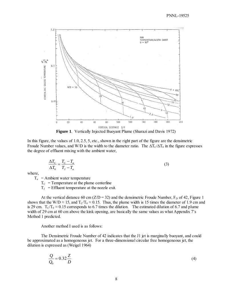
Figure 1. Vertically Injected Buoyant Plume (Sharazi and Davis 1972)

In this figure, the values of 1.0, 2.5, 5, etc., shown in the right part of the figure are the densimetric Froude Number values, and W/D is the width to the diameter ratio. The TC/T0 in the figure expresses the degree of effluent mixing with the ambient water,

aJ

aCC

TT

TT

T

T

0

(3)

where, Ta = Ambient water temperature

TC = Temperature at the plume centerline TJ = Effluent temperature at the nozzle exit. At the vertical distance 60 cm (Z/D = 32) and the densimetric Froude Number, FD of 42, Figure 1

shows that the W/D ≈ 15, and TC/T0 ≈ 0.15. Thus, the plume width is 15 times the diameter of 1.9 cm and is 29 cm. TC/T0 ≈ 0.15 corresponds to 6.7 times the dilution. The estimated dilution of 6.7 and plume width of 29 cm at 60 cm above the kink opening, are basically the same values as what Appendix 7’s Method 1 predicted.

Another method I used is as follows:

The Densimetric Froude Number of 42 indicates that the J1 jet is marginally buoyant, and could be approximated as a homogeneous jet. For a three-dimensional circular free homogeneous jet, the dilution is expressed as (Weigel 1964)

D

Z

Q

Q 32.00

(4)

PNNL-19525

9

where, Q = Flow rate at distance Z Q0 = Jet discharge at the nozzle exit. Thus, at Z = 60 cm (Z/D = 32), the discharge of the diluted jet is 10 times greater than the initial plume discharge. Thus, the dilution is 10 times.

These values, using the two methods I employed here, are similar to the values reported in Appendix 7. Method 2 used under Analysis Approach 2 of Appendix 7 depends on the value of the pressure drop across the JI jet opening. Unless 400 psi pressure drop used in the analysis was actually a measured value across the J1 jet opening, there is a large uncertainty on the pressure drop estimate of 400 psi. There is a large uncertainty on the pressure drop through a well from the oil reservoir to the sea bottom. Thus, I consider Method 1 based on the plume entrainment assessment has a greater probability of being more accurate than Method 2 based on the pressure drop. Method 3, Analysis Approach 2 of Appendix 7, uses somewhat similar approach to what I used, as described below. The modified Froude Number defined in Appendix 7 is different from more common definition of the densimetric Froude Number shown in Equation 2 here. Please define parameters, 0 and ∞ of the modified Froude Number. The left plot of Figure 13 in Appendix 7 shows a reasonable match between the actual plume and the predicted plume trajectory. However, the estimated oil discharge of 86,000 bbl/day is much greater than what I estimated as described below. The actual plume rise shown in this plot rose less sharply than the one I saw on Yahoo.com and used. Thus Appendix 7’s oil discharge estimate is much greater than my estimate. This discrepancy may be a reflection of the temporal variability of the plume coming out from the end of the riser.

Analysis Approach 3 of Appendix 7 describes an application of the commercially available

computational fluid dynamics code, FLUENT, showing a good match between the observed and predicted plume dispersion.

FLUENT has been widely used to solve a wide range of fluid dynamic problems. However, I

anticipate that an FLUENT application to this oil spill condition in a regional-scale and longer term may face a strong challenge to handle multiple-size oil droplets by simultaneously solving a multiple set of Navier Stokes Equations for oil droplets of each size and the ambient flow, and simulating the momentum exchange among each of these oil droplets and ambient water. Appendix 8 states that the Jet J1 is a main jet coming out at the kink riser above the BOP. Please see my above comment of Jets, J, J2 and J1. Independent of the PCT effort, I estimated the possible oil flow discharge rate at the end of the riser with a plume trajectory analysis and a video I saw on yahoo.com, as I will briefly described here. My estimate provides a rough estimate of the oil discharge rate for comparison with the PCT report information. The mixing trajectory of a buoyant plume discharged horizontally through a submerged outfall in stagnant, non-stratified ambient water is governed by the buoyancy and inertia forces of the effluent, as shown in Figure 2 (Sharazi and Davis 1972):

PNNL-19525

10

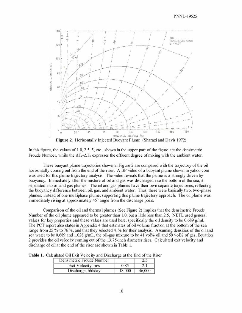
Figure 2. Horizontally Injected Buoyant Plume (Sharazi and Davis 1972)

In this figure, the values of 1.0, 2.5, 5, etc., shown in the upper part of the figure are the densimetric Froude Number, while the TC/T0 expresses the effluent degree of mixing with the ambient water.

These buoyant plume trajectories shown in Figure 2 are compared with the trajectory of the oil horizontally coming out from the end of the riser. A BP video of a buoyant plume shown in yahoo.com was used for this plume trajectory analysis. The video reveals that the plume is a strongly driven by buoyancy. Immediately after the mixture of oil and gas was discharged into the bottom of the sea, it separated into oil and gas plumes. The oil and gas plumes have their own separate trajectories, reflecting the buoyancy difference between oil, gas, and ambient water. Thus, there were basically two, two-phase plumes, instead of one multiphase plume, supporting this plume trajectory approach. The oil plume was immediately rising at approximately 45° angle from the discharge point.

Comparison of the oil and thermal plumes (See Figure 2) implies that the densimetric Froude Number of the oil plume appeared to be greater than 1.0, but a little less than 2.5. NETL used general values for key properties and these values are used here, specifically the oil density to be 0.689 g/mL. The PCT report also states in Appendix 4 that estimates of oil volume fraction at the bottom of the sea range from 25 % to 76 %, and that they selected 41% for their analysis. Assuming densities of the oil and sea water to be 0.689 and 1.028 g/mL, the oil-gas mixture to be 41 vol% oil and 59 vol% of gas, Equation 2 provides the oil velocity coming out of the 13.75-inch diameter riser. Calculated exit velocity and discharge of oil at the end of the riser are shown in Table 1. Table 1. Calculated Oil Exit Velocity and Discharge at the End of the Riser

Densimetric Froude Number 1 2.5 Exit Velocity, m/s 0.85 2.1 Discharge, bbl/day 18,000 46,000

PNNL-19525

11

Table 1 indicates that the very rough estimate of the oil discharge out of the end of the riser is around 46, 000 bbl/day. This assumes that the densimetric Froude Number is 2.5, based on the single videotape. If the densimetric Froude Number is 1.0, the average oil discharge from the end of the riser is approximately 18, 000 bbl/day. The estimates of oil release rate from the end of the riser are very rough and have many uncertainties, including:

The video shows only the short distance of the plume trajectory out of the end of the riser. The plume of oil outside of the riser was assumed to be a single-phase. The ambient flow was assumed be stagnant in the immediately vicinity of the riser. No ambient stratification was assumed near the riser. The plume model predictions are for heated water, and industrial and municipal wastes. Heated

water mixes relatively easily with water. However, industrial and municipal wastes are more difficult to mix with water, and are somewhat similar to oil in this respect.

The mixture of the oil and water change the viscosity of the mixture much more than heated water does.

References

Abraham. G. 1963. “Jet Diffusion in Stagnant Ambient Fluid,” Delft Hydraulics Publication No. 29, Delft Hydraulic Laboratory, Delft, The Netherlands. Baumgarter, D.J., and D.S. Trent. 1970. “Ocean Outfall Design Part 1. Literature Review and Theoretical Development,” U.S. Department of the Interior, federal Water Quality Administration, Northwest Region, Pacific Northwest Water Laboratory, Corvallis, Oregon. Fan, L-N and N.H. Brooks. 1969. “Numerical Solution of Turbulent Buoyant Jet Problems,” Technical Publication No. KH-R-18, W.M. Keck Laboratory of Hydraulics and Water Resources, Division of Engineering and Applied Sciences, California Institute of Technology, Pasadena, California. Shirazi, M.A. and L.R. Davis. 1972. “Workbook of Thermal Plume Prediction, Volume 1. Submerged Discharge,” EPA-R2-72-005a, The U.S. Environmental protection Agency, Pacific Northwest Water Laboratory, National Environmental Research Center, Corvallis, Oregon. Stolzenbach, K.D., and D.R.F. Harleman. 1971. “An Analytical and Experimental Investigation of Surface Discharges of Heated Water,” Report No. 135. Ralph M. Parsons Hydraulic Laboratory, Massachusetts Institute of Technology, Cambridge, Massachusetts. Wiegel, R.L. 1964, Oceanographical Engineering, Prentice-Hall Inc., Englewood Cliff, New Jersey