Review: DP and Econometrics - MIT OpenCourseWare · PDF fileReplicate the chosen payoff using dynamic trading in available assets. Merton’s solution: CRRA utility with risk aversion

Dynamic Portfolio Choice Financial Econometrics

Review: DP and Econometrics

Leonid Kogan

MIT, Sloan

15.450, Fall 2010

� Leonid Kogan ( MIT, Sloan ) Review: Part II 15.450, Fall 2010 1 / 22c


Outline

1

2

Dynamic Portfolio Choice

Financial Econometrics

c� Leonid Kogan ( MIT, Sloan ) Review: Part II 15.450, Fall 2010 2 / 22


Outline

1

2





Portfolio Choice: Static Approach

In models in which all options are redundant (e.g., Black-Scholes), dynamic portfolio choice is relatively easy. Solve a static problem:

Find the best state contingent payoff (under given utility) which is budget-feasible. Replicate the chosen payoff using dynamic trading in available assets.

Merton’s solution: CRRA utility with risk aversion γ, Black-Scholes model:

φ� µ − r = t γσ2

Myopic portfolio is optimal.



Problem

Consider the Black-Scholes framework with parameters r , µ, and σ. Yourbjective is to find an optimal investment strategy maximizing the expectedtility of terminal portfolio value

E0

[1 1(W

1 T )−γ

− γ

]ubject to a lower bound on terminal wealth:

WT > W

ou

s

1 Using the static approach, express the optimal terminal wealth as a function ofthe SPD.Show that one can implement the optimal strategy using European options onthe stock.(*) Implement the optimal strategy using dynamic trading.

2

3

c© Leonid Kogan ( MIT, Sloan ) Review: Part II 15.450, Fall 2010 5 / 22


DP

Dynamic programming principle.

Bellman equation.

Controlled Markov processes. Problem formulation.

Key examples: portfolio choice with time-varying moments of returns; American option pricing.



Outline

1

2




� �

�


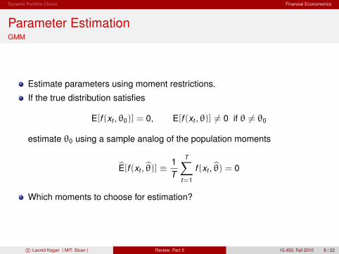
Parameter Estimation GMM

Estimate parameters using moment restrictions.

If the true distribution satisfies

E[f (xt , θ0)] = 0, E[f (xt , θ)] = 0 if θ = θ0

estimate θ0 using a sample analog of the population moments

1 T

E�[f (xt , θ�)] ≡ f (xt , θ�) = 0T

t=1

Which moments to choose for estimation?



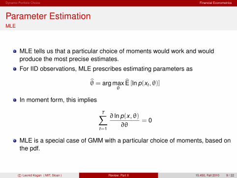
Parameter Estimation MLE

MLE tells us that a particular choice of moments would work and wouldproduce the most precise estimates.

For IID observations, MLE prescribes estimating parameters as

θ� = arg max E� [ln p(xt , θ)] θ

In moment form, this implies

T� ∂ ln p(x , θ) = 0

∂θ t=1

MLE is a special case of GMM with a particular choice of moments, based on the pdf.


� � �


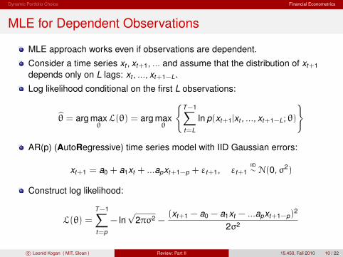
MLE for Dependent Observations

MLE approach works even if observations are dependent.

Consider a time series xt , xt+1, ... and assume that the distribution of xt+1

depends only on L lags: xt , ..., xt+1−L.

Log likelihood conditional on the first L observations:

T −1

θ� = arg max L(θ) = arg max ln p(xt+1|xt , ..., xt+1−L; θ) θ θ

t=L

AR(p) (AutoRegressive) time series model with IID Gaussian errors:

IID xt+1 = a0 + a1xt + ...apxt+1−p + εt+1, εt+1 ∼ N(0, σ2)

Construct log likelihood:

� (xt+1 − a0 − a1xt − ...apxt+1−p)2

L(θ) = T −1

− ln √

2πσ2 − 2σ2

t=p



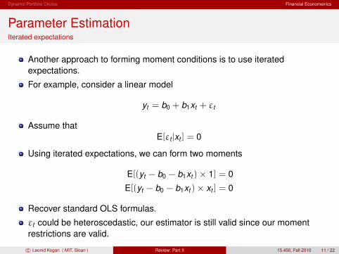
Parameter Estimation Iterated expectations

Another approach to forming moment conditions is to use iteratedexpectations.

For example, consider a linear model

yt = b0 + b1xt + εt

Assume thatE[εt |xt ] = 0

Using iterated expectations, we can form two moments

E[(yt − b0 − b1xt ) × 1] = 0

E[(yt − b0 − b1xt ) × xt ] = 0

Recover standard OLS formulas.

εt could be heteroscedastic, our estimator is still valid since our moment restrictions are valid.

c Review: Part II 11 / 22 � Leonid Kogan ( MIT, Sloan ) 15.450, Fall 2010


Parameter Estimation QMLE

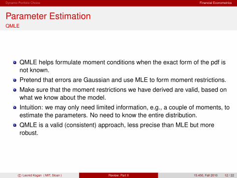
QMLE helps formulate moment conditions when the exact form of the pdf is not known.

Pretend that errors are Gaussian and use MLE to form moment restrictions.

Make sure that the moment restrictions we have derived are valid, based on what we know about the model.

Intuition: we may only need limited information, e.g., a couple of moments, to estimate the parameters. No need to know the entire distribution.

QMLE is a valid (consistent) approach, less precise than MLE but morerobust.


��


Example: Interest Rate Model Iterated expectations

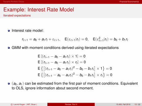
Interest rate model:

rt+1 = a0 + a1rt + εt+1, E(εt+1|rt ) = 0, E(ε2 t+1|rt ) = b0 + b1rt

GMM with moment conditions derived using iterated expectations

E [(rt+1 − a0 − a1rt ) × 1] = 0

E [(rt+1 − a0 − a1rt ) × rt ] = 0

E (rt+1 − a0 − a1rt )2 − b0 − b1rt × 1 = 0

E (rt+1 − a0 − a1rt )2 − b0 − b1rt × rt = 0

(a0, a1) can be estimated from the first pair of moment conditions. Equivalent to OLS, ignore information about second moment.



Example: Interest Rate Model QMLE

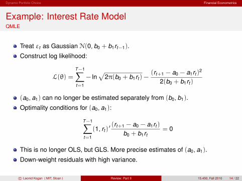
Treat εt as Gaussian N(0, b0 + b1rt−1).

Construct log likelihood:

T −1� � (rt+1 − a0 − a1rt )2

L(θ) = − ln 2π(b0 + b1rt ) − 2(b0 + b1rt )t=1

(a0, a1) can no longer be estimated separately from (b0, b1).

Optimality conditions for (a0, a1):

T −1� (rt+1 − a0 − a1rt )(1, rt )

� = 0b0 + b1rtt=1

This is no longer OLS, but GLS. More precise estimates of (a0, a1).

Down-weight residuals with high variance.

c Review: Part II 14 / 22 � Leonid Kogan ( MIT, Sloan ) 15.450, Fall 2010


GMM Standard Errors IID Observations

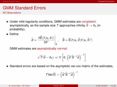
Under mild regularity conditions, GMM estimates are consistent: asymptotically, as the sample size T approaches infinity, θ� θ0 (in→probability).

Define �d� =

∂E�(f (xt , θ)) �� , S� = E�[f (xt , θ�)f (xt , θ�)�]∂θ � �

θ�GMM estimates are asymptotically normal:

√T (θ�− θ0) ⇒ N

�

0, �

d� �S�−1d��−1 �

Standard errors are based on the asymptotic var-cov matrix of the estimates, � �−1 T Var[θ�] = d� �S�−1d�



Problem

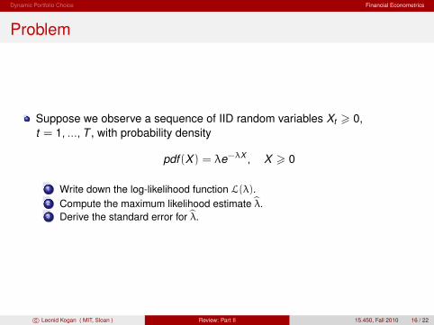
Suppose we observe a sequence of IID random variables Xt > 0,t = 1, ...,T , with probability density

pdf (X ) = λe−λX , X > 0

1 Write down the log-likelihood function L(λ).Compute the maximum likelihood estimate λ̂.Derive the standard error for λ.

2

3 ̂



Problem

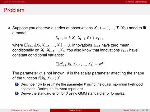
Suppose you observe a series of observations Xt , t = 1, ...,T . You need to fita model

Xt+1 = f (Xt ,Xt−1; θ) + εt+1

where E[εt+1|Xt ,Xt−1, ...,X1] = 0. Innovations εt+1 have zero meanconditionally on Xt , Xt−1,...,X1. You also know that innovations εt+1 haveconstant conditional variance:

E 2 2[ε |t+1 Xt ,Xt−1, ...,X1] = σ

The parameter σ is not known. θ is the scalar parameter affecting the shapeof the function f (X ,X ; θ).t t−1

1 Describe how to estimate the parameter θ using the quasi maximum likelihoodapproach. Derive the relevant equations.Derive the standard error for θ using GMM standard error formulas.2 ̂


�


GMM Standard Errors Dependent observations

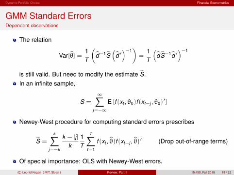
The relation

1 � � �−1

� 1 � �−1

Var[θ�] = d�−1S� d� � = d�S�−1d� �T T

is still valid. But need to modify the estimate S�. In an infinite sample,

∞S = E [f (xt , θ0)f (xt−j , θ0)

�] j=−∞

Newey-West procedure for computing standard errors prescribes

k T� k − |j | 1 � S� = f (xt , θ�)f (xt−j , θ�) � (Drop out-of-range terms)

k T j=−k t=1

Of special importance: OLS with Newey-West errors.


� � � �


Additional Results

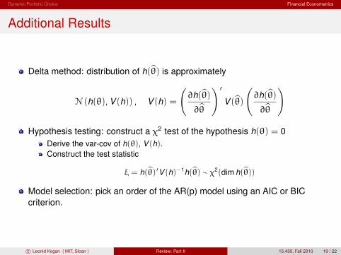
Delta method: distribution of h(θ�) is approximately

∂h(θ�) � ∂h(θ�)

N (h(θ), V (h)) , V (h) = V (θ�) ∂θ� ∂θ�

Hypothesis testing: construct a χ2 test of the hypothesis h(θ) = 0 Derive the var-cov of h(θ), V (h). Construct the test statistic

ξ = h(θ�) �V (h)−1h(θ�) ∼ χ2(dim h(θ�)) Model selection: pick an order of the AR(p) model using an AIC or BIC criterion.


� � � �


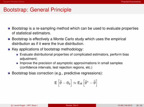
Bootstrap: General Principle

Bootstrap is a re-sampling method which can be used to evaluate properties of statistical estimators.

Bootstrap is effectively a Monte Carlo study which uses the empiricaldistribution as if it were the true distribution.Key applications of bootstrap methodology:

Evaluate distributional properties of complicated estimators, perform bias adjustment; Improve the precision of asymptotic approximations in small samples (confidence intervals, test rejection regions, etc.)

Bootstrap bias correction (e.g., predictive regressions):

E θ�− θ0 ≈ ER θ�� − θ�



Boostrap Confidence Intervals

Basic bootstrap confidence interval. Nonparametric approach in IID samples.

For non-IID samples, use parametric bootstrap.



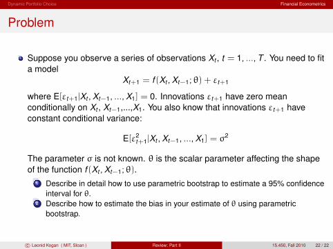
Problem

Suppose you observe a series of observations Xt , t = 1, ...,T . You need to fita model

Xt+1 = f (Xt ,Xt−1; θ) + εt+1

where E[εt+1|Xt ,Xt−1, ...,X1] = 0. Innovations εt+1 have zero meanconditionally on Xt , Xt−1,...,X1. You also know that innovations εt+1 haveconstant conditional variance:

E 2[ε |t+1 Xt ,X 2t−1, ...,X1] = σ

The parameter σ is not known. θ is the scalar parameter affecting the shapeof the function f (Xt ,Xt−1; θ).

1 Describe in detail how to use parametric bootstrap to estimate a 95% confidenceinterval for θ.Describe how to estimate the bias in your estimate of θ using parametricbootstrap.

2


MIT OpenCourseWarehttp://ocw.mit.edu

15.450 Analytics of Finance Fall 2010

For information about citing these materials or our Terms of Use, visit: http://ocw.mit.edu/terms .

http://ocw.mit.edu

http://ocw.mit.edu

Documents

Review: DP and Econometrics - MIT OpenCourseWare · PDF fileReplicate the chosen payoff using dynamic trading in available assets. Merton’s solution: CRRA utility with risk aversion