Resource Flows Among Three Generations in Guatemala Study (2007–08):

Definitions, tracking, data collection, coverage, and attrition by

Paúl Melgar1 Luis Fernando Ramírez1

Scott McNiven2 Rosa Mery Mejía1 Ann DiGirolamo3 John Hoddinott2

John A. Maluccio4

June 2008

MIDDLEBURY COLLEGE ECONOMICS DISCUSSION PAPER NO. 08-03

DEPARTMENT OF ECONOMICS MIDDLEBURY COLLEGE

MIDDLEBURY, VERMONT 05753

http://www.middlebury.edu/~econ

1

Resource Flows Among Three Generations in Guatemala Study (2007–08): Definitions, tracking, data collection, coverage, and attrition

Paúl Melgar1

Luis Fernando Ramírez1 Scott McNiven2

Rosa Mery Mejía1 Ann DiGirolamo3 John Hoddinott2

John A. Maluccio4

June 2008 Abstract: The allocation of resources across generations and the consequences of these allocations represent a research agenda with significant policy implications. At the same time, their empirical investigation imposes immense data requirements, and therefore data collection challenges. In this paper, we describe how we met these challenges, in the Resource Flows Among Three Generations in Guatemala Study, or IGT, carried out in 2006–07. In doing so, we provide a guide for using and interpreting the data collected as part of IGT, as well as an example for others interested in implementing research projects on similar themes elsewhere. Complex research topics, across generations and across a range of possible measures of well-being, led to a relatively complicated sample selection process and survey design, with component modules that were applicable to different “types” of sample members, depending on their generational status and age, and who often lived in different locations. It also led to a wide set of survey domains, ranging from economic, educational, and psychological surveys to clinical medical exams for both the young and the elderly. Survey coverage was above 85% of the targeted sample for most categories of respondents and most modules, and a number of safeguards were in place to ensure high quality data. Biases due to attrition, measured against the original 1970s rounds of survey work upon which IGT built, while present, should not reduce substantially the validity of research findings to come from this rich sample. The extent to which this is true, though, may vary depending on the topic under consideration and the controls included in the analyses. 1 Institute for Nutrition in Central America and Panama, Guatemala City, Guatemala 2 International Food Policy Research Institute, Washington DC 3 Department of Global Health, Rollins School of Public Health, Emory University, Atlanta GA 4 Department of Economics, Middlebury College, Middlebury VT Acknowledgments: We gratefully acknowledge the financial support of the US National Institute of Child Health and Human Development (Grant: 5R01HD045627-05) for present activities and the many organizations (US National Institute of Health, US National Science Foundation, Thrasher Research Fund, and Nestle Foundation) that have funded research based on the INCAP Longitudinal Study since its inception. We also have benefited from the support of the National Institutes of Aging (Grant: P30 AG12836), the Boettner Center for Pensions and Retirement Security at the University of Pennsylvania, and the Mellon Foundation grant to the Population Studies Center of the University of Pennsylvania. Finally, the investigators thank the participants of the INCAP Longitudinal Study, and their families, for their cooperation and past investigators and staff for establishing and maintaining this valuable sample.

2

1. Introduction Rising life expectancy and falling fertility rates are leading to marked increases in the proportion of elderly persons in most countries of the world. While this phenomenon is the subject of extensive analysis and policy debate in developed countries, it has received comparatively little attention in developing countries, despite the fact that the proportion of the elderly in developing country populations already has grown substantially and is projected to treble by 2050, and increase by even more in Latin America (Behrman, Duryea, and Székely 2003; United Nations 2001). At the same time that the life spans have been increasing, however, there has been disappointingly slow progress in many developing countries in improving nutrition, health, and schooling of the youngest generations. As a result, in both the public and private domains, critical time-sensitive investments in children increasingly compete with the need to support the elderly.

In Guatemala, for example, from 1969 to 2002, life expectancy rose from 53 to 68 years for women and from 51 to 62 years for men, yet in 2002, 50% of children under age five were stunted (with height-for-age z-score less than -2). Similarly, although there have been recent improvements in primary schooling, outcomes at the secondary school level remain poor, with less than 50% of 15 year-olds enrolled in 2006 (Behrman, Duryea, and Maluccio 2008). These levels and trends form the backdrop to the Resource Flows Among Three Generations in Guatemala Study, carried out in 2006–07. In this paper we introduce this new study, which we refer to as the IGT Study (2006–07), an acronym for “intergenerational transfers.”

The objective underlying IGT is to improve understanding of the roles played by public policy, private resources, preferences, exogenous shocks, and markets—as well as the interactions among these factors—in the allocation of resources, and their consequences for well-being, across three generations in Guatemala. To meet this objective, we collected information along three dimensions relevant to the multiple roles of resource allocations and their possible effects.

The first was the resource types and allocations themselves across generations. Prime-age adults with both children and elderly parents face a trade-off in the allocation of time dedicated to work, elder care, child care, and leisure. They also face consequential decisions regarding the allocation of income to their own consumption, to meeting the consumption needs of their elderly parents, and to investments in the human capital of their children.

The second aspect was the potential impacts of these resource allocations on individual well-being, particularly for the elderly and the young. We view well-being as a multifaceted concept, and therefore took a comprehensive, as well as age-specific, approach in assessing it. For the elderly, we collected information on their physical and mental health, access to preventative/curative health care, satisfaction with health status, social resources, and economic resources. For the young, we included indicators of health, nutrition, cognitive skills, schooling, and adequate care.

A third aspect underlying the data collection was gender, since it likely plays an important role in intergenerational allocations (de Tejada, Mazariegos, and Barrios 2005). For example, forms of interactions between middle-generation individuals and elderly parents, or parents-in-law, often differ by gender. Alternatively, parents’ allocations to their children may vary by gender, particularly where returns to schooling differ by gender or where parents have different preferences for sons and daughters.

3

The allocation of resources across generations and the consequences of these allocations represent a research agenda with significant policy implications. At the same time, their empirical investigation imposes immense data requirements, and therefore data collection challenges. In this paper, we describe how we met these challenges, building on a well-known study from Guatemala. We begin by explaining how we defined the study sample and how we located study participants, and then describe the qualitative and quantitative surveys that were implemented. We then detail the tracing and enrollment of the targeted sample, and present analyses of coverage and attrition. In doing so, we provide a guide for using and interpreting the data collected as part of IGT, as well as an example for others interested in implementing research projects on similar themes elsewhere.

2. Methods

2.1 Background and previous studies

The setting is four villages in the eastern region of Guatemala, and the localities to which people from these villages migrated. All four villages chosen were located relatively close to the Atlantic Coast highway, connecting Guatemala City to Guatemala’s Caribbean coast. The closest to Guatemala City was Santo Domingo, only 36 kilometers away; Espíritu Santo was furthest away, at 102 kilometers (Figure 1). Beginning in 1969, parents and children participated in a well-known longitudinal study carried out by the Institute of Nutrition in Central America and Panama (INCAP).

The principal hypothesis of the study was that improved nutrition results in accelerated physical growth and mental development of pre-school-aged children. This was tested by providing free nutritional supplements, assigned at random within pairs stratified by village size. In two of the villages, a high protein-energy drink (atole) was provided. In the other two villages, a zero-protein, low calorie drink (fresco) was provided. The nutritional supplements were distributed in each village in centrally-located feeding centers and were available twice daily, to all members of the village on a voluntary basis, for two to three hours in the mid-morning and two to three hours in the mid-afternoon, times selected to be convenient to mothers and children, but that did not interfere with usual meal times. All residents of all villages also were offered high quality curative and preventative medical care free of charge throughout the intervention.

The purpose of the protein-free supplement group was to control for social stimulation associated with attending the feeding center; it was not expected to improve nutritional status. The design reflected the prevailing view in the 1960’s that protein was the critically limiting nutrient in most developing countries. Atole (163 kcal /11.5 g of protein per 180 ml cup) contained Incaparina (a vegetable protein mixture developed by INCAP), dry skim milk, and sugar, while fresco contained no protein and as little sugar and flavoring agents as necessary for palatability (59 kcal per 180 ml cup). Both drinks were micronutrient-fortified in equal concentrations per unit of volume (Habicht and Martorell 1992; Read and Habicht 1992).

The INCAP Longitudinal Study (1969–77) corresponding to the intervention, included all children less than 7 years of age at any point during the intervention. Newborns were included for study until September 1977 and children were followed through age 7 years or until study closeout, whichever came first. All children in the sample, then, were born between 1962 and 1977. The associated surveys carried out were rich in data about home environment and child growth, cognitive development, diet, and morbidity.

4

Subsamples of the original 2392 children surveyed during 1969–77, have been re-surveyed periodically since then. The first of these was the Follow-up Study (1988–89), which collected information on human capital and productivity on original sample members (of the INCAP Longitudinal Study) who at the time of the follow-up were between 11–27 years of age (Martorell, Habicht, and Rivera 1995). More recently, original sample members were re-interviewed as part of the Human Capital Study (HCS) in 2002–04 (Grajeda et al. 2005; Martorell et al. 2005; Stein et al. 2008). By then, individuals from the 1969–77 survey were adults, and ranged from 25–42 years old.1

2.2 Defining the target sample

Using findings about extended family structures, residence patterns, and intergenerational transfer patterns from a precursor qualitative study (described in Section 2.4), we designed a target sample for the quantitative study that would capture much of the existing familial and residential complexity of the Ladino population in eastern Guatemala. The sample frame for IGT builds directly on the original INCAP Longitudinal Study (1969–77), taking into account current information on residence status and information available for original sample members from later surveys, in particular the HCS.

The starting point was the sample of living individuals from the INCAP Longitudinal Study (hereafter, original sample members2) meeting all three of the following criteria:

• A1: The original sample member was interviewed in HCS, completing the education history (Form 3), marriage history (Form 7, a couple-level form completed by either spouse), and income history (Form 12) interviews;

• A2: The original sample member was living in one of the original study villages, another community within the department of El Progreso (where the villages are located), or greater metropolitan Guatemala City (hereafter all combined and referred to as the “IGT study area”);3 and

• A3: The original sample member had a biological parent living in the IGT study area.

With a listing of eligible original sample members, we next identified the extended family members to be included in the sample. For each eligible original sample member, the sample frame, while still limited geographically to the IGT study area, extended to the following family members around original sample members:

1 The HCS (2002–04), upon which IGT builds, targeted all sample members of the INCAP Longitudinal Study (1969–77) living in Guatemala. Of the original 2392 sample members, 1855 (78%) were determined to be alive and known to be living in Guatemala (11% had died—the majority in early childhood, 7% had migrated abroad, and 4% were not traceable). Of these 1855 individuals eligible for re-interview in 2002–04, 1113 lived in the original villages, 155 lived in nearby villages in the department of El Progreso, 419 lived in or near Guatemala City, and 168 lived elsewhere in Guatemala. For the 1855 traceable sample members living in Guatemala, 1051 (57%) finished the complete battery of applicable interviews and measurements and 1571 (85%) completed at least one interview during the HCS. Spouses of original sample members were also included in the survey (Grajeda et al. 2005). 2 These have commonly been referred to as “masters” in data documentation for the INCAP Longitudinal Study. 3 This is in contrast to HCS, for which migrants anywhere in Guatemala were interviewed. This was not financially feasible for IGT––approximately 10% of potential subjects were excluded under this criterion.

5

• B1: The biological parents and current partners of biological parents of the original sample member;

• B2: The spouses or partners of the original sample member;4 and

• B3: The children5 under 12 years old of the original sample member, living in the same household.

In short, the target sample included original sample members from the INCAP Longitudinal Study who lived in the IGT study area and had participated in HCS, as well as their parents, spouses, and children under 12 years old.6

2.3 Extended families or lineages

Given the intergenerational focus of the study, the fieldwork and questionnaires were organized according to which “generation” a sample member was from. Rather than use discrete age cut-offs to define generations, we defined them based on their relationship to original sample members (all of whom were born between 1962 and 1977). These definitions were important for fieldwork and are also important for analyses using the data. First, we designated parents of original sample members as the elder or grandparent generation, which we refer to as the first generation or the “G1” generation. Next, we designated original sample members, their siblings, and their spouses, as the middle or parent generation, i.e., the second generation referred to as “G2s.” Finally, we designated children of original sample members as the child (or grandchild) generation, i.e., the third generation referred to as “G3s.”

Generations (as defined above) of related individuals form extended families referred to in the IGT as “lineages,” another concept important in both the fieldwork and analyses using the data. Subject to the eligibility criteria, the simplest lineage consists of a G2 original sample member and one of his or her G1 biological parents (shown in Figure 2). This configuration forms the minimum core for every lineage.

While there are approximately 20 such two-person lineages in the sample, household organization is such that there are dozens of other, more complicated lineages, as revealed in the precursor qualitative study in these areas (Section 2.4). For example, the G1 may have a spouse, who may or may not be the (other) biological parent of the G2. If both biological parents of the G2 are eligible, but have separated and remarried, then a single G2 may be associated with four G1s. The G2, on the other hand, also might have a spouse and may have biological or adopted children under 12 years old. Because of the nature of the INCAP Longitudinal Study (lasting nearly a decade and including children 0–7 years old), original sample members were often siblings, so two or more G2s are likely to share a G1, further complicating the lineages. A second example, with some of these complexities, is shown in Figure 3. In this example, the G1 biological parents, now separated, have two eligible G2 children. Having remarried, their G1 4 Spouses included both formally married persons as well as cohabiting persons describing themselves as being in a union. 5 Children include biological or adopted children of either the original sample member or his/her spouse. To be considered adopted, the child had to consider the original sample member to be his or her parent and vice versa. All children (so-defined) under 12 years old that lived in the same household as the original sample member, or in the household of his or her spouse, were included. In addition, children of original sample members who lived with a former spouse who was not an original sample member also were included in the target sample. 6 See McNiven (2008) for further details.

6

spouses are also in the sample. One of the G2s is married but does not have G3 children, while the other is not married, yet has two biological children and an adopted child, all of whom would be eligible G3s if under 12 years old and living with her or him. Individuals not included in the sample in this example (and therefore not shown in Figure 3), but possibly living in the same household, could include older G3 children, other ineligible siblings of the eligible original sample member G2s, siblings of the G2 spouse, or parents of the G2 spouse. While these individuals were not interviewed directly, some information was collected on them by proxy.

Because the INCAP Longitudinal Study included all children in the villages born over a period of 15 years, over time a number of original sample members (from different families) intermarried. This leads to an additional layer of complexity in IGT in which a G2 original sample member may be eligible to be in the sample both on his or her own account (criteria A1–A3) as well as by virtue of being the spouse of an eligible G2 (criterion B2). As defined here, they belong to two different lineages. In similar fashion, should the couple have children under 12 years old, these children would be eligible under those same two lineages as well (by criterion B3).

In Figure 4 below, the persons represented by solid lines and the long dash-dot lines are in one lineage (based on the female G2 original sample member) while the persons represented by the short-dashed lines and long dash-dot lines are in the other lineage (based on her spouse, the male G2 original sample member). 7 As described above, the two lineages are connected by the marriage of two eligible G2 original sample members, and individuals with long dash-dot lines are in both lineages.

The time required to carry out the fieldwork (20 months, see Section 2.5), combined with these definitions, meant that the sample frame was subject to change throughout the fieldwork. For example, a key individual (such as a G1) leaving the IGT study area or dying would have removed subjects (or even an entire lineage) while a union or marriage, or birth, would have added subjects. In judging an individual’s eligibility, the field staff used information as of the date of the first interview with a person from that lineage; the protocol was to begin the interview of a lineage with one of the G1s (Section 2.5.2). For example, a migrant spouse who returned just days before the first interview would be eligible even though he had not been so prior to that time.8

2.4 Qualitative pre-study

As part of the research methodology, before designing and implementing the quantitative questionnaires (described in Section 2.5), we commissioned a qualitative field study of intergenerational interactions in both rural and urban Guatemala. The study was fielded in the fall of 2004 and is described in detail in de Tejada, Mazariegos, and Barrios (2005).9 The principal objective of the qualitative study was to learn about interactions across the three generations that are the focus of the larger quantitative study. Preliminary work indicated that in

7 This characterization of lineages is slightly different from the definition used in fieldwork and the data where, for organizational purposes, an individual could only appear in one lineage. 8 In only a few cases did eligibility status change during the course of the interviews within a lineage. However, several lineages initially targeted were removed from the sample as a result of eligibility changes and other lineages not initially targeted were added as the result of eligibility changes. 9 This section draws on their report.

7

addition there were some very elderly parents of G1s who were also alive, thus these individuals (called G0s) were also added to the study. Those individuals similar in age to most G1s in the quantitative study were still generally in good health and economically active. The specific research objectives were:

• To ascertain the dominant residence patterns in the four communities, including the perceived costs and benefits of different arrangements;

• To assess the types of transfers made across generations, with particular emphasis on how they differed depending on whether (former) household members had remained in the villages or migrated, e.g., to urban areas;

• To assess the effect of geographic- and within-household residence patterns on intergenerational transferences; and

• To describe participants’ perceptions regarding the care of elderly parents.

Adults of all ages but particularly those similar in age to G2s and G1s, were interviewed. An exploration of the gender dimension of resource flows was included for all four generations, as well as perceptions of how these intergenerational resource flows had changed over time. The study was conducted in three of the four original villages in El Progreso: Santo Domingo, Conacaste, and Espíritu Santo.10 In addition, La Comunidad in the municipality of Mixco—a peri-urban locality in the Guatemala City metropolitan area similar to those to which significant numbers of G2s born and raised in the original four study villages had migrated—was also selected.

Two different units of analysis were drawn: dyads in the villages and individuals in the urban areas. In the three rural villages, two members from the same family of different generations (but not necessarily living in the same homestead) were selected, constituting a dyad. Care was taken to target different combinations of relatives in the dyads, including all four combinations of mother/father matched with daughter/son. Other dyads included combinations of affine relationships (mother- and father-in-law, daughter- and son-in-law). In the urban areas, however, only migrants similar in age to G2s, who were less likely to have their parents residing with (or near) them, were interviewed.

Two data gathering methodologies (both using pre-determined lists of open-ended questions) were utilized: individual interviews and group (6–10 people) discussions. Each dyad member was interviewed individually at their home, although different family members often gathered around the interviewer and interviewee to follow the conversation, and at times joined in. For the elderly, these interviews lasted approximately two hours; interviews with individuals of age similar to G2s (in both the villages and in Mixco) were shorter, lasting about one hour. The group discussion sessions lasted between an hour and an hour and a half.

The qualitative study yielded insights along a number of dimensions. Co-residency patterns are varied and complex. In rural (and to a lesser extent urban) Guatemala, it is rare for individuals, including the elderly, to live on their own, with most individuals living in extended families and many households formed by three or even four generations. The traditional pattern in the villages was for married couples to live with or near the husband’s parents (that is, the villages were

10 The fourth village, San Juan, was excluded due to its current similarity to both Santo Domingo and Conacaste.

8

virilocal societies), typically in a separate dwelling but on the same compound. More recently, however, this configuration has become less common.

Care of elderly parents usually was shared unequally among children. The physical aspects typically fell to the co-residing or nearby adult female children with financial support often coming from their brothers, in particular those with regular incomes, be they local, in Guatemala City, or abroad. In cases where the parents had fallen ill, however, the entire family network was mobilized, with all children being asked to contribute. In other cases where the parents were in particularly good health, they provided care for G3s, freeing up resources for G2s or allowing them to work.

The factors associated with who cares for parents were relatively clear: 1) geographical proximity, with the closest female expected to provide more; 2) kinship—daughters were more likely to provide care than daughters-in-law; and 3) civil status—often the woman providing the most care was a single daughter (with or without children). When an adult child lives with and takes care of their elderly parents, there is often the expectation on all parts that the house and plot will be inherited by that person. The other main asset traditionally available to leave as inheritance is agricultural land. As land availability and plot size have decreased, however, the customary allocation of land to sons has become less common and many of the current middle generation will not inherit land.

The proximate determinants behind monetary transfers were also clear. Generational position is important, with children likely to give transfers to their parents (though at times intended for younger siblings, for example for their education), particularly during health crises, whereas parents more likely to make loans to children, for example, during economic crises such as the loss of a job. Single children living at home usually are required to allocate part of their wages to the household budget, with daughters tending to give a higher proportion than sons, as there is an expectation that the sons are saving to set up their own households. As children marry and begin to form their own families, however, their economic involvement in the parental household lessens. Better-off sons, in particular those with regular wage labor, are expected to contribute more than others, including better-off daughters.

2.5 Data collection11

The complexity of the IGT study required careful planning and execution for successful data collection. Below, we describe the tracing of targeted sample members, the survey instruments, the mechanisms put into place to ensure collection of high quality data, and the data entry and cleaning processes.

2.5.1 Tracing

In January and February 2006, lists of all families and lineages in the original four villages, based on 2002 census data collected for HCS, were updated. In this fashion, mortality and migratory information on original sample members from the INCAP Longitudinal Study was updated as all “preliminary” eligible families (according to the criteria described above) were visited. A list of non-resident (in one of the original four villages) original sample members, designated as migrants, was constructed. This list was then reviewed and corrected by questioning original sample members’ relatives, peers, (former) neighbors, and five or more 11 For a more detailed description of the data collection efforts and survey modules, consult the operations manual (in Spanish) (Melgar and Ramírez 2008).

9

community leaders in each of the original villages. Research staff interviewed migrants’ family members and acquaintances to obtain information about the migrants’ mortality status, current location, address and phone number, employers, work addresses, or general whereabouts. Flyers soliciting this information and invitation letters were also left with the relatives of migrants.

Later, even when data collection in the original villages had begun, efforts continued to contact migrants, for example when they were visiting their natal villages during village feast days or other major holidays. When successful, information sufficient for assessing their eligibility as targeted sample members was collected and, if eligible, they were invited to participate. Due to the nature of the surveys and interview methodologies (Section 2.5.2), such participation was not immediate, however, since most interviews (with the exception of biomedical measurements and child cognitive tests, done at the local INCAP headquarters in operation in each of the villages during the survey) were carried out in individual respondent’s homes.

After being invited to participate in the survey, all adults (and guardians on behalf of minors) were asked to sign an informed consent form (designed for each generation) approved by the Institutional Review Board at the International Food Policy Research Institute and by Latin Ethics, a certified independent ethics review board in Guatemala.

2.5.2 Fieldwork and survey instruments

Data collection was carried out between January 2006 and August 2007, covering a period of 20 months. In 2006, efforts were concentrated within the original study villages, where 73% of the target sample population resided. In 2007, the majority of effort was focused on the migrants to other parts of El Progreso and to Guatemala City, though there were continued interviews in the original villages, in particular for those lineages which were split of over space, for example with G1s in the natal villages and G2s in the capital. Table 1 shows the chronogram of activities for IGT. An important component of the study has been feedback to individuals and communities on health status and trends, which is on-going in 2008.

The various research themes underlying IGT required a wide range of information to be collected during interviews and, in most instances it was not feasible (or desirable, from the point of view of quality of information collected) to complete all interviews with a given sample member in a single (long) visit. Moreover, given the conceptual design of the study, incorporating different generations that may or may not have been living near one another, it was impossible to consider doing a single interview with each lineage. After a lineage’s first interview, however, the field team sought to complete all interviews associated with the lineage as soon as possible. This was at times challenging because not all members of a lineage necessarily lived in the same area, with some in El Progreso and others in Guatemala City, for example. The protocol was for all lineages were to be completed within three months—in practice, most were completed in less than two months.12 Thus, all interview modules were administered at approximately the same time to G1, G2, and G3 subjects within the same lineage. This ensured that all information collected within the lineage was time relevant; for example, individuals answered retrospective questions concerning topics like transfers (which were asked about from both sides of the transaction) or income with nearly identically overlapping reference periods.

12 When two lineages were connected, e.g., via the marriage between original sample members, all the interviews pertaining to both lineages were completed within three months of doing the first interview within either lineage.

10

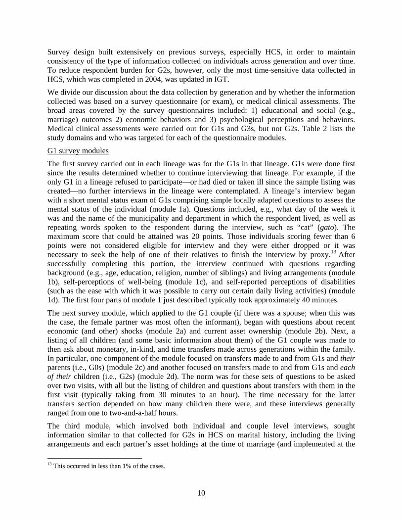
Survey design built extensively on previous surveys, especially HCS, in order to maintain consistency of the type of information collected on individuals across generation and over time. To reduce respondent burden for G2s, however, only the most time-sensitive data collected in HCS, which was completed in 2004, was updated in IGT.

We divide our discussion about the data collection by generation and by whether the information collected was based on a survey questionnaire (or exam), or medical clinical assessments. The broad areas covered by the survey questionnaires included: 1) educational and social (e.g., marriage) outcomes 2) economic behaviors and 3) psychological perceptions and behaviors. Medical clinical assessments were carried out for G1s and G3s, but not G2s. Table 2 lists the study domains and who was targeted for each of the questionnaire modules.

G1 survey modules

The first survey carried out in each lineage was for the G1s in that lineage. G1s were done first since the results determined whether to continue interviewing that lineage. For example, if the only G1 in a lineage refused to participate—or had died or taken ill since the sample listing was created—no further interviews in the lineage were contemplated. A lineage’s interview began with a short mental status exam of G1s comprising simple locally adapted questions to assess the mental status of the individual (module 1a). Questions included, e.g., what day of the week it was and the name of the municipality and department in which the respondent lived, as well as repeating words spoken to the respondent during the interview, such as “cat” (gato). The maximum score that could be attained was 20 points. Those individuals scoring fewer than 6 points were not considered eligible for interview and they were either dropped or it was necessary to seek the help of one of their relatives to finish the interview by proxy.13 After successfully completing this portion, the interview continued with questions regarding background (e.g., age, education, religion, number of siblings) and living arrangements (module 1b), self-perceptions of well-being (module 1c), and self-reported perceptions of disabilities (such as the ease with which it was possible to carry out certain daily living activities) (module 1d). The first four parts of module 1 just described typically took approximately 40 minutes.

The next survey module, which applied to the G1 couple (if there was a spouse; when this was the case, the female partner was most often the informant), began with questions about recent economic (and other) shocks (module 2a) and current asset ownership (module 2b). Next, a listing of all children (and some basic information about them) of the G1 couple was made to then ask about monetary, in-kind, and time transfers made across generations within the family. In particular, one component of the module focused on transfers made to and from G1s and their parents (i.e., G0s) (module 2c) and another focused on transfers made to and from G1s and each of their children (i.e., G2s) (module 2d). The norm was for these sets of questions to be asked over two visits, with all but the listing of children and questions about transfers with them in the first visit (typically taking from 30 minutes to an hour). The time necessary for the latter transfers section depended on how many children there were, and these interviews generally ranged from one to two-and-a-half hours.

The third module, which involved both individual and couple level interviews, sought information similar to that collected for G2s in HCS on marital history, including the living arrangements and each partner’s asset holdings at the time of marriage (and implemented at the

13 This occurred in less than 1% of the cases.

11

couple level, module 3a, see Quisumbing et al. 2005), and income generation and work history implemented at the individual level, while allowing for possible joint activities within the couple, for example in agriculture or small businesses (modules 3b and 3c). The survey instrument consisted of a four part questionnaire. Topics covered for the previous year included: 1) wage labor activities (type of work; hours, days, and months worked; wages and fringe benefits received; and a description of the employer); 2) agricultural activities (amount of land cultivated; crops grown; production levels; use of inputs; hours, days, and months worked); and 3) non-agricultural own-business activities (type of activity; value of goods or services provided; capital stock held; hours, days, and months worked). In addition, a brief work history was taken, with emphasis on what the individual was doing at age 50. These interviews typically ran from about 30 minutes to one hour (the questionnaires are described in further detail in Hoddinott, Behrman, and Martorell 2005).

The final G1 survey interview (apart from the clinical medical assessments described below) was a food frequency interview developed for this population and used previously in the Follow-up Study and HCS (Rodriguez et al. 2002; Stein et al. 2005) (module 4b). Respondents were asked to report how often they consumed a given food (from a list of over 60 foods commonly eaten in Guatemala) in terms of occasions per day, week, month, or year, and how many servings they consumed per occasion. The reference period for reporting was the past three months, and the survey took on average 30 minutes. To estimate energy and nutrient intakes, total consumption of each food item is determined by multiplying servings per day by the weight of a standard serving size (as ascertained in previous studies using 24-hour dietary recalls in this population). Total energy and nutrient intakes are then determined using the caloric and nutrient values for each food item as provided in the INCAP nutrient composition database (Menchu et al. 1996).

G1 clinical modules

There were three main components to the clinical medical assessment for G1s. The first was blood pressure, measured according to standard procedures during the initial contact with the individual (IPSLH 2003) (module 1e). Participants were instructed to refrain from use of tobacco products, alcohol, or caffeine in the 30 minutes preceding measurement. They then were to sit quietly with the left arm resting on a flat surface (at the level of the heart), for at least five minutes before the first measurement. Three separate measurements were taken at intervals of at least three minutes apart, with a digital sphygmomanometer (OMRON model UA-767, A&D Medical, Milpitas, CA) that was checked periodically for precision.

The second component was the medical history and physical exam (module 4a). A structured questionnaire was developed to obtain detailed information about medical history including personal and family history of health (e.g., chronic disease, surgeries, and trauma) (Ramírez-Zea et al. 2005). For women, a reproductive history that included the date of the last menstrual period, number of pregnancies and parity, smoking, drinking, medication, and drug consumption histories during pregnancies, and current symptoms of disease was taken (Ramakrishnan et al. 2005). For both men and women, the physician then conducted a standardized physical examination including body temperature, heart and respiratory rates, eyes, auditory channel, neck, thorax, back, abdomen, and limbs. Abnormalities and diagnoses of diseases were recorded. Subjects were informed of the results, offered medical advice, and referred to the Guatemalan health system when warranted.

12

The next part of the clinical assessment was anthropometric measurement. G1s were measured on body weight (kg), height (cm), and abdominal circumference (cm). They were weighed using a digital scale (model 1582, Tanita®, Japan) with a precision of 100 grams. Height was measured to the nearest 0.1 cm, with the subject bare foot, standing with their back to a stadiometer (GPM, Switzerland). Abdominal circumference was measured at the umbilicus using a plastic inextensible measuring tape to the nearest 0.1 cm. G1s were measured using standard methods (Lohman, Roche, and Martorell 1991). All measurements were done twice. If the difference between the two first measurements was greater than expected a third measurement was done and the two closest measurements were used. The mean of each measure was calculated.

In addition, the clinical assessment evaluated physical fitness via two tests: muscular strength and flexibility (Ramírez-Zea et al. 2005). Muscular strength was assessed using an isometric handgrip strength test. Handgrip strength correlates with total strength of 22 other muscles of the body (de Vries 1980). The test was performed using a Lafayette dynamometer (Model 78010, Lafayette Instrument Co., Lafayette, IN), with the subject in the standing position, the subject’s forearm at any angle between 90° and 180° of the upper arm, and wrist and forearm at the mid-prone position. All subjects were asked to exert a maximal and quick handgrip (Montoye and Lamphiear 1977).

The sit-and-reach test was used to assess flexibility of the hamstrings, lower back, buttocks, and calf muscles, according to the method of AAHPERD (1980). The test apparatus was a wooden box with a measuring scale (cm) on its upper surface. The technician asked each subject to remove their shoes, then sit on the floor with their feet against the box, keeping their legs fully extended, and feet about shoulder width apart. The technician held one hand on the subject’s knees while the participant bent forward as much as she or he could, with arms extended and hands placed on top of each other. Four trials were allowed and the maximal value was registered in cm.

The third component of the clinical assessment was blood testing (module 4c) (Ramírez-Zea et al. 2005). Whole blood samples were obtained by finger prick for blood glucose concentration and lipids concentrations after an overnight fast. Plasma glucose and lipid profile were determined with an enzymatic/peroxidase dry chemistry method (Cholestech LDX System, Hayward, CA). Lipid values were calibrated against a venous blood assay at Emory University’s Lipid Research Laboratory (Flores et al. 1998). LDL cholesterol concentration was calculated using Friedewald’s

equation (NCHE 2002). And lastly, hemoglobin concentration was measured using a portable photometer (Hemocue ABTM, Angelholm, Sweden).

G2 survey modules

The first several interviews with G2s focused on collecting information parallel or complementary to that collected for their G1 parents. These included information on economic and other shocks (module 5a), and current ownership of assets (module 5b). In addition, information on marital status (module 6a) and income generating activities (module 6b) were collected to update the information available from HCS (see criterion A1). Next, just as G1s were asked about transfers to and from their G2 children, each G2 was also asked about transfers to and from his or her G1 parents (module 5c). While for a variety of reasons these “cross” reports were not identical, they were largely consistent, and preliminary investigation indicates that these data correspond well to the data on transfers collected from G1s. The modules

13

typically took about one hour for women (who usually answered the couple-level questions regarding marital status, for example) and between 30 minutes and one hour for men. Risk assessment surveys, posing hypothetical “lottery” type comparisons were also carried out with G2s (module 6d).

The other main area for G2 survey interviews comprised the psychology component of the study, which focused attention on G2s as caregivers, including their interactions with their G3 children. We used three standardized questionnaires adapted to the local context, one to assess the level of stress related to caring for a young child, and two others to assess the level of psychological resilience of the mother and of the family.

A locally adapted version of the Parental Stress Index (PSI) (module 7b) short version was applied (Abidin 1995). The PSI identifies sources of stress in parent-child subsystems in three areas: 1) the child domain (e.g., child’s adaptability, mood); 2) the parent domain (e.g., role-related competence); and 3) the life stress domain (Abidin 1995). Mothers were asked how much they agreed or disagreed with statements regarding their children’s behavior and their parenting experiences, as well as several questions assessing their own emotional well-being. The PSI was designed for use with parents of children ranging in age from 1 month to 12 years. It has been adapted for use in Latin American Hispanic populations (Solis and Abidin 1991) and was extensively piloted and adapted further for use in this population. The mother was interviewed about her two youngest children between 1 and 11 years of age, with a separate interview per child, with interviews typically lasting about 20 minutes.

Two additional questionnaires were administered to the G2 mothers to assess the level of resilience of the mother (module 8a, Wagnild and Young 1993) and of the family (module 8b, McCubbin, McCubbin, and Thompson 1991). The information collected is used to evaluate how the mother and the family handle stressful situations in daily life, and perceptions on the level of control over their life situations and the cohesiveness of the family. Examples of questions assessing individual resilience include whether mothers feel they can follow through on plans that they make, whether believing in oneself helps during difficult times, and whether they are able to view situations from a variety of perspectives. Questions assessing family resilience focused on the family’s ability to work together, even during times of stress, the family feeling valued, and whether they are able to overcome and survive difficult times.

All three surveys were adapted into Spanish for this population, back-translated into English for verification, and piloted extensively in a community similar to the study communities. Interviewers were given extensive training in the phrasing and implementation of the questions, and in ethical issues relevant to administering these types of questionnaires. In order to assure that women understood the questions correctly, several procedures were implemented. First, interviewers asked the mother to respond to three questions as an example of the types of questions on the questionnaire to verify that she understood the instructions. Second, for the first five questions, the interviewer re-read each question together with the response given from the mother, verifying that the response reflected the true thinking of the mother for each question. For illiterate mothers, the administration was similar except the interviewer read aloud the five response options for each question on the questionnaires (in contrast to assuming the respondent remembered them or could read them from the visual aids).

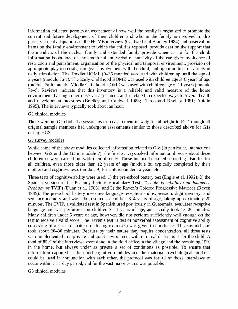
Mothers or main child caretakers also were interviewed regarding the youngest child at home to assess the potential for physical, intellectual, and social-emotional stimulation for that child. The

14

information collected permits an assessment of how well the family is organized to promote the current and future development of their children and who in the family is involved in this process. Local adaptations of the HOME interview (Caldwell and Bradley 1984) and observation items on the family environment to which the child is exposed, provide data on the support that the members of the nuclear family and extended family provide when caring for the child. Information is obtained on the emotional and verbal responsivity of the caregiver, avoidance of restriction and punishment, organization of the physical and temporal environment, provision of appropriate play materials, caregiver involvement with the child, and opportunities for variety in daily stimulation. The Toddler HOME (0–36 months) was used with children up until the age of 3 years (module 7a-a). The Early Childhood HOME was used with children age 3–6 years of age (module 7a-b) and the Middle Childhood HOME was used with children age 6–11 years (module 7a-c). Reviews indicate that this inventory is a reliable and valid measure of the home environment, has high inter-observer agreement, and is related in expected ways to several health and development measures (Bradley and Caldwell 1988; Elardo and Bradley 1981; Abidin 1995). The interviews typically took about an hour.

G2 clinical modules

There were no G2 clinical assessments or measurement of weight and height in IGT, though all original sample members had undergone assessments similar to those described above for G1s during HCS.

G3 survey modules

While some of the above modules collected information related to G3s (in particular, interactions between G2s and the G3 in module 7), the final surveys asked information directly about these children or were carried out with them directly. These included detailed schooling histories for all children, even those older than 12 years of age (module 8c, typically completed by their mother) and cognitive tests (module 9) for children under 12 years old.

Three tests of cognitive ability were used: 1) the pre-school battery test (Engle et al. 1992); 2) the Spanish version of the Peabody Picture Vocabulary Test (Test de Vocabulario en Imagenes Peabody or TVIP) (Dunn et al. 1986); and 3) the Raven’s Colored Progressive Matrices (Raven 1989). The pre-school battery measures language reception and expression, digit memory, and sentence memory and was administered to children 3–4 years of age, taking approximately 20 minutes. The TVIP, a validated test in Spanish used previously in Guatemala, evaluates receptive language and was performed on children 3–11 years of age, and usually took 15–20 minutes. Many children under 5 years of age, however, did not perform sufficiently well enough on the test to receive a valid score. The Raven’s test (a test of nonverbal assessment of cognitive ability consisting of a series of pattern matching exercises) was given to children 5–11 years old, and took about 20–30 minutes. Because by their nature they require concentration, all three tests were implemented in a private and quiet environment with minimal distractions for the child. A total of 85% of the interviews were done in the field office in the village and the remaining 15% in the home, but always under as private a set of conditions as possible. To ensure that information captured in the child cognitive modules and the maternal psychological modules could be used in conjunction with each other, the protocol was for all of those interviews to occur within a 15-day period, and for the vast majority this was possible.

G3 clinical modules

15

In addition to these cognitive tests, all children under 12 years old were given a medical clinical history (module 10a) and anthropometric measures were taken (module 10b). The clinical evaluation of G3s included a medical history comprising fetal, delivery, early feeding, and immunization histories, and a comprehensive physical exam. The physical assessment used the same equipment as used for the G3s, but age appropriate techniques for children. Weight (kg), was taken using a digital scale (model 1582, Tanita®, Japan) appropriate for measuring both adults and small children, with a precision of 100 grams. Cephalic arm, abdomen and calf circumferences (cm) were measured using a plastic inextensible measuring tape to the nearest 0.1 cm. Triceps and sub scapular skin folds (mm) were measured using a Holtain skinfold caliper. Height was measured to the nearest 0.1 cm, with the subject bare foot and standing with their back to a stadiometer (GPM, Switzerland), for children up to 36 months of age. Length was measured to the nearest 0.1 cm using a wood stadiometer for children under 36 months of age.

2.5.3 Interviewer training and quality control

Before the data collection phase, one physician, two field supervisors and four experienced interviewers, all familiar with the original study villages and having worked on HCS were hired. In addition, five new field workers were recruited to be trained alongside the more experienced ones, and three teams were formed. The first team was responsible for the “interview” modules carried out with G1 and G2 sample members (modules 1, 2, and 3 for G1s and modules 5 and 6 for G2s). The second team, comprising a physician and one interviewer, both trained in anthropometry, food frequency surveys, and how to take blood samples, was responsible for the clinical and physical assessments of G1s and G3s (module 4 for G1s and module 10 for G3s). Finally, the third team was responsible for the psychological modules carried out with G2s and G3s. Two interviewers were trained to administer the interview-observations with mothers of G3s (modules 7 and 8). The other two interviewers on this team were trained to administer the G3 cognitive tests (module 9).

Code books were prepared for each form, questionnaire, or test. Each team of interviewers was trained in interviewing techniques and interpretations were standardized using the manuals designed for each module (and according to their assigned team). During the fieldwork, supervisors and coordinators accompanied interviewers weekly to monitor the interview quality, both carrying out duplicate interviews and filling out forms simultaneously during a regular interview. Immediately after all interviews, 100% of the forms were reviewed by the enumerator who would return to re-interview the respondent if she found any errors. Supervisors also reviewed approximately 15% of all forms (arbitrarily selected). When errors were found, corrections were made in the office if possible but if not, the original interviewer would return to re-collect the data in question from the respondent. In addition, there were periodic re-standardizations (including directed readings of the manuals for each module and practice, as well as observation in the field by supervisors). When comparisons were made after the interview, agreement was consistently above 95%.

Fieldwork was made difficult by the complicated structure of the various surveys as well as by the need to accommodate respondents’ schedules, particularly men working in wage labor. Strategies to contact these subjects included scheduling afternoon, evening, and weekend interviews. In general, interviews were ordinarily spread over time and on multiple visits to avoid overburdening respondents (but keeping within a three-month period), and were scheduled at times convenient to respondents and were carried out in respondent’s homes (with the

16

exceptions noted above). In Guatemala City, data collection difficulties were magnified by the dispersion of the sample members all around the city.

2.5.4 Data management

Double-data entry was carried out in the field headquarters using Microsoft Access 2003 and Microsoft Visual Basic for Applications. The data entry programs directly incorporated range and consistency checks. In general, data were entered within one week of collection. Data entry errors were about 2% of the total data entered, all of which were corrected after being identified by comparing the double-entered data.

The second data cleaning phase consisted of implementing verification routines written in Stata 9.0, and run on a monthly basis; these programs included range checks and logical consistency checks that could not be directly incorporated into Microsoft Access, both within and between modules. Questionnaires with range check or logical consistency errors were returned to the field to be corrected by the original interviewer, after which they had to be approved by the supervisor. This system allowed interviewers to revisit respondents shortly after the original interview to facilitate re-interviewing and to keep reference periods consistent.

For the anthropometry and clinical history forms, a pilot test was carried out using pocket PCs (all other interviews used paper forms). These offered a potentially substantial gain in efficiency since pretests suggested it was straightforward to capture and download the data from the Pocket PC to the desktop computers used for data entry. The same information also was collected using the usual paper forms and data entry protocols. After three months of piloting, the pocket PCs had a 4% error rate for the medical history module (with 178 questions) and a 2% error rate for the anthropometry module (with 43 questions), treating the paper forms as being correct. Two additional problems with using pocket PCs were that they required special care in dusty environments (particularly rural areas) and they likely increased the risk of enumerators being targeted for crime in insecure environments (particularly in urban areas). For all these reasons, thus use of pocket PCs was suspended for the remainder of the fieldwork.

3. Results

3.1 Target sample and coverage

Using the criteria outlined in Section 2.1, we now characterize the target sample for original sample members and for their extended family members in the lineages. Eligibility as original sample members was determined using criteria A1–A3. There were 1,033 (43% of original 2,392) individuals satisfying all three criteria (Table 3). For those that did not, 383 (16%) had died by the time of the IGT survey (most during early childhood) and 624 (26%) were living outside the IGT study area or could not be traced. The remaining 352 (15%) individuals were ineligible either because they had not completed the relevant forms for HCS, they did not have an eligible G1 parent living in the IGT study area, or both.

In addition to these 1,033 original sample members eligible based on A1–A3, when we consider eligibility for the sample based on extended family connections under criteria B1–B3, 57 additional original sample members became eligible, as while ineligible as original sample members on their own account, they were married to eligible original sample members (B2). Thus, the total number of eligible original sample members for the study is 1,090 (46% of original sample and 54% of those alive in 2007).

17

In Table 4, we show by generation and sex all the eligible parents (G1), spouses (G2), and children (G3) of those 1,090 (496 males and 594 females) eligible original sample members. The final target sample included 756 G1s, 1,090 original sample member G2s, 505 G2 spouses, and 1,463 G3s, for a total of 3,814 individuals. There were about 150 more women than men, and this imbalance was concentrated in the G1 and original sample member G2 categories, consistent with longer life-spans for women and higher probabilities of finding and interviewing G2 original sample women compared with men, who were more likely to migrate.

The 3,814 individuals (1,828 males and 1,986 females) were spread across 452 lineages, where it is possible that individuals are in more than one lineage as a result of marriage between original sample members. Lineages ranged from 2 to 30 members and averaged 9.5 individuals. Each lineage has an average 1.7 G1s, 4.0 G2s, and 3.8 G3s. About one-third had a single G1 (and three-quarters of these were women), with nearly all the rest having two G1s forming a couple. The number of original sample member G2s within a lineage ranged from 1 to 8, though most had between 1 and 4 members. There was an average of 1.7 G2s per lineage that were not original sample members (but were spouses of eligible original sample members entering via criterion B2). Approximately 12% of the lineages had no G3s.

Table 4 shows the percentage in each generation that (wholly or partially) completed the survey. 78% of all sample members completed all the survey modules, and an additional 16% completed some of the modules, leaving only 6% who did not complete any interviews. Complete or partial interviews were highest for G1s and G3s compared with G2s, who had failure rates of 6–9%. Partial interviews were most common for G1s. Coverage rates for G1s who completed all modules except the blood test, however, are substantially higher than those for complete coverage, at 73% (versus 565) for men and 85% (versus 76%) for women, as shown in italics. Consequently there are similar, though much smaller (2–3 percentage point) increases in total coverage when we consider this measure without blood tests. Finally, while G1 and G2 men had about the same overall coverage as G1 and G2 women, men were much more likely to have only partially completed sets of interviews (for G1s, 38% of men had partial interviews compared with 19% for women; for G2 original sample members, 17% versus 6%; and for G2 spouses, i.e., those who had not participated in the INCAP Longitudinal Study, 14% versus 3%). This pattern is similar, though less pronounced, when we consider the complete except for blood test measure.

In Table 5, we present coverage of the different questionnaire modules described in Section 2.5.2. Different modules were applicable at the G1, G2, and G3 generational levels, and in some cases were applicable to different sets of persons within those levels. We indicate for each module the target sample in the left-hand-side column and then the number of completed interviews and coverage rate (separating out men and women, where relevant). For women and men combined, all but two of the modules have coverage of 86% or higher (and for G3s, all but one had coverage 90% or above). The exceptions include blood tests for G1s (71%) and the marriage, income, and work history for G2s (82%). For all G1 and G2 interviews, coverage for men was lower than for women, and by as much as 20 percentage points for the blood tests (60% versus 80%). Coverage was about equal in the origin communities and the remainder of El Progreso, but generally lower in Guatemala City. This latter pattern was particularly true for males in Guatemala City, who proved the most difficult to interview, often because of their work schedules.

Attrition

18

The discussion of coverage demonstrates how successful the study was in interviewing those in the target sample, the result of the various methodologies for tracing that were in place. Because not all original sample members were targeted, even if 100% of the target sample had been interviewed, however, the study would still have had substantial attrition, defined as original sample members who were not interviewed in 2006–07. When making inference about the population using these data, what is most relevant to the analyst is not necessarily the coverage of the target sample, but rather overall attrition. What are the characteristics of individuals not interviewed, for whatever reason, in 2006–07?

Because we cannot know the composition of the extended families (spouses and children) of those individuals we did not contact during the fieldwork, it is not possible for us to determine the set of potential interviews for the entire survey, against which we could compare the target list and those actually interviewed in a standard attrition analysis. Instead, then, we focus attention on the two subpopulations we do have complete information on—original sample member G2s and their G1 parents. Our maintained hypothesis is that patterns for these groups will provide general a general indication of the underlying attrition biases for the entire sample.

We use multinomial logistic regression to describe the factors associated with attrition, with the outcome variable defined as eligible and interviewed (the base category), eligible but not interviewed, ineligible (for a reason other than death), and deceased. Using this framework, we analyze attrition for G2 original sample members and then, separately, G1s.

First, we explore whether average characteristics of G2s vary across the different categories (Table 6). In total, 1,009 original sample members (42% of all original sample members, 50% of surviving original sample members, and 93% of the targeted original sample members) were interviewed (at least partially), while 81 (3% of all 2,392) eligible original sample members were not interviewed, 919 (39%) were ineligible, and the remaining 383 (16%) were deceased. While about two-thirds of the variables show significant differences across categories using an analysis of variance (ANOVA) test (second to last column), fewer than half show significant differences when we compare means between the interviewed and all non-interviewed (for any reason) individuals together, using two sample t-tests or proportion tests as appropriate (final column). In many of the cases where there are significant differences based on the ANOVA tests, they are in opposite directions across categories within the not-interviewed group such that on average the group not interviewed is not significantly different from the group that was interviewed. This suggests that, while not random, the average differences across attrition groups are not substantial. Further, for those that do differ by either test, several do not appear to be very large differences. For example, the year of birth varies by only 1.2 years, the proportion born in Espíritu Santo by only 7 percentage points, the SES score by less than 0.3 standard deviations (SD), and the height-for-age z-score at 2 years of age by less than 0.2 SD. On the other hand, mothers’ schooling varies by more than 0.5 grades (in a population with less than 2 years on average) and the fraction of males by 12 percentage points. Assessing the missing dummy variable for SES scores (or for height-for-age z-scores measured at 24 months of age), we also see disproportionately missing information for those either ineligible or deceased.

In Table 7, we use a multinomial logit to explore the associations between the characteristics in Table 6 (apart from the childhood height-for-age z-score measure) and attrition. Attrition in the sample is largely unassociated with the initial conditions considered, though there are some exceptions. In particular, men were substantially more likely to be eligible but not interviewed, ineligible (usually due to migration outside of the eligible study areas, e.g., internationally), or

19

deceased, relative to being interviewed. In each case, the odds-ratios across these different categories were similar. The association of later birth year with being less likely to be ineligible (relative to being eligible and interviewed) is consistent with older individuals being more likely to be out of the sample, for example having migrated to other areas. The association of later year of birth, i.e., younger age, with risk of death is somewhat counterintuitive, but results from the inclusion in the original sample of all children less than seven years in 1969. These represent the survivors of their respective birth cohorts, and hence they experienced a lower mortality rate (most of which is driven by infant mortality) compared with the later birth cohorts in the study who were followed from birth. Individuals born in Espíritu Santo were less likely to be eligible but not interviewed compared with Santo Domingo; this is consistent with somewhat higher cooperation with the study team in Espíritu Santo. Also, we can explore in this table whether there is a difference with respect to atole villages, since the San Juan and Conacaste indicator dummy variables add to an atole indicator. For the ineligible and deceased categories, the two village level indicators are both insignificant and yield odds ratios on both sides of one, suggesting there is no significant effect of atole. This turns out also to be the case for the eligible category when we combine the two indicators (results not shown). Individuals with missing information about their parents or past wealth were generally more likely to be ineligible, reflecting a subset of individuals who were untraceable in HCS or IGT and, in all probability, left the villages during the 1970s and have not been located since.

We next consider attrition at the level of G1, which more closely corresponds to what we might consider attrition at the “lineage” level. While this analysis is possible because we have information on the universe of possible G1s, it is less rich than for the original sample member G2s because we have less information about them. Using the same categories for types of attrition, however, we again look at the mean characteristics across groups and then estimate a multinomial logit.

There are significant differences across nearly all the categories based on an ANOVA test (second to last column, Table 8), but only about half based on two sample t-tests or proportion tests as appropriate (final column). As was the case for G1s, many variables have both higher and lower averages in the subcategories when compared to those who were successfully interviewed in IGT. Major differences, however, include the higher proportion of men and earlier year of birth in the deceased category, and the lower average number of children in the deceased and ineligible categories. Schooling levels were also much lower in the deceased category (as well as nearly one-third a grade lower for those interviewed compared to those not interviewed or ineligible). Finally, as with G2s, larger proportions of ineligible or deceased are missing information from the early census rounds on their wealth levels.

Examining the results from the multinomial logit (Table 9), G1 men were substantially more likely to be deceased (relative to being interviewed), consistent with their on average older age and higher probability of death than their partners. In contrast, individuals born later (i.e., younger G1s) or who had had children later, as well as with more formal schooling, were less likely to be deceased relative to those eligible and interviewed. The number of children is associated with lower likelihood of being ineligible (probably because in this way it was more likely to have a G2 who was eligible) and also a lower likelihood of being deceased. There are also some significant patterns with respect to village of origin, with the main results that villagers in atole villages and in Espíritu Santo were less likely to have been eligible but not interviewed or ineligible, but more likely to have been deceased, compared with Santo Domingo. Since G1s

20

were already adults during the intervention, it seems unlikely that these are effects of the intervention itself; they more likely reflect differential patterns by village, perhaps associated with proximity to Guatemala City.

This analysis, while descriptive, underscores that attrition in the sample is not random, though it is reassuring that for G2s, who were children during the intervention, attrition does not appear to be related to the original intervention. Analysts will need to consider the potential effects of attrition when using these data and, to mitigate them may want to control for some of these initial factors.

4. Conclusions In this paper, we have introduced the Resource Flows Among Three Generations in Guatemala Study, or IGT, carried out in 2006–07. In doing so, we provide a guide for using and interpreting the data collected as part of IGT, as well as an example for others interested in implementing research projects on similar themes elsewhere.

The aim of the survey was to provide information to examine the allocation of resources across generations, and the consequences of those allocations, in a developing country. The micro-empirical investigation of these issues imposes immense data requirements and, consequently, data collection challenges. In this paper, we described how we met those challenges, building on a well-known study from Guatemala.

Relatively complicated research topics, across generations and across a range of possible measures of well-being, led to a relatively complicated sample selection process and survey design, with component modules that were applicable to different “types” of sample members, depending on their age and generational status. It also led to a wide variety of survey domains, including economic, educational, and psychological surveys to clinical medical exams for both the young and the elderly. Often, sample members in the same extended family lived in different locations, increasing the logistical difficulties of the study.

Survey coverage was above 85% of the targeted sample for most categories of respondents and most modules, and a number of safeguards were in place to ensure high quality data, even before extensive cleaning routines were implemented. Biases due to attrition, measured against the original 1970s rounds of survey work, while present, should not reduce substantially the validity of research findings to come from this rich sample. The extent to which this is true, though, may vary depending on the topic under consideration and the controls included in the analyses.

21

References Abidin, R. 1995. Parenting Stress Index, Third Edition. Professional Manual. Odessa, FL:

Psychological Assessment Resources, Inc.

American Alliance for Health, Physical Education, Recreation, and Dance (AAHPERD). 1980. AAHPERD health related physical fitness test. Reston, VA: AHHPERD.

Behrman, J, S. Duryea and M. Székely. 2003. Aging and economic opportunities: Major world regions around the turn of the century, in O. Attanasio and M. Székely (eds.) A Dynamic Analysis of Household Decision-Making in Latin America. Washington, DC: Inter-American Development Bank.

Behrman, J, S. Duryea and J.A. Maluccio. 2008. Addressing early childhood deficits in Guatemala, Washington, DC: Inter-American Development Bank. Photocopy.

Bradley R.H., and B.M. Caldwell. 1988. Using the HOME Inventory to assess the family environment, Pediatric Nursing 14: 97–102.

Caldwell B.M., and R.H. Bradley. 1984. Administration Manual, Revised Edition, Home Observation for Measurement of the Environment. Little Rock, AK: University of Arkansas.

Dunn, Lloyd M, E.R. Padilla, D.E. Lugo and Leota M. Dunn. 1986. Peabody Picture Vocabulary Test: Hispanic-American Adaptation, Circle Pines, Minnesota: American Guidance Service.

Elardo, R., and R.H. Bradley. 1981. The Home Observation for Measurement of the Environment (HOME) Scale: A review of research, Developmental Review 1(2): 113–45.

Engle, P.L., K. Gorman, R. Martorell, and E. Pollitt. 1992. Infant and pre-school psychological development, Food and Nutrition Bulletin 14 (3): 201–14.

Flores R., R. Grajeda, B. Torun, H. Mendez, R. Martorell, and D. Schroeder. 1998. Evaluation of a dry chemistry method for blood lipids in field studies, FASEB Journal 12: S3061(abs.).

Grajeda, R., J.R. Behrman, R. Flores, J.A. Maluccio, R. Martorell, and A.D. Stein. 2005. The Human Capital Study 2002–04: Research design and implementation of the early nutrition, human capital, and economic productivity study, Food and Nutrition Bulletin, 26(2) (Supplement 1): S15–S24.

Habicht, J.-P., and R. Martorell. 1992. Objectives, research design, and implementation of the INCAP longitudinal study, Food and Nutrition Bulletin 14 (3): 176–90.

Hoddinott, J., J.R. Behrman, and R. Martorell. 2005. Labor force activities and income among young Guatemalan adults, Food and Nutrition Bulletin 26 (2) (Supplement 1): S98–S109.

Iniciativa Panamericana Sobre La Hipertensión (IPSLH). 2003. Working meeting on blood pressure measurement: suggestions for measuring blood pressure to use in populations surveys, Revista Panamericana Salud Publica 14: 300–5.

Lohman, T.G., A.F. Roche, and R. Martorell (eds.). 1991. Anthropometric Standardization Reference Manual. Champaign, IL: Human Kinetics.

22

Martorell, R., J.R. Behrman, R. Flores, and A.D. Stein. 2005. Rationale for a follow-up study focusing on economic productivity, Food and Nutrition Bulletin, 26(2) (Supplement 1): S5–S14.

Martorell, R., J-P. Habicht, and J.A. Rivera. 1995. History and design of the INCAP longitudinal study (1969–77) and its follow-up (1988–89), Journal of Nutrition, 125(4S): 1027S–41S.

McCubbin, M.A., H.I. McCubbin, and A. Thompson. 1991. Family Hardiness Index (FHI): Family Assessment Inventories for Research and Practice, Madison, WI: University of Wisconsin-Madison.

McNiven, S. 2008. The February 2008 IGT data release. International Food Policy Research Institute, Washington D.C. Photocopy.

Melgar, P., and L.F. Ramírez. 2008. Manual de Operaciones: Resource Flows Among Three Generations in Guatemala Study. Guatemala City, Guatemala: INCAP (in Spanish).

Menchu, M.T., H. Méndez, M.A. Barrera, and L. Ortega. 1996. Nutritional value of Central American foods. Guatemala City, Guatemala: INCAP (in Spanish).

Montoye H.J., and D.E. Lamphiear. 1977. Grip and arm strength in males and females, age 10 to 69, Research Quarterly (48): 109–20.

National Cholesterol Education Program (NCHE). 2002. Third Report of the expert panel on detection, evaluation, and treatment of high blood cholesterol in adults. NIH Pub. No. 02-5215. Bethesda, MD: National Heart, Lung, and Blood Institute.

Quisumbing, A.R., J.R. Behrman, J.A. Maluccio, A. Murphy, and K.M. Yount. 2005. Levels, correlates, and differences in human, physical, and financial assets brought to marriages by young Guatemalan adults, Food and Nutrition Bulletin, 26(2) (Supplement 1): S55–S67.

Ramakrishnan, U., K.M. Yount, J.R. Behrman, M. Graff, R. Grajeda, and A.D. Stein. 2005. Fertility behavior and reproductive outcomes among young Guatemalan adults, Food and Nutrition Bulletin, 26(2) (Supplement 1): S68–S77.

Ramírez-Zea, M., P. Melgar, R. Flores, J. Hoddinott, U. Ramakrishnan, and A.D. Stein. 2005. Physical fitness, body composition, blood pressure, and blood metabolic profile among young Guatemalan adults, Food and Nutrition Bulletin, 26(2) (Supplement 1): S88–S97.

Raven, J.C. 1989. Test de Matrices Progresivas Escala Coloreada. Adaptación Argentina. Argentina: J.C. Raven.

Read, M. S., and J.-P. Habicht. 1992. History of the INCAP longitudinal study on the effects of early nutrition supplementation in child growth and development. Food and Nutrition Bulletin 14 (3): 169–75.

Rodriguez, M.M., H. Méndez, B. Torún, D. Schroeder, and A.D. Stein. 2002. Validation of a semi-quantitative food frequency questionnaire for use among adults in Guatemala, Public Health Nutrition 5: 691–98.

Solis, M.L., and R.R. Abidin. 1991. The Spanish version of the Parenting Stress Index: A psychometric study, Journal of Clinical Child Psychology, 20: 372–8.

Stein, A.D., C.O. Gregory, J. Hoddinott, R. Martorell, U. Ramakrishnan, and M. Ramírez-Zea.

23

2005. Physical activity level, dietary habits, and alcohol and tobacco use among young Guatemalan adults, Food and Nutrition Bulletin, 26(2) (Supplement 1): S78–S87.

Stein, A.D., P. Melgar, J. Hoddinott, and R. Martorell. 2008. Cohort profile: The Institute of Nutrition of Central America and Panama (INCAP) nutrition trial cohort study. International Journal of Epidemiology (2008 Feb 19, published on-line).

de Tejada S., L. Mazariegos and L. Barrios. 2005. Intergenerational exchanges in four Guatemalan communities: Final report prepared for the International Food Policy Research Institute. Guatemala City, Guatemala: Estudio 1360.

United Nations. 2001. World Population Ageing 1950–2050. New York, NY: United Nations Population Division.

deVries, H.A. 1980. Physiology of exercise in physical education and athletics. Dubuque, IA: William C. Brown.

Wagnild G.M., and H.M. Young. 1993. Development and psychometric evaluation of the Resilience Scale, Journal of Nursing Measurement 1(2): 165–78.

24

Figure 1–Map of the original villages

25

Figure 2–Example of simplest possible lineage

Figure 3–Example of lineage in which G1 parents have remarried

Biological father (G1)

Eligible original sample

member (G2)

Biological mother (G1)

Biological father’s new spouse (G1)

Biological mother’s new spouse (G1)

Spouse (G2)

Eligible original sample

member (G2)

Biological child (G3)

Biological child (G3)

Adopted child (G3)

Biological parent (G1)

Eligible original sample member

(G2)

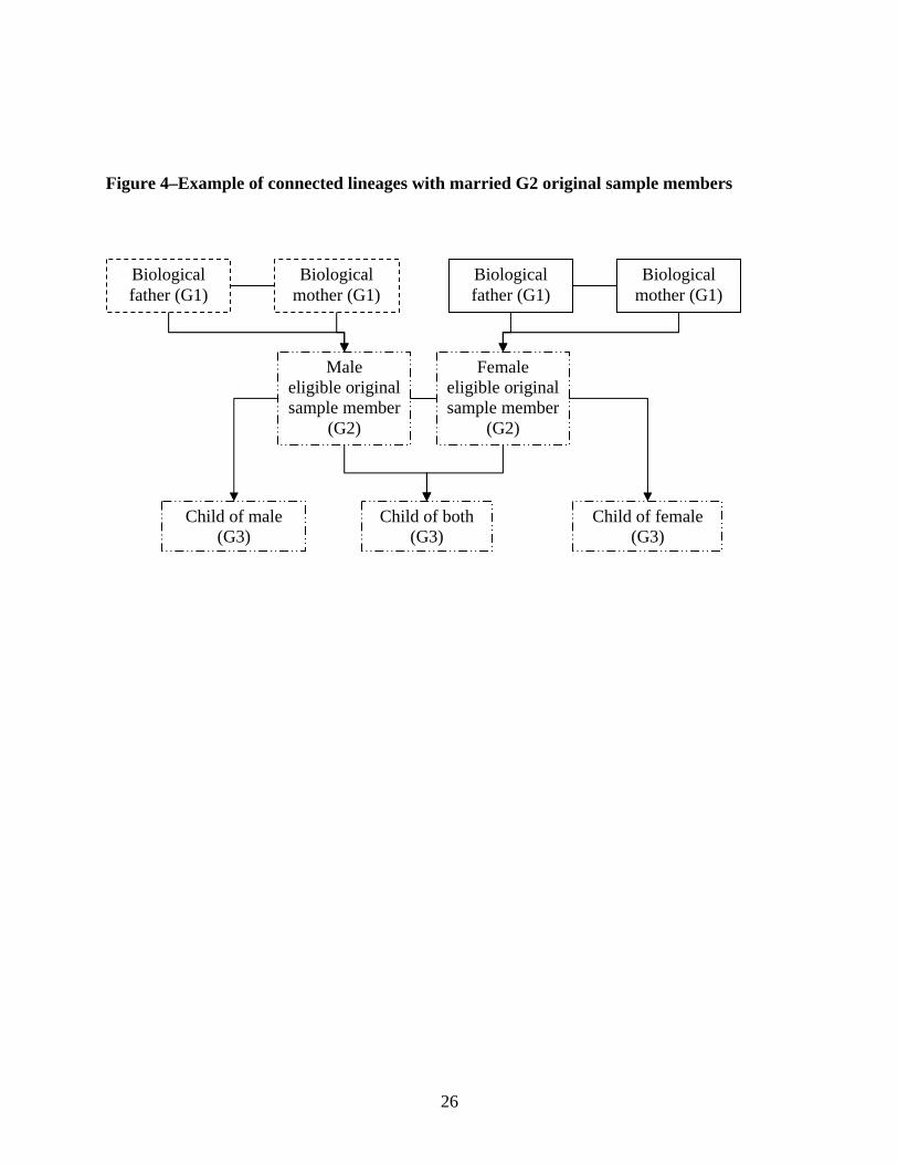
26

Figure 4–Example of connected lineages with married G2 original sample members

Biological father (G1)

Female eligible original sample member

(G2)

Biological mother (G1)

Male eligible original sample member

(G2)

Child of male (G3)

Child of both (G3)

Child of female (G3)

Biological father (G1)

Biological mother (G1)

27

Table 1–Chronogram of IGT activities

Trimester 2005 2006 2007 2008

Activity 2 3 1 2 3 1 2 3 1 2 3

Project promotion and community rapport

Questionnaire development and pilot testing

Update sample listing and lineages

Field team selection, training, refresher training

Data collection in original four villages

Data collection in nearby villages and Guatemala City

Data entry (including design)

Data validation and cleaning

Preparation of final project documentation

Report back to participants, community leaders, and health authorities

28

Table 2–Study domains and data collection for IGT Module Description Individual or couple

M1a M1b M1c M1d M1e

Mini mental status exam (MMSE) Background (education & residential arrangements) Self-perceived well-being Self-reported disability, activities of daily living Blood pressure

All G1 individuals

M2a M2b M2c M2d

Economic & other shocks Assets & housing characteristics G0 characteristics & transfers between G0 & G1 G2 characteristics & transfers between G1 & G2

All G1 couples

M3a-a, a-b Marriage History & Assets M3b-a Wage labor income

All G1 individuals

M3b-b&c Agricultural and business income All G1 couples M3c Work History All G1 individuals

G1s

M4a M4b M4c

Medical clinical history (including anthropometry) Food frequency Blood test

All G1 individuals

M5a M5b M5c

Economic & other shocks Assets & housing characteristics Transfers between G1 & G2

All G2 Couples

M6a-a, a-b Changes in marital status since HCS All G2 original sample members

M6ba M6d

Wage labor income Risk assessment All G2 individuals

M6b-b&c Agriculture and business income All G2 couples

M8a Individual resilience All G2 women

M8b Family resilience All G2 women with children or a spouse

G2s

M8c G3 Schooling History G2 couples with children M7a-a M7a-b M7a-c

HOME I HOME II HOME III

Youngest G3 ages 1–11 G3 age 1–3 G3 age 4–5 G3 age 6–11

M7b Parental Stress Index (PSI) Youngest two G3s ages 1–11 M9a M9b M9c

TVIP RAVEN Pre-school battery

G3s ages 3–11 G3s ages 5–11 G3s ages 3–4

G3s

M10a M10b

Medical clinical history Anthropometry All G3 children ages 1–11

29

Table 3–Eligibility of original sample members

Completed relevant HCS

forms (A1) Did not complete HCS

forms (not A1)

G1 parent living in

IGT study area (A3)

No G1 parent

living in IGT study

area (not A3)

G1 parent living in

IGT study area (A3)

No G1 parent

living in IGT study area (not

A3) TotalLiving in IGT study area (A2) 1033 81 259 12 1385of which spouse eligible 240 10 43 4 297

Dead 7 0 200 176 383Living outside IGT study area 83 124 188 229 624Total (excluding spouse eligible) 1123 205 647 417 2392Notes: 57 of original sample members are included in the study because while ineligible by A1–A3, they are spouses of eligible original sample members (B2) (shown in second row). Therefore, a total of 1090 original sample members were eligible.

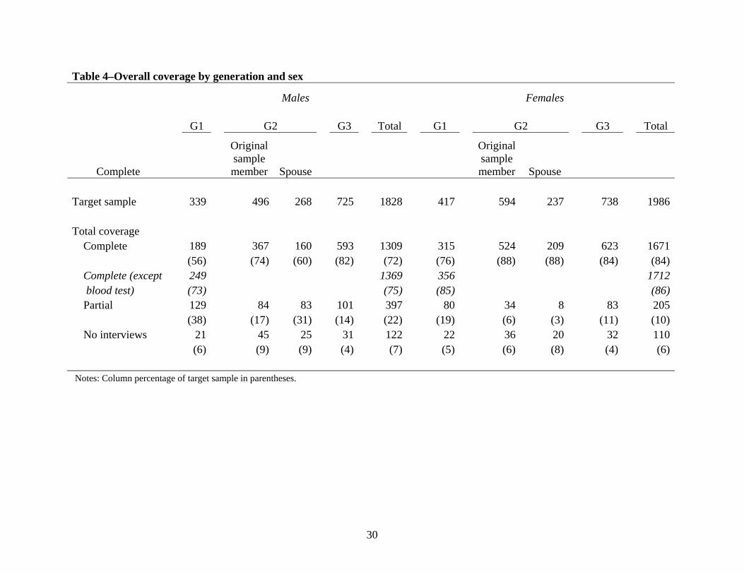
30

Table 4–Overall coverage by generation and sex

Males Females

G1 G2 G3 Total G1 G2 G3 Total

Complete

Original sample member Spouse

Original sample member Spouse

Target sample 339 496 268 725 1828 417 594 237 738 1986 Total coverage

Complete 189 367 160 593 1309 315 524 209 623 1671 (56) (74) (60) (82) (72) (76) (88) (88) (84) (84)Complete (except 249 1369 356 1712 blood test) (73) (75) (85) (86)Partial 129 84 83 101 397 80 34 8 83 205 (38) (17) (31) (14) (22) (19) (6) (3) (11) (10)No interviews 21 45 25 31 122 22 36 20 32 110

(6) (9) (9) (4) (7) (5) (6) (8) (4) (6) Notes: Column percentage of target sample in parentheses.

31

Table 5–Total subjects interviewed and percent of target sample

TotalOrigin

Community El ProgresoGuatemala

CityN (%) N (%) N (%) N (%)

G1 individuals (N=756)Men 289 (85) 260 (87) 16 (84) 13 (65)Women 387 (93) 342 (93) 22 (92) 23 (85)Total 676 (89) 602 (90) 38 (88) 36 (77)

Men 285 (84) 256 (85) 16 (84) 13 (65)Women 384 (92) 339 (93) 22 (92) 23 (85)Total 669 (88) 595 (89) 38 (88) 36 (77)Men 268 (79) 243 (81) 13 (68) 12 (60)Women 380 (91) 335 (92) 22 (92) 23 (85)Total 648 (86) 578 (87) 35 (81) 35 (74)Men 271 (80) 244 (81) 15 (79) 12 (60)Women 378 (91) 335 (92) 21 (88) 22 (81)Total 649 (86) 579 (87) 36 (84) 34 (72)

Men 205 (60) 185 (62) 9 (47) 11 (55)Women 334 (80) 296 (81) 18 (75) 20 (74)Total 539 (71) 481 (72) 27 (63) 31 (66)

G2 individuals (N=1,595)Men 547 (72) 400 (77) 62 (58) 85 (63)Women 763 (92) 528 (93) 94 (85) 141 (92)Total 1310 (82) 928 (85) 156 (72) 226 (78)

Original sample members (N=1090)Men 387 (78) 306 (80) 29 (66) 52 (74)Women 550 (93) 390 (94) 61 (81) 99 (94)Total 937 (86) 696 (87) 90 (76) 151 (86)

G1 Couples (N=479)Module 2abc : Shocks, assets, transfers to G0 435 (91) 385 (92) 23 (85) 27 (79)Module 2d : Registry of and transfers to children 436 (91) 386 (92) 23 (85) 27 (79)G2 Couples (N=900)Module 5 : Shocks, assets, transfers to G1 817 (91) 578 (92) 94 (82) 145 (92)G2 Women (N=833)Module 8a : Individual resilience 757 (91) 521 (92) 95 (86) 141 (92)G2 Women with children or a spouse (N=765)Module 8b : Family resilience 720 (94) 491 (95) 94 (90) 135 (96)G2 Couples with children (N=798)Module 8c : Schooling history of children of G2s 712 (89) 488 (90) 91 (83) 133 (90)Two youngest G3s between 1 and 11 years (N=1118)Module 7 : HOME and Parental Stress Index 1045 (93) 720 (93) 140 (94) 185 (95)G3s age 3-11 (N=1314)Module 9 : TVIP, RAVEN or Preschool Battery 1182 (90) 831 (90) 156 (88) 195 (90)G3s age 0-11 (N=1463)Module 10a : Pediatric clinical history 1369 (94) 970 (95) 177 (88) 222 (92)Module 10b : Pediatric anthropometry 1375 (94) 969 (95) 184 (91) 222 (92)Notes: Target sample for each category shown in bold; percent of target for each subcategory in parentheses.

Module 1 : MMSE, background, self-perceived well-being, self-reported disability, and blood pressure

Module 6a : Changes in marital status since 2002

Module 6 : Marriage history, income, work history, risk

Module 4c : Blood test

Module 4b : Food frequency

Module 4a : Adult clinical history

Module 3 : Marriage history, income, work history

32

Table 6–Means (SD) for original sample member G2s by attrition group

Eligible, interviewed

(N=1009)

Eligible, not interviewed

(N=81)Ineligible (N=919)

Deceased (N=383)

Total (N=2392) ANOVA

Two- sample

testMale 0.45 0.56 0.57 0.56 0.51 <0.01 <0.01Year of birth 1970.3 1970.2 1969.8 1971.0 1970.2 <0.01 0.56 (4.16) (4.24) (4.29) (3.91) (4.19)Born in San Juan 0.22 0.26 0.21 0.22 0.22 0.78 0.81Born in Conacaste 0.30 0.25 0.33 0.31 0.31 0.24 0.33Born in Espíritu Santo 0.23 0.14 0.17 0.19 0.20 <0.01 <0.01Born in Santo Domingo 0.26 0.36 0.28 0.28 0.27 0.18 0.11Atole 0.52 0.51 0.55 0.53 0.53 0.59 0.27Age of mother when born 27.55 27.26 27.38 27.64 27.49 0.91 0.71 (7.06) (6.64) (7.11) (7.82) (7.19)Age of father when born 32.67 33.46 33.09 34.01 33.08 0.06 0.04 (8.50) (7.01) (7.96) (8.36) (8.24)Mother's schooling 1.33 1.91 1.35 1.18 1.34 <0.01 0.96 (1.58) (2.75) (1.52) (1.22) (1.56)Father's schooling 1.76 1.78 1.82 1.53 1.75 0.13 0.78 (2.12) (2.18) (2.09) (1.48) (2.03)Wealth index in 1967 or 1975 -3.13 -2.87 -3.00 -3.10 -3.07 <0.01 <0.01 (0.87) (1.04) (0.87) (0.74) (0.86)Wealth index missing 0.05 0.04 0.18 0.27 0.13 <0.01 <0.01Height-for-age z-score 24 m -2.67 -2.47 -2.53 -2.66 -2.61 <0.01 <0.01 (0.80) (0.70) (0.59) (0.42) (0.67)Height-for-age z-score missing 0.49 0.57 0.66 0.85 0.62 <0.01 <0.01 Notes: p-value from ANOVA test in second to last column comparing first four columns and p-value from t-test or proportion test comparing those interviewed with those not interviewed for any reason in final column.

33

Table 7–Multinomial logit for attrition of original sample member G2s

Eligible, not interviewed

(81) Ineligible (919) Deceased (383)

RRR 95% CI RRR 95% CI RRR 95% CI Male 1.49 * 0.94 2.37 1.62 *** 1.35 1.96 1.48 *** 1.15 1.91Year of birth 0.99 0.93 1.04 0.97 *** 0.95 0.99 1.07 *** 1.03 1.10Born in San Juan 0.96 0.52 1.75 0.99 0.75 1.29 0.97 0.67 1.40Born in Conacaste 0.63 0.34 1.17 1.22 0.95 1.57 1.07 0.76 1.52Born in Espíritu Santo 0.50 * 0.23 1.07 0.80 0.60 1.08 0.79 0.52 1.20Age of mother when born 0.98 0.93 1.02 1.00 0.98 1.02 1.01 0.98 1.03Age of father when born 1.03 0.99 1.07 1.01 1.00 1.03 1.02 * 1.00 1.04Mother's schooling 1.19 *** 1.05 1.35 0.98 0.92 1.04 0.93 0.85 1.02Father's schooling 0.99 0.88 1.11 1.03 0.98 1.08 0.94 0.87 1.01Wealth index in 1967 or 1975 1.20 0.91 1.57 1.21 *** 1.08 1.37 0.98 0.82 1.18Wealth index missing 0.53 0.15 1.85 2.05 *** 1.40 3.00 1.47 0.90 2.40Notes: 1009 interviewed. * indicates significance at 10%, ** at 5% and *** at 1%.

34

Table 8 - Means for original sample member G1s by attrition group

Interviewed

(N=678)

Eligible, not interviewed

(N=41)Ineligible (N=312)

Deceased (N=318)

Total (N=1449) ANOVA

Two- sample

testMale 0.44 0.46 0.44 0.56 0.47 <0.01 <0.01Year of birth 1942.2 1941.3 1943.3 1936.2 1940.7 <0.01 <0.01 (8.89) (9.67) (11.24) (12.42) (10.93)Living in San Juan 0.23 0.24 0.12 0.24 0.21 <0.01 0.10Living in Conacaste 0.31 0.17 0.31 0.28 0.30 0.22 0.37Living in Espíritu Santo 0.21 0.15 0.22 0.20 0.21 0.66 0.98Living in Santo Domingo 0.26 0.44 0.35 0.28 0.29 <0.01 0.02Schooling 1.65 2.09 2.00 1.31 1.64 <0.01 0.84 (1.94) (2.60) (2.36) (1.40) (1.95)Wealth index in 1967 or 1975 -3.03 -3.01 -2.87 -3.07 -3.01 0.03 0.36 (0.92) (0.90) (1.08) (0.83) (0.93)Number children 8.24 8.15 5.26 5.85 6.91 <0.01 <0.01 (3.33) (3.28) (3.44) (4.04) (3.81)Year when had first child 1963.9 1962.9 1965.9 1960.7 1963.4 <0.01 0.05 (8.09) (8.81) (9.88) (9.86) (9.23)

Notes: p-value from ANOVA test in second to last column comparing first four columns and p-value from t-test or proportion test comparing those interviewed with those not interviewed for any reason in final column.

35

Table 9–Multinomial logit for attrition for G1 parents of original sample member

Eligible, not interviewed (41)

Ineligible (312)

Deceased (418)

RRR 95% CI RRR 95% CI RRR 95% CI Male 1.15 0.55 2.43 1.15 0.82 1.60 1.73 *** 1.21 2.46Year of birth 1.02 0.94 1.10 1.00 0.97 1.03 0.95 *** 0.92 0.97Born in San Juan 0.68 0.30 1.54 0.45 *** 0.29 0.72 1.27 0.81 1.97Born in Conacaste 0.31 ** 0.12 0.79 0.85 0.58 1.24 1.27 0.84 1.92Born in Espíritu Santo 0.35 ** 0.13 0.98 0.86 0.56 1.32 1.03 0.64 1.68Schooling 1.11 0.96 1.28 1.01 0.94 1.08 0.88 *** 0.81 0.97Wealth index in 1967 or 1975 0.84 0.56 1.28 1.11 0.95 1.30 1.04 0.86 1.25Wealth index missing 0.25 ** 0.03 2.03 1.38 0.84 2.26 2.23 *** 1.35 3.68Number children 0.97 0.87 1.08 0.76 *** 0.72 0.80 0.81 *** 0.77 0.86Year when had first child 0.96 0.88 1.05 0.97 0.94 1.01 0.94 *** 0.91 0.98Notes: 678 interviewed. * indicates significance at 10%, ** at 5% and *** at 1%.