Embed Size (px)
Citation preview

Reserve Bank of Australia
Reserve Bank of AustraliaEconomic Research Department
2008
-01
RESEARCHDISCUSSIONPAPER
A Sectoral Model of the Australian Economy
Jeremy Lawson andDaniel Rees
RDP 2008-01
A SECTORAL MODEL OF THE AUSTRALIAN ECONOMY
Jeremy Lawson and Daniel Rees
Research Discussion Paper 2008-01
April 2008
Economic Research Department Reserve Bank of Australia
We would like to thank James Hansen for his earlier internal work related to this paper. We are also grateful to Dan Andrews, Ellis Connolly, Jarkko Jääskelä, Jonathan Kearns, Christopher Kent, Mariano Kulish, Kristoffer Nimark and Ivan Roberts for useful comments and suggestions. The views expressed in this paper are those of the authors and do not necessarily reflect those of the Reserve Bank of Australia.
Authors: lawsonj or reesd at domain rba.gov.au
Economic Publications: [email protected]
i
Abstract
We use a structural vector autoregression (SVAR) to examine the effect of unanticipated changes in monetary policy on the expenditure and production components of GDP over the period from 1983 to 2007. We find that dwelling investment and machinery & equipment investment are the most interest-sensitive expenditure components of activity, and that construction and retail trade are the most interest-sensitive production components of activity. We subject our model to a range of sensitivity checks and find that our results are robust to omitted variables, alternative identification schemes and the time period over which our model is estimated.
JEL Classification Numbers: E32, E52 Keywords: Australian economy, sectoral macroeconomic model, monetary policy
ii
Table of Contents
1 Introduction 1
2 Methodology 3
3 A Sectoral Model of the Australian Economy 5
3.1 Identification 6
3.2 Estimation 9
4 The Sectoral Effects of Monetary Policy 10
4.1 Expenditure Components of GDP 10
4.2 Production Components of GDP 13
4.3 The Effect of a Shock to Domestic Consumption 15
4.4 The Effect of a Shock to US Monetary Policy 17
5 Which Shocks Are Most Important? 19
6 Sensitivity Analysis 20
6.1 Sample Period 20
6.2 Omitted Variables 24
6.3 Identification Schemes 24
7 Conclusion 24
Appendix A: Data Descriptions and Sources 26
References 27
A SECTORAL MODEL OF THE AUSTRALIAN ECONOMY
Jeremy Lawson and Daniel Rees
1 Introduction
Despite the importance of understanding the effects of monetary policy and other shocks on the different sectors of the economy, there has been little sectoral analysis conducted within small-scale econometric models in Australia; the main papers examining the response of the economy to monetary and other shocks have concentrated on aggregate responses (Beechey et al 2000; Brischetto and Voss 1999; Dungey and Pagan 2000; Stone, Wheatley and Wilkinson 2005).
There are sound theoretical reasons for believing that the different components of economic activity should respond differently to monetary policy and other shocks. Traditionally, monetary policy has been thought to affect the real economy because movements in interest rates alter the cost of capital and hence investment and durable goods consumption (Meltzer 1995; Mishkin 1996). In recent years increased attention has also been given to other channels through which monetary policy may affect the economy. For example, Bernanke (1986) showed that if banks take firms’ and households’ cash-flows into account when issuing loans, then they may reduce their lending following an increase in interest rates. This is likely to adversely affect those firms and households that are dependent upon bank loans to finance their investment or consumption. Monetary policy may also influence economic activity via its effect on asset prices, including exchange rates, equities and house prices (Mishkin 1996, 2007).
The international empirical literature suggests that some components of economic activity are more interest sensitive than others. Both Bernanke and Gertler (1995) and Raddatz and Rigobon (2003) find that for the United States, residential investment and consumer durables account for most of the initial decline in final demand following a monetary policy tightening, with fixed business investment falling by a smaller amount, and with a longer lag.
2
Empirical work has also examined the effect of monetary policy on different regions and industries. Carlino and DeFina (1998) consider the regional effects of monetary policy in the US and find that economic activity in states with a heavy reliance on manufacturing is more responsive to changes in interest rates. Weber (2006) finds that Australian states with large primary goods industries are the most responsive to monetary policy because a large proportion of these products are exported and hence influenced by movements in monetary policy that affect exchange rates. Dale and Haldane (1995) and Dedola and Lippi (2005) examine the effects of monetary policy across production sectors in various OECD countries, finding that capital-intensive manufacturing industries are most affected by monetary policy, largely because their investment plans are very interest sensitive.
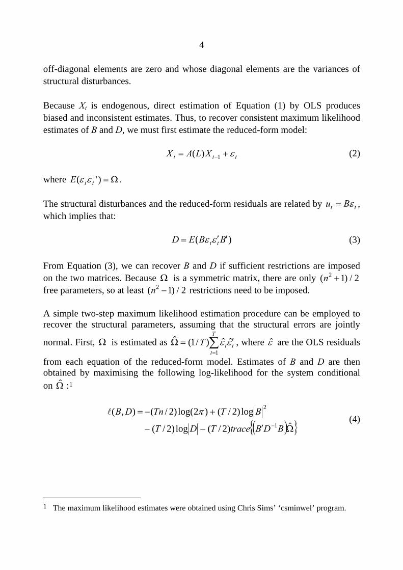
The main aim of this paper is to examine the extent to which interest sensitivity varies across different components of expenditure and production in Australia. Interestingly, Figure 1 suggests that among the expenditure components of GDP, dwelling investment and machinery & equipment investment tend to experience the most significant declines in activity following sustained increases in interest rates, while the fall in durable goods consumption is more moderate. This is in contrast to the US where, as mentioned earlier, machinery & equipment investment has been found to be less interest sensitive than residential investment and durable goods consumption.
The rest of the paper proceeds as follows. In Section 2 we outline the structural vector autoregression (SVAR) model of the Australian economy we use to analyse the sectoral effects of monetary policy. Section 3 then examines the effect of monetary policy shocks on the expenditure and production components of GDP. Section 4 analyses the effect of two other shocks to the system – a consumption shock and a foreign monetary policy shock – and assesses which shocks are most important in explaining the paths of the endogenous variables. In Section 5 we check the robustness of our results to different sample periods, potential-omitted variables and alternative identification assumptions. Section 6 offers some conclusions.
3
Figure 1: Sectoral Activity around Monetary Tightening Episodes
-20
-15
-10
-5
0
5
10
-20
-15
-10
-5
0
5
10
Equipment investment% %
Durable goodsconsumption
Dwelling investment
8620-4-8 4-2-6Quarters after a change in the cash rate
2 Methodology
We use an SVAR to estimate the effect of monetary policy on the different sectors of the economy. SVARs are a straightforward way of capturing important macroeconomic relationships without using a large number of variables or imposing restrictive assumptions on the model. Also, they are commonly used in the literature, allowing us to compare our results with those of other studies.
We assume that the economy can be represented by the following structural form:
ttt uXLCBX += −1)( (1)
where ,0,0)(,)'( ≠∀=′= + suuEDuuE stttt B is a non-singular matrix that is normalised to have 1s on the diagonal, Xt is an 1×n vector of macroeconomic variables, C(L) is a polynomial in the lag operator L, and ut is an vector of structural disturbances. The matrix B summarises the contemporaneous relationship between the endogenous variables, while C(L) summarises how the variables are affected by their own lags as well as the lags of the other variables in the system. The ut are serially uncorrelated and D is a diagonal matrix whose
1×n
4
off-diagonal elements are zero and whose diagonal elements are the variances of structural disturbances.
Because Xt is endogenous, direct estimation of Equation (1) by OLS produces biased and inconsistent estimates. Thus, to recover consistent maximum likelihood estimates of B and D, we must first estimate the reduced-form model:
ttt XLAX ε+= −1)( (2)
where Ω=)'( ttE εε .
The structural disturbances and the reduced-form residuals are related by tt Bu ε= , which implies that:
)( BBED tt ′′= εε (3)
From Equation (3), we can recover B and D if sufficient restrictions are imposed on the two matrices. Because is a symmetric matrix, there are only free parameters, so at least restrictions need to be imposed.
Ω 2/)1( 2 +n2/)1( 2 −n
A simple two-step maximum likelihood estimation procedure can be employed to recover the structural parameters, assuming that the structural errors are jointly
normal. First, Ω is estimated as , where ∑=
′=ΩT
tttT
1ˆˆ)/1(ˆ εε ε̂ are the OLS residuals
from each equation of the reduced-form model. Estimates of B and D are then obtained by maximising the following log-likelihood for the system conditional on :Ω̂ 1
({ Ω′−−
+−=− ˆ)2/(log)2/(
log)2/()2log()2/(),(1
2
BDBtraceTDT
BTTnDB πl
) }
(4)
1 The maximum likelihood estimates were obtained using Chris Sims’ ‘csminwel’ program.
5
A typical way of recovering the structural parameters in an SVAR is to restrict some of B’s off-diagonal elements to be zero. A popular method is to orthogonalise the reduced-form disturbances by Cholesky decomposition, implying a recursive temporal ordering of the variables. An alternative, followed here, is to adopt a set of restrictions informed by economic theory (Bernanke 1986; Sims 1986). Neither approach is without its critics.2 Cooley and Leroy (1995) point out that recursive models have become less popular over time because of the difficulty in finding a theoretically valid causal structure, while others have argued that the results from non-recursive models can be highly sensitive to small changes in the identifying restrictions (Faust 1998). We deal with this issue by employing a range of plausible identifying restrictions to gauge how robust our results are to such changes.
3 A Sectoral Model of the Australian Economy
The first model that we use to analyse the sectoral effects of monetary policy includes all of the following expenditure components of Australian GDP: dwelling investment, machinery & equipment investment, household consumption, exports, imports and a residual term that includes inventories, public demand and the remaining components of business investment.3 In what follows, these variables are stacked so as to form a (6x1) vector Y. Although other specifications were examined, this choice of variables best satisfies the trade-off between including the largest and most cyclical components of GDP, while ensuring that the size of the SVAR remains manageable.
2 An alternative literature identifies SVARs via restrictions on the long-run relationships
between variables (Blanchard and Quah 1989) or restrictions on both contemporaneous and long-run relationships (Galí 1992).
3 We include aggregate consumption in our baseline specification rather than splitting consumption into its durable and non-durable components because we need to limit the size of the SVAR. In an alternative specification (available on request) we found that durable goods consumption was more interest sensitive than non-durable goods, but less interest sensitive than dwelling investment and machinery & equipment investment.
6
We include US GDP (usgdp) to capture the important influence that global economic developments can have on economic conditions in Australia. This approach is consistent with previous Australian VAR studies (Dungey and Pagan 2000; Suzuki 2004; Berkelmans 2005).4
Previous VAR studies have found that the inclusion of commodity prices (pcom) helps to resolve the ‘price puzzle’, in which unexpected increases in interest rates are followed initially by increases in the price level (Sims 1992). Commodity prices have added relevance for the Australian economy because commodities make up a large share of Australia’s total exports.
We include the rate of underlying consumer price inflation (π) rather than the level of the consumer price index because inflation has been the explicit target of monetary policy for more than half of our sample and the underlying series is less noisy (Berkelmans 2005). In addition, the model contains no nominal activity variables, and the rate of change of prices is the logical variable to interact with the real variables and the nominal interest rate.
The inclusion of the overnight cash rate (cash) and a measure of the real exchange rate (rtwi) is standard (Brischetto and Voss 1999; Dungey and Pagan 2000; Berkelmans 2005). The overnight cash rate has been the chief instrument of monetary policy since the float of the dollar in December 1983, which spans our entire sample. The real trade-weighted exchange rate is an important macroeconomic variable in a number of respects, including through its influence on Australia’s trade flows.5
3.1 Identification
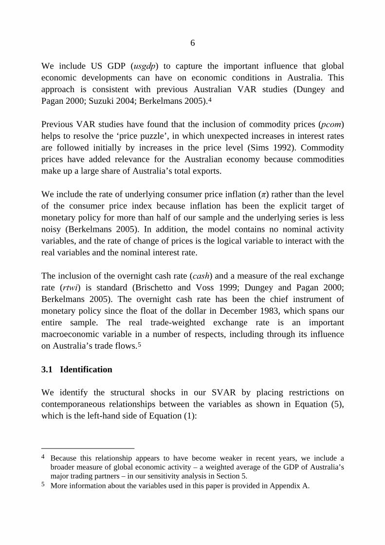
We identify the structural shocks in our SVAR by placing restrictions on contemporaneous relationships between the variables as shown in Equation (5), which is the left-hand side of Equation (1):
4 Because this relationship appears to have become weaker in recent years, we include a
broader measure of global economic activity – a weighted average of the GDP of Australia’s major trading partners – in our sensitivity analysis in Section 5.
5 More information about the variables used in this paper is provided in Appendix A.
7
(5)
⎥⎥⎥⎥⎥⎥⎥
⎦
⎤
⎢⎢⎢⎢⎢⎢⎢
⎣
⎡
⎥⎥⎥⎥⎥⎥⎥⎥
⎦
⎤
⎢⎢⎢⎢⎢⎢⎢⎢
⎣
⎡
≡
−
−
t
t
t
t
t
t
rtwicash
pcomusgdp
bbbbbbb
bb
b
BXπ
tYi2Yi1 YIbb
11000
001000000001000001
10,119,1183,112,111,11
11,102,10
83,992
21
Each non-zero bij coefficient in Equation (5) indicates that variable j affects variable i contemporaneously. The coefficients on the diagonal are normalised to 1, while the other entries in the matrix are constrained to be zero. (Recall that Yt is a (6x1) vector, hence the need for the (6x6) identity matrix I in the matrix B.) The system is over-identified – that is, there are more restrictions than are required to just identify the model.6
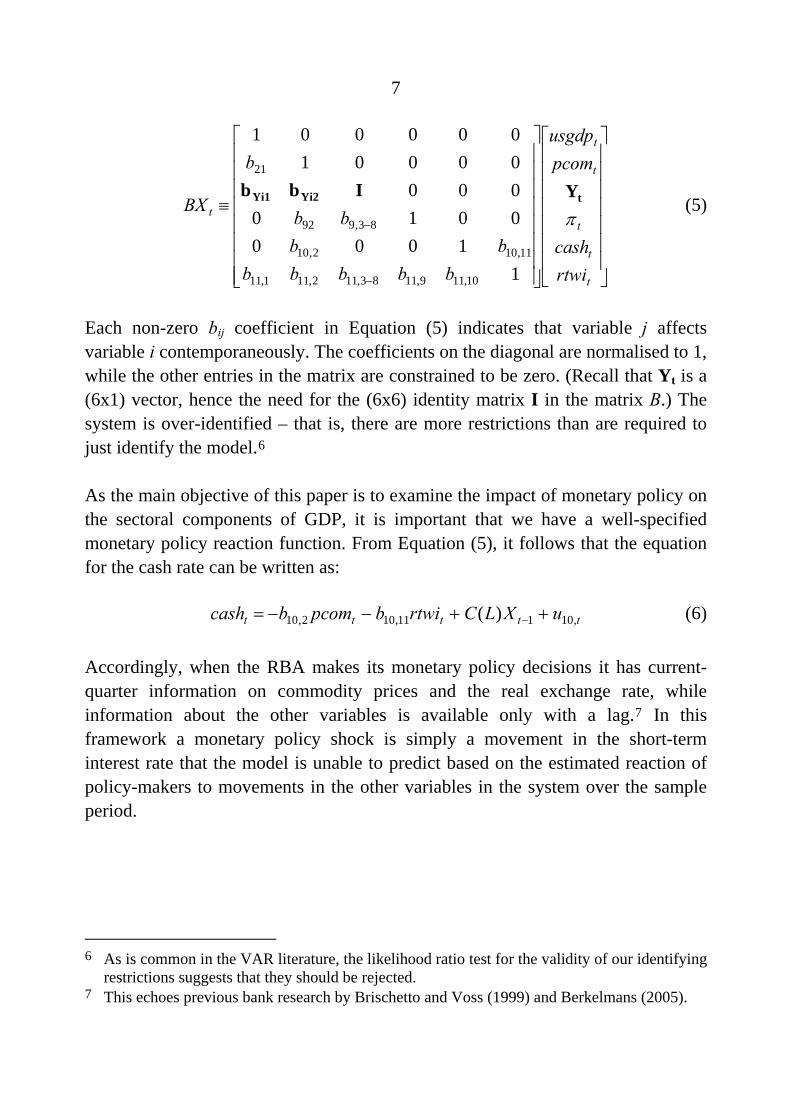
As the main objective of this paper is to examine the impact of monetary policy on the sectoral components of GDP, it is important that we have a well-specified monetary policy reaction function. From Equation (5), it follows that the equation for the cash rate can be written as:
ttttt uXLCrtwibpcombcash ,10111,102,10 )( ++−−= − (6)
Accordingly, when the RBA makes its monetary policy decisions it has current-quarter information on commodity prices and the real exchange rate, while information about the other variables is available only with a lag.7 In this framework a monetary policy shock is simply a movement in the short-term interest rate that the model is unable to predict based on the estimated reaction of policy-makers to movements in the other variables in the system over the sample period.
6 As is common in the VAR literature, the likelihood ratio test for the validity of our identifying
restrictions suggests that they should be rejected. 7 This echoes previous bank research by Brischetto and Voss (1999) and Berkelmans (2005).
8
The explanations for the other restrictions are as follows. The domestic variables are assumed not to affect the foreign variables, reflecting the assumption that Australia is a small open economy (this holds for all lags of the domestic variables as well). US GDP is ordered before commodity prices, which is typical in international VAR studies (Christiano, Eichenbaum and Evans 1996; Cushman and Zha 1997), but is a point of difference from Brischetto and Voss (1999) and Berkelmans (2005). This restriction follows from the observation that, over our sample, large movements in commodity prices have tended to result from fluctuations in the global demand for commodities, rather than the supply-driven price movements that characterised the 1970s.
We allow foreign shocks to affect domestic variables contemporaneously, with two exceptions. The first prevents monetary policy from reacting immediately to shocks to US GDP, reflecting informational lags. The second prevents shocks to US GDP from flowing through to domestic inflation immediately (see Berkelmans 2005).
Following Raddatz and Rigobon (2003), we assume that shocks to individual components of GDP take at least one quarter to affect the other components of GDP (as reflected in the (6x6) identity matrix, I). Placing some restrictions on the contemporaneous relationships between the GDP components is necessary to identify the SVAR. In our sensitivity analysis we consider an alternative recursive identification of the GDP components. However, a recursive identification is not our preferred method because of the difficulty in coming up with a convincing theoretical justification for any particular temporal ordering of the GDP components.
We allow inflation to respond contemporaneously to domestic output. This assumption is common in both domestic (Brischetto and Voss 1999; Dungey and Pagan 2000; Berkelmans 2005) and international (Bernanke and Blinder 1992) studies. Other domestic variables affect inflation only with a lag of one quarter (see Section 5 for further discussion of this point). Finally, the real exchange rate is assumed to respond contemporaneously to all other variables, as is common in VAR studies.
9
3.2 Estimation
The model is estimated using quarterly data from December 1983 to September 2007, yielding 96 observations. By restricting the sample to the post-float period, our results should be less vulnerable to parameter instability. However, even over this relatively short period there have been significant changes in the conduct of monetary policy (such as the move to inflation targeting in 1993) and other structural changes to the economy. We deal with this in our sensitivity analysis by comparing the results from our baseline model to those from models estimated over two shorter sub-samples. In all cases the impulse responses should be interpreted as representing sample averages rather than how the economy would respond to shocks today.
In our baseline specification, all variables enter the model in log-levels, with the exception of the inflation rate and the cash rate, which enter in percentage point terms. Although unit root tests suggest that many of the variables in the SVAR are likely to be non-stationary, estimation in levels is still consistent and avoids losing information about possible long-run relationships between the variables in our model (Sims 1980; Sims, Stock and Watson 1990).8 It is also the approach most commonly taken in the SVAR literature.9
Correct specification of the model also requires the inclusion of the appropriate number of lags. If too few lags are included, the residuals may not be white noise and hence standard inference is inappropriate. On the other hand, including too many lags risks over-parameterising the model (Hamilton 1994). Our specification tests (Akaike Information Criterion (AIC) and the Schwartz Bayesian Information Criterion (BIC)) suggest that either three, four or five lags are optimal. While we use three to reduce the number of parameters to be estimated, the results are largely insensitive to this choice.
8 Results of the unit root tests are available from the authors. 9 As a robustness check, we estimated our model with all variables other than the cash rate
expressed as quarterly percentage changes. This transformation did not alter the relative responsiveness of the components of domestic GDP to a monetary policy shock. However, the response of inflation to a monetary policy shock is strongly positive for several quarters, reinforcing our preference for our baseline model. The inclusion of a linear time trend and dummy variables for the period around the introduction of the Goods and Services Tax in 2000 also had little effect on our core results.
10
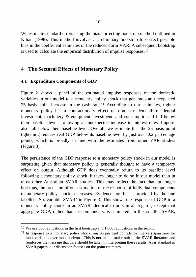
We estimate standard errors using the bias-correcting bootstrap method outlined in Kilian (1998). This method involves a preliminary bootstrap to correct possible bias in the coefficient estimates of the reduced-form VAR. A subsequent bootstrap is used to calculate the empirical distribution of impulse responses.10
4 The Sectoral Effects of Monetary Policy
4.1 Expenditure Components of GDP
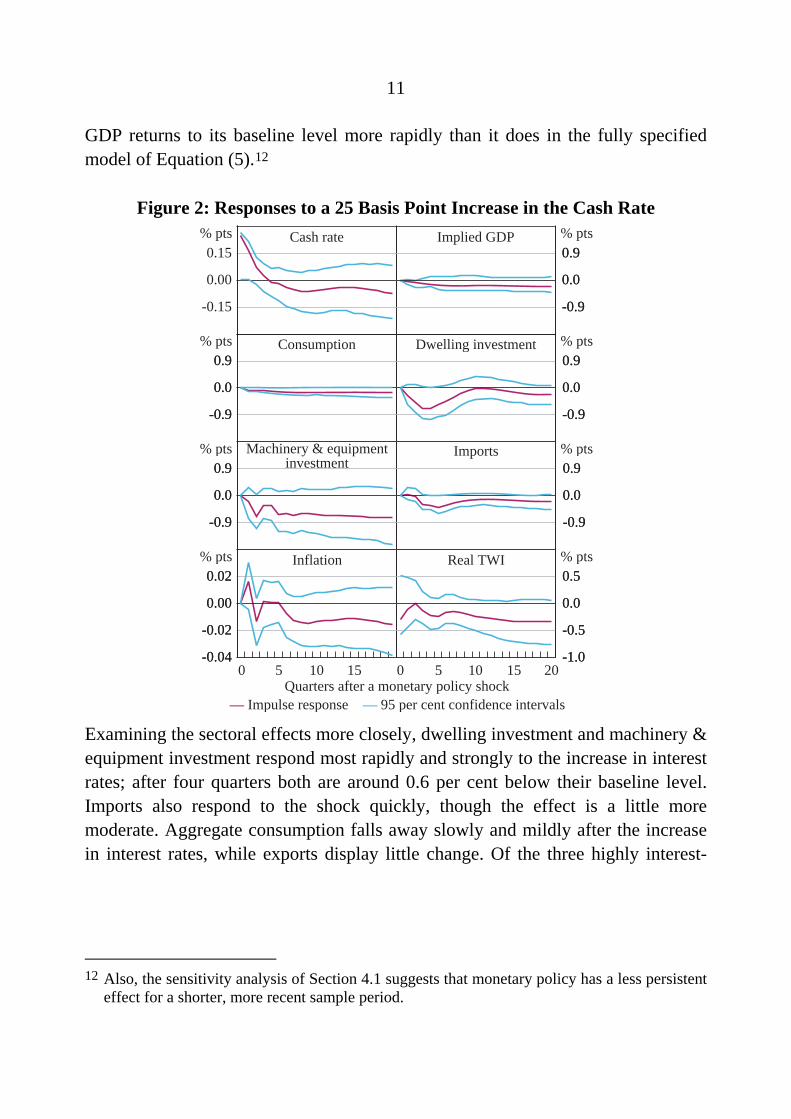
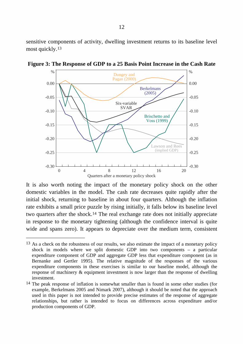
Figure 2 shows a panel of the estimated impulse responses of the domestic variables in our model to a monetary policy shock that generates an unexpected 25 basis point increase in the cash rate.11 According to our estimates, tighter monetary policy has a contractionary effect on domestic demand: residential investment, machinery & equipment investment, and consumption all fall below their baseline levels following an unexpected increase in interest rates. Imports also fall below their baseline level. Overall, we estimate that the 25 basis point tightening reduces real GDP below its baseline level by just over 0.2 percentage points, which is broadly in line with the estimates from other VAR studies (Figure 3).
The persistence of the GDP response to a monetary policy shock in our model is surprising given that monetary policy is generally thought to have a temporary effect on output. Although GDP does eventually return to its baseline level following a monetary policy shock, it takes longer to do so in our model than in most other Australian SVAR studies. This may reflect the fact that, at longer horizons, the precision of our estimation of the response of individual components to monetary policy shocks decreases. Evidence for this is provided by the line labelled ‘Six-variable SVAR’ in Figure 3. This shows the response of GDP to a monetary policy shock in an SVAR identical to ours in all regards, except that aggregate GDP, rather than its components, is estimated. In this smaller SVAR,
10 We use 500 replications in the first bootstrap and 1 000 replications in the second. 11 In response to a monetary policy shock, our 95 per cent confidence intervals span zero for
most variables over most horizons. This is not an unusual result in the SVAR literature and reinforces the message that care should be taken in interpreting these results. As is standard in SVAR papers, our discussion focuses on the point estimates.
11
GDP returns to its baseline level more rapidly than it does in the fully specified model of Equation (5).12
Figure 2: Responses to a 25 Basis Point Increase in the Cash Rate
-0.15
0.00
0.15
Quarters after a monetary policy shock
-0.04
-0.02
0.00
0.02
-0.04
-0.02
0.00
0.02
-0.9
0.0
0.9
-0.9
0.0
0.9
-1.0
-0.5
0.0
0.5
-1.0
-0.5
0.0
0.5
-0.9
0.0
0.9
-0.9
0.0
0.9
-0.9
0.0
0.9
-0.9
0.0
0.9
-0.9
0.0
0.9
-0.9
0.0
0.9
-0.9
0.0
0.9
-0.9
0.0
0.9
Cash rate Implied GDP
Consumption Dwelling investment
Machinery & equipmentinvestment
Imports
Inflation Real TWI
% pts
0 2015105151050
— Impulse response — 95 per cent confidence intervals
% pts
% pts
% pts
% pts
% pts
% pts
% pts
Examining the sectoral effects more closely, dwelling investment and machinery & equipment investment respond most rapidly and strongly to the increase in interest rates; after four quarters both are around 0.6 per cent below their baseline level. Imports also respond to the shock quickly, though the effect is a little more moderate. Aggregate consumption falls away slowly and mildly after the increase in interest rates, while exports display little change. Of the three highly interest-
12 Also, the sensitivity analysis of Section 4.1 suggests that monetary policy has a less persistent
effect for a shorter, more recent sample period.
12
sensitive components of activity, dwelling investment returns to its baseline level most quickly.13
Figure 3: The Response of GDP to a 25 Basis Point Increase in the Cash Rate
-0.30
-0.25
-0.20
-0.15
-0.10
-0.05
0.00
-0.30
-0.25
-0.20
-0.15
-0.10
-0.05
0.00
Brischetto andVoss (1999)
% %
Lawson and Rees
Berkelmans(2005)
2084Quarters after a monetary policy shock
120
Dungey andPagan (2000)
16
Six-variableSVAR
(implied GDP)
It is also worth noting the impact of the monetary policy shock on the other domestic variables in the model. The cash rate decreases quite rapidly after the initial shock, returning to baseline in about four quarters. Although the inflation rate exhibits a small price puzzle by rising initially, it falls below its baseline level two quarters after the shock.14 The real exchange rate does not initially appreciate in response to the monetary tightening (although the confidence interval is quite wide and spans zero). It appears to depreciate over the medium term, consistent 13 As a check on the robustness of our results, we also estimate the impact of a monetary policy
shock in models where we split domestic GDP into two components – a particular expenditure component of GDP and aggregate GDP less that expenditure component (as in Bernanke and Gertler 1995). The relative magnitude of the responses of the various expenditure components in these exercises is similar to our baseline model, although the response of machinery & equipment investment is now larger than the response of dwelling investment.
14 The peak response of inflation is somewhat smaller than is found in some other studies (for example, Berkelmans 2005 and Nimark 2007), although it should be noted that the approach used in this paper is not intended to provide precise estimates of the response of aggregate relationships, but rather is intended to focus on differences across expenditure and/or production components of GDP.
13
with uncovered interest parity. As the responses of these non-GDP variables to a monetary policy shock are similar across the models that we study, we will not discuss them in detail in the remainder of the paper.
Although the sectoral results are broadly in line with our expectations, the fact that machinery & equipment investment is just as responsive to monetary policy as dwelling investment is interesting given that empirical studies in the US have found residential investment to be considerably more interest sensitive (Raddatz and Rigobon 2003; Bernanke and Gertler 1995). One possible explanation is that Australian firms may be more dependent on bank finance than their American counterparts (and so monetary policy may have a relatively strong effect on Australian business investment via the cash-flow channel). This certainly accords with the large contraction in machinery & equipment investment during the early 1990s recession in Australia when credit growth to businesses may have been constrained by supply-side considerations (Tallman and Bharucha 2000). The moderate effect of monetary policy on consumption makes sense when we remember that durable goods make up only 20 per cent of aggregate consumption. Note also that because consumption is a much larger share of aggregate activity than residential investment and machinery & equipment investment, it makes the largest contribution to the fall in GDP.
4.2 Production Components of GDP
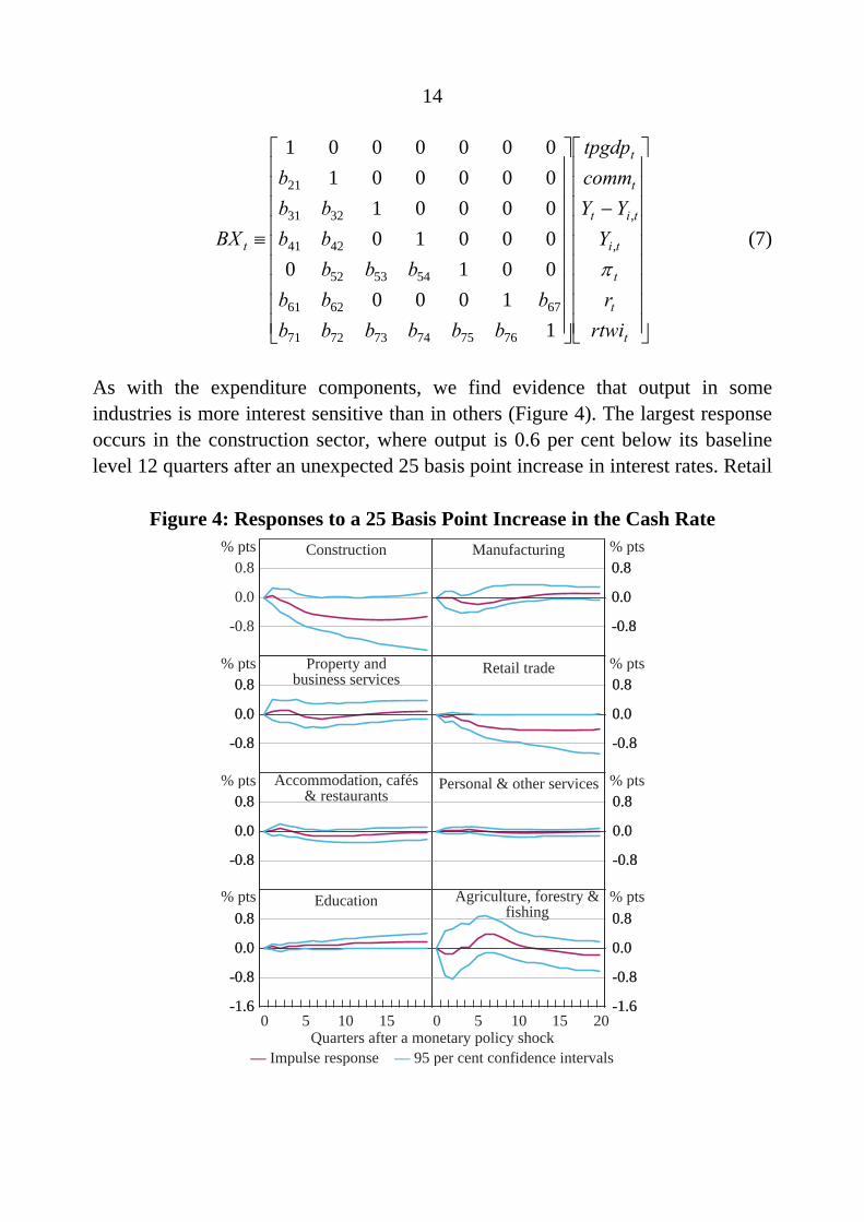
We can also examine the effect of monetary policy across different industries. Because there are too many industries to include in a single SVAR, we estimate a separate model for each industry – an approach similar to that used by Bernanke and Gertler (1995). Equation (7) shows the identification scheme for each industry regression. This is similar to the expenditure components model, except there are only two domestic activity variables in each model – output in the industry of interest ( ), and output in all other industries ( ). A potential problem with this approach is that the monetary surprises we estimate in each industry model may not be identical. However, our results suggest that structural errors in the interest rate equation are similar in each industry regression.
tiY , tit YY ,−
14
(7)
⎥⎥⎥⎥⎥⎥⎥⎥⎥
⎦
⎤
⎢⎢⎢⎢⎢⎢⎢⎢⎢
⎣
⎡
−
⎥⎥⎥⎥⎥⎥⎥⎥⎥
⎦
⎤
⎢⎢⎢⎢⎢⎢⎢⎢⎢
⎣
⎡
≡
t
t
t
ti
tit
t
t
t
rtwir
YYY
commtpgdp
bbbbbbbbb
bbbbbbb
b
BXπ
,
,
767574737271
676261
545352
4241
3231
21
11000
001000010000010000010000001
As with the expenditure components, we find evidence that output in some industries is more interest sensitive than in others (Figure 4). The largest response occurs in the construction sector, where output is 0.6 per cent below its baseline level 12 quarters after an unexpected 25 basis point increase in interest rates. Retail
Figure 4: Responses to a 25 Basis Point Increase in the Cash Rate
-0.8
0.0
0.8
Quarters after a monetary policy shock
-1.6
-0.8
0.0
0.8
-1.6
-0.8
0.0
0.8
-0.8
0.0
0.8
-0.8
0.0
0.8
-1.6
-0.8
0.0
0.8
-1.6
-0.8
0.0
0.8
-0.8
0.0
0.8
-0.8
0.0
0.8
-0.8
0.0
0.8
-0.8
0.0
0.8
-0.8
0.0
0.8
-0.8
0.0
0.8
-0.8
0.0
0.8
-0.8
0.0
0.8
Construction Manufacturing
Property andbusiness services
Retail trade
Accommodation, cafés& restaurants
Personal & other services
Agriculture, forestry &fishing
Education
% pts
015 20151051050
— Impulse response — 95 per cent confidence intervals
% pts
% pts
% pts
% pts
% pts
% pts
% pts
15
trade and manufacturing also decline, falling 0.4 per cent and 0.2 per cent, respectively, below their baseline levels 18 months after a contractionary monetary policy shock. These responses are broadly consistent with the results from the expenditure components model. In particular, the large decline in residential investment is consistent with the fall in production in the construction sector, while the relatively large response of retail trade probably reflects that sector’s larger exposure to durable goods consumption than is the case for aggregate consumption. Among the least interest-sensitive industries are education, government administration, mining and agriculture, where supply-side factors are likely to be more important.
4.3 The Effect of a Shock to Domestic Consumption
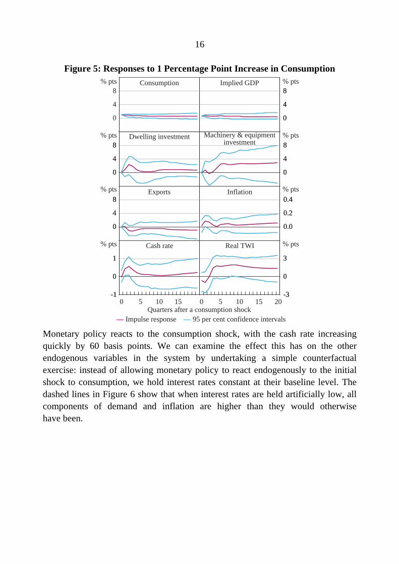
These models of the Australian economy can also help us to understand the response of the economy to shocks to key variables besides interest rates. Using our expenditure SVAR, we first examine the impact of a shock to household consumption which, given its large share of aggregate GDP, is a potentially important source of shocks to the domestic economy. Figure 5 shows that, following an unexpected 1 percentage point increase in consumption, there is a noticeable expansion in residential investment and machinery & equipment investment while exports fall. This increase in domestic demand causes an increase in the rate of inflation and an appreciation of the real exchange rate.15
15 Although the shock to consumption should not be given an explicit structural interpretation
(because other variables that influence consumption, such as employment growth and household wealth, are not included in the model), the fact that both output and inflation increase following the shock is consistent with a positive shock to demand.
16
Figure 5: Responses to 1 Percentage Point Increase in Consumption
0
4
8
-1
0
1
-1
0
1
0
4
8
0
4
8
-3
0
3
-3
0
3
0
4
8
0
4
8
0.0
0.2
0.4
0.0
0.2
0.4
0
4
8
0
4
8
0
4
8
0
4
8
Consumption Implied GDP
Dwelling investment Machinery & equipmentinvestment
Exports Inflation
Cash rate Real TWI
% pts
0 201550Quarters after a consumption shock
10155 10
— Impulse response — 95 per cent confidence intervals
% pts
% pts
% pts
% pts
% pts
% pts
% pts
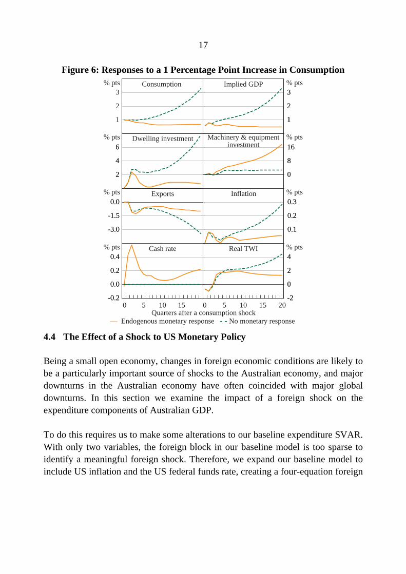
Monetary policy reacts to the consumption shock, with the cash rate increasing quickly by 60 basis points. We can examine the effect this has on the other endogenous variables in the system by undertaking a simple counterfactual exercise: instead of allowing monetary policy to react endogenously to the initial shock to consumption, we hold interest rates constant at their baseline level. The dashed lines in Figure 6 show that when interest rates are held artificially low, all components of demand and inflation are higher than they would otherwise have been.
17
Figure 6: Responses to a 1 Percentage Point Increase in Consumption
1
2
3
Quarters after a consumption shock
-0.2
0.0
0.2
0.4
-0.2
0.0
0.2
0.4
1
2
3
1
2
3
-2
0
2
4
-2
0
2
4
-3.0
-1.5
0.0
-3.0
-1.5
0.0
0.1
0.2
0.3
0.1
0.2
0.3
2
4
6
2
4
6
0
8
16
0
8
16
Cash rate
Machinery & equipmentinvestment
Dwelling investment
Consumption Implied GDP
Exports Inflation
Real TWI
% pts
— Endogenous monetary response - - No monetary response
0 201550 10155 10
% pts
% pts
% pts
% pts
% pts
% pts
% pts
4.4 The Effect of a Shock to US Monetary Policy
Being a small open economy, changes in foreign economic conditions are likely to be a particularly important source of shocks to the Australian economy, and major downturns in the Australian economy have often coincided with major global downturns. In this section we examine the impact of a foreign shock on the expenditure components of Australian GDP.
To do this requires us to make some alterations to our baseline expenditure SVAR. With only two variables, the foreign block in our baseline model is too sparse to identify a meaningful foreign shock. Therefore, we expand our baseline model to include US inflation and the US federal funds rate, creating a four-equation foreign
18
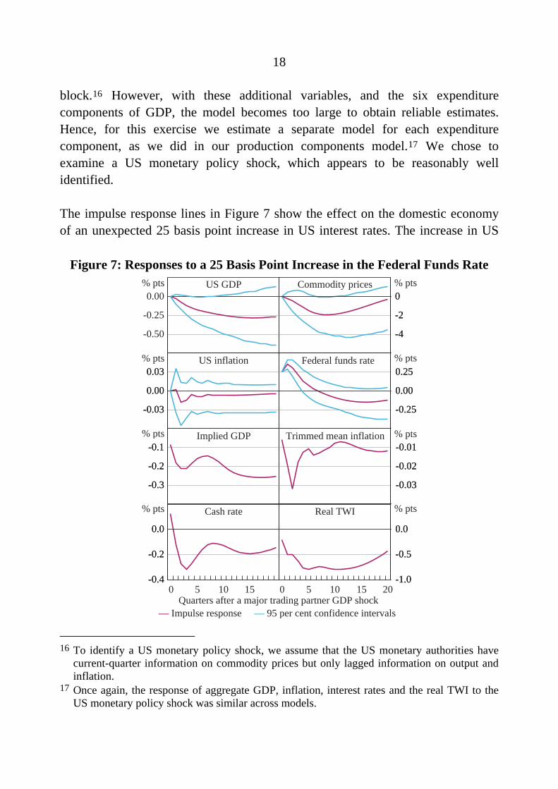
block.16 However, with these additional variables, and the six expenditure components of GDP, the model becomes too large to obtain reliable estimates. Hence, for this exercise we estimate a separate model for each expenditure component, as we did in our production components model.17 We chose to examine a US monetary policy shock, which appears to be reasonably well identified.
The impulse response lines in Figure 7 show the effect on the domestic economy of an unexpected 25 basis point increase in US interest rates. The increase in US
Figure 7: Responses to a 25 Basis Point Increase in the Federal Funds Rate
-0.50
-0.25
0.00
Quarters after a major trading partner GDP shock
-0.4
-0.2
0.0
-0.4
-0.2
0.0
-4
-2
0
-4
-2
0
-1.0
-0.5
0.0
-1.0
-0.5
0.0
-0.3
-0.2
-0.1
-0.3
-0.2
-0.1
-0.03
-0.02
-0.01
-0.03
-0.02
-0.01
-0.03
0.00
0.03
-0.03
0.00
0.03
-0.25
0.00
0.25
-0.25
0.00
0.25
Cash rate
Commodity pricesUS GDP
US inflation Federal funds rate
Implied GDP Trimmed mean inflation
Real TWI
% pts
0 201550
— Impulse response — 95 per cent confidence intervals
10155 10
% pts
% pts
% pts
% pts
% pts
% pts
% pts
16 To identify a US monetary policy shock, we assume that the US monetary authorities have
current-quarter information on commodity prices but only lagged information on output and inflation.
17 Once again, the response of aggregate GDP, inflation, interest rates and the real TWI to the US monetary policy shock was similar across models.
19
interest rates has the expected impact on the foreign variables in the model – commodity prices, US output and US inflation all fall below their baseline levels. The decrease in foreign activity has a pronounced effect on the domestic economy – dwelling investment, machinery & equipment investment and consumption all decline. Inflation also falls, which leads interest rates to fall by 30 basis points four quarters after the shock. The real exchange rate depreciates after the shock, which cushions the impact of the shock on the traded-goods sector and contributes to an increase in exports, presumably to countries other than the US.
Replicating our simple counterfactual exercise, when domestic interest rates are held artificially high, all components of demand and inflation are lower than they would otherwise have been (results not shown). This suggests that over our sample period, Australian monetary policy has helped to dampen the impact of foreign shocks.
5 Which Shocks Are Most Important?
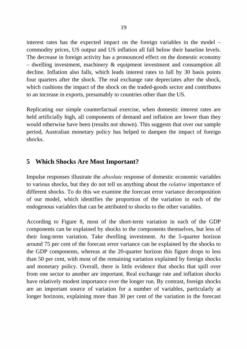
Impulse responses illustrate the absolute response of domestic economic variables to various shocks, but they do not tell us anything about the relative importance of different shocks. To do this we examine the forecast error variance decomposition of our model, which identifies the proportion of the variation in each of the endogenous variables that can be attributed to shocks to the other variables.
According to Figure 8, most of the short-term variation in each of the GDP components can be explained by shocks to the components themselves, but less of their long-term variation. Take dwelling investment. At the 5-quarter horizon around 75 per cent of the forecast error variance can be explained by the shocks to the GDP components, whereas at the 20-quarter horizon this figure drops to less than 50 per cent, with most of the remaining variation explained by foreign shocks and monetary policy. Overall, there is little evidence that shocks that spill over from one sector to another are important. Real exchange rate and inflation shocks have relatively modest importance over the longer run. By contrast, foreign shocks are an important source of variation for a number of variables, particularly at longer horizons, explaining more than 30 per cent of the variation in the forecast
20
errors for dwelling investment, machinery & equipment investment, imports, exports, inflation, the cash rate and the real exchange rate after 20 quarters.
Figure 8: Forecast Error Variance Decomposition
25
50
75
25
50
75
25
50
75
Forecast (quarters)
0
25
50
75
0
25
50
75
25
50
75
25
50
75
0
25
50
75
0
25
50
75
25
50
75
25
50
75
25
50
75
25
50
75
25
50
75
25
50
75
Cash rate
Trimmed mean inflation
Consumption Dwelling investment
Machinery & equipmentinvestment
Exports
Imports
Real TWI
% %
%
%
%
%
%
%
— Foreign — GDP components— Monetary policy
1 7 13 19 1 7 13 19
— Other
6 Sensitivity Analysis
6.1 Sample Period
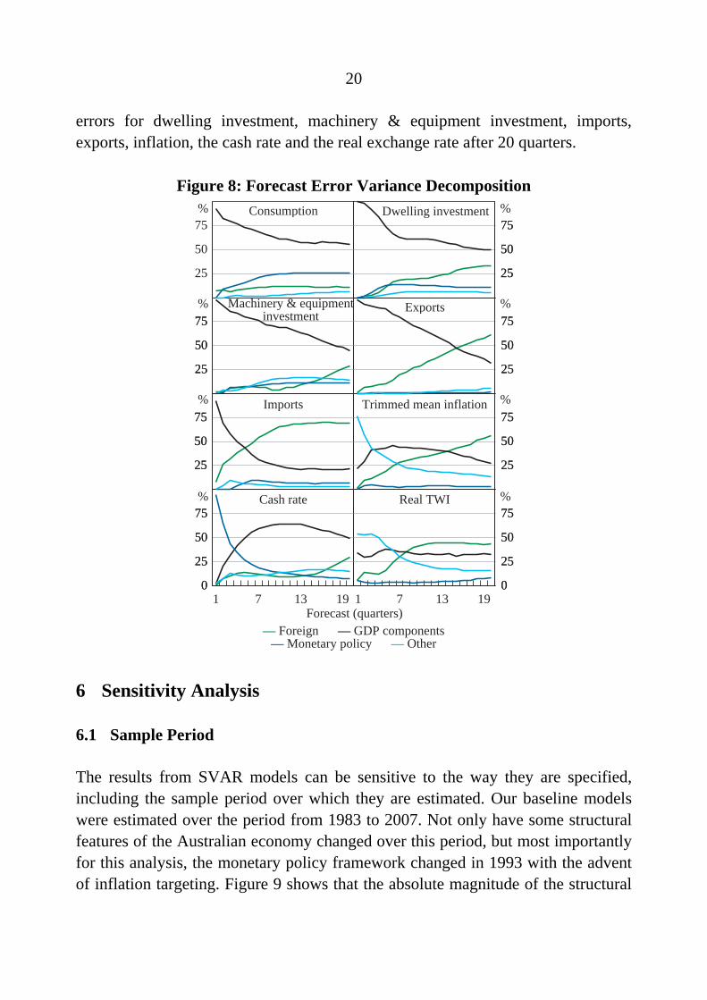
The results from SVAR models can be sensitive to the way they are specified, including the sample period over which they are estimated. Our baseline models were estimated over the period from 1983 to 2007. Not only have some structural features of the Australian economy changed over this period, but most importantly for this analysis, the monetary policy framework changed in 1993 with the advent of inflation targeting. Figure 9 shows that the absolute magnitude of the structural
21
shocks in the cash rate equation has declined significantly in the second half of our sample period, suggesting that monetary policy has become more predictable.18
Figure 9: Estimated Structural Shocks Absolute values
0.4
0.8
1.2
0.5
1.0
1.5
0
6
12
18
0.5
1.0
1.5
0
4
8
12
3
6
9
Dwelling investment
US GDP Cash rate
Consumption Machinery & equipmentinvestment
Commodity prices
% %
%
%
%
%
20072007 199719971987 To examine whether the relative interest sensitivity of different sectors is influenced by our sample period, we re-estimate our expenditure components model over two periods – March 1981 to September 1997, and March 1991 to September 2007. Each sample contains 67 observations and we have chosen them to minimise the number of overlapping observations while leaving us with enough degrees of freedom to estimate the model.
18 For ease of interpretation, we have converted the structural errors to absolute values.
22
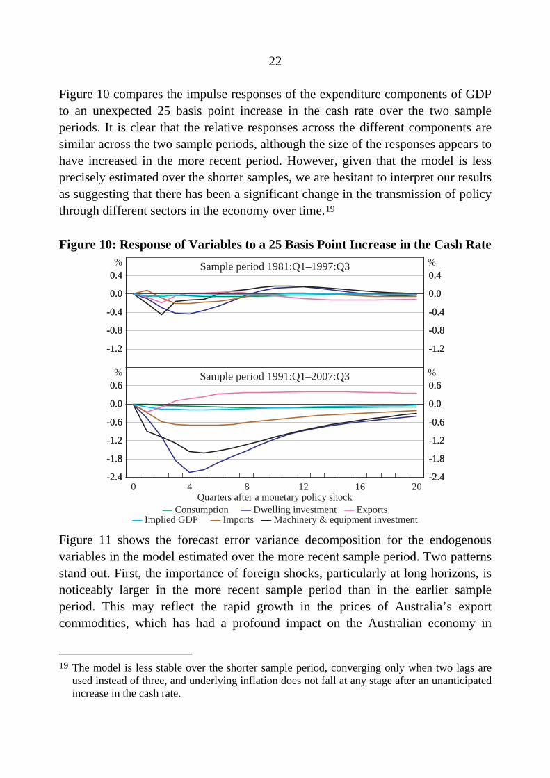
Figure 10 compares the impulse responses of the expenditure components of GDP to an unexpected 25 basis point increase in the cash rate over the two sample periods. It is clear that the relative responses across the different components are similar across the two sample periods, although the size of the responses appears to have increased in the more recent period. However, given that the model is less precisely estimated over the shorter samples, we are hesitant to interpret our results as suggesting that there has been a significant change in the transmission of policy through different sectors in the economy over time.19
Figure 10: Response of Variables to a 25 Basis Point Increase in the Cash Rate
-2.4
-1.8
-1.2
-0.6
0.0
0.6
-2.4
-1.8
-1.2
-0.6
0.0
0.6
-2.4
-1.8
-1.2
-0.6
0.0
0.6
-2.4
-1.8
-1.2
-0.6
0.0
0.6
-1.2
-0.8
-0.4
0.0
0.4
-1.2
-0.8
-0.4
0.0
0.4
-1.2
-0.8
-0.4
0.0
0.4
-1.2
-0.8
-0.4
0.0
0.4
20
Sample period 1991:Q1–2007:Q3
Sample period 1981:Q1–1997:Q3
1612840
% %
%%
Quarters after a monetary policy shock— Consumption — Dwelling investment — Exports
— Implied GDP — Imports — Machinery & equipment investment
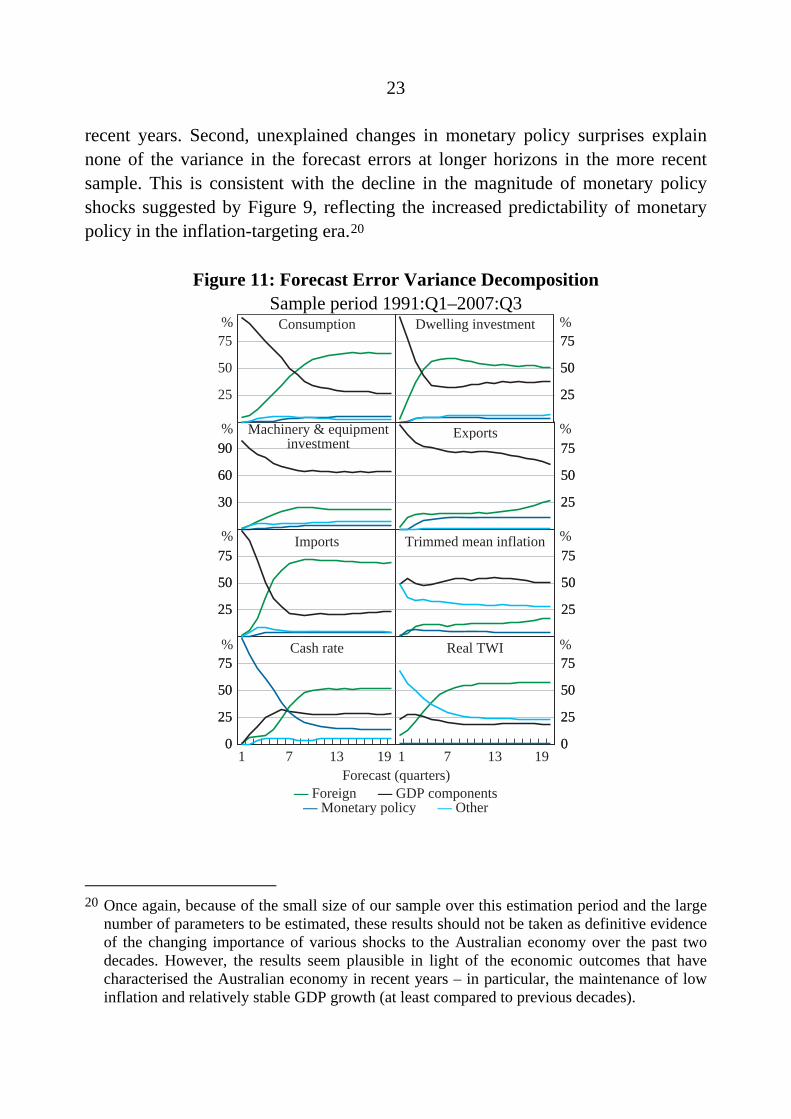
Figure 11 shows the forecast error variance decomposition for the endogenous variables in the model estimated over the more recent sample period. Two patterns stand out. First, the importance of foreign shocks, particularly at long horizons, is noticeably larger in the more recent sample period than in the earlier sample period. This may reflect the rapid growth in the prices of Australia’s export commodities, which has had a profound impact on the Australian economy in
19 The model is less stable over the shorter sample period, converging only when two lags are
used instead of three, and underlying inflation does not fall at any stage after an unanticipated increase in the cash rate.
23
recent years. Second, unexplained changes in monetary policy surprises explain none of the variance in the forecast errors at longer horizons in the more recent sample. This is consistent with the decline in the magnitude of monetary policy shocks suggested by Figure 9, reflecting the increased predictability of monetary policy in the inflation-targeting era.20
Figure 11: Forecast Error Variance Decomposition Sample period 1991:Q1–2007:Q3
30
60
90
30
60
90
25
50
75
Forecast (quarters)
0
25
50
75
0
25
50
75
25
50
75
25
50
75
0
25
50
75
0
25
50
75
25
50
75
25
50
75
25
50
75
25
50
75
25
50
75
25
50
75
Cash rate
Trimmed mean inflation
Consumption Dwelling investment
Machinery & equipmentinvestment
Exports
Imports
Real TWI
% %
%
%
%
%
%
%
— Foreign — GDP components— Monetary policy
1 7 13 19 1 7 13 19
— Other
20 Once again, because of the small size of our sample over this estimation period and the large
number of parameters to be estimated, these results should not be taken as definitive evidence of the changing importance of various shocks to the Australian economy over the past two decades. However, the results seem plausible in light of the economic outcomes that have characterised the Australian economy in recent years – in particular, the maintenance of low inflation and relatively stable GDP growth (at least compared to previous decades).
24
6.2 Omitted Variables
We also examine whether our results are robust to the choice of variables in our baseline specifications. First, we include major trading partner GDP instead of US GDP as our measure of global economic activity to better capture the effect of the recent rapid growth of countries such as China. The inclusion of major trading partner GDP leaves our key results broadly intact, although there is an increase in the interest sensitivity of dwelling investment relative to our baseline model, which implies a slightly larger decline in aggregate GDP in response to a positive interest rate shock, although it also returns to its baseline level more rapidly.
We also estimate models including variables such as total credit (which may be correlated with the cash rate) and household net wealth (which may be correlated with dwelling investment and consumption).21 The alternative variables have little effect on our core results. The inclusion of the wealth variable increases the interest sensitivity of consumption slightly.
6.3 Identification Schemes
Finally, we experimented with alternative identification schemes such as the recursive scheme proposed by Christiano et al (1996), in which monetary policy responds to GDP and inflation contemporaneously, but these variables respond to monetary policy only with a lag. Again, the relative sensitivity of the sectors is largely unchanged.
7 Conclusion
Using a sectoral SVAR we find evidence that the two most interest-sensitive expenditure components of GDP are residential investment and machinery & equipment investment, while the most interest-sensitive production components of GDP are construction and retail trade. We also present evidence showing that monetary policy has helped to dampen the effect of US monetary policy and domestic consumption shocks.
21 See Berkelmans (2005) for a detailed VAR study of the role of credit in the transmission of
monetary policy.
25
The results are largely robust to the inclusion of additional variables, alternative identification schemes and the sample period over which the model is estimated. There is some weak evidence that the investment components of GDP have become more interest sensitive over time. We also found that large monetary policy shocks have become less prevalent in the inflation-targeting period, consistent with the proposition that monetary policy has become more transparent and predictable. Foreign shocks appear to have become correspondingly more important in explaining the variation in domestic activity.
26
Appendix A: Data Descriptions and Sources
US real gross domestic product: The natural logarithm of seasonally adjusted (sa) quarterly real US GDP (Datastream code: USGDP…D).
Real commodity prices: The Economist index of commodity prices in US dollars (Datastream code: ECALLI$).
Australian real gross domestic product: All production and expenditure components of GDP are expressed in natural logarithms and are sa (ABS Cat No 5206.0).
Australian inflation: Quarterly inflation of the trimmed mean consumer price index excluding taxes and interest (Reserve Bank of Australia (RBA)).
Overnight cash rate: Overnight cash rate, averaged over the quarter. Nominal official cash rate until June 1998, and then the interbank overnight rate (RBA).
Real trade-weighted index: The natural logarithm of the real trade-weighted exchange rate index (RBA).
Australian major trading partner gross domestic product: The natural logarithm of quarterly sa Australian major trading partner real GDP (RBA).
Real break-adjusted credit: The natural logarithm of sa break-adjusted Australian credit (RBA Bulletin Table D.2) deflated by the trimmed mean consumer price index excluding taxes and interest (RBA).
US federal funds rate: The US federal funds target rate, averaged over the quarter (Datastream code: USFDTRG).
US inflation: Quarterly inflation of the chain price index for personal consumption (Datastream code: USCE…E).
Household non-financial assets: The natural logarithm of household non-financial assets (RBA) deflated by the trimmed mean consumer price inflation index (RBA).
27
References
Beechey M, N Bharucha, A Cagliarini, D Gruen and C Thompson (2000), ‘A Small Model of the Australian Macroeconomy’, RBA Research Discussion Paper No 2000-05.
Berkelmans L (2005), ‘Credit and Monetary Policy: An Australian SVAR’, RBA Research Discussion Paper No 2005-06.
Bernanke BS (1986), ‘Alternative Explanations of the Money-Income Correlation’, NBER Working Paper No 1842.
Bernanke BS and AS Blinder (1992), ‘The Federal Funds Rate and the Channels of Monetary Transmission’, American Economic Review, 82(4), pp 901–921.
Bernanke BS and M Gertler (1995), ‘Inside the Black Box: The Credit Channel of Monetary Policy Transmission’, Journal of Economic Perspectives, 9(4), pp 27–48.
Blanchard OJ and D Quah (1989), ‘The Dynamic Effects of Aggregate Demand and Supply Disturbances’, American Economic Review, 79(4), pp 655–673.
Brischetto A and G Voss (1999), ‘A Structural Vector Autoregression Model of Monetary Policy in Australia’, RBA Research Discussion Paper No 1999-11.
Carlino G and R DeFina (1998), ‘The Differential Regional Effects of Monetary Policy’, Review of Economics and Statistics, 80(4), pp 572–587.
Christiano LJ, M Eichenbaum and C Evans (1996), ‘The Effects of Monetary Policy Shocks: Evidence from the Flow of Funds’, Review of Economics and Statistics, 78(1), pp 16–34.
Cooley TF and SF Leroy (1985), ‘Atheoretical Macroeconometrics: A Critique’, Journal of Monetary Economics, 16(3), pp 283–308.
28
Cushman DO and T Zha (1997), ‘Identifying Monetary Policy in a Small Open Economy under Flexible Exchange Rates’, Journal of Monetary Economics, 39(3), pp 433–448.
Dale S and AG Haldane (1995), ‘Interest Rates and the Channels of Monetary Transmission: Some Sectoral Estimates’, European Economic Review, 39(9), pp 1611–1626.
Dedola L and F Lippi (2005), ‘The Monetary Transmission Mechanism: Evidence from the Industries of Five OECD Countries’, European Economic Review, 49(6), pp 1543–1569.
Dungey M and A Pagan (2000), ‘A Structural VAR Model of the Australian Economy’, Economic Record, 76(235), pp 321–342.
Faust J (1998), ‘The Robustness of Identified VAR Conclusions about Money’, Board of Governors of the Federal Reserve System International Finance Discussion Paper No 610.
Galí J (1992), ‘How Well Does the IS-LM Model Fit Post-War US Data?’, Quarterly Journal of Economics, 107(2), pp 709–738.
Hamilton JD (1994), Time Series Analysis, Princeton University Press, Princeton.
Kilian L (1998), ‘Small-Sample Confidence Intervals for Impulse Response Functions’, Review of Economics and Statistics, 80(2), pp 218–230.
Meltzer AH (1995), ‘Monetary, Credit and (Other) Transmission Processes: A Monetarist Perspective’, Journal of Economic Perspectives, 9(4), pp 49–72.
Mishkin FS (1996), ‘The Channels of Monetary Transmission: Lessons for Monetary Policy’, NBER Working Paper No 5464.
Mishkin FS (2007), ‘Housing and the Monetary Transmission Mechanism’, NBER Working Paper No 13518.
29
Nimark K (2007), ‘A Structural Model of Australia as a Small Open Economy’, RBA Research Discussion Paper No 2007-01.
Raddatz C and R Rigobon (2003), ‘Monetary Policy and Sectoral Shocks: Did the Federal Reserve React Properly to the High-Tech Crisis?’, World Bank Policy Research Working Paper Series No 3160.
Sims CA (1980), ‘Macroeconomics and Reality’, Econometrica, 48(1), pp 1–48.
Sims CA (1986), ‘Are Forecasting Models Usable for Policy Analysis?’, Federal Reserve Bank of Minneapolis Quarterly Review, 10(1), pp 2–16.
Sims CA (1992), ‘Interpreting the Macroeconomic Time Series Facts: The Effects of Monetary Policy’, European Economic Review, 36(5), pp 975–1000.
Sims CA, JH Stock and MW Watson (1990), ‘Inference in Linear Time Series Models with Some Unit Roots’, Econometrica, 58(1), pp 113–144.
Stone A, T Wheatley and L Wilkinson (2005), ‘A Small Model of the Australian Macroeconomy: An Update’, RBA Research Discussion Paper No 2005-11.
Suzuki T (2004), ‘Is the Lending Channel of Monetary Policy Dominant in Australia?’, Economic Record, 80(249), pp 145–156.
Tallman EW and N Bharucha (2000), ‘Credit Crunch or What? Australian Banks during the 1986–93 Credit Cycle’, Federal Reserve Bank of Atlanta Economic Review, 85(3), pp 13–33.
Weber EJ (2006), ‘Monetary Policy in a Heterogeneous Monetary Union: The Australian Experience’, Applied Economics, 38(21), pp 2487–2495.