Reserve Bank of Australia

Reserve Bank of AustraliaEconomic Research Department

2008

-09

RESEARCHDISCUSSIONPAPER

A Term Structure Decomposition of the Australian Yield Curve

Richard Finlay andMark Chambers

RDP 2008-09

A TERM STRUCTURE DECOMPOSITION OF THEAUSTRALIAN YIELD CURVE

Richard Finlay and Mark Chambers

Research Discussion Paper2008-09

December 2008

Domestic Markets DepartmentReserve Bank of Australia

The authors thank Meredith Beechey, Adam Cagliarini, Jonathan Kearns,Christopher Kent, Kristoffer Nimark and Anthony Richards for useful commentsand suggestions. Responsibility for any remaining errors rests with the authors.The views expressed in this paper are those of the authors and are not necessarilythose of the Reserve Bank of Australia.

Authors: finlayr or chambersm at domain rba.gov.au

Economic Publications: ecpubs@rba.gov.au

Abstract

We use data on coupon-bearing Australian Government bonds and overnightindexed swap (OIS) rates to estimate risk-free zero-coupon yield and forwardcurves for Australia from 1992 to 2007. These curves, and analysts’ forecastsof future interest rates, are then used to fit an affine term structure model toAustralian interest rates, with the aim of decomposing forward rates into expectedfuture overnight cash rates plus term premia. The expected future short ratesderived from the model are on average unbiased, fluctuating around the averageof actual observed short rates. Since the adoption of inflation targeting and theentrenchment of low and stable inflation expectations, term premia appear to havedeclined in levels and displayed smaller fluctuations in response to economicshocks. This suggests that the market has become less uncertain about the pathof future interest rates. Towards the end of the sample period, term premia havebeen negative, suggesting that investors may have been willing to pay a premiumfor Commonwealth Government securities. Due to the complexity of the modeland the difficulty of calibrating it to data, the results should not be interpreted tooprecisely. Nevertheless, the model does provide a potentially useful decompositionof recent changes in the expected path of interest rates and term premia.

JEL Classification Numbers: C51,E43,G12Keywords: expected future short rate, term premia, term structure decomposition,

affine term structure model, zero-coupon yield

i

Table of Contents

1. Introduction 1

2. Model Overview and Related Literature 3

3. The Model in Detail 8

4. Data and Model Implementation 10

5. Results 16

5.1 The Period 1993 to 2007 16

5.2 The Period 1997 to 2007 22

6. Conclusion 26

Appendix A: Zero-coupon Yields 28

Appendix B: Risk-neutral Bond Pricing 33

Appendix C: Model Implementation 35

C.1 Formulas for aτ and bτ 35

C.2 The Kalman Filter 35

C.3 Implementation 36

References 37

ii

A TERM STRUCTURE DECOMPOSITION OF THEAUSTRALIAN YIELD CURVE

Richard Finlay and Mark Chambers

1. Introduction

The relationship between the level of interest rates across different maturities isknown as the term structure of interest rates. The term structure can be usedto assess the financial markets’ expectations for the future path of monetarypolicy. For example, the pure expectations hypothesis (which ignores the possibleexistence of term premia) asserts that market participants’ expectations of futureshort-term interest rates are simply given by forward rates as observed in themarket.1

The term structure of interest rates is often presented as a yield curve, which plotsthe yields to maturity of bonds with varying terms to maturity. Typically, the yieldcurve is presented for risk-free interest rates. In Australia, Australian Governmentbonds are normally used, since these are considered to have essentially zeroprobability of default and hence the yields do not incorporate any credit riskpremia. However, the yield curve does not give a direct reading of interest rateexpectations for two reasons. First, the yield to maturity of a bond is affected bythe bond’s coupon rate; the higher the coupon rate, the less important will be thepayment at maturity as a share of the bond’s total income stream and hence theyield to maturity will be affected more by short-term expectations of monetarypolicy relative to longer-term expectations. Second, if investors are risk-averseand the future path of interest rates is uncertain, then long-term interest rateswill incorporate a term premium as compensation for investing in the face of thisuncertainty.

If these two components of long-term yields can be stripped away, the resultingcurve would provide a better indication of the markets’ expectations of the futurepath of short-term interest rates, specifically the overnight interest rate used by theReserve Bank of Australia as the instrument for monetary policy.

1 By forward rate we mean an overnight interest rate which is observed in the market now butdoes not apply until some time in the future.

2

To abstract from the first of these complications, it is possible to use a set ofyields on coupon bonds – that is physical government bonds – to estimate a setof yields on (hypothetical) zero-coupon bonds, which are bonds that do not makeany periodic interest payments. There are a number of established methods to dothis, which give broadly similar results.

The most direct method to abstract from the second complication – that is, toestimate expected future short rates separate from term premia – would be touse analysts’ forecasts of future monetary policy decisions, as these give a directreading on cash rate expectations. However, this method suffers from a number ofdrawbacks, chief among these being that analysts’ expectations may not alwaysbe reflected in market pricing, and typically extend over only a relatively shorthorizon. An alternative is to specify and estimate a model of how expected futureshort rates and term premia evolve over time. The fact that these two elements aretime-varying and are confounded in their effect on bond prices makes the choiceof model crucial. The approach we employ is to combine these two methods,using data on analysts’ forecasts within the model-based approach to aid separateidentification of expected future short rates and term premia. Nevertheless, thecentral role of the assumed model (along with the computational complexitiesof fitting the model to data) means that it is prudent to treat the results of such aterm structure model with some caution – a different model may generate differentresults.

Despite these caveats, the importance of the shape of the yield curve andexpectations of future interest rates in understanding economic and financialmarket developments make the separation of yields into term premia andexpectations a worthwhile exercise. To this end we employ an affine term structuremodel of zero-coupon yields that has been used widely in the literature andcurrently appears to be the best available candidate for such work.2

The remainder of this paper is set out as follows. Section 2 provides a briefoverview of the affine term structure model, the literature on affine term structuremodels, and their development. Section 3 details the term structure model thatwe employ, while Section 4 discusses how we use estimated zero-coupon yield

2 An affine term structure model represents interest rates as being a linear combination of a smallset of factors and parameters. See, for example, Duffee (2002) and Dai and Singleton (2002)for discussion of competing term structure models.

3

data, along with analysts’ forecasts of future interest rates, as the inputs into theestimation procedure for our model. Section 5 gives the results of our estimationover two sample periods, with the output of most interest being the expected futureshort rates and term premia produced. Finally, Section 6 concludes. More technicaldetail regarding zero-coupon yield curve estimation from data on coupon-bearingAustralian Government bonds, as well as the affine term structure model and itsimplementation, are provided in the appendices.

2. Model Overview and Related Literature

The focus of this paper is the estimation of an affine term structure model forAustralian interest rates, with the aim of decomposing forward rates into expectedfuture short rates and term premia. While mathematical details of the model aregiven in Section 3, a brief description of the model here provides the reader withsome intuition regarding what is to follow.

We start by estimating zero-coupon yield curves from observed overnight indexedswap (OIS) and government bond data (for further details see Section 4 andAppendix A). These, along with analysts’ forecasts of future interest rates,constitute the data used to estimate our term structure model.

Our term structure model describes how the cash rate might evolve. The modelassumes that the cash rate can be expressed as a constant plus the sum of threelatent factors, which in turn follow the continuous time equivalent of a vector auto-regressive process with normally distributed shocks. Each latent factor is assumedto have zero mean, so that according to our model, the cash rate has a constantlong-run steady-state value. The cash rate moves away from this steady-state valuewhen shocks cause the latent factors to move away from zero.

Arbitrage conditions allow us to link bond prices to the evolution of the cashrate. In a world where investors are risk-neutral, the price of a zero-coupon bondwould be given by the expectation of the bond’s discounted future pay-off, wherediscounting is with respect to the cash rate process just described. However,investors need not be risk-neutral. If they are risk-averse, they may require extracompensation for holding a bond whose value fluctuates, as opposed to cash whosevalue does not. This extra compensation can be considered as the term premium.

4

However, exactly how investors’ risk preferences collectively affect term premia isnot clear a priori. On the one hand, it is reasonable to think that investors should becompensated for holding long-term bonds over cash, since the value of long-termbonds can fluctuate and thus expose investors to the possibility of mark-to-marketlosses. On the other hand, for investors who have long-term fixed liabilities, along-term bond for which the value at maturity is fixed may be less risky than acash account for which the value will depend on the variable path of short-terminterest rates. Term premia could therefore be positive or negative, depending onthe mix of investors trading bonds.

Hence, bond prices (and therefore observed yields) depend on both expected futureshort rates and term premia. Of course observations of bond yields alone are notsufficient to separately identify these two components. We can get informationabout expected future short rates separate from term premia in two ways. First, wecan obtain estimates of the latent factors which can be used to derive expectedfuture short rates. Second, we can augment the zero-coupon yield data withanalysts’ forecasts of future interest rates when estimating the model – forecastsof the future cash rate are a direct reading of expected future short rates separatefrom term premia, and so aid in the estimation of the actual short rate process.

The latent factors are not observable, but must be estimated along with theparameters of the model. We use the Kalman filter and maximum likelihood toestimate the latent factors and parameters. The latent factors are estimated so asto provide the best fit possible between the model’s implied yields and the actualobserved yields. Although no economic structure is imposed on them, the latentfactors tend to explain different components of the yield curve. Typically one latentfactor is highly correlated with the level of the yield curve, another is correlatedwith the slope of the yield curve, and the third is correlated with the curvature ofthe yield curve.

The model of interest rates just described builds on a modelling approach thatwas first proposed in Duffie and Kan (1996). That work introduces the affine termstructure model, an arbitrage-free multifactor model of interest rates in which theyield on any risk-free zero-coupon bond is an affine function of a set of unobservedlatent factors. Duffie and Kan also provide a method to obtain the coefficientson the latent factors in the affine function and therefore to price risk-free zero-coupon bonds. The improvement of this model on the previous literature is that it

5

is scaleable, driven by estimable factors which have arbitrary correlation, while atthe same time retaining a good level of tractability.

de Jong (2000) implements this model on Treasury yield data from the UnitedStates. He estimates one-, two- and three-factor versions of the model, concludingthat the one- and two-factor versions are misspecified, but that the three-factorversion seems to do a good job of capturing the relevant dynamics of yields.de Jong uses a Kalman filter in estimating the models, which has the advantagethat it provides tractable estimation when there are more input yields than factors.Consequently, it has become the most common technique for estimating affineterm structure models.

Duffee (2002) generalises the specification of the market price of risk used byDuffie and Kan (1996) and de Jong (2000). He removes the restriction thatcompensation for interest rate risk must be a multiple of the variance of that riskand suggests a modification which allows it to move independently of the variance.Duffee estimates this new variant (called the ‘A0(3)’ model), the original modeland a hybrid model, and demonstrates that the extra flexibility of the A0(3) modelprovides significant improvements to goodness-of-fit.

Dai and Singleton (2002) implement various specifications of the Duffee (2002)model on US data. They show that while regular yields fail the expectationshypothesis, the ‘risk-premium adjusted’ yields from the A0(3) model satisfy theexpectations hypothesis. A further contribution of Dai and Singleton is that theyalso provide analytical formulae for the coefficients of the affine function, enablingsimpler estimation than the method of Duffie and Kan (1996).

Kim and Orphanides (2005) take the A0(3) model of Duffee (2002) but incorporatesurvey data of analysts’ forecasts of short-term interest rates as an additionalinput to the estimation problem. Using US data, they estimate models both withand without the forecasts and find that those models that incorporate forecastsproduce a better fit. Monte Carlo trials suggest that the inclusion of forecasts helpsto reduce small-sample problems arising in the estimation of highly persistentfactors, especially when data sets of only limited length are available. They findthat between the early 1990s and 2003, term premia in the US fell and that the fallwas tied to the moderation of macroeconomic volatility seen over the period. Thefall in term premia helps to explain the fall in treasury yields also observed. The

6

model used in this paper is a variation of the Kim and Orphanides model, changedslightly to accommodate the different nature of our survey data.

Affine term structure models have also been implemented at other central banks.Kremer and Rostagno (2006) from the European Central Bank use a two-factoraffine term structure model to examine the low bond yields observed in the euroarea over the first half of this decade. They find a sharp reduction in estimated termpremia, indicating that a reduction in risk compensation may have been drivingyields lower. In addition, the term premia are found to be related to measures ofliquidity, suggesting that excess liquidity may also have been playing a part indriving risk aversion down.3

Westaway (2006) also finds falling term premia in the United Kingdom. Given thecomplexities of the model and the fact that term premia are in effect residuals ofthe model he is, however, somewhat cautious in interpreting the results. Westawayestimates a dynamic stochastic general equilibrium (DSGE) model of a closedeconomy and finds that a decline in the volatility of economic shocks should leadto lower term premia, a result consistent with the term structure model. However,the DSGE model does not result in an overall fall in real yields and so cannot fullyaccount for the low level of yields observed.

More broadly, the strategy of incorporating time-varying term premia in modellinglong-run interest rates is a response to extensive empirical evidence contradictingthe pure expectations hypothesis; that is, evidence that long-run interest rates arenot simply an average of the expected path of future short-term interest rates.In particular, studies have found that long-run interest rates display both ‘excessvolatility’ (fluctuating more than would be expected given the volatility of theunderlying macroeconomy) and ‘excess sensitivity’ (responding to informationthat might be expected to only influence short-term rates).4

The estimation approach used in this paper belongs to the ‘pure-finance’ branchof the term structure literature, where term premia are estimated using observedyield data and perhaps some survey forecast data. This is opposed to the ‘macro-finance’ branch, typified by Rudebusch and Wu (2008), where the interaction

3 In this context, excess liquidity refers to the amount of money and liquid assets circulating inthe economy.

4 See Gürkaynak, Sack and Swanson (2003) or Beechey (2004) for an overview of this literature.

7

between the macroeconomy and the term structure is also modelled. As notedby Kim and Wright (2005), pure-finance models, which rely on latent factors toexplain the yield curve, generally have the advantage of being more robust tomodel misspecification, and provide a better fit to the data, than macro-financemodels. Conversely, although macro-finance models generally do not fit the dataas well as pure-finance models, they may be easier to interpret from an economicviewpoint given the structure that they impose.

One criticism of the term structure literature is given in Swanson (2007),who argues that different modelling techniques result in different term premiaestimates, so that some degree of caution must be placed on any term premiaestimate. The criticism is a reasonable one – term premia by their nature arehard to estimate since their effect on observable bond prices is confounded withexpectations of future short-term rates. On the other hand, it is not entirelysurprising that different modelling techniques, which make different assumptionsabout financial markets and the economy, should produce different results. Auseful survey paper on this topic is that of Rudebusch, Sack and Swanson (2007),who review five alternative term premia estimation methodologies. They findthat although different models do produce different term premia estimates, theestimates are generally not too different.5

We make some modest contributions to these term structure models; we extend theKim and Orphanides (2005) model to accommodate a different type of forecastdata (cash rate and 10-year bond yield forecasts as opposed to treasury noteforecasts), and we extend the zero-coupon yield estimation method to allow themodel to account for the actual cash rate prevailing at any given time. Our largercontribution is the estimation of zero-coupon bond yields, and a linear affine termstructure model, for Australia.

5 Rudebusch et al (2007) consider term premia estimates for US data arising from five differentterm strucuture models, one of which is equivalent to the term structure model which we use.They find that the model which is equivalent to our model produces term premia which arevery similar to those produced by two other models (correlation coefficients of 0.98 and 0.94);that the model which is equivalent to our model produces term premia which are very similar,except for a level shift, to another model (correlation coefficient of 0.96); and finally, that thelast model (correlation coefficient of 0.81) produces term premia which are less similar to allother models for theoretical reasons regarding modelling assumptions.

8

3. The Model in Detail

In this section we outline the model we use. In what follows, scalars are lower-case and not bold, vectors are bold upper-case and lower-case, and matrices areupper-case and not bold. For mathematical convenience and to be consistent withthe literature, the model is considered in continuous time; discrete time versionsof such models are also possible.

Let rt be the instantaneous short rate or cash rate and assume that

rt = ρ +1′ ·xt (1)

where 1 = (1,1,1)′, xt = (x1,t ,x2,t ,x3,t)′, and

dxt =−Kxtdt +Σ dWt , (2)

where K is lower triangular and Σ is diagonal, both 3× 3 matrices, and Wtis standard multivariate Brownian motion which is analogous to a continuoustime version of a random walk. Equations (1) and (2) imply that the shortrate is a function of a constant ρ and three time-varying (‘latent’) factors,xt = (x1,t ,x2,t ,x3,t)

′, with the evolution of xt following a zero-mean Ornstein-Uhlenbeck process, the continuous time analogue of a vector auto-regressiveprocess. Here the drift term −Kxtdt is the deterministic component of thestochastic differential equation, with K controlling the speed of mean reversion,and the diffusion term Σ dWt is the random component, with the Brownian motionWt providing random shocks to the system. As mentioned earlier, the latent factorsxt are not observable and need to be estimated with the parameters of the model.

Investors demand compensation for holding bonds, whose value depends on therandom, and hence risky, latent factors; cash is free of this risk. The amount ofcompensation demanded is termed the market price of risk, and it is this price ofrisk that determines term premia (it is worth emphasising that the price of risk andterm premia are not the same thing; see Section 4). We assume that the price ofrisk is of the form

λλλ t = λλλ 0 +Λxt (3)

where λλλ t = (λ1,t ,λ2,t ,λ3,t)′, with λi,t the price of risk associated with the latent

factor xi,t at time t, λλλ 0 = (λ0,1,λ0,2,λ0,3)′ and Λ a 3×3 matrix. This specification

implies that for each i, the extra compensation demanded by investors for bearing

9

the risk of xi,t is comprised of a constant λ0,i plus a linear combination of the latentfactors, (Λ)1ix1,t +(Λ)2ix2,t +(Λ)3ix3,t .

Given this model, the arbitrage-free price of a zero-coupon bond at time t, paying1 unit at t + τ , is given by

Pt,τ = E∗t[

exp(−ˆ t+τ

trsds)

](4)

where the expectation is taken with respect to the risk-neutral probabilitydistribution (also referred to as the risk-neutral measure or equivalent martingalemeasure).6 The risk-neutral probability distribution adjusts the actual (real-world)probability distribution for investors’ risk preferences, and so under this newdistribution we can treat investors as if they were risk-neutral. This means thatunder the risk-neutral distribution we can price any asset by simply calculating theexpected discounted present value of its future cash flows (see Appendix B for asketch of a proof).7

Equations (1) and (2) describe the dynamics of the short rate under the real-worldprobability distribution. To obtain the dynamics of the short rate under the risk-neutral probability distribution we subtract Σ times the market price of risk, asgiven by Equation (3), from the drift component of xt , as given by Equation (2),to obtain

dxt = (−Kxt−Σλλλ t)dt +Σ dW∗t=−((K +ΣΛ)xt +Σλλλ 0)dt +Σ dW∗t . (5)

While Wt is Brownian motion under the real-world probability distribution, it isnot Brownian motion under the risk-neutral distribution. However, Wt is related toBrownian motion under the risk-neutral probability distribution, denoted by W∗t ,according to W∗t = Wt +

´ t0 λλλ sds, or equivalently dW∗t = dWt + λλλ tdt. In other

words, W∗t is derived by adjusting Wt for the market price of risk, given by λλλ t .8

6 See, for example, Duffie and Kan (1996).

7 For more detail on risk-neutral probability distributions see, for example, Cochrane (2001) orSteele (2001).

8 See, for example, de Jong (2000) or Dai and Singleton (2002).

10

Given Equations (1) and (5), Duffie and Kan (1996) show that the price of a zero-coupon bond (Equation (4)) can be simplified to

Pt,τ = exp [−ατ −βββ′τxt ] (6)

where ατ and βββ τ are functions of the underlying parameters ρ, K, Σ, λλλ 0 and Λ

(see Appendix C for details). Given that we can infer zero-coupon bond pricesfrom government coupon bond data, we can estimate the parameters of the modelby minimising the difference between zero-coupon bond prices and those pricesimplied by Equation (6).

Note that from Equations (1) and (2), the only parameters of the model whichaffect the short rate, and therefore which determine estimates of the expectedfuture short rate, are ρ, K and Σ. On the other hand observed bond prices, asspecified by Equation (6), incorporate term premia and are therefore also affectedby the parameters determining the market price of risk: λλλ 0 and Λ. Hence in orderto separate expected future short rates from term premia we need estimates ofλλλ 0 and Λ as well as ρ, K and Σ. However, the matrices K and Λ only appear inthe formulas for ατ and βββ τ (and hence only impact on bond prices) in the form(K +ΣΛ). That is, when they do appear they only appear together. This means thatobserved market prices in and of themselves do not identify K (which in the sensejust described determines expected future short rates) separately from Λ (whichlikewise determines term premia).

Instead we rely on the fact that the latent factors evolve according to the real-worldprobability distribution as given in Equation (2), where K does appear without Λ.We also use analysts’ forecasts of future interest rates, which give a clean readingon expected future short rates abstracting from term premia. As our forecast dataare relatively sparse, estimates of how the latent factors xt evolve play a large rolein separating K from Λ, and these latent factors must in turn be estimated from thedata.

4. Data and Model Implementation

Estimation of the model presented in Section 3 requires observations of zero-coupon bond yields. As zero-coupon bonds are not currently issued in Australia,we need some way to infer these yields from coupon-bearing AustralianGovernment bonds.

11

We estimate zero-coupon bond prices from coupon-bearing AustralianGovernment bond data using a modified Merrill Lynch Exponential Spline(MLES) methodology.9 This amounts to estimating a risk-free discount function,which we take as a linear combination of hyperbolic basis functions.10 As theestimation of the zero-coupon yield curve is not the primary focus of this paper weprovide the technical details and a discussion of the issues involved in Appendix Arather than in the main text. A number of different zero-coupon estimationmethodologies were considered, with the MLES method chosen due to its easeof implementation and goodness-of-fit.

To estimate the risk-free zero-coupon yield curve at the short end, we use Treasurynotes when they are available and OIS rates with maturities less than or equalto 1 year when Treasury notes are not available.11 For maturities longer than18 months we use the yields of Australian Government bonds. Bonds with shortermaturities can become quite illiquid, and tend to suffer from pricing anomalies.We calculate zero-coupon rates at terms to maturity of 3 and 6 months, as well asfor 1, 2, 4, 6, 8 and 10 years. The data are sampled at weekly intervals betweenJuly 1992 and April 2007.

We supplement these data with survey forecasts of the cash rate and the 10-yearbond yield.12 The cash rate forecast data are roughly monthly and are availablefrom March 2000 to April 2007 for forecast horizons from 1 to 8 quarters. Theseforecasts are not available every month, or at all horizons when they are available;the majority come after March 2002 and are for horizons out to 1 year. The

9 Our modification of the MLES procedure results in the 1-day yield being fixed at the targetcash rate. See, for example, Bolder and Gusba (2002) for a discussion of competing estimationmethodologies.

10 The discount function evaluated at t gives the value today of 1 unit at time t in the future.11 OIS contracts are over-the-counter derivatives in which one party agrees to pay the other party

a fixed interest rate in exchange for receiving the average cash rate recorded over the term of theswap. As no principal is exchanged these contracts are virtually risk-free, and so the fixed ratespaid are a good approximation of the average cash rate expected to prevail over the life of thecontract. Hence they can be used in place of Treasury notes to estimate the short end to the risk-free yield curve. See RBA (2002) for details of how OIS contracts operate, and Appendix A formore discussion on OIS rates.

12 The cash rate forecast data are compiled from Bloomberg, Reuters and Consensus Economics,while the 10-year yield forecasts come from Consensus Economics.

12

10-year bond yield expectation data are monthly, run from December 1994 toApril 2007, and are for horizons of between 3 months and 10 years. In additionto their helpfulness in identification as discussed above, survey data have beenshown to counteract many small sample problems (including different parametersets giving similar model outputs, the mean reversion of latent factors being toofast, and imprecise estimates). Although survey data give average expectations,not the marginal investor’s expectation, this is unlikely to be a major problem.In fact survey data have been found to greatly improve accuracy and stability inmodel estimation.13

Since the pricing equation, Equation (6), requires knowledge of the latent factors,which are unobservable, these latent factors need to be estimated along with theparameters of the model. This is done via the Kalman filter. Using Equation (6),we can write the zero-coupon yield as implied by the term structure model at timet, for a bond maturing at time t + τ , as

yt,τ = aτ +b′τxt (7)

where aτ = ατ/τ and bτ = βββ τ/τ are both functions of ρ, Σ, λλλ 0 and (K +ΣΛ). Ourterm structure implied zero-coupon yields should match the zero-coupon yields wehave estimated using traded government bond and OIS rates, however, and so foreach observation occurring at time t we can then stack the versions of Equation (7)corresponding to each maturity, τ , as follows yt,0.25

...yt,10

=

a0.25...

a10

+

b′0.25...

b′10

xt +

ηt,0.25...

ηt,10

or in matrix notation

yt = a+Bxt +ηηη t . (8)

Here yt gives the observed zero-coupon yields, and the error term ηηη t occursbecause our term structure model implied yields a + Bxt will not fit the observed

13 See Kim and Orphanides (2005) – they compare models that use and do not use survey data,and perform Monte Carlo simulations on the effect of survey data, finding that survey datacounter many of the small sample problems just discussed (note that we use surveys of cash rateexpectations and bond yields, whereas they use surveys of the expected yield on US Treasurynotes).

13

yields exactly. Note that because the aτ and b′τ are functions of (K + ΣΛ),Equation (8) on its own does not help us separate expected future short rates(determined by K) from term premia (determined by Λ).

We can use the discrete version of Equation (2), however, to write the stateequation for the latent factors xt as

xt = e−Khxt−h + εεε t (9)

where in our case h = 7/365 (to account for weekly sampling of the data) andεεε t ∼ N(0,Ωh) with Ωh =

´ h0 e−Ks

ΣΣ′e−K′sds.14 In Equation (9) K appears on its

own, and so with estimates of the latent factors xt we can infer information aboutK separate from Λ.

On dates for which there are survey forecasts, Equation (7) changes slightly. UsingEquations (1) and (9) we can express cash rate forecasts as

yt,τ = ρ +1′ · e−Kτxt + ηt,τ (10)

where: τ is the length of time between t and the forecast date; yt,τ is the cash rateforecast; and ηt,τ denotes the forecast error. Similarly, for bond yield forecasts wecan write

yt,τ = a10 +b′10 · e−Kτxt + ηt,τ (11)

where: yt,τ is the yield forecast; and ηt,τ denotes the forecast error.15 Note that inboth Equations (10) and (11), K appears on its own, which helps us identify K andΛ separately.

14 Ωh can be evaluated as −vec−1(((K⊗ I)+(I⊗K))−1vec(e−KhΣΣ′e−K′h−ΣΣ

′)). See Kim andOrphanides (2005).

15 Here we treat a yield to maturity as a zero-coupon yield. Analysis of historically observedyield data shows that the observed yield to maturity on a 10-year bond and the estimated10-year zero-coupon yield are in fact very close, so this should not be a problem: the differencebetween the two yield measures is symmetric about zero and has an average absolute size ofonly 4 basis points. This is less than the precision of the forecast data, which is only reportedto the nearest 10 basis points, and well below the forecast error of 50 basis points per squareroot year that we have assumed (see Appendix C for technical specifications of the modelimplementation).

14

Incorporating the forecast data into our estimation, we can stack Equations (8),(10) and (11) to give the observation equation

yt,0.25...

yt,10yt,τ1...yt,τn1

yt,τ1...yt,τn2

=

a0.25...

a10ρ...ρ

a10...

a10

+

b′0.25...

b′101′ · e−τ1K

...1′ · e−τn1

K

b′10 · e−τ1K

...b′10 · e

−τn2K

xt +

ηt,0.25...

ηt,10ηt,τ1...ηt,τn1

ηt,τ1...ηt,τn2

or in matrix notation

yt = a+ Bxt + ηηη t . (12)

To summarise, Equations (12) and (9) then make up the Kalman filter observationand state equations, respectively. These can be used to compute the maximumlikelihood estimate of xt and the parameters ρ, Σ, λλλ 0, Λ and K, using the zero-coupon yield data and survey data, which together constitute yt . See Appendix Cfor further details. As mentioned earlier, K enters our equations separately fromΛ via the dynamics of xt , given by Equation (9), and via the survey forecasts asgiven in Equation (12).

To estimate the parameters of the model we randomly generate a vector of startingparameters, specify the starting values of the latent factors xt , and then use theMATLAB® fmincon function to search for a log-likelihood maximum. Thesearch is based on a sequential quadratic programming routine. This is repeated2 000 times and the set of parameters producing the highest likelihood is chosen.

This estimation procedure is displayed graphically in Figure 1. One at a time,each of the 2 000 randomly generated sets of initial parameters are fed into theoptimisation routine. The routine uses the initial parameter guess to construct theparameters used by the model, such as a and B. Using the Kalman filter, the yielddata are used to estimate the latent factors and model implied yields. The Kalmanfilter also produces the log-likelihood, which the optimisation routine uses tochoose a new set of candidate parameters, and the procedure is then repeated. Once

15

Figure 1: Flow Diagram of Estimation Procedure

Many iterations

Optimisation routine

Initialparameters

Candidateparameters

Constructa, B etc

MLEparameters

Loglikelihood,

latent factorsxt

Data

For t ∈ 1:n

Modelimplied yt

Errort

Actual yt

the optimisation routine has ended, the highest log-likelihood and the associatedparameter values are stored, and the process begins again. After 2 000 iterations,the parameters that produced the highest overall log-likelihood value are chosen.

A number of alternative optimisation procedures are possible. We exploredsimulated annealing, as well as some other in-built MATLAB® functions, butfound that the procedure described above gave the best (highest likelihood valuesin reasonable time) results.

Finally, from Equation (9) we have Et [xt+τ ] = e−Kτxt , so that having estimated theparameters and latent factors of the model, using Equation (1) we can calculate fortime t the expected future short rate (efsr) at time t + τ as

efsrt,τ = ρ +1′ · e−Kτxt .

Similarly, from Equation (5) where we are now considering xt under the risk-neutral probability distribution, for K∗= K +ΣΛ and µµµ

∗= K∗−1Σλλλ 0 we have that

E∗t [xt+τ ] = e−K∗τxt−(I−e−K∗τ)µµµ∗ (see, for example, Kim and Orphanides 2005).

16

Hence at time t, the model implied forward rate (fr) for time t + τ in the future isgiven by

frt,τ = ρ +1′ · (e−K∗τxt− (I− e−K∗τ)µµµ∗).

But the forward rate at time t applying at time t + τ in the future consists ofexpectations of the cash rate at time t + τ plus the term premium. Hence, ourestimate at time t of the term premium (tp) associated with borrowing or lendingat time t + τ in the future is given by

tpt,τ = frt,τ − efsrt,τ .

5. Results

We estimate the model over two time horizons. First we use all available data sothat our sample runs from July 1992 to April 2007. Then we restrict the sampleto the period July 1996 to April 2007. This shorter sample covers the periodwhen inflation expectations have been reasonably stable and consistent with theReserve Bank’s inflation target, and corresponds to a period of stable growth andlow inflation. (In both cases we use the first six months of data to estimate thelatent factors, but discard it when estimating model parameters.)

5.1 The Period 1993 to 2007

The primary variables of interest are the estimated expected future short rates andterm premia, which are shown in Figure 2.

As expected, the forward rate and the expected future short rate tend to track eachother closely at the 1-year time horizon, while at longer horizons they diverge,with more substantial positive and negative term premia emerging. Estimated termpremia peak around 1994–1995, a period when inflation, inflation expectationsand interest rates were all rising and economic growth was somewhat volatile.Term premia then fell steadily until around 1998, before increasing again overthe next year or two. The period 1999–2000 saw a marked slowdown in globaleconomic growth, a rise in inflation and bond yields, and a depreciation of theAustralian dollar from around US 65 cents to around US 50 cents. From around2001 to the end of the sample, term premia have been fairly steady.

17

Figure 2: Decomposition of the Forward RateModel estimated using 1993–2007 data sample

l l l l l l l l l l l l l l-2

0

2

4

6

8

10

l l l l l l l l l l l l l l l l l l l l l l l l l l l l -2

0

2

4

6

8

10

Term premium

2007

5 years ahead3 years ahead1 year ahead

Forward rate

Expectedfuture short rate

19982007199820071998

%%

Figure 2 shows that expected future short rates are more stable than the forwardrate, so that term premia tend to increase when yields are rising and decreasewhen yields are falling, especially for the longer-horizon samples. This result sitswell with economic intuition. It seems obvious that market participants’ view ofthe overnight cash rate a few years hence should be relatively stable – bullishmacroeconomic news that would perhaps imply an increased chance of a near-term monetary tightening may raise the market’s forecast of short-term interestrates, but its effect on expected interest rates years into the future is likely to berelatively small. Despite this, yields on long-term government bonds do react tosuch news, and to a greater extent than may seem warranted purely by changingforecasts of the real economy. As such, variations in long-term bond yields seemto be partly driven by factors other than expected future short rates, and these otherfactors show up as term premia in our model.

An alternate explanation raised in the literature is that this phenomenon is modeldriven, since the amount of variation seen in expectations of the future short ratefar into the future can be significantly affected by the K matrix. In particular, largediagonal entries in the K matrix imply fast mean reversion of latent factors. This

18

in turn means that expected future short rates will revert to the long-run value, ρ ,very quickly, so that while yields may move, expected future short rates will varylittle. However, this does not seem to affect our results (see discussion of the Kmatrix below).

Another interesting consideration is the fall in term premia, particularlypronounced between 1996 and 1998, and its subsequent stabilisation. Again,this is to some extent a function of falling yields and more stable expectedfuture short rates. On the other hand, notwithstanding the preceding discussion,there is nothing in the model which forces term premia, as opposed to expectedfuture short rates, to fall. It is also interesting to note that the up-ticks in termpremia associated with higher inflation become more muted as time progresses.For example, underlying inflation peaked at similar levels during the periods1994–1995, 2000–2001 and 2005–2006, yet in each case the response from termpremia was very different – in the first period term premia rose by roughly2 percentage points, in the second period by half a percentage point, and in thethird period not at all (1999 also saw inflation rising, and term premia up byaround 1 percentage point, but inflation peaked at a lower level than in the otherthree cases). The fall in the general level of term premia, and the more mutedresponse of term premia to economic shocks, coincides with a period of relativelystable inflation and economic growth, and may reflect growing credibility of theReserve Bank’s inflation target among financial market participants. These factorsundoubtedly affected both yields and term premia, making it difficult to establishcausality, but it is nonetheless clear that our model-implied term premia behave aswe might expect over this period.

The sustained negative term premia in the latter part of the sample is an interestingresult of the model. Studies for other countries have also found negative termpremia, although not to the same extent as our results. It is possible that modelmisspecification could be partly responsible for the size of the negative termpremia, with the model placing the short rate too high and therefore term premiatoo low (we return to this point below). Alternatively, Australia’s relatively smallsupply of government bonds may have resulted in yields being bid down byrisk-averse and mandate-constrained investors. Indeed, over the latter part ofthe sample, government bond yields consistently implied lower forward ratesthan those seen in analysts’ forecasts of the cash rate. From late 2000 to theend of the sample, bond yields have, on average, implied 2-year forward rates

19

which are around half a percentage point below those seen in analysts’ forecasts.Bond-implied forward rates were briefly above analysts’ forecasts of the cashrate in 2002, when positive term premia were last seen. Over 2006 and 2007,the differential (while negative) narrowed, which also accords with our modelestimates that show term premia tending slowly towards zero over the period.

In general, by allowing a flexible specification of term premia we also allownegative term premia to arise; these are in any case relatively small and haveoccurred over a period for which it is not inconceivable that negative term premiaof the magnitude estimated indeed existed. We also note that, given the historicalvariability seen in the actual cash rate over the past decade or so, the level ofvariability seen in our estimates of the expected future cash rate seems reasonable.

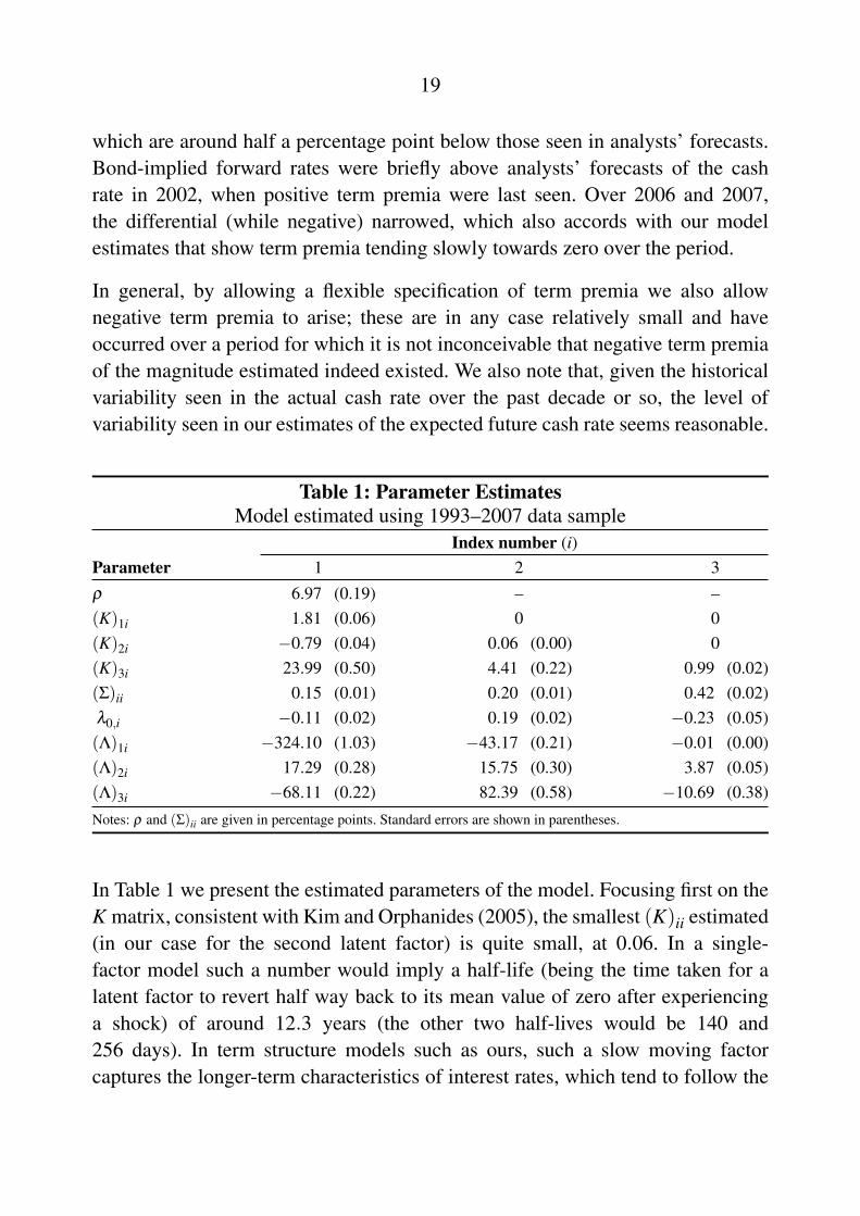
Table 1: Parameter EstimatesModel estimated using 1993–2007 data sample

Index number (i)Parameter 1 2 3ρ 6.97 (0.19) – –(K)1i 1.81 (0.06) 0 0(K)2i −0.79 (0.04) 0.06 (0.00) 0(K)3i 23.99 (0.50) 4.41 (0.22) 0.99 (0.02)(Σ)ii 0.15 (0.01) 0.20 (0.01) 0.42 (0.02)λ0,i −0.11 (0.02) 0.19 (0.02) −0.23 (0.05)(Λ)1i −324.10 (1.03) −43.17 (0.21) −0.01 (0.00)(Λ)2i 17.29 (0.28) 15.75 (0.30) 3.87 (0.05)(Λ)3i −68.11 (0.22) 82.39 (0.58) −10.69 (0.38)

Notes: ρ and (Σ)ii are given in percentage points. Standard errors are shown in parentheses.

In Table 1 we present the estimated parameters of the model. Focusing first on theK matrix, consistent with Kim and Orphanides (2005), the smallest (K)ii estimated(in our case for the second latent factor) is quite small, at 0.06. In a single-factor model such a number would imply a half-life (being the time taken for alatent factor to revert half way back to its mean value of zero after experiencinga shock) of around 12.3 years (the other two half-lives would be 140 and256 days). In term structure models such as ours, such a slow moving factorcaptures the longer-term characteristics of interest rates, which tend to follow the

20

business cycle or other gradual trends, and may not mean revert for many years.Such small diagonal entries of K will improve estimation of expected future shortrates at longer horizons. These estimated expectations would otherwise simply beflat and given by ρ .

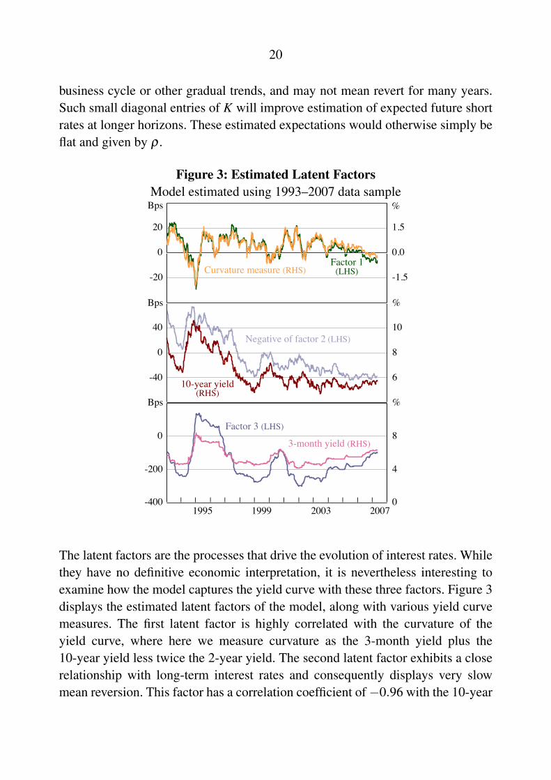
Figure 3: Estimated Latent FactorsModel estimated using 1993–2007 data sample

l l l l l l l l l l l l l l-400

-200

0

0

4

8

2007

-40

0

40

6

8

10

-20

0

20

-1.5

0.0

1.5

%

%

%

Bps

Bps

Bps

Factor 1(LHS)Curvature measure (RHS)

Negative of factor 2 (LHS)

10-year yield(RHS)

Factor 3 (LHS)

3-month yield (RHS)

200319991995

The latent factors are the processes that drive the evolution of interest rates. Whilethey have no definitive economic interpretation, it is nevertheless interesting toexamine how the model captures the yield curve with these three factors. Figure 3displays the estimated latent factors of the model, along with various yield curvemeasures. The first latent factor is highly correlated with the curvature of theyield curve, where here we measure curvature as the 3-month yield plus the10-year yield less twice the 2-year yield. The second latent factor exhibits a closerelationship with long-term interest rates and consequently displays very slowmean reversion. This factor has a correlation coefficient of−0.96 with the 10-year

21

yield. Finally, the third latent factor closely resembles short-term interest rates; ithas a correlation coefficient of 0.98 with the 3-month yield.

Interpreting the term premia parameters is much more difficult as there are moreof them and their effect on model outputs depends crucially on the sign and sizeof the xt latent factors. Hence it is probably more intuitive to focus on the termpremia produced (Figure 2) than on the actual numbers given in Table 1.

Finally the value of the constant ρ , which gives the short rate in steady-state andis estimated at 6.97 per cent, appears a little high. As mentioned earlier, it may bethat the model is placing the long-run equilibrium short rate at a higher level thanis warranted, thereby contributing to persistently negative term premia. The datasample does encompass the mid 1990s, formative years for the inflation-targetingregime and a period of relatively high cash rates which may have pushed up theestimate. Note also that our model gives the short rate at any time t as ρ plusthe sum of the latent factors at t, and while the latent factors decay to zero, thishappens very slowly. In fact over the sample period the value of x1,t + x2,t + x3,thas averaged −1.49 per cent. As the short rate is given by ρ + x1,t + x2,t + x3,t ,the equilibrium short rate over the sample could therefore be interpreted as beingcloser to 5½ per cent rather than to 7 per cent.

Actual and model-implied forward rates are shown in Figure 4. The fit is notperfect, but at any time the dynamic term structure model has much less flexibilityin generating yields along the curve than the model used to estimate the zero-coupon yields – it must rely on the three latent factor values to generate an entireyield curve. Hence we would not expect the model to be perfect. Rather, we trustthat it broadly characterises the observed actual yields, which appears to be thecase – model errors are generally small and hover around zero, only departingwhen yields rise or fall particularly quickly.

22

Figure 4: Forward Rates – Actual and ModelModel estimated using 1993–2007 data sample

l l l l l l l l l l l l l l-2

0

2

4

6

8

10

l l l l l l l l l l l l l l l l l l l l l l l l l l l l -2

0

2

4

6

8

10

Model error

2007

5 years ahead3 years ahead1 year ahead

Actual rate

Model impliedrate

19982007199820071998

%%

5.2 The Period 1997 to 2007

The data sample used in Section 5.1 spans the adoption by the Reserve Bank of the2 to 3 per cent inflation target, the decline in inflation expectations, and the formalacknowledgement of Reserve Bank independence. As a result, there may be astructural break for which the model does not account. To check the robustness ofthe results to this possibility we estimate the model again using a restricted samplewhich encompasses the more stable period from 1997 to early 2007. Although themodel estimates over this shorter sample are quite similar to those for the fullsample, it is interesting to compare the two.

The estimated expected future short rates and term premia are given in Figure 5.The most obvious difference between Figure 5 and Figure 2 is the more stableexpected future short rates and, consequently, the more variable term premia seenin the shorter sample. This is unlikely to be related to the K matrix since the shortersample has one latent factor which is even slower to mean revert than in the case ofthe longer sample. The term premia parameters Λ and λλλ 0 are numerically larger inthe short sample model indicating, all else equal, that changes in yields will have

23

a larger impact on term premia (and so a smaller impact on expected future shortrates) than in the longer sample.

Figure 5: Decomposition of the Forward RateModel estimated using 1997–2007 data sample

l l l l l l l l l l-2

0

2

4

6

8

l l l l l l l l l l l l l l l l l l l l -2

0

2

4

6

8

Term premium

2007

5 years ahead3 years ahead1 year ahead

Forward rate

Expectedfuture short rate

20012007200120072001

%%

In the shorter sample model there is an apparent upward trend in short rateexpectations from around 2004 or earlier. Again it is hard to determine exactlywhat caused this, but it did occur during a time of rising cash rates, low butrising inflation, falling unemployment and stable growth. So for the 1-year aheadforecast at least, the trend seems plausible. The trend in the 5-year ahead forecastis smaller but still apparent. However, being of the order of less than one-quarter ofa percentage point, it is probably not significant given the precision of the model .

Despite differences between the models one should keep in mind that the two areactually quite similar – the differences regard the degree of certain phenomena,not their existence. In fact, the estimates produced by the two models aregenerally within half a percentage point of each other; by comparison, Kim andOrphanides (2005), who also estimate models over two different sample periods,find differences in the order of around 2 percentage points.

24

The estimated parameters of the model over the short sample are given in Table 2.Similar to the longer sample, the smallest (K)ii estimated (in this case for thefirst latent factor) is small at 0.01. In a single-factor model such a number wouldimply a half-life of around 130 years (the other two half-lives would be 94 and459 days). The extremely slow mean reversion of the first latent factor is likelydue to the short sample period used, which spans a period of strong growth andlow inflation, and in particular does not span a ‘full’ economic cycle encompassinga sizeable economic downturn.

Table 2: Parameter EstimatesModel estimated using 1997–2007 data sample

Index number (i)Parameter 1 2 3ρ 6.78 (0.06) – –(K)1i 0.01 (0.00) 0 0(K)2i 0.55 (0.01) 2.69 (0.04) 0(K)3i 2.88 (0.05) 17.38 (0.11) 0.55 (0.01)(Σ)ii 0.08 (0.00) 0.15 (0.01) 0.30 (0.01)λ0,i 1.45 (0.01) −1.91 (0.03) −1.06 (0.02)(Λ)1i 465.20 (0.39) 440.07 (0.26) 12.81 (0.09)(Λ)2i −699.87 (0.44) −763.06 (0.48) 1.16 (0.03)(Λ)3i −171.60 (0.21) −396.64 (0.28) −109.58 (0.17)

Notes: ρ and (Σ)ii are given in percentage points. Standard errors are shown in parentheses.

Figure 6 shows that the first latent factor exhibits slow mean reversion, and is infact highly correlated with the slope of the yield curve (correlation coefficient of−0.97). In contrast, the much faster mean reverting third latent factor is highlycorrelated with the 3-month yield (correlation coefficient of 0.98), while thesecond latent factor is correlated with both the level and the curvature of yields.

It is interesting to note that for the shorter sample model, ρ is estimated at6.78 per cent, below the 6.97 per cent estimated for the longer sample model.As touched on earlier, the credibility of the Reserve Bank’s inflation target wasbeing tested around 1994, which resulted in interest rates, and especially long-termrates, rising quite strongly. There may therefore be a structural change in interestrate dynamics around 1995–1996, associated with the Reserve Bank’s success

25

Figure 6: Estimated Latent FactorsModel estimated using 1997-2007 data sample

l l l l l l l l l l-250

-200

-150

-100

-50

0

-250

-200

-150

-100

-50

0

Factor 2BpsBps

Factor 1

Factor 3

200720052003200119991997

in reducing inflation and the moderation in inflation expectations, for which themodel cannot account. The fact that the estimated equilibrium short rate is lowerover the shorter sample is consistent with this. The lower value of ρ also manifestsitself in less persistently negative term premia than those seen in the longer sample(note that similar to the longer sample model, the sum of latent factors averaged−1.56 per cent, giving an effective estimated short rate over the period of close to5¼ per cent).

As a final point, it is interesting to compare our term premia estimates with thosederived for US data. Figure 7 shows 1-, 3- and 5-year term premia as estimatedby us for Australian data, as well as corresponding term premia estimated by Kimand Wright (2005), who also use the Kim and Orphanides model, for US data.16

One can see that, excepting a level difference between the two series, the estimatedAustralian and US term premia track each other relatively closely – the correlationcoefficient between the two series is 0.84 for the 1-year ahead term premia, 0.90for the 3-year ahead term premia, and 0.81 for the 5-year ahead term premia. These

16 Available from http://www.federalreserve.gov/Pubs/feds/2005/200533/feds200533.xls.

26

Figure 7: Estimated Term Premia

l l l l l l l l l l-2

-1

0

1

2

3

l l l l l l l l l l l l l l l l l l l l -2

-1

0

1

2

3

2007

5 years ahead3 years ahead1 year ahead

Australia

US

20012007200120072001

%%

results suggest that term premia may be driven by global, as opposed to country-specific, phenomena, as typified for example by the global ‘search for yield’ thatreceived so much attention earlier this decade.

6. Conclusion

We have used data on coupon-bearing Australian Government bonds and OIS ratesto estimate risk-free zero-coupon yield and forward curves for Australia from 1992to 2007. These curves, and analysts’ forecasts of future interest rates, were thenused to fit an affine term structure model to Australian interest rates, with the aimof decomposing forward rates into expected future short rates and term premia.

The model produces plausible results, although given the complexity of the modeland the difficulty of calibrating it to the data, a false level of precision should not beattributed to the results. The results show a large and sustained fall in term premiafrom around 1996 to 2007, when inflation credibility became more entrenched andso inflation expectations declined. This period displays relatively low inflation,stable economic growth and stable bond yields.

27

The model suggests that there have been small negative term premia for someperiods. The finding of negative term premia has been a global phenomenon duringthe early to mid 2000s, as seen in the decline in long-term interest rates. This couldreflect the widely discussed ‘search for yield’ that occurred over this period, ormay be explained by an over-shooting of bond yields. In Australia’s case, therelatively low supply of government bonds, which has tended to fall over theperiod considered, may have contributed to negative term premia as risk-averseand mandate-constrained investors bid up the price of these bonds.

Notwithstanding the above discussion, the results seem to imply that expectedfuture short rates are relatively stable in Australia. The results also imply that,based on expectations of future monetary policy, yields on government bondshave been lower than might be expected, with term premia attached to these bondsconsequently being negative, at least towards the end of our sample period.

28

Appendix A: Zero-coupon Yields

We estimate zero-coupon yields using the Merrill Lynch Exponential Spline(MLES) methodology adapted from Li et al (2001). This technique appears tobe very efficient, and produces a good fit for the input data (technical details aregiven later in this Appendix).

The hardest data to fit is for maturities around the 1-year mark, where from early2001 the input data for any given day transitions from OIS rates (used as inputdata for maturities extending up to 1 year into the future) to bond yields (used formaturities greater than or equal to 18 months into the future). Although we regardOIS rates as the closest available substitute for risk-free Treasury note yields, theyare not Treasury notes – they are swap contracts as opposed to physical bonds ornotes, and they trade in a different market to physical bonds or notes, which maymean that the factors affecting OIS pricing are sometimes different from thoseaffecting note or bond pricing. That being said, the MLES procedure still providesa good fit to the data even here – the average absolute error between the 1-year OISyield and the MLES estimated 1-year yield is around 3½ basis points; the largesterror is only 12 basis points and the error is larger than 10 basis points only threetimes. Taking a broader perspective, the fit of the MLES method is in fact verygood, with the daily mean absolute error between fitted yields and actual yieldsaveraging less than 2 basis points, and peaking at only 6 basis points.

Another potential and related criticism is the mixing together of OIS and bondyields to estimate a single yield curve. We believe that although Treasury noteyields would be preferable for short maturity data inputs, in their absence, OISrates are the next best, and in fact a very good, substitute. They are virtually risk-free and so can sensibly be used in the estimation of our risk-free yield curve, andthey fulfil a vital function in supplying information about the short end of the yieldcurve that would otherwise be unavailable.

In any case, given that we are fitting a flexible term structure model, so long as theevolution of OIS yields through time is comparable to the evolution of Treasurynote or bond yields, any residual risk premia inherent in OIS yields should becaptured as short-dated term premia in the model. Overall, while Treasury noteyields would be preferable, in their absence OIS yields provide a very goodsubstitute.

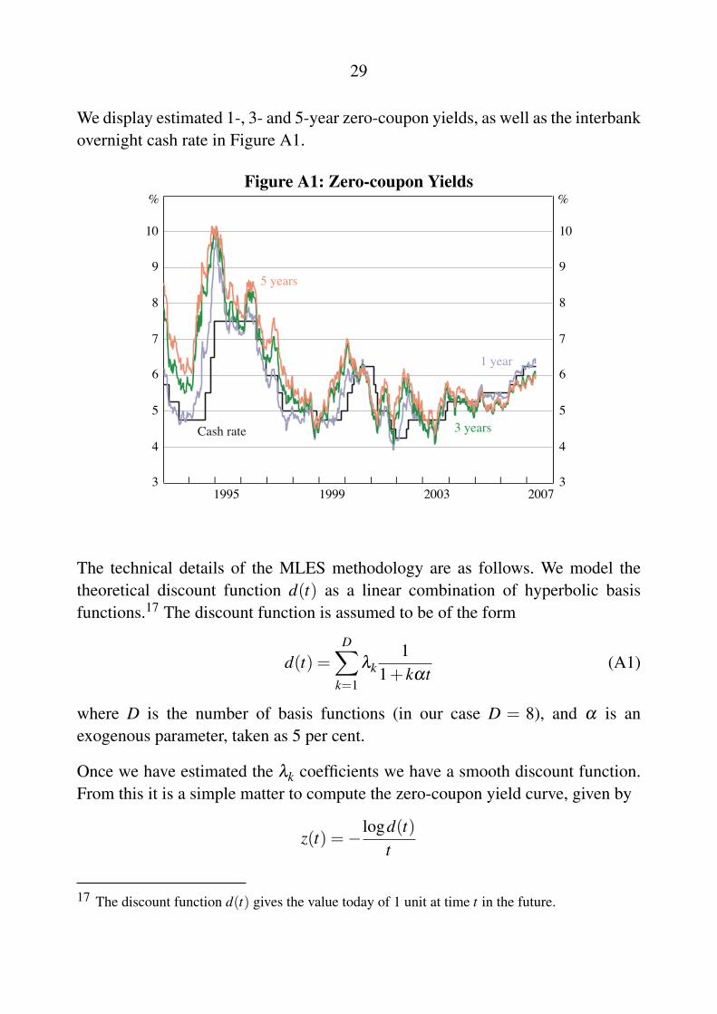
29

We display estimated 1-, 3- and 5-year zero-coupon yields, as well as the interbankovernight cash rate in Figure A1.

Figure A1: Zero-coupon Yields

l l l l l l l l l l l l l l3

4

5

6

7

8

9

10

3

4

5

6

7

8

9

10

1 year

2007

%%

200319991995

5 years

3 yearsCash rate

The technical details of the MLES methodology are as follows. We model thetheoretical discount function d(t) as a linear combination of hyperbolic basisfunctions.17 The discount function is assumed to be of the form

d(t) =D∑

k=1

λk1

1+ kαt(A1)

where D is the number of basis functions (in our case D = 8), and α is anexogenous parameter, taken as 5 per cent.

Once we have estimated the λk coefficients we have a smooth discount function.From this it is a simple matter to compute the zero-coupon yield curve, given by

z(t) =−logd(t)t

17 The discount function d(t) gives the value today of 1 unit at time t in the future.

30

and the (instantaneous) forward curve given by

f (t) = z(t)+ tz′(t).

Given the assumed form of the discount function, the theoretical price of bond i isgiven by

Bi =mi∑j=1

ci jd(τi j)

where ci j is the jth cash flow of bond i, occurring at time τi j, and mi is the numberof cash flows belonging to bond i. That is, the price of bond i is the sum of itsdiscounted cash flows.

The price of a bond is the linear sum of its discounted cash flows. The discountfunction is assumed to be a linear sum of basis functions. This linearity allows usto write the vector of bond prices or OIS rates B as

B = Xβββ + εεε (A2)

where BT = [B1, · · · ,Bn] is the vector of observed prices,18 X is a n×D matrixwith Xik =

∑mij=1 ci j

11+kατi j

, βββ = (λ1, · · · ,λD)T and εεε a vector of errors.

For W the weight matrix,19 if we wished to minimise the weighted squared pricingerrors εεε

TWεεε , then the solution would be given by

βββ = (XTWX)−1XTWB. (A3)

We wish to impose some restrictions on d(t) however: d(0), the discount rate att = 0 should be 1, that is, one dollar today is worth one dollar. Also, the cashrate (as of today) is known and fixed, and so should be reflected in the discountfunction. These requirements complicate matters slightly.

From Equation (A1) it is clear that d(0) =∑D

k=1 λk. Hence requiring d(0) = 1 isequivalent to requiring λD = 1−

∑D−1k=1 λk.

18 For OIS contracts the ‘observed price’ corresponds to the price of a discount security payingthe OIS yield.

19 The weight attached to each bond is taken as its inverse duration. This has the effect ofminimising fitted yield errors, as opposed to price errors.

31

Writing fk(t) = 11+kαt , we can ensure that the 1-day yield is given by the overnight

cash rate, r say, by requiring

d(1

365) =

D∑k=1

λk fk(1

365) =

11+ 1

365r

100. (A4)

Writing y = (1 + 1365

r100)

−1, from Equation (A4) these two constraints areequivalent to

y = λ1 f1(1

365)+ · · ·+λD−1 fD−1(

1365

)+(1−D−1∑k=1

λk) fD(1

365)

= λ1( f1(1

365)− fD(

1365

))+ · · ·+λD−1( fD−1(1

365)− fD(

1365

))+ fD(1

365)

and hence

λD−1 =y− fD( 1

365)

fD−1(1

365)− fD( 1365)− (λ1

f1(1

365)− fD( 1365)

fD−1(1

365)− fD( 1365)

+ · · ·

+λD−2fD−2(

1365)− fD( 1

365)

fD−1(1

365)− fD( 1365)

)

= λ∗D−1 (A5)

We first impose the d(0) = 1 constraint. Writing xi for the ith column of the Xmatrix, Equation (A2) becomes

B = x1λ1 + · · ·+xD−1λD−1 +xDλD + εεε

= x1λ1 + · · ·+xD−1λD−1 +xD(1−D−1∑k=1

λk)+ εεε

so thatB−xD = (x1−xD)λ1 + · · ·+(xD−1−xD)λD−1 + εεε. (A6)

Writing B = B− xD, xi = xi− xD, X = (x1, · · · , xD−1) and βββ = (λ1, · · · ,λD−1)T ,

Equation (A6) becomesB = X βββ + εεε. (A7)

32

The estimate of βββ which minimises εεεTWεεε is (XTWX)−1XTW B. Hence we have

found the least squares estimate of βββ from Equation (A2), subject to the d(0) = 1constraint.

If we now start from Equation (A7), replace λD−1 with λ∗D−1 from Equation (A5)

and follow the procedure above, we obtain our estimator. In this case the estimatorof βββ = (λ1, · · · ,λD−2)

T which solves

B = X βββ + εεε (A8)

for B = B − y− fD( 1365)

fD−1(1

365)− fD( 1365)

xD−1 and X = (x1, · · · , xD−2) for

xi = xi−fi(

1365)− fD( 1

365)fD−1(

1365)− fD( 1

365)xD−1 is given by

βββ = (XTWX)−1XTW B. (A9)

Hence we have solved Equation (A2) subject to both desired constraints.

33

Appendix B: Risk-neutral Bond Pricing

Here we examine why bonds should be priced under the risk-neutral measure. Tosimplify the analysis we work with a single factor model, that is

rt = ρ + xt (B1)dxt =−kxtdt +σdWt (B2)λt = λ0 +λ1xt (B3)

where all variables are scalars.

Consider the probability space (Ω,F ,P) with associated filtration Ft taken as theaugmented filtration of σWs|s ≤ t (see, for example, Steele 2001). Xt is an Itoprocess if

dXt = µxdt +σxdWt

for µx and σx adapted to Ft . Ito’s lemma then states that for any function F(x, t)such that F is twice differentiable in x and differentiable in t,

dF =

(∂F∂ t

+ µx∂F∂x

+12

σ2x

∂2F

∂x2

)dt +σx

∂F∂x

dWt .

Applying Ito’s lemma to Equation (B1) we trivially get

drt =−kxtdt +σdWt

≡ µrdt +σrdWt .

Now let PA(rt , t) and PB(rt , t) denote the time t price of two zero-coupon bondswith different maturity dates. Then by Ito’s lemma, Pi (i = A, B) will satisfy

dPi =

(∂Pi

∂ t+ µr

∂Pi

∂ r+

12

σ2r

∂2Pi

∂ r2

)dt +σr

∂Pi

∂ rdWt (B4)

≡ µidt +σ

idWt . (B5)

Consider a portfolio that is long one A bond and short h B bonds. At time t thisportfolio has value

Vt = PA−hPB. (B6)

34

If held for dt, the portfolio’s value changes by

dVt = dPA−hdPB

= (µA−hµ

B)dt +(σA−hσB)dWt . (B7)

Hence we can make the portfolio instantaneously riskless by choosing h = σA/σ

B.In this case, the portfolio must earn the risk-free rate rt and so

dVt = rtVtdt. (B8)

Substituting Equations (B6) and (B7) into Equation (B8) and setting h = σA/σ

B

leads to

µA− σ

A

σB µ

B = rt(PA− σ

A

σB PB)

orµ

A− rtPA

σA =

µB− rtP

B

σB .

Hence the ratio (µ − rtP)/σ is independent of the choice of bond, and so theremust exist a function λr such that

µ− rtPσ

= λr (B9)

holds for any bond price P.

Now substituting µ and σ as identified by Equations (B4) and (B5) intoEquation (B9) results in a Black-Scholes type partial differential equation

∂P∂ t

= rtP− (µr−λrσr)∂P∂ r− 1

2σ

2r

∂2P

∂ r2 (B10)

which is solved subject to appropriate boundary conditions (bonds pay 1 unit atmaturity) and the radiation condition P→ 0 as r→ ∞.

The Feynman-Kac formula then says that the solution to Equation (B10) is givenby

Pt,τ = E∗t[

exp(−ˆ T

trsds)

]where rt satisfies

drt = (µr−λrσr)dt +σrdW ∗t ; dW ∗t = dWt +λrdt

and W ∗t is standard Brownian motion in the risk-neutral measure associated withE∗.

35

Appendix C: Model Implementation

C.1 Formulas for aτ and bτ

From Kim and Orphanides (2005) we take the following formulas (withcorrections):

aτ =1τ

((K∗µµµ∗)′(M1,τ − τI)K∗−1′1

−12

1′K∗−1(M2,τ −ΣΣ′M1,τ −M′1,τΣΣ

′+ τΣΣ′)K∗−1′1+ τρ

)bτ =

1τ

M1,τ1

where

M1,τ =−K∗−1′(

e−K∗′τ − I

)M2,τ =−vec−1

(((K∗⊗ I)+(I⊗K∗))−1vec

(e−K∗τ

ΣΣ′e−K∗

′τ −ΣΣ

′))

with K∗ = K +ΣΛ, µµµ∗ = K∗−1

Σλλλ 0, vec taking a matrix to a vector column-wise,and vec−1 doing the opposite.

C.2 The Kalman Filter

Our implementation of the Kalman filter is based on that used by Duffee andStanton (2004). The recursion goes from t = 1 forward, and is as follows:

1. Using the current value of xt , compute the one-step-ahead forecast of xt , givenby xt+1|t = e−Khxt , and its variance matrix Pt+1|t = e−KhPt|t(e

−Kh)′+Ωh.

2. Compute the one-step-ahead forecast of yt , given by yt+1|t = a + Bxt+1|t , andits variance matrix Vt+1|t = BPt+1|tB

′+ R, where R is the zero-coupon bondmeasurement error variance matrix.

3. Compute the forecast errors of yt+1|t , given by et+1 = yt+1−yt+1|t .

4. Update the prediction of xt+1 with xt+1|t+1 = xt+1|t +Pt+1|tB′V−1

t+1|tet+1 and the

variance with Pt+1|t+1 = Pt+1|t−Pt+1|tB′V−1

t+1|tBPt+1|t .

36

For times t when we have analysts’ forecasts, replace yt , a, B and R by yt , a, Band R, respectively.

We then choose our parameter vector Θ to solve

Θ∗ =

argmaxΘ

n∑t=1

LL(et ,Vt|t−1)

where the sample is n periods long, and the period-t approximate log-likelihood isgiven by

LL(et ,Vt|t−1) =−12

(log |Vt|t−1|+ et

′V−1t|t−1et

).

C.3 Implementation

To implement the model we restrict the parameters to those which result in K andK∗ having positive eigenvalues. This results in e−Ks→ 0 and e−K∗s→ 0 as s→∞,which ensures the stability of the model (see Equation (9) and the formulas for aτ

and bτ). We also require that the σi, being variances, are positive.

By way of parameter choices that must be made, we set x1 = [0.005, 0.03, 0.01]′

(with an initial standard deviation of 10 per cent) and then discard the firstsix months of the estimation. The standard deviation of zero-coupon yieldmeasurement errors is set to 10 basis points, while those of the survey forecastsare set to 50 basis points per square root year.

Finally, the standard errors in Tables 1 and 2 are calculated using a random walkchain Metropolis-Hastings algorithm – for details see Geweke (1992).

37

References

Beechey M (2004), ‘Excess Sensitivity and Volatility of Long Interest Rates: TheRole of Limited Information in Bond Markets’, Sveriges Riksbank Working PaperNo 173.

Bolder DJ and S Gusba (2002), ‘Exponentials, Polynomials, and Fourier Series:More Yield Curve Modelling at the Bank of Canada’, Bank of Canada WorkingPaper No 02-29.

Cochrane JH (2001), Asset Pricing, Princeton University Press, Princeton.

Dai Q and KJ Singleton (2002), ‘Expectation Puzzles, Time-Varying RiskPremia, and Affine Models of the Term Structure’, Journal of FinancialEconomics, 63(3), pp 415–441.

de Jong F (2000), ‘Time Series and Cross-Section Information in Affine Term-Structure Models’, Journal of Business & Economic Statistics, 18(3), pp 300–314.

Duffee GR (2002), ‘Term Premia and Interest Rate Forecasts in Affine Models’,Journal of Finance, 57(1), pp 405–443.

Duffee GR and RH Stanton (2004), ‘Estimation of Dynamic Term StructureModels’, unpublished, Hass School of Business, UC Berkeley.

Duffie D and R Kan (1996), ‘A Yield-Factor Model of Interest Rates’,Mathematical Finance, 6(4), pp 379–406.

Geweke J (1992), ‘Evaluating the Accuracy of Sampling-Based Approaches tothe Calculation of Posterior Moments’, in JO Berger, JM Bernardo, AP Dawidand AFM Smith (eds), Proceedings of the Fourth Valencia International Meetingon Bayesian Statistics, Oxford University Press, Oxford, pp 169–194.

Gürkaynak RS, BP Sack and ET Swanson (2003), ‘The Excess Sensitivityof Long-Term Interest Rates: Evidence and Implications for MacroeconomicModels’, Federal Reserve Board Finance and Economics Discussion SeriesNo 2003-50.

Kim DH and A Orphanides (2005), ‘Term Structure Estimation with SurveyData on Interest Rate Forecasts’, Federal Reserve Board Finance and EconomicsDiscussion Series No 2005-48.

38

Kim DH and JH Wright (2005), ‘An Arbitrage-Free Three-Factor TermStructure Model and the Recent Behavior of Long-Term Yields and Distant-Horizon Forward Rates’, Federal Reserve Board Finance and EconomicsDiscussion Series No 2005-33.

Kremer M and M Rostagno (2006), ‘The Long-Term Interest Rate Conundrumin the Euro Area: Potential Explanations and Implications for Monetary Policy’,paper presented at the BIS Autumn Meeting of Central Bank Economists on‘Understanding Asset Prices: Determinants and Policy Implications’, Basel, 30–31 October.

Li B, E DeWetering, G Lucas, R Brenner and A Shapiro (2001), ‘Merrill LynchExponential Spline Model’, Merrill Lynch Working Paper.

Reserve Bank of Australia (RBA) (2002), ‘Overnight Indexed Swap Rates’,Reserve Bank of Australia Bulletin, pp 22–25.

Rudebusch GD, BP Sack and ET Swanson (2007), ‘MacroeconomicImplications of Changes in the Term Premium’, Federal Reserve Bank of St. LouisReview, 89(4), pp 241–269.

Rudebusch GD and T Wu (2008), ‘A Macro-Finance Model of the TermStructure, Monetary Policy and the Economy’, Economic Journal, 118(530),pp 906–926.

Steele JM (2001), Stochastic Calculus and Financial Applications, Springer, NewYork.

Swanson ET (2007), ‘What We Do and Don’t Know about the Term Premium’,Federal Reserve Board of San Francisco Economic Letter No 2007-21.

Westaway P (2006), ‘Extracting Information from Financial Markets at theBank of England: Refining the Modelling Toolkit and Strengthening theTheoretical Underpinnings’, paper presented at the BIS Autumn Meeting ofCentral Bank Economists on ‘Understanding Asset Prices: Determinants andPolicy Implications’, Basel, 30–31 October.