Finance and Economics Discussion SeriesDivisions of Research & Statistics and Monetary Affairs

Federal Reserve Board, Washington, D.C.

Banking panics and deflation in dynamic general equilibrium

Francesca Carapella

2015-018

Please cite this paper as:Carapella, Francesca (2015). “Banking panics and deflation in dynamic general equilib-rium,” Finance and Economics Discussion Series 2015-018. Washington: Board of Governorsof the Federal Reserve System, http://dx.doi.org/10.17016/FEDS.2015.018.

NOTE: Staff working papers in the Finance and Economics Discussion Series (FEDS) are preliminarymaterials circulated to stimulate discussion and critical comment. The analysis and conclusions set forthare those of the authors and do not indicate concurrence by other members of the research staff or theBoard of Governors. References in publications to the Finance and Economics Discussion Series (other thanacknowledgement) should be cleared with the author(s) to protect the tentative character of these papers.

Banking panics and deflation in dynamic general equilibrium∗

Francesca Carapella†

Federal Reserve Board

August 2012

Abstract

This paper develops a framework to study the interaction between banking, price dynam-ics, and monetary policy. Deposit contracts are written in nominal terms: if prices unex-pectedly fall, the real value of banks’ existing obligations increases. Banks default, panicsprecipitate, economic activity declines. If banks default, aggregate demand for cash increasesbecause financial intermediation provided by banks disappears. When money supply isun-changed, the price level drops, thereby providing incentives for banks to default. Activemonetary policy prevents banks from failing and output from falling. Deposit insurance canachieve the same goal but amplifies business cycle fluctuations by inducing moral hazard.

JEL: E53, E58, G21, N12. Keywords: banking panics, deflation, deposit insurance.

1 Introduction

Every major banking crisis in the United States between 1837 and 1933 was accompanied

by declines in prices and downturns in economic activity. In particular, during 1930-33 the

U.S. financial system witnessed waves of bank failures and a protracted decline in output1.

During the 1990s Japan had a similar experience: prices continuously fell, banks had trou-

bles surviving, and output stalled2. In the United States during the recent financial crisis,

several hundred banks were closed between 2007 and 2010, some large investment banks

and mutual/hedge funds failed or were severely troubled, and despite massive interven-

tions by the Federal Reserve, prices declined in the third and fourth quarters of 2008 amid

concerns about further deflation from policy makers3. These events give rise to several

∗I am very grateful to V.V Chari, Larry Jones and Warren Weber for their advice and encouragement. Ialso thank Laurence Ales,Roozbeh Hosseini, Tim Kehoe, Pricila Maziero, Ellen McGrattan, Chris Phelan,Monika Piazzesi, Facundo Piguillem, Martin Schneider, Gerhard Sorger, participants at the 2007 MidwestMacro conference in Cleveland, the 2008 SED meeting in Prague, the 2008 Vienna Macro workshop, 2009ESSIM in Chateau de Ragny for comments and suggestions.†The opinions are the authors’ and do not necessarily reflect those of the Federal Reserve Board.

Contact: Francesca.Carapella@frb.gov. Federal Reserve Board of Governors, Washington DC, 20551.1See Table A.1, Appendix A.12See graph 5, Appendix A.23See graph 6, Appendix A.3

1

questions: what is the connection between banks and price declines? May bank failures

and deflation naturally occur together? Can monetary policy help prevent banking failures,

or does deposit insurance suffice? This paper provides answers to these questions.

Economists have long regarded disruptions in the financial sector as a source of economic

fluctuations ([19], [2], [4]). The key mechanism works through an increase in the cost

of intermediation during a financial crisis: the increased cost causes a decline in credit,

which can ultimately lead to periods of low growth and recession. One explanation for the

observed protracted decline in output during a financial crisis is that small shocks may be

amplified and propagated throughout the financial system and the rest of the economy:

this paper provides one such explanation. It describes a novel amplification mechanism

of banking crisis and analyzes policy responses that can prevent such amplification from

being triggered.

In the model, bank failures are amplified by deflation and at the same time feed back

deflation, in a vicious circle4. A key friction is that repayments on deposits are fixed

in nominal terms, rather than contingent on the realization of prices. Because of this,

banks face a mismatch in their balance sheets between the value of their assets (productive

projects in which they invest, and loans to firms) and liabilities (deposits). Deposits are at

book value because they are indexed to the price level at the time the liability originated,

that is, when the deposit contract was signed. Banks’ productive projects are valued at

current market prices. If prices unexpectedly fall, then the real value of existing nominal

obligations increases, but the real value of assets is unchanged5: when the decline in prices

is large enough, it leads banks to fail (figure 1, right-hand side). When banks fail, depositors

drastically reduce deposit holdings and increase cash holdings: a banking panic occurs6.

The other key and novel ingredient in the model is that banks provide financial in-

termediation to households by issuing liabilities that can be used as means of payment

4Deflation is not a necessary condition for the amplification mechanism described in the model: bankingcrisis may be amplified even by an inflation rate lower than anticipated.

5This is equivalent to banks making nominal loans to firms. When the price level falls, firms default ontheir loans because the real value of their nominal liabilities increases, but the real value of assets (outputfrom productive projects) is unchanged. Therefore when firms default on their loans, banks’ assets are justthe collateral on the loans, valued at current prices.

6Contrary to the mechanism at work in Diamond and Dybvig [15] models, the reason banks fail in thismodel is not a combination of a coordination failure on the side of depositors and a maturity mismatch inbanks’ balance sheets. In this model a banking panic occurs when depositors who hold maturing claims atthe bank are not paid and do not renew their deposits. The panic is precipitated because depositors expectbanks to fail and because banks face a mismatch between nominal liabilities and real assets rather than amaturity mismatch.

2

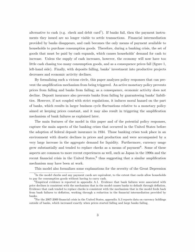
alternative to cash (e.g. check and debit card7). If banks fail, then the payment instru-

ments they issued are no longer viable to settle transactions. Financial intermediation

provided by banks disappears, and cash becomes the only means of payment available to

households to purchase consumption goods. Therefore, during a banking crisis, the set of

goods that must be paid by cash expands, which causes households’ demand for cash to

increase. Unless the supply of cash increases, however, the economy will now have too

little cash chasing too many consumption goods, and as a consequence prices fall (figure 1,

left-hand side). Finally, with deposits falling, banks’ investment into productive projects

decreases and economic activity declines.

By formalizing such a vicious circle, this paper analyzes policy responses that can pre-

vent the amplification mechanism from being triggered. An active monetary policy prevents

prices from falling and banks from failing; as a consequence, economic activity does not

decline. Deposit insurance also prevents banks from failing by guaranteeing banks’ liabili-

ties. However, if not coupled with strict regulations, it induces moral hazard on the part

of banks, which results in larger business cycle fluctuations relative to a monetary policy

aimed at keeping prices constant, and it may also result in triggering the amplification

mechanism of bank failures as explained later.

The main features of the model in this paper and of the potential policy responses,

capture the main aspects of the banking crises that occurred in the United States before

the adoption of federal deposit insurance in 1934. Those banking crises took place in an

environment with drastic declines in prices and production and were accompanied by a

very large increase in the aggregate demand for liquidity. Furthermore, currency usage

grew substantially and tended to replace checks as a means of payment8. Some of these

aspects are common to more recent experiences as well, such as Japan in the 1990s and the

recent financial crisis in the United States,9 thus suggesting that a similar amplification

mechanism may have been at work.

This model also formalizes some explanations for the severity of the Great Depression

7In the model checks and any payment cards are equivalent, to the extent that cards allow householdsto pay for consumption goods without having to carry cash.

8Empirical evidence is reported in appendix A.1. Evidence that bank failures were associated withprice declines is consistent with the mechanism that in the model causes banks to default through deflation.Evidence that cash tended to replace checks is consistent with the mechanism that in the model feeds backfrom bank failures to deflation, working through a reduction in the financial intermediation provided bybanks.

9For the 2007-2009 financial crisis in the United States, appendix A.3 reports data on currency holdingsoutside of banks, which increased exactly when prices started falling and large banks failing.

3

and provides support for some policy recommendations that followed it. Irving Fisher’s

[18] debt-deflation theory of the Great Depression identifies the unanticipated fall in the

price level and consequent increase in the real amount of debt as the cause of the depression

continuing in a vicious spiral. Fisher’s theory also identifies a policy response: reflating

the price level up to the average level at which outstanding debts were contracted and

maintaining that level unchanged10.

Friedman and Schwartz [19] and Warburton [27], [28], [29] share a similar view of the

role of monetary policy in relieving the severity of the contraction. Friedman and Schwartz

[19] see the banking and liquidity crisis as responsible for the decline in the stock of money

which, in turn, caused prices to fall11 and eventually led to the collapse of the banking

system. They hypothesize that prevention or moderation of the decline in the stock of

money would have reduced the contraction’s severity and its duration.

This paper formalizes Friedman and Schwartz’s [19] hypothesis: monetary intervention

plays a useful role by adjusting the supply of liquidity to prevent prices from falling. This

paper also evaluates Friedman and Schwartz’s hypothesis relative to deposit insurance,

which was established at the federal level in the United States as a response to the fail-

ure of monetary authorities to avoid the collapse of the banking system during the early

1930s12. It is particularly relevant to this model that deposit insurance causes larger busi-

ness cycle fluctuations than a monetary policy a la Friedman and Schwartz, because the

fluctuations may trigger the amplification mechanism of banking failures described above.

Larger output fluctuations cause banks to fail more often, in bad states of the world. If it

is not feasible for deposit insurance to guarantee that payments made by checks and cards

issued by failed banks are honored in every state of the world, then bank failures cause a

reduction in banks’ provision of payment services and an increase in the demand for cash,

which results in a fall in prices. The vicious circle of banking failures and deflation is thus

triggered.

It is crucial in this model that the amplification mechanism of the banking crisis works

exclusively through the unanticipated fall in prices: once that is prevented no amplification

is triggered. This has important implications for policy because in most banking-panic

models13 a panic is the outcome of a coordination failure among depositors: fearing that

10Fisher [18], pg. 34611Friedman and Schwartz (pp.351) argue that the failures were the mechanism through which a drastic

decline was produced in the stock of money. Absent any policy intervention, prices fell.12See Friedman and Schwartz [19] pp.300−, 420−.13This is a large literature that follows Diamond and Dybvig [15]; among many [17], [24].

4

other depositors’ withdrawals will cause the bank to become insolvent, depositors with no

urge to consume (patient depositors) run on the bank. In this paper, no coordination failure

among depositors occurs, and therefore deposit insurance has no purpose in guaranteeing

sufficient assets at the bank to cover withdrawals by patient depositors and avoid a panic.

In this paper, anything that causes a reduction in the financial intermediation provided by

banks will induce a fall in prices, which, in turn, puts pressure on the balance sheets of

banks that had survived, causing them to fail, so the economy moves along Fisher’s [18]

vicious spiral. The type of shock that triggers the spiral is irrelevant for the amplification

mechanism to be set in motion. A stock market crash or a large loss would reduce the

value of banks’ assets relative of existing nominal obligations and can trigger the circle.

A sunspot can trigger the mechanism as well by selecting the strategies to be played in

equilibrium. As soon as banks fail or prices exogenously fall, the amplification mechanism

is triggered. Hence, this paper provides a theory of how bank failures are propagated to

the real economy rather than a theory of banking panics.

Figure 1: Economic Mechanism

Price level falls

casht c

Mp =

Deposit contractsnominal Assets

real

(Banks’ liabilities)

Banks Default

Real assets < tp

1 nominal debt

Disruption of payment system

(more goods bought with

cash)

New loans fall, Output falls

It is also crucial that deposit contracts not be contingent on the realization of prices at

the time the repayment is due for the mismatch in banks’ balance sheet to arise. Diamond

and Rajan [16] study economies in which repayment on deposits is fixed over the next

5

instant, and compare the effects of a shock to the timing of banks’ production in environ-

ments with real versus nominal deposit contracts. They show that, under some conditions,

nominal deposits may exacerbate real liquidity shortages by increasing aggregate real liq-

uidity demand when supply falls, as in Fisher’s [18] debt-deflation argument. So they focus

on the right-hand side of the circle in Figure 1.

This paper completes the circle, showing that banking failures and deflation may natu-

rally occur together and are mutually reinforcing. Diamond and Rajan [16] focus on how a

specific friction, nominal deposits, amplifies a shock to the timing of banks’ production, but

in their model there is nothing specific to the operation of the banking system that ampli-

fies liquidity shortages. Their amplification is purely the result of the interaction between

nominal deposits with fixed repayment over the next instant and a maturity mismatch in

banks’ balance sheets.

This paper introduces a role for banks in the amplification mechanism itself: banks

provide financial intermediation by issuing liabilities that can be used as means of payment.

When such intermediation disappears, aggregate liquidity demand increases, leading prices

to fall. Accounting for such feedback effect from bank failures to price dynamics is relevant

for two reasons. First, no real shock to banks’ balance sheets or output, or the timing

of production, is necessary to trigger the amplification, although such a shock would be

sufficient to trigger the amplification. Second, consider an economy in which banks play no

role in providing payment services but still issue nominal deposits with fixed repayments

over the next instant, as in Diamond and Rajan [16]. In such an economy, a drop in output

would require a shock of much greater magnitude than would be required in the economy

this paper describes, in which once a small shock forces a few banks to fail, the feedback

effect on prices causes more banks to fail, and so on with further effects on prices, in a

vicious circle.

The paper is organized as follows: section 2 sets up a static version of the full model

environment described in section 3, and derives the main result that banking failures and

deflation may naturally occur together and are mutually reinforcing. The full dynamic

model in section 3 also provides policy implications, after which section 4 concludes.

2 One period model

Consider an economy with a continuum of identical households and identical banks, each

represented by a Lebesgue measure on the interval [0, 1]. Households and banks move

6

simultaneously and they live only for one period. There are three consumption goods: a

cash good, a credit good and coconut. Coconut is used as numeraire14, cash goods can be

purchased only using coconut and credit goods can be purchased either with coconut, like

cash goods, or with credit. However, regardless of how credit goods are paid for, they are

intrinsically different consumption goods from cash goods.

Households’ preferences are represented by the utility function U : R3+ → R defined

over cash good, credit good and coconut: U(c1, c2, A′) = log c1 + log c2 + logA′, where

c1 denotes the consumption of cash good, c2 the consumption of credit good and A′ the

consumption of coconut.

Banks’ preferences are represented by the utility function V : R2+ → R defined over

cash and credit goods: V (cb1, cb2) = cb1 + cb2, where cb1 and cb2 denote banks’ consumption of

cash good and credit good respectively15.

At the beginning of the period banks are endowed with f units of labor. Households are

endowed with y units of labor, A units of coconut, and R claims denominated in coconut

on each bank that mature at the end of the period16. These are claims either payable with

coconut or with bank-issue liabilities, as will be explained later.

Households have access to three technologies: they can transform a unit of labor into

a unit of either cash or credit good17, they can carry coconut within the period, and they

can plant coconut at the beginning of the period18, which yields r > 1 per unit planted,

at the end of the period. Banks can transform a unit of labor into a unit of either cash

or credit good. The financial and productive sectors are consolidated in this economy and

represented by banks: this is without loss of generality since the crucial assumption is

that some agents face a mismatch in the denomination of assets and liabilities, here real

assets and nominal liabilities. If banks make nominal loans to firms then firms face such

14In a static model commodity money relative to fiat money solves the issue of agents not being willingto hold a good without intrinsic value (fiat money) until the end of the period. With preferences definedalso over coconut, agents accept coconut for payment and eat it at the end of the period.

15It is irrelevant for the results whether banks’ preferences are defined over cash good, credit good andcoconut like households, or as above. Defining preferences over coconut is useful in a static model becauseit makes agents willing to accept it for payment. In this setup banks pay households using the coconutthey have at the end of the period and offsetting with other banks any households’ remaining claims andobligations. If banks’ preferences were also defined over coconut then they could eat the coconut and payhouseholds just by offsetting with other banks their claims and obligations, as explained later.

16In this static version of the model, households’ endowment of R claims on banks play a key role inbanks’ default decision: they are equivalent to deposits fixed in nominal terms over the next instant in adynamic model.

17As in Lucas-Stokey [23]18In this static version of the model planting coconut is equivalent to depositing money at the bank.

7

a mismatch: every result in the paper maintains under the assumption that when firms’

default on the loans granted by banks, the best a bank can do it to seize the collateral (the

real assets of firms). This alternative version of the model is described in a separate online

appendix19.

2.1 Households’ problem

Similarly to Lucas-Stokey [23] each household is divided into a worker and a shopper: at

the beginning of the period the asset market opens and the worker and the shopper make

their portfolio decisions together, as a household. Households start the period with an

endowment of coconut (A) and decide how much of it to carry within the period (M) and

how much to plant (D), which returns r per unit of coconut planted at the end of the

period. Banks issue checkbooks, debit and credit cards to households at the beginning

of the period against the value of households’ income at the end of the period which is

directly deposited at the bank. So households can write checks and use debit and credit

cards to transfer balances from their account at the bank to other households and banks.

Therefore, at the beginning of the period households face a securities market constraint:

M +D ≤ A. Then the goods’ market opens and the worker and the shopper are separated

from each other: the shopper takes the coconut that was not planted (M) and visits

other households and banks to purchase consumption goods. The shopper is constrained

to purchase cash goods by paying right away using coconut, whereas she can purchase

credit goods by paying right away either with coconut or using checks and cards issued by

banks20.

19This appendix is available at http://sites.google.com/site/carapellaf/research20In the model credit and debit cards are equivalent as means of payment alternative to cash: they

differ only relative to the friction introduced between securities and goods markets. If we assume that thereis a timing friction between the instant when income is earned by the worker and the instant when theconsumption purchase is made by the shopper, then banks are actually extending credit to households forthe time elapsed between the consumption purchase and the receipt of income. So credit goods paymentsare done by credit cards.However if we assume that the friction is only physical separation between the shopper and the worker, sothat the worker earns income at the same time as the shopper buys consumption goods, but the income isdeposited automatically in an account that the household has with a bank, then credit goods payment aredone by debit cards, since no credit is extended to the household. In this case, a debit card makes resourcesthat are available in household’s portfolios, also available to the physical location where they are needed,that is to say with the shopper.Because credit and debit cards payments are equivalent in this model, for simplicity they will be referred toas credit payments, as the goods that can be purchased by credit and debit cards are referred to as creditgoods.

8

Her income at the end of the period is given by the return on the coconut planted at

the beginning of the period, (rD), the claims on banks (R) and the income from selling

goods produced with his endowment of labor (py, where p is the price level).

When households pay for credit goods purchases using checks or cards, they have

no remaining obligation: banks are responsible to settle those payments21. Banks settle

payments at the end of the period by netting out their obligations to one another. At this

stage (part of) the R claims households have on banks are paid by netting them out with

the obligations households have towards banks for paying for credit goods purchases using

bank-issued liabilities.

Notice that in this economy when banks are in business and households pay for credit

goods using banks-issued liabilities, there is always inside money in the same amount as

the value of the credit goods purchased.

On the goods market, households face a cash-in-advance constraint for purchases of

cash goods (pc1 ≤ M) and a credit good constraint for purchases of credit goods: pc2 ≤M − pc1 + (1− λ)[py + R + rD], where [py + R + rD] denotes household’s income at the

end of the period, and λ the measure of defaulting banks, as defined in (6) and explained

later. Credit goods can be purchased with unspent coconut on cash goods, and a fraction,

proportional to the measure of non defaulting banks, of household’s income at the end of

the period. If no banks default (λ = 0) then credit goods can be purchased with unspent

coconut on cash goods or with credit. If there is a banking crisis and every bank defaults

(λ = 1) then the credit good constraint implies that credit goods need to be purchased

using cash, as well as cash goods, i.e. banks’ default implies that the liabilities they issued

can no longer be used as means of payment on the goods’ market: nobody will accept a

check written on a failed bank. The only means of payment available to households to

purchase consumption goods is cash.

At the same time as the shopper purchases consumption goods, the worker stays at

home and produces cash or credit goods using the labor endowment y and sells them to

other households who visit his store.

At the end of the period the shopper returns home and consumption takes place. The

coconut consumed at the end of the period (A′) is the sum of unspent coconut for the

21Transactions are authorized at the point of sale, so after authorization is granted the bank is liableto the merchant. For checks it is assumed that households always have enough funds in their accounts tocover the checks they write, which is always the case in equilibrium, or, alternatively, that an electronicauthorization procedure is in place at the point of sale for paper checks as well.

9

purchases of consumption goods (M − pc1− pc2), the return on the coconut planted at the

beginning of the period (rD), the claims on R on banks that didn’t default and the income

from the sale of the endowment (py): A′ ≤M − pc1 − pc2 + (1− λ)R+ py + rD.

Therefore households choose c1, c2, A′,M,D to solve:

maxc1,c2,A′,M,D

U(c1, c2, A′) (1)

s.t.

M +D ≤ A (2)

pc1 ≤ M (3)

pc2 ≤ M − pc1 + (1− λ)[R+ py + rD] (4)

A′ ≤ M − pc1 − pc2 + (1− λ)R+ py + rD (5)

Notice the difference between constraints (4) and (5): suppose that λ = 1, that is to say

every bank defaults. Then constraint (4) implies that when banks’ default the financial

intermediation that they provide by supplying alternative means of payment to coconut

(cash) disappears and the economy turns into a coconut (cash) only economy. However, as

shown in (5), households’ wealth (coconut) at the end of the period is affected by banks’

default only to the extent that households don’t receive payment for the R claims they had

on banks at the beginning of the period. Households still receive the income from selling

their endowment (py) and the return on the coconut they planted (rD) since these are

incomes from activities unrelated to banks: py is earned by the worker selling cash and

credit goods produced with his labor endowment y at prices p, and rD is earned through

the planting technology.

2.2 Banks’ problem

Banks are endowed with an obligation to pay R to households at the end of the period22,

denominated in units of coconut. As pointed out earlier this payment is a combination of

units of coconut and credit to households towards the bank, which will are netted out with

households obligations towards the bank for using bank-issued liabilities to pay for credit

goods. This plays a crucial role in banks’ default decision since the value of their existing

obligations is fixed to R and cannot be adjusted to reflect changes in the value of banks’

22Because the equilibrium is later defined as a symmetric equilibrium, it is irrelevant whether banks andhouseholds have a one-to-one relationship or each bank deals with arbitrarily many households.

10

assets. In this static version of the model R is exogenous.

Banks are also endowed with f units of labor, which they can transform into either cash

or credit good. When the goods’ market opens, banks sell f units of cash or credit goods

at price p. They are paid either with coconut or with bank-issued liabilities or both23. At

the end of the period banks settle with one another the liabilities that they issued, and

they pay households for their remaining claims24.

In this static version of the model banks do not make any strategic default decisions,

they behave mechanically: if the value of their assets (pf) exceeds the value of their

existing nominal obligations (R) then banks are solvent and cannot default, so they pay

R to households. Otherwise they do no have enough assets to pay their obligations and

default, so households are not paid.

Let δ(j) be the indicator function that denotes whether bank j defaults (δ(j) = 1 if

bank j defaults) and let:

λ =

∫ 1

0δ(j)dj (6)

denote the measure of defaulting banks. Bank j’s payoff is then defined by its utility from

consuming cash and credit goods, denoted cb1(j), cb2(j) respectively:

V (cb1(j), cb2(j)) = cb1(j) + cb2(j) =

f − R

p if δ(j) = 0

f if δ(j) = 1(7)

2.3 Equilibrium

Definition 1 A symmetric equilibrium is an allocation x∗ = cb∗1 , cb∗2 , c∗1, c∗2, A′∗,M∗, D∗,a default decision rule for banks δ∗(i) = δ∗ ∀i, and prices p∗ such that:

Given prices p∗ and given a default decision δ∗ by banks, the allocation x∗ solves the

23If cash goods are sold then they must be paid with coconut, if credit goods are sold they can be paideither with coconut or banks’ issued liabilities. In equilibrium credit goods will be paid with bank-issuedliabilities because holding coconut within the period is costly given that households have access to theplanting technology at the beginning of the period.

24Because bank-issued liabilities are inside money, they are not backed up by coconuts. Therefore froma settlement point of view, when households purchase credit goods from banks and pay with inside money,the value of the credit good purchases they made is deducted from their income at the end of the period,which is directly deposited at the bank. At the same time banks owe households R units of coconut, sothey net those obligations of coconuts with the value of credit goods that households purchased, and thenpay households for their remaining net claims.

11

households’ problem (1).

Given prices p∗ and given the allocation x∗ that solves the households’ problem (1),

banks choose δ∗.

Markets clear:

cb∗1 + cb∗2 + c∗1 + c∗2 = y + f (8)

A′∗ +D∗ = rD∗ +A (9)

where (8) is the goods’ market clearing condition: aggregate consumption of cash and

credit goods by banks and households equals aggregate production of goods by banks and

households, which is just aggregate endowment of labor of banks and households because

of the linear production technologies. Equation (9) is the market clearing condition for

coconut: aggregate consumption of coconut by households and investment into the planting

technology equal the aggregate return on the planting technology and households’ initial

endowment of coconut.

Under assumptions:

Assumption 1 r > 2

Assumption 2 min(R(2r−1)r(r−3) ,

R(3r−2)y2rf ) > A > R(f+y)(2r−1)

r(1+r)f

Assumption 3 y > f(4r−2)3r(r−1)

proposition 1 follows:

Proposition 1 Let (r, f, y, R) ∈ R4++ satisfy assumptions 1 - 3. Then there exist two

equilibria: one with banks not defaulting (δnd = 0), allocation xnd and prices pnd; another

equilibrium with banks defaulting (δd = 1), allocation xd and prices pd. These equilibria

are such that pnd > pd and households’ welfare is higher in no default.

Proof See appendix B.

Proposition 1 shows that bank failures and deflation may naturally occur together in equi-

librium and are mutually reinforcing. In the default equilibrium banks fail because prices

pd are so low that even if banks sold all of their assets they still would not be able to

pay their existing nominal obligations: pdf < R. When banks fail, constraint (3) is slack

and constraint (4) binds so the set of cash goods expands. As a consequence households’

12

need for liquidity (coconut) increases and, absent an increase in the supply of liquidity,

there is little cash (coconut) in the economy relative to how many goods households want

to purchase with the cash they have. Therefore prices are lower than in the no default

equilibrium.

In this static version of the model households’ claims on banks (R) are exogenous

and the return on the coconut planted is independent of banks’ survival25, so that bank

failures do not affect households’ willingness to plant some of their endowment of coconut

(Dd > 0). This has two implications. First, it is costly for households to hold cash

regardless of whether banks default or not, so that the relevant cash in advance constraint

always binds26. Second, a lower bound on R is necessary for households’ welfare to be

higher in the no default equilibrium. This is because in the default equilibrium households

suffer a utility loss from the effects of financial disintermediation on allocations and prices

and from the loss of wealth (R claims on banks). However there is a utility gain caused

by equalizing the marginal rate of substitution between cash and credit goods with the

marginal rate of transformation because the relevant cash-in-advance constraint binds on

both goods. Therefore, households enjoy higher utility in the no default equilibrium if and

only if the utility loss in default is large enough, as required by assumption 2.

3 Dynamic Model

This section provides a framework in which banking is built in a standard macroeconomic

model. The framework fleshes out the features of the environment which capture the main

aspects of the banking crisis that occurred in the United States before the establishment of

federal deposit insurance: prices declined, output fell and a wave of bank failures precipi-

tated. Such a framework is also suitable to be employed in several applications: introducing

heterogeneity among banks would generate contagion27 and it would permit quantitative

evaluations of specific policies.

For analytical tractability this paper focuses on a stationary equilibrium in which banks

25In the dynamic model households deposit their money at the bank rather than planting coconuts, sothat the return on deposits depend on banks being in business: when banks fail, households are not paidand stop depositing, so a banking panic occurs.

26In the dynamic version of model, as long as households’ preference discount factor is smaller than 1(β < 1) then the implicit intertemporal interest rate is larger than the return to holding money, as in Lucasand Stokey [23]: cash is costly to hold and households’ optimization implies that they will minimize cashholdings.

27After a few banks fail, prices start to fall thus inducing more banks to fail.

13

operate profitably until a shock hits, triggering a banking crisis that results in banks failing

and disappearing. So there is no banking system after the shock hits.

The model economy is a dynamic game with a continuum of identical households and

identical banks, each represented by a Lebesgue measure on the interval [0, 1]. Households

are anonymous players in the game, whereas banks are not: the history of their past actions

is publicly observable. There are two consumption goods, a cash good (c1) and a credit

good (c2), and fiat money. Time is discrete and infinite.

3.1 Households

Similarly to Lucas-Stokey [23], households’ preferences are defined over cash and credit

goods and are represented by the utility function U : R2+ → R+, with Ui > 0, i = 1, 2

and Uii < 0, i = 1, 2. At the beginning of every period households are endowed with y

units of labor and A units of money. They have access to a technology that allows them

to transform one unit of labor endowment into one unit of either cash or credit good.

Households can transfer wealth intertemporally either by holding money or by depositing

money at banks28. The timing and constraints related to securities and goods’ market are

exactly the same as in the one-period model. Also, households’ income is directly deposited

into their accounts at each bank, as in the one-period model.

3.2 Banks

The financial and productive sectors in this economy are consolidated and represented by

banks. Bankers are entrepreneurs at the same time: they have access to a productive

technology and operate it. Banks’ preferences are defined as in the one-period model. Let

γ denote banks’ discount factor.

Banks have a fixed endowment of labor L in every period, and they have access to a

productive technology f : R2+ → R+, f is strictly increasing and fi(0, ·) = fi(·, 0) = 0, i =

1, 2, whose inputs are an investment of cash good29 and the fixed factor L.

Banks offer deposit contracts to households and carry out production competitively.

Deposit contracts cannot be contingent on the realization of prices at the time when re-

28Results are independent on whether households and banks sign a one-to-one deposit contract or house-holds hold a diversified portfolio of deposits at every bank because the focus is on symmetric equilibria.

29This assumption is not crucial: none of the results would change if the input to the productivetechnology were a credit good.

14

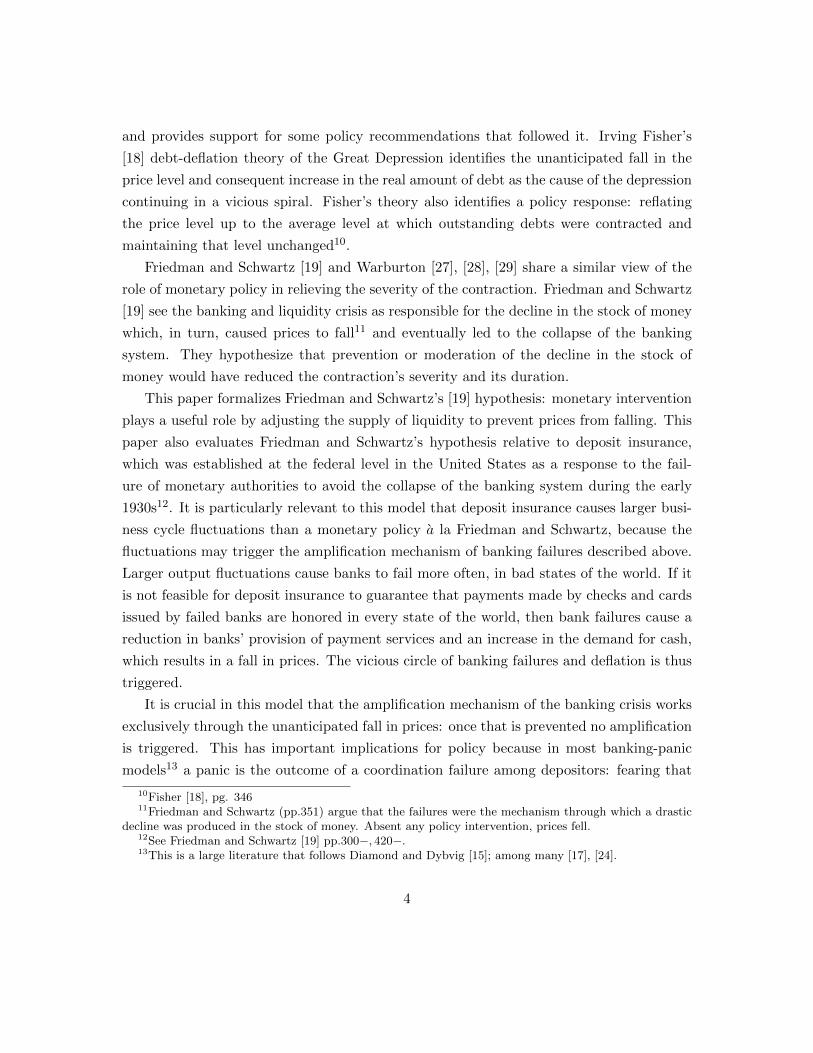
t t+1Nature Banks

θt

δt

Households-Banks

Allocations prices

Figure 2: Timing of players’ moves

payments by banks are due: the interest rate on deposits is thus fixed in nominal terms,

although it is endogenous.

As in the one-period model, banks issue checks, debit and credit cards to households

up to the face value of household’s income at the end of each period, which is the gross

return on deposits and the income from selling cash and credit goods produced with the

labor endowment y.

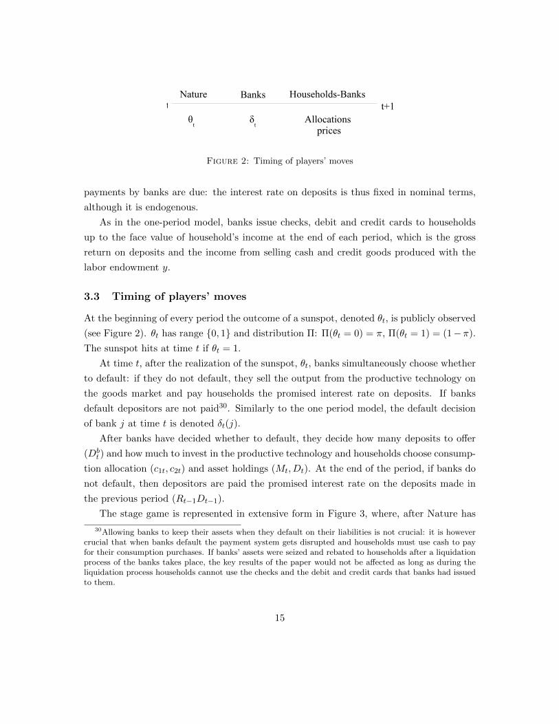
3.3 Timing of players’ moves

At the beginning of every period the outcome of a sunspot, denoted θt, is publicly observed

(see Figure 2). θt has range 0, 1 and distribution Π: Π(θt = 0) = π, Π(θt = 1) = (1−π).

The sunspot hits at time t if θt = 1.

At time t, after the realization of the sunspot, θt, banks simultaneously choose whether

to default: if they do not default, they sell the output from the productive technology on

the goods market and pay households the promised interest rate on deposits. If banks

default depositors are not paid30. Similarly to the one period model, the default decision

of bank j at time t is denoted δt(j).

After banks have decided whether to default, they decide how many deposits to offer

(Dbt ) and how much to invest in the productive technology and households choose consump-

tion allocation (c1t, c2t) and asset holdings (Mt, Dt). At the end of the period, if banks do

not default, then depositors are paid the promised interest rate on the deposits made in

the previous period (Rt−1Dt−1).

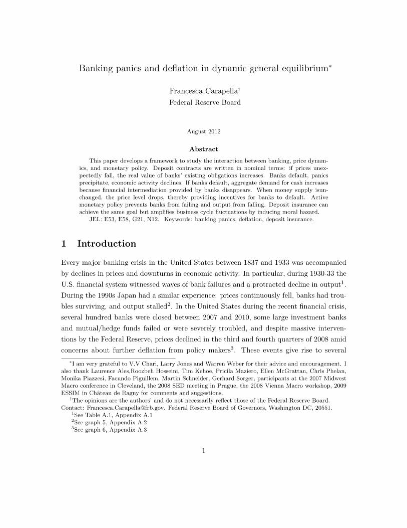
The stage game is represented in extensive form in Figure 3, where, after Nature has

30Allowing banks to keep their assets when they default on their liabilities is not crucial: it is howevercrucial that when banks default the payment system gets disrupted and households must use cash to payfor their consumption purchases. If banks’ assets were seized and rebated to households after a liquidationprocess of the banks takes place, the key results of the paper would not be affected as long as during theliquidation process households cannot use the checks and the debit and credit cards that banks had issuedto them.

15

Nature: θt

0 1

Bank j:

Households:

Dt>0D

t=0 D

t>0

δ jt=1

δ j't=0

δ jt=0

Dt=0

δ j't=1

Bank j':

Dt>0

δ jt=1

δ j't=0

δ jt=0

Dt=0

δ j't=1

Figure 3: Stage Game in extensive form

drawn a realization of θt, bank j chooses whether to default without knowing what other

banks j′ chose: then households choose consumption allocation and asset holdings and

banks choose how much to invest in the productive technology. In particular households

choose whether to deposit a strictly positive amount of assets. For analytical tractability

it is assumed that when a bank defaults then it loses its endowment of labor L forever.

Hence when λt =∫ 10 δt(j)dj = 1, then the banking system shuts down forever: the only

source of output in the economy is households’ endowment and the only means of payment

available to households is cash.

3.4 Players’ strategies

Let ht−1 denote the history of the game at the beginning of time t. ht−1 is anonymous

with respect to households, which are anonymous players in the game, and is a list of past

default decisions by every bank j ∈ [0, 1] (δs(j)j∈[0,1]), sunspot realizations (θt), prices of

consumption goods (ps) and deposits (Rs), aggregate asset holdings by households at the

beginning of every period (As), aggregate consumption of cash good (c1s), of credit good

(c2s), aggregate cash (Ms) and deposits holdings at every bank j (Ds(j)):

ht−1 = (δs(j)j∈[0,1], θs, ps, Rs, As, c1s, c2s, is,Ms, Ds(j)j∈[0,1] | s ≤ t− 1).

Let ht1 = (ht−1, θt, δt(j)j∈[0,1]) denote the history of the game at time t after banks’

default decisions have been made, which includes the history at the beginning of period t,

16

the current realization of the sunspot (θt) and the current default decision of every bank j

(δt(j)j∈[0,1]).

Let the set of possible histories at the beginning of time t be denoted Ht, with H0 = ∅,and the set of possible histories at time t after banks’ default decisions have been made be

denoted Ht1 with H0

1 = θ0, δ0(j)j∈[0,1], so that ht1 is a typical element of Ht1.

A strategy for a household is a mapping σHt : Ht1 → R5

+. After history ht1 is realized,

households’ strategy is σHt (ht1) = (c1t(ht1), c2t(ht1), Dt(ht1),Mt(h

t1), At+1(h

t1)) ∈ R5

+ and a

strategy profile for a representative household is denoted: σH = σHt ∞t=0.

Let µHt : Ht+11 → [0, 1] denote the conditional probability 31 that history ht+1

1 ht1will be realized if ht1 is the realized history at time t. Then a household that starts period

t with assets At and deposits Dt−1, chooses c1t, c2t,Mt, Dt, At+1 to maximize her payoff

at time t after history ht1 has been observed, denoted vt(ht1, At, Dt−1):

vt(ht1, At, Dt−1) = maxU(c1t, c2t) + β

∫ht+1∈Ht+1

µt(ht+11 | ht1)vt+1(h

t+11 , At+1, Dt)dh

t+1 (10)

s.t.

Mt +Dt = At (11)

pt(Ht)c1t ≤ Mt (12)

pt(Ht)(c1t + c2t

)≤ Mt + (1− λt)

(pt(H

t)yt +Rt−1(Ht−1)Dt−1

)(13)

At+1 = Mt − pt(Ht)c1t − pt(Ht)c2t

+ pt(Ht)yt + (1− λt)Rt−1(Ht−1)Dt−1 (14)

As in the one-period-model, constraint (11) is the securities market constraint: the house-

hold splits his assets between cash to carry within the period and deposits at banks.

Constraint (12) is the cash-in-advance constraint on cash goods and constraint (13) is the

credit good constraint. Credit goods can be purchased with unspent cash on cash goods,

and with a fraction, proportional to the measure of non defaulting banks, of the income

from the sales of the endowment and the return on previous period deposits, which are

paid to the households at the end of the period32. Because both are paid at the end of the

31induced by the sunspot distribution and players’ strategies.32As noted in section 2.1 every result is independent of the type of friction introduced between the

securities and the goods’ market. Both a timing friction and physical separation between the workerand the shopper imply that households’ income is not available on the goods’ market and that financialintermediation provided by banks allows households to carry into the period only the cash they need topurchase cash goods.

17

period, they could not be used to pay for consumption purchases if banks were not pro-

viding intermediation by issuing liabilities that can be used as means of payment. Finally,

constraint (14) is the law of motion for assets: assets at the beginning of the next period

are unspent cash, income from the sales of the endowment and a fraction, proportional to

the measure of non defaulting banks, of the return on previous period deposits. As in the

one-period-model, when banks default households lose the return on deposits made in the

previous period but don’t lose their income as a form of wealth: households will still get

paid for the sales of their endowment at the end of the period, because that income stems

from an activity unrelated to banks.

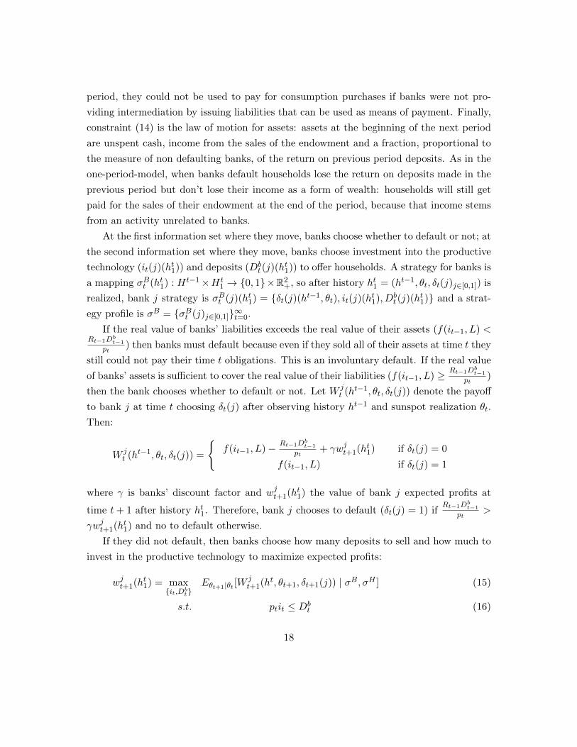
At the first information set where they move, banks choose whether to default or not; at

the second information set where they move, banks choose investment into the productive

technology (it(j)(ht1)) and deposits (Db

t (j)(ht1)) to offer households. A strategy for banks is

a mapping σBt (ht1) : Ht−1×Ht1 → 0, 1×R2

+, so after history ht1 = (ht−1, θt, δt(j)j∈[0,1]) is

realized, bank j strategy is σBt (j)(ht1) = δt(j)(ht−1, θt), it(j)(ht1), Dbt (j)(h

t1) and a strat-

egy profile is σB = σBt (j)j∈[0,1]∞t=0.

If the real value of banks’ liabilities exceeds the real value of their assets (f(it−1, L) <Rt−1Dbt−1

pt) then banks must default because even if they sold all of their assets at time t they

still could not pay their time t obligations. This is an involuntary default. If the real value

of banks’ assets is sufficient to cover the real value of their liabilities (f(it−1, L) ≥ Rt−1Dbt−1

pt)

then the bank chooses whether to default or not. Let W jt (ht−1, θt, δt(j)) denote the payoff

to bank j at time t choosing δt(j) after observing history ht−1 and sunspot realization θt.

Then:

W jt (ht−1, θt, δt(j)) =

f(it−1, L)− Rt−1Dbt−1

pt+ γwjt+1(h

t1) if δt(j) = 0

f(it−1, L) if δt(j) = 1

where γ is banks’ discount factor and wjt+1(ht1) the value of bank j expected profits at

time t+ 1 after history ht1. Therefore, bank j chooses to default (δt(j) = 1) ifRt−1Dbt−1

pt>

γwjt+1(ht1) and no to default otherwise.

If they did not default, then banks choose how many deposits to sell and how much to

invest in the productive technology to maximize expected profits:

wjt+1(ht1) = max

it,DbtEθt+1|θt [W

jt+1(h

t, θt+1, δt+1(j)) | σB, σH ] (15)

s.t. ptit ≤ Dbt (16)

18

Constraint (16) is banks’ budget constraint: investment into productive projects is financed

by the deposits they sold to households33

3.5 Equilibrium characterization

Definition 2 A subgame perfect symmetric equilibrium is:

1. a symmetric strategy profile for households σH = σHt ∞t=0

2. a symmetric strategy profile for banks σB = σBt ∞t=0

3. pricing functions pt(ht1), Rt(h

t1)

34

such that for any t, ht1, households maximize; for any t, ht, banks maximize and prices clear

the markets:

cbt(ht1) + c1t(h

t1) + c2t(h

t1) + it(h

t1) = yt + f(it−1(h

t−11 ), L) (17)

Mt(ht1) +Dt(h

t1) = M t = M (18)

The resource constraint (17) indicates that aggregate consumption by banks and house-

holds, and aggregate investment in the productive technology equal output of cash and

credit good produced by households with labor endowment yt, and the output from banks’

productive technology using t − 1 inputs. The money market clearing condition (18) in-

dicates that aggregate cash and deposit holdings by households equal the stock of money

supply at time t.

Consider equilibria with constant money supply (M t = M) and let U(c1, c2) = log(c1)+

log(c2) and f(it, L) = iαt L1−α. Further assume:

Assumption 4 [αβ2L1−απ]1

1−α < y

Assumption 5 1+[2β(1−π)+βπ[( yαπ)1−α+2(1−π)αβ2L1−α]

[( yαπ)1−α−παβ2L1−α]

]−1 > πα+(Ly )1−α [αβ2L1−α(2−π)]α

[y1−α+2(1−π)αβ2L1−α]α

33A large business cycle literature focuses on the role of credit market frictions on output fluctuations.Such frictions affect firms’ borrowing constraint when undertaking investment projects: see Bernanke andGertler [4], Bernanke, Gertler and Gilchrist [5], and Carlstrom and Fuerst [10]. This is formalized in themodel by assuming that banks’ discount factor γ is small enough so that bankers consume their profits inevery period, as guaranteed by assumption 7. See also appendix C.

34Notice that pricing functions are defined over aggregate histories: Ht = (ht−1, θt,∫ 1

0δt(j)dj). However

aggregate histories are functions of ht1 = (ht−1, θt, (δt(j))j∈[0,1]), since they are defined over the aggregatedefault decisions by banks rather than on each bank j default decision. Therefore ultimately pricingfunctions pt and Rt are functions of ht1.

19

Assumption 6 απ < 1

Assumption 7 Either γ < β2 or γ > β2(2− π)

Assumption 8 α(1−γπ)πγ(1−α) < 1

Under the above assumptions there exists a symmetric equilibrium in this economy such

that no default occurs until the first date t at which the sunspot hits (θt = 1): then banks

fail, households don’t deposit in any bank, prices decline and aggregate output falls. There

is no banking system after that35.

Proposition 2 Let t denote the first date at which the sunspot hits (θt = 1). If Assump-

tions 4-6 are satisfied then there exists a symmetric equilibrium such that:

• λs =∫ 10 δs(j)dj = 0, Ds(j) = Dnd > 0 ∀j ∈ [0, 1], ps = pnd, ∀s < t

• λs =∫ 10 δs(j)dj = 1, Ds(j) = 0 ∀j ∈ [0, 1], ps = pd, ∀s ≥ t

• pd < pnd

• Ys =

y ∀s ≥ t+ 1

y + f(i(hs1), L) ∀s ≤ t

Proof See Appendix B.

Proposition 2 generalizes proposition 1 to a dynamic environment where banks make strate-

gic default decisions, and where deposits and banks’ production are explicitly linked. Banks

default when the actual price is too low relative to the price their nominal liabilities are

indexed to, and when banks default the payment services they would normally provide are

no longer viable. The only means of payment available in the economy is now cash, causing

the set of goods that are purchased using cash to expand. To the extent that the ratio of

goods purchased by cash to the amount of cash brought within the period is larger than

in no default, then prices fall.

Also, because the deposit decision is dynamic and influenced by the probability that

the bank will not be insolvent, this version of the model highlights the impact of a banking

35This is done for analytical tractability. Letting banks come back in business after failing or letting newbanks enter the market after banking failures have occurred, would require evaluating banks’ continuationpayoffs at allocations that are not time invariant.

20

panic on investment and ultimately on aggregate output. When banks fail, households are

not paid and do not deposit their assets at any bank, so a banking panic occurs36. No

investment into the productive technology f takes place, since deposits are the only source

of funds for banks to purchase production inputs, so aggregate output falls.

3.6 Monetary policy and the Friedman and Schwartz hypothesis

This section analyzes the relationship between banking and monetary policy.

In the environment described in sections 3.1-3.5 consider a monetary authority endowed

with a printing money technology, who can commit to future policies and moves after banks

decided whether to default or not, so the relevant history of the game at its information

set is ht1.

For analytical tractability the focus is on a one time policy experiment in period t. Let

the economy start from the equilibrium described in proposition 2 so that banks’ existing

deposits Dt−1 = Dnd. Let the monetary authority adopt the following active policy: if a

positive measure of banks defaults at time t then it injects cash on the securities market

to households in the amount Tt(ht1), otherwise it leaves M unchanged. The amount of the

money injection Tt(ht1) is just enough to keep current prices constant with respect to the

previous period, and is a function of the measure of banks that defaulted at the beginning

of the period. If a measure one of banks defaults (λt = 1) then Tt(ht1) = pndy − M

so that the new stock of money supply is M′(ht1) = M + Tt(h

t1) = pndy. Then time t

prices in equilibrium are pt = pnd because when the banking system collapses (λt = 1)

any consumption good that households buy must be paid in cash (their cash in advance

constraint is pt(c1t + c2t) = M′(ht1)), and they buy a total of y goods. If a smaller measure

of banks defaults then the cash transfer necessary to keep prices at no-default level (pnd)

will be smaller. Proposition 3 shows that if the monetary authority follows this active

policy, then when the sunspot hits it is no longer optimal for banks to default.

Proposition 3 Under assumptions 4-6 the unique pure strategy equilibrium with an active

monetary policy is no default and no panics at time 0 and no decline in economic activity.

Proof See appendix B.

36Because the focus is not what drives depositors to run on banks, banking panics in this model areidentified with households not being paid for the claims they had on banks.

21

This result shows that the Friedman-Schwartz hypothesis is correct in this environment:

an active monetary policy would have been effective in the early 1930s at preventing prices

from falling and banking panics from occurring. By avoiding massive bank failures, an

active monetary policy would have prevented the collapse of the stock of money and the

banking system, thus resulting in a milder cycle37.

Monetary policy in this environment is very powerful: banking crises arise solely from

a fall in prices because banks’ liabilities are fixed in nominal terms. Because prices are

determined in the market for cash goods, by affecting the stock of money that is brought

to the goods’ market, the monetary authority can influence prices. The commitment by

the monetary authority to keep prices constant is enough to give banks incentives not to

default, therefore no failures and no deflation occur in equilibrium. Depositors do not

panic and economic activity does not decline. Commitment to price stability is sufficient

to discipline off equilibrium payoffs and sustain no default in equilibrium, with no actual

money injections taking place.

3.7 Deposit Insurance

This section studies the effectiveness of deposit insurance in the environment described

in sections 3.1-3.5 and evaluates it relative to the monetary policy described in section

3.6. If coupled with strict regulatory arrangements deposit insurance can prevent banking

panics. Absent strict regulatory arrangements, deposit insurance can prevent banking

panics but also induces larger output fluctuations than monetary policy interventions,

because it induces moral hazard on the part of banks.

In order to study moral hazard incentives for banks, let the set of productive tech-

nologies that banks can invest in include both the safe technology introduce in section 3.5,

f(it, L) = iαt L1−α, and a risky technology: f(it, L) = riαt L

1−α where r is a random variable

defined over a probability space (Ω,F , P ), so that r : Ω→ X = r, r with r > 138. Define

A = ω ∈ Ω : r(ω) = r as the event where the risky technology has high return, r. The

distribution of r is P (A) = q and P (AC

) = 1 − q. r is an aggregate shock and it is such

that qr + (1− q)r < 1 so that f is a mean reducing spread of f . Also, r is independent of

the sunspot and i.i.d over time.

For analytical tractability the focus is on a one-time policy experiment in period t.

37See Friedman and Schwartz [19], in The Great Contraction- Origin of Bank Failures.38If r ≤ 1 then there are no interesting trade offs since banks would always choose f because it dominates

f in every state of the world.

22

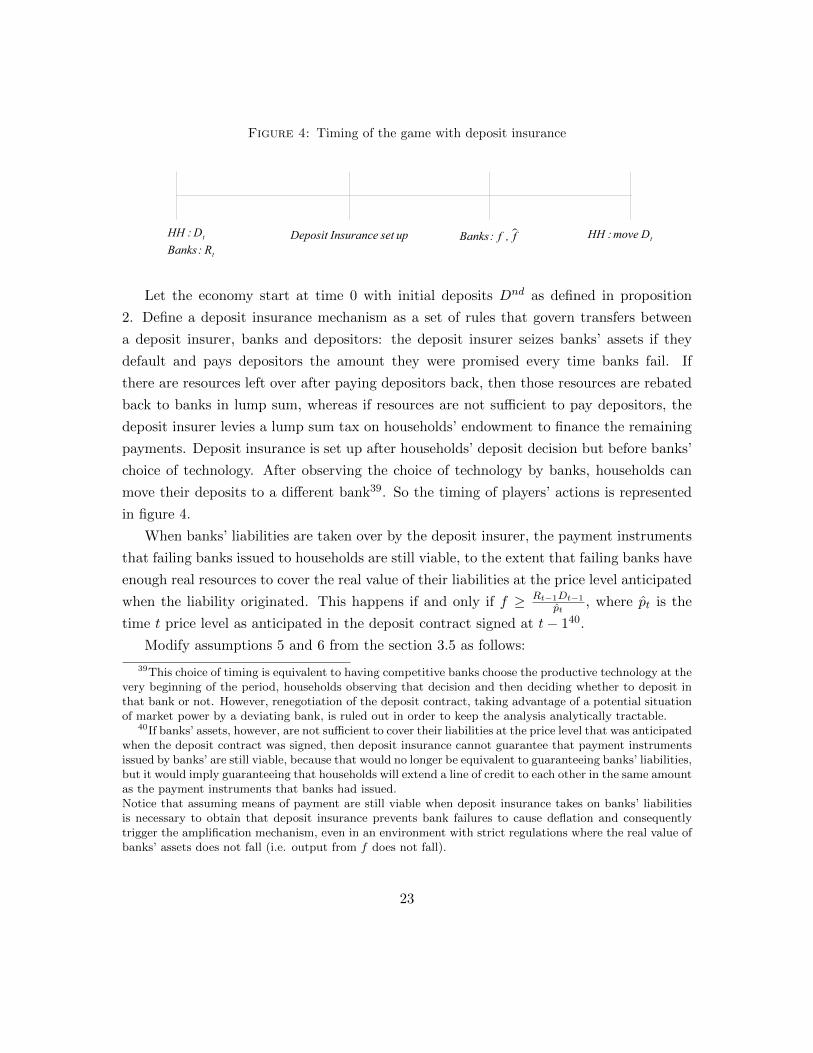
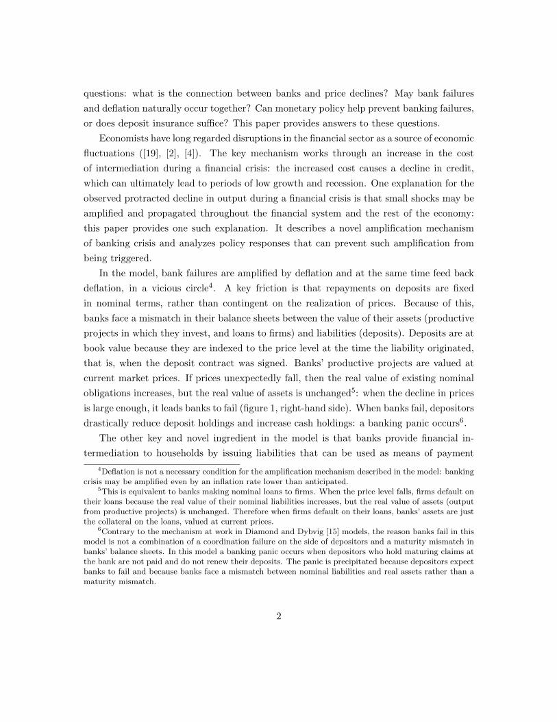
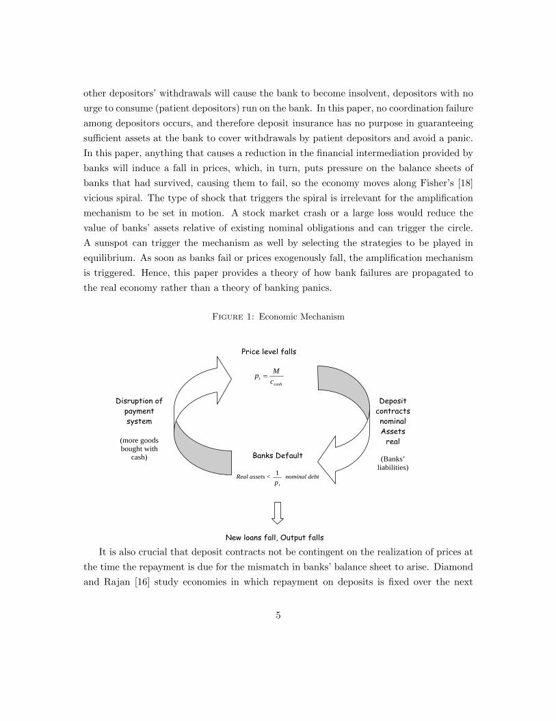
Figure 4: Timing of the game with deposit insurance

Banks: f , !fDeposit Insurance set upHH :Dt

Banks: Rt

HH :move Dt

Let the economy start at time 0 with initial deposits Dnd as defined in proposition

2. Define a deposit insurance mechanism as a set of rules that govern transfers between

a deposit insurer, banks and depositors: the deposit insurer seizes banks’ assets if they

default and pays depositors the amount they were promised every time banks fail. If

there are resources left over after paying depositors back, then those resources are rebated

back to banks in lump sum, whereas if resources are not sufficient to pay depositors, the

deposit insurer levies a lump sum tax on households’ endowment to finance the remaining

payments. Deposit insurance is set up after households’ deposit decision but before banks’

choice of technology. After observing the choice of technology by banks, households can

move their deposits to a different bank39. So the timing of players’ actions is represented

in figure 4.

When banks’ liabilities are taken over by the deposit insurer, the payment instruments

that failing banks issued to households are still viable, to the extent that failing banks have

enough real resources to cover the real value of their liabilities at the price level anticipated

when the liability originated. This happens if and only if f ≥ Rt−1Dt−1

pt, where pt is the

time t price level as anticipated in the deposit contract signed at t− 140.

Modify assumptions 5 and 6 from the section 3.5 as follows:

39This choice of timing is equivalent to having competitive banks choose the productive technology at thevery beginning of the period, households observing that decision and then deciding whether to deposit inthat bank or not. However, renegotiation of the deposit contract, taking advantage of a potential situationof market power by a deviating bank, is ruled out in order to keep the analysis analytically tractable.

40If banks’ assets, however, are not sufficient to cover their liabilities at the price level that was anticipatedwhen the deposit contract was signed, then deposit insurance cannot guarantee that payment instrumentsissued by banks’ are still viable, because that would no longer be equivalent to guaranteeing banks’ liabilities,but it would imply guaranteeing that households will extend a line of credit to each other in the same amountas the payment instruments that banks had issued.Notice that assuming means of payment are still viable when deposit insurance takes on banks’ liabilitiesis necessary to obtain that deposit insurance prevents bank failures to cause deflation and consequentlytrigger the amplification mechanism, even in an environment with strict regulations where the real value ofbanks’ assets does not fall (i.e. output from f does not fall).

23

Assumption 9 1+[2β(1−π)+βπ[( yαπr

)1−α+2(1−π)αβ2L1−α]

[( yαπr

)1−α−παβ2L1−α]]−1 > πr

α +r(Ly )1−α [αβ2L1−α(2−π)]α[y1−α+2(1−π)αβ2L1−α]α

Assumption 10 αE(r)qπ < 1

Let z = γ(1−α)1−γπ −

απ and further assume:

Assumption 11 q > q = 1+zr+z

The following proposition draws results on the effectiveness of deposit insurance at prevent-

ing banking panics, and on its effects on output and prices. Deposit insurance is analyzed

in two regulatory environments: one with strict regulations, where the insurer can force

banks to invest only in the safe technology, and one without strict regulations, where banks

cannot be forced to invest in a specific technology.

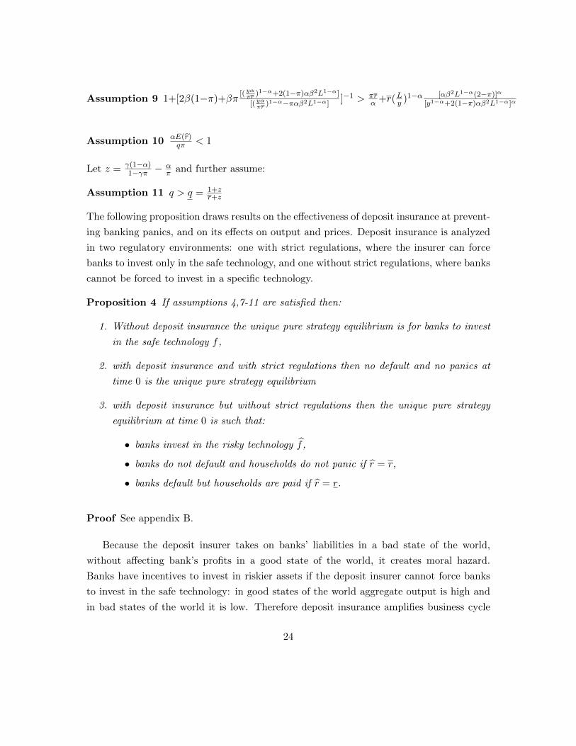
Proposition 4 If assumptions 4,7-11 are satisfied then:

1. Without deposit insurance the unique pure strategy equilibrium is for banks to invest

in the safe technology f ,

2. with deposit insurance and with strict regulations then no default and no panics at

time 0 is the unique pure strategy equilibrium

3. with deposit insurance but without strict regulations then the unique pure strategy

equilibrium at time 0 is such that:

• banks invest in the risky technology f ,

• banks do not default and households do not panic if r = r,

• banks default but households are paid if r = r.

Proof See appendix B.

Because the deposit insurer takes on banks’ liabilities in a bad state of the world,

without affecting bank’s profits in a good state of the world, it creates moral hazard.

Banks have incentives to invest in riskier assets if the deposit insurer cannot force banks

to invest in the safe technology: in good states of the world aggregate output is high and

in bad states of the world it is low. Therefore deposit insurance amplifies business cycle

24

fluctuations. If the deposit insurer could force banks to invest only in the safe technology,

then it would achieve the same outcome as a monetary policy aimed at keeping prices

constant (proposition 4.2). Also, proposition 4.1 guarantees that none of the results in

propositions 2 and 3 change when banks are allowed to choose between f and f : without

deposit insurance banks choose to invest in the safe technology f : propositions 2 and 3 go

through.

The results in proposition 4 contribute to the literature that studies the tradeoffs asso-

ciated with deposit insurance. Previous work has mostly focused on designing appropriate

incentive schemes to control the moral hazard induced by insurance; some research has

pointed out alternative policies to deposit insurance that do not induce moral hazard,

under certain conditions.

This paper takes a different approach: it points out an additional channel through

which moral hazard can be very costly. Deposit insurance may trigger the amplification

mechanism of banking failures through deflation to the extent that it does not always41

guarantee that payments by checks and cards issued by failed banks will be honored. If

such payments cannot be honored, then even in an environment with strict regulations

deposit insurance cannot achieve the same equilibrium outcome as the monetary policy of

proposition 3, because any sunspot realization may trigger the vicious circle. In an environ-

ment without strict regulations, any low realization of banks’ risky technology triggers the

circle, because in this state of the world deposit insurance cannot guarantee that payment

instruments issued by failing banks are still viable.

4 Conclusion

Starting with Fisher’s [18] debt-deflation theory of the Great Depression and subsequently

Friedman and Schwartz’s [19] seminal work on the monetary history of the United States,

monetary forces were considered a potent instrument for promoting economic stability, by

preventing or moderating large price declines.

Later work has focused on the role of banks in the provision of liquidity and their

fragility due to the maturity transformation banks provide: this literature has helped

41Suppose for instance that the resources deposit insurance can gather by taxing households are notsufficient to cover payments to depositors: then banks’ liabilities cannot be guaranteed, and so checks andcards payments. One such example is when households’ production is a random variable correlated with r,such that if at time t rt = r then yt is low, so low that the insurer cannot feasibly raise enough resourcesto pay depositors.

25

understanding the economic rationale for many institutional arrangements that took place

after the Great Depression and even challenged them ([15], [11], [13], [17], [21], [24]).

Recent work placed banks’ fragility along another perspective drawing from Fisher’s

[18] idea: the existence of frictions in contracting prevents state contingent repayment on

deposits. Any shock that was not anticipated at the time the deposit contract was signed

may impair banks’ solvency. Therefore monetary intervention can help offset monetary

and real shocks by keeping the price level stable, thus limiting the future real repayment

obligations of banks ([16]).

This paper further investigates such a mechanism showing that when repayment on

deposit contracts is fixed in nominal terms over the next instant, and when banks provide

financial intermediation through payment services, banking difficulties may be endoge-

nously amplified, in a vicious circle. When banks’ payment services decrease, households’

demand for cash increases, which induces prices to fall. When prices fall, the real burden

of existing nominal obligations increases relative to assets, leading banks to be illiquid and

fail.

In this environment monetary intervention is very powerful: adjusting the supply of

liquidity to aggregate conditions, it prevents the amplification mechanism from being trig-

gered, ensuring that the banking system is not destabilized. Because price declines are

the cause of bank failures, deposit insurance cannot tackle the root of the problem, to

the extent that it doesn’t affect prices to counteract changes in aggregate liquidity condi-

tions. Nonetheless, by insuring banks’ liabilities it still prevents panics, in the sense that

depositors are paid their claims on banks. By insuring banks’ liabilities, however, deposit

insurance induces moral hazard, thus resulting in larger business cycle fluctuation than

monetary policy would.

This suggests an important role for monetary policy in stabilizing the banking system.

It also suggests that further investigation of the frictions that lead to difficulties in con-

tracting resulting in fixed repayments should be fostered, as well as mechanisms that, given

those frictions, may be welfare improving relative to fixed repayment arrangements42.

42The trade off between real versus nominal contracts is analyzed by Diamond and Rajan [16] but theystill assume contracts with a fixed repayment over the next instant.

26

A Appendix

A.1 United States between 1837 and 1933

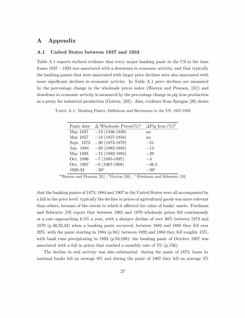
Table A.1 reports stylized evidence that every major banking panic in the US in the time

frame 1837−1933 was associated with a downturn in economic activity, and that typically

the banking panics that were associated with larger price declines were also associated with

more significant declines in economic activity. In Table A.1 price declines are measured

by the percentage change in the wholesale prices index (Warren and Pearson, [31]) and

slowdown in economic activity is measured by the percentage change in pig iron production

as a proxy for industrial production (Gorton, [20]). Also, evidence from Sprague [26] shows

Table A.1: Banking Panics, Deflations and Recessions in the US: 1837-1933

Panic date ∆ Wholesale Prices(%)a ∆Pig Iron (%)b

May 1837 −13 (1836-1838) naMay 1857 −13 (1857-1858) naSept. 1873 −30 (1873-1879) −51Jun. 1884 −20 (1882-1885) −14May 1893 −15 (1892-1894) −29Oct. 1896 −7 (1895-1897) −4Oct. 1907 −6 (1907-1908) −46.51929-33 −30c −50c

aWarren and Pearson [31] , bGorton [20] , c Friedman and Schwartz [19]

that the banking panics of 1873, 1884 and 1907 in the United States were all accompanied by

a fall in the price level: typically the decline in prices of agricultural goods was more relevant

than others, because of the extent to which it affected the value of banks’ assets. Friedman

and Schwartz [19] report that between 1865 and 1879 wholesale prices fell continuously

at a rate approaching 6.5% a year, with a sharper decline of over 30% between 1873 and

1879 (p.30,32,42) when a banking panic occurred; between 1882 and 1885 they fell over

20%, with the panic starting in 1884 (p.94); between 1892 and 1894 they fell roughly 15%,

with bank runs precipitating in 1893 (p.94,108); the banking panic of October 1907 was

associated with a fall in prices that reached a monthly rate of 5% (p.156).

The decline in real activity was also substantial: during the panic of 1873, loans by

national banks fell on average 9% and during the panic of 1907 they fell on average 2%

27

(Sprague, 1910, p.305-310).

For the banking panics that occurred during the Great Depression Friedman and

Schwartz [19] offer a detailed description of the extent of the fall in prices and economic

activity: prices fell 36% and industrial production roughly 50% over the course of 1929-

1933 (p.303). During the same time frame banking panics were quite frequent (Friedman

and Schwartz, [19], p.308-328). Also Fisher [18], Calomiris [6], Calomiris and Mason [8],

and Warren and Pearson [31] argue that the fall in the price level significantly reduced the

value of firms and banks’ assets relative to the value of their liabilities, forcing them to fail.

Furthermore, Wicker [33] offers evidence that currency usage replaced checks during

the banking failures of the Great Depression43, and, for the same time period, Richardson

[25] documents the critical role played by payment system’s disruptions in the propagation

of banking panics44 especially through the failure of correspondent banks45.

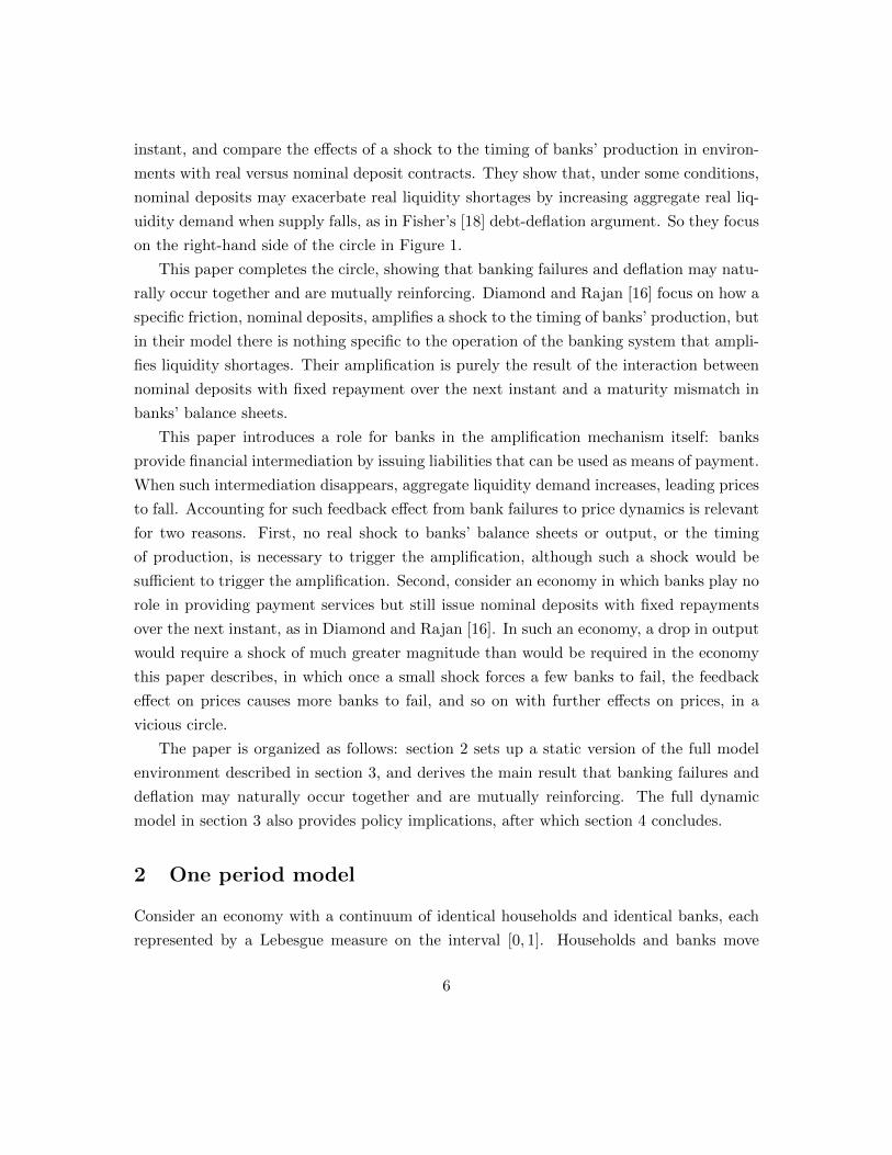
A.2 Japan during the 1990s

In Japan during the 1990s, often referred to as the Lost Decade, prices fell considerably

(1.5% every year since mid 1990s until 2002) and real activity grew on average only 1% every

year during the period 1991-200246: the existence of a deposit insurance agency prevented

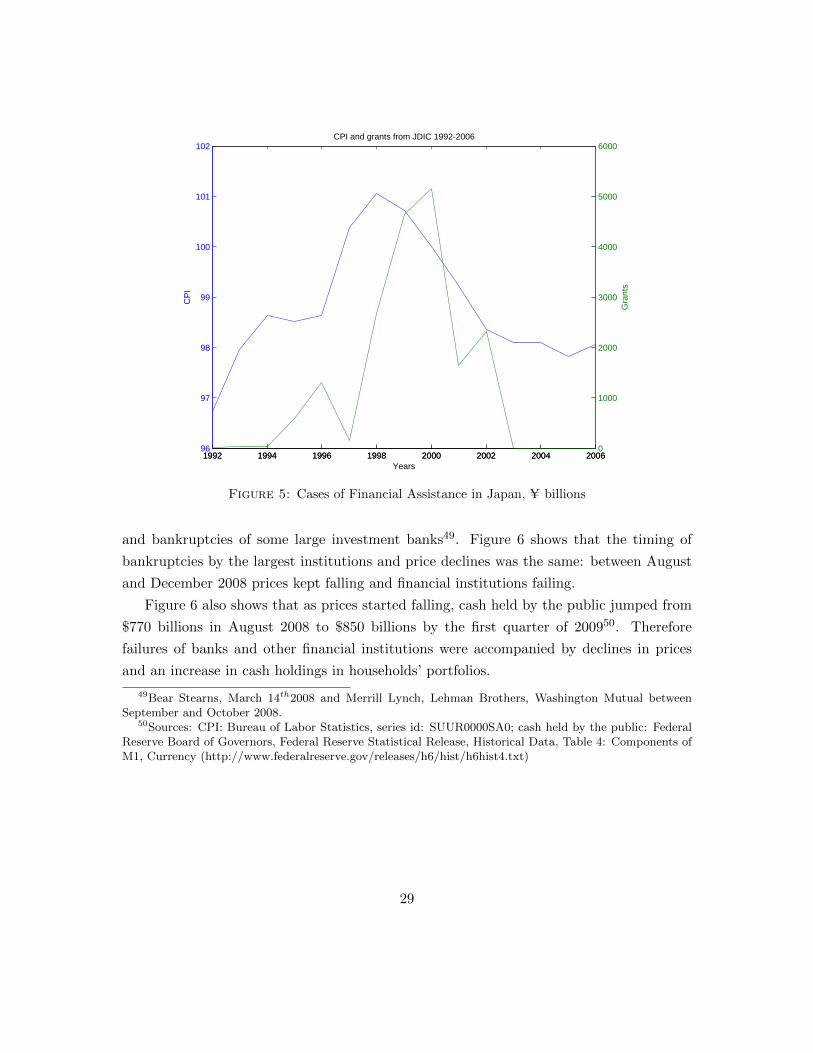
bank runs but banking difficulties and banking failures were widespread. Figure 5 shows

that at the same time as prices started falling, between 1998 and 2003, financial assistance

granted by the Japan Deposit Insurance Corporation to banks increased dramatically going

from nearly zero in 1997 to 5 trillions U in 2000, then remaining substantially high around

2 trillions U until 2002 while prices kept falling until 200347.

A.3 US: 2007-2010

The United States between 2007 and 2010 experienced very low inflation which turned into

deflation in the second half of 2008, accompanied by several hundreds of banking failures48

43[33], pg. 4544See pg. 64445Correspondent banks were banks that cleared checks for other banks (respondents).46 Baba et al., [1]47Sources: CPI: International Financial Statistics, Consumer Prices; Grants by JDIC: Deposit Insurance

Corporation of Japan, DICJ’s Activities, Financial Assistance.48See Failed Financial Institutions, FDIC public website

28

1992 1994 1996 1998 2000 2002 2004 200696

97

98

99

100

101

102

CP

I

Years

CPI and grants from JDIC 1992-2006

1992 1994 1996 1998 2000 2002 2004 20060

1000

2000

3000

4000

5000

6000

Gra

nts

Figure 5: Cases of Financial Assistance in Japan, U billions

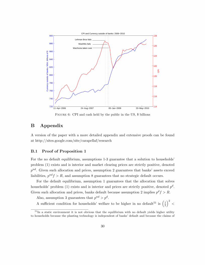
and bankruptcies of some large investment banks49. Figure 6 shows that the timing of

bankruptcies by the largest institutions and price declines was the same: between August

and December 2008 prices kept falling and financial institutions failing.

Figure 6 also shows that as prices started falling, cash held by the public jumped from

$770 billions in August 2008 to $850 billions by the first quarter of 200950. Therefore

failures of banks and other financial institutions were accompanied by declines in prices

and an increase in cash holdings in households’ portfolios.

49Bear Stearns, March 14th2008 and Merrill Lynch, Lehman Brothers, Washington Mutual betweenSeptember and October 2008.

50Sources: CPI: Bureau of Labor Statistics, series id: SUUR0000SA0; cash held by the public: FederalReserve Board of Governors, Federal Reserve Statistical Release, Historical Data, Table 4: Components ofM1, Currency (http://www.federalreserve.gov/releases/h6/hist/h6hist4.txt)

29

11−Apr−2006 24−Aug−2007 05−Jan−2009 20−May−2010720

740

760

780

800

820

840

860

880

900CPI and Currency outside of banks: 2006−2010

Cur

renc

y ou

tsid

e of

ban

ks, N

SA

, bill

ions

of $

114

116

118

120

122

124

126

128

CP

I

WashMu fails

Lehman Bros fails

Wachovia taken over

Figure 6: CPI and cash held by the public in the US, $ billions

B Appendix

A version of the paper with a more detailed appendix and extensive proofs can be found

at http://sites.google.com/site/carapellaf/research

B.1 Proof of Proposition 1

For the no default equilibrium, assumptions 1-3 guarantee that a solution to households’

problem (1) exists and is interior and market clearing prices are strictly positive, denoted

pnd. Given such allocation and prices, assumption 2 guarantees that banks’ assets exceed

liabilities, pndf > R, and assumption 8 guarantees that no strategic default occurs.

For the default equilibrium, assumption 1 guarantees that the allocation that solves

households’ problem (1) exists and is interior and prices are strictly positive, denoted pd.

Given such allocation and prices, banks default because assumption 2 implies pdf > R.

Also, assumption 3 guarantees that pnd > pd.

A sufficient condition for households’ welfare to be higher in no default51 is(12

)2<

51In a static environment it is not obvious that the equilibrium with no default yields higher utilityto households because the planting technology is independent of banks’ default and because the claims of

30

(rA

[r(1+r)A−R(2r−1)]√r(1 + r)

(3r−22r−1

) 12)2

which is satisfied by assumption 2.

B.2 Proof of Proposition 2

The equilibrium is constructed by defining strategies for banks and households as follows:

banks default if the sunspot hits and do not default otherwise. Households do not deposit

in bank j if bank j defaults and deposit Dnd to solve households’ problem (10) otherwise.

Let xst = (cs1t, cs2t,M

st , D

st , A

st+1) denote the allocation that solves the households’ prob-

lem with the constructed strategies, where s = d, nd according to whether banks default

or not.

When the sunspot hits, the solution to the households’ problem is such that cd1 = cd2 =M2pd

since the relevant cash in advance constraint is (13). Then the resource constraint:

f(Dnd

pnd, L) + M

pd= y + f(D

nd

pnd, L), implies pd = M

y .

Before the sunspot hits, assumption 4 guarantees that a solution to the households’

problem exists and is interior. Given allocation xnd and prices pnd, assumption 6 guarantees

that banks’ net assets are strictly positive, f(ind, L) − RndDnd

pnd= (ind)αL1−α(1 − α

π ) > 0,

and assumption 8 guarantees that the real value of paying depositors back is smaller than

the present discounted value of future profits: RndDnd

pnd< γwj,nd. Therefore at prices pnd

banks are solvent and no strategic default occurs.

At prices pd a bank j defaults if and only if f(ind, L)−RndDnd

pd= (ind)αL1−α(1− α

πpnd

pd) <

0 that is to say if and only if pd

pnd< α

π , which is satisfied by assumption 5.

Assumptions 4-5 then imply that pnd > pd.

coconut that households have on banks are exogenous. In the default equilibrium households’ utility lossis caused by financial disintermediation (no payment instruments alternative to cash) and by the loss ofwealth (R units of coconut). However there is a utility gain caused by equalizing the marginal rate ofsubstitution between cash and credit goods with the marginal rate of transformation because the relevantcash-in-advance constraint binds on both goods. Therefore, for the no default equilibrium to yield higherutility to households, it must be the case that the loss is large enough.In a dynamic environment, because households’ claims on banks are linked to the deposit decision, thenthe allocation of consumption and asset holdings that solves the households’ problem in default, say xd, isstill in households’ constraint set in no default. Therefore if a solution to the households’ problem in nodefault, say xnd, is different from xd, it must be the case that households’ utility is higher in no default.

31

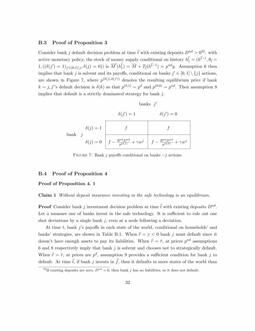
B.3 Proof of Proposition 3

Consider bank j default decision problem at time t with existing deposits Dnd > 052. with

active monetary policy, the stock of money supply conditional on history ht1 = (ht−1, θt =

1, ((δ(j′) = 1)j′∈[0,1]\j , δ(j) = 0)) is M′(ht1) = M + Tt(h

t−1) = pndy. Assumption 6 then

implies that bank j is solvent and its payoffs, conditional on banks j′ ∈ [0, 1] \ j actions,

are shown in Figure 7, where p(δ(j),δ(j′)) denotes the resulting equilibrium price if bank

k = j, j′’s default decision is δ(k) so that p(0,1) = pd and p(0,0) = pnd. Then assumption 8

implies that default is a strictly dominated strategy for bank j.

bank j

banks j′

δ(j′) = 1 δ(j′) = 0

δ(j) = 1 f f

δ(j) = 0 f − RndDnd

p(0,1)+ γwj f − RndDnd

p(0,0)+ γwj

Figure 7: Bank j payoffs conditional on banks −j actions.

B.4 Proof of Proposition 4

Proof of Proposition 4. 1

Claim 1 Without deposit insurance investing in the safe technology is an equilibrium.

Proof Consider bank j investment decision problem at time t with existing deposits Dnd.

Let a measure one of banks invest in the safe technology. It is sufficient to rule out one

shot deviations by a single bank j, even at a node following a deviation.

At time t, bank j’s payoffs in each state of the world, conditional on households’ and

banks’ strategies, are shown in Table B.1. When r = r < 0 bank j must default since it

doesn’t have enough assets to pay its liabilities. When r = r, at prices pnd assumptions

6 and 8 respectively imply that bank j is solvent and chooses not to strategically default.

When r = r, at prices are pd, assumption 9 provides a sufficient condition for bank j to

default. At time t, if bank j invests in f , then it defaults in more states of the world than

52If existing deposits are zero, Dnd = 0, then bank j has no liabilities, so it does not default.

32

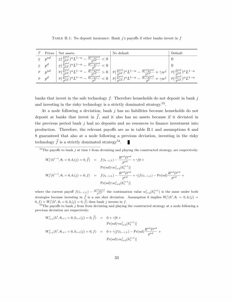
Table B.1: No deposit insurance: Bank j’s payoffs if other banks invest in f

r Prices Net assets No default Default

r pnd r(Dnd

pnd)αL1−α − RndDnd

pnd< 0 0

r pd r(Dnd

pnd)αL1−α − RndDnd

pd< 0 0

r pnd r(Dnd

pnd)αL1−α − RndDnd

pnd> 0 r(D

nd

pnd)αL1−α − RndDnd

pnd+ γwj r(D

nd

pnd)αL1−α

r pd r(Dnd

pnd)αL1−α − RndDnd

pd< 0 r(D

nd

pnd)αL1−α − RndDnd

pd+ γwj r(D

nd

pnd)αL1−α

banks that invest in the safe technology f . Therefore households do not deposit in bank j

and investing in the risky technology is a strictly dominated strategy.53.

At a node following a deviation, bank j has no liabilities because households do not

deposit at banks that invest in f , and it also has no assets because if it deviated in

the previous period bank j had no deposits and no resources to finance investment into

production. Therefore, the relevant payoffs are as in table B.1 and assumptions 6 and

8 guaranteed that also at a node following a previous deviation, investing in the risky

technology f is a strictly dominated strategy54.

53The payoffs to bank j at time t from deviating and playing the constructed strategy, are respectively:

W jt (ht−1, θt = 0, δt(j) = 0, f) = f(it−1,L) − RndDnd

pnd+ γ[0 +

Pr(nd)γwjt+2(ht+11 )]

W jt (ht−1, θt = 0, δt(j) = 0, f) = f(it−1,L) − RndDnd

pnd+ γ[f(it−1,L) − Pr(nd)

RndDnd

pnd+

Pr(nd)γwjt+2(ht+11 )]

where the current payoff f(it−1,L) − RndDnd

pnd the continuation value wjt+2(ht+11 ) is the same under both

strategies because investing in f is a one shot deviation. Assumption 6 implies W jt (ht, θt = 0, δt(j) =

0, f) > W jt (ht, θt = 0, δt(j) = 0, f) then bank j invests in f .

54The payoffs to bank j from from deviating and playing the constructed strategy at a node following aprevious deviation are respectively:

W jt+1(ht, θt+1 = 0, δt+1(j) = 0, f) = 0 + γ[0 +

Pr(nd)γwjt+2(ht+11 )]

W jt+1(ht, θt+1 = 0, δt+1(j) = 0, f) = 0 + γ[f(it−1,L) − Pr(nd)

RndDnd

pnd+

Pr(nd)γwjt+2(ht+11 )]

33

Claim 2 Without deposit insurance investing in the risky technology is not an equilibrium.

Proof Suppose there exists an equilibrium where banks invest in the risky technology. It is

easy to construct a profitable deviation for bank j as follows: invest in the safe technology

f today, offer households the same deposit contract as other banks investing in f offer,

and follow the same strategy played by other banks from tomorrow on. The interest rate

on deposit contracts offered by banks investing in f is Rs = ps+1

ps

E(r)qπ α(Dsps )α−1L1−α and

assumption 10 guarantees that it is always feasible for bank j to offer the same contract55.

Then the expected continuation payoff to bank j is the same as the continuation payoff

to every bank investing in f . The current payoff from investing in f , however, is strictly

larger because f is a mean reducing spread of f . Therefore investing in f is a profitable

deviation for bank j.

Proof of Proposition 4. 2

Proof If a measure one of banks does not default, Proposition 2 implies that the unique

best response for an individual bank is not to default as well.

If the sunspot hits at time t and a measure one of banks defaults then banks’ assets

are seized by the deposit insurer, and their real value is f(ind, L) = r(ind)αL1−α. The

real value of banks’ liabilities to the insurer is RndDnd

ptwhere pt is the price level at time

t. Since real resources exceed the real value of liabilities at the price level anticipated in

the deposit contract, then with deposit insurance bank-issued payment instruments are

still viable, and the solution to the households’ problem is the same as in no default:

(cnd1 , cnd2 , Dnd,Mnd, ind) and the resulting equilibrium price is pt = pnd. Assumptions 6,

8 then guarantee that banks’ net assets are strictly positive and that the payoff from

strategic default is smaller than the payoff from being in business. Therefore the unique

best response for an individual bank is not to default.

Proof of Proposition 4. 3

Assumption 6 implies W jt+1(ht, θt+1 = 0, δt+1(j) = 0, f) > W j

t+1(ht, θt+1 = 0, δt+1(j) = 0, f).55Its assets net of liabilities would be:

iαsL1−α − ps+1

ps

E(r)

qπα(Dsps

)α−1L1−αDsps

= (Dsps

)αL1−α − ps+1

ps

E(r)

qπα(Dsps

)α−1L1−αDsps

= (1 − E(r)α

qπ)(Dsps

)αL1−α > 0

34

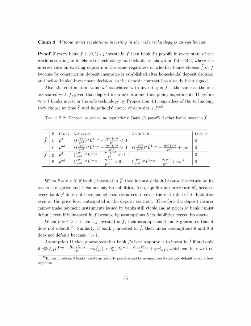
Claim 3 Without strict regulations investing in the risky technology is an equilibrium.

Proof If every bank j′ ∈ [0, 1] \ j invests in f then bank j’s payoffs in every state of the

world according to its choice of technology and default are shown in Table B.2, where the

interest rate on existing deposits is the same regardless of whether banks choose f or f

because by construction deposit insurance is established after households’ deposit decision

and before banks’ investment decision, so the deposit contract has already been signed.

Also, the continuation value wj associated with investing in f is the same as the one

associated with f , given that deposit insurance is a one time policy experiment. Therefore

∀t > t banks invest in the safe technology by Proposition 4.1, regardless of the technology

they choose at time t, and households’ choice of deposits is Dnd.

Table B.2: Deposit insurance, no regulations: Bank j’s payoffs if other banks invest in f

r Prices Net assets No default Default

f r pd r(Dnd

pnd)αL1−α − RndDnd

pd< 0 0

r pnd r(Dnd

pnd)αL1−α − RndDnd

pnd> 0 r(D

nd

pnd)αL1−α − RndDnd

pnd+ γwj 0

f r pd (Dnd

pnd)αL1−α − RndDnd

pd< 0 0

r pnd (Dnd

pnd)αL1−α − RDnd

pnd> 0 (D

nd

pnd)αL1−α − RDnd

pnd+ γwj 0

When r = r < 0, if bank j invested in f , then it must default because the return on its

assets is negative and it cannot pay its liabilities. Also, equilibrium prices are pd, because

every bank j′ does not have enough real resources to cover the real value of its liabilities

even at the price level anticipated in the deposit contract. Therefore the deposit insurer

cannot make payment instruments issued by banks still viable and at prices pd bank j must

default even if it invested in f because by assumptions 5 its liabilities exceed its assets.

When r = r > 1, if bank j invested in f , then assumptions 6 and 8 guarantee that it

does not default56. Similarly, if bank j invested in f , then under assumptions 6 and 8 it

does not default because r > 1.

Assumption 11 then guarantees that bank j’s best response is to invest in f if and only

if q[riαt−1L1−α− Rt−1Dt−1

pt+γwjt+1] > [iαt−1L

1−α− Rt−1Dt−1

pt+γwjt+1], which can be rewritten

56By assumptions 6 banks’ assets are strictly positive and by assumption 8 strategic default is not a bestresponse.

35

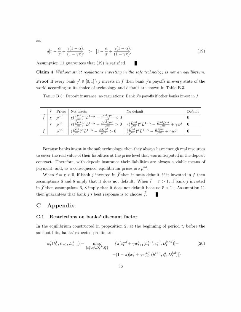
as:

q[r − α

π+γ(1− α)

(1− γπ)] > [1− α

π+γ(1− α)

(1− γπ)] (19)

Assumption 11 guarantees that (19) is satisfied.

Claim 4 Without strict regulations investing in the safe technology is not an equilibrium.

Proof If every bank j′ ∈ [0, 1] \ j invests in f then bank j’s payoffs in every state of the

world according to its choice of technology and default are shown in Table B.3.

Table B.3: Deposit insurance, no regulations: Bank j’s payoffs if other banks invest in f

r Prices Net assets No default Default

f r pnd r(Dnd

pnd)αL1−α − RndDnd

pd< 0 0

r pnd r(Dnd

pnd)αL1−α − RndDnd

pnd> 0 r(D

nd

pnd)αL1−α − RndDnd

pnd+ γwj 0

f pnd (Dnd

pnd)αL1−α − RDnd

pnd> 0 (D

nd

pnd)αL1−α − RDnd

pnd+ γwj 0

Because banks invest in the safe technology, then they always have enough real resources

to cover the real value of their liabilities at the price level that was anticipated in the deposit

contract. Therefore, with deposit insurance their liabilities are always a viable means of

payment, and, as a consequence, equilibrium prices are pnd.

When r = r < 0, if bank j invested in f then it must default, if it invested in f then

assumptions 6 and 8 imply that it does not default. When r = r > 1, if bank j invested

in f then assumptions 6, 8 imply that it does not default because r > 1 . Assumption 11

then guarantees that bank j’s best response is to choose f .

C Appendix

C.1 Restrictions on banks’ discount factor

In the equilibrium constructed in proposition 2, at the beginning of period t, before the

sunspot hits, banks’ expected profits are:

wjt (ht1, it−1, D

bt−1) = max

xkt ,skt ,Db,kt ,ikt

π[xndt + γwjt+1(ht+11 , indt , D

b,ndt )]+ (20)

+(1− π)[xdt + γwd,jt+1(ht+11 , idt , D

b,dt )]

36

s.t. xndt + sndt ≤ f(it−1, L)− Rt−1Dt−1

pt(21)

xdt + sdt ≤ f(it−1, L) (22)

ptindt ≤ D

b,ndt + pts

ndt (23)

ptidt ≤ D

b,dt + pts

dt (24)

where xkt , k = d, nd denotes time t consumption of bank j in default and no default;

similarly skt denotes savings, ikt investment into the productive technology and Db,kt deposits

offered57. Under assumption 7 a solution to problem (20) is such that sndt = 0.

D Appendix

D.1 Banks and Firms

This appendix provides a modified version of the model of section 2 to allow for banks

to make nominal loans to firms rather than owning productive projects directly, and for

banks to strategically default. Even if this appendix deals only with the one period model,

the same characterization applies to the dynamic model of section 3 for the involuntary

defaults.

None of the results in the paper change qualitatively: different partitions of the state

space would have to be assumed in propositions 1-4 and every result goes through. There-

fore, in the main body of the paper a simpler model where banks and firms are consolidated

has been privileged.

Consider an economy populated by three types of agents: households, banks and firms.

They are identical within their type, there is a continuum [0, 1] of each and all live for one

period. Consumption goods are as in section 2, as well as preferences and endowments for

households and banks: the only difference for banks is that they are endowed with labor,

l, and a technology that uses labor to produce an input good z (this can be interpreted

as a loan). Let zb denote the output of good z produced by banks, then zb = F (l). As in

section 2, they are endowed with a technology that allows them to plant coconut and which

returns r per unit of coconut planted: households deposit coconut at banks, D which gives

rise to an obligation for banks to pay R units of coconut to households at the end of the

period.

57Because this paper does not focus on coordination failures on the side of depositors, banks’ ability topay households for deposits they made in the previous period, is independent of deposits households makein the current period. This can be seen from (21) and (22) where banks do not have resources availablefrom current period deposits (Db,k

t ) to pay for their obligations (Rt−1Dt−1).

37

Firms’ preferences are linear in both the consumption of cash and credit goods: V f (cf1 , cf2) =

cf1 + cf2 . Firms are endowed with a technology f(z) that uses the input good to produce

either cash or credit goods: let zf denote the input of good z firms choose to invest into

production.

There is free entry into banking and there is a competitive market to trade good z that

opens at the beginning of the period, before the market for cash and credit goods opens,

where firms buy good z and banks sell good z at price pz. Then the goods’ market opens,

where firms can sell the output of cash and credit goods from their productive technology

at price p: they are paid wither with coconut or with bank-issued liabilities or both (as in

section 2).

Differently from section 2, at the end of the period firms have to settle with banks for

their purchases of good z made at the beginning of the period (firms have to pay back the

loan).

Then on this market so that their decision problems, respectively, are:

References

[1] N. Baba, S. Nishioka, N. Oda, M. Shirakawa, K. Ueda, and H. Ugai. Japan’s deflation

problems in the financial system and monetary policy. BIS working paper, No. 274,

March 2007.

[2] B. Bernanke. Nonmonetary effects of the financial crisis in the propagation of the

great depression. The American Economic Review, 73 No. 3:257–276, June 1983.

[3] B. Bernanke and M. Gertler. Financial fragility and economic performance. NBER

working papers series, No. 2318, July 1987.

[4] B. Bernanke and M. Gertler. Agency costs, net worth and business fluctuations. The

American Economic Review, 79 No. 1:14–31, March 1989.

[5] B. Bernanke, M. Gertler, and S. Gilchrist. The financial accelerator and the flight to

quality. The Review of Economics and Statistics, 78 No. 1:1–15, February 1996.

[6] C. Calomiris. Banking failures in theory and history: The great depression and other

”contagious” events. NBER Working Paper, N. 13597, November 2007.

38

[7] C. Calomiris and G. Gorton. The origins of banking panics. In Hubbard,R.Glenn,

Financial Markets and Financial Crises, pages 109–173. The University of Chicago

Press, 1991.

[8] C. Calomiris and J. R. Mason. Causes of us bank distress during the depression.

NBER Working Paper, N. 7919, September 2000.

[9] C. Calomiris and E. N. White. The origins of federal deposit insurance. In Goldin,

Claudia and Gary D. Libecap, The Regulated Economy, pages 145–188. The University

of Chicago Press, 1994.

[10] C. T. Carlstrom and T. Fuerst. Agency costs, net worth and business fluctuations: A

computable general equilibrium analysis. The American Economic Review, 87 No. 5,

1997.

[11] V. V. Chari. Banking without deposit insurance or bank panics: Lessons from a model

of the u.s. national banking system. Federal Reserve Bank of Minneapolis, Quarterly

Review, 13 No. 3, Summer 1989.

[12] V. V. Chari, L. Christiano, and M. Eichenbaum. Inside money, outside money, and

short-term interest rates. Journal of Money, Credit and Banking, 27 No. 4 Part

2:1354–1386, November 1995.

[13] V. V. Chari and R. Jagannathan. Banking panics, information, and rational expecta-

tions equilibrium. Journal of Finance, 13 No. 3 Part 2:749–761, July 1988.

[14] H. L. Cole and L. E. Ohanian. Deflation and the international great depression: A

productivity puzzle. Federal Reserve Bank of Minneapolis Research Department Staff

Report, February 2005.

[15] D. Diamond and P. Dybvig. Bank runs, deposit insurance and liquidity. Journal of

Political Economy, 91:401–19, June 1983.

[16] D. Diamond and R. Rajan. Money in a theory of banking. American Economic

Review, 96:30–53, 1 2006.

[17] H. Ennis and T. Keister. Commitment and equilibrium bank runs. Federal Reserve

Bank of New York Staff Report, N. 274, March 2007.

39

[18] I. Fisher. The debt-deflation theory of the great depression. Econometrica, 1 No.

4:337–357, October 1933.

[19] M. Friedman and A. J. Schwartz. A Monetary History of the United States, 1967-1960.

Princeton University Press, 1963.

[20] G. Gorton. Banking Panics and Business Cycles. Oxford Economic Papers, 40, 1988.

[21] E. J. Green and P. Lin. Implementing efficient allocations in a model of financial inter-

mediation. Federal Reserve Bank of Minneapolis Research Department Staff Report,

109:1–23, 2003.

[22] R. E. Lucas and N. L. Stokey. Optimal fiscal and monetary policy in an economy

without capital. Journal of Monetary Economics, N.12:55–93, 1983.

[23] R. E. Lucas and N. L. Stokey. Money and interest in a cash-in-advance economy.

Econometrica, 55, N.3:491–513, May 1987.

[24] A. Martin. Liquidity provision vs deposit insurance: preventing bank panics without

moral hazard. Economic Theory, 28:197–211, 2006.

[25] G. Richardson. The check is in the mail: correspondent clearing and the collapse of

the banking system, 1930 to 1933. The Journal of Economic History, 67 N. 3:643–671,

September 2007.

[26] O. Sprague. History of Crises Under the National Banking System. Report by the

National Monetary Commission to the U.S. Senate. 61st Cong., 2nd sess., S. Doc. 538,

Government Printing Office, Washington, D.C, 1910.

[27] C. Warburton. Monetary expansion and the inflationary gap. American Economic

Review, 34:303–327, 2 Part 1 1944.

[28] C. Warburton. Monetary theory, full production and the great depression. Economet-

rica, 13 N. 2:114–128, 1945.

[29] C. Warburton. Quantity and frequency of use of money in the united states, 1919-45.

The Journal of Political Economy, 54 N.5:436–450, 1945.

[30] C. Warburton. The volume of money and the price level between the world wars. The

Journal of Political Economy, 53 N. 2:150–163, 1945.

40

[31] G. F. Warren and F. A. Pearson. Prices. New York: John Wiley, 1933.

[32] E. N. White. The legacy of deposit insurance. In Bordo, Michael D., Claudia Goldin

and Eugene White, The Defining Moment, pages 87–124. The University of Chicago

Press, 1998.

[33] E. Wicker. The Banking Panics of the Great Depression. Cambridge University Press,

1996.

41