RESEARCH ARTICLE An overview of various new road pro le ...louisgagnon.com/articleArchive/LouisGagnon_gPAV_finalSubmission.pdf · A steering algorithm similar to the moment-by-moment

April 11, 2014 19:10 International Journal of Pavement Engineering LouisGagnon˙gPAV

International Journal of Pavement EngineeringVol. 00, No. 00, Month 2013, 1–24

RESEARCH ARTICLE

An overview of various new road profile quality evaluationcriteria : part 1

Louis Gagnon,a∗ Guy Dore,b

and Marc J. Richarda

aDepartment of Mechanical Engineering, Laval University, Quebec, QC, Canada;bDepartment of Civil Engineering, Laval University, Quebec, QC, Canada

(Submitted for review)

A multibody tractor-trailer model specialised in measuring the impact of roadsurface quality on the efficiency of transport was developed. It was calibratedand validated using a coastdown tests experimental campaign. The model wasthen used within an extensive profile study that linked specific profiles to theirimpact on energy consumption, vehicle wear, driver and passenger health, andsafety. Two hundred and seventy 1 km long profiles were tested with the multi-body vehicle travelling at 100 km/h. It allowed to identify trends in the re-lationships between various profile rating criteria and the impacts aforemen-tioned. The criteria consist of 19 indices observed on a quarter car model op-erating on longitudinal road profiles. They yield accurate predictions of profileimpacts. For the operating conditions considered, the long wavelengths have astrong effect on health, medium wavelengths on safety, and short to mediumwavelengths on energy consumption.

Keywords: road roughness; IRI; quarter car; fuel efficiency; safety; health; multibodydynamics )

1. Introduction

The smoothness of the road surface has an undeniable influence on vehicle efficiency andpoor roads incur a cost to vehicle operators. A thorough literature review lead Gagnonet al. (2006) to conclude that vehicle efficiency decreases when the road deteriorates. Thenegative consequences of a poor road surface quality can be broken down in differentcategories: fuel consumption (Velinsky and White 1980, Wambold 1985, Delanne 1994,Gyenes and Mitchell 1994, McLean and Foley 1998, Jackson 2004, Miege and Popov

∗Corresponding author. Email: [email protected]

ISSN: 1029-8436 print/ISSN 1477-268X onlinec⃝ 2013 Taylor & FrancisDOI: 10.1080/1029843YYxxxxxxxxhttp://www.informaworld.com


2 L. Gagnon, G. Dore, and M. J. Richard

2005, Fraggstedt 2006, Rhyne and Cron 2007, Jackson et al. 2011); driver and passengerwellness (Bouazara 1997, Fichera et al. 2007); and, safety (Sattaripour 1977, Bester2003, Romao et al. 2003, Vassev 2005, Richard et al. 2009). The importance of thosethree impact categories has been outlined by the World Health Organization in variousreports. For example, road traffic incidents are the eighth leading cause of mortalitytoday (WHO 2013), gas emissions from vehicles give rise to pulmonary diseases which arealso amongst the leading causes of death (WHO 2011), and low back pain is the majorcause of morbidity worldwide (WHO 2002) and, coincidently, is widespread amongstheavy equipment operators.Bearing that in mind, agencies responsible for the construction and maintenance of

roads usually monitor the longitudinal profiles of their roads by taking profilometerreadings. Although such readings are now standard procedure in developed countries,they usually only serve to compute the International Roughness Index (IRI). This indexis widely used and is a calculation of the accumulated suspension movement of theReference Quarter Car Simulation travelling at 80 km/h on the given profile. Typically,a road is considered to be in a splendid state when the IRI is between 1.0 and 1.5 m/kmand in a horrible state when the IRI is above 5 m/km. For example, Pehlivanidis andSt-Laurent (2001) report that, in 1999, the national roads of Quebec had an average IRIof 2.1 m/km while the collector roads had an average IRI of 3.1 m/km.Hence, a semitrailer truck multibody model has been developed and validated in order

to establish a precise link between a profile and its consequences. Fifty-four real 1 kmlong road profiles provided by Quebec’s ministere des Transports (MTQ) were analysed.They were taken from the up to date road database of the MTQ and selected in order toinclude from the smoothest to the worst road profiles. Each of these was used to generate4 filtered profiles isolating the short, medium, long, and IRI wavelengths, thus yielding atotal of 270 profiles. These filtered profiles derived from real ones are not likely to occurin real life but can trigger responses useful for research purposes. The truck model wasdriven in a straight line on each profile at a constant velocity of 100 km/h. This articlepresents the impact-index relations obtained and the trends identified after running themodel on these 270 road profiles. It is the first of a two part article where the secondpart will cover the road impact on vehicle wear, a profile wavelength analysis method,and the particulars of the multibody model.

2. Methodology

This section summarises the approach taken to model the vehicle, run it on a profile,evaluate the impact from the road surface quality, and characterise the different profiles.

2.1. Multibody model

The multibody approach is the preferred choice of many authors when it comes to eval-uating the aspects of energy consumption (Velinsky and White 1980, Lu 1985, Ficheraet al. 2007, Stenvall 2010, Hammarstrom et al. 2012), occupant wellness (Bouazara 1991,1997, Rakheja et al. 2001), and safety (Kollman 2007, Imine 2007). It was chosen toimplement the model into the free and open-source software MBDyn (Masarati 2012,Masarati et al. 2014).


International Journal of Pavement Engineering 3

2.1.1. Tractor semitrailer

The semitrailer truck is implemented as a multibody model. It has 331 degrees offreedom (DoF) including the tyres. The chosen tractor is a conventional cab FreightlinerCascadia R⃝ and it tows a 16.2 m long three axle Manac R⃝ semitrailer. The total vehicleweight is 43 t. Apart from the wheels, the model has 13 rigid bodies having each 6 DoF :one for each axle; one for the chassis frame and the components which are rigidly attachedto it, such as the batteries and gas tanks; one for the engine; one for the cabin; one for thedriver and one for the passenger; one for the radiator; and, one for the semitrailer frame.The tractor and trailer are tied together by a spherical joint. The radiator is attached tothe chassis by 2 uncoupled translational tridimensional viscoelastic elements. It is alsoconstrained to prevent rotation about the tractor lateral axis by a cardano rotation joint,which is equivalent to two revolute joints placed orthogonal to each other. A side-viewof the multibody truck model is shown in Figure 1

z

x

Figure 1. Sideview of the tridimensional truck model.

A steering algorithm similar to the moment-by-moment feedback models of Blundelland Harty (2004) is implemented. Its goal is to follow a straight line. The algorithmcomputes an error function which then gives a desired steering angle according to userset aggressivity factor and visibility distance parameters. This angle is then applied tothe front wheels by an orientation constraint on their vertical axis.Aerodynamic drag is accounted for by forces acting on the cabin and on the semitrailer

in their longitudinal directions. It uses a calibrated truck drag coefficient to compute thedrag force of which 55% acts on the cabin and 45% on the semitrailer, as derived fromthe data provided by Drollinger (1987).Parasitic losses, which are the losses incurred by the wheel hub bearings, are applied

as constant forces in the longitudinal direction of each axle.Losses in the differential and in the transmission are used for the coastdown validation

runs. They are applied as forces in the longitudinal direction of the two drive axles andthey are calculated using a method given by Hammarstrom et al. (2012).The complete tractor trailer model was calibrated and validated from the data ob-

tained during an experimental campaign of coastdown tests where each run was repeated5 times. Two sections of 518 m and 714 m lengths taken on an 80 km/h service roadwere tested in both directions thus resulting in 4 test segments. The segment’s IRI variedbetween 5.9 m/km and 8.2 m/km and the individual track IRI varied between 5.1 m/kmand 9.8 m/km, these are degenerate surface conditions. Such a high level of deteriora-tion was chosen to ensure that the model is validated against road profiles that have astrong influence on the response of the vehicle. For the campaign, the procedure recom-mended by the J2263 norm (SAE 2008) was closely followed. Fourteen truck parameterswere optimised to reproduce the experimental wheel-by-wheel weight distribution. Then,the calibration was carried on by adjusting the 40 acceleration curves and the 4 kinetic



energy loss calculations to the experimental data by adjusting another 16 model parame-ters consisting of the horizontal position of the semitrailer’s center of mass and the staticdeflection of each suspension.

2.1.2. Multibody tyres

It was chosen to implement a rigid ring tyre model as a modification of the model ofGualdi et al. (2008) which was available in MBDyn. The implemented model is based onthe Short Wavelength Intermediate Frequency Tire (SWIFT) model presented by Pacejka(2006) and it filters the road input using the method of Schmeitz (2004). The tyre modeltakes the three-dimensional forces and moments coming from the wheel of the truckmodel as one input (Gagnon et al. 2012). The other input to the tyre model is the roadprofile height. Its equations are implicitly integrated at each time step and the rotationparameters are handled by the updated-updated approach defined by Masarati (2000).A simplified physical interpretation of the model is shown in Figure 2. It has three rigid

elements. The inner element is referred to as the Wheel and comprises the wheel and anyrotating mass attached to it, including a portion of the tyre sidewall, and is connectedto the vehicle as a wheel hub assembly and allowed to roll. The outer element is referredto as the Ring and represents part of the sidewall, the belt, and the tread of the tyreand its purpose is to simulate the inertia of a rotating tyre. The external rigid elementis a point mass referred to as the Patch and represents the translational inertia of theportion of the tread which exchanges friction and constraining forces with the ground.There are three independent translational viscoelastic elements that link the Wheel tothe Ring and three that link the Ring to the Patch. There are also three independenttorsional viscoelastic elements that link the Wheel to the Ring. The viscoelastic elementsare implemented as noted by Masarati and Morandini (2010). The Patch is not subjectedto gravity. Its height is dictated by its longitudinal position on the road and its verticalvelocity is determined from its longitudinal velocity and the slope of the road profile.Slip forces obtained by the empirical formulae published by Pacejka (2006) are appliedon the Patch.

Wheel

Ring

Patch

Figure 2. From left to right: Wheel, Ring, and Patch elements.

The calculated response of the tyre is precise for perturbation frequencies up to 100 Hzand for road protuberances up to 10 cm in height. It takes 45 tyre parameters and20 algorithm parameters. The numerical integration is done implicitly except for theroad profile data which uses data at the previous time step. The model was calibratedand validated by comparison to finite element analysis results provided by Michelin R⃝ forXZA-3 tyres assembled on a wheel attached to an axle and travelling over rectangularcleats. Above 20 km/h, the coefficient of determination R2 was greater than 0.8 for all



vertical cleat force responses. As for the longitudinal forces, only one curve had a R2

below 0.5.

2.2. Profile evaluation procedure

A profile evaluation study was conducted by using the developed truck model and runningit at 100 km/h in a straight line on longitudinal road profiles. More than 200 one kilometrelong profiles measured at 25 mm intervals were analysed. They represented paved roadsof smoothness ranging from excellent to mediocre were analysed. In order to assess thefull impact of the profile and nothing else, steps were taken to ensure that the vehiclewas in equilibrium before entering and after leaving a profile. For the profile study, thetruck velocity was controlled by an explicit cruise control algorithm which applies thesame torque to each of the 8 drive wheels. The torque applied is function of the differencebetween targeted and actual vehicle velocities. It produces a maximum power of 274 kWwhich accounts for a 10% loss in the transmission.

2.2.1. Impact assessment

The three aforementioned impact categories are evaluated by examining the resultsof the multibody model runs. First, the quantity of energy qtot that a particular profiledissipates is calculated from the following equation,

qtot =

8∑i=1

(∫ xout

xin

ωiτidt

)+∆Ekmck +∆Epmcp (1)

where ωi and τi are the angular velocity and torque applied to wheel i. The integral istaken on the profile section considered and mck and mcp are the masses of the truck usedfor the kinetic and potential energy calculations, respectively. The variable ∆Ep is thequantity of potential energy per kilogramme that was lost on the profile and is calculatedby the following equation,

∆Ep = (zfra,in − zfra,out) g (2)

where zfra,in and zfra,out are the respective vertical elevations of the truck frame at thestart and at the end of the section considered and g is standard gravity. The lost kineticenergy per kilogramme ∆Ek is calculated from the following equation,

∆Ek =x2fra,in − x2fra,out

2(3)

where xfra,in and xfra,out are the respective velocities of the truck frame at the start andend of the section considered.Now, human impact is evaluated using the acceleration versus time signals treated

according to the 2631-1 norm from the for Standardization (1997). For each humanimpact category and for the different calculation methods, the norm specifies the propersignals to use, filters and weightings to apply, and summation methods to rely on. In theend, the health hazard is measured by the Root Mean Square (RMS) of the treated signal.Table 1 reveals which signals are used for each measure presented here. The conservativemeasure only considers the vertical acceleration signal under the seat and uses Eq. (4) if



Table 1. Signals used to evaluate the different profile induced human im-pacts.

Criteria Seat translation Seat rotation Backrest FeetWithout backrest x,y,zWith backrest x,y,z xConservative z

Comfort x,y,z x,y,z x,y,z x,y,zNausea z

that signal has a crest factor above 9. Also, where 4th power is specified, the RMS valueaw is replaced by the following equation,

aw =(∑

a4wi

)1/4(4)

where a4wi is the frequency weighted acceleration signal. The crest factor is defined by thenorm as the ratio of the maximum instantaneous magnitude of the filtered signal overits RMS value.At last, safety is evaluated by individually observing the evolution of the normal force

under each tyre. The criteria considers the average distance travelled by each tyre witha tyre normal force below a given threshold. That threshold is a percentage of what thenormal force would be if the truck were circulating on a perfectly smooth road. The2 front wheels are considered separately from the others because they are crucial andless sensitive to the profile. They thus turn out to be a conservative result. The distancedsaf,i travelled by the truck with a wheel i with a force below the threshold is measuredfor each wheel according to the following equation,

dsaf,i =∑j

bi,jxcab,j+1 − xcab,j−1

2(5)

where bi, j is a boolean expression which is equal to one if and only if the normal forceof wheel i at time j is below the threshold and xcab,j±1 is the cabin position at timestepj ± 1. The criteria is the average value of dsaf,i taken over either the two front wheels orthe twenty rear wheels.

2.2.2. Road profile rating

Various existing methods provide the means to rate roads by examining their longitu-dinal profiles. Some of these methods along with improved ones are presented, studied,and discussed.First of all, the IRI is the most widely used method and is based on the Reference Quar-

ter Car Simulation which uses the parameters of the golden car (Sayers and Karamihas1998). The accumulated vertical movement of the golden car ’s suspension when travel-ling at 80 km/h constitutes the IRI and has units of distance of vertical movement overdistance travelled. The golden car is used for all the indices presented in this article.That said, the HRI is the IRI calculated using the average of the left and right trackroad profiles instead of being calculated using each track and then averaged. These twoindices are presented in detail by Sayers and Karamihas (1998). Then, the FRI is iden-tical to the HRI except that it takes the average profile elevation over 4 points instead



Table 2. Wavelength range breakdown of the various profile setsconsidered.

Profile set Range (m) Profile description QtyMTQ [0.00, 91] Reala, provided by MTQ 54

Short (S) [0.707, 2.83] Bandpass filteredb 38

Medium (M) [2.83, 11.3] Bandpass filteredb 38

Long (L) [11.3, 45.2] Bandpass filteredb 38

IRI (I) [0.25, 91] Bandpass filteredb 38

Qualified (Q) [0.00, 91] Realb, provided by MTQ 38All (A) Various Real and filteredc profiles 233

aTwo of the real profiles were constructed from the foward and back-ward repetition of a particularly irregular 91 m section taken froma profile.bThese categories only include profiles and their filtered derivativeswhich converged for every bandpass filtering presented.cAs opposed to the bandpass filtered profiles, this category includesevery profile which converged without regard for their filtered deriva-tives.

of 2 and these points are chosen as the horizontal positions of the four wheels of a typicalcar. This index thus uses a typical passenger car wheelbase distance of 2.616 m. A truckwheelbase was avoided because the purpose is to have an index which can be used forall vehicles.These three indices were calculated for the official MTQ profiles, which are only filtered

by a high-pass filter at 91 m. Then, they are also calculated for the same MTQ profilesfiltered in a way to isolate three different bandwidths. These bandwidths are: 1) theshort wavelengths, from 0.707 m to 2.83 m; 2) the medium wavelengths, from 2.83 mto 11.3 m, 3) the long wavelengths, from 11.3 m to 45.2 m. In order to avoid a phasedelay, two 3rd order Butterworth filters were applied sequentially on the forward andreversed signals. These bandwidths are established by researchers (Martel et al. 2011)who are able to predict the effect a specific road restoration procedure will have on eachof the bandwidths. The various profile categories presented in this paper are made clearin Table 2.Pushing the index development slightly further a Health Index based on the ISO-2631-

1 guidelines was developed. It is defined as the RMS value of the weighted accelerationof the suspended mass of the golden car . It uses the conservative approach describedearlier in Section 2.2.1.A Wear Index is also developed. It yields a value DGC which is equivalent to the

damage accumulated by the suspension of the golden car . It is computed by the followingequation,

DGC =∑j

((2am,j)3nam,j

) (6)

where am is the acceleration of the quarter car’s suspended mass, am,j is the magnitudeof the acceleration am for which nam,j

cycles occur in the signal. Those 2 variables areobtained by a rainflow counting algorithm. These two indices are also measured on 2 and4 points average profiles in the same fashion as for the HRI and FRI.Finally, another index is implemented and is called the Safety Index. It is obtained by

calculating the distance per kilometre of profile for which the spring representing the tyre



of the quarter car is stretched above a chosen threshold of 1.75 cm. It is only calculatedon the original MTQ profile.In order to clarify the 19 different indices which were just presented, Table 3 describes

each of them individually. There, the term simple refers to indices which are presentedas an average index between the left and right road tracks. The detailed calculation ofeach index is presented in Section A. The distribution of the profiles referred to as theQualified profiles covers the range of IRI from very small at 0.68 m/km to quite largeat 7.6 m/km. This is seen on Figure 3 which gives an insight on the range of indicestested and how they relate to each other by linking each index value to the value of thesame profile for the other indices. The figure also shows that these profiles are evenlydistributed in terms of Short Waves, Medium Waves, and Long Waves IRI. Conversely,the the Health, Wear, and Safety indices show some extreme values. Finally, the figureshows that strong Health and Wear indices are associated with a strong IRI and thatthe Health and Safety indices are closely related.

0

2

4

6

8

10

12

IRI SW IRI MW IRI LW IRI SI HI WI1/4

Value

Index

Figure 3. Distribution of the 38 Qualified profiles’ IRI, short wave IRI (SWIRI), medium waveIRI (MWIRI), long wave IRI (LWIRI), Safety Index (SI), Health Index (HI), and the fourthroot of the Wear Index (WI1/4). The lines connecting the values have the purpose of linking thevarious indices of a same profile together.

Apart from being used to evaluate the indices, the filtered profiles are also used torun the full truck model. The purpose of doing so is to isolate the impacts that differentbandwidths have on the vehicle. Furthermore, a supplementary bandpass filter is used



Table 3. The indices evaluated in this study.Name Units DescriptionSimple Health Indexa m/s2 weighted acceleration of the suspended mass of the golden

carIRI m/km International Roughness IndexShort Waves IRI m/km IRI of a filtered profile which retains the short wavelengthsMedium Waves IRI m/km IRI of a filtered profile which retains the medium wave-

lengthsLong Waves IRI m/km IRI of a filtered profile which retains the long wavelengthsSimple Wear Indexa N3 · cycles accumulated damage by the golden car suspensionTwo point Health Indexa m/s2 weighted acceleration of the suspended mass of the golden

car circulating on the average profile of the left and righttyre tracks

HRI m/km IRI of the average profile of the left and right tyre tracksShort Waves HRIa m/km HRI taken on a profile which was first averaged between

left and right tyre tracks and then filtered to retain theshort wavelengths

Medium Waves HRIa m/km HRI taken on a profile which was first averaged betweenleft and right tyre tracks and then filtered to retain themedium wavelengths

Long Waves HRIa m/km HRI taken on a profile which was first averaged betweenleft and right tyre tracks and then filtered to retain thelong wavelengths

Two point Wear Indexa N3 · cycles accumulated damage by the golden car suspension cir-culating on the average profile of the left and right tyretracks

Four point Health Indexa m/s2 weighted acceleration of the suspended mass of the goldencar circulating on the average profile of the left and righttyre tracks of the front and rear axles of a typical car

FRIa m/km IRI of the average profile of the left and right tyre tracksof the front and rear axles of a typical car

Short Waves FRIa m/km FRI taken on a profile which was first averaged betweenleft and right tyre tracks of the front and rear axles ofa typical car and then filtered to retain the short wave-lengths

Medium Waves FRIa m/km FRI taken on a profile which was first averaged betweenleft and right tyre tracks of the front and rear axles of atypical car and then filtered to retain the medium wave-lengths

Long Waves FRIa m/km FRI taken on a profile which was first averaged betweenleft and right tyre tracks of the front and rear axles of atypical car and then filtered to retain the long wavelengths

Four point Wear Indexa N3 · cycles accumulated damage by the golden car suspension cir-culating on the average profile of the left and right tyretracks of the front and rear axles of a typical car

Simple Safety Indexa m/km total distance for which the golden car tyre spring isstretched beyond a given threshold

aIndex particular to this paper.

for the truck model. It is called the IRI filter and has a range of 250 mm to 91 m. It waschosen because such a filter is used in the standard IRI method. However, the developedtruck model has a sensitive tyre model which has no need of the tyre filtering intendedby the 250 mm low-pass filter.



3. Results and trends identified

This section summarises the trends that are obtained after testing every possible impact-index relation. To avoid redundancy, the bandpass filtered roughness indices are nottaken on filtered profiles. When denoted as such, the curves have been normalised. Thenormalisation consists of plotting the results in terms of number of times of impactincrease with respect to the lowest impact value recorded on the curve.Most impact trends are presented by a correlation with a first degree polynomial having

the form f(x) = ax + b which are referred to as linear correlations. Some trends arehowever presented using a second degree polynomial having the form f(x) = ax2+ b andthey are referred to as quadratic correlations. Higher order two-term polynomials weretested but did not yield better coefficients of determination.Of the 270 profiles evaluated, the truck model converged for 233 of them. These 233 pro-

files are the ones referred to as All in Table 2. For consistency amongst different wave-lengths, the 38 profiles shown as unfiltered or bandwidth filtered profiles are only theones which converged for both the original and bandwidth filtered profile variants.

3.1. Energy

The best energy correlation came with the Simple Health Index and is shown on Figures 4and 5. The quadratic correlation was of an equal coefficient of determination and theSimple Health Index gave the best correlation obtained amongst all indices for both linearand quadratic correlations. The two point Health Index gave the best cubic correlationwith a R ∼ 0.89. The Safety Index was also found to give a very good correlation (R ∼0.91). It was found that long wavelengths have a very limited influence. Furthermore, theMedium Waves roughness indices correlated better with energy consumption by reachinga quadratic correlation of R ∼ 0.73 with a tipping point at the value of 3 m/km. Theresults also highlight the fact that the regular IRI is unable to precisely predict energyconsumption, as its coefficient of determination with fuel consumption was R < 0.4.Another fact worth noting is the presence of the two profiles generated by cycling inthe forward and reverse directions of a subsection of a real profile. This particular profileseverely excited the truck and produced an 80% energy consumption increase. It changedthe correlation values for most of the indices in a way that made the Safety Index thebest predictor by far when this profile was considered.The results of Figure 4 agree well with what has been reported by Wambold (1985)

who mentions that it is at excitation frequencies between 5 Hz and 20 Hz that most ofthe energy is dissipated in the vehicle. At 100 km/h those frequencies correspond to abandwidth range of 1.7 m to 5.6 m which spans the short and medium wavelength rangepresented here. At last, Figure 5 shows how little impact the IRI filtering has on thecalculated energy consumption. Thus, when Hammarstrom et al. (2012) mention thatwavelengths between 5 mm and 0.5 m have a strong influence on vehicle energy con-sumption, wavelengths between 50 mm and 0.25 m can probably be excluded from thatstatement. This exclusion is justified because that range is the only difference betweenthe Qualified and IRI profiles presented on Figure 5. Indeed, the IRI filter removes any-thing below 0.25 m and both profiles exclude anything below 50 mm due to the 25 mmsampling interval used by the MTQ.



0

0.05

0.1

0.15

0.2

0.25

0.3

0.35

0 1 2 3 4 5 6 7

Energy(J)

Simple Health Index (m/s2)

S, R2 = 0.824M, R2 = 0.933L, R2 = 0.434I, R2 = 0.904

Figure 4. Linear correlations of normalised energy consumption against the Simple Health Indexfor short (S), medium (M), long (L) and IRI (I) wavelengths filtered profiles.

0

0.02

0.04

0.06

0.08

0.1

0 0.5 1 1.5 2

Energy(J)


Q, R2 = 0.909I, R2 = 0.904

Figure 5. Lower portion of the linear correlations of normalised energy consumption against theSimple Health Index for Qualified (Q) and IRI (I) wavelengths filtered profiles.

3.2. Health issues

The best correlation between the impact of road roughness on the driver health and theLong Waves FRI is shown on Figure 6. As expected, the Long Waves IRI and Long WavesHRI also yield very good correlations with coefficients of determination R2 ∼ 0.9. Theother indices and wavelengths, both linear and of higher order, give correlations withcoefficients R2 < 0.5. The best multi wavelength correlation comes from the FRI and itis shown on Figure 7. It clearly shows that long wavelengths have the most importantimpact on driver health while the medium and short wavelengths have low and negligibleimpacts, respectively.In order to get more elaborate information on the health impact, selected relationships

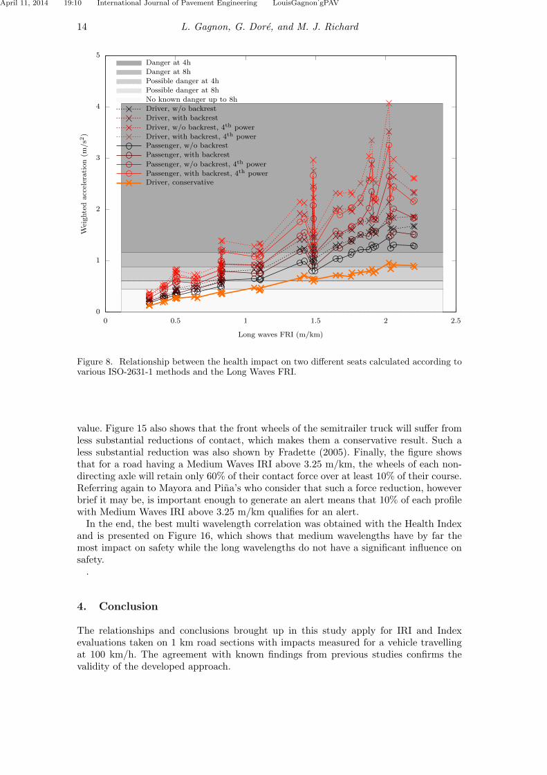
obtained by applying the ISO-2631-1 norm to the results of the Qualified profiles arepresented. Of these, the Long Waves FRI is shown on Figure 8. Although coming shortof expectations by presenting a more chaotic correlation, the Health Index is neverthelessshown on Figure 9. Both figures show that the conservative measure warns of a benignimpact when compared to the less conservative methods. In fact, when the 3 vibrationsin translation at the seat and the 3 at the backrest are considered, the measured impacton health more than doubles. Being even less conservative, the health impact measured



-0.2

0

0.2

0.4

0.6

0.8

1

0 0.5 1 1.5 2 2.5 3Weightedacceleration(m

/s2)

Long Waves IRI (m/km)

R2 = 0.897

D.8hP.4hP.8h

No.8h

Figure 6. Linear correlation between the conservative impact on driver health and the LongWaves IRI with delimiters for zones of danger (D), possible danger (P), and no danger (No) aftercontinued daily exposures of 4h and 8h.

on the signal processed by the 4nd degree power mean of Eq. (4) and using backrestvibrations will be roughly 4 times greater than the conservative measure. The resultsdisplayed here and the profiles of Figure 3 highlight the fact that the Health Index doesnot correlate with the IRI as the RMSA index presented by Sayers and Karamihas (1998)did. The possible explanation is that although both indices measure the RMS accelerationof the golden car , only the Health Index applies a frequency weighting to the seat signal.Comfort showed good correlations with the IRI, HRI, and FRI whether they were

filtered by bandpass filters or not. The relationship with Long Waves IRI is shown onFigure 10 where it is clear that the ride may be extremely uncomfortable and is at leastvery uncomfortable as soon as the Long Waves IRI reaches 2 m/km. If only the IRI isconsidered, the ride will be very uncomfortable at 4 m/km and extremely uncomfortableabove 5 m/km. Comfort measured using the non-conservative power mean from Eq. (4)on the accelerations signals shows a more abrupt response by emphasising the measuredimpact of a brief perturbation. Whether occupants most dislike short and strong impactor repeated weaker impacts remains subjective. Also, Figures 8 to 10 show by the dif-ference between driver and passenger that their seat adjustments and position in thevehicle have an observable impact on occupant health and comfort.Figure 11 shows that the Long Waves IRI gives an approximation of the percentage

of vehicle occupants that would suffer from a strong enough nausea to induce vomiting.Roughly one person out of twenty-five will be sick after circulating more than 6 h on aroad with a Long Waves IRI greater than 2 m/km. The quality of the correlation withlong wavelengths confirms that they are the most likely to cause nausea.

3.3. Safety

The Safety Index gives the best correlation for both All and Qualified profile sets. Bothcorrelations appear on Figure 12 The Safety Index allows to join the data points thatwould otherwise seem to deviate from the mean. A 2nd degree curve would give a cor-relation of R2 = 0.93 with All profiles. Conversely, the Four point Health Index whichgives a very good safety correlation with the Qualified profiles at R2 = 0.89 has a poorcorrelation with R2 = 0.20 when All profiles are considered. This is due to the presenceof two extreme profiles which seem to strongly excite a natural frequency of the vehicle.



0

0.2

0.4

0.6

0.8

1

0 1 2 3 4 5

Weightedacceleration(m

/s2)

FRI (m/km)

Danger at 8h

Possible danger at 4h


No known danger up to 8h

250mm - 91m, R2 = 0.866

Short wavelengths, R2 = 0.335

Med. wavelengths, R2 = 0.384

Long wavelengths, R2 = 0.862

Figure 7. Linear correlations between conservative impact on driver health and the FRI withdelimiters for zones of danger, possible danger, and no danger after continued daily exposures of4h and 8h.

The medium wavelengths roughness indices all yield reasonable correlations for a 2nd

degree curves, as shown for the Medium Waves HRI on Figure 13 where only the lowrange portion of the correlation is displayed. Finally, the relationship between IRI andsafety is presented on Figure 14 where criteria values are truncated at a 3 m accumulatedloss of contact distance. The figure allows to state that for IRI above 3 m/km, reductionsof more than 70% of the friction force available at the front tyres almost certainly occurwhile for IRI below 3 m/km, such reductions almost certainly do not occur. It also showsthat for IRI above 5.5 m/km there is most likely at least 2 m of accumulated distance of70% reduced friction force. These IRI relationships agree very well with previous findingsof Richard et al. (2009). The given distances on Figures 12 to 16 are the average distancesper tyre for which the truck will travel on the 1 km long profile studied with a normalforce equal or below 30% of the reference force.Safety is also plotted against various criteria. On Figure 15 the relations between

Medium Waves IRI and different levels of reduction of contact are shown. From thatfigure and the approach of Mayora and Pina (2009), it can be deduced that a profilealert should be generated when the MediumWaves IRI is above 1.5 m/km. Those authorsgenerate an alert for Sideway-force Coefficient Routine Investigation Machine (SCRIM)values between 0.6 and 0.5, which means a normal force below 60% of its undisturbed



0

1

2

3

4

5

0 0.5 1 1.5 2 2.5


/s2)

Long waves FRI (m/km)

Danger at 4h

Danger at 8h




Driver, w/o backrest

Driver, with backrest

Driver, w/o backrest, 4th power

Driver, with backrest, 4th powerPassenger, w/o backrest

Passenger, with backrest

Passenger, w/o backrest, 4th power

Passenger, with backrest, 4th powerDriver, conservative

Figure 8. Relationship between the health impact on two different seats calculated according tovarious ISO-2631-1 methods and the Long Waves FRI.

value. Figure 15 also shows that the front wheels of the semitrailer truck will suffer fromless substantial reductions of contact, which makes them a conservative result. Such aless substantial reduction was also shown by Fradette (2005). Finally, the figure showsthat for a road having a Medium Waves IRI above 3.25 m/km, the wheels of each non-directing axle will retain only 60% of their contact force over at least 10% of their course.Referring again to Mayora and Pina’s who consider that such a force reduction, howeverbrief it may be, is important enough to generate an alert means that 10% of each profilewith Medium Waves IRI above 3.25 m/km qualifies for an alert.In the end, the best multi wavelength correlation was obtained with the Health Index

and is presented on Figure 16, which shows that medium wavelengths have by far themost impact on safety while the long wavelengths do not have a significant influence onsafety..

4. Conclusion

The relationships and conclusions brought up in this study apply for IRI and Indexevaluations taken on 1 km road sections with impacts measured for a vehicle travellingat 100 km/h. The agreement with known findings from previous studies confirms thevalidity of the developed approach.



0

1

2

3

4

5

6

0 0.5 1 1.5 2 2.5 3 3.5 4 4.5


/s2)

Four point Health index (m/s2)

Danger at 4h

Danger at 8h




Driver, w/o backrest

Driver, with backrest

Driver, w/o backrest, 4th power

Driver, with backrest, 4th powerPassenger, w/o backrest

Passenger, with backrest

Passenger, w/o backrest, 4th power

Passenger, with backrest, 4th powerDriver, conservative

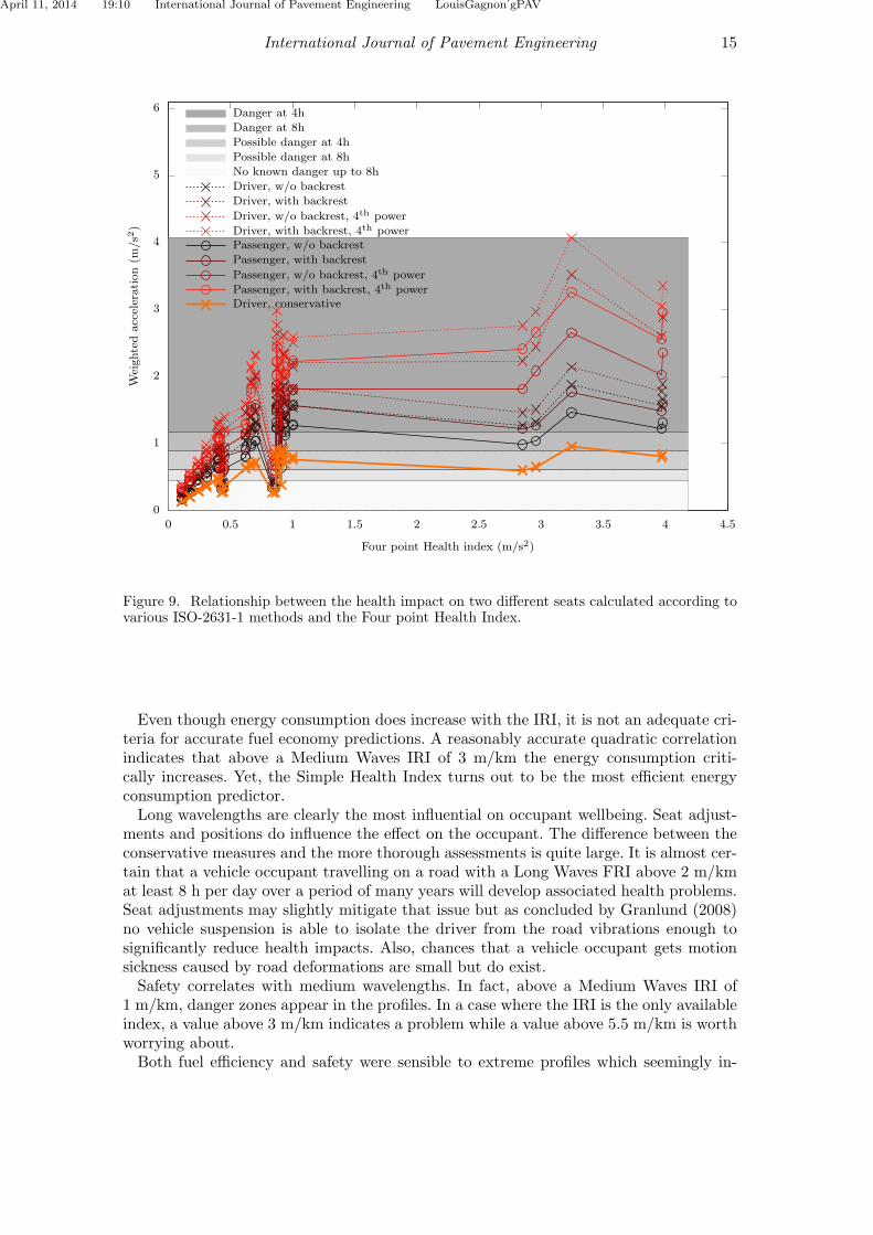
Figure 9. Relationship between the health impact on two different seats calculated according tovarious ISO-2631-1 methods and the Four point Health Index.

Even though energy consumption does increase with the IRI, it is not an adequate cri-teria for accurate fuel economy predictions. A reasonably accurate quadratic correlationindicates that above a Medium Waves IRI of 3 m/km the energy consumption criti-cally increases. Yet, the Simple Health Index turns out to be the most efficient energyconsumption predictor.Long wavelengths are clearly the most influential on occupant wellbeing. Seat adjust-

ments and positions do influence the effect on the occupant. The difference between theconservative measures and the more thorough assessments is quite large. It is almost cer-tain that a vehicle occupant travelling on a road with a Long Waves FRI above 2 m/kmat least 8 h per day over a period of many years will develop associated health problems.Seat adjustments may slightly mitigate that issue but as concluded by Granlund (2008)no vehicle suspension is able to isolate the driver from the road vibrations enough tosignificantly reduce health impacts. Also, chances that a vehicle occupant gets motionsickness caused by road deformations are small but do exist.Safety correlates with medium wavelengths. In fact, above a Medium Waves IRI of

1 m/km, danger zones appear in the profiles. In a case where the IRI is the only availableindex, a value above 3 m/km indicates a problem while a value above 5.5 m/km is worthworrying about.Both fuel efficiency and safety were sensible to extreme profiles which seemingly in-



0

1

2

3

4

5

6

7

0 0.5 1 1.5 2 2.5 3


/s2)

Long waves IRI (m/km)

Extremely

Very to extremely

Very

Actually to very

Actually

Fairly to actually

Fairly

A little to fairly

A little

Not uncomfortable

Driver discomfort

Driver discomfort, 4th powerPassenger discomfort

Passenger discomfort, 4th power

Figure 10. Relationship between the discomfort on two different seats calculated according totwo ISO-2631-1 methods and the Long Waves IRI.

0

2

4

6

8

10

0 0.5 1 1.5 2 2.5 3

Percentagesick

(%)

Long waves IRI (m/km)

D., 20mD., 6hP., 20mP., 6h

Figure 11. Relationship between the probability that untrained occupants will be sick fromnausea and the Long Waves IRI for all profiles.

fluenced a vehicle’s natural frequency in a way that the IRI was not able to predict.This weakness might in fact explain some of the IRI limitations. It is however expectedthat a real driver would adjust the velocity to avoid such resonance phenomena. Such



0

10

20

30

40

50

60

0 2 4 6 8 10

Avg.dist.

per

wheel(m

)

Simple Safety Index (m)

A, R2 = 0.853Q, R2 = 0.858

Figure 12. Safety impact : average distance travelled by each front wheel over the full profilewith a normal force below 30% of the reference value for All (A) and Qualified (Q) profiles sets

0

5

10

15

20

0 0.5 1 1.5 2 2.5 3 3.5 4

Avg.dist.

per

wheel(m

)

Medium waves HRI (m/km)

A, R2 = 0.709Q, R2 = 0.545

Figure 13. Lower portion of the correlation of the safety impact with the Medium Waves HRIfor All (A) and Qualified (Q) profile sets.

phenomena are represented in this study by extreme outliers in the profile bank. Theyhave an abnormally strong influence on the calculated impacts and tend to trigger anextreme response for at least one of the indices. Such deformations are usually quicklyfixed by road managers and are thus not often seen on real roads. Nevertheless, theywere included in this study because the capability to detect these profiles is what makesthe tools presented here useful.Further work should include a study of more wavelength decompositions, attempts at

different index signal filtering, and a further look into the extreme profiles.

Acknowledgement(s)

The authors would like to recognise the financial support of the Natural Sciences andEngineering Research Council of Canada (NSERC) and the partners of the i3C in-dustrial research chair. The valuable involvement of Michelin R⃝, Politecnico di Milano,Freightliner R⃝, Manac R⃝, the Association du camionnage du Quebec and the MTQ is alsorecognised.



0

0.5

1

1.5

2

2.5

≥3

0 1 2 3 4 5 6 7 8

Avg.dist.

per

wheel(m

)

IRI (m/km)

Figure 14. Safety impact : average distance travelled by each front wheel over the full profilewith a normal force below 30% of the reference value.

0

20

40

60

80

100

120

0 0.5 1 1.5 2 2.5 3 3.5 4

Avg.dist.

per

wheel(m

)

Medium waves IRI (m/km)

Front wheels ≤ 30%




Rear Wheels ≤ 30%

Rear Wheels ≤ 40%

Rear Wheels ≤ 50%

Rear Wheels ≤ 60%

Figure 15. Relationships between various safety criteria and the Medium Waves IRI for theQualified profile set.



0

2

4

6

8

10

12

0 1 2 3 4 5 6 7

Avg.dist.

per

wheel(m

)


S, R2 = 0.858M, R2 = 0.884L, R2 = 1.000I, R2 = 0.893

Figure 16. Linear correlations between safety and the Simple Health Index.


20 REFERENCES

References

Allison, J.T., 2012. Simulate and animate quarter-car suspension model [online]. :. Available from: http://www.mathworks.com/matlabcentral/fileexchange/35478-simulation-and-animation-of-a-quarter-car-automotive-suspension-model [Accessed2012].

Bester, C.J., 2003. The effect of road roughness on safety. In: TRB 2003 Annual Meeting.Blundell, M. and Harty, D., 2004. The multibody systems approach to vehicle dynamics.

Elsevier Limited.Bouazara, M., L’influence des parametres de suspension sur le comportement d’un

vehicule. Master’s thesis, Universite Laval, 1991. .Bouazara, M., 1997. Etude et analyse de la suspension active et semi-active des vehicules

routiers. Thesis (PhD). Universite Laval.Delanne, Y., 1994. The influence of pavement evenness and macrotexture on fuel con-

sumption. Vehicle-road interaction. American Society for Testing and Materials, 240–247.

Drollinger, R.A., 1987. Heavy duty truck aerodynamics. SAE Technical Paper 870001.Fichera, G., Scionti, M., and Garesci, F., 2007. Experimental Correlation between the

Road Roughness and the Comfort Perceived In Bus Cabins. SAE Technical Paper.for Standardization, i.O., 1997. Mechanical vibration and shock - Evaluation of human

exposure to whole-body vibration - part 1: general requirements. International Standard.Fradette, N., Etude des consequences de la deterioration des chaussees sur le comporte-

ment des vehicules et la securite des usagers de la route. Master’s thesis, UniversiteLaval, 2005. .

Fraggstedt, M., Power dissipation in car tyres. , 2006. , Technical report, Royal Instituteof Technology, Stockholm.

Gagnon, D., et al., L’incidence de l’uni et du type de chaussee sur le cout d’operationd’un vehicule, sur l’emission des gaz a effet de serre et sur la securite des usagers dela route. , 2006. , Technical report, Transport Canada.

Gagnon, L., et al., 2012. An Implicit Rigid Ring Tire Model for Multibody Simulationwith Energy Dissipation. Submitted to Tire Science and Technology.

Granlund, J., Health Issues Raised by Poorly Maintained Road Networks. , 2008. , Tech-nical report, Swedish Road Administration Consulting Services.

Gualdi, S., Morandini, M., and Ghiringhelli, G.L., 2008. Anti-skid induced aircraft land-ing gear instability. Aerospace Science and Technology, 12 (8), 627–637.

Gyenes, L. and Mitchell, C.G.B., 1994. The effect of vehicle-road interaction on fuelconsumption. Vehicle-road interaction. American Society for Testing and Materials,225–239.

Hammarstrom, U., et al., Coastdown measurement with 60-tonne truck and trailer: Es-timation of transmission, rolling and air resistance. , 2012. , Technical report, VTI.

Imine, H., 2007. Heavy vehicle modeling, evaluation and prevention of rollover risk. In:ECTRI, Young researcher seminar, Brno, Czech Republic.

Jackson, N.M., Preliminary Report: An Evaluation of the Relationship between Fuel Con-sumption and Pavement Smoothness. , 2004. , Technical report, University of NorthCarolina.

Jackson, R.L., et al., Synthesis of the effects of pavement properties on tire rolling re-sistance. , 2011. , Technical report, National Center for Asphalt Technology, AuburnUniversity, Auburn, Alabama.

Kollman, J., Stability of a trailer during a lane change maneuver. , 2007. , Technical


REFERENCES 21

report, Personal publication.Lu, X.P., 1985. Effects of road roughness on vehicular rolling resistance. Measuring road

roughness and its effects on user and comfort: a symposium. American Society forTesting and Materials, 143–161.

Martel, N., St-Laurent, S., and Parent, M., Projet de recherche sur l’utilisation des bandesd’ondes pour l’evaluation de l’uni au Quebec. , 2011. , Technical report, Ministere desTransports du Quebec.

Masarati, P., 2000. Comprehensive Multibody AeroServoElastic Analysis of IntegratedRotorcraft Active Controls. Thesis (PhD). Politecnico di Milano.

Masarati, P., 2012. MBDyn 1.5 Source Code [online]. : . Available from: www.mbdyn.org[Accessed 2012].

Masarati, P. and Morandini, M., 2010. Intrinsic deformable joints. Multibody SystemDynamics, 23 (4), 361–386.

Masarati, P., Morandini, M., and Mantegazza, P., 2014. An efficient formulation forgeneral-purpose multibody/multiphysics analysis. in press of J. of Computational andNonlinear Dynamics Doi:10.1115/1.4025628.

Mayora, J.M.P. and Pina, R.J., 2009. An assessment of the skid resistance effect on trafficsafety under wet-pavement conditions. Accident Analysis and Prevention, 41, 881–886.

McLean, J. and Foley, G., Road surface characteristics and condition: effects on roadusers. , 1998. , Technical report, ARRB Transport Research.

Miege, A.J.P. and Popov, A.A., 2005. The rolling resistance of truck tyres under a dy-namic vertical load.. Vehicle System Dynamics, 43, 135–144.

Pacejka, H.B., 2006. Tire and vehicle dynamics. Society of Automotive Engineers.Pehlivanidis, M. and St-Laurent, D., Plan de transport de l’Abitibi-Temiscamingue. ,

2001. , Technical report, Ministere des Transports du Quebec.Rakheja, S., Ahmed, A.K.W., and Stiharu, I., Urban Bus Optimal Passive Suspension

Study. , 2001. , Technical report, Concordia University.Rhyne, T.B. and Cron, S.M., 2007. Tire energy loss from obstacle impact. Tire Science

and Technology, 35 (2), 141–161.

Richard, M.J., et al., 2009. Etude des consequences de la deterioration de l’uni deschaussees sur le comportement des vehicules et la securite des usagers de la route.Revue canadienne de genie civil, 36 (3), 504–513.

Romao, F., et al., 2003. Road traffic injuries in Mozambique. Injury Control and SafetyPromotion, 10 (1-2), 63–67.

SAE, 2008. Road load measurement using onboard anemometry and coastdown techniques.Vol. J2263. Society of Automotive Engineers.

Sattaripour, A., 1977. The effect of road roughness on vehicle behaviour. In: The dynam-ics of vehicles on roads and tracks, Vienna, Austria.

Sayers, M.W. and Karamihas, S.M., 1998. The little book of profiling. UMTRI.Schmeitz, A.J.C., 2004. A Semi-Empirical Three-Dimensional Model of the Pneumatic

Tyre Rolling over Arbitrarily Uneven Road Surfaces. Thesis (PhD). Delft Universityof Technology.

Stenvall, H., Driving resistance analysis of long haulage trucks at Volvo. Master’s thesis,Chalmers University of Technology, Goteborg, Sweden, 2010. .

Vassev, V., Etude des consequences de la deterioration de l’uni des chaussees sur lecomportement des vehicules. Master’s thesis, Universite Laval, 2005. .

Velinsky, S.A. and White, R.A., 1980. Vehicle energy dissipation due to road roughness.Vehicle System Dynamics, 9, 359–384.

Wambold, J.C., 1985. Road roughness effects on vehicle dynamics.Measuring road rough-


22 REFERENCES

ness and its effects on user cost and comfort. American Society for Testing and Mate-rials, 179–196.

WHO,World health report 2002: reducing risks, promoting healthy life. , 2002. , Technicalreport, World Health Organization, Geneva.

WHO, Health co-benefits of climate change mitigation - Transport sector. , 2011. , Tech-nical report, World Health Organization.

WHO, Global status report on road safety 2013. , 2013. , Technical report, World HealthOrganization.

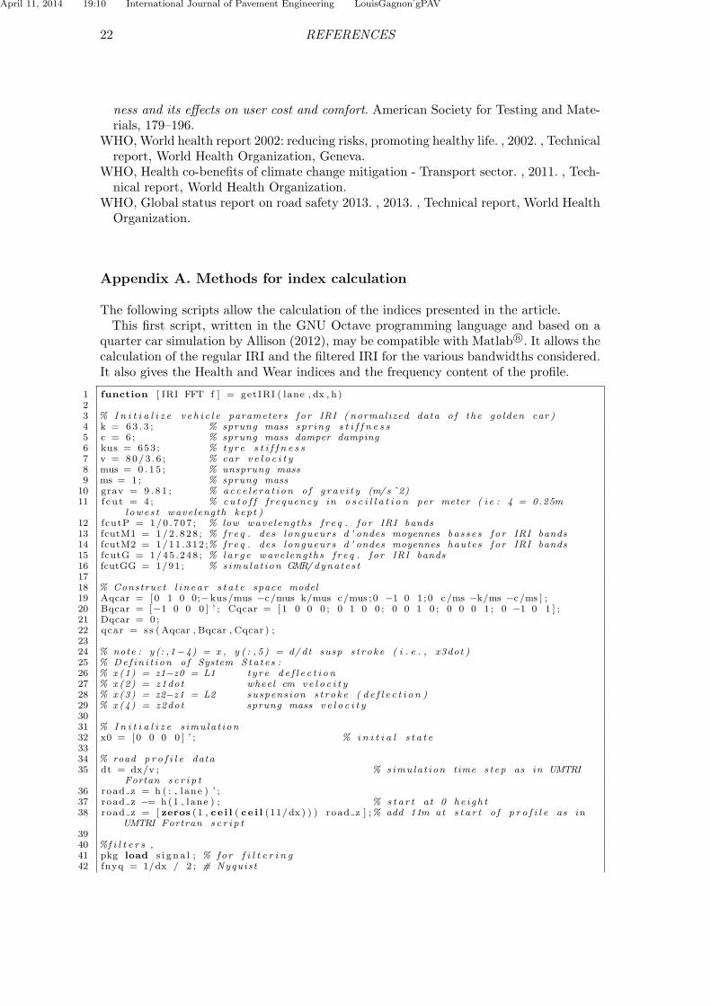
Appendix A. Methods for index calculation

The following scripts allow the calculation of the indices presented in the article.This first script, written in the GNU Octave programming language and based on a

quarter car simulation by Allison (2012), may be compatible with Matlab R⃝. It allows thecalculation of the regular IRI and the filtered IRI for the various bandwidths considered.It also gives the Health and Wear indices and the frequency content of the profile.

1 function [ IRI FFT f ] = getIRI ( lane , dx , h)23 % I n i t i a l i z e v e h i c l e parameters f o r IRI ( normalized data o f the go lden car )4 k = 63 . 3 ; % sprung mass spr ing s t i f f n e s s5 c = 6 ; % sprung mass damper damping6 kus = 653 ; % tyre s t i f f n e s s7 v = 80/3 . 6 ; % car v e l o c i t y8 mus = 0 . 1 5 ; % unsprung mass9 ms = 1 ; % sprung mass

10 grav = 9 . 8 1 ; % acce l e r a t i on o f g r a v i t y (m/s ˆ2)11 f cu t = 4 ; % cu t o f f f requency in o s c i l l a t i o n per meter ( i e : 4 = 0.25m

lowes t wave length kep t )12 fcutP = 1/0 . 707 ; % low wave lengths f r e q . f o r IRI bands13 fcutM1 = 1/2 . 828 ; % fr e q . des longueurs d ’ ondes moyennes bas se s f o r IRI bands14 fcutM2 = 1/11 . 312 ;% fr e q . des longueurs d ’ ondes moyennes hautes f o r IRI bands15 fcutG = 1/45 . 248 ; % la r g e wave lengths f r e q . f o r IRI bands16 fcutGG = 1/91 ; % simu la t ion GMR/dynates t1718 % Construct l i n e a r s t a t e space model19 Aqcar = [0 1 0 0;−kus/mus −c/mus k/mus c/mus ; 0 −1 0 1 ;0 c/ms −k/ms −c/ms ] ;20 Bqcar = [−1 0 0 0 ] ’ ; Cqcar = [1 0 0 0 ; 0 1 0 0 ; 0 0 1 0 ; 0 0 0 1 ; 0 −1 0 1 ] ;21 Dqcar = 0 ;22 qcar = s s (Aqcar , Bqcar , Cqcar ) ;2324 % note : y (: ,1−4) = x , y ( : , 5 ) = d/ dt susp s t r o k e ( i . e . , x3dot )25 % De f in i t i on o f System Sta t e s :26 % x (1) = z1−z0 = L1 ty re d e f l e c t i o n27 % x (2) = z1dot wheel cm v e l o c i t y28 % x (3) = z2−z1 = L2 suspension s t ro k e ( d e f l e c t i o n )29 % x (4) = z2dot sprung mass v e l o c i t y3031 % I n i t i a l i z e s imu la t ion32 x0 = [0 0 0 0 ] ’ ; % i n i t i a l s t a t e3334 % road p r o f i l e data35 dt = dx/v ; % simu la t ion time s t ep as in UMTRI

Fortan s c r i p t36 road z = h ( : , l ane ) ’ ;37 road z −= h(1 , lane ) ; % s t a r t at 0 he i gh t38 road z = [ zeros (1 , ce i l ( ce i l (11/dx ) ) ) road z ] ;% add 11m at s t a r t o f p r o f i l e as in

UMTRI Fortran s c r i p t3940 %f i l t e r s ,41 pkg load s i g n a l ; % for f i l t e r i n g42 fnyq = 1/dx / 2 ; # Nyquist


REFERENCES 23

43 road z ( 2 , : ) = road z ( 1 , : ) ;44 [ b f i l , a f i l ] = butte r (3 , [ fcutM1/ fnyq , fcutP/ fnyq ] ) ;45 road z ( 3 , : ) = f i l t f i l t ( b f i l , a f i l , road z ( 1 , : ) ) ;46 [ b f i l , a f i l ] = butte r (3 , [ fcutM2/ fnyq , fcutM1/ fnyq ] ) ;47 road z ( 4 , : ) = f i l t f i l t ( b f i l , a f i l , road z ( 1 , : ) ) ;48 [ b f i l , a f i l ] = butte r (3 , [ fcutG/ fnyq , fcutM2/ fnyq ] ) ;49 road z ( 5 , : ) = f i l t f i l t ( b f i l , a f i l , road z ( 1 , : ) ) ;50 [ b f i l , a f i l ] = butte r (3 , f cu t / fnyq ) ; % tyre f i l t e r se tup (250mm) , app l i ed i n s i d e

next loop51 %, f i l t e r s5253 road x = [ 0 : dx : ( s ize ( road z ( 1 , : ) ) (2 )−1)∗dx ] ; %using re f e r ence p r o f i l e l en g t h as

v a l i d f o r a l l f i l t e r e d p r o f i l e s54 tmax = road x (end) /v ; % simula t ion time l eng t h55 dt2 = dx/v ; % time s t ep f o r input data56 t = 0 : dt : tmax ; x = v∗ t ; % time/ space s t e p s to record

output5758 for waveCnt = 2 : 1 : 55960 road z (waveCnt , : ) = f i l t f i l t ( b f i l , a f i l , road z (waveCnt , : ) ) ;61 z0dot = [0 d i f f ( road z (waveCnt , : ) ) /dt2 ] ; % road p r o f i l e

v e l o c i t y62 u = interp1 ( road x , z0dot , x , ’ ∗ l i n e a r ’ , ’ extrap ’ ) ; % prepare s imu la t ion

input63 % Simulate quar ter car model ,64 y = ls im ( qcar , u , t , x0 ) ;65 deltamaxf = max(abs ( y ( : , 1 ) ) ) ; % max x3 ampl i tude66 z2dotdot = [0 d i f f ( y ( : , 4 ) ) ’/ dt2 ] ; % sprung mass a c c e l e r a t i on67 % ge t IRI ,68 IRI (waveCnt ) = sum(abs ( d i f f ( y ( : , 3 ) ) ) ) / ( ( x (end)−11)/1000) ;69 endfor7071 i f (1 ) % enab le to a c t i v a t e LRI (measures suspended mass a c c e l e r a t i on s as i f i t

were a sea t v i b r a t i on fo r hea l t h i nd i c a t i on s )72 waveCnt = 1 ; % using u n f i l t e r e d road fo r t h i s type o f e va l ua t i on73 z0dot = [0 d i f f ( road z (waveCnt , : ) ) /dt2 ] ; % road p r o f i l e

v e l o c i t y74 u = interp1 ( road x , z0dot , x , ’ ∗ l i n e a r ’ , ’ extrap ’ ) ; % prepare s imu la t ion

input75 % Simulate quar ter car model ,76 y = ls im ( qcar , u , t , x0 ) ;77 deltamaxf = max(abs ( y ( : , 1 ) ) ) ; % max x3 ampl i tude78 z2dotdot = [0 d i f f ( y ( : , 4 ) ) ’/ dt2 ] ; % sprung mass a c c e l e r a t i on79 % w k f r e q we igh t ing (ISO−2631−1) ,80 f1 = 0 . 4 ; w1 = 2∗pi∗ f 1 ;81 f2 = 100 ; w2 = 2∗pi∗ f 2 ;82 f3 = 12 . 5 ; w3 = 2∗pi∗ f 3 ;83 f4 = 12 . 5 ; w4 = 2∗pi∗ f 4 ;84 Q4 = 0 . 6 3 ;85 f5 = 2 . 3 7 ; w5 = 2∗pi∗ f 5 ;86 Q5 = 0 . 9 1 ;87 f6 = 3 . 3 5 ; w6 = 2∗pi∗ f 6 ;88 Q6 = 0 . 9 1 ;8990 Hh k = t f ( [ 1 0 0 ] , [ 1 sqrt (2 ) ∗w1 w1ˆ2 ] ) ; % Hh ( high pass )91 Hl k = t f ( [ 0 0 w2ˆ 2 ] , [ 1 sqrt (2 ) ∗w2 w2ˆ2 ] ) ; % Hl ( low pass )92 Ht k = t f ( [ 0 w4ˆ2/w3 w4ˆ 2 ] , [ 1 w4/Q4 w4ˆ2 ] ) ; % Ht ( acce l−v e l t r a n s i t i o n )93 Hs k = t f ( [ 1 /w5ˆ2 1/(Q5∗w5) 1 ] . ∗ ( w5/w6) ˆ2 , [ 1/w6ˆ2 1/(Q6∗w6) 1 ] ) ; % Hs (

upward s t ep )9495 Zseat = z2dotdot ; % t h i s i s not r e l a t e d to sea t but ra ther to sprung

mass96 Ts=dt ;97 Hh = Hh k ; Hl = Hl k ; Ht = Ht k ; Hs = Hs k ;98 [num, den ] = t fda ta (Hl , ’ v ’ ) ; [ B,A] = b i l i n e a r (num, den , Ts ) ; Zseat wk = f i l t e r

(B, A, Zseat ) ; [ num, den ] = t fda ta (Hh, ’ v ’ ) ; [ B,A] = b i l i n e a r (num, den , Ts ); Zseat wk = f i l t e r (B, A, Zseat wk ) ; [ num, den ] = t fda ta (Ht , ’ v ’ ) ; [ B,A] =b i l i n e a r (num, den , Ts ) ; Zseat wk = f i l t e r (B, A, Zseat wk ) ; [ num, den ] =

t fda ta (Hs , ’ v ’ ) ;99 a3 we = ( sum( Zseat wk .ˆ2 ) / length ( Zseat wk ) ) ˆ 0 . 5 ; %RMS


24 REFERENCES

100 a3 c r = max(abs ( Zseat wk ) ) / a3 we ; %cre s t101 a3 wf = ( sum( Zseat wk .ˆ4 ) / length ( Zseat wk ) ) ˆ 0 . 2 5 ; % 4 th power102 i f ( a3 c r > 9)103 IRI (waveCnt ) = a3 wf ;104 else105 IRI (waveCnt ) = a3 we ;106 endif107108 i f (2 )109 waveCnt = 6 ; % ra in f l ow count ing on suspension fo r ce110 r f s u s p en s i o n = ra in f l ow ( Zseat , t ) ;111 Dmg susp = sum( ( 2 . ∗ r f s u s p en s i o n ( 1 , : ) ) . ˆ 3 . ∗ r f s u s p en s i o n ( 3 , : ) ) ;112 IRI (waveCnt ) = Dmg susp ;113 endif114 endif115116 i f (3 ) % ca l c u l a t e f f t o f road117 L = s ize ( road z ) (2 ) ;118 NFFT = 2ˆnextpow2(L) ;119 Y = f f t ( road z ( 1 , : )−mean( road z ( 1 , : ) ) ,NFFT, 2 ) /L ; % al so s e t t i n g

mean to zero to avoid zero−f r eqency con t r i bu t i on o f s i g n a l120 f = 0 ;121 FFT = 2∗abs (Y( 1 :NFFT/2+1) ) ;122 endif123124 endfunction

A similar script allows the calculation of the Safety Index. One difference is that themain function accepts an additional parameter, BMP , which is the elongation of the tyrespring beyond which the accumulation of the index value is effected. This elongation wasset at 0.0175 m for the presented results. Thus, the differences from the previous scriptare that the function call is changed to,

1 function BM = getBoeingMod ( lane , dx , h ,BMP)

and the calculation of the index is done from the following lines of GNU Octave code,

1 i f (4 ) % measure l o s s e s o f contac t with the road2 BM = dx ∗ size ( find ( y ( : , 1 ) ’ >= BMP) ) (2 ) ; % tak ing the t o t a l d i s t ance

t r a v e l e d with tyre−road spr ing s t r eched above t h r e s ho l d ( peak ) WARNING: t h i s i s not an average , so w i l l vary between p r o f i l e s o f d i f f e r e n tl e n g t h s !

3 endif

Finally, to obtain the simple, two, and four point indices, a GNU Octave procedurealong the lines of what follows has been used to generate the average profiles prior tocalculating the indices,

1 [ IRI L FFT L f L ] = getIRI (1 , de l ta , h (numPre : ( s ize (h) (1 )−numPost ) , : ) ) ;2 [ IRI R FFT R f R ] = getIRI (2 , de l ta , h (numPre : ( s ize (h) (1 )−numPost ) , : ) ) ;3 IRI = ( IRI L+IRI R ) /2 ;4 FFT = (FFT L+FFT R) /2 ;5 hMean = (h ( : , 1 )+h ( : , 2 ) ) /2 ;6 [HRI HFFT Hf ] = getIRI (1 , de l ta , hMean(numPre : ( s ize (h) (1 )−numPost ) , 1 ) ) ;7 WB = 2 . 6 1 6 ; % ford focus 2002 whee lbase8 numAdded = ce i l (WB/ de l t a /2) ∗2 ; % added po in t s to p r o f i l e f o r f ront−rear mean9 hMeanF = ( ( [ hMean ; hMean(end) ∗ones (numAdded , 1 ) ] + [ hMean(1) ∗ones (numAdded , 1 ) ;

hMean ] ) /2) (numAdded/2 :end−numAdded/2) ;10 [ FRI FFFT Ff ] = getIRI (1 , de l ta , hMeanF(numPre : ( s ize (h) (1 )−numPost ) , 1 ) ) ;

Documents

RESEARCH ARTICLE An overview of various new road pro le ...louisgagnon.com/articleArchive/LouisGagnon_gPAV_finalSubmission.pdf · A steering algorithm similar to the moment-by-moment