Embed Size (px)
Citation preview
A Geometric Study of Single Gimbal Control Moment Gyros
— Singularity Problems and Steering Law —
Haruhisa Kurokawa
Mechanical Engineering Laboratory
Report of Mechanical Engineering Laboratory, No. 175, p.108, 1998.
––– i –––
In this research, a geometric study of singularity
characteristics and steering motion of single gimbal
Control Moment Gyros (CMGs) was carried out in orderto clarify singularity problems, to construct an effective
steering law, and to evaluate this law’s performance.
Passability, as defined by differential geometryclarified whether continuous steering motion is possible
in the neighborhood of a singular system state.
Topological study of general single gimbal CMGsclarified conditions for continuous steering motion over
a wider range of angular momentum space. It was shown
that there are angular momentum vector trajectories suchthat corresponding gimbal angles cannot be continuous.
If the command torque, as a function of time, results in
such a trajectory in the angular momentum space, anysteering law neither can follow the command exactly
nor can be effective.
A more detailed study of the symmetric pyramid type
of single gimbal CMGs clarified a more serious problem
of continuous steering, that is, no steering law can follow
all command sequences inside a certain region of theangular momentum space if the command is given in
real time. Based on this result, a candidate steering law
effective for rather small space was proposed and verifiednot only analytically, but also using ground experiments
which simulated attitude control in space.
Similar evaluation of other steering laws andcomparison of various system configurations in terms
of the allowed angular momentum region and the
system’s weight indicated that the pyramid type singlegimbal CMG system with the proposed steering law is
one of the most effective candidate torquer for attitude
control, having such advantages as a simple mechanism,a simpler steering law, and a larger angular momentum
space.
A Geometric Study of
Single Gimbal Control Moment Gyros
— Singularity Problems and Steering Law —
by
Haruhisa Kurokawa
Abstract
Keywords Attitude control, Singularity, Momentum exchange device, Inverse kinematics, Steering law
––– ii –––
This research work is a result of projects conductedat the Mechanical Engineering Laboratory, Agency of
Industrial Technology and Science, Ministry of
International Trade and Industry, Japan. Related projectsare, “Development of Attitude Control Equipment
(FY1982–1987)“, “Attitude Control System for Large
Space Structures (FY1988–1993)”, and “High PrecisionPosition and Attitude Control in Space (FY1993–1997)”.
I wish to acknowledge my debt to many people. Prof.Nobuyuki Yajima of the Institute of Space and
Astronautical Science (ISAS) are earnestly thanked for
inspiring me with this theme, as well as for collaborationsduring his tenure as a division head of our laboratory. I
would extend thanks to the late Prof. Toru Tanabe,
formerly of the University of Tokyo for his guidance inthe culmination of this work into a dissertation. In
finishing this work, the following professors guided me,Assoc. Prof. Shinichi Nakasuka of the University Tokyo,
Prof. Hiroki Matsuo of ISAS, Prof. Shinji Suzuki, Prof.
Yoshihiko Nakamura, Assoc. Prof. Ken Sasaki of theUniversity of Tokyo.
Many discussions with Dr. Shigeru Kokaji of our
laboratory proved invaluable. He patiently listened tomy abstract explanation of geometry and provided
valuable suggestions. Furthermore, he assisted me by
soldering and checking circuits, and reviewed this paper June 7, 1997
Acknowledgments
from cover-to-cover, providing constructive criticism.I would also like to thank my colleague Akio Suzuki
who constructed most of the experimental apparatus, and
designed and installed controllers for the attitude control.Prof. Tsuneo Yoshikawa of Kyoto University helped
me when we started the project of attitude control by
CMGs. Discussions held with Dr. Nazareth Bedrossianand Dr. Joseph Paradiso of the Charles Stark Draper
Laboratory (CSDL) were invaluable. They gave me
valuable suggestions with various research papers in thisfield.
Dr. Mark Lee Ford as a visiting researcher of our
laboratory spent his precious hours for me to correctexpressions in English.
I would like to thank all the above people, other
colleagues sharing other research projects, and theMechanical Engineering Laboratory (MEL) and the
directors especially the Director General Dr. Kenichi
Matuno and the former Department Head Dr. KiyofumiMatsuda for allowing me to continue this research.
Finally, I thank my wife and daughters for their patience
particularly during some hectic months.
Haruhisa Kurokawa
––– iii –––
Contents
Abstract ............................................................................................................................................................ i
Acknowledgments ........................................................................................................................................... ii
Terms ........................................................................................................................................................... viii
Nomenclature ................................................................................................................................................. ix
List of Figures ................................................................................................................................................. x
List of Tables ............................................................................................................................................... xiii
Chapter 1 Introduction .............................................................................................. 1
1.1 Research Background ..................................................................................................................................... 1
1.2 Scope of Discussion ........................................................................................................................................ 3
1.3 Outline of this Thesis ...................................................................................................................................... 4
Chapter 2 Characteristics of Control Moment Gyro Systems ............................... 5
2.1 CMG Unit Type ............................................................................................................................................. 5
2.2 System Configuration .................................................................................................................................... 5
2.2.1 Single Gimbal CMGs ............................................................................................................................ 6
2.2.2 Two Dimensional System and Twin Type System ................................................................................ 7
2.2.3 Configuration of Double Gimbal CMGs............................................................................................... 7
2.3 Three Axis Attitude Control ........................................................................................................................... 7
2.3.1 Block Diagram ...................................................................................................................................... 8
2.3.2 CMG Steering Law ............................................................................................................................... 8
2.3.3 Momentum Management ...................................................................................................................... 8
2.3.4 Maneuver Command ............................................................................................................................. 8
2.3.5 Disturbance ........................................................................................................................................... 8
2.3.6 Angular Momentum Trajectory ............................................................................................................. 8
2.4 Comparison and Selection ............................................................................................................................. 9
2.4.1 Performance Index ................................................................................................................................ 9
2.4.2 Component Level Comparison ............................................................................................................. 9
2.4.3 System Level Comparison .................................................................................................................... 9
2.4.4 Work Space Size and Weight ................................................................................................................ 9
Chapter 3 General Formulation .............................................................................. 11
3.1 Angular Momentum and Torque ................................................................................................................... 11
3.2 Steering Law ................................................................................................................................................. 12
3.3 Singular Value Decomposition and I/O Ratio ............................................................................................... 12
3.4 Singularity ..................................................................................................................................................... 13
––– iv –––
3.5 Singularity Avoidance ................................................................................................................................... 13
3.5.1 Gradient Method ................................................................................................................................. 14
3.5.2 Steering in Proximity to a Singular State ............................................................................................. 14
Chapter 4 Singular Surface and Passability .......................................................... 15
4.1 Singular Surface ........................................................................................................................................... 15
4.1.1 Continuous Mapping ........................................................................................................................... 15
4.1.2 Envelope .............................................................................................................................................. 16
4.1.3 Visualization Method of the Surface ................................................................................................... 16
4.2 Differential Geometry .................................................................................................................................. 17
4.2.1 Tangent Space and Subspace............................................................................................................... 17
4.2.2 Gaussian Curvature ............................................................................................................................. 17
4.3 Passability .................................................................................................................................................... 18
4.3.1 Quadratic Form ................................................................................................................................... 18
4.3.2 Signature of Quadratic Form............................................................................................................... 19
4.3.3 Passability and Singularity Avoidance ................................................................................................ 19
4.3.4 Discrimination ..................................................................................................................................... 20
4.4 Internal Impassable Surface ......................................................................................................................... 21
4.4.1 Impassable Surface of an Independent Type System .......................................................................... 21
4.4.2 Impassable Surface of a Multiple Type System .................................................................................. 21
4.4.3 Minimum System ................................................................................................................................ 22
Chapter 5 Inverse Kinematics ................................................................................. 23
5.1 Manifold ....................................................................................................................................................... 23
5.2 Manifold Path .............................................................................................................................................. 24
5.3 Domain and Equivalence Class ................................................................................................................... 24
5.4 Terminal Class and Domain Type ................................................................................................................ 25
5.5 Class Connection ......................................................................................................................................... 25
5.5.1 Type 2 Domain .................................................................................................................................... 25
5.5.2 Type 1 Domain .................................................................................................................................... 26
5.5.3 Class Connection Rules....................................................................................................................... 27
5.5.4 Continuous Steering over Domains .................................................................................................... 28
5.5.5 Manifold Selection .............................................................................................................................. 28
5.5.6 Discussion of the Critical Point ........................................................................................................... 29
5.6 Topological Problem ..................................................................................................................................... 29
Chapter 6 Pyramid Type CMG System ................................................................... 31
6.1 System Definition ........................................................................................................................................ 31
6.2 Symmetry ..................................................................................................................................................... 31
6.3 Singular Manifold for the H Origin ............................................................................................................. 33
––– v –––
6.4 Singular Surface Geometry .......................................................................................................................... 35
Chapter 7 Global Problem, Steering Law Exactness and Proposal ................... 41
7.1 Global Problem ............................................................................................................................................ 41
7.1.1 Control Along the z Axis ..................................................................................................................... 41
7.1.2 Global problem.................................................................................................................................... 45
7.1.3 Details of the Problem ......................................................................................................................... 45
7.1.4 Possible Solutions ............................................................................................................................... 47
7.2 Steering Law with Error .............................................................................................................................. 47
7.2.1 Geometrical Meaning .......................................................................................................................... 47
7.2.2 Exactness of Control ........................................................................................................................... 48
7.3 Path Planning ............................................................................................................................................... 49
7.4 Preferred Gimbal Angle ............................................................................................................................... 49
7.5 Exact Steering Law ...................................................................................................................................... 51
7.5.1 Workspace Restriction ......................................................................................................................... 51
7.5.2 Repeatability and Unique Inversion .................................................................................................... 51
7.5.3 Constrained Control ............................................................................................................................ 52
7.5.4 Reduced Workspace ............................................................................................................................ 52
7.5.5 Characteristics of Constrained Control ............................................................................................... 54
Chapter 8 Ground Experiments .............................................................................. 57
8.1 Attitude Control ........................................................................................................................................... 57
8.1.1 Dynamics ............................................................................................................................................. 57
8.1.2 Exact Linearization ............................................................................................................................. 57
8.1.3 Control Method ................................................................................................................................... 58
8.2 Experimental Facility and Procedure ........................................................................................................... 58
8.2.1 Facility ................................................................................................................................................. 58
8.2.2 Design of Control Command Sequence .............................................................................................. 59
8.2.3 Experimental Procedure ...................................................................................................................... 59
8.3 Experimental Results ................................................................................................................................... 60
8.3.1 Attitude Keeping under Constant Disturbance .................................................................................... 60
8.3.2 Rotation About the z Axis ................................................................................................................... 64
8.3.3 Maneuver after Momentum Accumulation ......................................................................................... 67
8.3.4 Mode Selection and Switching............................................................................................................. 69
8.4 Summary of Experiments ............................................................................................................................ 69
Chapter 9 Evaluation ............................................................................................... 71
9.1 Conditions for Comparison .......................................................................................................................... 71
9.2 Spherical Workspace .................................................................................................................................... 71
9.3 Evaluation by Weight ................................................................................................................................... 72
––– vi –––
9.4 Ellipsoidal Workspace ................................................................................................................................. 73
9.5 Summary of Evaluation ................................................................................................................................ 75
Chapter 10 Conclusions .......................................................................................... 77
Appendix A Double Gimbal CMG System .............................................................. 79
A.1 General Formulation ................................................................................................................................... 79
A.2 Singularity ................................................................................................................................................... 79
A.3 Steering Law and Null Motion ................................................................................................................... 80
A.4 Passability ................................................................................................................................................... 80
A.4.1 Two Unit System ................................................................................................................................ 80
A.4.2 Three Unit System .............................................................................................................................. 81
A.5 Workspace ................................................................................................................................................... 81
Appendix B Proofs of Theories ............................................................................... 83
B.1 Basis of Tangent Spaces .............................................................................................................................. 83
B.2 Gaussian Curvature ..................................................................................................................................... 83
B.3 Inverse Mapping Theory ............................................................................................................................. 84
B.4 Impassable condition for two negative signs .............................................................................................. 85
Appendix C Internal Impassability of Multiple Type Systems .............................. 87
C.1 Roof Type System M(2, 2) .......................................................................................................................... 87
C.1.1 Evaluation of Singular Surface (2) ..................................................................................................... 87
C.1.2 Evaluation of Singular Surface (3) ..................................................................................................... 87
C.1.3 Evaluation of Singular Surface (5) ..................................................................................................... 88
C.1.4 Evaluation of Singular Surface (7) ..................................................................................................... 88
C.1.5 Conclusion .......................................................................................................................................... 88
C.2 M(3, 2): M(2, 2)+1 ...................................................................................................................................... 88
C.2.1 Condition (3) of M(2,2) ...................................................................................................................... 88
C.2.2 Condition (5) of M(2,2) ...................................................................................................................... 89
C.3 M(3, 3): M(2, 2)+2 ...................................................................................................................................... 89
C.4 M(2, 2, 1): M(2, 2)+1 .................................................................................................................................. 89
C.5 M(2, 2, 2): M(2, 2)+2 .................................................................................................................................. 89
C.6 Minimum System ........................................................................................................................................ 89
Appendix D Six and Five Unit Systems .................................................................. 91
D.1 Symmetric Six Unit System S(6) ................................................................................................................. 91
D.1.1 System Definition ................................................................................................................................ 91
––– vii –––
D.1.2 Fault Management ............................................................................................................................... 91
D.1.3 Four out of Six Control ....................................................................................................................... 92
D.2 Five Unit Skew System ................................................................................................................................ 92
Appendix E Specification of Experimental Apparatus and Experimental Procedure
. ................................................................................................... 95
E.1 Experimental Apparatus .............................................................................................................................. 95
E.2 Specifications .............................................................................................................................................. 97
E.3 Attitude Control System .............................................................................................................................. 97
E.4 Steering Law Implementation ..................................................................................................................... 99
E.5 Code Size and Calculation Time ................................................................................................................. 99
E.6 Parameter Estimation .................................................................................................................................. 99
Appendix F General kinematics ............................................................................ 101
F.1 Analogy with a Spatial Link Mechanism ................................................................................................... 101
F.2 Spatial Link Mechanism Kinematics ......................................................................................................... 101
F.3 Singularity .................................................................................................................................................. 102
F.4 Passability .................................................................................................................................................. 102
References ............................................................................................................... 105
––– viii –––
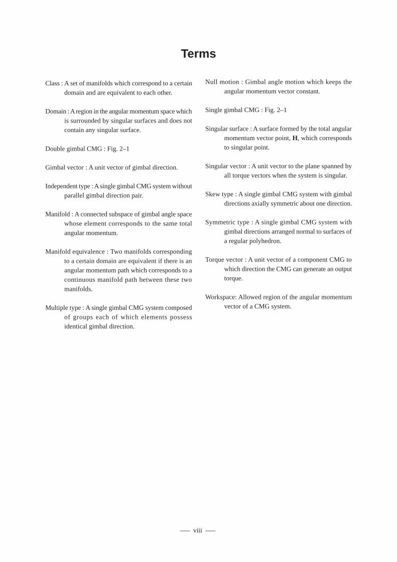
Terms
Class : A set of manifolds which correspond to a certain
domain and are equivalent to each other.
Domain : A region in the angular momentum space which
is surrounded by singular surfaces and does notcontain any singular surface.
Double gimbal CMG : Fig. 2–1
Gimbal vector : A unit vector of gimbal direction.
Independent type : A single gimbal CMG system without
parallel gimbal direction pair.
Manifold : A connected subspace of gimbal angle space
whose element corresponds to the same total
angular momentum.
Manifold equivalence : Two manifolds corresponding
to a certain domain are equivalent if there is anangular momentum path which corresponds to a
continuous manifold path between these two
manifolds.
Multiple type : A single gimbal CMG system composed
of groups each of which elements possessidentical gimbal direction.
Null motion : Gimbal angle motion which keeps the
angular momentum vector constant.
Single gimbal CMG : Fig. 2–1
Singular surface : A surface formed by the total angularmomentum vector point, H, which corresponds
to singular point.
Singular vector : A unit vector to the plane spanned by
all torque vectors when the system is singular.
Skew type : A single gimbal CMG system with gimbal
directions axially symmetric about one direction.
Symmetric type : A single gimbal CMG system with
gimbal directions arranged normal to surfaces of
a regular polyhedron.
Torque vector : A unit vector of a component CMG to
which direction the CMG can generate an outputtorque.
Workspace: Allowed region of the angular momentumvector of a CMG system.
––– ix –––
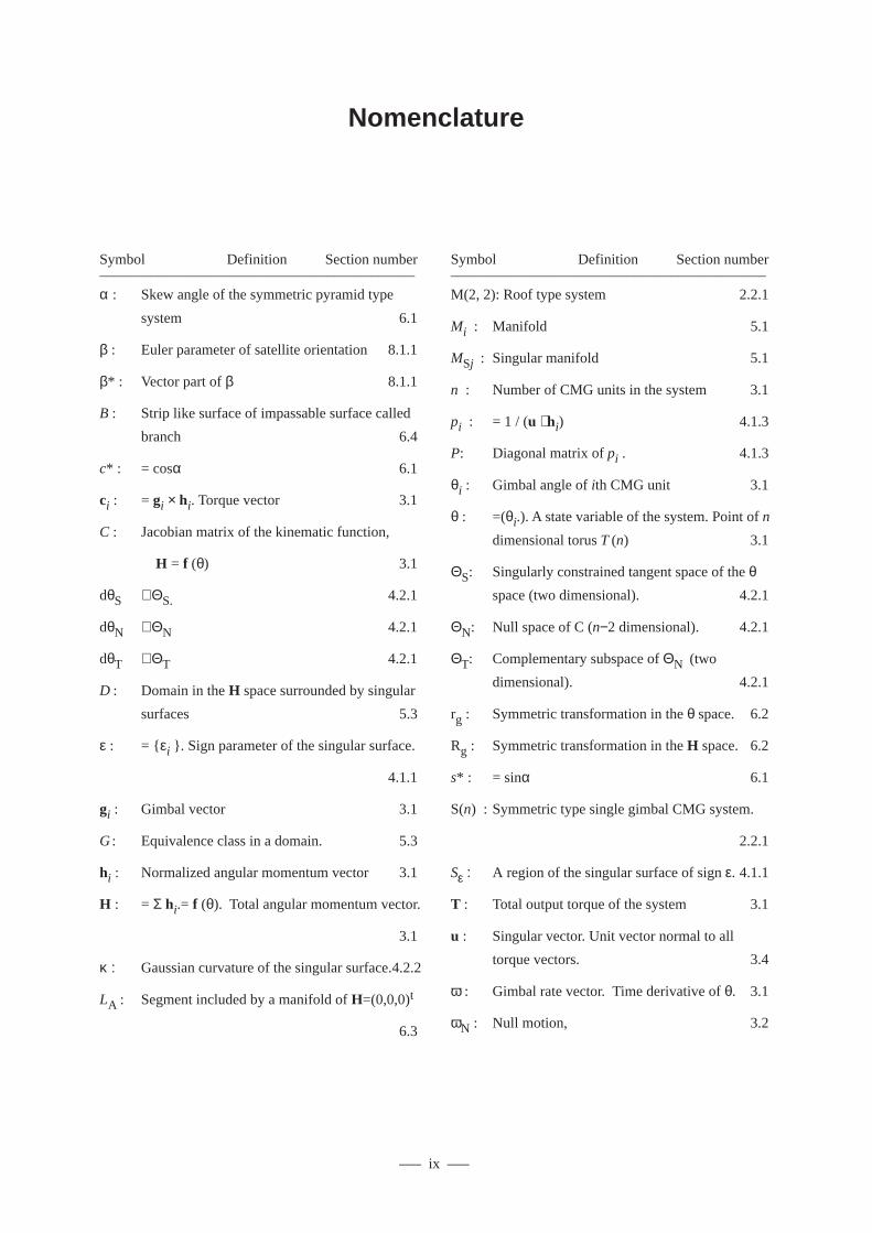
Symbol Definition Section number–––––––––––––––––––––––––––––––––––––––––––α : Skew angle of the symmetric pyramid type
system 6.1
β : Euler parameter of satellite orientation 8.1.1
β* : Vector part of β 8.1.1
B : Strip like surface of impassable surface called
branch 6.4
c* : = cosα 6.1
ci : = gi × hi. Torque vector 3.1
C : Jacobian matrix of the kinematic function,
H = f (θ) 3.1
dθS ∈ΘS. 4.2.1
dθN ∈ΘN 4.2.1
dθT ∈ΘT 4.2.1
D : Domain in the H space surrounded by singular
surfaces 5.3
ε : = {εi }. Sign parameter of the singular surface.
4.1.1
gi : Gimbal vector 3.1
G : Equivalence class in a domain. 5.3
hi : Normalized angular momentum vector 3.1
H : = Σ hi.= f (θ). Total angular momentum vector.
3.1
κ : Gaussian curvature of the singular surface.4.2.2
LA : Segment included by a manifold of H=(0,0,0)t
6.3
Nomenclature
Symbol Definition Section number–––––––––––––––––––––––––––––––––––––––––––M(2, 2): Roof type system 2.2.1
Mi : Manifold 5.1
MSj : Singular manifold 5.1
n : Number of CMG units in the system 3.1
pi : = 1 / (u ⋅ hi) 4.1.3
P: Diagonal matrix of pi . 4.1.3
θi : Gimbal angle of ith CMG unit 3.1
θ : =(θi.). A state variable of the system. Point of n
dimensional torus T (n) 3.1
ΘS: Singularly constrained tangent space of the θspace (two dimensional). 4.2.1
ΘN: Null space of C (n−2 dimensional). 4.2.1
ΘT: Complementary subspace of ΘN (two
dimensional). 4.2.1
rg : Symmetric transformation in the θ space. 6.2
Rg : Symmetric transformation in the H space. 6.2
s* : = sinα 6.1
S(n) : Symmetric type single gimbal CMG system.
2.2.1
Sε : A region of the singular surface of sign ε. 4.1.1
T : Total output torque of the system 3.1
u : Singular vector. Unit vector normal to all
torque vectors. 3.4
ω : Gimbal rate vector. Time derivative of θ. 3.1
ωN : Null motion, 3.2
––– x –––
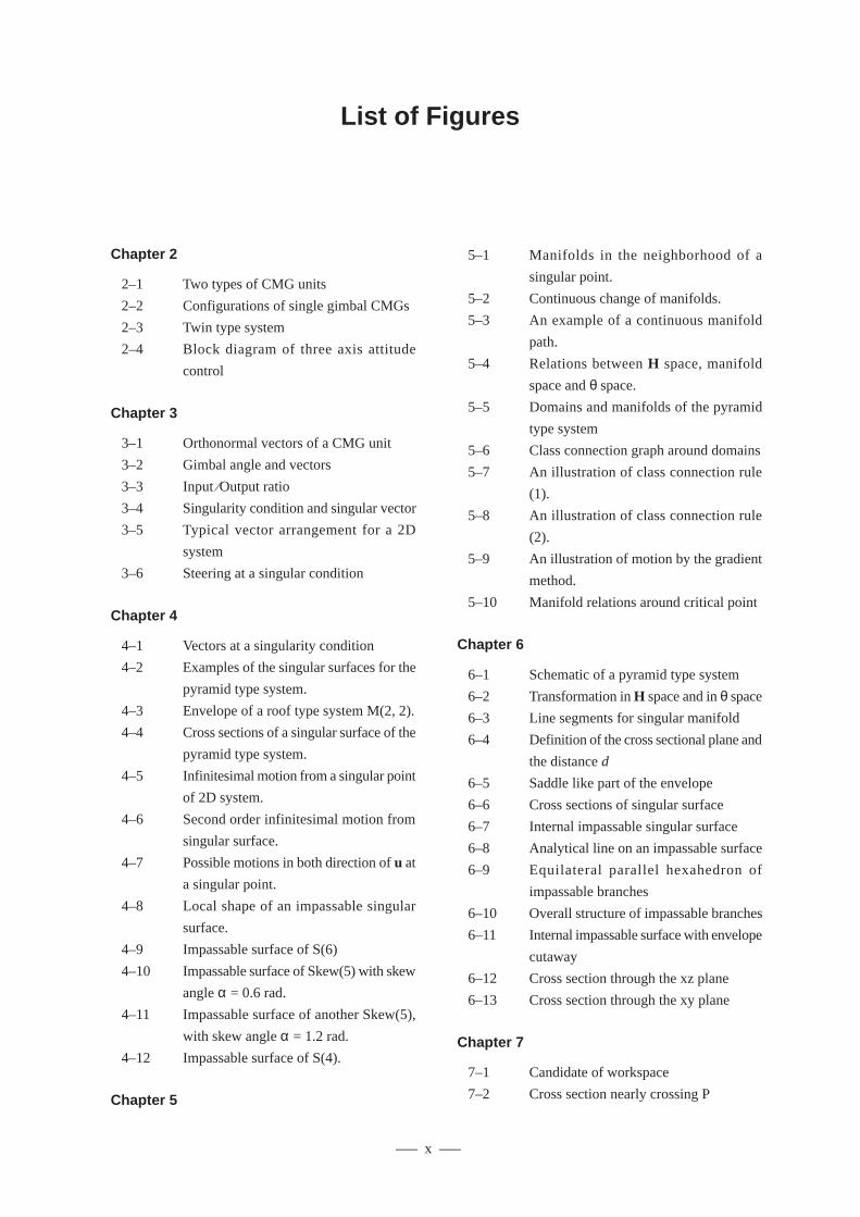
Chapter 2
2–1 Two types of CMG units
2–2 Configurations of single gimbal CMGs
2–3 Twin type system
2–4 Block diagram of three axis attitude
control
Chapter 3
3–1 Orthonormal vectors of a CMG unit
3–2 Gimbal angle and vectors
3–3 Input ⁄Output ratio
3–4 Singularity condition and singular vector
3–5 Typical vector arrangement for a 2D
system
3–6 Steering at a singular condition
Chapter 4
4–1 Vectors at a singularity condition
4–2 Examples of the singular surfaces for the
pyramid type system.
4–3 Envelope of a roof type system M(2, 2).
4–4 Cross sections of a singular surface of the
pyramid type system.
4–5 Infinitesimal motion from a singular point
of 2D system.
4–6 Second order infinitesimal motion from
singular surface.
4–7 Possible motions in both direction of u at
a singular point.
4–8 Local shape of an impassable singular
surface.
4–9 Impassable surface of S(6)
4–10 Impassable surface of Skew(5) with skew
angle α = 0.6 rad.
4–11 Impassable surface of another Skew(5),
with skew angle α = 1.2 rad.
4–12 Impassable surface of S(4).
Chapter 5
5–1 Manifolds in the neighborhood of a
singular point.
5–2 Continuous change of manifolds.
5–3 An example of a continuous manifold
path.
5–4 Relations between H space, manifold
space and θ space.
5–5 Domains and manifolds of the pyramid
type system
5–6 Class connection graph around domains
5–7 An illustration of class connection rule
(1).
5–8 An illustration of class connection rule
(2).
5–9 An illustration of motion by the gradient
method.
5–10 Manifold relations around critical point
Chapter 6
6–1 Schematic of a pyramid type system
6–2 Transformation in H space and in θ space
6–3 Line segments for singular manifold
6–4 Definition of the cross sectional plane and
the distance d
6–5 Saddle like part of the envelope
6–6 Cross sections of singular surface
6–7 Internal impassable singular surface
6–8 Analytical line on an impassable surface
6–9 Equilateral parallel hexahedron of
impassable branches
6–10 Overall structure of impassable branches
6–11 Internal impassable surface with envelope
cutaway
6–12 Cross section through the xz plane
6–13 Cross section through the xy plane
Chapter 7
7–1 Candidate of workspace
7–2 Cross section nearly crossing P
List of Figures
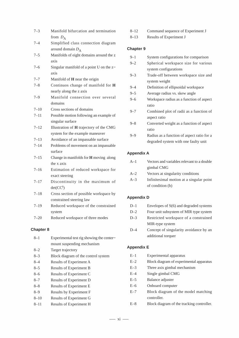
––– xi –––
7–3 Manifold bifurcation and termination
from DA 7–4 Simplified class connection diagram
around domain DA 7–5 Manifolds of eight domains around the z
axis
7–6 Singular manifold of a point U on the z−axis
7–7 Manifold of H near the origin
7–8 Continuos change of manifold for H
nearly along the z axis
7–9 Manifold connection over several
domains
7–10 Cross sections of domains
7–11 Possible motion following an example of
singular surface
7–12 Illustration of H trajectory of the CMG
system for the example maneuver
7–13 Avoidance of an impassable surface
7–14 Problems of movement on an impassable
surface
7–15 Change in manifolds for H moving along
the x axis
7–16 Estimation of reduced workspace for
exact steering
7–17 Discontinuity in the maximum of
det(CCt)
7–18 Cross section of possible workspace by
constrained steering law
7–19 Reduced workspace of the constrained
system
7–20 Reduced workspace of three modes
Chapter 8
8–1 Experimental test rig showing the center−mount suspending mechanism
8–2 Target trajectory
8–3 Block diagram of the control system
8–4 Results of Experiment A
8–5 Results of Experiment B
8–6 Results of Experiment C
8–7 Results of Experiment D
8–8 Results of Experiment E
8–9 Results by Experiment F
8–10 Results of Experiment G
8–11 Results of Experiment H
8–12 Command sequence of Experiment J
8–13 Results of Experiment J
Chapter 9
9–1 System configurations for comparison
9–2 Spherical workspace size for various
system configurations
9–3 Trade-off between workspace size and
system weight
9–4 Definition of ellipsoidal workspace
9–5 Average radius vs. skew angle
9–6 Workspace radius as a function of aspect
ratio
9–7 Combined plot of radii as a function of
aspect ratio
9–8 Converted weight as a function of aspect
ratio
9–9 Radius as a function of aspect ratio for a
degraded system with one faulty unit
Appendix A
A–1 Vectors and variables relevant to a double
gimbal CMG
A–2 Vectors at singularity conditions
A–3 Infinitesimal motion at a singular point
of condition (b)
Appendix D
D–1 Envelopes of S(6) and degraded systems
D–2 Four unit subsystem of MIR type system
D–3 Restricted workspace of a constrained
MIR-type system
D–4 Concept of singularity avoidance by an
additional torquer
Appendix E
E–1 Experimental apparatus
E–2 Block diagram of experimental apparatus
E–3 Three axis gimbal mechanism
E–4 Single gimbal CMG
E–5 Balance adjuster
E–6 Onboard computer
E–7 Block diagram of the model matching
controller.
E–8 Block diagram of the tracking controller.

––– xii –––
E–9 Block diagram of the gradient method.
E–10 Block diagram of the constrained method.
Appendix F
F−1 Analogy to a parallel link mechanism
––– xiii –––
List of Tables
Chapter 2
2–1 Component Level Comparison
2–2 System Level Comparison
Chapter 6
6–1 Symmetric Transformations
6–2 Segment Transformation Rule
Chapter 8
8–1 Condition and Results of Experiments (1)
8–2 Condition and Results of Experiments (2)
Appendix E
E–1 Specification of experimental apparatus
E–2 Code size and calculation time of process
Appendix F
F–1 Similarity between CMGs and link
mechanism

––– xiv –––
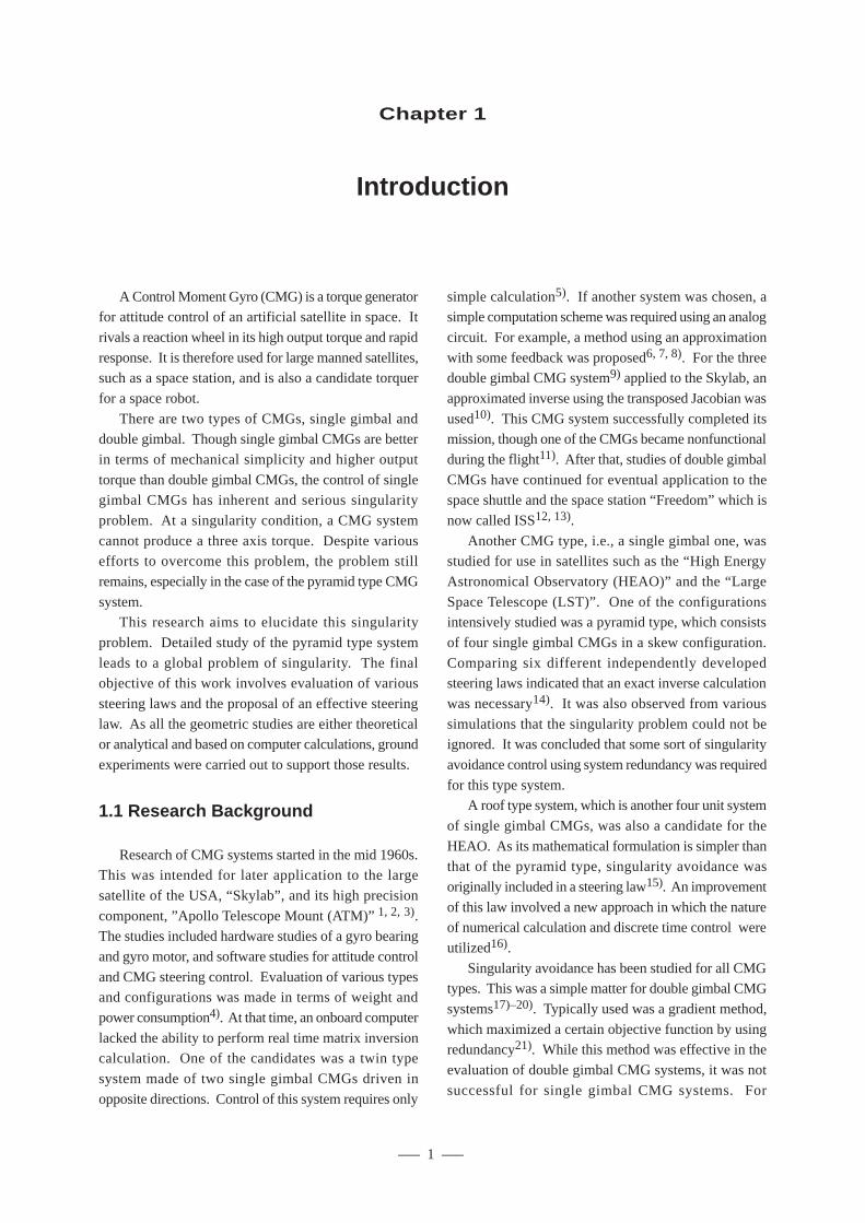
––– 1 –––
–– 2. Characteristics of Control Moment Gyro Systems ––
A Control Moment Gyro (CMG) is a torque generatorfor attitude control of an artificial satellite in space. It
rivals a reaction wheel in its high output torque and rapid
response. It is therefore used for large manned satellites,such as a space station, and is also a candidate torquer
for a space robot.
There are two types of CMGs, single gimbal anddouble gimbal. Though single gimbal CMGs are better
in terms of mechanical simplicity and higher output
torque than double gimbal CMGs, the control of singlegimbal CMGs has inherent and serious singularity
problem. At a singularity condition, a CMG system
cannot produce a three axis torque. Despite variousefforts to overcome this problem, the problem still
remains, especially in the case of the pyramid type CMG
system.This research aims to elucidate this singularity
problem. Detailed study of the pyramid type system
leads to a global problem of singularity. The finalobjective of this work involves evaluation of various
steering laws and the proposal of an effective steering
law. As all the geometric studies are either theoreticalor analytical and based on computer calculations, ground
experiments were carried out to support those results.
1.1 Research Background
Research of CMG systems started in the mid 1960s.This was intended for later application to the large
satellite of the USA, “Skylab”, and its high precision
component, ”Apollo Telescope Mount (ATM)” 1, 2, 3).The studies included hardware studies of a gyro bearing
and gyro motor, and software studies for attitude control
and CMG steering control. Evaluation of various typesand configurations was made in terms of weight and
power consumption4). At that time, an onboard computer
lacked the ability to perform real time matrix inversioncalculation. One of the candidates was a twin type
system made of two single gimbal CMGs driven in
opposite directions. Control of this system requires only
simple calculation5). If another system was chosen, asimple computation scheme was required using an analog
circuit. For example, a method using an approximation
with some feedback was proposed6, 7, 8). For the threedouble gimbal CMG system9) applied to the Skylab, an
approximated inverse using the transposed Jacobian was
used10). This CMG system successfully completed itsmission, though one of the CMGs became nonfunctional
during the flight11). After that, studies of double gimbal
CMGs have continued for eventual application to thespace shuttle and the space station “Freedom” which is
now called ISS12, 13).
Another CMG type, i.e., a single gimbal one, wasstudied for use in satellites such as the “High Energy
Astronomical Observatory (HEAO)” and the “Large
Space Telescope (LST)”. One of the configurationsintensively studied was a pyramid type, which consists
of four single gimbal CMGs in a skew configuration.
Comparing six different independently developedsteering laws indicated that an exact inverse calculation
was necessary14). It was also observed from various
simulations that the singularity problem could not beignored. It was concluded that some sort of singularity
avoidance control using system redundancy was required
for this type system.A roof type system, which is another four unit system
of single gimbal CMGs, was also a candidate for the
HEAO. As its mathematical formulation is simpler thanthat of the pyramid type, singularity avoidance was
originally included in a steering law15). An improvement
of this law involved a new approach in which the natureof numerical calculation and discrete time control were
utilized16).
Singularity avoidance has been studied for all CMGtypes. This was a simple matter for double gimbal CMG
systems17)–20). Typically used was a gradient method,
which maximized a certain objective function by usingredundancy21). While this method was effective in the
evaluation of double gimbal CMG systems, it was not
successful for single gimbal CMG systems. For
Chapter 1
Introduction
––– 2 –––
–– Technical Report of Mechanical Engineering Laboratory No.175 ––
example, optimization of a redundant variable resulted
in discontinuity16) or an optimized value became
singular15) in the case of a roof type system. In the caseof a pyramid type system, various problems were found
in computer simulations even when a gradient method
was used.Margulies was the first to formulate a theory of
singularity and control22). His paper included geometric
theory of a singular surface, a generalized solution ofthe output equation and null motion, and the possibility
of singularity avoidance for a general single gimbal CMG
system. Also, some problems of the gradient methodwere pointed out using an example of a two dimensional
system.
Works by the Russian researcher, Tokar, werepublished in the same year, and included a description
of the singular surface shape23), the size of the
workspace24) and some considerations of the gimballimits25). In his next paper26), passability of a singular
surface was introduced. It was made clear that a system
such as a pyramid type has an ‘impassable’ surface insideits workspace. Moreover, the problems of steering near
such an impassable surface were described. In spite of
those important results, his work was not widelyreceived, because the original papers were published in
Russian. Even though an English translation appeared,
several terms were used for a CMG, such as “gyroforce”,“gyro stabilizer” and “gyrodyne”. His conclusion was
that a system with no less that six units would provide
an adequately sized workspace including no impassablesurfaces. After this work, a six unit symmetric system
was designed for the Russian space station “MIR”27).
Some years later after Tokar’s studies, Kurokawaformulated passability again28) in terms of the geometric
theory given by Margulies. Most of these results
coincided with Tokar’s work. In addition, the existenceof impassability in the roof type system was clarified29)
and a discrimination method using the surface curvature
was presented30,31,32,33). In the last paper, the theorywas expanded to a general system including a double
gimbal CMG system. It was made clear that multiple
systems of no less than six units do not have any internalimpassable surface, while any system of less that six
units must have such a surface. Various configurations,
even containing faulty units, were compared with regardto their workspace size as an extension of Tokar’s work.
Along with these theoretical and general research
works, intensive efforts continued to find an effectivesteering law regarding the passability problem as a local
problem. Most of these dealt with the pyramid type
system. The reason this type was selected was because
a six unit system was considered too large and too
complicated. Many proposals suggested a type ofgradient method34, 35, 36). The method utilized for the
four unit subsystem of the “MIR” was also of this
kind27). Another method used global optimization28),and nearly all methods showed some problems in
computer simulations.
Passability is defined locally and its problem reportedfirst was a kind of local problem28). Later, Bauer showed
difficulty in steering as a global problem37). He found
two different command sequences, both of which couldnot be realized by the same steering method. After this,
Vadali proposed a method to overcome this problem
using a preferred state38). Finally, the problem by Bauerwas formulated exactly, stating that no steering law can
follow an arbitrary command sequence inside certain
wide region of the workspace39). Under this limitation,an effective method was proposed.
The research described above dealt with exact
control, but other research has also been carried out. Oneresearch effort permitted an error in the output if required.
Generalized inverse Jacobian22) minimizes the error.
Extension of this method, called the SR inverse method,was first proposed for control of a manipulator and later
applied to CMG control40,41). Another research type
dealt with path planning. If the command sequence inthe near future is given, steering can be planned
beforehand which realizes not only singularity avoidance
but also some degree of optimization42, 43, 44). In oneof the research papers43), some paths were chosen by
Kurokawa in consideration of impassable surfaces. Since
all these tended to take a heuristic approach, evaluationwas made by computer simulation considering attitude
control of a given satellite.
More realistic studies have also been made whichdealt with attitude control using a CMG system,
considering disturbance and other torquers. The largest
problem may be a precision control using a CMG system.Since a CMG system can generate a large output torque
and its output resolution is critical for precision control,
various analyses and simulations have shown thatpointing control by a CMG system can result in a limit
cycle because of friction in gimbal motion45, 46, 47). In
spite of efforts such as improvement of motor control48)
and torque cancellation by additional reaction wheels49),
the problem of precision control has not been overcome.
For application to the space station, another studies werecarried out such as an effective combination of a CMG
and RCS50) and integration of CMGs and power
––– 3 –––
–– 2. Characteristics of Control Moment Gyro Systems ––
storage51). In order to evaluate its attitude control
performance, not only numerical simulations, but also
some experiments using real mechanisms have beenmade, such as a platform supported by a spherical air
bearing44, 52). The author also developed ground test
equipment using normal ball bearings53) and attemptedrobust attitude control using a CMG system54,55).
The motion of a CMG system with regard to the
motion of the angular momentum vector is similar tothe motion of a link mechanism22). Analysis of the
motion and control of such a mechanism has been widely
studied. Those results were, therefore, used for CMGcontrol40, 41). On the other hand, some researchers first
studied CMG control and then applied their results to a
robot control56, 57, 58). In spite of various researches inrobot kinematics59, 60, 61), generalized theory for
singularity and inverse kinematics has not been
formulated yet.
1.2 Scope of Discussion
This research effort deals with the following subjects:
(1) General formulation of an arbitrarily configured
CMG system, especially of single gimbal CMGs.(2) Geometric study of the singularity problem of a
general single gimbal CMG system.
(3) Problem of exact and real-time steering of thepyramid type CMG system.
(4) Proposal and evaluation of steering laws for the
pyramid type CMG system.(5) Evaluation of various CMG systems.
The main purposes of this work are to clarify the
singularity problems, to construct an exact and strictlyreal-time steering law, and to specify and evaluate its
performance. Among all, singularity problems are the
most important relating to the others. A singularity candegrade a CMG system, even causing the system to loose
control, and this situation might be fatal for an artificial
satellite. Therefore, a CMG system must haveredundancy and it must be controlled to avoid
singularities by using an appropriate steering law.
Problems include whether such singularity avoidance isglobally possible and which steering law can realize such
control. Even if a steering law cannot avoid all the
singularities, the system’s working range of the angularmomentum must be specified in which singularity
avoidance is strictly guaranteed because such
specification is necessary for designing the total attitudecontrol system. Thus, this work deals with CMG systems
alone, but it is made in consideration with the attitude
control of artificial satellites. Exactness and strict real
time feature of steering laws are essential for the real-time attitude control.
For this aim, a geometric approach was taken. As
described above, there have been various research worksdealing with singularity and steering laws. Most used
computer simulations to evaluate their steering laws, for
lack of other methods. As simulations alone cannotguarantee the performance of a system as nonlinear as a
CMG system, it is necessary to clarify the problem of
singularity by other means. A geometrical approach is amore effective way of simplification and qualitative
comprehension. The theoretical portion of this work
aims for general formulation of singularity problems.Under consideration of these general results,
extensive study was made for a specific type of system,
that is, the pyramid type. The reasons why this systemwas chosen are:
1) A three-unit system does not need further study
because it has no redundancy. Systems with no lessthan six units also do not need detailed study for
singularity avoidance, a fact described in more detail
in this work. Thus, four and five unit systems remainfor further study.
2) Most previous research works dealt with this
pyramid type system. Four units are the minimumhaving one degree of redundancy. The number of
units is important in the real situation. By a
simplified evaluation, a system with fewer units islighter for a given total storage of angular
momentum. Also, steering law calculation is less
complicated for a system with fewer units.3) The pyramid type system has symmetry, which
enables easier analysis. Numerical data and
analyt ical expression of some geometr iccharacteristics can be reduced by using this
symmetry. This fact is useful for actual
implementation.
As geometric study is more qualitative rather than
quantitative, ground experiments were performed todemonstrate the performance of the steering laws. Also
for evaluation, various system types are compared in
terms of the size of the possible angular momentumvector operational space and the systems’ weight.
As mentioned above, specific studies of an attitude
control are beyond the scope of this work. Such studiesinvolve optimal maneuvering and angular momentum
management, which are possible only after the
–– 1. Introduction ––
––– 4 –––
–– Technical Report of Mechanical Engineering Laboratory No.175 ––
specification of CMG systems are given by using the
results of this work. In addition, this work does not treat
in detail steering laws of double gimbal CMG systems,combinations of single and double gimbal CMGs,
combination of CMGs and other torquers, passive type
CMGs62), and systems with different size or controllablesize CMGs63). Also, the effect of gimbal limit is not
considered in general except in the proposed method for
the pyramid type system.
1.3 Outline of this Thesis
Chapter 2 will represent a general description of a
CMG unit and CMG systems. The difference between
three types of torquers, reaction wheels, single gimbalCMGs and double gimbal CMGs, will be described.
Also an important parameter termed ‘workspace’ in this
paper will be defined in terms of an attitude controlsystem.
Chapter 3 will represent a general formulation of an
arbitrary system of single gimbal CMGs, which includesthe kinematic equation and the torque equation. The
general steering law, singularity and singularity
avoidance will be outlined. This chapter is analyticalwhile the following chapters, from Chapter 4 to 7, are
mainly geometrical.
Chapter 4 will detail singularity. A singular surfacewhich includes the angular momentum envelope will
be examined. For this surface, ‘passability’ which is
one of the most important characteristics of a singular
surface will be defined. Passability and surface geometry
will be related by the curvature of the surface.
Chapter 5 will introduce a way of understanding thesteering motion as to whether continuous control is
possible, or how the impassable situation can be avoided,
if possible.From Chapter 6 to 8, the pyramid type system will
be detailed. Chapter 6 will offer analytical and geometric
system results without considering a steering law. Theimpassable singular surface of this system will be fully
defined.
Chapter 7 will prove the ‘global’ problem. Aftervarious proposals are evaluated based on this result, a
new proposal will be offered.
Chapter 8 will demonstrate the performance of theproposed method by using a ground test apparatus.
Chapter 9 will offer evaluation not only of the
proposed method for the pyramid type system but alsoof various system configurations.
Chapter 10 will conclude this work.
Because double gimbal CMG systems and varioussystems other than the pyramid type system will not be
detailed in the main text, Appendices A and D will
provide these details. Appendices B and C presentdetailed proofs of some theories given in Chapter 4.
Appendix E wil l give the specif ications and
implementation of the ground test apparatus. AppendixF will detail the kinematics of a general spatial link
mechanism which is analogous to the CMG kinematics.
––– 5 –––
–– 2. Characteristics of Control Moment Gyro Systems ––
A control moment gyro (CMG) system is a torquerfor three axis attitude control of an artificial satellite.
There are two types of CMG units and various
configurations of three axis torquer systems. Designinga CMG system therefore includes a process of selecting
a unit type and a system type defined by configuration.
Among two unit types and various system types, asingle gimbal CMG system of pyramid configuration is
mainly described in this work. For the simple
comparison, this chapter gives an outline of CMG systemcharacteristics with consideration paid to its use in an
attitude control system. The angular momentum
workspace, torque output, steering law and singularityproblems are the important factors for evaluation of a
CMG system.
2.1 CMG Unit Type
A CMG consists of a flywheel rotating at a constantspeed, one or two supporting gimbals, and motors which
drive the gimbals. A rotating flywheel possesses angular
momentum with a constant vector length. Gimbalmotion changes the direction of this vector and thus
generates a gyro−effect torque.
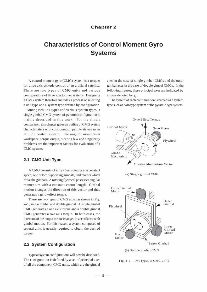
There are two types of CMG units, as shown in Fig.2–1, single gimbal and double gimbal. A single gimbal
CMG generates a one axis torque and a double gimbal
CMG generates a two axis torque. In both cases, thedirection of the output torque changes in accordance with
gimbal motion. For this reason, a system composed of
several units is usually required to obtain the desiredtorque.
2.2 System Configuration
Typical system configurations will now be discussed.
The configuration is defined by a set of principal axesof all the component CMG units, which are the gimbal
axes in the case of single gimbal CMGs and the outergimbal axes in the case of double gimbal CMGs. In the
following figures, these principal axes are indicated by
arrows denoted by gi .The system of each configuration is named as a system
type such as twin type system or the pyramid type system.
Chapter 2
Characteristics of Control Moment GyroSystems
Fig. 2–1 Two types of CMG units
Flywheel
Gyro Motor
(a) Single gimbal CMG
Gimbal Motor
Gimbal Mechanism
Gyro Effect Torque
Angular Momentum Vector
T
ω
AAAA
Gyro Motor
Inner Gimbal Motor
Outer Gimbal
Inner Gimbal
Outer Gimbal Motor
(b) Double gimbal CMG
AAAA
AFlywheel
AA
––– 6 –––
–– Technical Report of Mechanical Engineering Laboratory No.175 ––
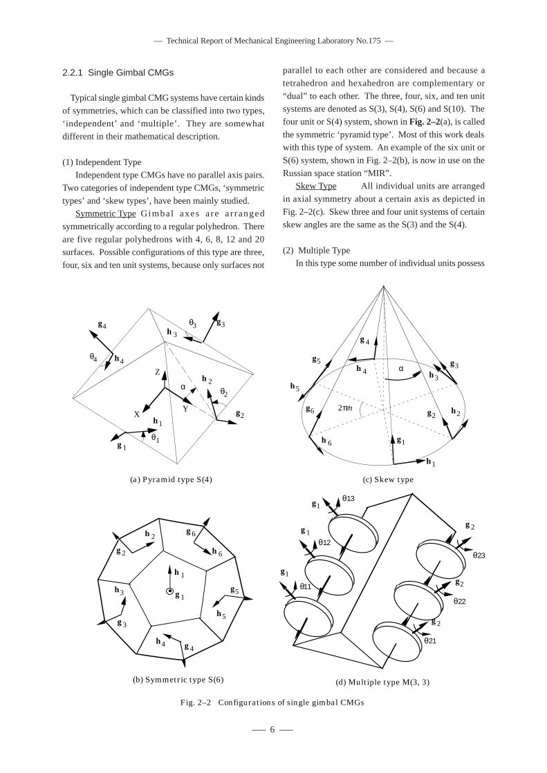
2.2.1 Single Gimbal CMGs
Typical single gimbal CMG systems have certain kinds
of symmetries, which can be classified into two types,
‘independent’ and ‘multiple’. They are somewhatdifferent in their mathematical description.
(1) Independent TypeIndependent type CMGs have no parallel axis pairs.
Two categories of independent type CMGs, ‘symmetric
types’ and ‘skew types’, have been mainly studied.Symmetric Type Gimbal axes are ar ranged
symmetrically according to a regular polyhedron. There
are five regular polyhedrons with 4, 6, 8, 12 and 20surfaces. Possible configurations of this type are three,
four, six and ten unit systems, because only surfaces not
parallel to each other are considered and because a
tetrahedron and hexahedron are complementary or
“dual” to each other. The three, four, six, and ten unitsystems are denoted as S(3), S(4), S(6) and S(10). The
four unit or S(4) system, shown in Fig. 2–2(a), is called
the symmetric ‘pyramid type’. Most of this work dealswith this type of system. An example of the six unit or
S(6) system, shown in Fig. 2–2(b), is now in use on the
Russian space station “MIR”.Skew Type All individual units are arranged
in axial symmetry about a certain axis as depicted in
Fig. 2–2(c). Skew three and four unit systems of certainskew angles are the same as the S(3) and the S(4).
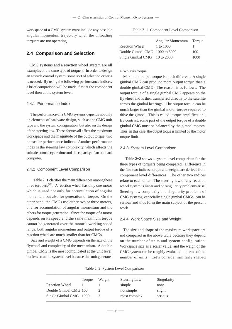
(2) Multiple TypeIn this type some number of individual units possess
XY
Z
g1
g2
g3g4
h4
θ1
θ4
h1
h2
h3
θ2
θ3
α
(a) Pyramid type S(4)
Fig. 2–2 Configurations of single gimbal CMGs
g2
g1
g3
g4
g5
g6
h1
h6
h5
h4
h3
h2
(b) Symmetric type S(6)
g1
g1
g1
g2
g2
g2
(d) Multiple type M(3, 3)
θ11
θ12
θ13
θ21
θ22
θ23
g1
h1
g2
g3
g4
g5
g6 h2
h3h4
h5
h6
α
2π⁄n
(c) Skew type
––– 7 –––
–– 2. Characteristics of Control Moment Gyro Systems ––
identical gimbal directions. These are denoted as M(m1,
m2, ...) hereafter, where mi is the number of the units
with the same gimbal direction. As an example, thesystem in Fig. 2–2(d) is denoted by M(3,3). A similar
system called ‘roof type’15, 16) would be denoted as
M(2,2) with this notation.
2.2.2 Two Dimensional System and Twin Type
System
A single gimbal CMG system of an arbitrary number
of units all having a common gimbal direction will be
called a two dimensional system in this work. In such asystem, the angular momentum vector and output torque
vector are always on a certain plane normal to the gimbal
direction. Though this type of system is not ordinarilyused by itself for attitude control, it can easily be
visualized and understood. It is, therefore, used for some
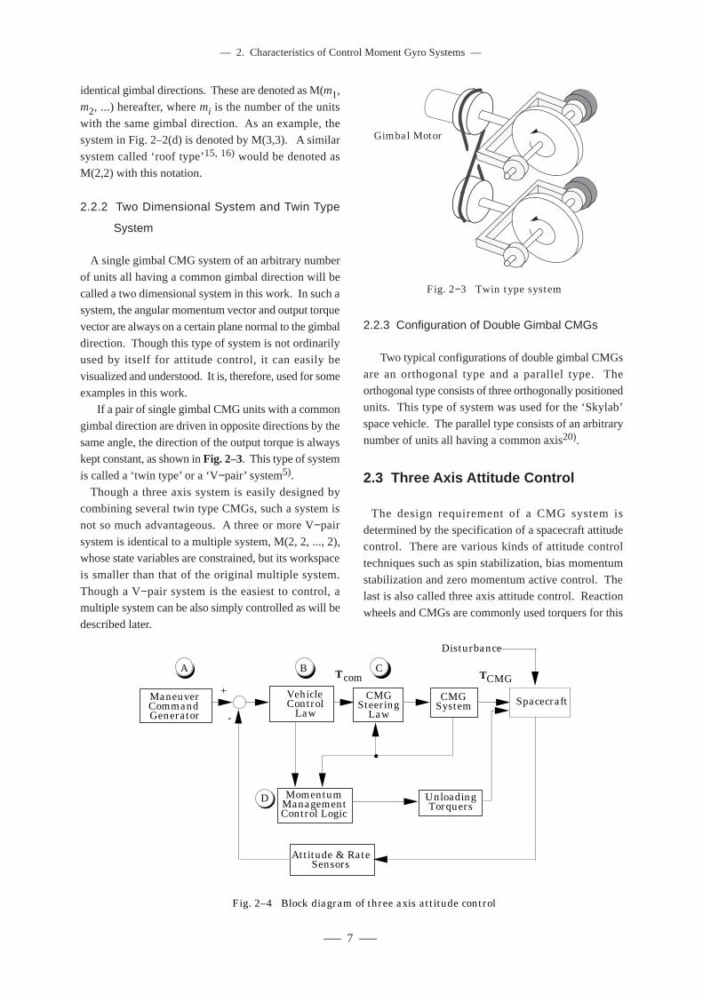
examples in this work.If a pair of single gimbal CMG units with a common
gimbal direction are driven in opposite directions by the
same angle, the direction of the output torque is alwayskept constant, as shown in Fig. 2–3. This type of system
is called a ‘twin type’ or a ‘V−pair’ system5).
Though a three axis system is easily designed bycombining several twin type CMGs, such a system is
not so much advantageous. A three or more V−pair
system is identical to a multiple system, M(2, 2, ..., 2),whose state variables are constrained, but its workspace
is smaller than that of the original multiple system.
Though a V−pair system is the easiest to control, amultiple system can be also simply controlled as will be
described later.
2.2.3 Configuration of Double Gimbal CMGs
Two typical configurations of double gimbal CMGs
are an orthogonal type and a parallel type. Theorthogonal type consists of three orthogonally positioned
units. This type of system was used for the ‘Skylab’
space vehicle. The parallel type consists of an arbitrarynumber of units all having a common axis20).
2.3 Three Axis Attitude Control
The design requirement of a CMG system is
determined by the specification of a spacecraft attitudecontrol. There are various kinds of attitude control
techniques such as spin stabilization, bias momentum
stabilization and zero momentum active control. Thelast is also called three axis attitude control. Reaction
wheels and CMGs are commonly used torquers for this
Fig. 2−3 Twin type system
Gimbal Motor
Attitude & RateSensors
MomentumManagementControl Logic
A B C
D
Tcom TCMG
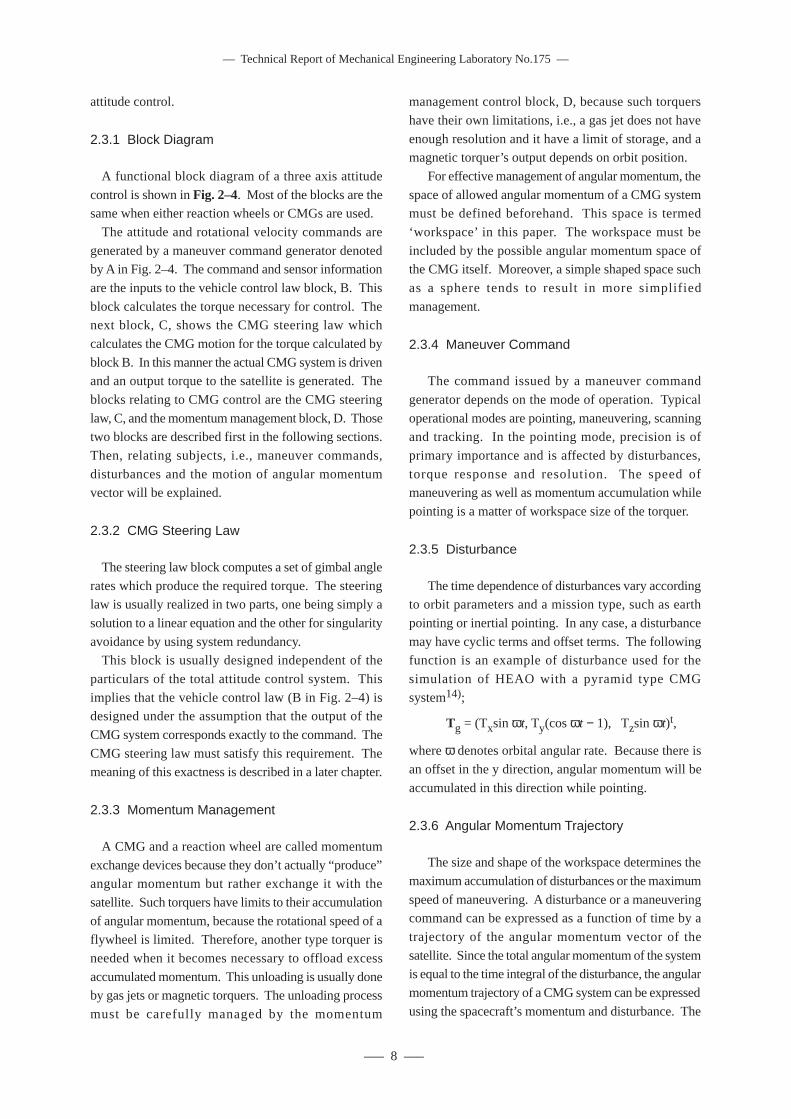
Fig. 2–4 Block diagram of three axis attitude control
ManeuverCommandGenerator
CMGSteering
Law
CMGSystem Spacecraft
+
-
VehicleControl
Law
Disturbance
UnloadingTorquers
––– 8 –––
–– Technical Report of Mechanical Engineering Laboratory No.175 ––
attitude control.
2.3.1 Block Diagram
A functional block diagram of a three axis attitude
control is shown in Fig. 2–4. Most of the blocks are thesame when either reaction wheels or CMGs are used.
The attitude and rotational velocity commands are
generated by a maneuver command generator denotedby A in Fig. 2–4. The command and sensor information
are the inputs to the vehicle control law block, B. This
block calculates the torque necessary for control. Thenext block, C, shows the CMG steering law which
calculates the CMG motion for the torque calculated by
block B. In this manner the actual CMG system is drivenand an output torque to the satellite is generated. The
blocks relating to CMG control are the CMG steering
law, C, and the momentum management block, D. Thosetwo blocks are described first in the following sections.
Then, relating subjects, i.e., maneuver commands,
disturbances and the motion of angular momentumvector will be explained.
2.3.2 CMG Steering Law
The steering law block computes a set of gimbal angle
rates which produce the required torque. The steeringlaw is usually realized in two parts, one being simply a
solution to a linear equation and the other for singularity
avoidance by using system redundancy.This block is usually designed independent of the
particulars of the total attitude control system. This
implies that the vehicle control law (B in Fig. 2–4) isdesigned under the assumption that the output of the
CMG system corresponds exactly to the command. The
CMG steering law must satisfy this requirement. Themeaning of this exactness is described in a later chapter.
2.3.3 Momentum Management
A CMG and a reaction wheel are called momentum
exchange devices because they don’t actually “produce”angular momentum but rather exchange it with the
satellite. Such torquers have limits to their accumulation
of angular momentum, because the rotational speed of aflywheel is limited. Therefore, another type torquer is
needed when it becomes necessary to offload excess
accumulated momentum. This unloading is usually doneby gas jets or magnetic torquers. The unloading process
must be carefully managed by the momentum
management control block, D, because such torquers
have their own limitations, i.e., a gas jet does not have
enough resolution and it have a limit of storage, and amagnetic torquer’s output depends on orbit position.
For effective management of angular momentum, the
space of allowed angular momentum of a CMG systemmust be defined beforehand. This space is termed
‘workspace’ in this paper. The workspace must be
included by the possible angular momentum space ofthe CMG itself. Moreover, a simple shaped space such
as a sphere tends to result in more simplified
management.
2.3.4 Maneuver Command
The command issued by a maneuver command
generator depends on the mode of operation. Typical
operational modes are pointing, maneuvering, scanningand tracking. In the pointing mode, precision is of
primary importance and is affected by disturbances,
torque response and resolution. The speed ofmaneuvering as well as momentum accumulation while
pointing is a matter of workspace size of the torquer.
2.3.5 Disturbance
The time dependence of disturbances vary accordingto orbit parameters and a mission type, such as earth
pointing or inertial pointing. In any case, a disturbance
may have cyclic terms and offset terms. The followingfunction is an example of disturbance used for the
simulation of HEAO with a pyramid type CMG
system14);
Tg = (Txsin ωt, Ty(cos ωt − 1), Tzsin ωt)t,
where ω denotes orbital angular rate. Because there is
an offset in the y direction, angular momentum will be
accumulated in this direction while pointing.
2.3.6 Angular Momentum Trajectory
The size and shape of the workspace determines the
maximum accumulation of disturbances or the maximum
speed of maneuvering. A disturbance or a maneuveringcommand can be expressed as a function of time by a
trajectory of the angular momentum vector of the
satellite. Since the total angular momentum of the systemis equal to the time integral of the disturbance, the angular
momentum trajectory of a CMG system can be expressed
using the spacecraft’s momentum and disturbance. The
––– 9 –––
–– 2. Characteristics of Control Moment Gyro Systems ––
Table 2–2 System Level Comparison
––––––––––––––––––––––––––––––––––––––––––––––––––––––––––––––––––––––––––
Torque Weight Steering Law SingularityReaction Wheel 1 1 simple none
Double Gimbal CMG 100 2 not simple slight
Single Gimbal CMG 1000 2 most complex serious––––––––––––––––––––––––––––––––––––––––––––––––––––––––––––––––––––––––––
Table 2–1 Component Level Comparison
––––––––––––––––––––––––––––––––––––––––––––
Angular Momentum TorqueReaction Wheel 1 to 1000 1
Double Gimbal CMG 1000 to 3000 100
Single Gimbal CMG 10 to 2000 1000––––––––––––––––––––––––––––––––––––––––––––
workspace of a CMG system must include any possible
angular momentum trajectory when the unloading
torquers are not operating.
2.4 Comparison and Selection
CMG systems and a reaction wheel system are all
examples of the same type of torquers. In order to design
an attitude control system, some sort of selection criteriais needed. By using the following performance indices,
a brief comparison will be made, first at the component
level then at the system level.
2.4.1 Performance Index
The performance of a CMG systems depends not only
on elements of hardware design, such as the CMG unit
type and the system configuration, but also on the designof the steering law. These factors all affect the maximum
workspace and the magnitude of the output torque, two
nonscalar performance indices. Another performanceindex is the steering law complexity, which affects the
attitude control cycle time and the capacity of an onboard
computer.
2.4.2 Component Level Comparison
Table 2−1 clarifies the main differences among these
three torquers64). A reaction wheel has only one motor
which is used not only for accumulation of angularmomentum but also for generation of torque. On the
other hand, the CMGs use either two or three motors,
one for accumulation of angular momentum and theothers for torque generation. Since the torque of a motor
depends on its speed and the same maximum torque
cannot be generated over the motor’s working speedrange, both angular momentum and output torque of a
reaction wheel are much smaller than for CMGs.
Size and weight of a CMG depends on the size of theflywheel and complexity of the mechanism. A double
gimbal CMG is the most complicated at the unit level,
but less so at the system level because this unit generates
a two axis torque.
Maximum output torque is much different. A singlegimbal CMG can produce more output torque than a
double gimbal CMG. The reason is as follows. The
output torque of a single gimbal CMG appears on theflywheel and is then transferred directly to the satellite
across the gimbal bearings. The output torque can be
much larger than the gimbal motor torque required todrive the gimbal. This is called ‘torque amplification’.
By contrast, some part of the output torque of a double
gimbal CMG must be balanced by the gimbal motors.Thus, in this case, the output toque is limited by the motor
torque limit.
2.4.3 System Level Comparison
Table 2−2 shows a system level comparison for thethree types of torquers being compared. Difference in
the first two indices, torque and weight, are derived from
component level differences. The other two indicesrelate to each other. The steering law of any reaction
wheel system is linear and no singularity problems arise.
Steering law complexity and singularity problems ofCMG systems, especially single gimbal CMGs, can be
serious and thus form the main subject of the present
work.
2.4.4 Work Space Size and Weight
The size and shape of the maximum workspace are
not compared in the above table because they depend
on the number of units and system configuration.Workspace size as a scalar value, and the weigh of the
CMG system can be roughly evaluated in terms of the
number of units. Let’s consider similarly shaped
––– 10 –––
–– Technical Report of Mechanical Engineering Laboratory No.175 ––
flywheels of diameter d and thickness t. Similarity
implies t ∝ d. Then, the weight and the size of maximum
workspace of an n unit system, denoted as W and H,follow the following relation if the rotational rate of the
gyro is the same:
W ∝ n d2 t ∝ n d3, (2–1)
H ∝ n ∫ (t d d2) dr ∝ n d5 . (2–2)
If H is set constant, W is given by;
W ∝ n d3 ∝ n 2/5 . (2–3)
This implies that the system with fewer units is lighter
but can still realize the same workspace size. Despite
the fact that other factors are ignored in estimating the
weight, it can generally be concluded that the systemsof less units have advantages in weight.
In this evaluation, it is assumed that the size of the
work space is proportional to the number of units by thesame multiplier for any system. From the comparison
in Chapter 9, this is almost true for systems of no less
than 6 units in the case of single gimbal CMGs. This,however, is not true in the case of less that 6 units.
Therefore it is better to evaluate some configuration
composed of 4 to 6 units.
––– 11 –––
–– 3. General Formulation ––
Chapter 3
General Formulation
This chapter first defines vectors, variables and
parameters of a single gimbal CMG system in an
arbitrary configuration, after which a basicmathematical descript ion of several system
characteristics are made. These characteristics are the
kinematic equation, the steering law, the torque outputperformance index, and singularity avoidance. The
shape of the maximum workspace and singularity
problem are described in the next chapter. Similardescriptions for double gimbal systems are given in
Appendix A.
3.1 Angular Momentum and Torque
A generalized system is considered consisting of n
identically sized single gimbal CMG units. The number
n is not less than 3 to enable three axis control. The
system configuration is defined by the relativearrangement of the gimbal directions. The system state
is defined by the set of all gimbal angles, each of which
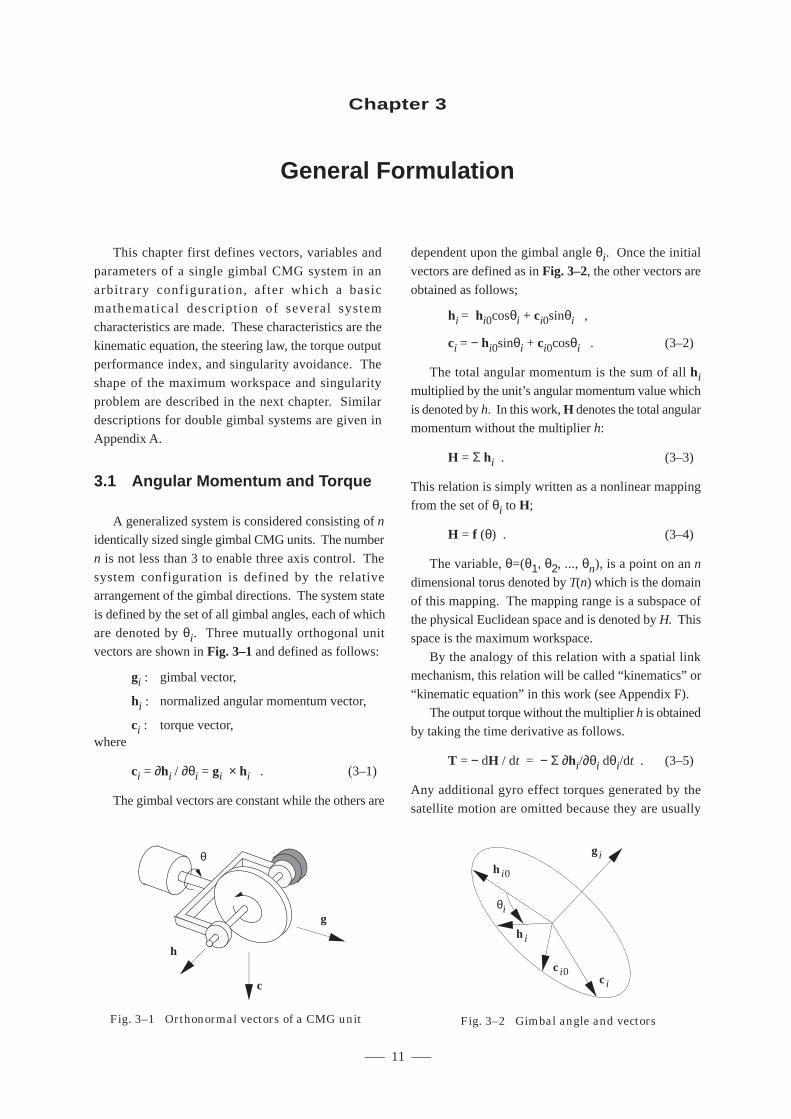
are denoted by θi. Three mutually orthogonal unitvectors are shown in Fig. 3–1 and defined as follows:
gi : gimbal vector,
hi : normalized angular momentum vector,
ci : torque vector,where
ci = ∂hi / ∂θi = gi × hi . (3–1)
The gimbal vectors are constant while the others are
dependent upon the gimbal angle θi. Once the initial
vectors are defined as in Fig. 3–2, the other vectors are
obtained as follows;
hi = hi0cosθi + ci0sinθi ,
ci = − hi0sinθi + ci0cosθi . (3–2)
The total angular momentum is the sum of all himultiplied by the unit’s angular momentum value which
is denoted by h. In this work, H denotes the total angularmomentum without the multiplier h:
H = Σ hi . (3–3)
This relation is simply written as a nonlinear mapping
from the set of θi to H;
H = f (θ) . (3–4)
The variable, θ=(θ1, θ2, ..., θn), is a point on an n
dimensional torus denoted by T(n) which is the domain
of this mapping. The mapping range is a subspace ofthe physical Euclidean space and is denoted by H. This
space is the maximum workspace.
By the analogy of this relation with a spatial linkmechanism, this relation will be called “kinematics” or
“kinematic equation” in this work (see Appendix F).
The output torque without the multiplier h is obtainedby taking the time derivative as follows.
T = − dH / dt = − Σ ∂hi/∂θi dθi/dt . (3–5)
Any additional gyro effect torques generated by the
satellite motion are omitted because they are usually
θ
h
c
g
Fig. 3–1 Orthonormal vectors of a CMG unit
ci
ci0
hi
hi0
gi
θi
Fig. 3–2 Gimbal angle and vectors
––– 12 –––
–– Technical Report of Mechanical Engineering Laboratory No.175 ––
treated in the overall satellite system dynamics, which
includes the CMG system (see Chapter 8).
Because the total output torque is a sum of output ofeach unit, it is also given as,
T = − Σ ci ωi
= − C ω , (3–6)
where
ωi = dθi/dt, and ω = (ω1, ω2, ..... , ωn)t .
(3–7)
The variable ωi is the rotational rate of each gimbal.The vector ω is a component vector of a tangent space
of T(n). The matrix C is a Jacobian of Eq. 3–4 and is
given by,
C = (c1 c2 .... cn) . (3–8)
As the unit’s angular momentum value is omitted in
Eqs. 3–5 and 3–6, the real output is obtained by
multiplying h.
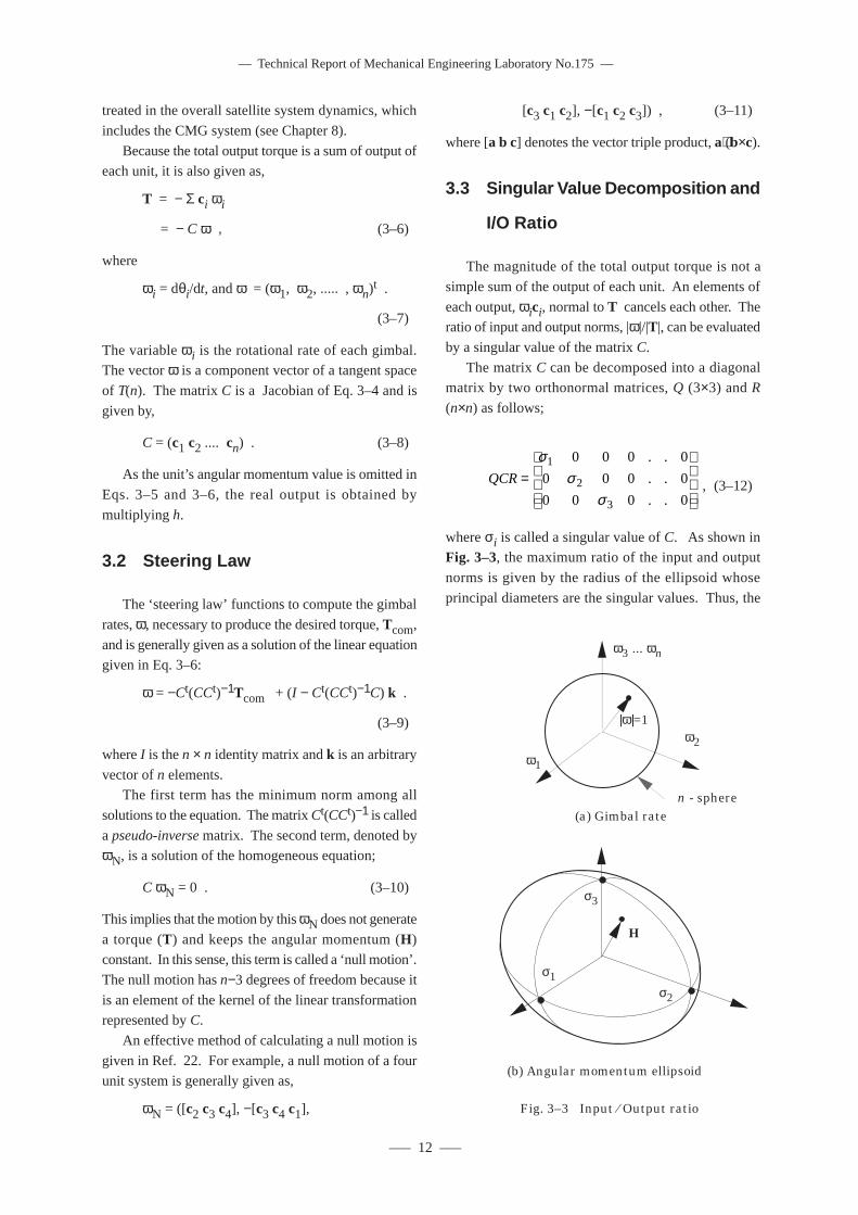
3.2 Steering Law
The ‘steering law’ functions to compute the gimbal
rates, ω, necessary to produce the desired torque, Tcom,
and is generally given as a solution of the linear equationgiven in Eq. 3–6:
ω = −Ct(CCt)−1Tcom + (I − Ct(CCt)−1C) k .
(3–9)
where I is the n × n identity matrix and k is an arbitrary
vector of n elements.The first term has the minimum norm among all
solutions to the equation. The matrix Ct(CCt)−1 is called
a pseudo-inverse matrix. The second term, denoted byωN, is a solution of the homogeneous equation;
C ωN = 0 . (3–10)
This implies that the motion by this ωN does not generate
a torque (T) and keeps the angular momentum (H)constant. In this sense, this term is called a ‘null motion’.
The null motion has n−3 degrees of freedom because it
is an element of the kernel of the linear transformationrepresented by C.
An effective method of calculating a null motion is
given in Ref. 22. For example, a null motion of a fourunit system is generally given as,
ωN = ([c2 c3 c4], −[c3 c4 c1],
[c3 c1 c2], −[c1 c2 c3]) , (3–11)
where [a b c] denotes the vector triple product, a⋅(b×c).
3.3 Singular Value Decomposition and
I/O Ratio
The magnitude of the total output torque is not a
simple sum of the output of each unit. An elements of
each output, ωici, normal to T cancels each other. Theratio of input and output norms, |ω|/|T|, can be evaluated
by a singular value of the matrix C.
The matrix C can be decomposed into a diagonalmatrix by two orthonormal matrices, Q (3×3) and R
(n×n) as follows;
QCR =
σσ
σ
1
2
3
0 0 0 0
0 0 0 0
0 0 0 0
. .
. .
. . , (3–12)
where σi is called a singular value of C. As shown inFig. 3–3, the maximum ratio of the input and output
norms is given by the radius of the ellipsoid whose
principal diameters are the singular values. Thus, the
Fig. 3–3 Input ⁄ Output ratio
(b) Angular momentum ellipsoid
(a) Gimbal rate
ω1
ω2
ω3 ... ωn
n - sphere
|ω|=1
σ1σ2
σ3
H
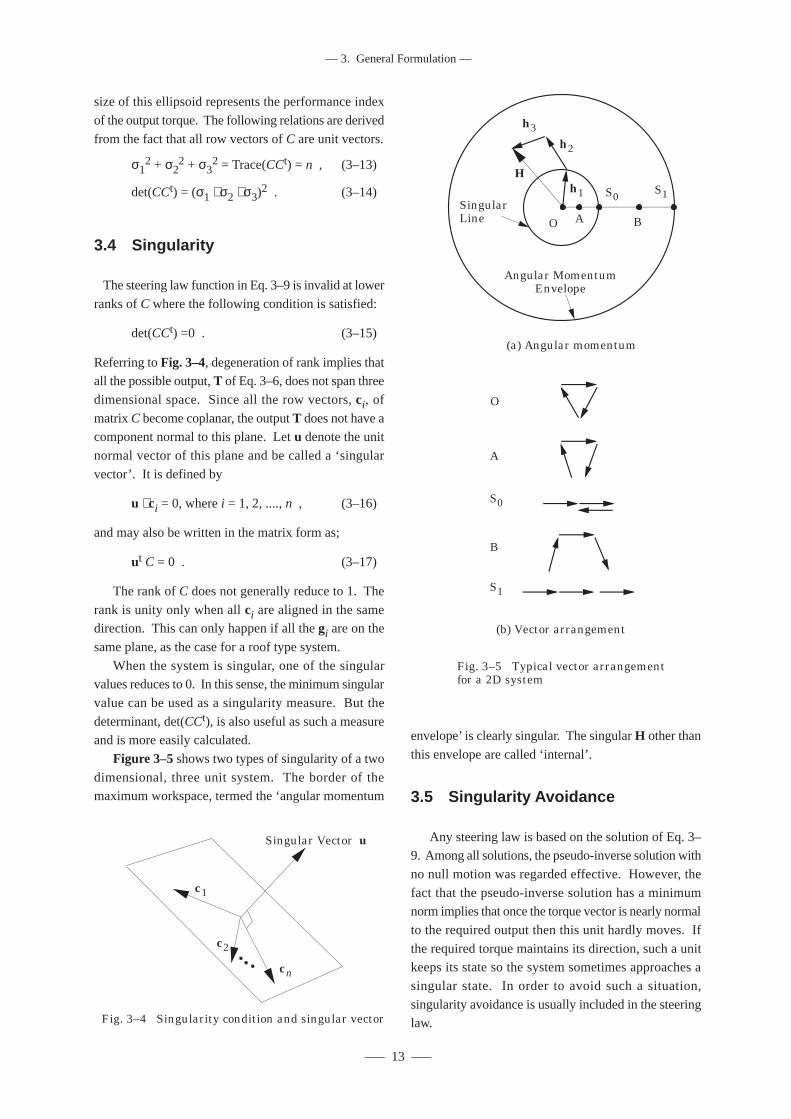
––– 13 –––
–– 3. General Formulation ––
size of this ellipsoid represents the performance index
of the output torque. The following relations are derived
from the fact that all row vectors of C are unit vectors.
σ12 + σ2
2 + σ32 = Trace(CCt) = n , (3–13)
det(CCt) = (σ1 ⋅ σ2 ⋅ σ3)2 . (3–14)
3.4 Singularity
The steering law function in Eq. 3–9 is invalid at lower
ranks of C where the following condition is satisfied:
det(CCt) =0 . (3–15)
Referring to Fig. 3–4, degeneration of rank implies thatall the possible output, T of Eq. 3–6, does not span three
dimensional space. Since all the row vectors, ci, of
matrix C become coplanar, the output T does not have acomponent normal to this plane. Let u denote the unit
normal vector of this plane and be called a ‘singular
vector’. It is defined by
u ⋅ ci = 0, where i = 1, 2, ...., n , (3–16)
and may also be written in the matrix form as;
ut C = 0 . (3–17)
The rank of C does not generally reduce to 1. The
rank is unity only when all ci are aligned in the samedirection. This can only happen if all the gi are on the
same plane, as the case for a roof type system.
When the system is singular, one of the singularvalues reduces to 0. In this sense, the minimum singular
value can be used as a singularity measure. But the
determinant, det(CCt), is also useful as such a measureand is more easily calculated.
Figure 3–5 shows two types of singularity of a two
dimensional, three unit system. The border of themaximum workspace, termed the ‘angular momentum
envelope’ is clearly singular. The singular H other than
this envelope are called ‘internal’.
3.5 Singularity Avoidance
Any steering law is based on the solution of Eq. 3–9. Among all solutions, the pseudo-inverse solution with
no null motion was regarded effective. However, the
fact that the pseudo-inverse solution has a minimumnorm implies that once the torque vector is nearly normal
to the required output then this unit hardly moves. If
the required torque maintains its direction, such a unitkeeps its state so the system sometimes approaches a
singular state. In order to avoid such a situation,
singularity avoidance is usually included in the steeringlaw.Fig. 3–4 Singularity condition and singular vector
c1
c2
cn
Singular Vector u
Fig. 3–5 Typical vector arrangement for a 2D system
(a) Angular momentum
O
B
A
S0
S1
(b) Vector arrangement
S1S0
O
h1
h2
h3
H
Angular Momentum Envelope
Singular Line A B
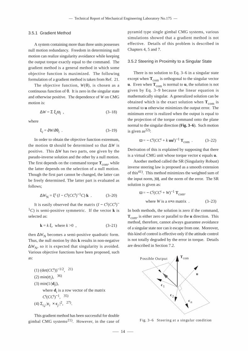
––– 14 –––
–– Technical Report of Mechanical Engineering Laboratory No.175 ––
3.5.1 Gradient Method
A system containing more than three units possesses
null motion redundancy. Freedom in determining null
motion can realize singularity avoidance while keepingthe output torque exactly equal to the command. The
gradient method is a general method in which some
objective function is maximized. The followingformulation of a gradient method is taken from Ref. 21.
The objective function, W(θ), is chosen as a
continuous function of θ. It is zero in the singular stateand otherwise positive. The dependence of W on CMG
motion is:
∆W = Σ ξiωi , (3–18)
where
ξi = ∂W/∂θi . (3–19)
In order to obtain the objective function extremum,
the motion ω should be determined so that ∆W is
positive. This ∆W has two parts, one given by thepseudo-inverse solution and the other by a null motion.
The first depends on the command torque Tcom, while
the latter depends on the selection of a null motion.Though the first part cannot be changed, the latter can
be freely determined. The latter part is evaluated as
follows;
∆WN = ξt (I − Ct(CCt)−1C) k . (3–20)
It is easily observed that the matrix (I − Ct(CCt)−
1C) is semi-positive symmetric. If the vector k is
selected as:
k = k ξ, where k >0 , (3–21)
then ∆WN becomes a semi-positive quadratic form.
Thus, the null motion by this k results in non-negative
∆WN, so it is expected that singularity is avoided.Various objective functions have been proposed, such
as:
(1) (det(CCt))−1/2, 21)
(2) min(σi), 36)
(3) min(1/|di|),
where di is a row vector of the matrix
Ct(CCt)−1, 35)
(4) Σi,j |ci × cj |2, 27).
This gradient method has been successful for double
gimbal CMG systems21). However, in the case of
c1
u
c2cn
TcomPossible Output
Fig. 3–6 Steering at a singular condition
pyramid type single gimbal CMG systems, various
simulations showed that a gradient method is not
effective. Details of this problem is described inChapters 4, 5 and 7.
3.5.2 Steering in Proximity to a Singular State
There is no solution to Eq. 3–6 in a singular state
except when Tcom is orthogonal to the singular vectoru. Even when Tcom is normal to u, the solution is not
given by Eq. 3–9 because the linear equation is
mathematically singular. A generalized solution can beobtained which is the exact solution when Tcom is
normal to u otherwise minimizes the output error. The
minimum error is realized when the output is equal tothe projection of the torque command onto the plane
normal to the singular direction (Fig. 3–6). Such motion
is given as22):
ω = − Ct(CCt + k uut)−1 Tcom . (3–22)
Derivation of this is explained by supposing that there
is a virtual CMG unit whose torque vector c equals u.
Another method called the SR (Singularity Robust)inverse steering law is proposed as a smooth extension
of this41). This method minimizes the weighted sum of
the input norm, |ω|, and the norm of the error. The SRsolution is given as:
ω = − Ct(CCt + W)−1 Tcom,
where W is a n×n matrix . (3–23)
In both methods, the solution is zero if the command,
Tcom, is either zero or parallel to the u direction. Thismethod, therefore, cannot always guarantee avoidance
of a singular state nor can it escape from one. Moreover,
this kind of control is effective only if the attitude controlis not totally degraded by the error in torque. Details
are described in Section 7.2.
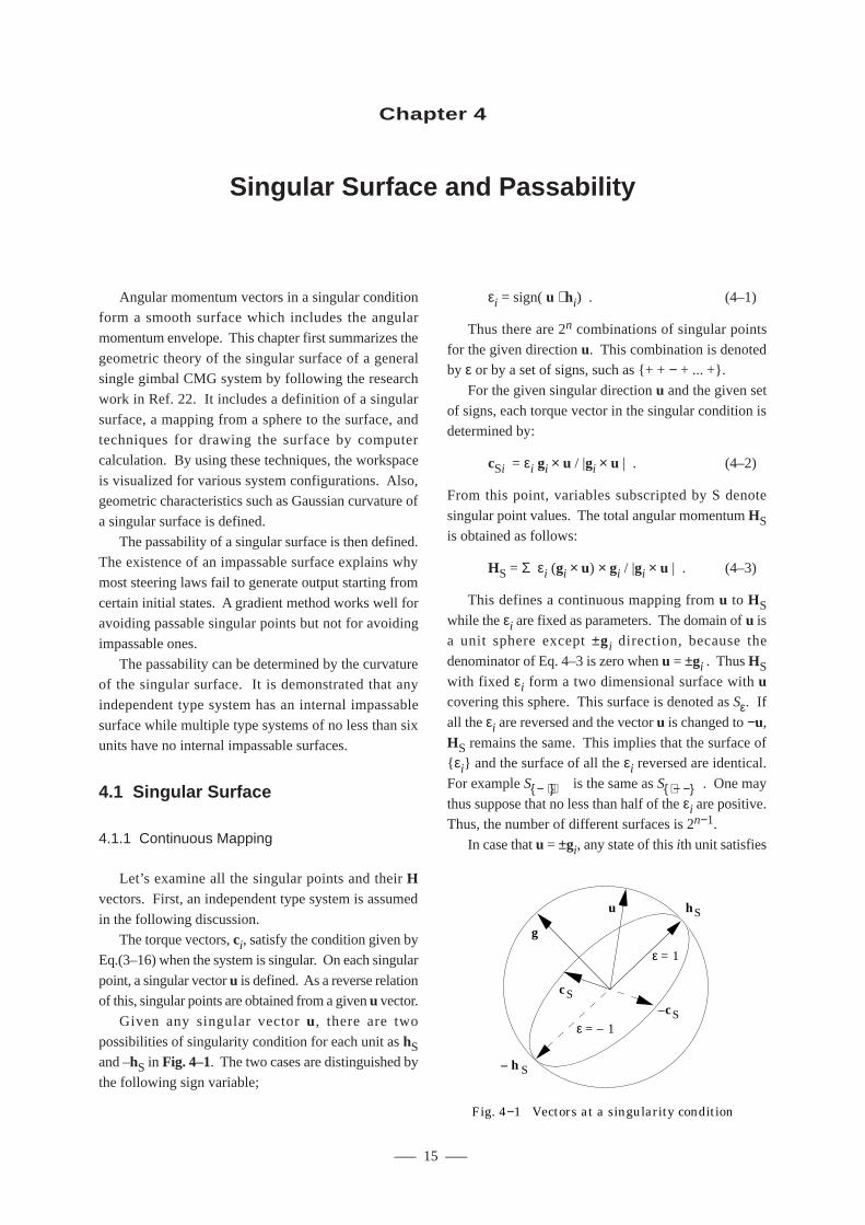
––– 15 –––
–– 4. Singular Surface and Passability ––
Angular momentum vectors in a singular conditionform a smooth surface which includes the angular
momentum envelope. This chapter first summarizes the
geometric theory of the singular surface of a generalsingle gimbal CMG system by following the research
work in Ref. 22. It includes a definition of a singular
surface, a mapping from a sphere to the surface, andtechniques for drawing the surface by computer
calculation. By using these techniques, the workspace
is visualized for various system configurations. Also,geometric characteristics such as Gaussian curvature of
a singular surface is defined.
The passability of a singular surface is then defined.The existence of an impassable surface explains why
most steering laws fail to generate output starting from
certain initial states. A gradient method works well foravoiding passable singular points but not for avoiding
impassable ones.
The passability can be determined by the curvatureof the singular surface. It is demonstrated that any
independent type system has an internal impassable
surface while multiple type systems of no less than sixunits have no internal impassable surfaces.
4.1 Singular Surface
4.1.1 Continuous Mapping
Let’s examine all the singular points and their Hvectors. First, an independent type system is assumed
in the following discussion.The torque vectors, ci, satisfy the condition given by
Eq.(3–16) when the system is singular. On each singular
point, a singular vector u is defined. As a reverse relationof this, singular points are obtained from a given u vector.
Given any singular vector u, there are two
possibilities of singularity condition for each unit as hSand –hS in Fig. 4–1. The two cases are distinguished by
the following sign variable;
εi = sign( u ⋅ hi) . (4–1)
Thus there are 2n combinations of singular points
for the given direction u. This combination is denotedby ε or by a set of signs, such as {+ + − + ... +}.
For the given singular direction u and the given set
of signs, each torque vector in the singular condition isdetermined by:
cSi = εi gi × u / |gi × u | . (4–2)
From this point, variables subscripted by S denote
singular point values. The total angular momentum HSis obtained as follows:
HS = Σ εi (gi × u) × gi / |gi × u | . (4–3)
This defines a continuous mapping from u to HSwhile the εi are fixed as parameters. The domain of u isa unit sphere except ±gi direction, because the
denominator of Eq. 4–3 is zero when u = ±gi . Thus HSwith fixed εi form a two dimensional surface with ucovering this sphere. This surface is denoted as Sε. If
all the εi are reversed and the vector u is changed to −u,
HS remains the same. This implies that the surface of{ εi} and the surface of all the εi reversed are identical.
For example S{− + +} is the same as S{+ − −}. One may
thus suppose that no less than half of the εi are positive.Thus, the number of different surfaces is 2n−1.
In case that u = ±gi, any state of this ith unit satisfies
Chapter 4
Singular Surface and Passability
Fig. 4−1 Vectors at a singularity condition
g
u hS
– hS
cS
ε = 1
ε = – 1–cS
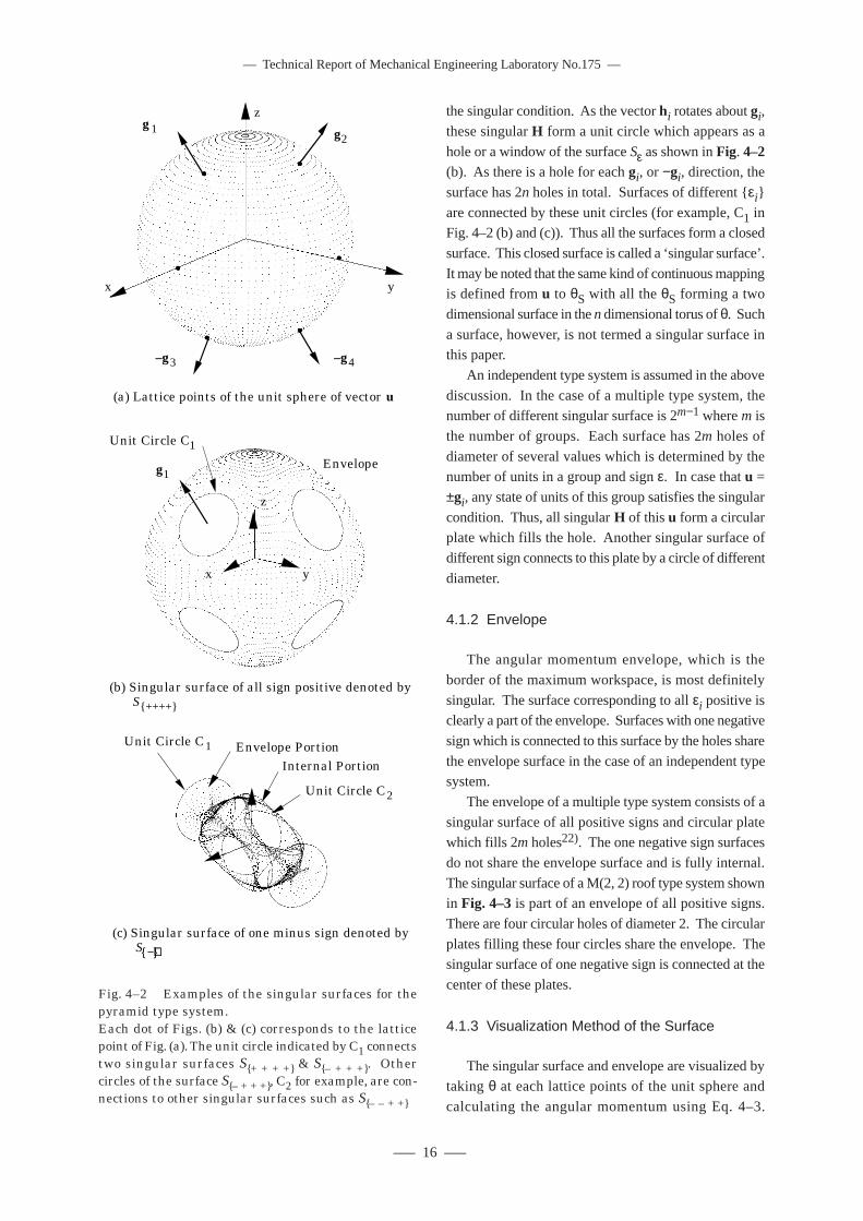
–– Technical Report of Mechanical Engineering Laboratory No.175 ––
––– 16 –––
the singular condition. As the vector hi rotates about gi,
these singular H form a unit circle which appears as a
hole or a window of the surface Sε as shown in Fig. 4–2(b). As there is a hole for each gi, or −gi, direction, the
surface has 2n holes in total. Surfaces of different {εi}
are connected by these unit circles (for example, C1 inFig. 4–2 (b) and (c)). Thus all the surfaces form a closed
surface. This closed surface is called a ‘singular surface’.
It may be noted that the same kind of continuous mappingis defined from u to θS with all the θS forming a two
dimensional surface in the n dimensional torus of θ. Such
a surface, however, is not termed a singular surface inthis paper.
An independent type system is assumed in the above
discussion. In the case of a multiple type system, thenumber of different singular surface is 2m−1 where m is
the number of groups. Each surface has 2m holes of
diameter of several values which is determined by thenumber of units in a group and sign ε. In case that u =
±gi, any state of units of this group satisfies the singular
condition. Thus, all singular H of this u form a circularplate which fills the hole. Another singular surface of
different sign connects to this plate by a circle of different
diameter.
4.1.2 Envelope
The angular momentum envelope, which is the
border of the maximum workspace, is most definitely
singular. The surface corresponding to all εi positive isclearly a part of the envelope. Surfaces with one negative
sign which is connected to this surface by the holes share
the envelope surface in the case of an independent typesystem.
The envelope of a multiple type system consists of a
singular surface of all positive signs and circular platewhich fills 2m holes22). The one negative sign surfaces
do not share the envelope surface and is fully internal.
The singular surface of a M(2, 2) roof type system shownin Fig. 4–3 is part of an envelope of all positive signs.
There are four circular holes of diameter 2. The circular
plates filling these four circles share the envelope. Thesingular surface of one negative sign is connected at the
center of these plates.
4.1.3 Visualization Method of the Surface
The singular surface and envelope are visualized bytaking θ at each lattice points of the unit sphere and
calculating the angular momentum using Eq. 4–3.
g1
Unit Circle C1
Envelope
x y
z
(b) Singular surface of all sign positive denoted by S{++++}
Unit Circle C1 Envelope PortionInternal Portion
Unit Circle C2
(c) Singular surface of one minus sign denoted by S{−+++}
(a) Lattice points of the unit sphere of vector u
g1 g2
–g3 –g4
x y
z
Fig. 4–2 Examples of the singular surfaces for thepyramid type system.Each dot of Figs. (b) & (c) corresponds to the latticepoint of Fig. (a). The unit circle indicated by C1 connectstwo singular surfaces S{+ + + +} & S{– + + +}. Othercircles of the surface S{– + + +}, C2 for example, are con-nections to other singular surfaces such as S{– – + +}
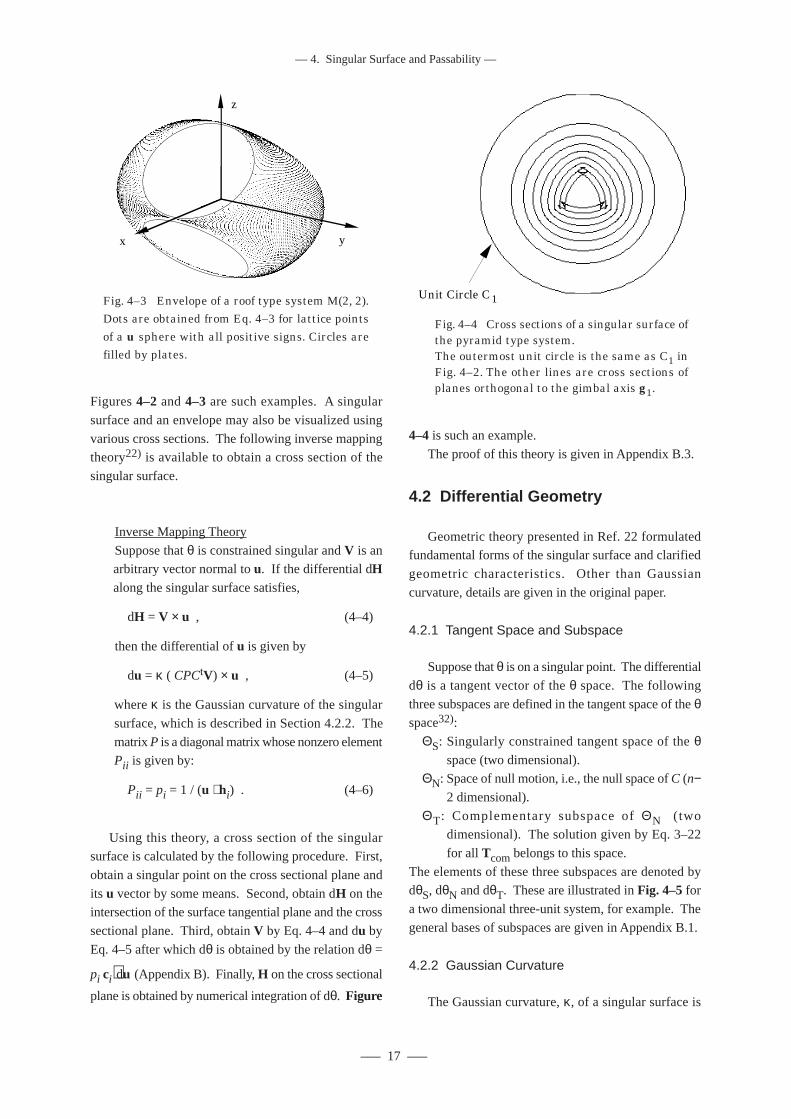
––– 17 –––
–– 4. Singular Surface and Passability ––
Figures 4–2 and 4–3 are such examples. A singular
surface and an envelope may also be visualized using
various cross sections. The following inverse mappingtheory22) is available to obtain a cross section of the
singular surface.
Inverse Mapping Theory
Suppose that θ is constrained singular and V is anarbitrary vector normal to u. If the differential dHalong the singular surface satisfies,
dH = V × u , (4–4)
then the differential of u is given by
du = κ ( CPCtV) × u , (4–5)
where κ is the Gaussian curvature of the singular
surface, which is described in Section 4.2.2. The
matrix P is a diagonal matrix whose nonzero elementPii is given by:
Pii = pi = 1 / (u ⋅ hi) . (4–6)
Using this theory, a cross section of the singularsurface is calculated by the following procedure. First,
obtain a singular point on the cross sectional plane and
its u vector by some means. Second, obtain dH on theintersection of the surface tangential plane and the cross
sectional plane. Third, obtain V by Eq. 4–4 and du by
Eq. 4–5 after which dθ is obtained by the relation dθ =
pi ci⋅du (Appendix B). Finally, H on the cross sectional
plane is obtained by numerical integration of dθ. Figure
4–4 is such an example.
The proof of this theory is given in Appendix B.3.
4.2 Differential Geometry
Geometric theory presented in Ref. 22 formulatedfundamental forms of the singular surface and clarified
geometric characteristics. Other than Gaussian
curvature, details are given in the original paper.
4.2.1 Tangent Space and Subspace
Suppose that θ is on a singular point. The differential
dθ is a tangent vector of the θ space. The following
three subspaces are defined in the tangent space of the θspace32):
ΘS: Singularly constrained tangent space of the θspace (two dimensional).
ΘN: Space of null motion, i.e., the null space of C (n−2 dimensional).
ΘT: Complementary subspace of ΘN (twodimensional). The solution given by Eq. 3–22
for all Tcom belongs to this space.
The elements of these three subspaces are denoted bydθS, dθN and dθT. These are illustrated in Fig. 4–5 for
a two dimensional three-unit system, for example. The
general bases of subspaces are given in Appendix B.1.
4.2.2 Gaussian Curvature
The Gaussian curvature, κ, of a singular surface is
x y
z
Fig. 4–3 Envelope of a roof type system M(2, 2).Dots are obtained from Eq. 4–3 for lattice pointsof a u sphere with all positive signs. Circles arefilled by plates.
Unit Circle C1
Fig. 4–4 Cross sections of a singular surface ofthe pyramid type system.The outermost unit circle is the same as C1 inFig. 4–2. The other lines are cross sections ofplanes orthogonal to the gimbal axis g1.
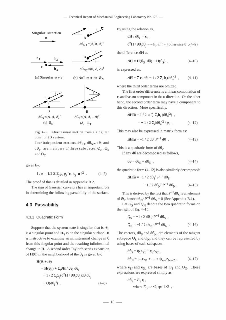
–– Technical Report of Mechanical Engineering Laboratory No.175 ––
––– 18 –––
given by:
1 / κ = 1/2 ΣiΣj pi pj [ci cj u ]2 . (4–7)
The proof of this is detailed in Appendix B.2.The sign of Gaussian curvature has an important role
in determining the following passability of the surface.
4.3 Passability
4.3.1 Quadratic Form
Suppose that the system state is singular, that is, θSis a singular point and HS is on the singular surface. It
is instructive to examine an infinitesimal change in θfrom this singular point and the resulting infinitesimalchange in H. A second order Taylor’s series expansion
of H(θ) in the neighborhood of the θS is given by:
H(θS+dθ)
= H(θS) + Σi∂H / ∂θi dθi
+ 1 / 2 ΣiΣj(∂2H / ∂θi∂θj)dθidθj
+ O(dθi3) . (4–8)
By using the relation as,
∂H / ∂θi = ci ,
∂2H / ∂θi∂θj = – hi, if i = j otherwise 0 ,(4–9)
the difference ∆H as
∆H = H(θS+dθ) − H(θS) , (4–10)
is expressed as,
∆H = Σ ci dθi − 1 / 2 Σi hi(dθi)2 , (4–11)
where the third order terms are omitted.
The first order difference is a linear combination of
ci and has no component in the u direction. On the otherhand, the second order term may have a component to
this direction. More specifically,
∆H⋅u = 1 / 2 u ⋅(–Σihi (dθi)2) ,
= − 1 / 2 Σi(dθi)2 / pi . (4–12)
This may also be expressed in matrix form as:
∆H⋅u = −1 / 2 dθt P−1 dθ . (4–13)
This is a quadratic form of dθi.
If any dθ are decomposed as follows,
dθ = dθS + dθN , (4–14)
the quadratic form (4–12) is also similarly decomposed:
∆H⋅u = −1 / 2 dθSt P−1 dθS
− 1 / 2 dθNt P−1 dθN . (4–15)
This is derived by the fact that P−1dθS is an element
of ΘT hence dθNt P−1 dθS = 0 (See Appendix B.1).
Let QS and QN denote the two quadratic forms onthe right of Eq. 4–15:
QS = −1 / 2 dθSt P−1 dθS ,
QN = −1 / 2 dθNt P−1 dθN . (4–16)
The vectors, dθS and dθN, are elements of the tangent
subspace ΘS and ΘN, and they can be represented byusing bases of each subspaces:
dθS = φ1eS1 + φ2eS2 ,
dθN = ψ1eN1 + ... + ψn-2eNn-2 , (4–17)
where eSi and eNi are bases of ΘS and ΘN. These
expressions are expressed simply as,
dθS = ES φ ,
where ES : n×2, φ : 1×2 ,
(a) Singular state
B
h1 h2
h3
uSingular Direction
dθN1=(∆, 0, ∆) t
dθN2=(0, ∆, ∆) t
(b) Null motion ΘN
B
B
dθS=(∆, ∆, ∆) t
(c) ΘS
B
dθT=(∆, ∆, – ∆) t
(d) ΘT
B
Fig. 4–5 Infinitesimal motion from a singularpoint of 2D system.
Four independent motions, dθN1, dθN2, dθS and
dθT, are members of three subspaces, ΘN, ΘS
and ΘT.
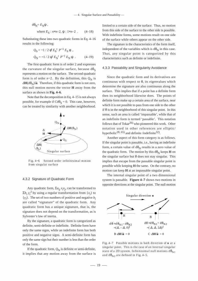
––– 19 –––
–– 4. Singular Surface and Passability ––
limited to a certain side of the surface. Thus, no motion
from this side of the surface to the other side is possible.
With indefinite forms, some motions result on one sideof the surface while others appear on the other side.
The signature is the characteristics of the form itself,
independent of the variables which is dθN in this case.Thus, any singular point is categorized by this
characteristics such as definite or indefinite.
4.3.3 Passability and Singularity Avoidance
Since the quadratic form and its derivatives arecontinuous with respect to θ, its eigenvalues which
determine the signature are also continuous along the
surface. This implies that if a point has a definite formthen its neighborhood likewise does. The points of
definite form make up a certain area of the surface, near
which it is not possible to pass from one side to the otherif θ is in the neighborhood of this singular point. In this
sense, such an area is called ‘impassable’, while that of
an indefinite form is termed ‘passable’. This notationfollows that of Tokar26) who pioneered this work. Other
notation used in other references are elliptic/
hyperbolic28, 65) and definite /indefinite32).Another aspect of this form category is as follows.
If the singular point is passable, i.e., having an indefinite
form, a certain value of dθN results in a zero value ofthe quadratic form. The motion by this dθN keeps H on
the singular surface but θ does not stay singular. This
implies that escape from the passable singular point ispossible while keeping H the same. On the contrary, no
motion can keep H at an impassable singular point.
The internal singular point of a two dimensionalsystem is passable. Figure 4–7 shows two motions in
opposite directions at the singular point. The null motion
dθN= ENψ ,
where ES : n×n–2, ψ : 1×n–2 . (4–18)
Substituting these into two quadratic forms in Eq. 4–16results in the following:
QS = −1 / 2 φt ESt P−1 ES φ ,
QN = −1 / 2 ψt ENt P−1 EN ψ . (4–19)
The first quadratic form is of order 2 and expresses
the curvature of the singular surface, because dθSrepresents a motion on the surface. The second quadratic
form is of order n−2. By the definition, this QN is
∆H(dθN)⋅u. Therefore, if this quadratic form is not zero,this null motion moves the vector H away from the
surface as shown in Fig. 4–6.Note that the decomposition in Eq. 4–15 is not always
possible, for example if CdθS = 0. This case, however,
can be treated by similarity with another neighborhood.
4.3.2 Signature of Quadratic Form
Any quadratic form, Σaij xixj, can be transformed to
Σbi yi2 by using a regular transformation from {xi} to
{yi}. The set of two numbers of positive and negative biare called “signature” of the quadratic form. Any
quadratic form has a unique signature, that is, the
signature does not depend on the transformation, as isSylvester’s law of inertia.
By the signature, a quadratic form is categorized as
definite, semi-definite or indefinite. Definite form haveonly the same signs, while an indefinite form has both
positive and negative signs. A semi-definite form has
only the same sign but their number is less than the orderof the form.
If the quadratic form, QN is definite or semi-definite,
it implies that any motion away from the surface is
B
dθ =dθN1– dθN2 =(∆, – ∆, 0)t
(a) ∆H⋅u < 0
Singular direction u
B
(b) ∆H⋅u > 0
dθ =dθN1+ dθN2 =( ∆, ∆, 2∆) t
Fig. 4–7 Possible motions in both direction of u at asingular point. This is the case of an internal singularstate of a 2D system. Infinitesimal null motions dθN1and dθN2 are defined in Fig. 4–5.
Fig. 4−6 Second order infinitesimal motionfrom singular surface
∆H
u
Singular surface
∆H(θN)
QN
∆H(θS)
QS
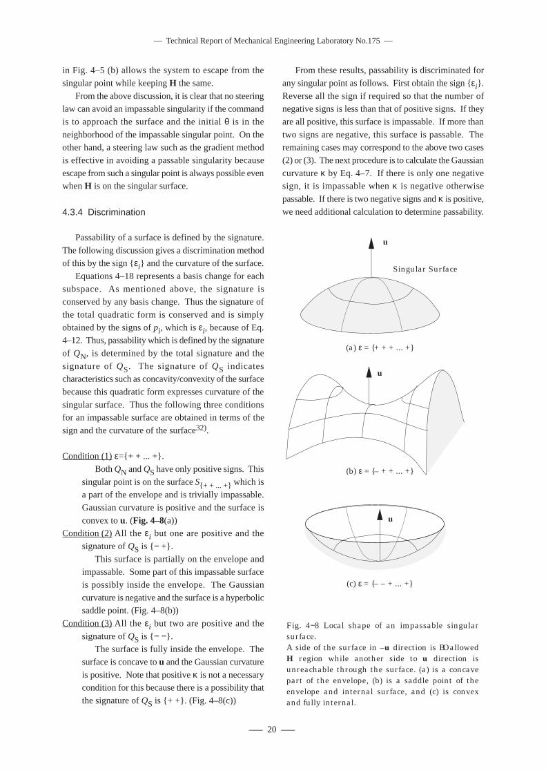
–– Technical Report of Mechanical Engineering Laboratory No.175 ––
––– 20 –––
in Fig. 4–5 (b) allows the system to escape from the
singular point while keeping H the same.
From the above discussion, it is clear that no steeringlaw can avoid an impassable singularity if the command
is to approach the surface and the initial θ is in the
neighborhood of the impassable singular point. On theother hand, a steering law such as the gradient method
is effective in avoiding a passable singularity because
escape from such a singular point is always possible evenwhen H is on the singular surface.
4.3.4 Discrimination
Passability of a surface is defined by the signature.
The following discussion gives a discrimination methodof this by the sign {εi} and the curvature of the surface.
Equations 4–18 represents a basis change for each
subspace. As mentioned above, the signature isconserved by any basis change. Thus the signature of
the total quadratic form is conserved and is simply
obtained by the signs of pi, which is εi, because of Eq.4–12. Thus, passability which is defined by the signature
of QN, is determined by the total signature and the
signature of QS. The signature of QS indicatescharacteristics such as concavity/convexity of the surface
because this quadratic form expresses curvature of the
singular surface. Thus the following three conditionsfor an impassable surface are obtained in terms of the
sign and the curvature of the surface32).
Condition (1)ε={+ + ... +}.
Both QN and QS have only positive signs. This
singular point is on the surface S{+ + ... +} which isa part of the envelope and is trivially impassable.
Gaussian curvature is positive and the surface is
convex to u. (Fig. 4–8(a))Condition (2)All the εi but one are positive and the
signature of QS is {− +}.
This surface is partially on the envelope andimpassable. Some part of this impassable surface
is possibly inside the envelope. The Gaussian
curvature is negative and the surface is a hyperbolicsaddle point. (Fig. 4–8(b))
Condition (3)All the εi but two are positive and the
signature of QS is {− −}.The surface is fully inside the envelope. The
surface is concave to u and the Gaussian curvature
is positive. Note that positive κ is not a necessarycondition for this because there is a possibility that
the signature of QS is {+ +}. (Fig. 4–8(c))
From these results, passability is discriminated for
any singular point as follows. First obtain the sign {εi}.
Reverse all the sign if required so that the number ofnegative signs is less than that of positive signs. If they
are all positive, this surface is impassable. If more than
two signs are negative, this surface is passable. Theremaining cases may correspond to the above two cases
(2) or (3). The next procedure is to calculate the Gaussian
curvature κ by Eq. 4–7. If there is only one negativesign, it is impassable when κ is negative otherwise
passable. If there is two negative signs and κ is positive,
we need additional calculation to determine passability.
Fig. 4−8 Local shape of an impassable singular surface. A side of the surface in –u direction is an allowed H region while another side to u direction is unreachable through the surface. (a) is a concave part of the envelope, (b) is a saddle point of the envelope and internal surface, and (c) is convex and fully internal.
(a) ε = {+ + + ... +}
u
Singular Surface
u
(b) ε = {– + + ... +}
(c) ε = {– – + ... +}
u
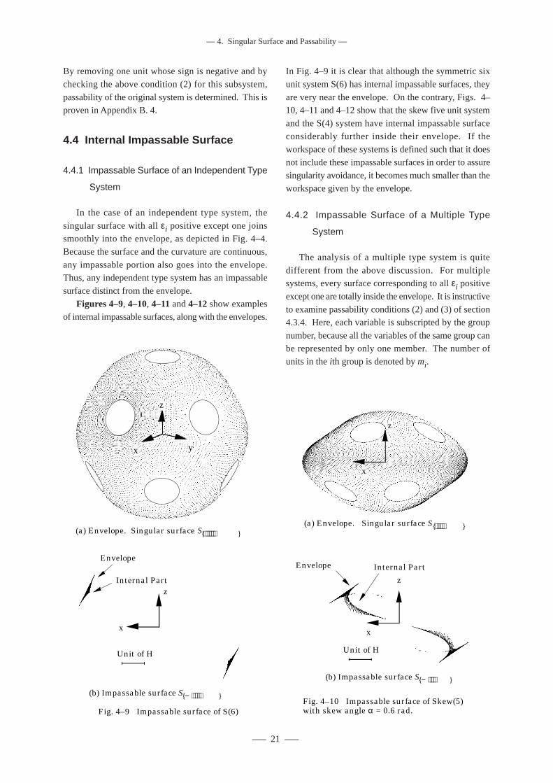
––– 21 –––
–– 4. Singular Surface and Passability ––
In Fig. 4–9 it is clear that although the symmetric six
unit system S(6) has internal impassable surfaces, they
are very near the envelope. On the contrary, Figs. 4–10, 4–11 and 4–12 show that the skew five unit system
and the S(4) system have internal impassable surface
considerably further inside their envelope. If theworkspace of these systems is defined such that it does
not include these impassable surfaces in order to assure
singularity avoidance, it becomes much smaller than theworkspace given by the envelope.
4.4.2 Impassable Surface of a Multiple Type
System
The analysis of a multiple type system is quite
different from the above discussion. For multiplesystems, every surface corresponding to all εi positive
except one are totally inside the envelope. It is instructive
to examine passability conditions (2) and (3) of section4.3.4. Here, each variable is subscripted by the group
number, because all the variables of the same group can
be represented by only one member. The number ofunits in the ith group is denoted by mi.
By removing one unit whose sign is negative and by
checking the above condition (2) for this subsystem,
passability of the original system is determined. This isproven in Appendix B. 4.
4.4 Internal Impassable Surface
4.4.1 Impassable Surface of an Independent Type
System
In the case of an independent type system, the
singular surface with all εi positive except one joinssmoothly into the envelope, as depicted in Fig. 4–4.
Because the surface and the curvature are continuous,
any impassable portion also goes into the envelope.Thus, any independent type system has an impassable
surface distinct from the envelope.
Figures 4–9, 4–10, 4–11 and 4–12 show examplesof internal impassable surfaces, along with the envelopes.
(a) Envelope. Singular surface S{+ + + + + +}
x y
z
Fig. 4–9 Impassable surface of S(6)
Unit of H
(b) Impassable surface S{− + + + + +}
x
z
Envelope
Internal Part
(a) Envelope. Singular surface S {+ + + + +}
x
z
Fig. 4–10 Impassable surface of Skew(5) with skew angle α = 0.6 rad.
Unit of H
(b) Impassable surface S{− + + + +}
x
z
Envelope Internal Part
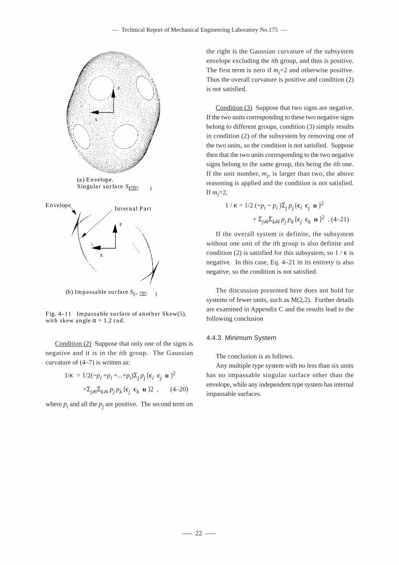
–– Technical Report of Mechanical Engineering Laboratory No.175 ––
––– 22 –––
the right is the Gaussian curvature of the subsystem
envelope excluding the ith group, and thus is positive.
The first term is zero if mi=2 and otherwise positive.Thus the overall curvature is positive and condition (2)
is not satisfied.
Condition (3) Suppose that two signs are negative.
If the two units corresponding to these two negative signs
belong to different groups, condition (3) simply resultsin condition (2) of the subsystem by removing one of
the two units, so the condition is not satisfied. Suppose
then that the two units corresponding to the two negativesigns belong to the same group, this being the ith one.
If the unit number, mi, is larger than two, the above
reasoning is applied and the condition is not satisfied.If mi=2,
1 / κ = 1/2 (−pi − pi )Σj pj [ci cj u ]2
+ Σj≠iΣk≠i pj pk [cj ck u ]2 . (4–21)
If the overall system is definite, the subsystem
without one unit of the ith group is also definite andcondition (2) is satisfied for this subsystem, so 1 / κ is
negative. In this case, Eq. 4–21 in its entirety is also
negative, so the condition is not satisfied.
The discussion presented here does not hold for
systems of fewer units, such as M(2,2). Further detailsare examined in Appendix C and the results lead to the
following conclusion
4.4.3 Minimum System
The conclusion is as follows.Any multiple type system with no less than six units
has no impassable singular surface other than the
envelope, while any independent type system has internalimpassable surfaces.
Fig. 4–11 Impassable surface of another Skew(5), with skew angle α = 1.2 rad.
(a) Envelope.Singular surface S{+ + + + +}
x
z
(b) Impassable surface S{− + + + +}
x
z
Envelope Internal Part
Condition (2) Suppose that only one of the signs isnegative and it is in the i th group. The Gaussian
curvature of (4–7) is written as:
1/κ = 1/2(−pi +pi +...+pi)Σj pj [ci cj u ]2
+Σj≠iΣk≠i pj pk [cj ck u ]2 , (4–20)
where pi and all the pj are positive. The second term on
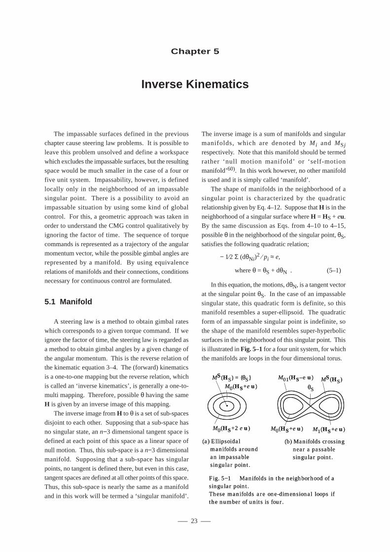
––– 23 –––
–– 5. Inverse Kinematics ––
The impassable surfaces defined in the previouschapter cause steering law problems. It is possible to
leave this problem unsolved and define a workspace
which excludes the impassable surfaces, but the resultingspace would be much smaller in the case of a four or
five unit system. Impassability, however, is defined
locally only in the neighborhood of an impassablesingular point. There is a possibility to avoid an
impassable situation by using some kind of global
control. For this, a geometric approach was taken inorder to understand the CMG control qualitatively by
ignoring the factor of time. The sequence of torque
commands is represented as a trajectory of the angularmomentum vector, while the possible gimbal angles are
represented by a manifold. By using equivalence
relations of manifolds and their connections, conditionsnecessary for continuous control are formulated.
5.1 Manifold
A steering law is a method to obtain gimbal rates
which corresponds to a given torque command. If weignore the factor of time, the steering law is regarded as
a method to obtain gimbal angles by a given change of
the angular momentum. This is the reverse relation ofthe kinematic equation 3–4. The (forward) kinematics
is a one-to-one mapping but the reverse relation, which
is called an ‘inverse kinematics’, is generally a one-to-multi mapping. Therefore, possible θ having the same
H is given by an inverse image of this mapping.
The inverse image from H to θ is a set of sub-spacesdisjoint to each other. Supposing that a sub-space has
no singular state, an n−3 dimensional tangent space is
defined at each point of this space as a linear space ofnull motion. Thus, this sub-space is a n−3 dimensional
manifold. Supposing that a sub-space has singular
points, no tangent is defined there, but even in this case,tangent spaces are defined at all other points of this space.
Thus, this sub-space is nearly the same as a manifold
and in this work will be termed a ‘singular manifold’.
Chapter 5
Inverse Kinematics
The inverse image is a sum of manifolds and singularmanifolds, which are denoted by M i and MSjrespectively. Note that this manifold should be termed
rather ‘null motion manifold’ or ‘self-motionmanifold’60). In this work however, no other manifold
is used and it is simply called ‘manifold’.
The shape of manifolds in the neighborhood of asingular point is characterized by the quadratic
relationship given by Eq. 4–12. Suppose that H is in the
neighborhood of a singular surface where H = HS + eu.By the same discussion as Eqs. from 4–10 to 4–15,
possible θ in the neighborhood of the singular point, θS,
satisfies the following quadratic relation;
− 1⁄2 Σ (dθNi)2 ⁄ pi ≈ e,
where θ = θS + dθN . (5–1)
In this equation, the motions, dθN, is a tangent vector
at the singular point θS. In the case of an impassable
singular state, this quadratic form is definite, so thismanifold resembles a super-ellipsoid. The quadratic
form of an impassable singular point is indefinite, so
the shape of the manifold resembles super-hyperbolicsurfaces in the neighborhood of this singular point. This
is illustrated in Fig. 5–1 for a four unit system, for which
the manifolds are loops in the four dimensional torus.
(a) Ellipsoidal manifolds around an impassable singular point.
MS(HS) = {θS}M0(HS+e u)
M0(HS+2 e u)
(b) Manifolds crossing near a passable singular point.
M01(HS–e u)
M0(HS+e u) M1(HS+e u)
MS(HS)θS
Fig. 5−1 Manifolds in the neighborhood of a singular point. These manifolds are one-dimensional loops if the number of units is four.
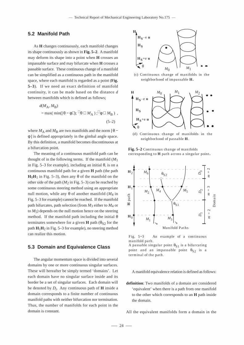
–– Technical Report of Mechanical Engineering Laboratory No.175 ––
––– 24 –––
5.2 Manifold Path
As H changes continuously, each manifold changes
its shape continuously as shown in Fig. 5–2. A manifold
may deform its shape into a point when H crosses animpassable surface and may bifurcate when H crosses a
passable surface. These continuous change of a manifold
can be simplified as a continuous path in the manifoldspace, where each manifold is regarded as a point (Fig.5–3). If we need an exact definition of manifold
continuity, it can be made based on the distance d
between manifolds which is defined as follows;
d(MA, MB)
= max( min(| θ − φ ); ∀θ ∈ MA ) ;∀φ ∈ MB ) ,
(5–2)
where MA and MB are two manifolds and the norm | θ −φ | is defined appropriately in the gimbal angle space.By this definition, a manifold becomes discontinuous at
a bifurcation point.
The meaning of a continuous manifold path can bethought of in the following terms. If the manifold (M1
in Fig. 5–3 for example), including an initial θ, is on a
continuous manifold path for a given H path (the pathH0H1 in Fig. 5–3), then any θ of the manifold on the
other side of the path (M2 in Fig. 5–3) can be reached by
some continuous steering method using an appropriatenull motion, while any θ of another manifold (M4 in
Fig. 5–3 for example) cannot be reached. If the manifold
path bifurcates, path selection (from M3 either to M4 orto M5) depends on the null motion hence on the steering
method. If the manifold path including the initial θterminates somewhere for a given H path (θS2 for thepath H1H2 in Fig. 5–3 for example), no steering method
can realize this motion.
5.3 Domain and Equivalence Class
The angular momentum space is divided into severaldomains by one or more continuous singular surfaces.
These will hereafter be simply termed ‘domains’. Let
each domain have no singular surface inside and itsborder be a set of singular surfaces. Each domain will
be denoted by Di. Any continuous path of H inside a
domain corresponds to a finite number of continuousmanifold paths with neither bifurcation nor termination.
Thus, the number of manifolds for each point in the
domain is constant.
A manifold equivalence relation is defined as follows:
definition : Two manifolds of a domain are considered‘equivalent’ when there is a path from one manifold
to the other which corresponds to an H path inside
the domain.
All the equivalent manifolds form a domain in the
H M0 M1 M2
θ
(d) Continuous change of manifolds in the neighborhood of passable H.
HS+e u
HS–e u
HS
H
M0 M1θ
(c) Continuous change of manifolds in the neighborhood of impassable H.
HS+e u
HS–e u
HS
Fig. 5–2 Continuous change of manifolds corresponding to H path across a singular point.
Fig. 5−3 An example of a continuous manifold path. A passable singular point θS1 is a bifurcating point and an impassable point θS2 is a terminal of the path.
M3M1
M5M4
θS2
θS1
H1
H0
D1
D2
D3
m =
2m
= 3
m =
2
H p
ath
Dom
ain
Manifold Paths
M2
M6H2
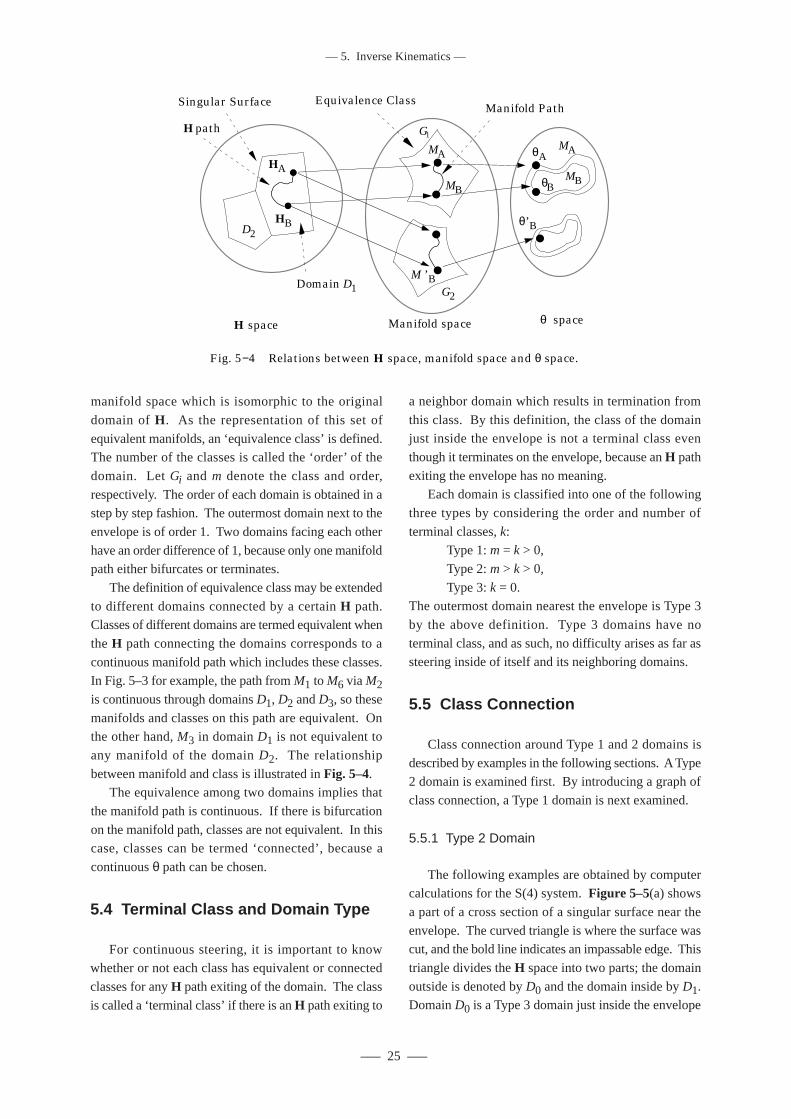
––– 25 –––
–– 5. Inverse Kinematics ––
manifold space which is isomorphic to the original
domain of H . As the representation of this set of
equivalent manifolds, an ‘equivalence class’ is defined.The number of the classes is called the ‘order’ of the
domain. Let Gi and m denote the class and order,
respectively. The order of each domain is obtained in astep by step fashion. The outermost domain next to the
envelope is of order 1. Two domains facing each other
have an order difference of 1, because only one manifoldpath either bifurcates or terminates.
The definition of equivalence class may be extended
to different domains connected by a certain H path.Classes of different domains are termed equivalent when
the H path connecting the domains corresponds to a
continuous manifold path which includes these classes.In Fig. 5–3 for example, the path from M1 to M6 via M2is continuous through domains D1, D2 and D3, so these
manifolds and classes on this path are equivalent. Onthe other hand, M3 in domain D1 is not equivalent to
any manifold of the domain D2. The relationship
between manifold and class is illustrated in Fig. 5–4.The equivalence among two domains implies that
the manifold path is continuous. If there is bifurcation
on the manifold path, classes are not equivalent. In thiscase, classes can be termed ‘connected’, because a
continuous θ path can be chosen.
5.4 Terminal Class and Domain Type
For continuous steering, it is important to knowwhether or not each class has equivalent or connected
classes for any H path exiting of the domain. The class
is called a ‘terminal class’ if there is an H path exiting to
a neighbor domain which results in termination from
this class. By this definition, the class of the domainjust inside the envelope is not a terminal class even
though it terminates on the envelope, because an H path
exiting the envelope has no meaning.Each domain is classified into one of the following
three types by considering the order and number of
terminal classes, k:Type 1: m = k > 0,
Type 2: m > k > 0,
Type 3: k = 0.The outermost domain nearest the envelope is Type 3
by the above definition. Type 3 domains have no
terminal class, and as such, no difficulty arises as far assteering inside of itself and its neighboring domains.
5.5 Class Connection
Class connection around Type 1 and 2 domains is
described by examples in the following sections. A Type2 domain is examined first. By introducing a graph of
class connection, a Type 1 domain is next examined.
5.5.1 Type 2 Domain
The following examples are obtained by computercalculations for the S(4) system. Figure 5–5(a) shows
a part of a cross section of a singular surface near the
envelope. The curved triangle is where the surface wascut, and the bold line indicates an impassable edge. This
triangle divides the H space into two parts; the domain
outside is denoted by D0 and the domain inside by D1.Domain D0 is a Type 3 domain just inside the envelope
Fig. 5−4 Relations between H space, manifold space and θ space.
Domain D1
Equivalence Class
H space Manifold space
HAθB
θ space
H path
MA
G1
G2
HB
MB
θA
θ’B
M ’B
MA
MB
Singular Surface Manifold Path
D2
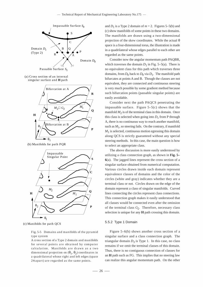
–– Technical Report of Mechanical Engineering Laboratory No.175 ––
––– 26 –––
and D1 is a Type 2 domain of m = 2. Figures 5–5(b) and
(c) show manifolds of some points in these two domains.
The manifolds are drawn using a two-dimensionalprojection of the skew coordinates. While the actual θspace is a four-dimensional torus, the illustration is made
in a quadrilateral whose edges parallel to each other areregarded as the same points.
Consider now the angular momentum path PAQBR,
which traverses the domain D1 in Fig. 5–5(a). There isno equivalent class for this path which traverses three
domains, from D0 back to D0 via D1. The manifold path
bifurcates at points A and B. Though the classes are notequivalent, they are connected and continuous steering
is very much possible by some gradient method because
such bifurcation points (passable singular points) areeasily avoidable.
Consider next the path PAQCS penetrating the
impassable surface. Figure 5–5(c) shows that themanifold M2 is of the terminal class in this domain. Once
this class is selected when going into D1 from P through
A, there is no continuous way to reach another manifold,such as M1, so steering fails. On the contrary, if manifold
M1 is selected, continuous motion egressing this domain
along QCS is strictly guaranteed without any specialsteering methods. In this case, the main question is how
to select an appropriate class.
The above discussion is more easily understood byutilizing a class connection graph, as shown in Fig. 5–6(a). The jagged lines represent the cross section of a
singular surface obtained from numerical computation.Various circles drawn inside each domain represent
equivalence classes of domains and the color of the
circles (white and gray) indicates whether they are aterminal class or not. Circles drawn on the edge of the
domain represent a class of singular manifolds. Curved
lines connecting the circles represent class connections.This connection graph makes it easily understood that
all classes would be connected even after the omission
of the terminal class G2. Therefore, necessary classselection is unique for any H path crossing this domain.
5.5.2 Type 1 Domain
Figure 5–6(b) shows another cross section of a
singular surface and a class connection graph. Thetriangular domain D3 is Type 1. In this case, no class
remains if we omit the terminal classes of this domain.
Thus, there is no contiguous connection of classes foran H path such as FG. This implies that no steering law
can realize this angular momentum path. On the other
(a) Cross section of an internal singular surface and H path
QP
R A
C
S
Impassable Surface S0
Domain D1(Type 2)
Passable Surface S1
B
Domain D0
(c) Manifolds for path QCS
C
Q
S
Impassable Singular Point
M2M1H
θ1
θ2 P
(b) Manifolds for path PQR
P
Q
R
Bifurcation at A
H
θ1
θ2
M2∈ G2M1
Bifurcation at B
Fig. 5-5 Domains and manifolds of the pyramidtype systemA cross section of a Type 2 domain and manifoldsfor several points are obtained by computercalculation. Manifolds are drawn as a twodimensional projection on (θ1, θ2) coordinates ina quadrilateral whose right and left edges (space2π apart) are regarded as the same points.
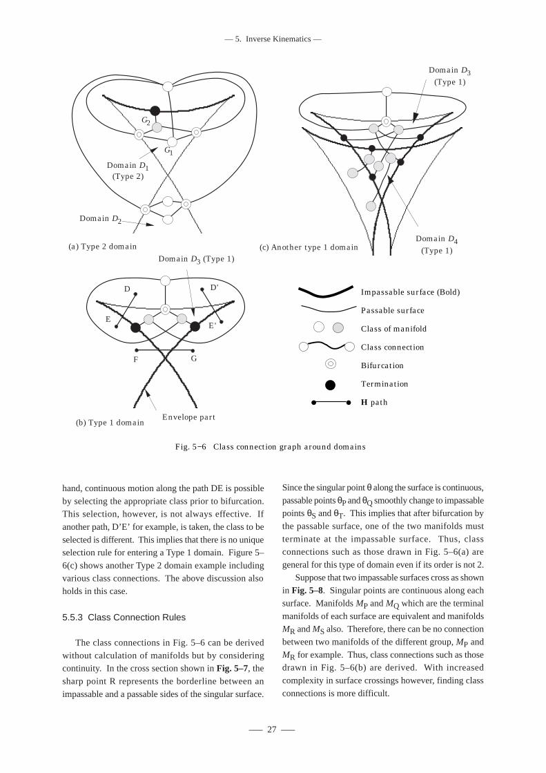
––– 27 –––
–– 5. Inverse Kinematics ––
hand, continuous motion along the path DE is possible
by selecting the appropriate class prior to bifurcation.This selection, however, is not always effective. If
another path, D’E’ for example, is taken, the class to be
selected is different. This implies that there is no uniqueselection rule for entering a Type 1 domain. Figure 5–
6(c) shows another Type 2 domain example including
various class connections. The above discussion alsoholds in this case.
5.5.3 Class Connection Rules
The class connections in Fig. 5–6 can be derived
without calculation of manifolds but by consideringcontinuity. In the cross section shown in Fig. 5–7, the
sharp point R represents the borderline between an
impassable and a passable sides of the singular surface.
Fig. 5−6 Class connection graph around domains
Impassable surface (Bold)
Passable surface
Class of manifold
Class connection
Bifurcation
Termination
H path
Since the singular point θ along the surface is continuous,
passable points θP and θQ smoothly change to impassablepoints θS and θT. This implies that after bifurcation by
the passable surface, one of the two manifolds must
terminate at the impassable surface. Thus, classconnections such as those drawn in Fig. 5–6(a) are
general for this type of domain even if its order is not 2.
Suppose that two impassable surfaces cross as shownin Fig. 5–8. Singular points are continuous along each
surface. Manifolds MP and MQ which are the terminal
manifolds of each surface are equivalent and manifoldsMR and MS also. Therefore, there can be no connection
between two manifolds of the different group, MP and
MR for example. Thus, class connections such as thosedrawn in Fig. 5–6(b) are derived. With increased
complexity in surface crossings however, finding class
connections is more difficult.
(a) Type 2 domain
G1
G2
Domain D1(Type 2)
Domain D2
(b) Type 1 domain
Domain D3 (Type 1)
E
D
GF
Envelope part
E'
D'
(c) Another type 1 domainDomain D4
(Type 1)
Domain D3(Type 1)
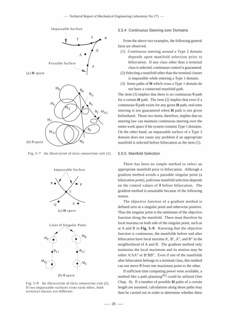
–– Technical Report of Mechanical Engineering Laboratory No.175 ––
––– 28 –––
5.5.4 Continuous Steering over Domains
From the above two examples, the following general
facts are observed.
(1) Continuous steering around a Type 2 domaindepends upon manifold selection prior to
bifurcation. If any class other than a terminal
class is selected, continuous control is guaranteed.(2) Selecting a manifold other than the terminal classes
is impossible while entering a Type 1 domain.
(3) Some paths of H which cross a Type 1 domain donot have a connected manifold path.
The item (3) implies that there is no continuous θ path
for a certain H path. The item (2) implies that even if acontinuous θ path exists for any given H path, real-time
steering is not guaranteed when H path is not given
beforehand. Those two items, therefore, implies that nosteering law can maintain continuous steering over the
entire work space if the system contains Type 1 domains.
On the other hand, an impassable surface of a Type 2domain does not cause any problem if an appropriate
manifold is selected before bifurcation as the item (1).
5.5.5 Manifold Selection
There has been no simple method to select anappropriate manifold prior to bifurcation. Although a
gradient method avoids a passable singular point (a
bifurcation point), judicious manifold selection dependson the control values of θ before bifurcation. The
gradient method is unsuitable because of the following
reason.The objective function of a gradient method is
defined zero at a singular point and otherwise positive.
Thus the singular point is the minimum of the objectivefunction along the manifold. There must therefore be
local maxima on both side of the singular point, such as
at A and B in Fig. 5–9. Knowing that the objectivefunction is continuous, the manifolds before and after
bifurcation have local maxima A’, B’, A”, and B” in the
neighborhood of A and B. The gradient method onlymaintains the local maximum and its motion may be
either A’AA” or B’BB”. Even if one of the manifolds
after bifurcation belongs to a terminal class, this methodcan not move θ from one maximum point to the other.
If sufficient time computing power were available, a
method like a path planning42) could be utilized (SeeChap. 8). If a number of possible H paths of a certain
length are assumed, calculations along those paths may
then be carried out in order to determine whether there
Impassable Surface
Passable SurfaceP
Q
RST
A
(a) H space
Fig. 5−7 An illustration of class connection rule (1).
(b) θ space
MT
MP
MQ
MR
MS
θP
θQ
θR
θS
θT
MA1
MA2
(a) H space
Impassable Surface
P
Q
R
S
T
Fig. 5−8 An illustration of class connection rule (2).If two impassable surfaces cross each other, both terminal classes are different.
(b) θ space
MP
MQ
MR
MS
Lines of Singular Point
θT1 θT2
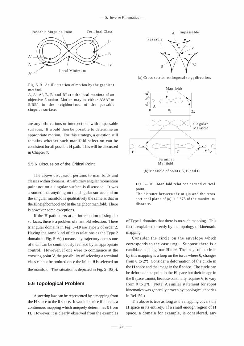
––– 29 –––
–– 5. Inverse Kinematics ––
are any bifurcations or intersections with impassablesurfaces. It would then be possible to determine an
appropriate motion. For this strategy, a question still
remains whether such manifold selection can beconsistent for all possible H path. This will be discussed
in Chapter 7.
5.5.6 Discussion of the Critical Point
The above discussion pertains to manifolds andclasses within domains. An arbitrary angular momentum
point not on a singular surface is discussed. It was
assumed that anything on the singular surface and onthe singular manifold is qualitatively the same as that in
the H neighborhood and in the neighbor manifold. There
is however some exceptions.If the H path starts at an intersection of singular
surfaces, there is a problem of manifold selection. Three
triangular domains in Fig. 5–10 are Type 2 of order 2.Having the same kind of class relations as the Type 2
domain in Fig. 5–6(a) means any trajectory across one
of them can be continuously realized by an appropriatecontrol. However, if one were to commence at the
crossing point V, the possibility of selecting a terminal
class cannot be omitted once the initial θ is selected on
the manifold. This situation is depicted in Fig. 5–10(b).
5.6 Topological Problem
A steering law can be represented by a mapping from
the H space to the θ space. It would be nice if there is a
continuous mapping which uniquely determines θ fromH. However, it is clearly observed from the examples
of Type 1 domains that there is no such mapping. This
fact is explained directly by the topology of kinematicmapping.
Consider the circle on the envelope which
corresponds to the case u=gi . Suppose there is acandidate mapping from H to θ. The image of the circle
by this mapping is a loop on the torus where θi changes
from 0 to 2π. Consider a deformation of the circle inthe H space and the image in the θ space. The circle can
be deformed to a point in the H space but their image in
the θ space cannot, because continuity requires θi to varyfrom 0 to 2π. (Note: A similar statement for robot
kinematics was generally proven by topological theories
in Ref. 59.)The above is true as long as the mapping covers the
H space in its entirety. If a small enough region of Hspace, a domain for example, is considered, any
Passable Singular Point
A
A'
A"
B"
B
B'
Terminal Class
Local Minimum
Fig. 5−9 An illustration of motion by the gradient method.A, A', A", B, B' and B" are the local maxima of an objective function. Motion may be either A'AA" or B'BB" in the neighborhood of the passable singular surface.
Fig. 5–10 Manifold relations around critical point. The distance between the origin and the cross sectional plane of (a) is 0.875 of the maximum distance.
V
A
B C
Impassable
Passable
(a) Cross section orthogonal to gi direction.
(b) Manifold of points A, B and C
V
θ1
θ 2, θ
3, θ
4
Terminal Manifold
A
B C
Manifolds
Singular Manifold
0 2¹
MSV
–– Technical Report of Mechanical Engineering Laboratory No.175 ––
––– 30 –––
continuous steering law can obviously realize such a
continuous mapping. Even if such a region includes a
Type 2 domain, we can realize such a mapping by usingan appropriate manifold selection. Thus, the question is
how large a region of H space can be covered by such a
continuous mapping, and what steering law actually canrealize such a mapping.
It is to be noted that the examples of Type 1 domains
and critical points in the previous section are only foundnear the envelope by various computer calculations of
the S(4) system. Therefore, the above problems may
not be serious. On the other hand, the discussion in this
chapter only suggested that there is a possibility of
continuous steering in the presence of a Type 2 domain.The discussion in the above pertains to the local area
around one domain. In actuality, the candidate
workspace may involve various domains, so a study ofglobal class connections is necessary. In the following
chapters, a relatively specific problem will be studied
for the symmetric pyramid type system using geometrictools given in this chapter.
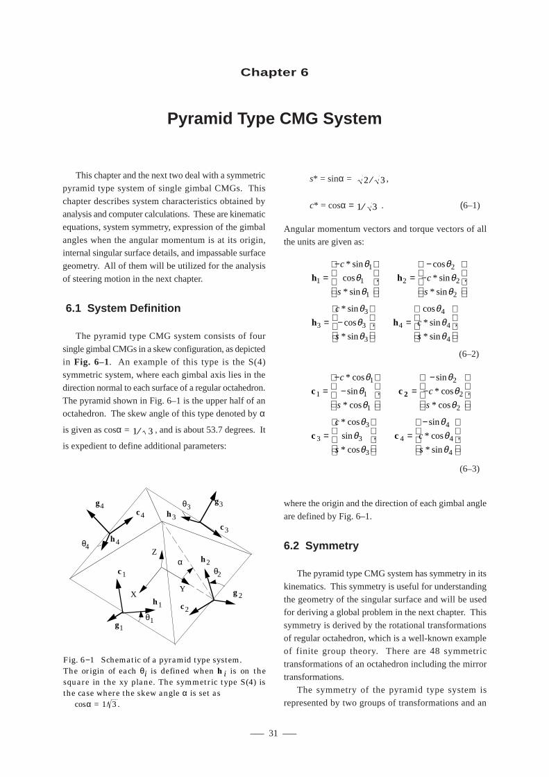
––– 31 –––
–– 6. Pyramid Type CMG System ––
This chapter and the next two deal with a symmetric
pyramid type system of single gimbal CMGs. This
chapter describes system characteristics obtained byanalysis and computer calculations. These are kinematic
equations, system symmetry, expression of the gimbal
angles when the angular momentum is at its origin,internal singular surface details, and impassable surface
geometry. All of them will be utilized for the analysis
of steering motion in the next chapter.
6.1 System Definition
The pyramid type CMG system consists of four
single gimbal CMGs in a skew configuration, as depicted
in Fig. 6–1. An example of this type is the S(4)symmetric system, where each gimbal axis lies in the
direction normal to each surface of a regular octahedron.
The pyramid shown in Fig. 6–1 is the upper half of anoctahedron. The skew angle of this type denoted by α
is given as cosα = 1 3⁄ , and is about 53.7 degrees. It
is expedient to define additional parameters:
s* = sinα = 2 3⁄ ,
c* = cosα = 1 3⁄ . (6–1)
Angular momentum vectors and torque vectors of allthe units are given as:
Chapter 6
Pyramid Type CMG System
c c
c c
21
1
1
1
2
2
2
3
3
3
3
4
4
4
4
=−
−
=−
−
=
=−
c
sc
s
c
scs
* cos
sin
* cos
,
sin
* cos
* cos
,
* cos
sin
* cos
,
sin
* cos
* sin
,
θθθ
θθ
θ
θθ
θ
θθθ
XY
Z
g1
g2
g3g4
h4
θ1
θ4
c1
c4
h1 c2
h2
h3c3
θ2
θ3
α
Fig. 6−1 Schematic of a pyramid type system.The origin of each θi is defined when hi is on thesquare in the xy plane. The symmetric type S(4) isthe case where the skew angle α is set as cosα = . 1/ 3
(6–2)
(6–3)
h h
h h
1
1
1
1
2
2
2
2
3
3
3
3
4
4
4
4
=−
=−
−
= −
=
c
sc
s
c
scs
* sin
cos
* sin
,
cos
* sin
* sin
,
* sin
cos
* sin
,
cos
* sin
* sin
,
θθ
θ
θθ
θ
θθθ
θθθ
where the origin and the direction of each gimbal angle
are defined by Fig. 6–1.
6.2 Symmetry
The pyramid type CMG system has symmetry in its
kinematics. This symmetry is useful for understanding
the geometry of the singular surface and will be usedfor deriving a global problem in the next chapter. This
symmetry is derived by the rotational transformations
of regular octahedron, which is a well-known exampleof finite group theory. There are 48 symmetric
transformations of an octahedron including the mirror
transformations.The symmetry of the pyramid type system is
represented by two groups of transformations and an
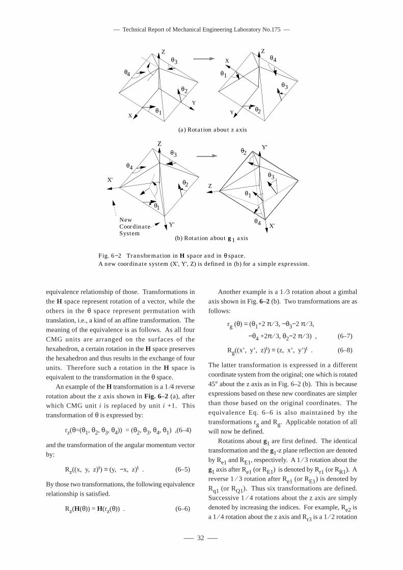
–– Technical Report of Mechanical Engineering Laboratory No.175 ––
––– 32 –––
equivalence relationship of those. Transformations in
the H space represent rotation of a vector, while the
others in the θ space represent permutation withtranslation, i.e., a kind of an affine transformation. The
meaning of the equivalence is as follows. As all four
CMG units are arranged on the surfaces of thehexahedron, a certain rotation in the H space preserves
the hexahedron and thus results in the exchange of four
units. Therefore such a rotation in the H space isequivalent to the transformation in the θ space.
An example of the H transformation is a 1 ⁄4 reverse
rotation about the z axis shown in Fig. 6–2 (a), afterwhich CMG unit i is replaced by unit i +1. This
transformation of θ is expressed by:
rz(θ=(θ1, θ2, θ3, θ4)) = (θ2, θ3, θ4, θ1) ,(6–4)
and the transformation of the angular momentum vectorby:
Rz((x, y, z)t) = (y, −x, z)t . (6–5)
By those two transformations, the following equivalence
relationship is satisfied.
Rz(H(θ)) = H(rz(θ)) . (6–6)
Another example is a 1 ⁄3 rotation about a gimbal
axis shown in Fig. 6–2 (b). Two transformations are as
follows:
rg (θ) = (θ1+2 π ⁄ 3, −θ3−2 π ⁄ 3,
−θ4 +2π ⁄ 3, θ2−2 π ⁄ 3) , (6–7)
Rg((x’, y’, z)t) = (z, x’, y’)t . (6–8)
The latter transformation is expressed in a different
coordinate system from the original; one which is rotated
45° about the z axis as in Fig. 6–2 (b). This is becauseexpressions based on these new coordinates are simpler
than those based on the original coordinates. The
equivalence Eq. 6–6 is also maintained by thetransformations rg and Rg. Applicable notation of all
will now be defined.
Rotations about g1 are first defined. The identicaltransformation and the g1-z plane reflection are denoted
by Re1 and RE1, respectively. A 1 ⁄ 3 rotation about the
g1 axis after Re1 (or RE1) is denoted by Rr1 (or RR1). Areverse 1 ⁄ 3 rotation after Re1 (or RE1) is denoted by
Rq1 (or RQ1). Thus six transformations are defined.
Successive 1 ⁄ 4 rotations about the z axis are simplydenoted by increasing the indices. For example, Re2 is
a 1 ⁄ 4 rotation about the z axis and Rr3 is a 1 ⁄ 2 rotation
Z
(a) Rotation about z axis
Z
θ1
θ4
θ2
θ3
X
YX
Z
θ1
θ4
θ2
θ3
Y
(b) Rotation about g1 axis
Y'
X'
θ1
θ4
θ2
θ3
New Coordinate System
X'
Zθ1
θ4
θ2
θ3
Y'
Fig. 6−2 Transformation in H space and in θ space. A new coordinate system (X', Y', Z) is defined in (b) for a simple expression.
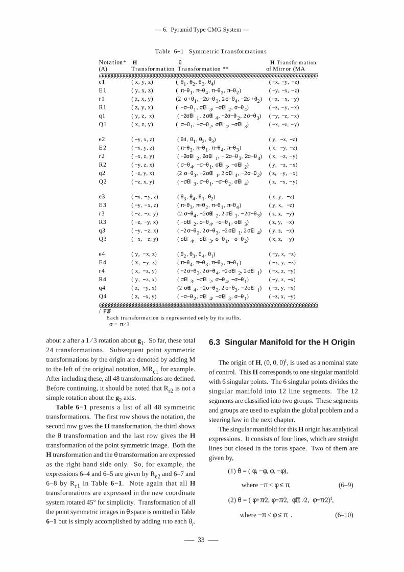
––– 33 –––
–– 6. Pyramid Type CMG System ––
6.3 Singular Manifold for the H Origin
The origin of H, (0, 0, 0)t, is used as a nominal state
of control. This H corresponds to one singular manifold
with 6 singular points. The 6 singular points divides thesingular manifold into 12 line segments. The 12
segments are classified into two groups. These segments
and groups are used to explain the global problem and asteering law in the next chapter.
The singular manifold for this H origin has analytical
expressions. It consists of four lines, which are straightlines but closed in the torus space. Two of them are
given by,
(1) θ = ( φ, −φ, φ, −φ),
where −π < φ ≤ π, (6–9)
(2) θ = ( φ+π⁄2, φ−π⁄2, φ+π⁄2, φ−π⁄2)t,
where −π < φ ≤ π . (6–10)
Table 6−1 Symmetric Transformations
Notation* H θ H Transformation (A) Transformation Transformation ** of Mirror (MA )_________________________________________________________________________e1 ( x, y, z) ( θ1, θ2, θ3, θ4) ( −x, −y, −z)
E1 ( y, x, z) ( π−θ1, π−θ4, π−θ3, π−θ2) ( −y, −x, −z)
r1 ( z, x, y) (2 σ+θ1, −2σ−θ3, 2σ−θ4, −2σ+θ2) ( −z, −x, −y)
R1 ( z, y, x) ( −σ−θ1, σ+θ3, −σ+θ2, σ−θ4) ( −z, −y, −x)
q1 ( y, z, x) ( −2σ+θ1, 2σ+θ4, −2σ−θ2, 2σ−θ3) ( −y, −z, −x)
Q1 ( x, z, y) ( σ−θ1, −σ−θ2, σ+θ4, −σ+θ3) ( −x, −z, −y)
e2 ( −y, x, z) ( θ4, θ1, θ2, θ3) ( y, −x, −z)
E2 ( −x, y, z) ( π−θ2, π−θ1, π−θ4, π−θ3) ( x, −y, −z)
r2 ( −x, z, y) ( −2σ+θ2, 2σ+θ1, − 2σ−θ3, 2σ−θ4) ( x, −z, −y)
R2 ( −y, z, x) ( σ−θ4, −σ−θ1, σ+θ3, −σ+θ2) ( y, −z, −x)
q2 ( −z, y, x) (2 σ−θ3, −2σ+θ1, 2 σ+θ4, −2σ−θ2) ( z, −y, −x)
Q2 ( −z, x, y) ( −σ+θ3, σ−θ1, −σ−θ2, σ+θ4) ( z, −x, −y)
e3 ( −x, −y, z) ( θ3, θ4, θ1, θ2) ( x, y, −z)
E3 ( −y, −x, z) ( π−θ3, π−θ2, π−θ1, π−θ4) ( y, x, −z)
r3 ( −z, −x, y) (2 σ−θ4, −2σ+θ2, 2 σ+θ1, −2σ−θ3) ( z, x, −y)
R3 ( −z, −y, x) ( −σ+θ2, σ−θ4, −σ−θ1, σ+θ3) ( z, y, −x)
q3 ( −y, −z, x) ( −2σ−θ2, 2σ−θ3, −2σ+θ1, 2σ+θ4) ( y, z, −x)
Q3 ( −x, −z, y) ( σ+θ4, −σ+θ3, σ−θ1, −σ−θ2) ( x, z, −y)
e4 ( y, −x, z) ( θ2, θ3, θ4, θ1) ( −y, x, −z)
E4 ( x, −y, z) ( π−θ4, π−θ3, π−θ2, π−θ1) ( −x, y, −z)
r4 ( x, −z, y) ( −2σ−θ3, 2σ−θ4, −2σ+θ2, 2σ+θ1) ( −x, z, −y)
R4 ( y, −z, x) ( σ+θ3, −σ+θ2, σ−θ4, −σ−θ1) ( −y, z, −x)
q4 ( z, −y, x) (2 σ+θ4, −2σ−θ2, 2 σ−θ3, −2σ+θ1) ( −z, y, −x)
Q4 ( z, −x, y) ( −σ−θ2, σ+θ4, −σ+θ3, σ−θ1) ( −z, x, −y)
_________________________________________________________________________Note; *: Each transformation is represented only by its suffix. **: σ = π ⁄ 3
about z after a 1 ⁄ 3 rotation about g1. So far, these total
24 transformations. Subsequent point symmetric
transformations by the origin are denoted by adding Mto the left of the original notation, MRe1 for example.
After including these, all 48 transformations are defined.
Before continuing, it should be noted that Rr2 is not asimple rotation about the g2 axis.
Table 6−1 presents a list of all 48 symmetric
transformations. The first row shows the notation, thesecond row gives the H transformation, the third shows
the θ transformation and the last row gives the Htransformation of the point symmetric image. Both theH transformation and the θ transformation are expressed
as the right hand side only. So, for example, the
expressions 6–4 and 6–5 are given by Re2 and 6–7 and6–8 by Rr1 in Table 6−1. Note again that all Htransformations are expressed in the new coordinate
system rotated 45° for simplicity. Τransformation of allthe point symmetric images in θ space is omitted in Table
6−1 but is simply accomplished by adding π to each θi.
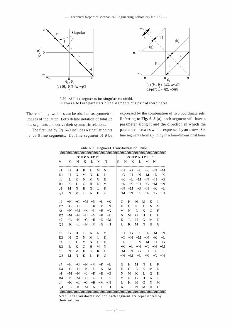
–– Technical Report of Mechanical Engineering Laboratory No.175 ––
––– 34 –––
Table 6−2 Segment Transformation Rule_____________________________________________________________ Transformation A Transformation MAΑ G H K L M N G H K L M N--------------------------------------------------------------------------------------------e1 G H K L M N −H −G −L −K −N −ME1 H G M N K L −G −H −N −M −L −Kr1 L K N M G H −K −L −M −N −H −GR1 K L G H N M −L −K −H −G −M −Nq1 M N H G L K −N −M −G −H −K −LQ1 N M L K H G −M −N −K −L −G −H
e2 −H −G −M −N −L −K G H N M K LE2 −G −H −L −K −M −N H G K L N Mr2 −N −M −Κ −L −H −G M N L K G HR2 −M −N −H −G −K −L N M G H L Hq2 −L −K −G −H −N −M K L H G M NQ2 −K −L −N −M −G −H L K M N H G
e3 G H L K N M −H −G −K −L −M −NE3 H G N M L K −G −H −M −N −K −Lr3 K L M N G H −L −K −N −M −H −GR3 L K G H M N −K −L −H −G −N −Mq3 N M H G K L −M −N −G −H −L −KQ3 M N K L H G −N −M −L −K −G −H
e4 −H −G −N −M −K −L G H M N L KE4 −G −H −K −L −N −M H G L K M Nr4 −M −N −L −K −H −G N M K L G HR4 −N −M −H −G −L −K M N G H K Lq4 −K −L −G −H −M −N L K H G N MQ4 −L −K −M −N −G −H K L N M H G_____________________________________________________________Note:Each transformation and each segment are represented by their suffices.
The remaining two lines can be obtained as symmetric
images of the latter. Let’s define notation of total 12
line segments and derive their symmetric relations.The first line by Eq. 6–9 includes 6 singular points
hence 6 line segments. Let line segment of θ be
expressed by the combination of two coordinate sets.
Referring to Fig. 6–3 (a), each segment will have aparameter along it and the direction in which the
parameter increases will be expressed by an arrow. Six
line segments from LA to LF in a four-dimensional torus
(b) (θi, θj)=(φ+ψ, φ−ψ) 0≤φ≤π, ψ= π⁄2, –5π⁄6
0 π−π θi
0
π
−π
θ j
g
(g)
(h)
h
k
l
(k)
(l)
Fig. 6−3 Line segments for singular manifold.Arrows a to l are parametric line segments of a pair of coordinates.
(a) (θi, θj) =(φ, −φ)
0 π−πθ1, θ3
0
π
−π
θ 2, θ
4 a
d
c
b
e
f
Singular
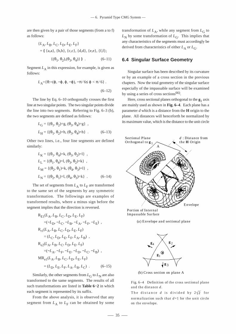
––– 35 –––
–– 6. Pyramid Type CMG System ––
are then given by a pair of those segments (from a to f)
as follows:
{ LA, LB, LC, LD, LE, LF}
= { {a,a}, {b,b}, {c,c}, {d,d}, {e,e}, {f,f};
{(θ1, θ2),(θ3, θ4)} } . (6–11)
Segment LA in this expression, for example, is given asfollows:
LA={θ:=(ϕ, −ϕ, ϕ, −ϕ), −π ⁄ 6≤ ϕ < π ⁄ 6} .
(6–12)
The line by Eq. 6–10 orthogonally crosses the first
line at two singular points. The two singular points dividethe line into two segments. Referring to Fig. 6–3 (b),
the two segments are defined as follows:
LG = {(θ1, θ2)=g, (θ3, θ4)=g} ,
LH = {(θ1, θ2)=h, (θ3, θ4)=h} . (6–13)
Other two lines, i.e., four line segments are definedsimilarly:
LK = {(θ1, θ4)=k, (θ3, θ2)=l} ,
LL = {(θ1, θ4)=l, (θ3, θ2)=k} ,
LM = {(θ2, θ1)=k, (θ4, θ3)=l} ,
LN = {(θ2, θ1)=l, (θ4, θ3)=k} . (6–14)
The set of segments from LA to LF are transformed
to the same set of the segments by any symmetrictransformation. The followings are examples of
transformed results, where a minus sign before the
segment implies that the direction is reversed.
RE1(LA, LB, LC, LD, LE, LF)
=(−LD, −LC, −LB, −LA, −LF, −LE) ,
Rr1(LA, LB, LC, LD, LE, LF)
= (LC, LD, LE, LF, LA, LB) ,
Re2(LA, LB, LC, LD, LE, LF)
=(−LA, −LF, −LE, −LD, −LC, −LB) ,
MRe1(LA, LB, LC, LD, LE, LF)
= (LD, LE, LF, LA, LB, LC) . (6–15)
Similarly, the other segments from LG to LN are also
transformed to the same segments. The results of all
such transformations are listed in Table 6−2 in whicheach segment is represented by its suffix.
From the above analysis, it is observed that any
segment from LA to LF can be obtained by some
transformation of LA, while any segment from LG to
LN by some transformation of LG. This implies that
any characteristics of the segments must accordingly bederived from characteristics of either LA or LG.
6.4 Singular Surface Geometry
Singular surface has been described by its curvature
or by an example of a cross section in the previouschapters. Now the total geometry of the singular surface
especially of the impassable surface will be examined
by using a series of cross sections66).Here, cross sectional planes orthogonal to the g1 axis
are mainly used as shown in Fig. 6–4. Each plane has a
parameter d which is a distance from the H origin to theplane. All distances will henceforth be normalized by
its maximum value, which is the distance to the unit circle
g1
g4g2
g3
Sectional Plane Orthogonal to g1
d : Distance from the H Origin
Portion of Internal Impassable Surface
Envelope
(a) Envelope and sectional plane
(b) Cross section on plane A
A
Fig. 6–4 Definition of the cross sectional planeand the distance d.
The distance d i s d ivided by 2 2 for
normalization such that d=1 for the unit circleon the envelope.
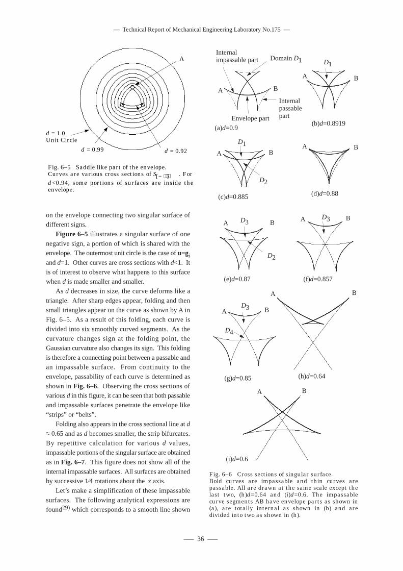
–– Technical Report of Mechanical Engineering Laboratory No.175 ––
––– 36 –––
Fig. 6–5 Saddle like part of the envelope.Curves are various cross sections of S{− + + +} . For d<0.94, some portions of surfaces are inside theenvelope.
d = 1.0Unit Circle
d = 0.99 d = 0.92
A
on the envelope connecting two singular surface ofdifferent signs.
Figure 6–5 illustrates a singular surface of one
negative sign, a portion of which is shared with theenvelope. The outermost unit circle is the case of u=giand d=1. Other curves are cross sections with d<1. It
is of interest to observe what happens to this surfacewhen d is made smaller and smaller.
As d decreases in size, the curve deforms like a
triangle. After sharp edges appear, folding and thensmall triangles appear on the curve as shown by A in
Fig. 6–5. As a result of this folding, each curve is
divided into six smoothly curved segments. As thecurvature changes sign at the folding point, the
Gaussian curvature also changes its sign. This folding
is therefore a connecting point between a passable andan impassable surface. From continuity to the
envelope, passability of each curve is determined as
shown in Fig. 6–6. Observing the cross sections ofvarious d in this figure, it can be seen that both passable
and impassable surfaces penetrate the envelope like
“strips” or “belts”.Folding also appears in the cross sectional line at d
≈ 0.65 and as d becomes smaller, the strip bifurcates.
By repetitive calculation for various d values,impassable portions of the singular surface are obtained
as in Fig. 6–7. This figure does not show all of the
internal impassable surfaces. All surfaces are obtainedby successive 1⁄4 rotations about the z axis.
Let’s make a simplification of these impassable
surfaces. The following analytical expressions arefound29) which corresponds to a smooth line shown
Fig. 6–6 Cross sections of singular surface.Bold curves are impassable and thin curves are passable. All are drawn at the same scale except the last two, (h)d=0.64 and (i)d=0.6. The impassable curve segments AB have envelope parts as shown in (a), are totally internal as shown in (b) and are divided into two as shown in (h).
Internal impassable part
Internal passable partEnvelope part
Domain D1
(a)d=0.9
A B
(c)d=0.885 (d)d=0.88
A
(e)d=0.87
D3
(f)d=0.857
A
(b)d=0.8919
A
D1
B
B
B
A B
(i)d=0.6
A B
D2
A
D1B
D3A
D2
B
D4
(g)d=0.85
AD3 B
(h)d=0.64
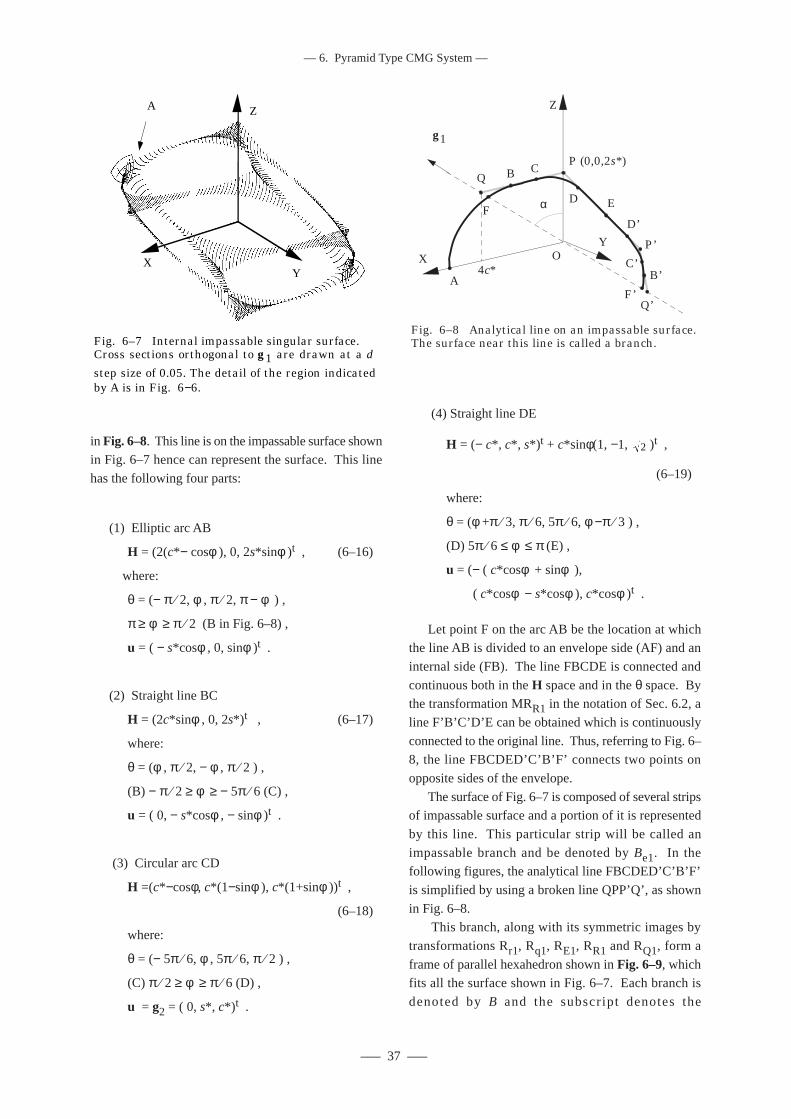
––– 37 –––
–– 6. Pyramid Type CMG System ––
in Fig. 6–8. This line is on the impassable surface shownin Fig. 6–7 hence can represent the surface. This line
has the following four parts:
(1) Elliptic arc AB
H = (2(c*− cosφ ), 0, 2s*sinφ )t , (6–16)
where:
θ = (− π ⁄ 2, φ , π ⁄ 2, π − φ ) ,
π ≥ φ ≥ π ⁄ 2 (B in Fig. 6–8) ,
u = ( − s*cosφ , 0, sinφ )t .
(2) Straight line BC
H = (2c*sinφ , 0, 2s*) t , (6–17)
where:
θ = (φ , π ⁄ 2, − φ , π ⁄ 2 ) ,
(B) − π ⁄ 2 ≥ φ ≥ − 5π ⁄ 6 (C) ,
u = ( 0, − s*cosφ , − sinφ )t .
(3) Circular arc CD
H =(c*−cosφ, c*(1−sinφ ), c*(1+sinφ ))t ,
(6–18)
where:
θ = (− 5π ⁄ 6, φ , 5π ⁄ 6, π ⁄ 2 ) ,
(C) π ⁄ 2 ≥ φ ≥ π ⁄ 6 (D) ,
u = g2 = ( 0, s*, c*) t .
(4) Straight line DE
H = (− c*, c*, s*) t + c*sinφ(1, −1, 2 )t ,
(6–19)
where:
θ = (φ +π ⁄ 3, π ⁄ 6, 5π ⁄ 6, φ −π ⁄ 3 ) ,
(D) 5π ⁄ 6 ≤ φ ≤ π (E) ,
u = (− ( c*cosφ + sinφ ),
( c*cosφ − s*cosφ ), c*cosφ )t .
Let point F on the arc AB be the location at whichthe line AB is divided to an envelope side (AF) and an
internal side (FB). The line FBCDE is connected and
continuous both in the H space and in the θ space. Bythe transformation MRR1 in the notation of Sec. 6.2, a
line F’B’C’D’E can be obtained which is continuously
connected to the original line. Thus, referring to Fig. 6–8, the line FBCDED’C’B’F’ connects two points on
opposite sides of the envelope.
The surface of Fig. 6–7 is composed of several stripsof impassable surface and a portion of it is represented
by this line. This particular strip will be called an
impassable branch and be denoted by Be1. In thefollowing figures, the analytical line FBCDED’C’B’F’
is simplified by using a broken line QPP’Q’, as shown
in Fig. 6–8. This branch, along with its symmetric images by
transformations Rr1, Rq1, RE1, RR1 and RQ1, form a
frame of parallel hexahedron shown in Fig. 6–9, whichfits all the surface shown in Fig. 6–7. Each branch is
denoted by B and the subscript denotes the
Fig. 6–7 Internal impassable singular surface.Cross sections orthogonal to g1 are drawn at a d
step size of 0.05. The detail of the region indicated by A is in Fig. 6−6.
XY
ZA
Fig. 6–8 Analytical line on an impassable surface.The surface near this line is called a branch.
XY
Z
g1
QP (0,0,2s*)
E
A
B C
D
P’
D’
C’B’
Q’
F
F’
O
α
4c*
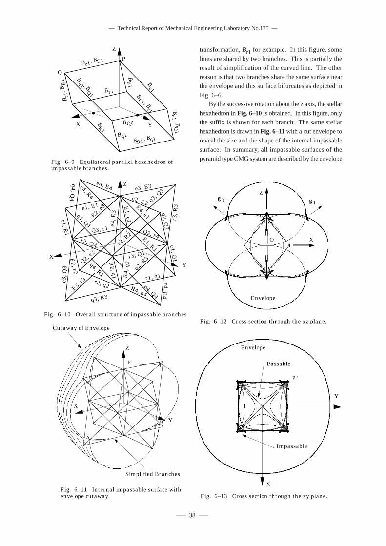
–– Technical Report of Mechanical Engineering Laboratory No.175 ––
––– 38 –––
transformation, Br1 for example. In this figure, some
lines are shared by two branches. This is partially the
result of simplification of the curved line. The otherreason is that two branches share the same surface near
the envelope and this surface bifurcates as depicted in
Fig. 6–6.By the successive rotation about the z axis, the stellar
hexahedron in Fig. 6–10 is obtained. In this figure, only
the suffix is shown for each branch. The same stellarhexahedron is drawn in Fig. 6–11 with a cut envelope to
reveal the size and the shape of the internal impassable
surface. In summary, all impassable surfaces of thepyramid type CMG system are described by the envelope
X
Be1, BE1
Be1
Bq1 , B
Q1
Br1
, BR
1
BE
1
B r1
BR1
Bq1BR1, Bq1
B Q0
Be1 , B
Q1
BE1 , B
r1
Y
Z
Q
P
Fig. 6–9 Equilateral parallel hexahedron of impassable branches.
X
Y
Z
P
Cutaway of Envelope
Simplified Branches
Fig. 6–11 Internal impassable surface with envelope cutaway.
X
Z
O
g1g3
Envelope
Fig. 6–12 Cross section through the xz plane.
Fig. 6–13 Cross section through the xy plane.
P’
X
Y
Envelope
Impassable
Passable
X
r1, R1
e1, E1
q4, Q4
e4, E4r4, R4
Q3, r1
E2, e3
e3, E3
q3, Q3
r3, R
3
e2, E2E4, e1
r2, R
2Q2, r4
q2, Q2
E1, e2
r3, Q1
e1, Q1
E1, R1
r1, q1
r4, E4
e4, Q4R4, q4
q2, R
3
q3, R3
e3, Q
3
E3, r3 r2, q2
E2, r2
R2, q1
q4, R1 R4,
q3
r2, Q4
q1, Q1 e4, E
3
Y
Z
Fig. 6–10 Overall structure of impassable branches
Q2, e2

––– 39 –––
–– 6. Pyramid Type CMG System ––
and the frame like structure of the branches.
Figures 6–12 and 6–13 are examples of other cross
sections which are not orthogonal to the gimbal axes.In these figures, all singular surface, passable and
impassable, are drawn. Two figures show that there are
relatively large region with no singular surface andimpassable surfaces are narrow strips compared with the
maximum workspace. Nevertheless, impassable
surfaces cannot be ignored because they surround the
origin which is the nominal point for the control.
Moreover, some of the impassable surfaces crosses zaxis and others lie on the x-y plane. As the CMG
system’s axes coincide with those of an attitude control
system, angular momentum of the CMG system tend totravel near such axes.

–– Technical Report of Mechanical Engineering Laboratory No.175 ––
––– 40 –––
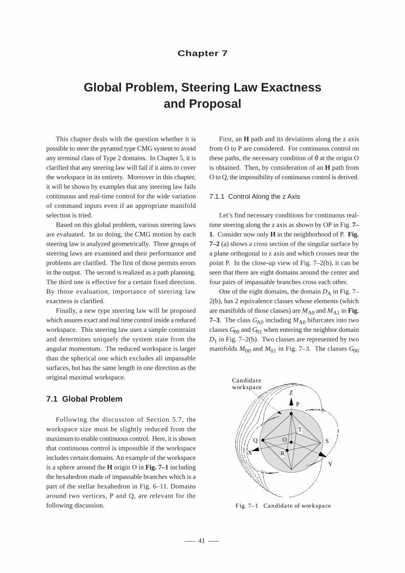
––– 41 –––
–– 7. Global Problem, Steering Law Exactness and Proposal ––
This chapter deals with the question whether it ispossible to steer the pyramid type CMG system to avoid
any terminal class of Type 2 domains. In Chapter 5, it is
clarified that any steering law will fail if it aims to coverthe workspace in its entirety. Moreover in this chapter,
it will be shown by examples that any steering law fails
continuous and real-time control for the wide variationof command inputs even if an appropriate manifold
selection is tried.
Based on this global problem, various steering lawsare evaluated. In so doing, the CMG motion by each
steering law is analyzed geometrically. Three groups of
steering laws are examined and their performance andproblems are clarified. The first of those permits errors
in the output. The second is realized as a path planning.
The third one is effective for a certain fixed direction.By those evaluation, importance of steering law
exactness is clarified.
Finally, a new type steering law will be proposedwhich assures exact and real time control inside a reduced
workspace. This steering law uses a simple constraint
and determines uniquely the system state from theangular momentum. The reduced workspace is larger
than the spherical one which excludes all impassable
surfaces, but has the same length in one direction as theoriginal maximal workspace.
7.1 Global Problem
Following the discussion of Section 5.7, the
workspace size must be slightly reduced from themaximum to enable continuous control. Here, it is shown
that continuous control is impossible if the workspace
includes certain domains. An example of the workspaceis a sphere around the H origin O in Fig. 7–1 including
the hexahedron made of impassable branches which is a
part of the stellar hexahedron in Fig. 6–11. Domainsaround two vertices, P and Q, are relevant for the
following discussion.
Chapter 7
Global Problem, Steering Law Exactnessand Proposal
First, an H path and its deviations along the z axisfrom O to P are considered. For continuous control on
these paths, the necessary condition of θ at the origin O
is obtained. Then, by consideration of an H path fromO to Q, the impossibility of continuous control is derived.
7.1.1 Control Along the z Axis
Let’s find necessary conditions for continuous real-
time steering along the z axis as shown by OP in Fig. 7–1. Consider now only H in the neighborhood of P. Fig.7–2 (a) shows a cross section of the singular surface by
a plane orthogonal to z axis and which crosses near thepoint P. In the close-up view of Fig. 7–2(b), it can be
seen that there are eight domains around the center and
four pairs of impassable branches cross each other.One of the eight domains, the domain DA in Fig. 7–
2(b), has 2 equivalence classes whose elements (which
are manifolds of those classes) are MA0 and MA1 in Fig.7–3. The class GA0 including MA0 bifurcates into two
classes G00 and G01 when entering the neighbor domain
D1 in Fig. 7–2(b). Two classes are represented by twomanifolds M00 and M01 in Fig. 7–3. The classes G00
Fig. 7–1 Candidate of workspace
X
Y
Z
P
R
Q O
Candidate workspace
S
T
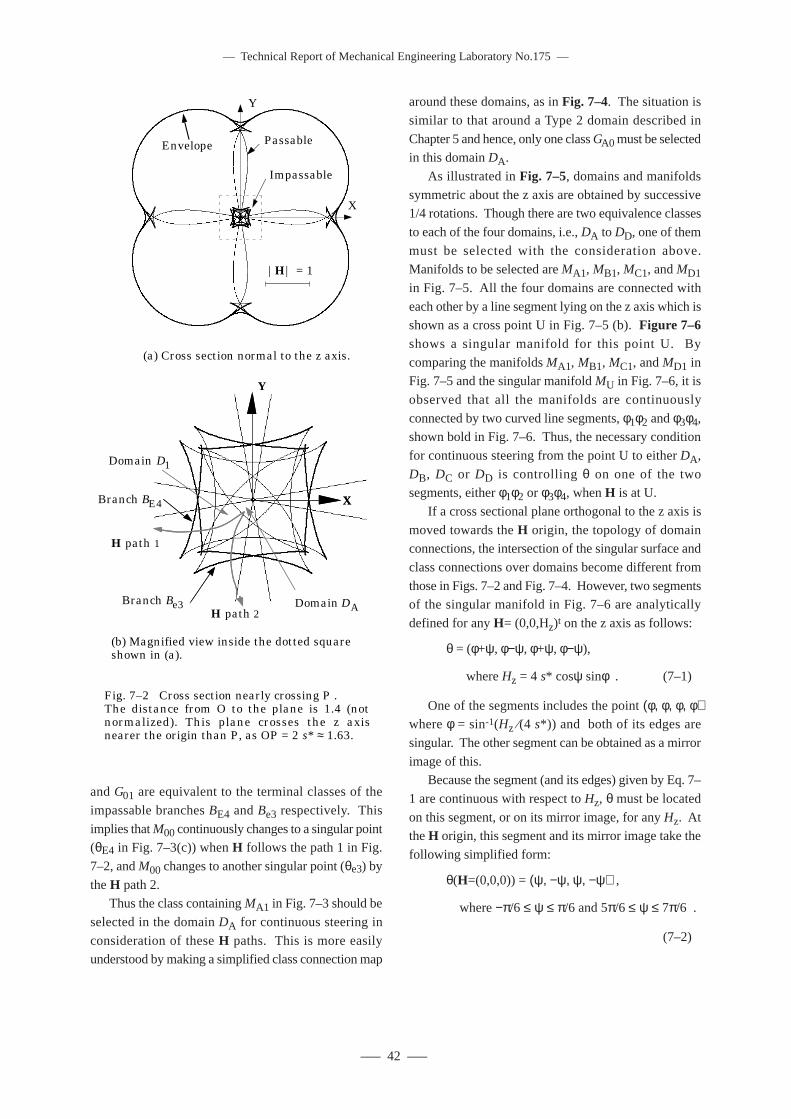
–– Technical Report of Mechanical Engineering Laboratory No.175 ––
––– 42 –––
X
Y
Domain D1
Branch Be3H path 2
(a) Cross section normal to the z axis.
|H| = 1
X
Y
Envelope Passable
Impassable
Domain DA
X
Y
H path 1
Branch BE4
H path 2
(b) Magnified view inside the dotted square shown in (a).
and G01 are equivalent to the terminal classes of the
impassable branches BE4 and Be3 respectively. This
implies that M00 continuously changes to a singular point(θE4 in Fig. 7–3(c)) when H follows the path 1 in Fig.
7–2, and M00 changes to another singular point (θe3) by
the H path 2.Thus the class containing MA1 in Fig. 7–3 should be
selected in the domain DA for continuous steering in
consideration of these H paths. This is more easilyunderstood by making a simplified class connection map
around these domains, as in Fig. 7–4. The situation is
similar to that around a Type 2 domain described in
Chapter 5 and hence, only one class GA0 must be selectedin this domain DA.
As illustrated in Fig. 7–5, domains and manifolds
symmetric about the z axis are obtained by successive1/4 rotations. Though there are two equivalence classes
to each of the four domains, i.e., DA to DD, one of them
must be selected with the consideration above.Manifolds to be selected are MA1, MB1, MC1, and MD1in Fig. 7–5. All the four domains are connected with
each other by a line segment lying on the z axis which isshown as a cross point U in Fig. 7–5 (b). Figure 7–6shows a singular manifold for this point U. By
comparing the manifolds MA1, MB1, MC1, and MD1 inFig. 7–5 and the singular manifold MU in Fig. 7–6, it is
observed that all the manifolds are continuously
connected by two curved line segments, φ1φ2 and φ3φ4,shown bold in Fig. 7–6. Thus, the necessary condition
for continuous steering from the point U to either DA,
DB, DC or DD is controlling θ on one of the twosegments, either φ1φ2 or φ3φ4, when H is at U.
If a cross sectional plane orthogonal to the z axis is
moved towards the H origin, the topology of domainconnections, the intersection of the singular surface and
class connections over domains become different from
those in Figs. 7–2 and Fig. 7–4. However, two segmentsof the singular manifold in Fig. 7–6 are analytically
defined for any H= (0,0,Hz)t on the z axis as follows:
θ = (φ+ψ, φ−ψ, φ+ψ, φ−ψ),
where Hz = 4 s* cosψ sinφ . (7–1)
One of the segments includes the point (φ, φ, φ, φ)where φ = sin-1(Hz ⁄(4 s*)) and both of its edges are
singular. The other segment can be obtained as a mirror
image of this.Because the segment (and its edges) given by Eq. 7–
1 are continuous with respect to Hz, θ must be located
on this segment, or on its mirror image, for any Hz. Atthe H origin, this segment and its mirror image take the
following simplified form:
θ(H=(0,0,0)) = (ψ, −ψ, ψ, −ψ) ,
where −π/6 ≤ ψ ≤ π/6 and 5π/6 ≤ ψ ≤ 7π/6 .
(7–2)
Fig. 7–2 Cross section nearly crossing P .The distance from O to the plane is 1.4 (notnormalized). This plane crosses the z axisnearer the origin than P, as OP = 2 s* ≈ 1.63.
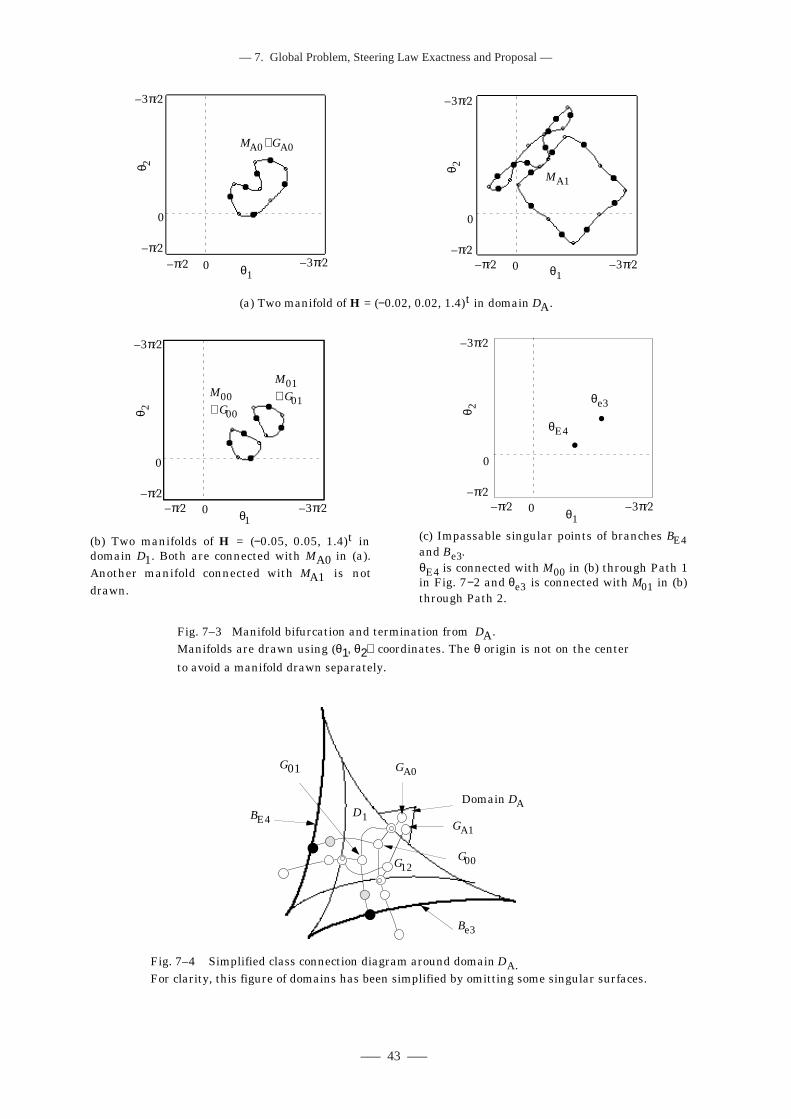
––– 43 –––
–– 7. Global Problem, Steering Law Exactness and Proposal ––
0–π⁄2 –3π⁄2
–3π⁄2
–π⁄2
0
θ1
θ 2MA0 ∈ GA0
MA1
0–π⁄2 –3π⁄2
–3π⁄2
–π⁄2
0
θ1
θ 2
(a) Two manifold of H = (−0.02, 0.02, 1.4)t in domain DA.
Fig. 7–3 Manifold bifurcation and termination from DA.Manifolds are drawn using (θ1, θ2) coordinates. The θ origin is not on the center
to avoid a manifold drawn separately.
(b) Two manifolds of H = (−0.05, 0.05, 1.4)t in domain D1. Both are connected with MA0 in (a).Another manifold connected with MA1 is notdrawn.
M01∈ G01
M00∈ G00
0–π⁄2 –3π⁄2
–3π⁄2
–π⁄2
0
θ1
θ 2
(c) Impassable singular points of branches BE4 and Be3.θE4 is connected with M00 in (b) through Path 1 in Fig. 7−2 and θe3 is connected with M01 in (b) through Path 2.
θE4
θe3
0–π⁄2 –3π⁄2
–3π⁄2
–π⁄2
0
θ1
θ 2
Fig. 7–4 Simplified class connection diagram around domain DA.For clarity, this figure of domains has been simplified by omitting some singular surfaces.
Be3
BE4
Domain DA
GA0
G00
G01
GA1
G12
D1
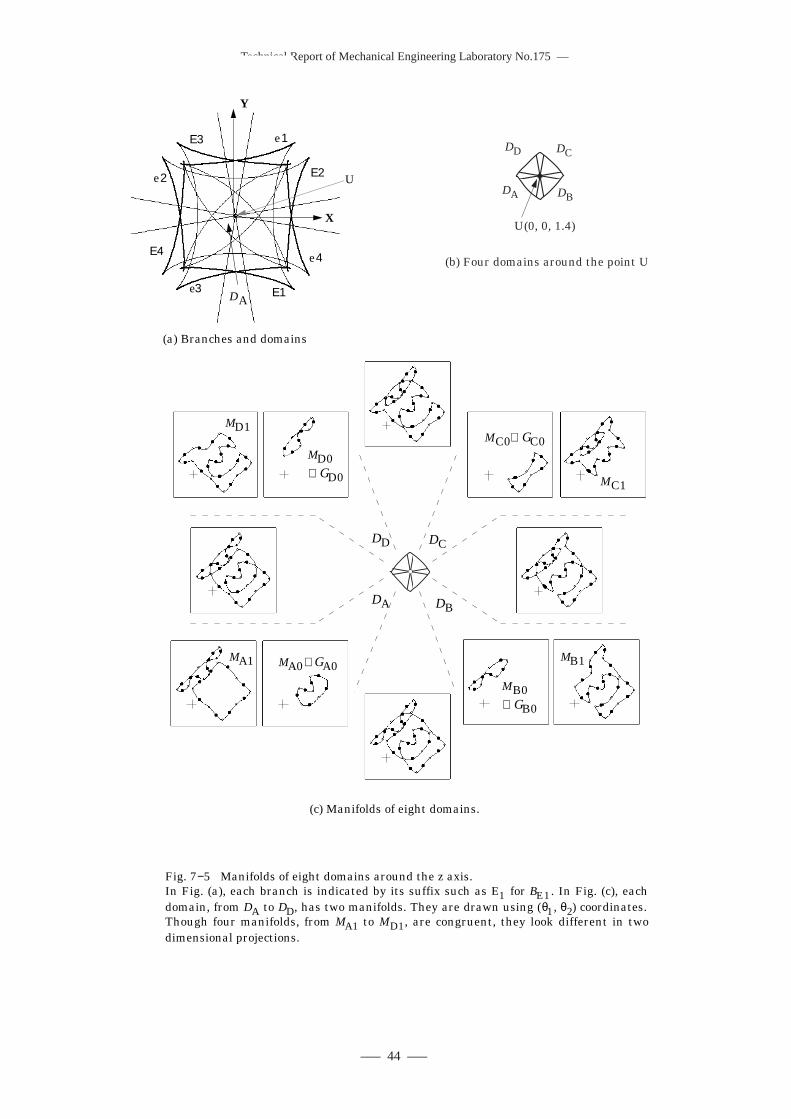
–– Technical Report of Mechanical Engineering Laboratory No.175 ––
––– 44 –––
DC
U(0, 0, 1.4)
DD
DA DB
(b) Four domains around the point U
MC0∈ GC0
MB0∈ GB0
MA0∈ GA0
MD0∈ GD0
DCDD
DA DB
MD1
MA1 MB1
MC1
Fig. 7−5 Manifolds of eight domains around the z axis.In Fig. (a), each branch is indicated by its suffix such as E1 for BE1. In Fig. (c), eachdomain, from DA to DD, has two manifolds. They are drawn using (θ1, θ2) coordinates.Though four manifolds, from MA1 to MD1, are congruent, they look different in twodimensional projections.
(c) Manifolds of eight domains.
X
Y
DA
Ε4
e3 Ε1
Ε2
Ε3
e4
e1
e2 U
(a) Branches and domains
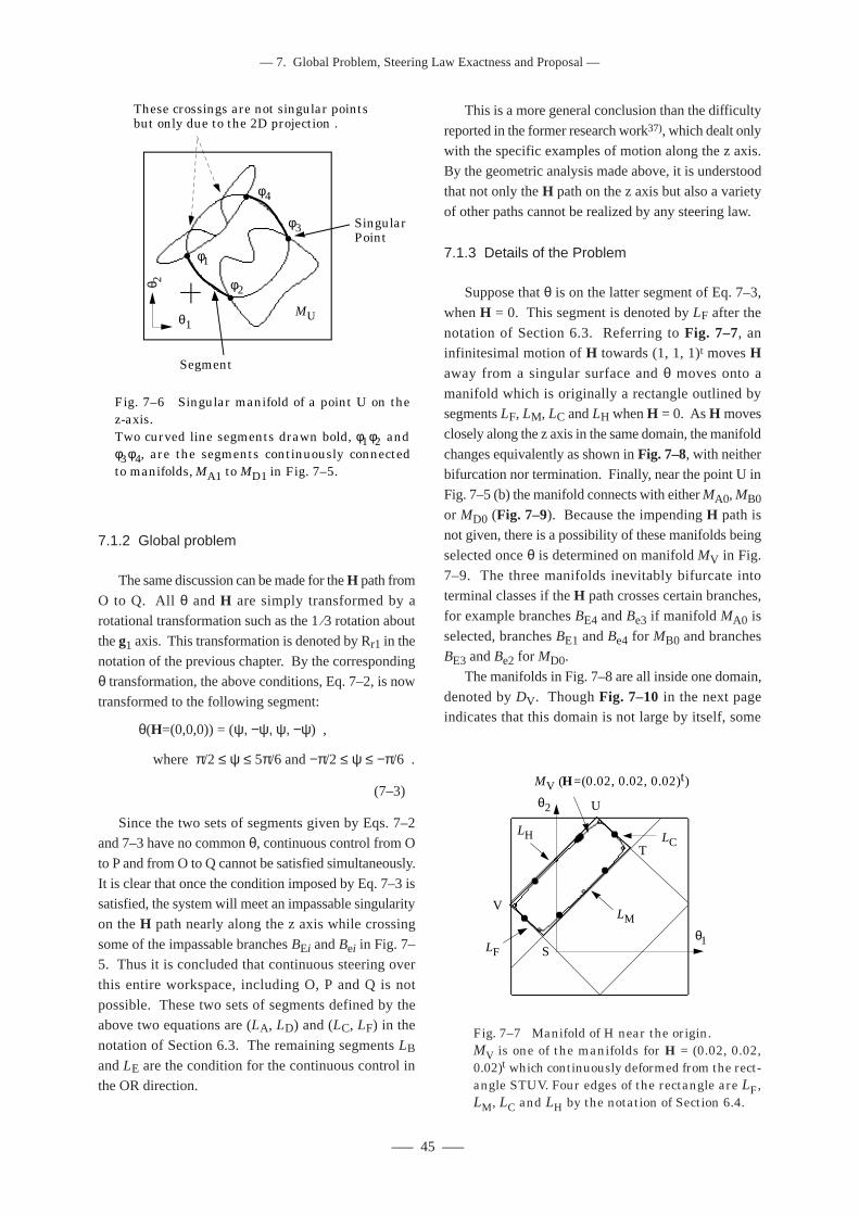
––– 45 –––
–– 7. Global Problem, Steering Law Exactness and Proposal ––
7.1.2 Global problem
The same discussion can be made for the H path from
O to Q. All θ and H are simply transformed by arotational transformation such as the 1 ⁄3 rotation about
the g1 axis. This transformation is denoted by Rr1 in the
notation of the previous chapter. By the correspondingθ transformation, the above conditions, Eq. 7–2, is now
transformed to the following segment:
θ(H=(0,0,0)) = (ψ, −ψ, ψ, −ψ) ,
where π/2 ≤ ψ ≤ 5π/6 and −π/2 ≤ ψ ≤ −π/6 .
(7–3)
Since the two sets of segments given by Eqs. 7–2and 7–3 have no common θ, continuous control from O
to P and from O to Q cannot be satisfied simultaneously.
It is clear that once the condition imposed by Eq. 7–3 issatisfied, the system will meet an impassable singularity
on the H path nearly along the z axis while crossing
some of the impassable branches BEi and Bei in Fig. 7–5. Thus it is concluded that continuous steering over
this entire workspace, including O, P and Q is not
possible. These two sets of segments defined by theabove two equations are (LA, LD) and (LC, LF) in the
notation of Section 6.3. The remaining segments LB
and LE are the condition for the continuous control inthe OR direction.
This is a more general conclusion than the difficulty
reported in the former research work37), which dealt only
with the specific examples of motion along the z axis.By the geometric analysis made above, it is understood
that not only the H path on the z axis but also a variety
of other paths cannot be realized by any steering law.
7.1.3 Details of the Problem
Suppose that θ is on the latter segment of Eq. 7–3,
when H = 0. This segment is denoted by LF after the
notation of Section 6.3. Referring to Fig. 7–7, aninfinitesimal motion of H towards (1, 1, 1)t moves Haway from a singular surface and θ moves onto a
manifold which is originally a rectangle outlined bysegments LF, LM, LC and LH when H = 0. As H moves
closely along the z axis in the same domain, the manifold
changes equivalently as shown in Fig. 7–8, with neitherbifurcation nor termination. Finally, near the point U in
Fig. 7–5 (b) the manifold connects with either MA0, MB0or MD0 (Fig. 7–9). Because the impending H path isnot given, there is a possibility of these manifolds being
selected once θ is determined on manifold MV in Fig.
7–9. The three manifolds inevitably bifurcate intoterminal classes if the H path crosses certain branches,
for example branches BE4 and Be3 if manifold MA0 is
selected, branches BE1 and Be4 for MB0 and branchesBE3 and Be2 for MD0.
The manifolds in Fig. 7–8 are all inside one domain,
denoted by DV. Though Fig. 7–10 in the next pageindicates that this domain is not large by itself, some
Fig. 7–6 Singular manifold of a point U on thez-axis.Two curved line segments drawn bold, φ1φ2 andφ3φ4, are the segments continuously connectedto manifolds, MA1 to MD1 in Fig. 7–5.
θ1
θ 2
These crossings are not singular points but only due to the 2D projection .
Singular Point
Segment
φ1
φ2
φ3
φ4
MU
θ1
MV (H=(0.02, 0.02, 0.02)t)
LF
LCLH
LM
S
T
U
V
θ2
Fig. 7–7 Manifold of H near the origin.MV is one of the manifolds for H = (0.02, 0.02,0.02)t which continuously deformed from the rect-angle STUV. Four edges of the rectangle are LF,LM, LC and LH by the notation of Section 6.4.
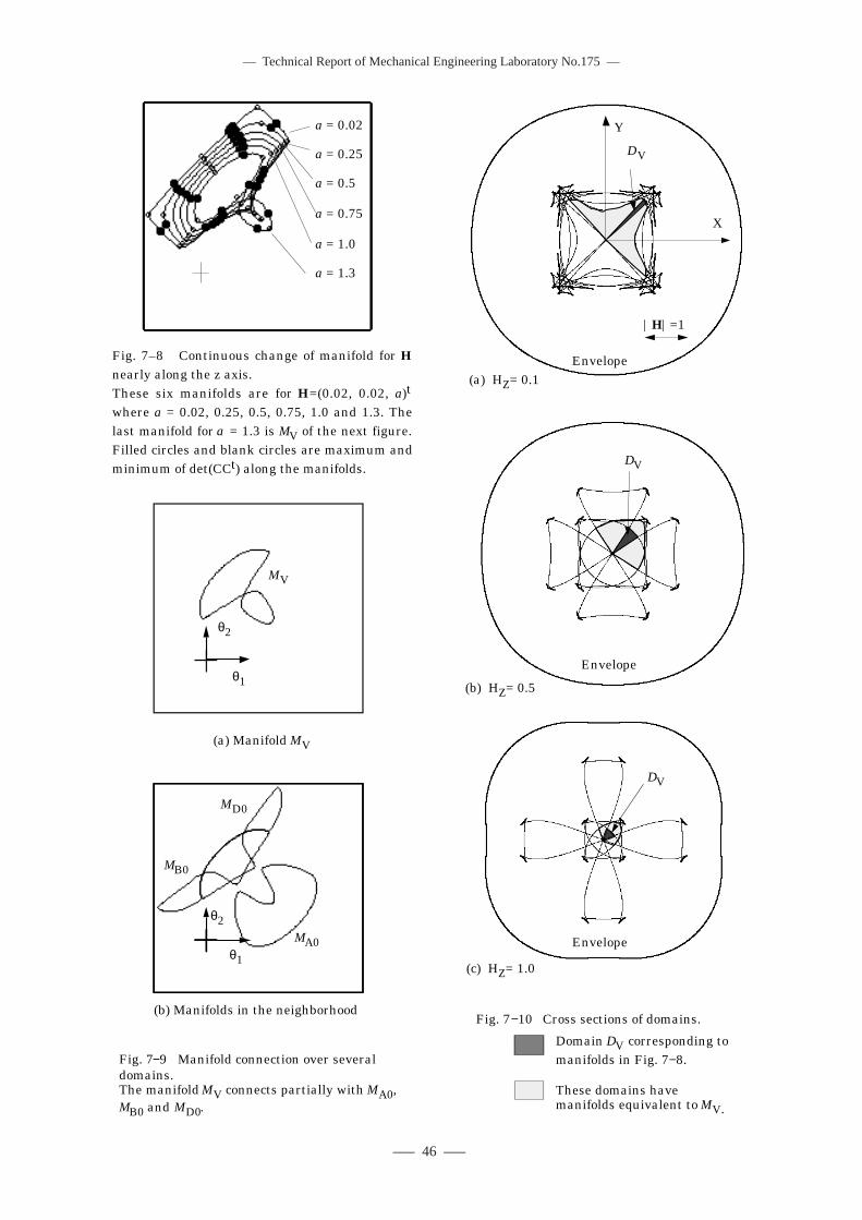
–– Technical Report of Mechanical Engineering Laboratory No.175 ––
––– 46 –––
Fig. 7−9 Manifold connection over several domains.The manifold MV connects partially with MA0, MB0 and MD0.
MV
θ1
θ2
(a) Manifold MV
MB0
MA0
MD0
θ1
θ2
(b) Manifolds in the neighborhood
Fig. 7–8 Continuous change of manifold for H nearly along the z axis.These six manifolds are for H=(0.02, 0.02, a)t where a = 0.02, 0.25, 0.5, 0.75, 1.0 and 1.3. The last manifold for a = 1.3 is MV of the next figure. Filled circles and blank circles are maximum and minimum of det(CCt) along the manifolds.
a = 1.0
a = 0.02
a = 0.25
a = 0.5
a = 0.75
a = 1.3
(a) HZ= 0.1
X
Y
|H|=1
DV
Envelope
DV
(c) HZ= 1.0
Envelope
DV
(b) HZ= 0.5
Envelope
Domain DV corresponding to manifolds in Fig. 7−8.
These domains have manifolds equivalent to MV.
Fig. 7−10 Cross sections of domains.
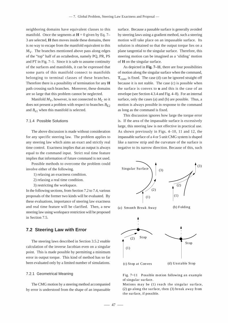
––– 47 –––
–– 7. Global Problem, Steering Law Exactness and Proposal ––
surface. Because a passable surface is generally avoided
by steering laws using a gradient method, such a steering
motion will take place on an impassable surface. Itssolution is obtained so that the output torque lies on a
plane tangential to the singular surface. Therefore, this
steering motion can be imagined as a ‘sliding’ motionof H on the singular surface.
As depicted in Fig. 7–11, there are four possibilities
of motion along the singular surface when the command,Tcom, is fixed. The case (d) can be ignored straight off
because it is not stable. The case (c) is possible when
the surface is convex to u and this is the case of anenvelope (see Section 4.3.4 and Fig. 4–8). For an internal
surface, only the cases (a) and (b) are possible. Thus, a
motion is always possible in response to the commandas long as the command is fixed.
This discussion ignores how large the torque error
is. If the area of the impassable surface is excessivelylarge, this steering law is not effective in practical use.
As shown previously in Figs. 4–10, 11 and 12, the
impassable surface of a 4 or 5 unit CMG system is shapedlike a narrow strip and the curvature of the surface is
negative to its narrow direction. Because of this, such
neighboring domains have equivalent classes to this
manifold. Once the segments at H = 0 given by Eq. 7–
3 are selected, H then moves inside these domains, thereis no way to escape from the manifold equivalent to this
MV. The branches mentioned above pass along edges
of the “top” half of an octahedron, namely PQ, PR, PSand PT in Fig. 7–1. Since it is safe to assume continuity
of the surfaces and manifolds, it can be expressed that
some parts of this manifold connect to manifoldsbelonging to terminal classes of these branches.
Therefore there is a possibility of termination for any Hpath crossing such branches. Moreover, these domainsare so large that this problem cannot be neglected.
Manifold MV, however, is not connected to MC so it
does not present a problem with respect to branches BE2and Be1 when this manifold is selected.
7.1.4 Possible Solutions
The above discussion is made without consideration
for any specific steering law. The problem applies toany steering law which aims an exact and strictly real
time control. Exactness implies that an output is always
equal to the command input. Strict real time featureimplies that information of future command is not used.
Possible methods to overcome the problem could
involve either of the following. 1) relaxing an exactness condition.
2) relaxing a real time condition.
3) restricting the workspace.In the following sections, from Section 7.2 to 7.4, various
proposals of the former two kinds will be evaluated. By
these evaluations, importance of steering law exactnessand real time feature will be clarified. Then, a new
steering law using workspace restriction will be proposed
in Section 7.5.
7.2 Steering Law with Error
The steering laws described in Section 3.5.2 enable
calculation of the inverse Jacobian even on a singular
point. This is made possible by permitting a minimumerror in output torque. This kind of method has so far
been evaluated only by a limited number of simulations.
7.2.1 Geometrical Meaning
The CMG motion by a steering method accompaniedby error is understood from the shape of an impassable
(1)
(2)
(3)
(a) Smooth Break Away
Singular Surface
(b) Folding
(1)
(2)
(3)
Fig. 7−11 Possible motion following an exampleof singular surface. Motions may be (1) reach the singular surface,(2) go along the surface, then (3) break away fromthe surface, if possible.
(c) Stop at Convex
Stop
(1)
(2)
(d) Unstable Stop
Stop
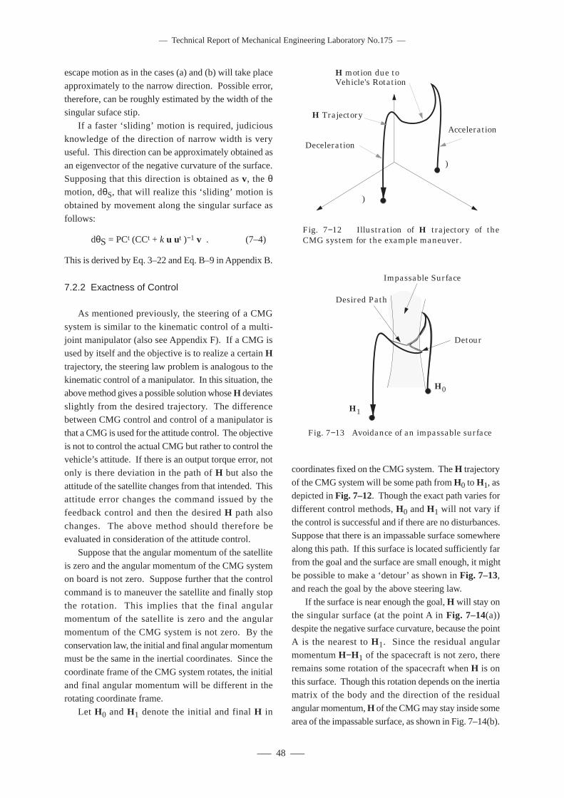
–– Technical Report of Mechanical Engineering Laboratory No.175 ––
––– 48 –––
coordinates fixed on the CMG system. The H trajectory
of the CMG system will be some path from H0 to H1, asdepicted in Fig. 7–12. Though the exact path varies for
different control methods, H0 and H1 will not vary if
the control is successful and if there are no disturbances.Suppose that there is an impassable surface somewhere
along this path. If this surface is located sufficiently far
from the goal and the surface are small enough, it mightbe possible to make a ‘detour’ as shown in Fig. 7–13,and reach the goal by the above steering law.
If the surface is near enough the goal, H will stay onthe singular surface (at the point A in Fig. 7–14(a))
despite the negative surface curvature, because the point
A is the nearest to H1. Since the residual angularmomentum H−H1 of the spacecraft is not zero, there
remains some rotation of the spacecraft when H is on
this surface. Though this rotation depends on the inertiamatrix of the body and the direction of the residual
angular momentum, H of the CMG may stay inside some
area of the impassable surface, as shown in Fig. 7–14(b).
escape motion as in the cases (a) and (b) will take place
approximately to the narrow direction. Possible error,
therefore, can be roughly estimated by the width of thesingular suface stip.
If a faster ‘sliding’ motion is required, judicious
knowledge of the direction of narrow width is veryuseful. This direction can be approximately obtained as
an eigenvector of the negative curvature of the surface.
Supposing that this direction is obtained as v, the θmotion, dθS, that will realize this ‘sliding’ motion is
obtained by movement along the singular surface as
follows:
dθS = PCt (CCt + k u ut )−1 v . (7–4)
This is derived by Eq. 3–22 and Eq. B–9 in Appendix B.
7.2.2 Exactness of Control
As mentioned previously, the steering of a CMG
system is similar to the kinematic control of a multi-joint manipulator (also see Appendix F). If a CMG is
used by itself and the objective is to realize a certain Htrajectory, the steering law problem is analogous to thekinematic control of a manipulator. In this situation, the
above method gives a possible solution whose H deviates
slightly from the desired trajectory. The differencebetween CMG control and control of a manipulator is
that a CMG is used for the attitude control. The objective
is not to control the actual CMG but rather to control thevehicle’s attitude. If there is an output torque error, not
only is there deviation in the path of H but also the
attitude of the satellite changes from that intended. Thisattitude error changes the command issued by the
feedback control and then the desired H path also
changes. The above method should therefore beevaluated in consideration of the attitude control.
Suppose that the angular momentum of the satellite
is zero and the angular momentum of the CMG systemon board is not zero. Suppose further that the control
command is to maneuver the satellite and finally stop
the rotation. This implies that the final angularmomentum of the satellite is zero and the angular
momentum of the CMG system is not zero. By the
conservation law, the initial and final angular momentummust be the same in the inertial coordinates. Since the
coordinate frame of the CMG system rotates, the initial
and final angular momentum will be different in therotating coordinate frame.
Let H0 and H1 denote the initial and final H in
Fig. 7−13 Avoidance of an impassable surface
Impassable Surface
Desired Path
Detour
H0
H1
Fig. 7−12 Illustration of H trajectory of the CMG system for the example maneuver.
H Trajectory
H0
H1
Acceleration
Deceleration
H motion due to Vehicle's Rotation
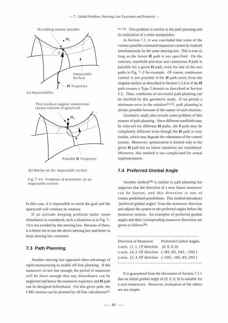
––– 49 –––
–– 7. Global Problem, Steering Law Exactness and Proposal ––
In this case, it is impossible to reach the goal and the
spacecraft will continue its rotation.If an attitude keeping problem under some
disturbance is considered, such a situations as in Fig. 7–
14 is not avoided by this steering law. Because of these,it is better not to use the above steering law and better to
keep steering law exactness.
7.3 Path Planning
Another steering law approach takes advantage ofrapid maneuvering to enable off-line planning. If the
maneuver occurs fast enough, the period of maneuver
will be short enough that any disturbance can beneglected and hence the maneuver trajectory and H path
can be designed beforehand. For this given path, the
CMG motion can be planned by off-line calculations42,
43, 44). This problem is similar to the path planning and
its realization of a robot manipulator.
In Section 7.1, it was concluded that some of thevarious possible command sequences cannot be realized
simultaneously by the same steering law. This is true as
long as the future H path is not specified. On thecontrary, manifold selection and continuous θ path is
possible for a given H path, even for one of the two
paths in Fig. 7–2 for example. Of course, continuouscontrol is not possible if the H path starts from the
singular surface as described in Section 5.5.6 or if the Hpath crosses a Type 2 domain as described in Section5.5. Thus, conditions of successful path planning can
be clarified by this geometric study. If we permit a
minimum error in the solution42,43), path planning isalways possible because of the nature of such motions.
Geometric study also reveals some problem of this
manner of path planning. Since different manifolds maybe selected for different H paths, the θ path may be
completely different even though the H path is very
similar, which may degrade the robustness of the controlsystem. Moreover, optimization is limited only to the
given H path but no future situations are considered.
Moreover, this method is too complicated for actualimplementation.
7.4 Preferred Gimbal Angle
Another method38) is similar to path planning but
supposes that the direction of a near future maneuvercan be known, and this direct ion is one of
certain predefined possibilities. This method introduces
‘preferred gimbal angles’ from the maneuver directionand adjusts the system to the preferred angles before the
maneuver motion. An examples of preferred gimbal
angles and their corresponding maneuver directions aregiven as follows38):
––––––––––––––––––––––––––––––––––––––––––Direction of Maneuver Preferred Gimbal Angles
z-axis, (1, 1, 1)t direction (0, 0, 0, 0)
x-axis, (4, 2, 0)t direction (−π⁄3, π⁄3, 2π⁄3, −2π⁄3 )y-axis, (2, 4, 0)t direction (−2π⁄3, −π⁄3, π⁄3, 2π⁄3 )
––––––––––––––––––––––––––––––––––––––––––––
It is guaranteed from the discussion of Section 7.1.1
that an initial gimbal angle of (0, 0, 0, 0) is suitable for
z-axis maneuvers. However, evaluation of the othersare not simple.
Fig. 7−14 Problems of movement on an impassable surface.
H1
No sliding motion possible
Impassable Surface
H Trajectory
A
(a) Impassability
H1
Possible H Trajectory
This residual angular momentum causes rotation of spacecraft
(b) Motion on the impassable surface
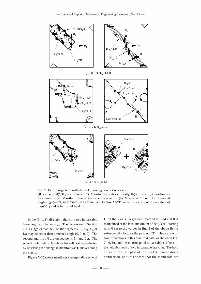
–– Technical Report of Mechanical Engineering Laboratory No.175 ––
––– 50 –––
Hx=0
HX=1.0HX=0
HX=1.0
A(θ0), B
A(θ0)
B
θ1
θ3
θ2
θ4
(a) 0.0 ≤ HX ≤ 1.0
HX=1.0
HX=1.4
HX=1.2
B, CHX=1.0
HX=1.2
HX=1.4
B
C
Connection
(b) 1.0 ≤ HX ≤ 1.4
Fig. 7−15 Change in manifolds for H moving along the x axis.(H = (HX, 0, 0)t, HX step size = 0.2). Manifolds are drawn in (θ1, θ3) and (θ2, θ4) coordinates as shown in (a). Manifold bifurcations are observed in (b). Motion of θ from the preferredangles θ0=(−π ⁄ 3, π ⁄ 3, 2π ⁄ 3, −2π ⁄ 3) follows the line ABCD, which is a trace of the maxima of det(CCt) and is indicated by dots.
HX=1.4
HX=2.6
HX=1.4
HX=2.6C
D
(c) 1.4 ≤ HX ≤ 2.6
In the (1, 1, 1)t direction, there are two impassable
branches, i.e., BE2 and Be1. The discussion in Section7.1.3 suggests that the θ on the segments LF, LM, LC or
LH may be better than preferred angle (0, 0, 0, 0). The
second and third θ are on segments LL and LM. Thesecond preferred θ in the above list will next be evaluated
by observing the change in manifolds as H moves along
the x axis.Figure 7–15 shows manifolds corresponding several
H on the x axis. A gradient method is used and θ is
maintained at the local maximum of det(CCt). Startingwith θ set to the values in line 2 of the above list, θsubsequently follows the path ABCD. There are only
two bifurcations in this manifold path, as shown in Fig.7–15(b), and these correspond to passable surfaces in
the neighborhood of two impassable branches. The bold
curve in the left plot of Fig. 7–15(b) indicates aconnection, and this shows that the manifolds are
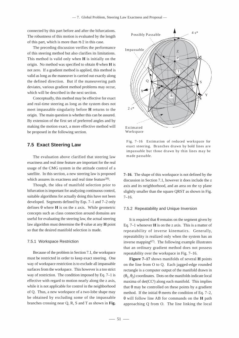
––– 51 –––
–– 7. Global Problem, Steering Law Exactness and Proposal ––
connected by this part before and after the bifurcations.
The robustness of this motion is evaluated by the length
of this part, which is more than π ⁄2 in this case.The preceding discussion verifies the performance
of this steering method but also clarifies its limitations.
This method is valid only when H is initially on theorigin. No method was specified to obtain θ when H is
not zero. If a gradient method is applied, this method is
valid as long as the maneuver is carried out exactly alongthe defined direction. But if the maneuvering path
deviates, various gradient method problems may occur,
which will be described in the next section.Conceptually, this method may be effective for exact
and real-time steering as long as the system does not
meet impassable singularity before H returns to theorigin. The main question is whether this can be assured.
By extension of the first set of preferred angles and by
making the motion exact, a more effective method willbe proposed in the following section.
7.5 Exact Steering Law
The evaluation above clarified that steering law
exactness and real time feature are important for the realusage of the CMG system in the attitude control of a
satellite. In this section, a new steering law is proposed
which assures its exactness and real time feature39).Though, the idea of manifold selection prior to
bifurcation is important for analyzing continuous control,
suitable algorithms for actually doing this have not beendeveloped. Segments defined by Eqs. 7–1 and 7–2 only
defines θ where H is on the z axis. While geometric
concepts such as class connection around domains areuseful for evaluating the steering law, the actual steering
law algorithm must determine the θ value at any H point
so that the desired manifold selection is made.
7.5.1 Workspace Restriction
Because of the problem in Section 7.1, the workspace
must be restricted in order to keep exact steering. One
way of workspace restriction is to exclude all impassablesurfaces from the workspace. This however is a too strict
way of restriction. The condition imposed by Eq. 7–1 is
effective with regard to motion nearly along the z axis,while it is not applicable for control in the neighborhood
of Q. Thus, a new workspace of a two-lobe shape may
be obtained by excluding some of the impassablebranches crossing near Q, R, S and T as shown in Fig.
7–16. The shape of this workspace is not defined by the
discussion in Section 7.1, however it does include the zaxis and its neighborhood, and an area on the xy plane
slightly smaller than the square QRST as shown in Fig.
7–16.
7.5.2 Repeatability and Unique Inversion
It is required that θ remains on the segment given by
Eq. 7–1 whenever H is on the z axis. This is a matter of
repeatability of inverse kinematics. Generally,repeatability is realized only when the system has an
inverse mapping67). The following example illustrates
that an ordinary gradient method does not possessrepeatability over the workspace in Fig. 7–16.
Figure 7–17 shows manifolds of several H points
on the line from O to Q. Each jagged-edge roundedrectangle is a computer output of the manifold drawn in
(θ1, θ2) coordinates. Dots on the manifolds indicate local
maxima of det(CCt) along each manifold. This impliesthat θ may be controlled on these points by a gradient
method. If the initial θ meets the condition of Eq. 7–2,
θ will follow line AB for commands on the H pathapproaching Q from O. The line linking the local
XY
Z
Possibly Passable
Impassable
Estimated Workspace
P
S
T
Q
R
4 s*
2 c*
Fig. 7–16 Estimation of reduced workspace for exact steering. Branches drawn by bold lines are impassable but those drawn by thin lines may be made passable.
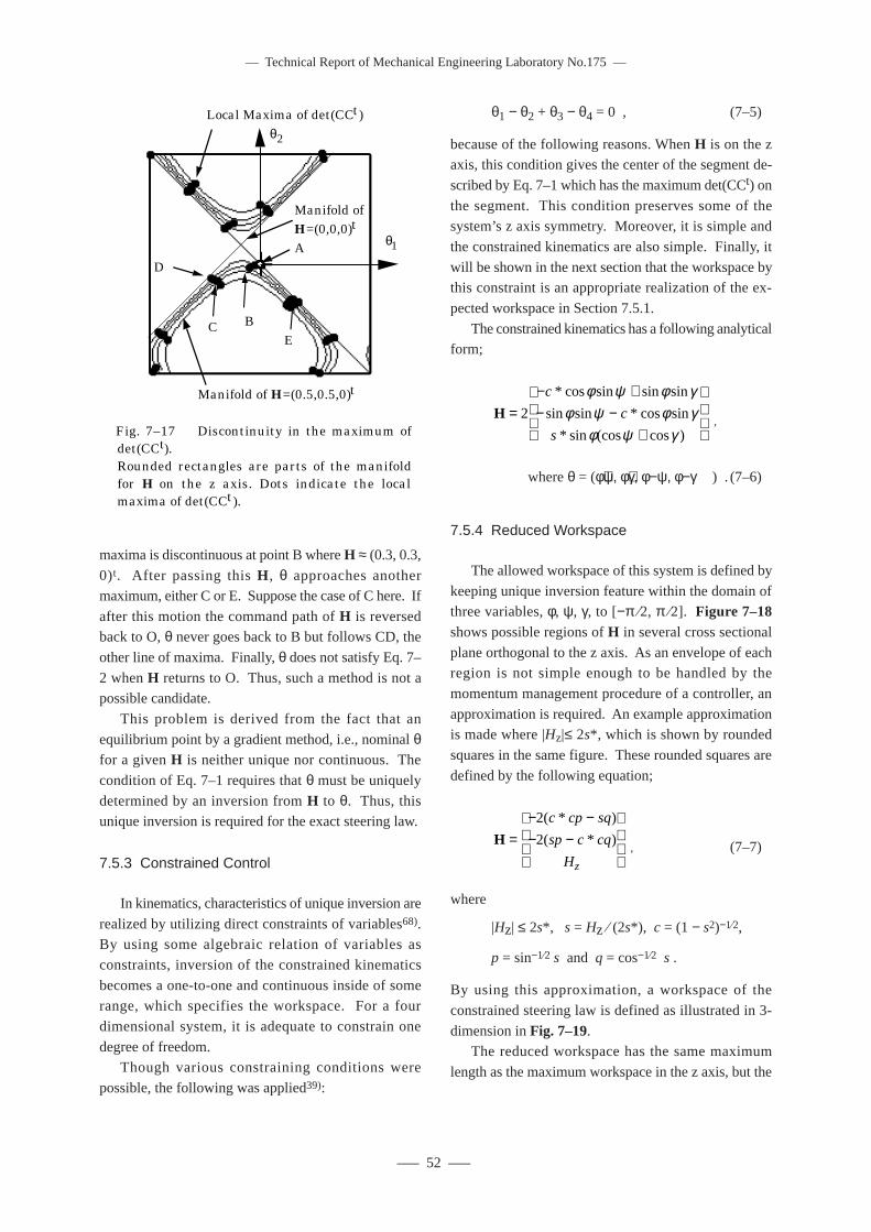
–– Technical Report of Mechanical Engineering Laboratory No.175 ––
––– 52 –––
maxima is discontinuous at point B where H ≈ (0.3, 0.3,
0)t. After passing this H , θ approaches anothermaximum, either C or E. Suppose the case of C here. If
after this motion the command path of H is reversedback to O, θ never goes back to B but follows CD, the
other line of maxima. Finally, θ does not satisfy Eq. 7–
2 when H returns to O. Thus, such a method is not apossible candidate.
This problem is derived from the fact that an
equilibrium point by a gradient method, i.e., nominal θfor a given H is neither unique nor continuous. The
condition of Eq. 7–1 requires that θ must be uniquely
determined by an inversion from H to θ. Thus, thisunique inversion is required for the exact steering law.
7.5.3 Constrained Control
In kinematics, characteristics of unique inversion are
realized by utilizing direct constraints of variables68).By using some algebraic relation of variables as
constraints, inversion of the constrained kinematics
becomes a one-to-one and continuous inside of somerange, which specifies the workspace. For a four
dimensional system, it is adequate to constrain one
degree of freedom.Though various constraining conditions were
possible, the following was applied39):
θ1 − θ2 + θ3 − θ4 = 0 , (7–5)
because of the following reasons. When H is on the zaxis, this condition gives the center of the segment de-
scribed by Eq. 7–1 which has the maximum det(CCt) on
the segment. This condition preserves some of thesystem’s z axis symmetry. Moreover, it is simple and
the constrained kinematics are also simple. Finally, it
will be shown in the next section that the workspace bythis constraint is an appropriate realization of the ex-
pected workspace in Section 7.5.1.
The constrained kinematics has a following analyticalform;
H =− +− −
+
2
c
c
s
* cos sin sin sin
sin sin * cos sin
* sin (cos cos )
φ ψ φ γφ ψ φ γ
φ ψ γ ,
where θ = (φ+ψ, φ+γ, φ−ψ, φ−γ) . (7–6)
7.5.4 Reduced Workspace
The allowed workspace of this system is defined by
keeping unique inversion feature within the domain ofthree variables, φ, ψ, γ, to [−π ⁄2, π ⁄2]. Figure 7–18shows possible regions of H in several cross sectional
plane orthogonal to the z axis. As an envelope of eachregion is not simple enough to be handled by the
momentum management procedure of a controller, an
approximation is required. An example approximationis made where |Hz|≤ 2s*, which is shown by rounded
squares in the same figure. These rounded squares are
defined by the following equation;
H =− −− −
2
2
( * )
( * )
c cp sq
sp c cq
Hz
, (7–7)
where
|Hz| ≤ 2s*, s = Hz ⁄ (2s*), c = (1 − s2)−1⁄2,
p = sin−1⁄2 s and q = cos−1⁄2 s .
By using this approximation, a workspace of the
constrained steering law is defined as illustrated in 3-
dimension in Fig. 7–19.The reduced workspace has the same maximum
length as the maximum workspace in the z axis, but the
Fig. 7–17 Discontinuity in the maximum of det(CCt).Rounded rectangles are parts of the manifold for H on the z axis. Dots indicate the local maxima of det(CCt).
θ1
θ2
Local Maxima of det(CCt)
A
BC
D
E
Manifold of H=(0,0,0)t
Manifold of H=(0.5,0.5,0)t
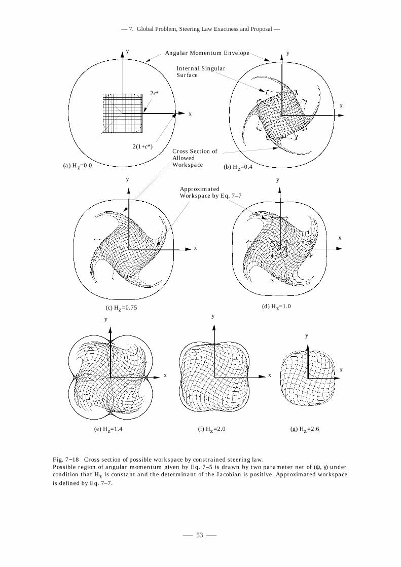
––– 53 –––
–– 7. Global Problem, Steering Law Exactness and Proposal ––
Fig. 7−18 Cross section of possible workspace by constrained steering law.Possible region of angular momentum given by Eq. 7–5 is drawn by two parameter net of (ψ, γ) undercondition that Hz is constant and the determinant of the Jacobian is positive. Approximated workspaceis defined by Eq. 7–7.
(a) Hz=0.0 (b) Hz=0.4
(c) Hz=0.75 (d) Hz=1.0
(e) Hz=1.4 (f) Hz=2.0 (g) Hz=2.6
Cross Section of Allowed Workspace
Approximated Workspace by Eq. 7–7
Angular Momentum Envelope
Internal Singular Surface
2c*
2(1+c*)
x
y
x
y
x
y
x
y
x
y
x
y
y
x
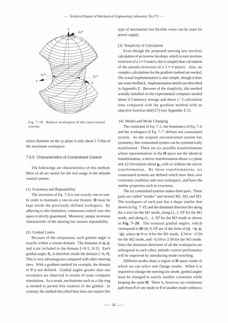
–– Technical Report of Mechanical Engineering Laboratory No.175 ––
––– 54 –––
minor diameter on the xy plane is only about 1 ⁄3 that ofthe maximum workspace.
7.5.5 Characteristics of Constrained Control
The followings are characteristics of this method.
Most of all are useful for the real usage in the attitudecontrol system.
(1) Exactness and RepeatabilityThe inversion of Eq. 7–6 is not exactly one-to-one.
In order to maintain a one-to-one feature, H must be
kept inside the previously defined workspace. Byadhering to this limitation, continuous control over this
space is strictly guaranteed. Moreover, unique inversion
characteristic of the steering law assures repeatability.
(2) Gimbal Limits
Because of the uniqueness, each gimbal angle isexactly within a certain domain. The domains of φ, ψ,
and γ are included in the domain [−π ⁄2, π ⁄2]. Each
gimbal angle, θi, is therefore inside the domain [−π, π].This is very advantageous compared with other steering
laws. With a gradient method for example, the domain
of θ is not defined. Gimbal angles greater than onerevolution are observed in results of some computer
simulations. As a result, mechanisms such as a slip ring
is needed to permit free rotation of the gimbal. Incontrast, the method described here does not require this
type of mechanism but flexible wires can be used for
power supply.
(3) Simplicity of Calculation
Even though the proposed steering law involves
calculation of an inverse Jacobian, which in turn involvesinversion of a 3 × 3 matrix, this is simpler than calculation
of the pseudo-inversion of a 3 × 4 matrix. Also, no
complex calculations for the gradient method are needed.The actual implementation is also simple, though it does
use some feedback. Implementation details are described
in Appendix E. Because of the simplicity, this methodactually installed on the experimental computer needed
about 2⁄ 3 memory storage and about 1 ⁄ 2 calculation
time compared with the gradient method with an
objective function det(CCt) (see Appendix E.5).
(4) Modes and Mode Changing
The constraint of Eq. 7–5, the kinematics of Eq. 7–6and the workspace of Eq. 7–7 defines one constrained
system. As the original unconstrained system has
symmetry, this constrained system can be symmetricallytransformed. There are six possible transformations
whose representations in the H space are the identical
transformation, a mirror transformation about x-z planeand ±2/3π rotation about g1 with or without the mirror
transformation. By those transformations, six
constrained systems are defined which have their ownconstraint condition and own workspace, and have the
similar properties such as exactness.
The six constrained systems makes three pairs. Thesepairs are called “modes” and termed M1, M2 and M3.
The workspace of each pair has a shape similar that
shown in Fig. 7–19, and the dominant direction lies alongthe z-axis for the M1 mode, along (1, 1, 0)t for the M2
mode, and along (1, –1, 0)t for the M3 mode as shown
in Fig. 7–20. The nominal gimbal angles, whichcorrespond to H=(0, 0, 0)t are of the form of (ψ, −ψ, ψ,−ψ), where ψ=0 or π for the M1 mode, 1/3π or −2/3πfor the M2 mode, and −1/3π or 2/3π for the M3 mode.Since the dominant directions of all the workspaces are
orthogonal to each other, attitude control performance
will be improved by introducing mode switching.Different modes share a region in H space inside of
which we can select and change modes. When it is
required to change the steering law mode, gimbal anglesmust be changed to satisfy another constraint while
keeping the same H. There is, however, no continuous
path from θ of one mode to θ of another mode without a
Fig. 7−19 Reduce workspace of the constrained system.
z4s*
x y
2c*2c*
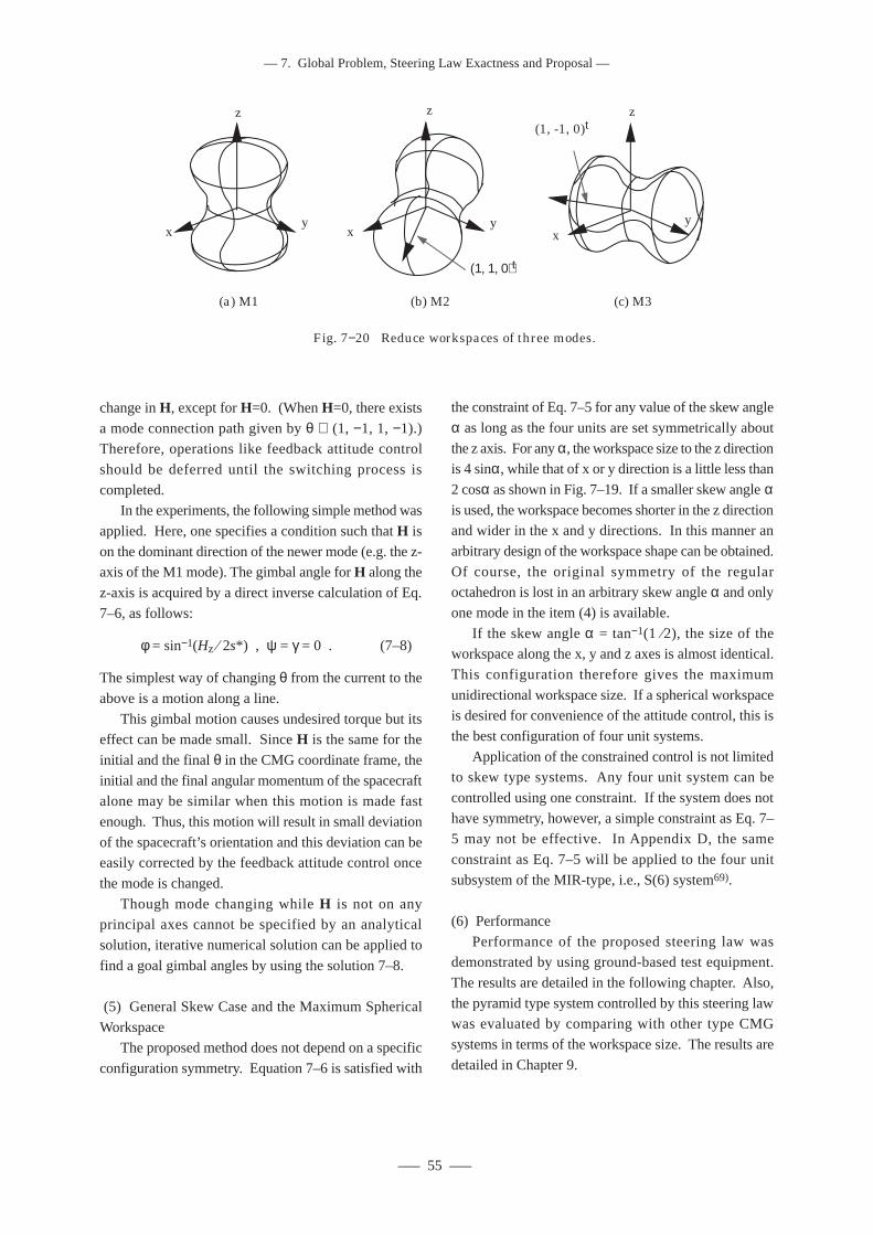
––– 55 –––
–– 7. Global Problem, Steering Law Exactness and Proposal ––
(b) M2
(1, 1, 0)t
z
xy
(c) M3
(1, -1, 0)tz
xy
(a) M1
z
xy
Fig. 7−20 Reduce workspaces of three modes.
change in H, except for H=0. (When H=0, there exists
a mode connection path given by θ ∝ (1, −1, 1, −1).)Therefore, operations like feedback attitude control
should be deferred until the switching process is
completed.In the experiments, the following simple method was
applied. Here, one specifies a condition such that H is
on the dominant direction of the newer mode (e.g. the z-axis of the M1 mode). The gimbal angle for H along the
z-axis is acquired by a direct inverse calculation of Eq.
7–6, as follows:
φ = sin−1(Hz ⁄ 2s*) , ψ = γ = 0 . (7–8)
The simplest way of changing θ from the current to the
above is a motion along a line.
This gimbal motion causes undesired torque but itseffect can be made small. Since H is the same for the
initial and the final θ in the CMG coordinate frame, the
initial and the final angular momentum of the spacecraftalone may be similar when this motion is made fast
enough. Thus, this motion will result in small deviation
of the spacecraft’s orientation and this deviation can beeasily corrected by the feedback attitude control once
the mode is changed.
Though mode changing while H is not on anyprincipal axes cannot be specified by an analytical
solution, iterative numerical solution can be applied to
find a goal gimbal angles by using the solution 7–8.
(5) General Skew Case and the Maximum Spherical
WorkspaceThe proposed method does not depend on a specific
configuration symmetry. Equation 7–6 is satisfied with
the constraint of Eq. 7–5 for any value of the skew angle
α as long as the four units are set symmetrically about
the z axis. For any α, the workspace size to the z directionis 4 sinα, while that of x or y direction is a little less than
2 cosα as shown in Fig. 7–19. If a smaller skew angle αis used, the workspace becomes shorter in the z directionand wider in the x and y directions. In this manner an
arbitrary design of the workspace shape can be obtained.
Of course, the original symmetry of the regularoctahedron is lost in an arbitrary skew angle α and only
one mode in the item (4) is available.
If the skew angle α = tan−1(1 ⁄2), the size of theworkspace along the x, y and z axes is almost identical.
This configuration therefore gives the maximum
unidirectional workspace size. If a spherical workspaceis desired for convenience of the attitude control, this is
the best configuration of four unit systems.
Application of the constrained control is not limitedto skew type systems. Any four unit system can be
controlled using one constraint. If the system does not
have symmetry, however, a simple constraint as Eq. 7–5 may not be effective. In Appendix D, the same
constraint as Eq. 7–5 will be applied to the four unit
subsystem of the MIR-type, i.e., S(6) system69).
(6) Performance
Performance of the proposed steering law wasdemonstrated by using ground-based test equipment.
The results are detailed in the following chapter. Also,
the pyramid type system controlled by this steering lawwas evaluated by comparing with other type CMG
systems in terms of the workspace size. The results are
detailed in Chapter 9.

–– Technical Report of Mechanical Engineering Laboratory No.175 ––
––– 56 –––
––– 57 –––
–– 8. Ground Experiments ––
Chapter 8
Ground Experiments
The previous chapters dealt only with CMG systemswhile aiming primarily at a geometric understanding of
the CMG motion and leaving quantitative matters
neglected. In this chapter, a CMG-based total attitudecontrol system is briefly formulated and in order to
quantitatively verify the steering law performance,
ground experiments were carried out. Test resultsshowed clearly the problems found with typical steering
laws and the performance of the steering law proposed
in the previous chapter.
8.1 Attitude Control
8.1.1 Dynamics
The attitude, namely the orientation of a body can
be represented by various ways70) such as the direction
cosines, the Euler angles, Roll-Pitch-Yaw angles,Rodrigues parameters and Euler parameters. In this
work, representation is made using Euler parameters.
Any attitude is defined as is caused by a singlerotation. The Euler parameters β = (β0, β1, β2, β3)
represent an attitude caused by a single rotation of angle
φ about the axis e = (e1, e2, e3)t:
β0 = cos(φ / 2), (8–1)
βi = ei sin(φ / 2) ,
where i = 1, 2, 3 and |e|=1. As the rotation has three
degree of freedom, there is a constraining condition that
Σ βi2 = 1.Any attitude, which is the result of a rotation a =
(a0, a1, a2, a3) after a rotation b = (b0, b1, b2, b3), is
expressed as a multiplication by a⋅b in the sense of aHamiltonian quarternion as follows:
a⋅b = (a0b0 – a1b1 − a2b2 – a3b3,
a0b1 + a1b0 + a2b3 − a3b2,
a0b2 − a1b3 + a2b0 + a3b1,
a0b3 + a1b2 – a2b1 + a3b0) . (8–2)
The time derivative of β, i.e., dβ ⁄dt is expressed byangular velocity denoted by ωV:
dβ* ⁄ dt = 1 ⁄ 2 (β0 + β* × ωV) , (8–3)
where
β* = (β1, β2, β3)t . (8–4)
This β* is called a vector part of β and regarded as ausual vector in three-dimensional physical space.
The attitude dynamics of a rigid body is represented
in the body’s coordinates by the following Eulerequation:
IV dω ⁄ dt = τ − ωV × p , (8–5)
where IV denotes satellite’s moment of inertia and τdenotes the torque applied to the satellite. This torquecomes from both the outside as a disturbance torque and
from the inside by the CMG system. The vector p is the
total angular momentum of both the satellite and theCMG system and is given by:
p = IV ωV + HCMG . (8–6)
This total angular momentum is conserved in the
inertial coordinates if there is no disturbance torque. Bysubstituting Eq. 8–6 into Eq. 8–5, the ωV×HCMG term
appears. This term is omitted in Eq. 3–5, i.e., the output
equation of the CMG but is evaluated here. Both thekinematic equation and the dynamic equation, Eqs. 8–3
and 8–5, are the describing functions of the system.
8.1.2 Exact Linearization
The system has six independent variables, threecomponents of β* and three components of ωV. The
dynamics is nonlinear as seen by the term ωV×(IVωV)
when Eq. 8–6 is substituted into Eq. 8–5. Nevertheless,it is well known that this nonlinear system can be exactly
linearized with a suitable feedback71, 72).
Let (β*, dβ* ⁄ dt) be state variables and let v be anew input variable. If a real input τ is given as:
––– 57 –––
–– 8. Ground Experiments ––
Chapter 8
Ground Experiments
The previous chapters dealt only with CMG systemswhile aiming primarily at a geometric understanding ofthe CMG motion and leaving quantitative mattersneglected. In this chapter, a CMG-based total attitudecontrol system is briefly formulated and in order toquantitatively verify the steering law performance,ground experiments were carried out. Test resultsshowed clearly the problems found with typical steeringlaws and the performance of the steering law proposedin the previous chapter.
8.1 Attitude Control
8.1.1 Dynamics
The attitude, namely the orientation of a body canbe represented by various ways70) such as the directioncosines, the Euler angles, Roll-Pitch-Yaw angles,Rodrigues parameters and Euler parameters. In thiswork, representation is made using Euler parameters.
Any attitude is defined as is caused by a singlerotation. The Euler parameters β=(β0, β1, β2, β3)represent an attitude caused by a single rotation of angleφ about the axis e = (e1, e2, e3)t:
β0 = cos(φ )1–8(,)2 /
βi = ei sin(φ / 2) ,
where i = 1, 2, 3 and |e|=1. As the rotation has threedegree of freedom, there is a constraining condition thatΣβi
2 = 1.Any attitude, which is the result of a rotation a =
(a0, a1, a2, a3) after a rotation b = (b0, b1, b2, b3), isexpressed as a multiplication by a⋅b in the sense of aHamiltonian quarternion as follows:
a⋅b = (a0b0 – a1b1 − a2b2 – a3b3,
a0b1 + a1b0 + a2b3 − a3b2,
a0b2 − a1b3 + a2b0 + a3b1,
a0b3 + a1b2 – a2b1 + a3b0) . (8–2)
The time derivative of β, i.e., dβ ⁄dt is expressed byangular velocity denoted by ωV:
dβ* ⁄ dt = 1 ⁄ 2 β0 + β*×ωV , (8–3)
where
β* = (β1,β2,β3)t . (8–4)
Thisβ* is called a vector part of β and regarded as ausual vector in three-dimensional physical space.
The attitude dynamics of a rigid body is representedin the body’s coordinates by the following Eulerequation:
IV dω⁄ dt = τ − ωV × p , (8–5)
where IV denotes satellite’s moment of inertia and τdenotes the torque applied to the satellite. This torquecomes from both the outside as a disturbance torque andfrom the inside by the CMG system. The vector p is thetotal angular momentum of both the satellite and theCMG system and is given by:
p = IVωV + HCMG . (8–6)
This total angular momentum is conserved in theinertial coordinates if there is no disturbance torque. Bysubstituting Eq. 8–6 into Eq. 8–5, the ωV×HCMG termappears. This term is omitted in Eq. 3–5, i.e., the outputequation of the CMG but is evaluated here. Both thekinematic equation and the dynamic equation, Eqs. 8–3and 8–5, are the describing functions of the system.
8.1.2 Exact Linearization
The system has six independent variables, threecomponents of β* and three components of ωV. Thedynamics is nonlinear as seen by the term ωV×(IVωV)when Eq. 8–6 is substituted into Eq. 8–5. Nevertheless,it is well known that this nonlinear system can be exactlylinearized with a suitable feedback71, 72).
Let (β*, dβ*⁄ d t ) be state variables and let v be anew input variable. If a real input τ is given as:
ωV
corrected July, 2011
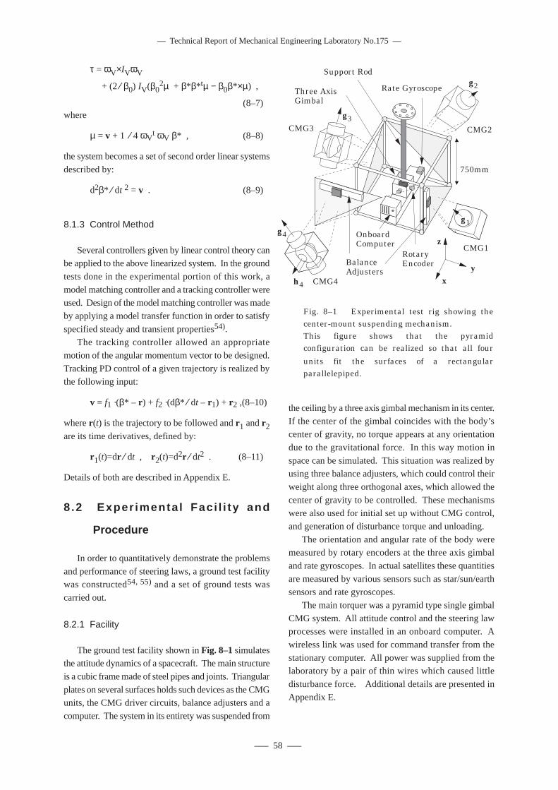
–– Technical Report of Mechanical Engineering Laboratory No.175 ––
––– 58 –––
τ = ωV×IVωV
+ (2 ⁄ β0) IV(β02µ + β*β* tµ − β0β*×µ) ,
(8–7)where
µ = v + 1 ⁄ 4 ωVt ωV β* , (8–8)
the system becomes a set of second order linear systems
described by:
d2β* ⁄ dt 2 = v . (8–9)
8.1.3 Control Method
Several controllers given by linear control theory canbe applied to the above linearized system. In the ground
tests done in the experimental portion of this work, a
model matching controller and a tracking controller wereused. Design of the model matching controller was made
by applying a model transfer function in order to satisfy
specified steady and transient properties54).The tracking controller allowed an appropriate
motion of the angular momentum vector to be designed.
Tracking PD control of a given trajectory is realized bythe following input:
v = f1 ·(β* – r ) + f2 ·(dβ* ⁄ dt – r1) + r2 ,(8–10)
where r (t) is the trajectory to be followed and r1 and r2are its time derivatives, defined by:
r1(t)=dr ⁄ dt , r2(t)=d2r ⁄ dt2 . (8–11)
Details of both are described in Appendix E.
8.2 Exper imenta l Fac i l i t y and
Procedure
In order to quantitatively demonstrate the problems
and performance of steering laws, a ground test facilitywas constructed54, 55) and a set of ground tests was
carried out.
8.2.1 Facility
The ground test facility shown in Fig. 8–1 simulatesthe attitude dynamics of a spacecraft. The main structure
is a cubic frame made of steel pipes and joints. Triangular
plates on several surfaces holds such devices as the CMGunits, the CMG driver circuits, balance adjusters and a
computer. The system in its entirety was suspended from
the ceiling by a three axis gimbal mechanism in its center.
If the center of the gimbal coincides with the body’scenter of gravity, no torque appears at any orientation
due to the gravitational force. In this way motion in
space can be simulated. This situation was realized byusing three balance adjusters, which could control their
weight along three orthogonal axes, which allowed the
center of gravity to be controlled. These mechanismswere also used for initial set up without CMG control,
and generation of disturbance torque and unloading.
The orientation and angular rate of the body weremeasured by rotary encoders at the three axis gimbal
and rate gyroscopes. In actual satellites these quantities
are measured by various sensors such as star/sun/earthsensors and rate gyroscopes.
The main torquer was a pyramid type single gimbal
CMG system. All attitude control and the steering lawprocesses were installed in an onboard computer. A
wireless link was used for command transfer from the
stationary computer. All power was supplied from thelaboratory by a pair of thin wires which caused little
disturbance force. Additional details are presented in
Appendix E.
Fig. 8–1 Experimental test rig showing the center-mount suspending mechanism.This figure shows that the pyramid configuration can be realized so that all four
units fit the surfaces of a rectangular parallelepiped.
Three Axis Gimbal
CMG4
Rotary EncoderBalance
Adjusters
750mm
Onboard Computer
Rate Gyroscope
AAAAAAAAAAAAAAAA
CMG3 CMG2
CMG1
h4
g4
g3
g2
g1
xy
z
Support Rod
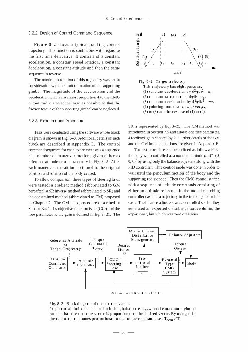
––– 59 –––
–– 8. Ground Experiments ––
8.2.2 Design of Control Command Sequence
Figure 8–2 shows a typical tracking control
trajectory. This function is continuous with regard to
the first time derivative. It consists of a constantacceleration, a constant speed rotation, a constant
deceleration, a constant attitude and then the same
sequence in reverse.The maximum rotation of this trajectory was set in
consideration with the limit of rotation of the supporting
gimbal. The magnitude of the acceleration and thedeceleration which are almost proportional to the CMG
output torque was set as large as possible so that the
friction torque of the supporting gimbal can be neglected.
8.2.3 Experimental Procedure
Tests were conducted using the software whose block
diagram is shown in Fig. 8–3. Additional details of each
block are described in Appendix E. The controlcommand sequence for each experiment was a sequence
of a number of maneuver motions given either as
reference attitude or as a trajectory in Fig. 8–2. Aftereach maneuver, the attitude returned to the original
position and rotation of the body ceased.
To allow comparison, three types of steering lawswere tested: a gradient method (abbreviated to GM
hereafter), a SR inverse method (abbreviated to SR) and
the constrained method (abbreviated to CM) proposedin Chapter 7. The GM uses procedure described in
Section 3.4.1. Its objective function is det(CCt) and the
free parameter is the gain k defined in Eq. 3–21. The
SR is represented by Eq. 3–23. The CM method was
introduced in Section 7.5 and allows one free parameter,
a feedback gain denoted by k. Further details of the GMand the CM implementations are given in Appendix E.
The test procedure can be outlined as follows: First,
the body was controlled at a nominal attitude of β*=(0,0, 0)t by using only the balance adjusters along with the
PID controller. This control mode was done in order to
wait until the pendulum motion of the body and thesupporting rod stopped. Then the CMG control started
with a sequence of attitude commands consisting of
either an attitude reference in the model matchingcontroller case, or a trajectory in the tracking controller
case. The balance adjusters were controlled so that they
generated an expected disturbance torque during theexperiment, but which was zero otherwise.
Fig. 8–2 Target trajectory. This trajectory has eight parts as, (1) constant acceleration by d2φ⁄dt2 = a, (2) constant rate rotation, dφ⁄dt=at1, (3) constant deceleration by d2φ⁄dt2 = −a, (4) pointing control at φ =at1
2+at1t2, (5) to (8) are the reverse of (1) to (4).
Rot
atio
nal
an
gle
φ
time
t1 t2 t1 t3 t1 t1t2 t3
(1)
(2)
(3) (4) (5)
(6)
(7) (8)
Fig. 8–3 Block diagram of the control system.Proportional limiter is used to limit the gimbal rate, ωcom, to the maximum gimbal rate so that the real rate vector is proportional to the desired vector. By using this, the real output becomes proportional to the torque command, i.e., Tcom ⁄⁄ T.
Attitude Command Generator
Attitude Controller
CMG Steering
LawBody
Reference Attitude or
Target Trajectory
Torque Command
TCOMDesired Motion
ω
Torque Output
T
Attitude and Rotational Rate
Pyramid Type CMG
System
Pro-portional Limiter
Balance AdjustersMomentum and
Disturbance Management
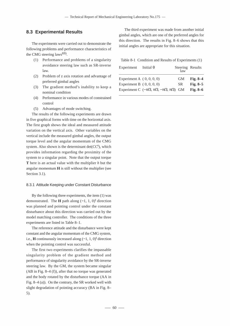
–– Technical Report of Mechanical Engineering Laboratory No.175 ––
––– 60 –––
8.3 Experimental Results
The experiments were carried out to demonstrate the
following problems and performance characteristics of
the CMG steering laws69).(1) Performance and problems of a singularity
avoidance steering law such as SR-inverse
law.(2) Problem of z axis rotation and advantage of
preferred gimbal angles
(3) The gradient method’s inability to keep anominal condition
(4) Performance in various modes of constrained
control(5) Advantages of mode switching.
The results of the following experiments are drawn
in five graphical forms with time on the horizontal axis.The first graph shows the ideal and measured attitude
variation on the vertical axis. Other variables on the
vertical include the measured gimbal angles, the outputtorque level and the angular momentum of the CMG
system. Also shown is the determinant det(CCt), which
provides information regarding the proximity of thesystem to a singular point. Note that the output torque
T here is an actual value with the multiplier h but the
angular momentum H is still without the multiplier (seeSection 3.1).
8.3.1 Attitude Keeping under Constant Disturbance
By the following three experiments, the item (1) was
demonstrated. The H path along (−1, 1, 0)t directionwas planned and pointing control under the constant
disturbance about this direction was carried out by the
model matching controller. The conditions of the threeexperiments are listed in Table 8–1.
The reference attitude and the disturbance were kept
constant and the angular momentum of the CMG system,i.e., H continuously increased along (−1, 1, 0)t direction
when the pointing control was successful.
The first two experiments clarifies the impassablesingularity problem of the gradient method and
performance of singularity avoidance by the SR-inverse
steering law. By the GM, the system became singular(AB in Fig. 8–4 (f)), after that no torque was generated
and the body rotated by the disturbance torque (AA in
Fig. 8–4 (a)). On the contrary, the SR worked well withslight degradation of pointing accuracy (BA in Fig. 8–
5).
The third experiment was made from another initial
gimbal angles, which are one of the preferred angles for
this direction. The results in Fig. 8–6 shows that thisinitial angles are appropriate for this situation.
Table 8-1 Condition and Results of Experiments (1)
Experiment Initial θ Steering Results law
——————————————————————Experiment A ( 0, 0, 0, 0) GM Fig. 8–4Experiment B ( 0, 0, 0, 0) SR Fig. 8–5Experiment C (−π/3, π/3, −π/3, π/3) GM Fig. 8–6——————————————————————
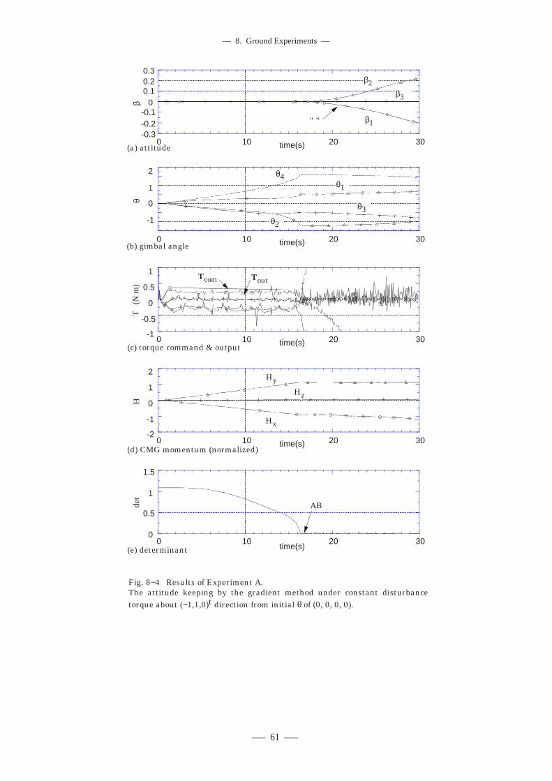
––– 61 –––
–– 8. Ground Experiments ––
Fig. 8−4 Results of Experiment A. The attitude keeping by the gradient method under constant disturbancetorque about (−1,1,0)t direction from initial θ of (0, 0, 0, 0).
AAAAAAAAAAAAAAAAAAAAAAAAAAAAAAAAAAAAAAAAAAAAAAAAAAAA
AAAA
AAAA
AAAA
AAAA
0
0.5
1
1.5
0 10 20 30
det
time(s)(e) determinant
AB
AAAAAAAAAAAAAAAAAAAAAAAAAAAAAAAAAAAAAAAAAAAAAAAAAAAAAAAAAAAAAAAAA
AAAA
AAAA
AAAA
AAAA
-2
-1
0
1
2
0 10 20 30
H
time(s)(d) CMG momentum (normalized)
Hz
Hx
Hy
AAAAAAAAAAAAAAAAAAAAAAAAAAAAAAAAAAAAAAAAAAAAAAAAAAAAAAAAAAAAAAAAA
AAAA
AAAA
AAAA
AAAA
-1
0
1
2
0 10 20 30
θ
time(s)(b) gimbal angle
θ1
θ2
θ3
θ4
AAAAAAAAAAAAAAAAAAAAAAAAAAAAAAAAAAAAAAAAAAAAAAAAAAAAAAAAAAAAAAAAAAAAAAAAAAAAAAAAAAAAAAAAAAA
AAAA
AAAA
AAAA
AAAA
-0.3-0.2-0.1
00.10.20.3
0 10 20 30β
time(s)(a) attitude
AA
β3
β2
β1
AAAAAAAAAAAAAAAAAAAAAAAAAAAAAAAAAAAAAAAAAAAAAAAAAAAAAAAAAAAAAAAAA
AAAA
AAAA
AAAA
AAAA
-1
-0.5
0
0.5
1
0 10 20 30
T
(N m
)
time(s)(c) torque command & output
Tcom Tout
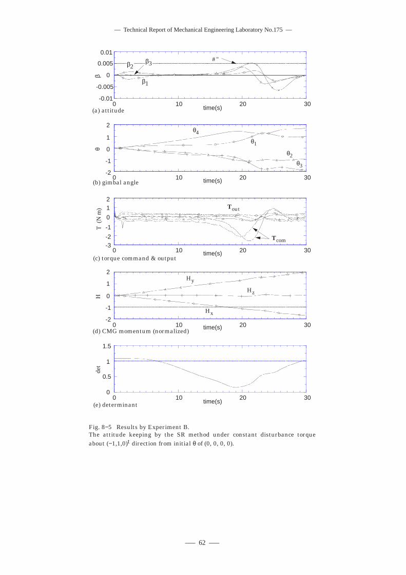
–– Technical Report of Mechanical Engineering Laboratory No.175 ––
––– 62 –––
Fig. 8−5 Results by Experiment B.The attitude keeping by the SR method under constant disturbance torque about (−1,1,0)t direction from initial θ of (0, 0, 0, 0).
AAAAAAAAAAAAAAAAAAAAAAAAAAAAAAAAAAAAAAAAAAAAAAAAAAAA
AAAA
AAAA
AAAA
AAAA
0
0.5
1
1.5
0 10 20 30
det
time(s)(e) determinant
AAAAAAAAAAAAAAAAAAAAAAAAAAAAAAAAAAAAAAAAAAAAAAAAAAAAAAAAAAAAAAAAA
AAAA
AAAA
AAAA
AAAA
-2
-1
0
1
2
0 10 20 30
H
time(s)(d) CMG momentum (normalized)
Hz
Hx
Hy
(b) gimbal angleAAAAAAAAAAAAAAAAAAAAAAAAAAAAAAAAAAAAAAAAAAAAAAAAAAAAAAAAAAAAAAAAA
AAAA
AAAA
AAAA
AAAA
-2
-1
0
1
2
0 10 20 30
θ
time(s)
θ1
θ2θ3
θ4
AAAAAAAAAAAAAAAAAAAAAAAAAAAAAAAAAAAAAAAAAAAAAAAAAAAAAAAAAAAAAAAAAAAAAAAAAAAAAA
AAAA
AAAA
AAAA
AAAA
-3-2
-1
0
12
0 10 20 30
T (
N m
)
time(s)(c) torque command & output
Tcom
Tout
AAAAAAAAAAAAAAAAAAAAAAAAAAAAAAAAAAAAAAAAAAAAAAAAAAAAAAAAAAAAAAAAA
AAAA
AAAA
AAAA
AAAA
-0.01
-0.005
0
0.005
0.01
0 10 20 30β
time(s)(a) attitude
β3β2
β1
BA
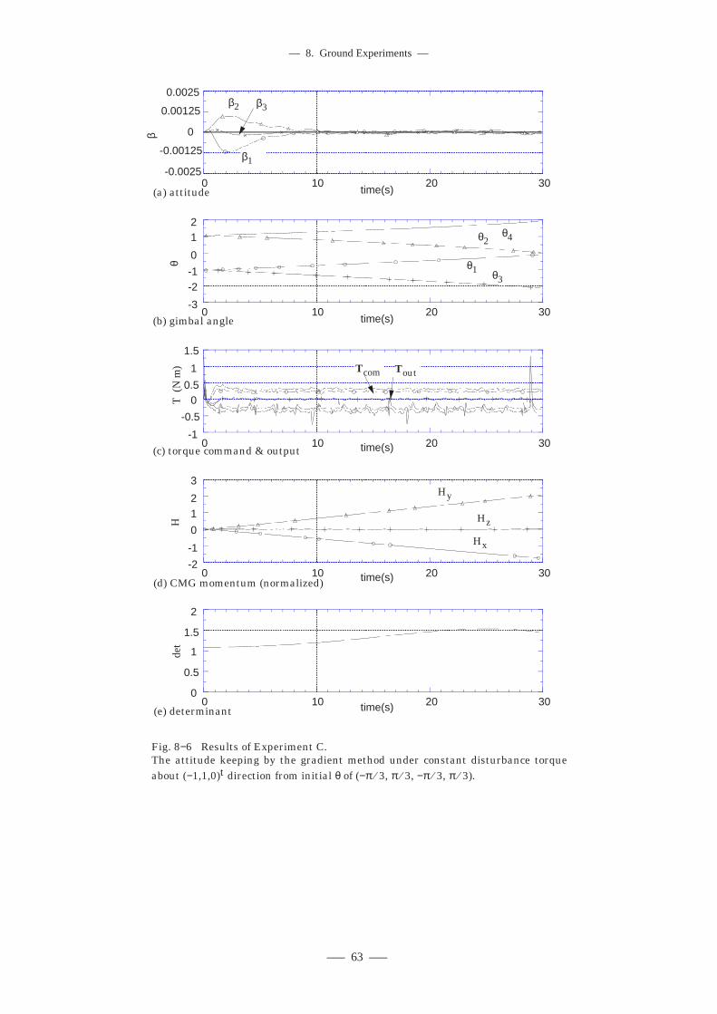
––– 63 –––
–– 8. Ground Experiments ––
Fig. 8−6 Results of Experiment C. The attitude keeping by the gradient method under constant disturbance torqueabout (−1,1,0)t direction from initial θ of (−π ⁄ 3, π ⁄ 3, −π ⁄ 3, π ⁄ 3).
AAAAAAAAAAAAAAAAAAAAAAAAAAAAAAAAAAAAAAAAAAAAAAAAAAAAAAAAAAAAAAAAA
AAAA
AAAA
AAAA
AAAA
0
0.5
1
1.5
2
0 10 20 30
det
time(s)(e) determinant
AAAAAAAAAAAAAAAAAAAAAAAAAAAAAAAAAAAAAAAAAAAAAAAAAAAAAAAAAAAAAAAAAAAAAAAAAAAAAA
AAAA
AAAA
AAAA
AAAA
-2
-1
0
12
3
0 10 20 30
H
time(s)(d) CMG momentum (normalized)
Hz
Hx
Hy
AAAAAAAAAAAAAAAAAAAAAAAAAAAAAAAAAAAAAAAAAAAAAAAAAAAAAAAAAAAAAAAAAAAAAAAAAAAAAA
AAAA
AAAA
AAAA
AAAA
-3
-2-1
0
12
0 10 20 30
θ
time(s)(b) gimbal angle
θ1
θ2
θ3
θ4
AAAAAAAAAAAAAAAAAAAAAAAAAAAAAAAAAAAAAAAAAAAAAAAAAAAAAAAAAAAAAAAAA
AAAA
AAAA
AAAA
AAAA
-0.0025
-0.00125
0
0.00125
0.0025
0 10 20 30
β
time(s)(a) attitude
β3β2
β1
AAAAAAAAAAAAAAAAAAAAAAAAAAAAAAAAAAAAAAAAAAAAAAAAAAAAAAAAAAAAAAAAAAAAAAAAAAAAAA
AAAA
AAAA
AAAA
AAAA
-1
-0.5
00.5
1
1.5
0 10 20 30
T (
N m
)
time(s)(c) torque command & output
Tcom Tout
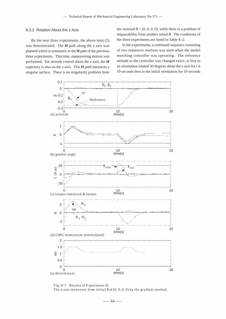
–– Technical Report of Mechanical Engineering Laboratory No.175 ––
––– 64 –––
8.3.2 Rotation About the z Axis
By the next three experiments, the above item (2)
was demonstrated. The H path along the z axis was
planned which is symmetric to the H path of the previousthree experiments. This time, maneuvering motion was
performed. For attitude control about the z axis, the Htrajectory is also on the z axis. This H path intersects asingular surface. There is no singularity problem from
the nominal θ = (0, 0, 0, 0), while there is a problem of
impassability from another initial θ. The conditions of
the three experiments are listed in Table 8–2.In the experiments, a command sequence consisting
of two maneuver motions was used when the model
matching controller was operating. The referenceattitude to the controller was changed twice, at first to
an orientation rotated 30 degrees about the z axis for t ≤10 seconds then to the initial orientation for 10 seconds
Fig. 8−7 Results of Experiment D. The z-axis maneuver from initial θ of (0, 0, 0, 0) by the gradient method.
AAAAAAAAAAAAAAAAAAAAAAAAAAAAAAAAAAAAAAAAAAAAAAAAAAAAAAAAAAAAAAAAA
AAAA
AAAA
AAAA
-1
0
1
0 10 20
θ
time(s)(b) gimbal angle
AAAAAAAAAAAAAAAAAAAAAAAAAAAAAAAAAAAAAAAAAAAAAAAAAAAAAAAAAAAAAAAAA
AAAA
AAAA
AAAA
0
0.5
1
1.5
2
0 10 20
det
time(s)(e) determinant
AAAAAAAAAAAAAAAAAAAAAAAAAAAAAAAAAAAAAAAAAAAAAAAAAAAAAAAAAAAAAAAAAAAAAAAAAAAAAA
AAAA
AAAA
AAAA
-0.3
-0.2
-0.1
0
0.1
0 10 20
β
time(s)(a) attitude
DA
Referenceβ3
β1, β2
AAAAAAAAAAAAAAAAAAAAAAAAAAAAAAAAAAAAAAAAAAAAAAAAAAAAAAAAAAAAAAAAA
AAAA
AAAA
AAAA
-2
0
2
0 10 20
H
time(s)(d) CMG momentum (normalized)
DB
Hz
Hx Hy
AAAAAAAAAAAAAAAAAAAAAAAAAAAAAAAAAAAAAAAAAAAAAAAAAAAAAAAAAAAAAAAAA
AAAA
AAAA
AAAA
-20
0
20
0 10 20
T (
N m
)
time(s)(c) torque command & output
Tcom Tout
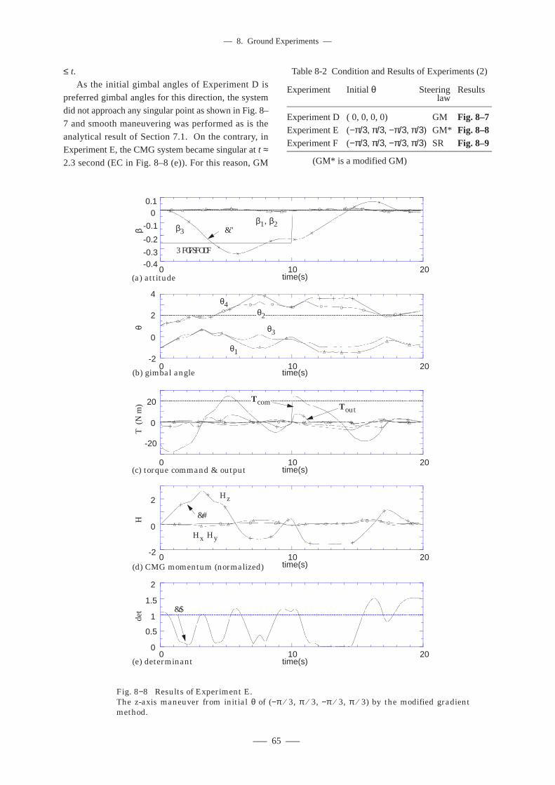
––– 65 –––
–– 8. Ground Experiments ––
Table 8-2 Condition and Results of Experiments (2)
Experiment Initial θ Steering Results law
——————————————————————Experiment D ( 0, 0, 0, 0) GM Fig. 8–7Experiment E (−π/3, π/3, −π/3, π/3) GM* Fig. 8–8Experiment F (−π/3, π/3, −π/3, π/3) SR Fig. 8–9—————————————————————— (GM* is a modified GM)
≤ t.
As the initial gimbal angles of Experiment D is
preferred gimbal angles for this direction, the systemdid not approach any singular point as shown in Fig. 8–
7 and smooth maneuvering was performed as is the
analytical result of Section 7.1. On the contrary, inExperiment E, the CMG system became singular at t ≈2.3 second (EC in Fig. 8–8 (e)). For this reason, GM
Fig. 8−8 Results of Experiment E. The z-axis maneuver from initial θ of (−π ⁄ 3, π ⁄ 3, −π ⁄ 3, π ⁄ 3) by the modified gradient method.
(e) determinantAAAAAAAAAAAAAAAAAAAAAAAAAAAAAAAAAAAAAAAAAAAAAAAAAAAAAAAAAAAAAAAAA
AAAA
AAAA
AAAA
0
0.5
1
1.5
2
0 10 20
det
time(s)
EC
(d) CMG momentum (normalized)
AAAAAAAAAAAAAAAAAAAAAAAAAAAAAAAAAAAAAAAAAAAAAAAAAAAA
AAAA
AAAA
AAAA
-2
0
2
0 10 20
H
time(s)
EB
Hz
Hx Hy
(a) attitudeAAAAAAAAAAAAAAAAAAAAAAAAAAAAAAAAAAAAAAAAAAAAAAAAAAAAAAAAAAAAAAAAAAAAAAAAAAAAAA
AAAA
AAAA
AAAA
-0.4-0.3
-0.2
-0.1
00.1
0 10 20
β
time(s)
EAβ3β1, β2
Reference
(b) gimbal angle
AAAAAAAAAAAAAAAAAAAAAAAAAAAAAAAAAAAAAAAAAAAAAAAAAAAA
AAAA
AAAA
AAAA
-2
0
2
4
0 10 20
θ
time(s)
θ1
θ2
θ3
θ4
(c) torque command & outputAAAAAAAAAAAAAAAAAAAAAAAAAAAAAAAAAAAAAAAAAAAAAAAAAAAAAAAAAAAAAAAAA
AAAA
AAAA
AAAA
-20
0
20
0 10 20
T (
N m
)
time(s)
ToutTcom
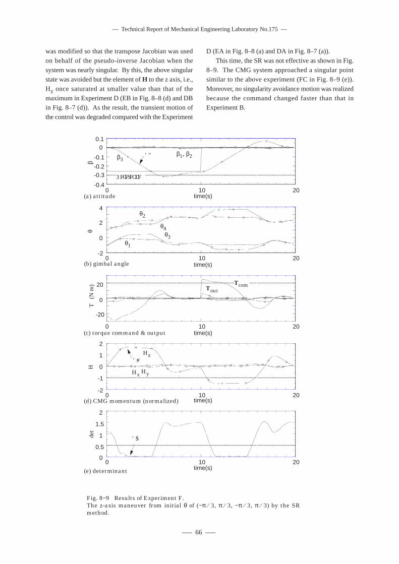
–– Technical Report of Mechanical Engineering Laboratory No.175 ––
––– 66 –––
was modified so that the transpose Jacobian was used
on behalf of the pseudo-inverse Jacobian when the
system was nearly singular. By this, the above singularstate was avoided but the element of H to the z axis, i.e.,
Hz once saturated at smaller value than that of the
maximum in Experiment D (EB in Fig. 8–8 (d) and DBin Fig. 8–7 (d)). As the result, the transient motion of
the control was degraded compared with the Experiment
D (EA in Fig. 8–8 (a) and DA in Fig. 8–7 (a)).
This time, the SR was not effective as shown in Fig.
8–9. The CMG system approached a singular pointsimilar to the above experiment (FC in Fig. 8–9 (e)).
Moreover, no singularity avoidance motion was realized
because the command changed faster than that inExperiment B.
Fig. 8−9 Results of Experiment F. The z-axis maneuver from initial θ of (−π ⁄ 3, π ⁄ 3, −π ⁄ 3, π ⁄ 3) by the SR method.
(e) determinantAAAAAAAAAAAAAAAAAAAAAAAAAAAAAAAAAAAAAAAAAAAAAAAAAAAAAAAAAAAAAAAAA
AAAA
AAAA
AAAA
0
0.5
1
1.5
2
0 10 20
det
time(s)
FC
(d) CMG momentum (normalized)AAAAAAAAAAAAAAAAAAAAAAAAAAAAAAAAAAAAAAAAAAAAAAAAAAAAAAAAAAAAAAAAA
AAAA
AAAA
AAAA
-2
-1
0
1
2
0 10 20
H
time(s)
FBHz
Hx Hy
(c) torque command & outputAAAAAAAAAAAAAAAAAAAAAAAAAAAAAAAAAAAAAAAAAAAAAAAAAAAAAAAAAAAAAAAAA
AAAA
AAAA
AAAA
-20
0
20
0 10 20
T
(N m
)
time(s)
TcomTout
(a) attitude
AAAAAAAAAAAAAAAAAAAAAAAAAAAAAAAAAAAAAAAAAAAAAAAAAAAAAAAAAAAAAAAAAAAAAAAAAAAAAA
AAAA
AAAA
AAAA
-0.4
-0.3-0.2
-0.1
00.1
0 10 20
β
time(s)
FAβ3β1, β2
Reference
(b) gimbal angleAAAAAAAAAAAAAAAAAAAAAAAAAAAAAAAAAAAAAAAAAAAAAAAAAAAA
AAAA
AAAA
AAAA
-2
0
2
4
0 10 20
θ
time(s)
θ1
θ2
θ3
θ4
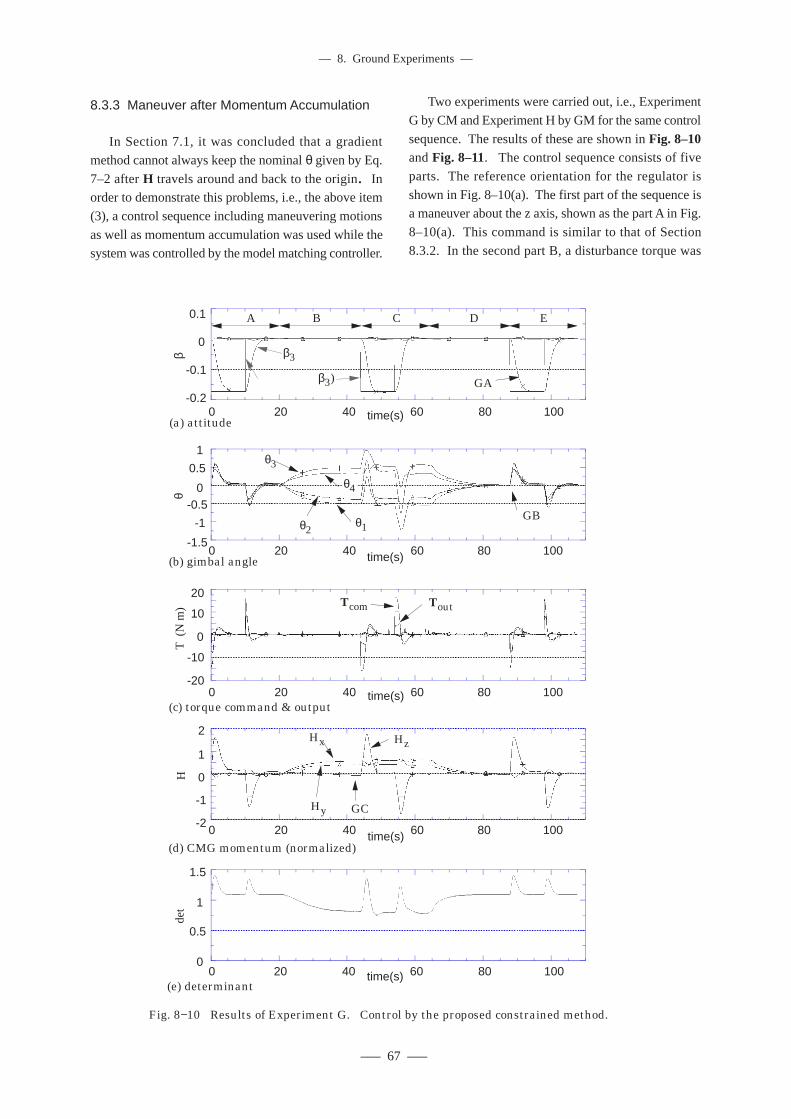
––– 67 –––
–– 8. Ground Experiments ––
8.3.3 Maneuver after Momentum Accumulation
In Section 7.1, it was concluded that a gradient
method cannot always keep the nominal θ given by Eq.
7–2 after H travels around and back to the origin. Inorder to demonstrate this problems, i.e., the above item
(3), a control sequence including maneuvering motions
as well as momentum accumulation was used while thesystem was controlled by the model matching controller.
Two experiments were carried out, i.e., Experiment
G by CM and Experiment H by GM for the same control
sequence. The results of these are shown in Fig. 8–10and Fig. 8–11. The control sequence consists of five
parts. The reference orientation for the regulator is
shown in Fig. 8–10(a). The first part of the sequence isa maneuver about the z axis, shown as the part A in Fig.
8–10(a). This command is similar to that of Section
8.3.2. In the second part B, a disturbance torque was
reference(
AAAAAAAAAAAAAAAAAAAAAAAAAAAAAAAAAAAAAAAAAAAAAAAAAAAAAAAAAAAAAAAAAAAAAAAAAAAAAA
AAAAAAAAAAAAAAAAAAAAAAAAAAAAAAAAAAAAAAAAAAAAAAAAAAAA
AAAA
AAAA
AAAA
AAAA
AAAA
AAAA
0
0.5
1
1.5
0 20 40 60 80 100(e) determinant
det
time(s)
Fig. 8−10 Results of Experiment G. Control by the proposed constrained method.
AAAAAAAAAAAAA
AAAAAAAAAAAAA
AAAA
AAAA
AAAA
AAAA
AAAA
AAAA
AAAAAAAAAAAAA
AAAAAAAAAAAAA
-20
-10
0
10
20
0 20 40 60 80 100(c) torque command & output
T (
N m
)
time(s)
Tcom Tout
AAAA
AAAA
AAAA
AAAA
AAAA
AAAA
-1.5
-1
-0.50
0.5
1
0 20 40 60 80 100(b) gimbal angle
θ
time(s)
GBθ1θ2
θ3
θ4
AAAAAAAAAAAAA
AAAAAAAAAAAAA
AAAA
AAAA
AAAA
AAAA
AAAA
AAAA
-2
-1
0
1
2
0 20 40 60 80 100
(d) CMG momentum (normalized)
H
time(s)
HzHx
Hy GC
(a) attitude
AAAAAAAAAAAAAAAAAAAAAAAAAAAAAAAAAAAAAAAAAAAAAAAAAAAA
AAAA
AAAA
AAAA
AAAA
AAAA
AAAA
-0.2
-0.1
0
0.1
0 20 40 60 80 100
β
time(s)
A B C D E
β3
reference(β3) GA
AAAAAAAAAAAAAAAAAAAAAAAAAAAAAAAAAAAAAAA
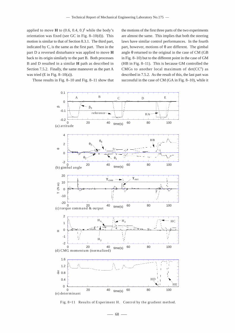
–– Technical Report of Mechanical Engineering Laboratory No.175 ––
––– 68 –––
applied to move H to (0.6, 0.4, 0.)t while the body’s
orientation was fixed (see GC in Fig. 8–10(d)). This
motion is similar to that of Section 8.3.1. The third part,indicated by C, is the same as the first part. Then in the
part D a reversed disturbance was applied to move Hback to its origin similarly to the part B. Both processesB and D resulted in a similar H path as described in
Section 7.5.2. Finally, the same maneuver as the part A
was tried (E in Fig. 8–10(a)).Those results in Fig. 8–10 and Fig. 8–11 show that
the motions of the first three parts of the two experiments
are almost the same. This implies that both the steering
laws have similar control performances. In the fourthpart, however, motions of θ are different. The gimbal
angle θ returned to the original in the case of CM (GB
in Fig. 8–10) but to the different point in the case of GM(HB in Fig. 8–11). This is because GM controlled the
CMGs to another local maximum of det(CCt) as
described in 7.5.2. As the result of this, the last part wassuccessful in the case of CM (GA in Fig. 8–10), while it
AAAAAAAAAAAAA
Fig. 8−11 Results of Experiment H. Control by the gradient method.
AAAAAAAAAAAAAAAAAAAAAAAAAAAAAAAAAAAAAAAAAAAAAAAAAAAAAAAAAAAAAAAAA
AAAA
AAAA
AAAA
AAAA
AAAA
AAAA
0
0.4
0.8
1.2
1.6
0 20 40 60 80 100
det
time(s)
HD
HE
(e) determinant
AAAAAAAAAAAAAAAAAAAAAAAAAA
AAAAAAAAAAAAAAAAAAAAAAAAAA
AAAA
AAAA
AAAA
AAAA
AAAA
AAAA
-20
-10
0
10
20
0 20 40 60 80 100
T (
N m
)
time(s)(c) torque command & output
TcomTout
AAAAAAAAAAAAAAAAAAAAAAAAAAAAAAAAAAAAAAAAAAAAAAAAAAAA
AAAA
AAAA
AAAA
AAAA
AAAA
AAAA
-2
0
2
4
0 20 40 60 80 100
θ
time(s)
HB
(b) gimbal angle
θ1θ2
θ3θ4
AAAAAAAAAAAAAAAAAAAAAAAAAAAAAAAAAAAAAAAAAAAAAAAAAAAA
AAAA
AAAA
AAAA
AAAA
AAAA
AAAA
-0.2
-0.1
0
0.1
0 20 40 60 80 100
β
time(s)
A B C D E
HA
(a) attitude
reference
β3
AAAAAAAAAAAAAAAAAAAAAAAAAAAAAAAAAAAAAAAAAAAAAAAAAAAAAAAAAAAAAAAAA
AAAA
AAAA
AAAA
AAAA
AAAA
AAAA
0 20 40 60 80 100
H
time(s)
HC
(d) CMG momentum (normalized)
HzHx
Hy-2
-1
0
1
2
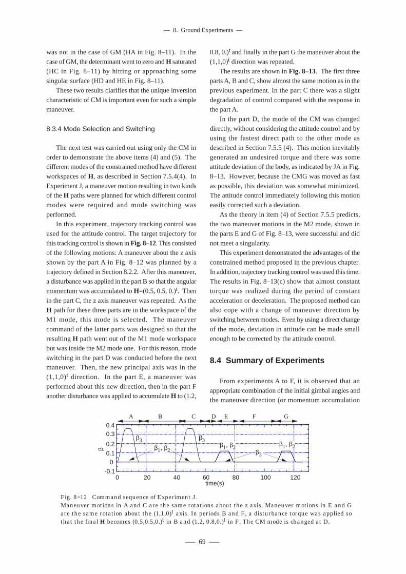
––– 69 –––
–– 8. Ground Experiments ––
was not in the case of GM (HA in Fig. 8–11). In the
case of GM, the determinant went to zero and H saturated
(HC in Fig. 8–11) by hitting or approaching somesingular surface (HD and HE in Fig. 8–11).
These two results clarifies that the unique inversion
characteristic of CM is important even for such a simplemaneuver.
8.3.4 Mode Selection and Switching
The next test was carried out using only the CM in
order to demonstrate the above items (4) and (5). Thedifferent modes of the constrained method have different
workspaces of H, as described in Section 7.5.4(4). In
Experiment J, a maneuver motion resulting in two kindsof the H paths were planned for which different control
modes were required and mode switching was
performed.In this experiment, trajectory tracking control was
used for the attitude control. The target trajectory for
this tracking control is shown in Fig. 8–12. This consistedof the following motions: A maneuver about the z axis
shown by the part A in Fig. 8–12 was planned by a
trajectory defined in Section 8.2.2. After this maneuver,a disturbance was applied in the part B so that the angular
momentum was accumulated to H=(0.5, 0.5, 0.)t. Then
in the part C, the z axis maneuver was repeated. As theH path for these three parts are in the workspace of the
M1 mode, this mode is selected. The maneuver
command of the latter parts was designed so that theresulting H path went out of the M1 mode workspace
but was inside the M2 mode one. For this reason, mode
switching in the part D was conducted before the nextmaneuver. Then, the new principal axis was in the
(1,1,0)t direction. In the part E, a maneuver was
performed about this new direction, then in the part Fanother disturbance was applied to accumulate H to (1.2,
0.8, 0.)t and finally in the part G the maneuver about the
(1,1,0)t direction was repeated.
The results are shown in Fig. 8–13. The first threeparts A, B and C, show almost the same motion as in the
previous experiment. In the part C there was a slight
degradation of control compared with the response inthe part A.
In the part D, the mode of the CM was changed
directly, without considering the attitude control and byusing the fastest direct path to the other mode as
described in Section 7.5.5 (4). This motion inevitably
generated an undesired torque and there was someattitude deviation of the body, as indicated by JA in Fig.
8–13. However, because the CMG was moved as fast
as possible, this deviation was somewhat minimized.The attitude control immediately following this motion
easily corrected such a deviation.
As the theory in item (4) of Section 7.5.5 predicts,the two maneuver motions in the M2 mode, shown in
the parts E and G of Fig. 8–13, were successful and did
not meet a singularity.This experiment demonstrated the advantages of the
constrained method proposed in the previous chapter.
In addition, trajectory tracking control was used this time.The results in Fig. 8–13(c) show that almost constant
torque was realized during the period of constant
acceleration or deceleration. The proposed method canalso cope with a change of maneuver direction by
switching between modes. Even by using a direct change
of the mode, deviation in attitude can be made smallenough to be corrected by the attitude control.
8.4 Summary of Experiments
From experiments A to F, it is observed that an
appropriate combination of the initial gimbal angles andthe maneuver direction (or momentum accumulation
Fig. 8−12 Command sequence of Experiment J.Maneuver motions in A and C are the same rotations about the z axis. Maneuver motions in E and G are the same rotation about the (1,1,0)t axis. In periods B and F, a disturbance torque was applied so that the final H becomes (0.5,0.5,0.)t in B and (1.2, 0.8,0.)t in F. The CM mode is changed at D.
AAAAAAAAAAAAAAAAAAAAAAAAAAAAAAAAAAAAAAAAAAAAAAAAAAAAAAAAAAAAAAAAAAAAAAAAAAAAAAAAAAAA
AAAAAAAA
AAAA
AAAA
AAAA
AAAA
AAAA
AAAA
-0.1
00.1
0.2
0.30.4
0 20 40 60 80 100 120
β
time(s)
A B C D E F G
β3 β3β1, β2 β1, β2β1, β2 β3
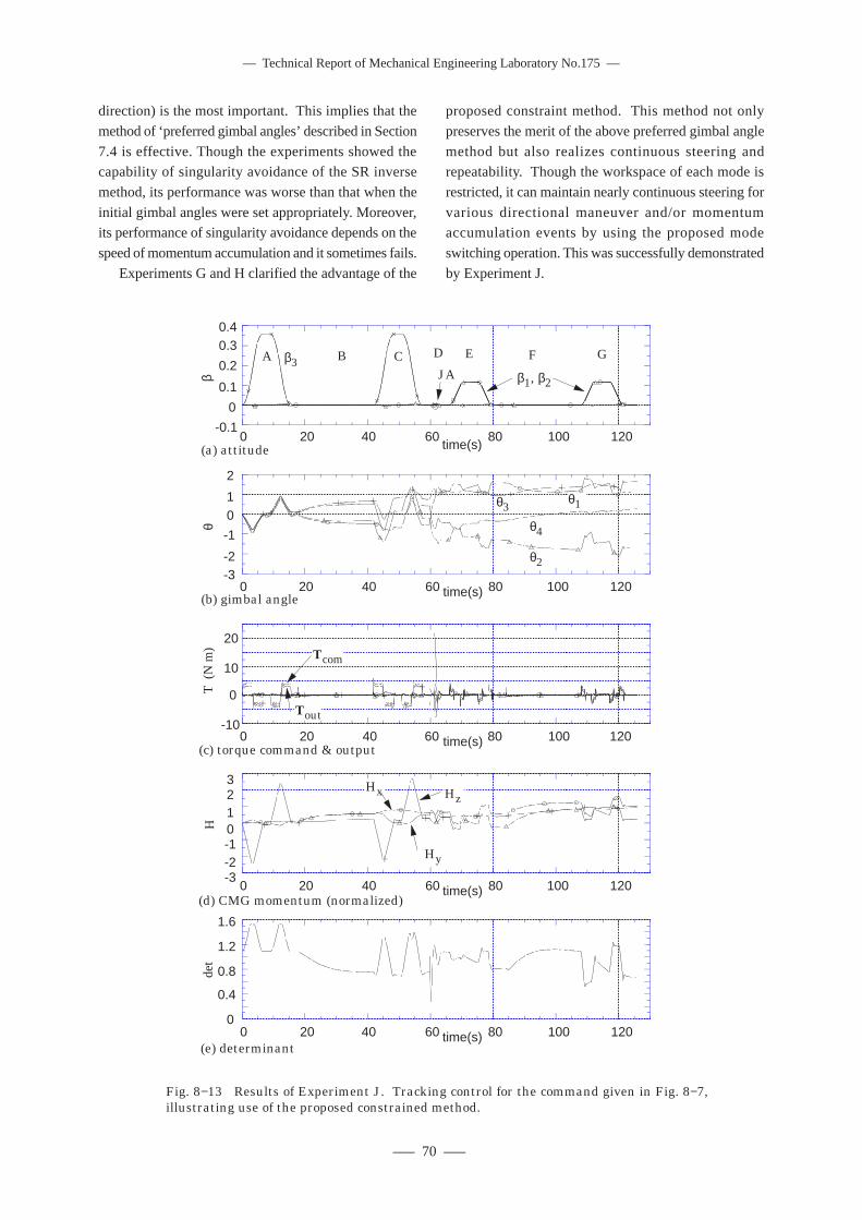
–– Technical Report of Mechanical Engineering Laboratory No.175 ––
––– 70 –––
direction) is the most important. This implies that the
method of ‘preferred gimbal angles’ described in Section
7.4 is effective. Though the experiments showed thecapability of singularity avoidance of the SR inverse
method, its performance was worse than that when the
initial gimbal angles were set appropriately. Moreover,its performance of singularity avoidance depends on the
speed of momentum accumulation and it sometimes fails.
Experiments G and H clarified the advantage of the
proposed constraint method. This method not only
preserves the merit of the above preferred gimbal angle
method but also realizes continuous steering andrepeatability. Though the workspace of each mode is
restricted, it can maintain nearly continuous steering for
various directional maneuver and/or momentumaccumulation events by using the proposed mode
switching operation. This was successfully demonstrated
by Experiment J.
Fig. 8−13 Results of Experiment J. Tracking control for the command given in Fig. 8−7, illustrating use of the proposed constrained method.
AAAAAAAAAAAAAAAAAAAAAAAAAAAAAAAAAAAAAAAAAAAAAAAAAAAAAAAAAAAAAAAAA
AAAA
AAAA
AAAA
AAAA
AAAA
AAAA
AAAA
0
0.4
0.8
1.2
1.6
0 20 40 60 80 100 120
det
time(s)(e) determinant
(b) gimbal angleAAAAAAAAAAAAAAAAAAAAAAAAAAAAAAAAAAAAAAAAAAAAAAAAAAAAAAAAAAAAAAAAAAAAAAAAAAAAAA
AAAA
AAAA
AAAA
AAAA
AAAA
AAAA
AAAA
-3-2
-1
01
2
0 20 40 60 80 100 120
θ
time(s)
θ1
θ2
θ3
θ4
(a) attitude
AAAAAAAAAAAAAAAAAAAAAAAAAAAAAAAAAAAAAAAAAAAAAAAAAAAAAAAAAAAAAAAAAAAAAAAAAAAAAA
AAAA
AAAA
AAAA
AAAA
AAAA
AAAA
AAAA
-0.1
0
0.1
0.2
0.30.4
0 20 40 60 80 100 120
β
time(s)
A B C D E F G
JAβ3
β1, β2
(d) CMG momentum (normalized)AAAAAAAAAAAAAAAAAAAAAAAAAAAAAAAAAAAAAAAAAAAAAAAAAAAAAAAAAAAAAAAAAAAAAAAAAAAAAAAAAAAAAAAAAAA
AAAA
AAAA
AAAA
AAAA
AAAA
AAAA
AAAA
-3-2-10123
0 20 40 60 80 100 120
H
time(s)
HzHx
Hy
(c) torque command & output
AAAAAAAAAAAAAAAAAAAAAAAAAAAAAAAAAAAAAAAAAAAAAAAAAAAAAAAAAAAAAAAAAAAAAAAAAAAAAAAAAAAAAAAAAAAAAAAAAAAAAAAA
AAAA
AAAA
AAAA
AAAA
AAAA
AAAA
AAAA
-10
0
10
20
0 20 40 60 80 100 120
T (
N m
)
time(s)
Tcom
Tout
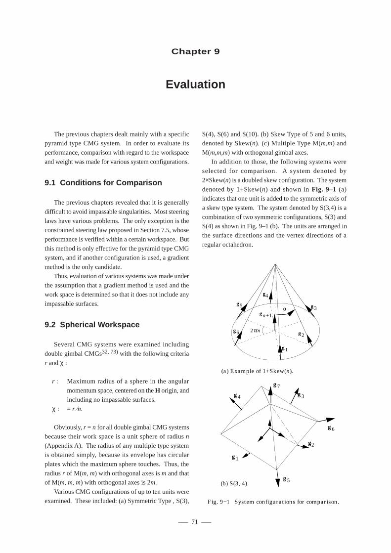
––– 71 –––
–– 9. Evaluation ––
The previous chapters dealt mainly with a specificpyramid type CMG system. In order to evaluate its
performance, comparison with regard to the workspace
and weight was made for various system configurations.
9.1 Conditions for Comparison
The previous chapters revealed that it is generally
difficult to avoid impassable singularities. Most steering
laws have various problems. The only exception is theconstrained steering law proposed in Section 7.5, whose
performance is verified within a certain workspace. But
this method is only effective for the pyramid type CMGsystem, and if another configuration is used, a gradient
method is the only candidate.
Thus, evaluation of various systems was made underthe assumption that a gradient method is used and the
work space is determined so that it does not include any
impassable surfaces.
9.2 Spherical Workspace
Several CMG systems were examined including
double gimbal CMGs32, 73) with the following criteria
r and χ :
r : Maximum radius of a sphere in the angular
momentum space, centered on the H origin, andincluding no impassable surfaces.
χ : = r ⁄n.
Obviously, r = n for all double gimbal CMG systems
because their work space is a unit sphere of radius n
(Appendix A). The radius of any multiple type systemis obtained simply, because its envelope has circular
plates which the maximum sphere touches. Thus, the
radius r of M(m, m) with orthogonal axes is m and thatof M(m, m, m) with orthogonal axes is 2m.
Various CMG configurations of up to ten units were
examined. These included: (a) Symmetric Type , S(3),
S(4), S(6) and S(10). (b) Skew Type of 5 and 6 units,denoted by Skew(n). (c) Multiple Type M(m,m) and
M(m,m,m) with orthogonal gimbal axes.
In addition to those, the following systems wereselected for comparison. A system denoted by
2×Skew(n) is a doubled skew configuration. The system
denoted by 1+Skew(n) and shown in Fig. 9–1 (a)indicates that one unit is added to the symmetric axis of
a skew type system. The system denoted by S(3,4) is a
combination of two symmetric configurations, S(3) andS(4) as shown in Fig. 9–1 (b). The units are arranged in
the surface directions and the vertex directions of a
regular octahedron.
Chapter 9
Evaluation
g1
g2
g3
g4g5
g6
α
2π⁄n
gn+1
(a) Example of 1+Skew(n).
Fig. 9−1 System configurations for comparison.
g2
g3g4
g1
g5
g6
g7
(b) S(3, 4).
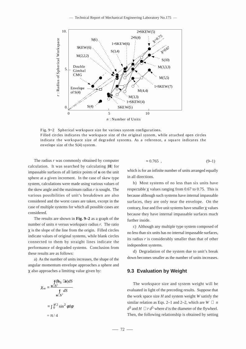
–– Technical Report of Mechanical Engineering Laboratory No.175 ––
––– 72 –––
The radius r was commonly obtained by computer
calculation. It was searched by calculating |H | forimpassable surfaces of all lattice points of u on the unit
sphere at a given increment. In the case of skew type
system, calculations were made using various values ofthe skew angle and the maximum radius r is sought. The
various possibilities of unit’s breakdown are also
considered and the worst cases are taken, except in thecase of multiple systems for which all possible cases are
considered.
The results are shown in Fig. 9–2 as a graph of thenumber of units n versus workspace radius r. The ratio
χ is the slope of the line from the origin. Filled circles
indicate values of original systems, while blank circlesconnected to them by straight lines indicate the
performance of degraded systems. Conclusion from
these results are as follows:a) As the number of units increases, the shape of the
angular momentum envelope approaches a sphere and
χ also approaches a limiting value given by:
χ∞∈
∈
=∫ ⋅
∫
( )h uu
u
SS
S
2
2
dS
dS
= ∫ ⁄0
2 2π φ φsin d
= π / 4
≈ 0.765 , (9–1)
which is for an infinite number of units arranged equally
in all directions.
b) Most systems of no less than six units have
respectable χ values ranging from 0.67 to 0.75. This is
because although such systems have internal impassable
surfaces, they are only near the envelope. On the
contrary, four and five unit systems have smaller χ values
because they have internal impassable surfaces much
further inside.
c) Although any multiple type system composed of
no less than six units has no internal impassable surfaces,
its radius r is considerably smaller than that of other
independent systems.
d) Degradation of the system due to unit’s break
down becomes smaller as the number of units increases.
9.3 Evaluation by Weight
The workspace size and system weight will be
evaluated in light of the preceding results. Suppose that
the work space size H and system weight W satisfy the
similar relation as Eqs. 2–1 and 2–2, which are W ∝ n
d3 and H ∝ r d5 where d is the diameter of the flywheel.
Then, the following relationship is obtained by setting
Fig. 9−2 Spherical workspace size for various system configurations.Filled circles indicates the workspace size of the original system, while attached open circles indicate the workspace size of degraded systems. As a reference, a square indicates the envelope size of the S(4) system.
M(5,5)
M(4,4)
S(4)1+SKEW(4)
SKEW(5)
S(6)
SKEW(6)
M(2,2,2)S(3,4)
1+SKEW(6)
2×S(4)
1+SKEW(7)
2×SKEW(5)
S(10)
M(3,3,3)
χ=0.75
χ=0.67
5.
0.
0 5 10
M(3,3)
10.
n : Number of Units
r : R
adiu
s of
Sph
eric
al W
orks
pace
Double Gimbal CMG
Envelope of S(4)
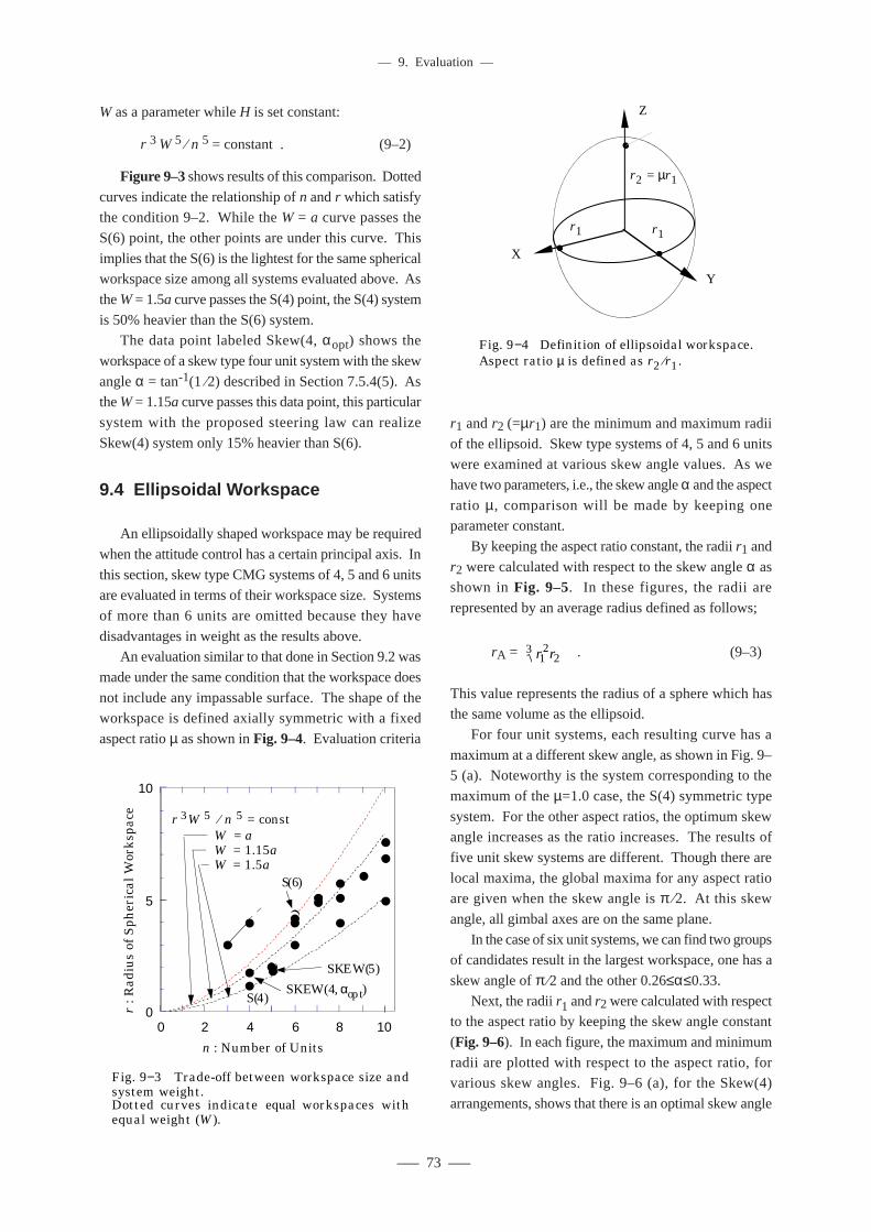
––– 73 –––
–– 9. Evaluation ––
W as a parameter while H is set constant:
r 3 W 5 ⁄ n 5 = constant . (9–2)
Figure 9–3 shows results of this comparison. Dotted
curves indicate the relationship of n and r which satisfythe condition 9–2. While the W = a curve passes the
S(6) point, the other points are under this curve. This
implies that the S(6) is the lightest for the same sphericalworkspace size among all systems evaluated above. As
the W = 1.5a curve passes the S(4) point, the S(4) system
is 50% heavier than the S(6) system.The data point labeled Skew(4, αopt) shows the
workspace of a skew type four unit system with the skew
angle α = tan-1(1 ⁄2) described in Section 7.5.4(5). Asthe W = 1.15a curve passes this data point, this particular
system with the proposed steering law can realize
Skew(4) system only 15% heavier than S(6).
9.4 Ellipsoidal Workspace
An ellipsoidally shaped workspace may be required
when the attitude control has a certain principal axis. In
this section, skew type CMG systems of 4, 5 and 6 unitsare evaluated in terms of their workspace size. Systems
of more than 6 units are omitted because they have
disadvantages in weight as the results above.An evaluation similar to that done in Section 9.2 was
made under the same condition that the workspace does
not include any impassable surface. The shape of theworkspace is defined axially symmetric with a fixed
aspect ratio µ as shown in Fig. 9–4. Evaluation criteria
r1 and r2 (=µr1) are the minimum and maximum radii
of the ellipsoid. Skew type systems of 4, 5 and 6 unitswere examined at various skew angle values. As we
have two parameters, i.e., the skew angle α and the aspect
ratio µ, comparison will be made by keeping oneparameter constant.
By keeping the aspect ratio constant, the radii r1 and
r2 were calculated with respect to the skew angle α asshown in Fig. 9–5. In these figures, the radii are
represented by an average radius defined as follows;
rA = r r12
23 . (9–3)
This value represents the radius of a sphere which hasthe same volume as the ellipsoid.
For four unit systems, each resulting curve has a
maximum at a different skew angle, as shown in Fig. 9–5 (a). Noteworthy is the system corresponding to the
maximum of the µ=1.0 case, the S(4) symmetric type
system. For the other aspect ratios, the optimum skewangle increases as the ratio increases. The results of
five unit skew systems are different. Though there are
local maxima, the global maxima for any aspect ratioare given when the skew angle is π ⁄2. At this skew
angle, all gimbal axes are on the same plane.
In the case of six unit systems, we can find two groupsof candidates result in the largest workspace, one has a
skew angle of π ⁄2 and the other 0.26≤α≤0.33.
Next, the radii r1 and r2 were calculated with respectto the aspect ratio by keeping the skew angle constant
(Fig. 9–6). In each figure, the maximum and minimum
radii are plotted with respect to the aspect ratio, forvarious skew angles. Fig. 9–6 (a), for the Skew(4)
arrangements, shows that there is an optimal skew angle
Fig. 9−4 Definition of ellipsoidal workspace.Aspect ratio µ is defined as r2 ⁄r1.
r1 r1
r2 = µr1
X
Y
Z
S(6)
0
5
10
0 2 4 6 8 10
n : Number of Units
r : R
adiu
s of
Sph
eric
al W
orks
pace r 3W 5 ⁄ n 5 = const
W = aW = 1.15aW = 1.5a
S(4)
SKEW(5)
SKEW(4, αopt)
Fig. 9−3 Trade-off between workspace size and system weight.Dotted curves indicate equal workspaces with equal weight (W).
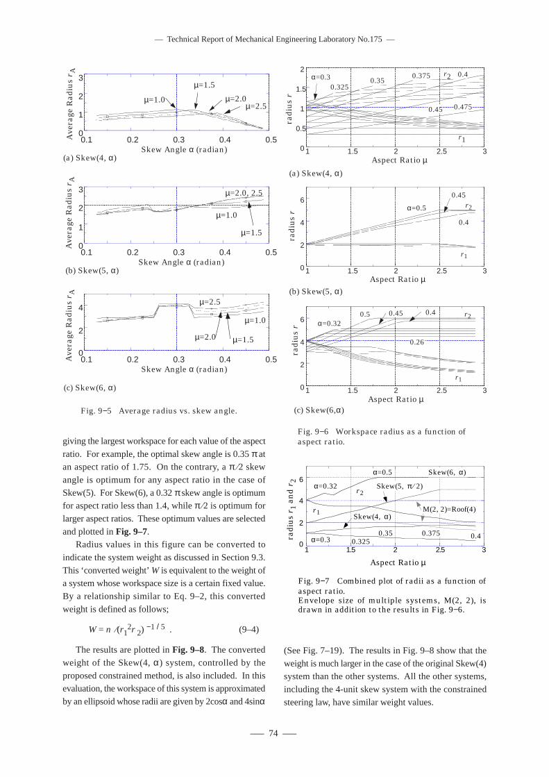
–– Technical Report of Mechanical Engineering Laboratory No.175 ––
––– 74 –––
giving the largest workspace for each value of the aspect
ratio. For example, the optimal skew angle is 0.35 π atan aspect ratio of 1.75. On the contrary, a π ⁄2 skew
angle is optimum for any aspect ratio in the case of
Skew(5). For Skew(6), a 0.32 π skew angle is optimumfor aspect ratio less than 1.4, while π ⁄2 is optimum for
larger aspect ratios. These optimum values are selected
and plotted in Fig. 9–7.Radius values in this figure can be converted to
indicate the system weight as discussed in Section 9.3.
This ‘converted weight’ W is equivalent to the weight ofa system whose workspace size is a certain fixed value.
By a relationship similar to Eq. 9–2, this converted
weight is defined as follows;
W = n ⁄(r12r
2) −1 / 5 . (9–4)
The results are plotted in Fig. 9–8. The converted
weight of the Skew(4, α) system, controlled by the
proposed constrained method, is also included. In thisevaluation, the workspace of this system is approximated
by an ellipsoid whose radii are given by 2cosα and 4sinα
r1
Fig. 9−6 Workspace radius as a function of aspect ratio.
(a) Skew(4, α)
radi
us
r
Aspect Ratio µAAAAAAAAAAAAAAAAAAAAAAAAAAAAAAAAAAAAAAAAAAAAA
AAAAA
AAAAA
AAAAA
AAAAA
AAAAA
0
0.5
1
1.5
2
1 1.5 2 2.5 3
0.3250.35
0.375 0.4
0.45
α=0.3
0.475
r2
(b) Skew(5, α)AAAAAAAAAAAAAAAAAA
AAAAAAAAAAAAAAAAAA
AAAAA
AAAAA
AAAAA
AAAAA
AAAAA
0
2
4
6
1 1.5 2 2.5 3
0.4
α=0.5
0.45
radi
us
rAspect Ratio µ
r2
r1
(c) Skew(6,α)
AAAAAAAAAAAAAAAAAAAAAAAAAAAAAAAAAAAA
AAAAA
AAAAA
AAAAA
AAAAA
AAAAA
0
2
4
6
1 1.5 2 2.5 3
0.40.5 0.45α=0.32
0.26
radi
us
r
Aspect Ratio µ
r2
r1
(See Fig. 7–19). The results in Fig. 9–8 show that the
weight is much larger in the case of the original Skew(4)system than the other systems. All the other systems,
including the 4-unit skew system with the constrained
steering law, have similar weight values.
AAAAAAAAAAAAAAAAAAAAAAAAAAAAAAAAAAAA
AAA
AAA
AAA
AAA
AAA
0
1
2
3
0.1 0.2 0.3 0.4 0.5Ave
rage
Rad
ius
r A
Skew Angle α (radian)
µ=2.0µ=1.0
µ=1.5
µ=2.5
(a) Skew(4, α)
Fig. 9−5 Average radius vs. skew angle.
AAAAAAAAAAAAAAAAAAAAAAAAAAAAAAAAAAAAAAAAAAAAA
AAAA
AAAA
AAAA
AAAA
AAAA
0
1
2
3
0.1 0.2 0.3 0.4 0.5Skew Angle α (radian)
µ=2.0, 2.5
µ=1.0
µ=1.5
(b) Skew(5, α)
Ave
rage
Rad
ius
r A
AAAAAAAAA
AAAAAAAAAAAAAAAAAA
AAAA
AAAA
AAAA
AAAA
AAAA
0
2
4
0.1 0.2 0.3 0.4 0.5Skew Angle α (radian)
µ=2.5
µ=1.0
µ=2.0 µ=1.5
(c) Skew(6, α)
Ave
rage
Rad
ius
r A
Fig. 9−7 Combined plot of radii as a function of aspect ratio.Envelope size of multiple systems, M(2, 2), is drawn in addition to the results in Fig. 9−6.
0
2
4
6
1 1.5 2 2.5 3
α=0.5
α=0.32
radi
us
r 1 a
nd
r 2
Aspect Ratio µ
0.3250.35 0.375 0.4α=0.3
r1
Skew(5, π ⁄ 2)
Skew(4, α)M(2, 2)=Roof(4)
Skew(6, α)
r2
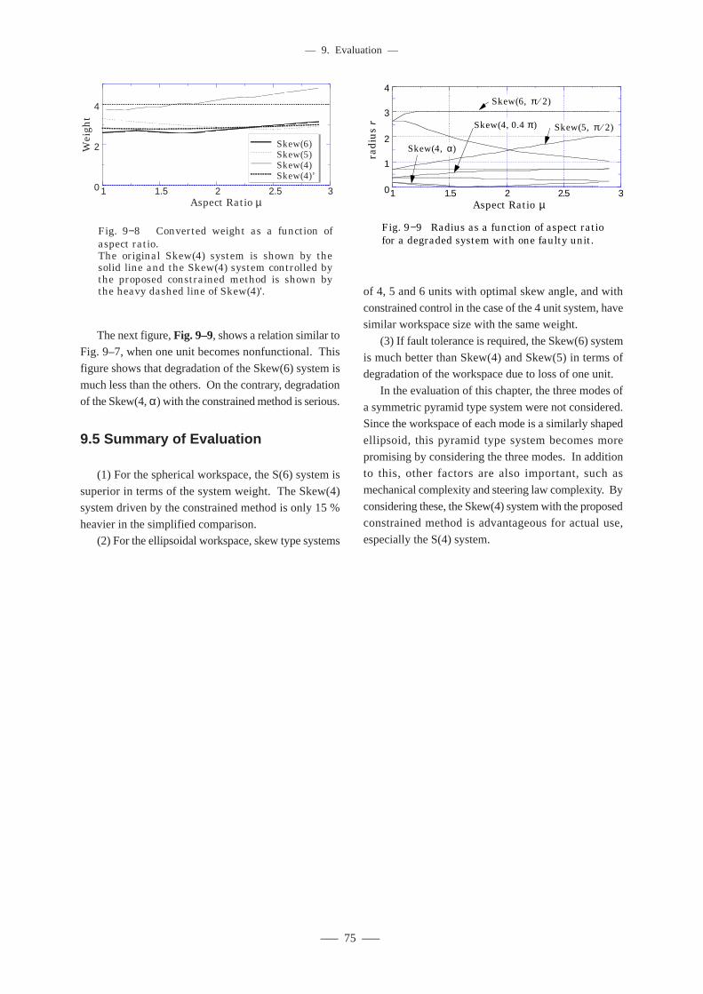
––– 75 –––
–– 9. Evaluation ––
The next figure, Fig. 9–9, shows a relation similar toFig. 9–7, when one unit becomes nonfunctional. This
figure shows that degradation of the Skew(6) system is
much less than the others. On the contrary, degradationof the Skew(4, α) with the constrained method is serious.
9.5 Summary of Evaluation
(1) For the spherical workspace, the S(6) system is
superior in terms of the system weight. The Skew(4)system driven by the constrained method is only 15 %
heavier in the simplified comparison.(2) For the ellipsoidal workspace, skew type systems
AAAAAAAAAA
AAAAAAAAAAAAAAAAAAAA
AAAAA
AAAAA
AAAAA
AAAAA
AAAAA
0
2
4
1 1.5 2 2.5 3
Wei
ght
Aspect Ratio µ
Fig. 9−8 Converted weight as a function of aspect ratio.The original Skew(4) system is shown by the solid line and the Skew(4) system controlled by the proposed constrained method is shown by the heavy dashed line of Skew(4)'.
Skew(6)Skew(5)Skew(4)Skew(4)’
of 4, 5 and 6 units with optimal skew angle, and with
constrained control in the case of the 4 unit system, havesimilar workspace size with the same weight.
(3) If fault tolerance is required, the Skew(6) system
is much better than Skew(4) and Skew(5) in terms ofdegradation of the workspace due to loss of one unit.
In the evaluation of this chapter, the three modes of
a symmetric pyramid type system were not considered.Since the workspace of each mode is a similarly shaped
ellipsoid, this pyramid type system becomes more
promising by considering the three modes. In additionto this, other factors are also important, such as
mechanical complexity and steering law complexity. By
considering these, the Skew(4) system with the proposedconstrained method is advantageous for actual use,
especially the S(4) system.
Fig. 9−9 Radius as a function of aspect ratio for a degraded system with one faulty unit.
radi
us
r
Aspect Ratio µ0
1
2
3
4
1 1.5 2 2.5 3
Skew(6, π ⁄ 2)
Skew(4, 0.4 π )
Skew(4, α)
Skew(5, π ⁄ 2)

–– Technical Report of Mechanical Engineering Laboratory No.175 ––
––– 76 –––
––– 77 –––
–– 9. Evaluation ––
In this paper, the control of a single gimbal CMGsystem has been investigated, with emphasis on the
symmetric pyramid type. Specifically, the singularity
problems have been examined using geometric theoriesand computer calculations. The “global” problem of the
pyramid type system has been clarified, and a new
steering law approach has been proposed and verifiedusing ground experiments.
In Chapter 2, single gimbal CMGs were described in
comparison with double gimbal CMGs and reactionwheels. Then in Chapter 3, an analytical formulation of
general single gimbal CMGs was presented.
In Chapter 4, the singularity problem was described.Methods for obtaining singular surfaces, especially the
envelope, were presented. The passability of a singular
surface was defined. Then, examples of some impassablesurfaces of various CMG systems were given. The
results showed that impassable singularity is a serious
problem for the steering law of 4 and 5 unit CMGsystems. In Chapter 5, continuous steering under the
existence of an impassable singular surface has been
generally examined by using a topological study. Amethod to overcome some types of impassable
singularities were described in a geometric manner.
Some example conditions were presented in which nosteering law can realize continuous motion.
In Chapter 6, the symmetric pyramid type CMG
system was defined. Analytical results includingsymmetry and singular surface structure were presented.
Chapter 7 clarified the global steering problem that
continuous real-time steering cannot be realized overmost of the workspace. By the consequences of this
and by geometric theories, typical steering laws were
evaluated. This evaluation showed that steering lawexactness is the most important. An alternative steering
law was proposed which maintains exactness but which
is valid in a restricted workspace. Then in Chapter 8,this proposed method was evaluated using ground
experiments. First, the problems described in Chapter 7
were demonstrated. Then, the proposed method andother steering laws were tested using some attitude
control sequences. The performance of the proposed
method was verified, especially for a realistic sequenceincluding maneuvering and pointing under a specified
directional disturbance.
In Chapter 9, a pyramid type system with the proposedsteering law was compared with other types of CMG
systems. Evaluation according to workspace size
showed that the symmetric six unit system was superiorin terms of weight. However, the proposed method, with
spherically shaped workspace, showed significant
improvement. Moreover, it was shown that theworkspace size was almost equal to that of the five or
six unit skew system when an ellipsoidal workspace is
considered. Because of this result and the fact that asymmetric pyramid type system has three modes, as well
as mechanical and steering law simplicity, it was
concluded that the pyramid type CMG system with theproposed steering law would be an ideal candidate for
three axis attitude control.
This paper does not include studies of more realisticattitude control problems, which should be investigated
in consideration with the results of this paper. Evaluation
may require more detailed characteristics with regard tomission requirement, disturbance profiles and unloading
torquer specifications.
Chapter 10
Conclusions

–– Technical Report of Mechanical Engineering Laboratory No.175 ––
––– 78 –––
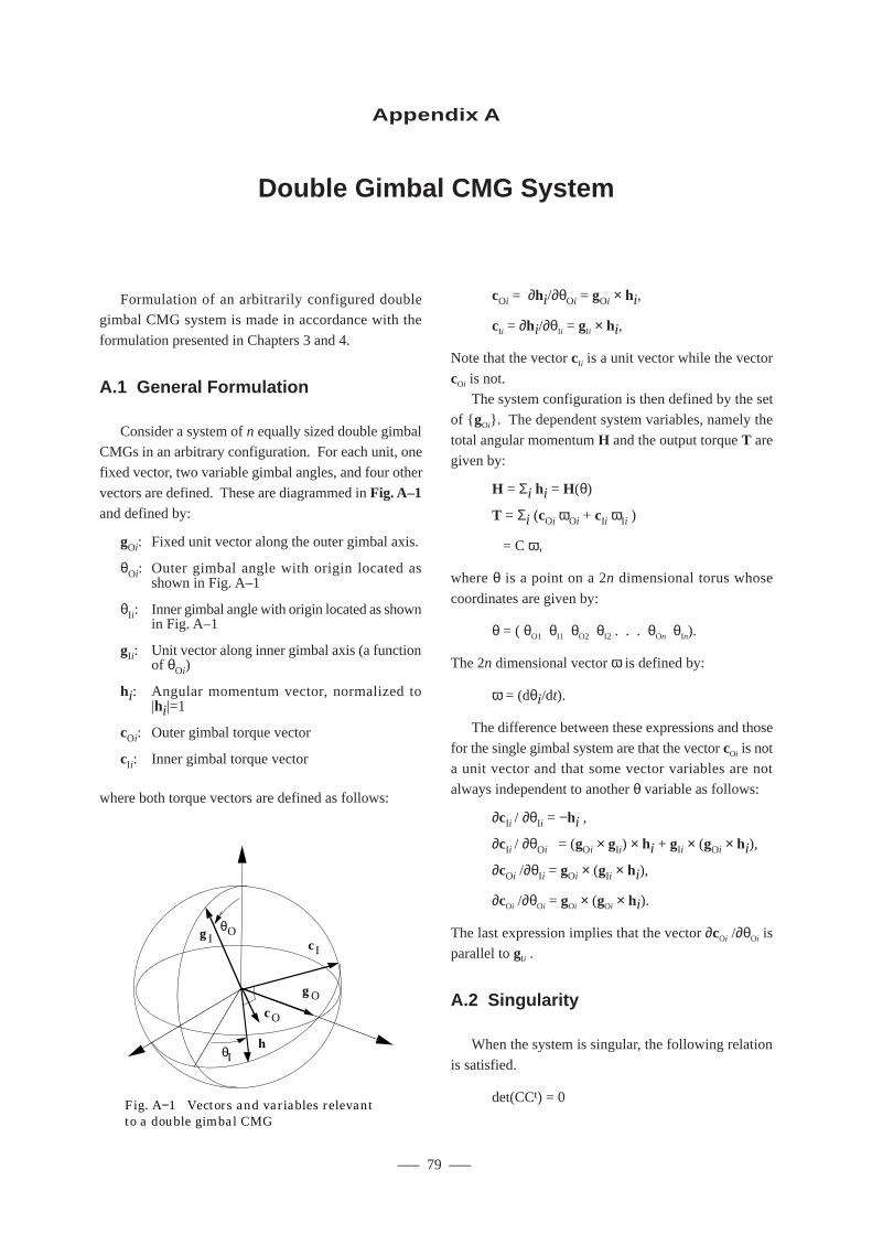
––– 79 –––
Formulation of an arbitrarily configured doublegimbal CMG system is made in accordance with the
formulation presented in Chapters 3 and 4.
A.1 General Formulation
Consider a system of n equally sized double gimbalCMGs in an arbitrary configuration. For each unit, one
fixed vector, two variable gimbal angles, and four other
vectors are defined. These are diagrammed in Fig. A–1and defined by:
gOi: Fixed unit vector along the outer gimbal axis.
θOi: Outer gimbal angle with origin located asshown in Fig. A–1
θIi: Inner gimbal angle with origin located as shownin Fig. A–1
gIi: Unit vector along inner gimbal axis (a functionof θOi)
hi: Angular momentum vector, normalized to|hi|=1
cOi: Outer gimbal torque vector
cIi: Inner gimbal torque vector
where both torque vectors are defined as follows:
cOi = ∂hi/∂θOi = gOi × hi,
cIi = ∂hi/∂θIi = gIi × hi,
Note that the vector cI i is a unit vector while the vector
cOi is not.The system configuration is then defined by the set
of {gOi}. The dependent system variables, namely the
total angular momentum H and the output torque T aregiven by:
H = Σi hi = H(θ)
T = Σi (cOi ωOi + cIi ωIi )
= C ω,
where θ is a point on a 2n dimensional torus whose
coordinates are given by:
θ = ( θO1 θI1 θO2 θI2 . . . θOn θIn).
The 2n dimensional vector ω is defined by:
ω = (dθi/dt).
The difference between these expressions and those
for the single gimbal system are that the vector cOi is nota unit vector and that some vector variables are not
always independent to another θ variable as follows:
∂cIi / ∂θIi = −hi ,
∂cIi / ∂θOi = (gOi × gIi) × hi + gIi × (gOi × hi),
∂cOi /∂θIi = gOi × (gIi × hi),
∂cOi /∂θOi = gOi × (gOi × hi).
The last expression implies that the vector ∂cOi /∂θOi isparallel to gIi .
A.2 Singularity
When the system is singular, the following relation
is satisfied.
det(CCt) = 0
Appendix A
Double Gimbal CMG System
Fig. A−1 Vectors and variables relevant to a double gimbal CMG
gI
gO
cI
h
cO
θO
θI

–– Technical Report of Mechanical Engineering Laboratory No.175 ––
––– 80 –––
Geometric comprehension of this fact is easier than the
case of a single gimbal system. Since both torque vectors
are orthogonal to each other and to h, a singular vectoru is determined as u parallels h. An exception arises
when the vector hi is parallel to the vector gOi, where cIi
is a zero vector. Thus, there are four possible conditionsof singularity for each unit when u is specified:
(a) hi = εi u, where εi=1 or −1
(b) hi = εi gOi, and (gIi × gOi).u = 0,
where εi=1 or −1.
These are drawn in Fig. A–2. Condition (b) is called
‘gimbal lock’ because such a unit looses one degree offreedom autonomously.
Because the domain of u is a unit sphere, the total
angular momentum H forms a number of spheres inaccordance with the set of εi.
A.3 Steering Law and Null Motion
Any steering law has the same expression as in Eq.
3–9. When the system is singular, some null motionsare easily obtained as follows. Referring back to the
previous section, suppose further that some unit is in
condition (b), then any dθOi results in the same H. This
implies that outer gimbal motion of this unit alone is anull motion. When there are two units both in condition
(a) but different signs of ε, the angular momentum
vectors of these two units are in opposite directions andthey move on the unit sphere. Motion of the two units
can be chosen exactly canceling each other. Thus, this
motion is a null motion.
A.4 Passability
Passability of a singular surface can be defined by a
quadratic form similar to Eq. 4–15. However, another
approach is also possible.
A.4.1 Two Unit System
First, a two unit system will be considered. For an
arbitrary configuration of gO1 and gO2, there are five
spherical singular surfaces. One surface is of diameter2 and is an angular momentum envelope. The remaining
four are unit spheres with their centers at gO1, −gO1, gO2
and −gO2. It is adequate to check the following two cases:The first case, CASE I, is that one unit satisfies condition
(b). Singular surface for this case is a unit sphere. The
second case, CASE II, is that both units satisfy condition(a). In this case H is at its origin.
CASE I Infinitesimal motion of the unit satisfying (a)
is exactly on the singular surface. On the other hand,infinitesimal motion of another unit, say unit 1 for
example, includes a motion out of the surface with regard
to the second order differential. Second orderdifferentials such as dθI1 dθO1 are orthogonal to gO1 but
Fig. A−3 Infinitesimal motion at a singular point of condition (b).
gI
h = gO
u
dθIdθO
dθI
gIgO
h = u
(a) Condition (a).
Fig. A−2 Vectors at singularity conditions.
(b) Condition (b).
gI
h = gO
u
––– 81 –––
not always to u in Fig. A–3. This motion therefore can
realize a second order motion in both directions away
from the singular surface. Thus, internal part of thissurface is passable. The exception is the case that u =±gO1 but this is either the case that H is on the envelope
or it is regarded as the following CASE II.
CASE II This condition is simply expressed as:
h1 = −h2 = u or −u.
Any null motion satisfies the following:
dh1 = −dh2,
so the differential is exactly zero for any null motion.This implies that the quadratic form is exactly zero here.
This is similar to the H origin of the roof type system
M(2,2) (see Section C.1).
A.4.2 Three Unit System
The internal singular surface of an arbitrarily
configured three unit system consists of a unit sphere
whose center is on the origin and additional spheres of
diameter 2. The unit sphere corresponds to the case that
all the units satisfy condition (a). In this case, thefollowing motion of h vectors is realized by null motions.
(1) dh1 = dh2 = − dh3/2,
(2) dh1 = − dh2, and dh3 = 0,
where it is supposed that the third unit’s ε is negative.
Clearly, the second order motion by (1) is in the directionof −u and that by (2) is in the direction of u. Therefore,
this singular point is passable.
The sphere of diameter 2 represents the case that oneof the units satisfies condition (b). In this case, the two
unit subsystem is equivalent to CASE I in the above and
this singular point is passable. Thus, a three (or more)unit system has no internal impassable surface.
A.5 Workspace
There is no internal impassable surface for a double
gimbal CMG system of no less than three units. Theavailable work space is a sphere of diameter n.
–– A. Double Gimbal CMG System ––

–– Technical Report of Mechanical Engineering Laboratory No.175 ––
––– 82 –––
––– 83 –––
A full description and proof of the formulation givenin Chapter 4 is made here.
B.1 Basis of Tangent Spaces
For an independent type system in a singular state,
there are two independent torque vectors. Suppose thatthey are described by c1 and c2. The three sets of bases,
ei, of the subspaces ΘS, ΘN and ΘT, are obtained as
follows.
Basis of ΘS
eSi = ( p1 qi, 1, p2 qi, 2,. . . ,pn qi, n)t , (B–1)
where i = 1 or 2.
Basis of ΘN
eN1 = ( q2, 3, q3, 1, q1, 2, 0, . . . ,0)t ,
eN2 = ( q2, 4, q4, 1, 0, q1, 2, 0, . . . ,0)t ,
. . .
eNn−2 = ( q2, n, qn, 1, 0, . . . ,0, q1, 2)t ,
(B–2)
Basis of ΘT
eT2 = ( qi, 1, qi, 2, . . . ,qi, n)t , (B–3)
where qi , j is defined as the following vector triple
product;
qi, j = [ ci cj u ] . (B–4)
These are derived as follows.The definition of dθS is given by differentiation of
the singularity relation (Eq. 3–16) as,
cSi ⋅du = dcSi ⋅ u = dθSi ⁄ pi . (B–5)
Since the vector du lies on a plane orthogonal to u, thereare two independent vectors du1 and du2. These can be
defined as:
dui = ci × u, where i = 1 and 2 . (B–6)
The two candidates of eSi given by Basis B–1 satisfyEq. B–5 with the above dui for i value in the same order.
Thus, the basis candidates B–1 constitutes the bases of
ΘS.The following is a general relationship for four
arbitrary vectors in three dimensional space:
a[ b c d ] – b[ c d a ] + c[ d a b ] – c[ a b c ]=0 ,
(B–7)
where [ ] is a box product of three vectors. Bysubstituting c1, c2, ci and u into these four vectors, the
following relationship is obtained:
q1, 2 ci + q2, i c1 + qi, 1c2 = 0 . (B–8)
Hence, the candidates for eNi in Eq. B–2 satisfy thedefinition of null motion since CeNi = 0. Furthermore,
they are independent, because q1, 2 is not zero by
definition.The scalar product of a null motion and n dimensional
vector in Eq. B–5 is described by:
Σi dθNi (dθSi ⁄ pi)
= Σi dθNi (cSi ⋅ du)
= (dθN)t Ct du
= (C dθN)t du
= 0 . (B–9)
Thus, the n dimensional vector dθSi ⁄ pi is orthogonal tothe null motion and belongs to ΘT. Basis B–3 is obtained
by simple substitution.
B.2 Gaussian Curvature
Gaussian curvature of a surface in three dimensionalspace is defined by the second fundamental form of a
surface, for which there are various definitions. Among
them is the area ratio of the surface and a Gaussiansphere. By this ratio, the Gaussian curvature κ is defined
as:
Appendix B
Proofs of Theories
–– Technical Report of Mechanical Engineering Laboratory No.175 ––
––– 84 –––
1 ⁄ κ = [u dH(du1) dH(du1)] ⁄ [u du1 du2] ,
(B–10)
where du1 and du2 are selected such that they are
independent, as Eq. B–6, for example. The twodifferentials dθS1 and dθS2 corresponding to these duare defined by Eq. B–5 as:
dθSj = {pi (cSi ⋅ duj)} , (B–11)
= P Ct duj ,
where j = 1 or 2 .
Therefore:
dH(dui) = C dθSi (B–12)
= CPCt dui
= Σj pj (cSj ⋅ dui)cj ,
where i = 1 or 2 .
Substituting this into the first triple product on the
right-hand side of Eq. B–10 results in the following:
[u dH(du1) dH(du2)]
= ΣiΣjpipj(ci⋅du1)(cj⋅du2)[ci cj u] , (B–13)
From the four vector relationship, the following is
obtained;
(ci⋅du1)(cj⋅du2) − (ci⋅du2)(cj⋅du1)
= (ci×cj)⋅(du1×du2) . (B–14)
As vectors such as ci and dui are orthogonal to the unitvector u, the expression on the right with both two terms
multiplied by u is unchanged.
(ci×cj)⋅(du1×du2)
= (ci×cj)⋅u (du1×du2)⋅u
= [ci cj u] [u du1 du2] . (B–15)
By substituting this into Eq. B–13 and using [ci cj u]= −[cj ci u], the following result is obtained:
[u dH(du1) dH(du2)]
= 1⁄2 ΣiΣjpipj[u du1 du2][ci cj u]2 .(B–16)
Thus, the expression of Gaussian curvature in Eq. 4–7
is obtained.
B.3 Inverse Mapping Theory
Proof of the inverse mapping theory in the original
paper22) requires knowledge of the theory of dyadics.
Here this is proven in vector form.
The differential of H by du given by Eq. 4–5 isobtained by substituting this du into Eq. B–12, giving:
dH(du) = CPCt du
= κ CPCt((CPCtV)×u) . (B–17)
A part of the term on the right-hand side can be rewritten
as follows:
Ct((CPCtV)×u)
= (ci )t ((CPCtV)× u)
= (|ci (CPCtV) u|)t
= ( ci × u )t(CPCtV)
= ( ci × u )tC (PCtV) , (B–18)
where expressions (xi) and (vi) denote a row vector and
a matrix,
(xi) = (x1 x2 .... xn) , (B–19)
(vi) = (v1 v2 ..... vn) .
This notation as well as a matrix notation such as (xij)
are used from this point in this section.
The first term of Eq. B–18, ( ci × u )tC, is thefollowing matrix:
( ci × u )tC =(( ci × u )t(cj))
= ([ci cj u]) , (B–20)
Multiplying both sides by P, a new matrix R is defined.
R = P([ci cj u])P = (pi pj [ci cj u]) . (B–21)
Thus, the right hand side of Eq. B–17 can be rewrittenas:
κ CPCt((CPCtV)×u)
= κ CRCtV,
= κ C(rij )CtV.
= κ ( ci )(rij )(cj ⋅V))
= κ Σij rij (cj ⋅V) ci , (B–22)
where rij is the element of R given by the preceding
equation. Taking advantage of the fact that matrix B–21 is skew symmetric (rji = −rij):
κ Σij rij (cj ⋅V) ci
= 1⁄2 Σij rij ( (cj ⋅V) ci − (ci ⋅V) cj ) .(B–23)
From the vector product rule and the fact that u is normal
––– 85 –––
to (ci ×cj),
(cj ⋅V) ci − (ci ⋅V) cj
= (cj × ci ) × V
= [cj ci u] (u × V ) . (B–24)
From Eqs. B–21 and 4–7,
κ CPCt((CPCtV)×u)
= κ 1⁄2 Σij rij [ci cj u] ( V × u )
= κ 1⁄2 Σij pi pj [ci cj u]2 ( V × u )
= V × u . (B–25)
From Eq. B–17,
dH = V×u . (B–26)
Thus, Eq. 4–4 is derived and the theory is proven.
B.4 Impassable condition for two
negative signs
Passability is defined by the signature of the quadratic
form, QN, in Eq. 4–19. Let AN denote the matrix of thisquadratic form as;
AN = ENt P−1 EN . (B–27)
Let’s find a condition of impassable state in case that
two of the signs, εi, are negative and remaining signsare positive.
We have the following linear algebra theory for
definite matrix.
Theory Consider a symmetric m×m matrix denoted by
A and its sub-matrix Ak.
A
a a a
a a a
a a a
m
m
m m mm
=
11 12 1
21 22 2
1 2
...
...
: : : :
...
,
and
A
a a a
a a a
a a a
k
k
k
k k kk
=
11 12 1
21 22 2
1 2
...
...
: : : :
...
.
A is positive definite if and only if the ‘minor’, i.e., detAkis positive for all k = 1, 2, ..., m.
Though all the minors must be examined in general,in case of checking passability, only two of them should
be examined because we can suppose that εn and εn−1are negative without loosing generality, .
Suppose that the condition (3) in Section 4.3.4 is
satisfied, that is, the Gaussian curvature κ is positive. In
this case, there are two possibilities where the quadraticform QN is positive definite or its signature has two
negative terms. In both cases, determinant of the matrix
AN is positive because this determinant is a product ofall eigenvalues and its sign is determined by the
signature.
Consider the subsystem without the nth unit whichhas the negative sign. For this subsystem, ANn−3 is the
matrix of the quadratic form, because the original matrix
AN is n−2×n−2. As there is one negative sign, thecondition (2) in Section 4.3.4 that the Gaussian curvature
is negative is equal to that the matrix ANn−3 is positive
definite. Thus, only this condition is enough to assurethat minors for all k = 1, 2, ..., n−3 are positive.
From the above theory, we have the following
conclusion.
Conclusion
A singular surface of all the εi but two are positive isimpassable if and only if κ > 0 and κ’ < 0, where κ’ is
the Gaussian curvature of the subsystem without one
unit of negative sign.
–– B. Proofs of Theories ––

–– Technical Report of Mechanical Engineering Laboratory No.175 ––
––– 86 –––
––– 87 –––
In this appendix, the minimum systems with nointernal impassable surfaces are found which are M(3,
3) and M(2, 2, 2). First, discrimination of singularity
for the four unit roof type system is made. Then, theminimum systems are searched by adding units to this
system.
C.1 Roof Type System M(2, 2)
The four unit roof type system is shown in Fig. 2–2.All singular surfaces are given as follows.
u≠g1, u≠g2
(1) θ11 = θ12, θ21 = θ22, ε={+ + + +}:
Envelope
(2) θ11 = θ12, θ21 = θ22,
ε={+ + − −} or { − − + +}:
Internal Surface
(3) θ11 = θ12+π, θ21 = θ22, ε={+ − + +}:
Circle orthogonal to g1 centered on H origin.
(4) θ11 = θ12, θ21 = θ22+π, ε={+ + + −}:
Circle orthogonal to g2 centered on H origin.
(5) θ11 = θ12+π, θ21 = θ22+π, ε={+ − + −}:
H origin
u = g1
(6) θ21 = θ22: Envelope
(7) θ21 = θ22+π: Inside Circle (3)
u = g2
(8) θ11 = θ12: Envelope
(9) θ11 = θ12+π: Inside Circle (4)
It is only necessary to evaluate internal surfaces (2),
(3), (5) and (7), because pairs such as (3) & (4) or (7) &(9) are identical when the group numbers are changed.
Though the subspace ΘN of the null motion isgenerally two-dimensional, it is one-dimensional when
u lies on the plane spanned by the two gimbal vectors
g1 and g2. In this case, there are three independent nullvectors. From this point, each variable pi is defined for
each group so that the condition pi ≥ 0 is satisfied.
C.1.1 Evaluation of Singular Surface (2)
Independent null motions are;
φ1 = (1, −1, 0, 0), (C–1)
φ2 = (0, 0, 1, −1) .
The quadratic form dθNtP−1dθN by dθN = a1φ1+a2φ2
is;
dθNtP−1dθN
= −1⁄2(a12⁄p1+a1
2⁄p1−a22⁄p2 − a2
2⁄p2)
= −a12⁄p1 + a2
2⁄p2 , (C–2)
Thus, this is indefinite and passable.
C.1.2 Evaluation of Singular Surface (3)
Independent null motions are;
φ1 = (1, 1, 0, 0) , (C–3)
φ2 = (0, 0, 1, −1) .
The quadratic form dθNtP−1dθN by dθN = a1φ1+a2φ2
is;
dθNtP−1dθN
= −1⁄2(a12⁄p1−a1
2⁄p1+a22⁄p2 + a2
2⁄p2)
= −a22⁄p2 ≤ 0 , (C–4)
Thus, this is semi-definite and impassable.If u happens to be on the plane spanned by g1 and g2,
another null vector φ3 (dependent on φ1 and φ2) is given
Appendix C
Internal Impassability of Multiple TypeSystems
–– Technical Report of Mechanical Engineering Laboratory No.175 ––
––– 88 –––
by;
φ3 = (1, 0, −1, 0) (C–5)
The quadratic form by dθN = a1φ1+a2φ2+a3φ3 is;
dθNtP−1dθN
= −1⁄2{(a1+a3)2⁄p1−a12⁄p1 +(a2−a3)2⁄p2
+ a22⁄p2}
= −1⁄2{ a32⁄p1 + 2a1a3⁄p1 + 2a2
2⁄p2
− 2a2a3⁄p2 + a32⁄p2 }
= −1⁄2(ra32 + 2rsa1a3 + 2(a2−a3⁄2)2⁄p2 )
= −1⁄2{r(a32 + sa1)2 − rs2a1
2
+ 2(a2−a3⁄2)2⁄p2 },
where r = 1⁄p1+3⁄(4p2) >0, 2rs = 2⁄p1 .
(C–6)
Thus, this is indefinite and passable.
C.1.3 Evaluation of Singular Surface (5)
Independent null motions are;
φ1 = (1, 1, 0, 0) , (C–7)
φ2 = (0, 0, 1, 1) .
The quadratic form by dθN = a1φ1+a2φ2 is;
dθNtP−1dθN
= −1⁄2(a12⁄p1−a1
2⁄p1+a22⁄p2 −a2
2⁄p2)
= 0 . (C–8)
Thus, this is zero for any null motion and impassable.
If u is on the plane spanned by g1 and g2, another
null vector φ3 (dependent on φ1 and φ2) is given by;
φ3 = (1, 0, −1, 0) . (C–9)
The quadratic form by dθN = a1φ1+a2φ2+a3φ3 is;
dθNtP−1dθN
=−1⁄2{(a1+a3)2⁄p1−a12⁄p1+(a2−a3)2⁄p2
− a22⁄p2}
= −1⁄2 {(1⁄p1+1⁄p2)a32 + 2(a1⁄p1−a2⁄p2)a3}
=−1⁄2 [(1⁄p1+1⁄p2)
⋅ { a3+(a1⁄p1−a2⁄p2)⁄(1⁄p1+1⁄p2) } 2
− (a1⁄p1−a2⁄p2)2⁄(1⁄p1+1⁄p2) ] .
(C–10)
Thus, this is indefinite and passable.
C.1.4 Evaluation of Singular Surface (7)
Independent null motions are;
φ1 = (0, 0, 1, 1) , (C–11)
φ2 = (a, b, 1, −1) .
The quadratic form by dθN = a1φ1+a2φ2 is;
dθNtP−1dθN = −1⁄2{(a1+a2)2⁄p2− (a1−a2)2⁄p2} ,
(C–12)Thus, this is indefinite and passable.
C.1.5 Conclusion
The roof type system M(2, 2) has internal impassable
surfaces given by (3) and (5) with u not on the planespanned by g1 and g2. Both are not fully definite but
the quadratic form of (3) is semi-definite and that of (5)
is zero.
C.2 M(3, 2): M(2, 2)+1
The system M(3, 2), which results from adding an
additional unit to M(2, 2), will now be analyzed. The
passability of sub-system M(2, 2) was evaluated above,and so only those impassable conditions should be tested.
C.2.1 Condition (3) of M(2,2)
System M(3, 2) is asymmetric and so both conditions
(3) and (4) should be tested. The singular points aregiven by;
(3') θ13 = θ11 = θ12+π, θ21 = θ22,
ε={+ − + + +} ,
(4') θ13 = θ11 = θ12, θ21 = θ22+π,
ε={+ + + + −} .
Independent null motions are then;
φ1 = (1, ±1, 0, 0, 0) ,
φ2 = (1, ±1, 1, 0, 0) , (C–13)
φ2 = (0, 0, 0, 1, −(±1)) .
where upper and lower sign of the multiple sign ±correspond to (3') and (4') respectively. The quadratic
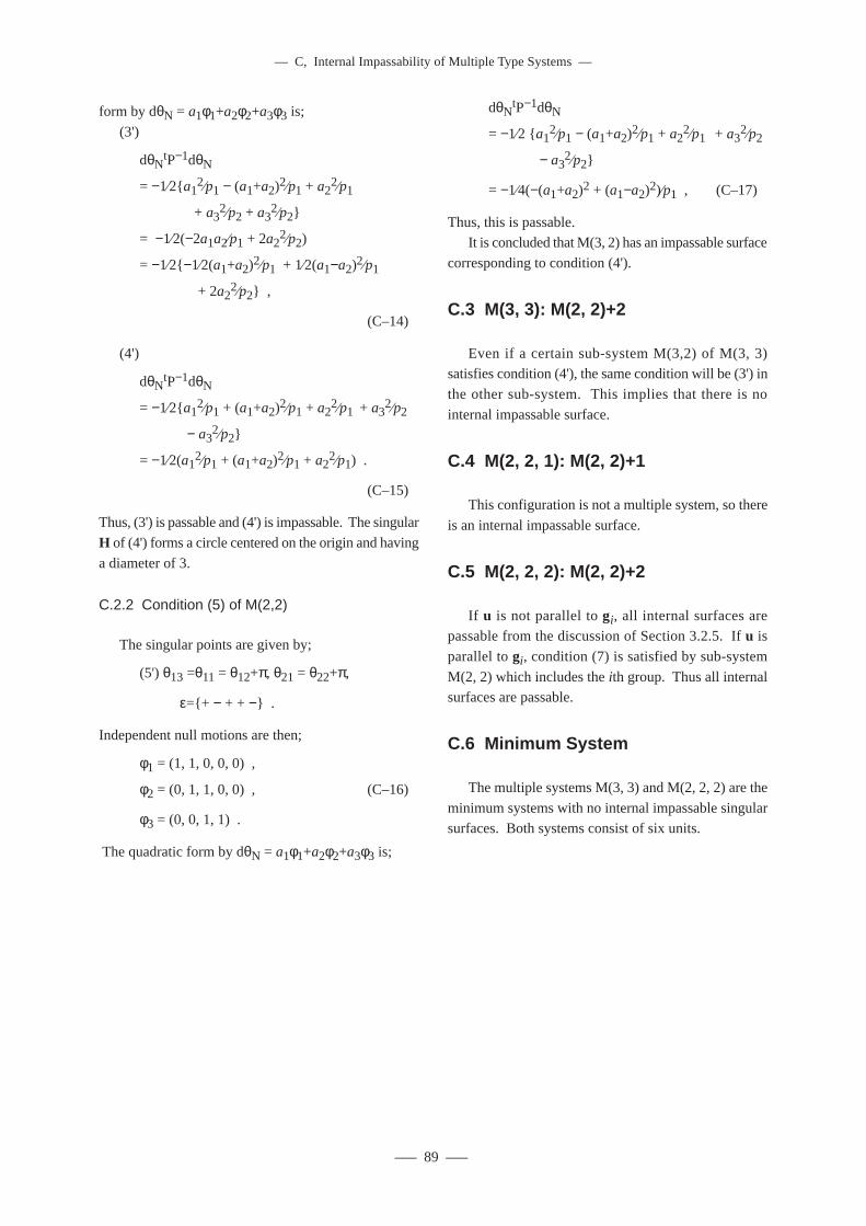
––– 89 –––
form by dθN = a1φ1+a2φ2+a3φ3 is;
(3')
dθNtP−1dθN
= −1⁄2{a12⁄p1 − (a1+a2)2⁄p1 + a2
2⁄p1
+ a32⁄p2 + a3
2⁄p2}
= −1⁄2(−2a1a2⁄p1 + 2a22⁄p2)
= −1⁄2{−1⁄2(a1+a2)2⁄p1 + 1⁄2(a1−a2)2⁄p1
+ 2a22⁄p2} ,
(C–14)
(4')
dθNtP−1dθN
= −1⁄2{a12⁄p1 + (a1+a2)2⁄p1 + a2
2⁄p1 + a32⁄p2
− a32⁄p2}
= −1⁄2(a12⁄p1 + (a1+a2)2⁄p1 + a2
2⁄p1) .
(C–15)
Thus, (3') is passable and (4') is impassable. The singular
H of (4') forms a circle centered on the origin and having
a diameter of 3.
C.2.2 Condition (5) of M(2,2)
The singular points are given by;
(5') θ13 =θ11 = θ12+π, θ21 = θ22+π,
ε={+ − + + −} .
Independent null motions are then;
φ1 = (1, 1, 0, 0, 0) ,
φ2 = (0, 1, 1, 0, 0) , (C–16)
φ3 = (0, 0, 1, 1) .
The quadratic form by dθN = a1φ1+a2φ2+a3φ3 is;
dθNtP−1dθN
= −1⁄2 {a12⁄p1 − (a1+a2)2⁄p1 + a2
2⁄p1 + a32⁄p2
− a32⁄p2}
= −1⁄4(−(a1+a2)2 + (a1−a2)2)⁄p1 , (C–17)
Thus, this is passable.It is concluded that M(3, 2) has an impassable surface
corresponding to condition (4').
C.3 M(3, 3): M(2, 2)+2
Even if a certain sub-system M(3,2) of M(3, 3)satisfies condition (4'), the same condition will be (3') in
the other sub-system. This implies that there is no
internal impassable surface.
C.4 M(2, 2, 1): M(2, 2)+1
This configuration is not a multiple system, so there
is an internal impassable surface.
C.5 M(2, 2, 2): M(2, 2)+2
If u is not parallel to gi, all internal surfaces arepassable from the discussion of Section 3.2.5. If u is
parallel to gi, condition (7) is satisfied by sub-system
M(2, 2) which includes the ith group. Thus all internalsurfaces are passable.
C.6 Minimum System
The multiple systems M(3, 3) and M(2, 2, 2) are the
minimum systems with no internal impassable singularsurfaces. Both systems consist of six units.
–– C, Internal Impassability of Multiple Type Systems ––

–– Technical Report of Mechanical Engineering Laboratory No.175 ––
––– 90 –––
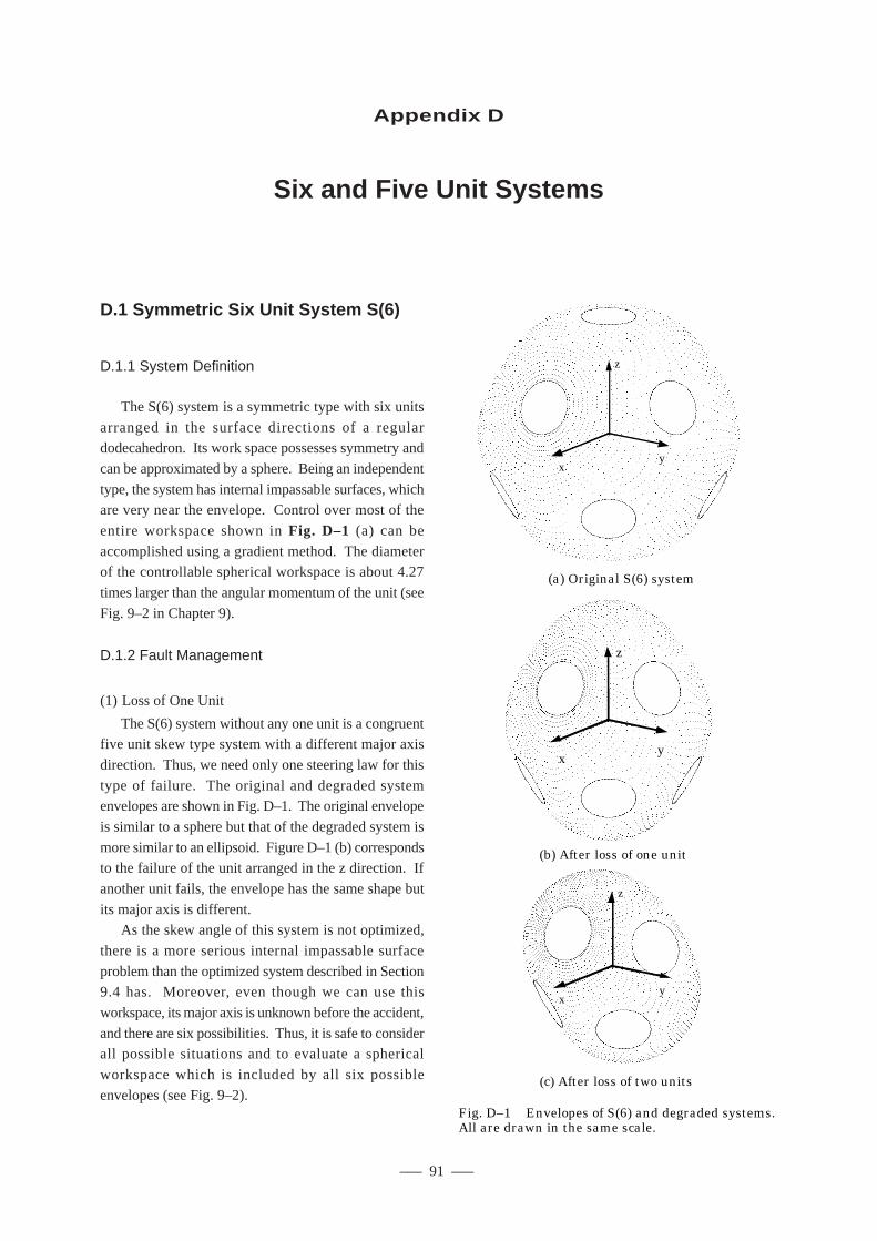
––– 91 –––
Appendix D
Six and Five Unit Systems
D.1 Symmetric Six Unit System S(6)
D.1.1 System Definition
The S(6) system is a symmetric type with six units
arranged in the surface directions of a regulardodecahedron. Its work space possesses symmetry and
can be approximated by a sphere. Being an independent
type, the system has internal impassable surfaces, whichare very near the envelope. Control over most of the
entire workspace shown in Fig. D–1 (a) can be
accomplished using a gradient method. The diameterof the controllable spherical workspace is about 4.27
times larger than the angular momentum of the unit (see
Fig. 9–2 in Chapter 9).
D.1.2 Fault Management
(1) Loss of One Unit
The S(6) system without any one unit is a congruentfive unit skew type system with a different major axis
direction. Thus, we need only one steering law for this
type of failure. The original and degraded systemenvelopes are shown in Fig. D–1. The original envelope
is similar to a sphere but that of the degraded system is
more similar to an ellipsoid. Figure D–1 (b) correspondsto the failure of the unit arranged in the z direction. If
another unit fails, the envelope has the same shape but
its major axis is different.As the skew angle of this system is not optimized,
there is a more serious internal impassable surface
problem than the optimized system described in Section9.4 has. Moreover, even though we can use this
workspace, its major axis is unknown before the accident,
and there are six possibilities. Thus, it is safe to considerall possible situations and to evaluate a spherical
workspace which is included by all six possible
envelopes (see Fig. 9–2).
(b) After loss of one unit
z
yx
(a) Original S(6) system
z
yx
(c) After loss of two units
z
yx
Fig. D–1 Envelopes of S(6) and degraded systems.All are drawn in the same scale.
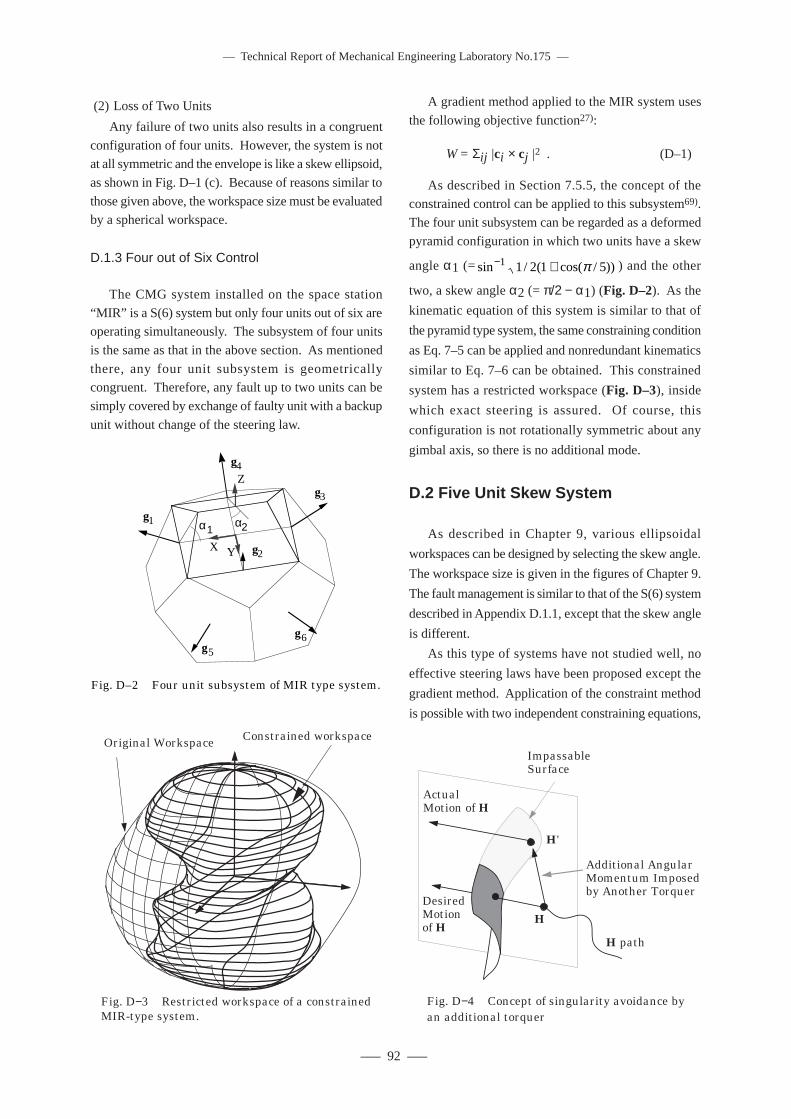
–– Technical Report of Mechanical Engineering Laboratory No.175 ––
––– 92 –––
(2) Loss of Two Units
Any failure of two units also results in a congruent
configuration of four units. However, the system is notat all symmetric and the envelope is like a skew ellipsoid,
as shown in Fig. D–1 (c). Because of reasons similar to
those given above, the workspace size must be evaluatedby a spherical workspace.
D.1.3 Four out of Six Control
The CMG system installed on the space station
“MIR” is a S(6) system but only four units out of six areoperating simultaneously. The subsystem of four units
is the same as that in the above section. As mentioned
there, any four unit subsystem is geometricallycongruent. Therefore, any fault up to two units can be
simply covered by exchange of faulty unit with a backup
unit without change of the steering law.
A gradient method applied to the MIR system uses
the following objective function27):
W = Σij |ci × cj |2 . (D–1)
As described in Section 7.5.5, the concept of theconstrained control can be applied to this subsystem69).
The four unit subsystem can be regarded as a deformed
pyramid configuration in which two units have a skew
angle α1 (= sin / ( cos( / ))− +1 1 2 1 5π ) and the other
two, a skew angle α2 (= π/2 − α1) (Fig. D–2). As the
kinematic equation of this system is similar to that of
the pyramid type system, the same constraining condition
as Eq. 7–5 can be applied and nonredundant kinematics
similar to Eq. 7–6 can be obtained. This constrained
system has a restricted workspace (Fig. D–3), inside
which exact steering is assured. Of course, this
configuration is not rotationally symmetric about any
gimbal axis, so there is no additional mode.
D.2 Five Unit Skew System
As described in Chapter 9, various ellipsoidal
workspaces can be designed by selecting the skew angle.
The workspace size is given in the figures of Chapter 9.
The fault management is similar to that of the S(6) system
described in Appendix D.1.1, except that the skew angle
is different.
As this type of systems have not studied well, no
effective steering laws have been proposed except the
gradient method. Application of the constraint method
is possible with two independent constraining equations,
α1 α2g1
g2
g3
g4
g5
g6
X Y
Z
Fig. D–2 Four unit subsystem of MIR type system.
Fig. D−4 Concept of singularity avoidance by an additional torquer
H
H'
Desired Motion of H
Additional Angular Momentum Imposed by Another Torquer
Actual Motion of H
H path
Impassable Surface
Original Workspace Constrained workspace
Fig. D−3 Restricted workspace of a constrained MIR-type system.
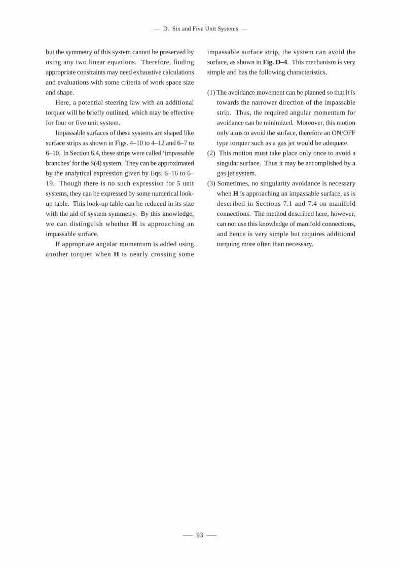
––– 93 –––
but the symmetry of this system cannot be preserved by
using any two linear equations. Therefore, finding
appropriate constraints may need exhaustive calculations
and evaluations with some criteria of work space size
and shape.
Here, a potential steering law with an additional
torquer will be briefly outlined, which may be effective
for four or five unit system.
Impassable surfaces of these systems are shaped like
surface strips as shown in Figs. 4–10 to 4–12 and 6–7 to
6–10. In Section 6.4, these strips were called ‘impassable
branches’ for the S(4) system. They can be approximated
by the analytical expression given by Eqs. 6–16 to 6–
19. Though there is no such expression for 5 unit
systems, they can be expressed by some numerical look-
up table. This look-up table can be reduced in its size
with the aid of system symmetry. By this knowledge,
we can distinguish whether H is approaching an
impassable surface.
If appropriate angular momentum is added using
another torquer when H is nearly crossing some
impassable surface strip, the system can avoid the
surface, as shown in Fig. D–4. This mechanism is very
simple and has the following characteristics.
(1) The avoidance movement can be planned so that it is
towards the narrower direction of the impassable
strip. Thus, the required angular momentum for
avoidance can be minimized. Moreover, this motion
only aims to avoid the surface, therefore an ON/OFF
type torquer such as a gas jet would be adequate.
(2) This motion must take place only once to avoid a
singular surface. Thus it may be accomplished by a
gas jet system.
(3) Sometimes, no singularity avoidance is necessary
when H is approaching an impassable surface, as is
described in Sections 7.1 and 7.4 on manifold
connections. The method described here, however,
can not use this knowledge of manifold connections,
and hence is very simple but requires additional
torquing more often than necessary.
–– D. Six and Five Unit Systems ––

–– Technical Report of Mechanical Engineering Laboratory No.175 ––
––– 94 –––
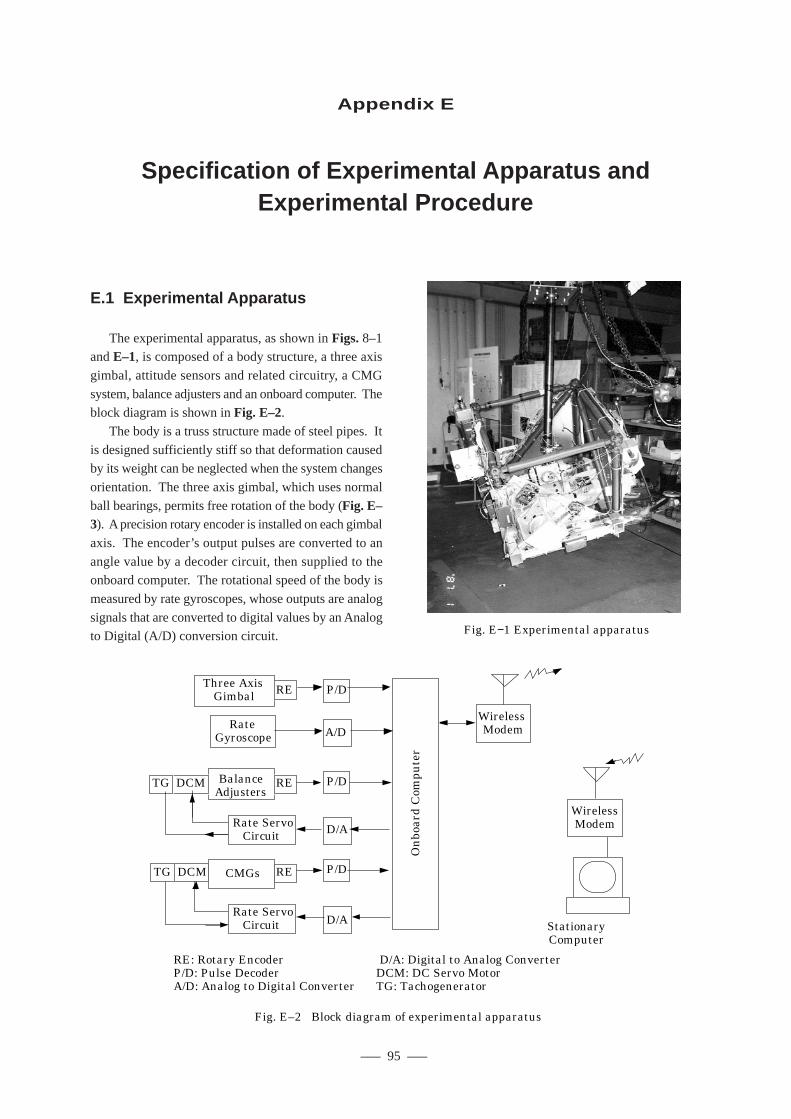
––– 95 –––
E.1 Experimental Apparatus
The experimental apparatus, as shown in Figs. 8–1and E–1, is composed of a body structure, a three axis
gimbal, attitude sensors and related circuitry, a CMG
system, balance adjusters and an onboard computer. Theblock diagram is shown in Fig. E–2.
The body is a truss structure made of steel pipes. It
is designed sufficiently stiff so that deformation causedby its weight can be neglected when the system changes
orientation. The three axis gimbal, which uses normal
ball bearings, permits free rotation of the body (Fig. E–3). A precision rotary encoder is installed on each gimbal
axis. The encoder’s output pulses are converted to an
angle value by a decoder circuit, then supplied to theonboard computer. The rotational speed of the body is
measured by rate gyroscopes, whose outputs are analog
signals that are converted to digital values by an Analogto Digital (A/D) conversion circuit.
Appendix E
Specification of Experimental Apparatus andExperimental Procedure
Fig. E−1 Experimental apparatus
Stationary Computer
RE: Rotary Encoder D/A: Digital to Analog ConverterP/D: Pulse Decoder DCM: DC Servo MotorA/D: Analog to Digital Converter TG: Tachogenerator
Fig. E–2 Block diagram of experimental apparatus
Three Axis Gimbal
Balance Adjusters
On
boar
d C
ompu
ter
P/D
P/D
P/D
D/A
D/A
Rate Gyroscope A/D
Wireless Modem
RE
REDCMTG
REDCMTG
Wireless Modem
Rate Servo Circuit
Rate Servo Circuit
CMGs
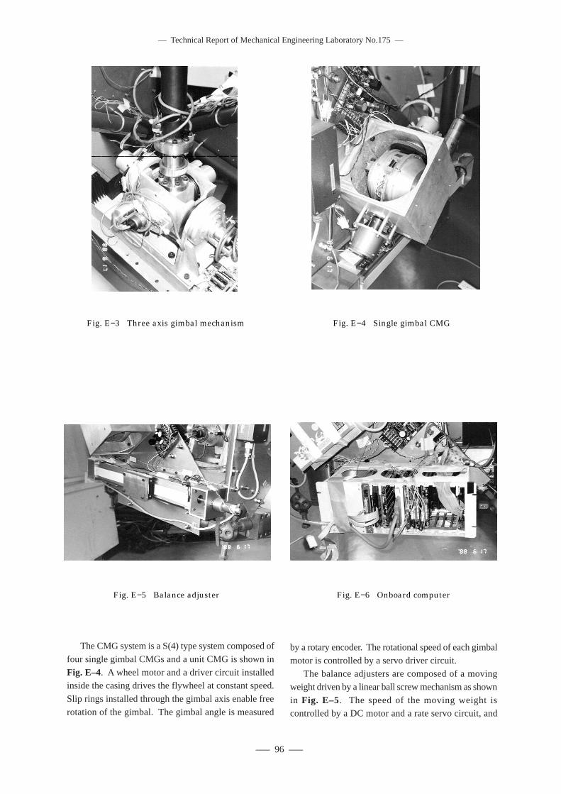
–– Technical Report of Mechanical Engineering Laboratory No.175 ––
––– 96 –––
The CMG system is a S(4) type system composed of
four single gimbal CMGs and a unit CMG is shown in
Fig. E–4. A wheel motor and a driver circuit installedinside the casing drives the flywheel at constant speed.
Slip rings installed through the gimbal axis enable free
rotation of the gimbal. The gimbal angle is measured
by a rotary encoder. The rotational speed of each gimbal
motor is controlled by a servo driver circuit.The balance adjusters are composed of a moving
weight driven by a linear ball screw mechanism as shown
in Fig. E–5. The speed of the moving weight iscontrolled by a DC motor and a rate servo circuit, and
Fig. E−3 Three axis gimbal mechanism Fig. E−4 Single gimbal CMG
Fig. E−5 Balance adjuster Fig. E−6 Onboard computer
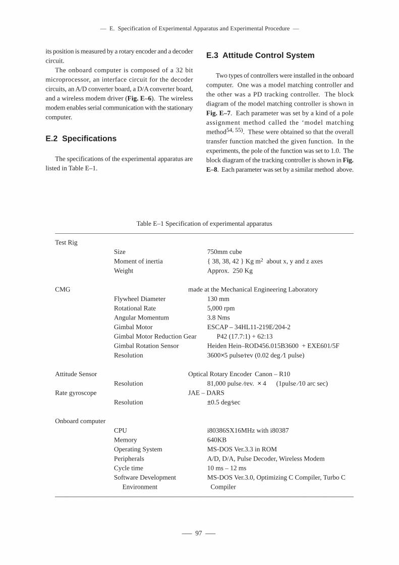
––– 97 –––
Table E–1 Specification of experimental apparatus
–––––––––––––––––––––––––––––––––––––––––––––––––––––––––––––––––––––––––––––––––––––––––
Test RigSize 750mm cube
Moment of inertia { 38, 38, 42 } Kg m2 about x, y and z axes
Weight Approx. 250 Kg
CMG made at the Mechanical Engineering Laboratory
Flywheel Diameter 130 mmRotational Rate 5,000 rpm
Angular Momentum 3.8 Nms
Gimbal Motor ESCAP – 34HL11-219E/204-2Gimbal Motor Reduction Gear P42 (17.7:1) + 62:13
Gimbal Rotation Sensor Heiden Hein–ROD456.015B3600 + EXE601/5F
Resolution 3600×5 pulse⁄rev (0.02 deg ⁄1 pulse)
Attitude Sensor Optical Rotary Encoder Canon – R10
Resolution 81,000 pulse ⁄rev. × 4 (1pulse ⁄10 arc sec)Rate gyroscope JAE – DARS
Resolution ±0.5 deg⁄sec
Onboard computer
CPU i80386SX16MHz with i80387
Memory 640KBOperating System MS-DOS Ver.3.3 in ROM
Peripherals A/D, D/A, Pulse Decoder, Wireless Modem
Cycle time 10 ms – 12 msSoftware Development MS-DOS Ver.3.0, Optimizing C Compiler, Turbo C
Environment Compiler
–––––––––––––––––––––––––––––––––––––––––––––––––––––––––––––––––––––––––––––––––––––––––
its position is measured by a rotary encoder and a decoder
circuit.
The onboard computer is composed of a 32 bitmicroprocessor, an interface circuit for the decoder
circuits, an A/D converter board, a D/A converter board,
and a wireless modem driver (Fig. E–6). The wirelessmodem enables serial communication with the stationary
computer.
E.2 Specifications
The specifications of the experimental apparatus arelisted in Table E–1.
E.3 Attitude Control System
Two types of controllers were installed in the onboard
computer. One was a model matching controller and
the other was a PD tracking controller. The blockdiagram of the model matching controller is shown in
Fig. E–7. Each parameter was set by a kind of a pole
assignment method called the ‘model matchingmethod54, 55). These were obtained so that the overall
transfer function matched the given function. In the
experiments, the pole of the function was set to 1.0. Theblock diagram of the tracking controller is shown in Fig.E–8. Each parameter was set by a similar method above.
–– E. Specification of Experimental Apparatus and Experimental Procedure ––
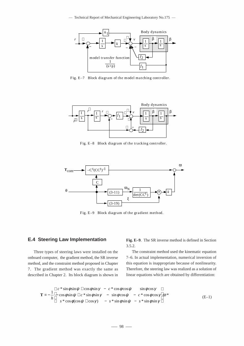
–– Technical Report of Mechanical Engineering Laboratory No.175 ––
––– 98 –––
E.4 Steering Law Implementation
Three types of steering laws were installed on the
onboard computer, the gradient method, the SR inverse
method, and the constraint method proposed in Chapter7. The gradient method was exactly the same as
described in Chapter 2. Its block diagram is shown in
T = −+ −
− + − −+ − −
1
h
c c
c c
s s s
* sin sin cos sin * cos cos sin cos
cos sin * sin sin sin cos * cos cos
* cos (cos cos ) * sin sin * sin sin
*
φ ψ φ γ φ ψ φ γφ ψ φ γ φ ψ φ γ
φ ψ γ φ ψ φ γω (E–1)
Fig. E–9. The SR inverse method is defined in Section3.5.2.
The constraint method used the kinematic equation
7–6. In actual implementation, numerical inversion ofthis equation is inappropriate because of nonlinearity.
Therefore, the steering law was realized as a solution of
linear equations which are obtained by differentiation:
Fig. E–7 Block diagram of the model matching controller.
s1
s1
f2
v ββ.
s1r +
+
−
f1
−k
k1
−
+
(s+p)1
model transfer function
Body dynamics
Fig. E–8 Block diagram of the tracking controller.
s1
s1
f2
v βf1
β.
r⋅⋅s1
s1
r⋅ r +
−
++
+
+ −
Body dynamics
Fig. E–9 Block diagram of the gradient method.
–Ct(CCt)-1Tcom
θωN
(3-11)
(3-19)ξ
det(CCt)1
+ω
k×
C
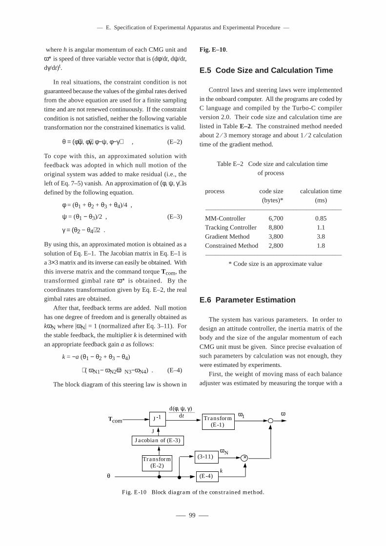
––– 99 –––
where h is angular momentum of each CMG unit and
ω∗ is speed of three variable vector that is (dφ/dt, dψ/dt,
dγ/dt)t.
In real situations, the constraint condition is not
guaranteed because the values of the gimbal rates derivedfrom the above equation are used for a finite sampling
time and are not renewed continuously. If the constraint
condition is not satisfied, neither the following variabletransformation nor the constrained kinematics is valid.
θ = (φ+ψ, φ+γ, φ−ψ, φ−γ) , (E–2)
To cope with this, an approximated solution with
feedback was adopted in which null motion of theoriginal system was added to make residual (i.e., the
left of Eq. 7–5) vanish. An approximation of (φ, ψ, γ) isdefined by the following equation.
φ = (θ1 + θ2 + θ3 + θ4)/4 ,
ψ = (θ1 − θ3)/2 , (E–3)
γ = (θ2 − θ4)/2 .
By using this, an approximated motion is obtained as a
solution of Eq. E–1. The Jacobian matrix in Eq. E–1 is
a 3×3 matrix and its inverse can easily be obtained. Withthis inverse matrix and the command torque Tcom, the
transformed gimbal rate ω∗ is obtained. By the
coordinates transformation given by Eq. E–2, the realgimbal rates are obtained.
After that, feedback terms are added. Null motion
has one degree of freedom and is generally obtained askωN where |ωN| = 1 (normalized after Eq. 3–11). For
the stable feedback, the multiplier k is determined with
an appropriate feedback gain a as follows:
k = −a (θ1 − θ2 + θ3 − θ4)
⋅ ( ωN1− ωN2+ωN3−ωN4) . (E–4)
The block diagram of this steering law is shown in
Fig. E–10.
E.5 Code Size and Calculation Time
Control laws and steering laws were implemented
in the onboard computer. All the programs are coded byC language and compiled by the Turbo-C compiler
version 2.0. Their code size and calculation time are
listed in Table E–2. The constrained method neededabout 2 ⁄ 3 memory storage and about 1 ⁄ 2 calculation
time of the gradient method.
Table E–2 Code size and calculation timeof process
process code size calculation time (bytes)* (ms)
––––––––––––––––––––––––––––––––––––––––––
MM-Controller 6,700 0.85Tracking Controller 8,800 1.1
Gradient Method 3,800 3.8
Constrained Method 2,800 1.8––––––––––––––––––––––––––––––––––––––––––
* Code size is an approximate value
E.6 Parameter Estimation
The system has various parameters. In order todesign an attitude controller, the inertia matrix of the
body and the size of the angular momentum of each
CMG unit must be given. Since precise evaluation ofsuch parameters by calculation was not enough, they
were estimated by experiments.
First, the weight of moving mass of each balanceadjuster was estimated by measuring the torque with a
Fig. E-10 Block diagram of the constrained method.
J-1Tcom
θ
ωN
(E-4)
+ω
×Transform(E-2)
Jacobian of (E-3)
J
d(φ, ψ, γ)dt ω1
k
(3-11)
Transform(E-1)
–– E. Specification of Experimental Apparatus and Experimental Procedure ––

–– Technical Report of Mechanical Engineering Laboratory No.175 ––
––– 100 –––
scale when the position of the mass was moved in a step-
by-step manner. Then a certain fixed torque was applied
by this mechanism while the body was stabilized by theCMG system. The total angular momentum of the CMG
system linearly increased by the constant disturbance
torque. From the kinematic relation and measuredgimbal angles, the size of angular momentum of each
unit was thereby estimated.
Then, the body was rotated by the CMG system,
generating a constant torque on the principal axis of the
body. It was presumed that the principal axes (eigenaxesof the inertia matrix) were the same as the structure’s
frame directions. Trials about three axes were then made.
By comparing the measured angular velocity of the bodywith the CMG angular momentum, the moment of inertia
about each axis was estimated. The estimated values
are included in the specification of Table E–1.
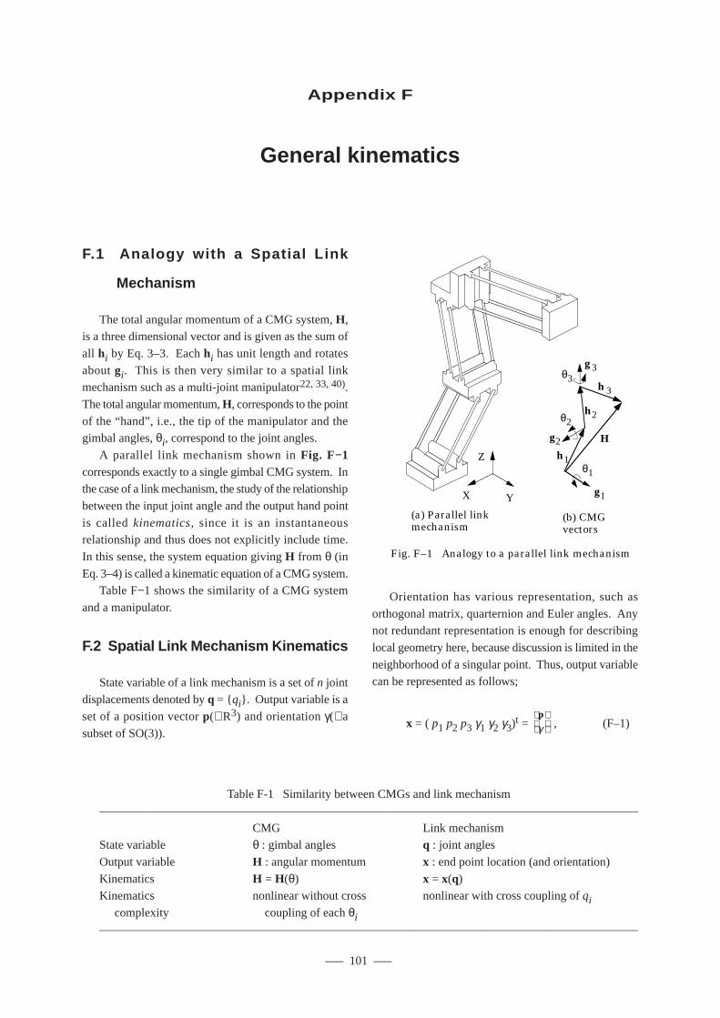
––– 101 –––
F.1 Analogy with a Spatial Link
Mechanism
The total angular momentum of a CMG system, H,is a three dimensional vector and is given as the sum of
all hi by Eq. 3–3. Each hi has unit length and rotates
about gi. This is then very similar to a spatial linkmechanism such as a multi-joint manipulator22, 33, 40).
The total angular momentum, H, corresponds to the point
of the “hand”, i.e., the tip of the manipulator and thegimbal angles, θi, correspond to the joint angles.
A parallel link mechanism shown in Fig. F−1corresponds exactly to a single gimbal CMG system. Inthe case of a link mechanism, the study of the relationship
between the input joint angle and the output hand point
is called kinematics, since it is an instantaneousrelationship and thus does not explicitly include time.
In this sense, the system equation giving H from θ (in
Eq. 3–4) is called a kinematic equation of a CMG system.Table F−1 shows the similarity of a CMG system
and a manipulator.
F.2 Spatial Link Mechanism Kinematics
State variable of a link mechanism is a set of n jointdisplacements denoted by q = {qi}. Output variable is a
set of a position vector p(∈R3) and orientation γ(∈a
subset of SO(3)).
Orientation has various representation, such as
orthogonal matrix, quarternion and Euler angles. Anynot redundant representation is enough for describing
local geometry here, because discussion is limited in the
neighborhood of a singular point. Thus, output variablecan be represented as follows;
x = ( p1 p2 p3 γ1 γ2 γ3)t =
pγ
, (F–1)
Appendix F
General kinematics
Table F-1 Similarity between CMGs and link mechanism
–––––––––––––––––––––––––––––––––––––––––––––––––––––––––––––––––––––––––––––––––––––––––
CMG Link mechanismState variable θ : gimbal angles q : joint angles
Output variable H : angular momentum x : end point location (and orientation)
Kinematics H = H(θ) x = x(q)Kinematics nonlinear without cross nonlinear with cross coupling of qi complexity coupling of each θi–––––––––––––––––––––––––––––––––––––––––––––––––––––––––––––––––––––––––––––––––––––––––
X Y
Z
g1
g2
g3
h1
h2
h3
H
θ1
θ2
θ3
Fig. F–1 Analogy to a parallel link mechanism
(a) Parallel link mechanism
(b) CMG vectors
–– Technical Report of Mechanical Engineering Laboratory No.175 ––
––– 102 –––
Kinematic equation is a nonlinear equation from joint
displacements q to the output x. Exact expression of
this equation is found in most literature.
x = f(q) . (F–2)
Differentiation of the equation leads to,
dx = dq = J dq . (F–3)
Usual definition of Jacobian with axial velocity of
the end-effector ω is given as follows,
dp / dt
ω
= J*dq / dt . (F–4)
From assumption above, there is a non-singular
transformation between ω and dγ/dt as,
ω = Γ dγ/dt . (F–5)
Therefore,
∂f / ∂q = J = Γ∗ -1 J∗ , where Γ∗ = I
G3 0
0
.
(F–6)
Keeping generality, we can take the origin where the
transformation Γ∗ is identity hence J = J∗.
F.3 Singularity
Singular state is a case where the matrix J does not
have full rank. This means that,
det ( J ) = 0 , (F–7)
and there exists at least one direction, denoted as ζ, inthe tangent space of the x space, which satisfies,
ζt J = 0 , where | ζ | = 1 . (F–8)
This direction can be called a singular direction. The
difference between CMGs and a manipulator is that thereis no explicit expression which gives singular state
variable q from this singular direction ζ as in Eqs. 4–2
and 4–3.
F.4 Passability
In order to classify singularity, small displacement
from the singular point is expressed as a Taylor series,
x(q+dq) − x(q)
= Σi ∂f/∂qi dqi + 1/2 Σij ∂f2/∂qi∂qj
dqi dqj
+ O(dq3) . (F–9)
Then, component of the singular direction is extractedand the 3rd and higher order terms are omitted.
As taking scalar product with ζ, first term vanishes,
∆x = ζt { x(q+dq) − x(q) }
= 1/2 Σij (ζ ⋅ ∂f2/∂qi∂qj ) dqi dqj
= 1/2 dqt Q dq . (F–10)
where matrix Q is,
Q = ( ζt ∂f2/∂qi∂qj ) . (F–11)
This matrix is not so simple as a diagonal matrix Pin the case of CMGs. Moreover, signature is not
explicitly obtained from this matrix Q.
The next step is to decompose this quadratic forminto two sub-quadratic forms. One rises from the curved
hyper surface of singular state and the other from the
displacement from this hyper surface. This is obtainedby decomposing dq into two parts, dqS which keeps
singularity and homogeneous motion dqN:
dq = dqN + dqS . (F–12)
The definition of dqN and dqS is,
det ( J( q+dqS) )=0 ,
J dqN = 0 . (F–13)
If a singular state is characterized by one direction
ζ, the dimension of the singular hyper surface is 5 and
so is the vector space of dqS. In this case the rank of J is5. The kernel of J, that is a vector space of dqN, is n-5
dimensional.
Substituting (F–12) into (F–10) leads to,
∆x = 1/2d(qS)tQdqS + 1/2 (dqN)tQdqN
+ (dqS)tQdqN . (F–14)
The third term in the right will be shown zero. In order
to prevent complication, let partial derivatives of thefunction f = (fi) be denoted by index with comma, such
as,
fi,j = ∂fi / ∂qj . (F–15)
Singular direction is defined again as,
––– 103 –––
Σi ζi fi,j = 0 , (F–16)
and its differential is
Σi dζi fi,j + Σi ζi Σj fi,jk dqSk = 0 . (F–17)
Then,
(dqN)t Q dqS
= 1/2 Σi ζi ΣjΣk fi,jk dqNj dqS
k
= 1/2 Σj{ Σi ζi Σk fi,jk dqSk }dqN
j
= − 1/2 ΣjΣi dζi fi,j dqNj
= − 1/2 Σi dζi { Σj fi,j dqNj}
= − 1/2 dζt (J dqN)
= 0 . (F–18)
Thus the quadratic form ∆x is divided into two as,
∆x = 1/2(dqS)tQdqS + 1/2 (dqN)tQdqN
= 1/2 Σijk fi,jk ζi dqSj dqS
k
+ 1/2 Σijk fi,jk ζi dqNj dqN
k . (F–19)
The first term is a kind of curvature of the singular
hyper surface. The second quadratic form gives
passability. There is a restriction for the above
discussion, i.e., the expression (F–12) is not alwayspossible. It is neither possible nor the last equation be
assured, when the product space of two linear spaces
spanned by {dqS} and {dqN} do not cover whole tangentspace.
A similar expression of passability is thus obtained
generally as CMGs but the following differences andproblems are remaining for further study;
(1) No expression of Gaussian curvature is obtained(2) Neither simple description of whole quadratic form
nor whole signature is obtained. This is because there is
no general solution of singular state from the direction ζand sign {εi}.
(3) Dimension of the singular hyper surface (= 5) is
greater than that of remaining space ( =n − 5), in usualcase, because the number of the joints is not greater than
10. Therefore it seems easier to deal with the quadratic
form directly.
–– F. General Kinematics ––

–– Technical Report of Mechanical Engineering Laboratory No.175 ––
––– 104 –––
––– 105 –––
1) The Bendix Corp.: Control Moment Gyroscope
Gimbal Actuator Study, AFFDL-TR-66-158,
210p, 1966.
2) Cramer, P.S., Josephson, J.T.: CMG Assembly
Life Test and Engineering Evaluation Test M-509
Experiment, NASA-CR-115280, 35p, 1970.
3) Fikes, E.H.: Control Moment Gyro for Skylab,
NASA-TM-X-64586, 22p, 1971.
4) Auclair, G.F., Wells, R.C.: Control Moment Gyro
Selection and Design Criteria, AIAA Guidance,
Control and Flight Mechanics Conference AIAA
Paper No.70-976, 10p, 1970.
5) Liska, D.J.: A Two-degree-of-freedom Control
Moment Gyro for High-Accuracy Attitude
Control, J. Spacecraft, 75-83, 1968.
6) Chubb, W.b., Schultz, D.N., Seltzer, S.M.:
Attitude Control and Precision Pointing of the
Apollo Telescope Mount, AIAA Guidance,
Control and Flight Dynamics Conference, AIAA
No.67-534, 1967.
7) O’connor, B.J., Morine, L.A.: A Description and
the CMG and its Application to Space Vehicle
Control, AIAA Guidance, Control and Flight
Dynamics Conference, AIAA No.67-589, 1967.
8) Morine, L.A., O’Conner, B.J.: The Description
of the CMG and its Application to Space Vehicle
Control, Bendix Corp. Publication No. 674-7,
37p, 1967.
9) Bendix Corp.: ATM CMG/EPEA, NASA-CR-
120760, 188p, 1975.
10) Kyle, R.G.: Optimal Feedback control for
Nonlinear Control Moment Gyro Systems,
NASA-TM-X-67790 (Ph, D. Thesis - Verginia
Univ. ), 119 p., 1969.
11) Coon, T.R., Irby, J.E.: Skylab Attitude Control
System, IBM Journal of Research Development,
pp. 58-66, 1976.
12) The Corporation: Study to Definite Logic
Associated with CMGs to Maneuver and Stabilize
an Orbiting Spacecraft - Final Report, NASA-CR-
134207, 511p, 1973.
13) Winder, S.W.: Steering Laws for Double-Gimbal
Control-Moment Gyros, NASA-CP007, 157-173,
1978.
14) NASA MSFC: A Comparison of CMG Steering
Laws for High Energy Astronomy Observatories(
HEAOs), NASA TM X-64727, p.127, 1972.
15) Crenshaw, J.W.: 2-Speed, a Single Gimbal CMG
Attitude Control System, TR-243-1139(NASA
CR) Northrop Services Inc., 38p, 1972.
16) Yoshikawa, T.: Steering Law for Roof Type
Configuration Control Moment Gyro System,
Automatica, 13, pp.359-368, 1979.
17) Elrod, B.D., Anderson, G.M.: Equilibrium
Properties of the Skylab CMG Rotation Law -
Case 620, NASA-CR-126140 (Bellcomm TM-
72-1022-2), p.79, 1972.
18) Kennel, H.F.: Steering Law for Parallel Mounted
Double-Gimbaled Control Moment Gyros,
NASA-TM-X-64930, 34p, 1975.
19) Colburn, B.K. and White, L.R.: Computational
Considerations for a Spacecraft Attitude Control
System Employing Control Moment Gyro,
Journal of Spacecraft, Vol. 14, No. 1, 40-53, 1977.
20) H.F.Kennel: Steering Law for Parallel Mounted
Double-Gimbaled Control Moment Gyros –
Revision A, NASA-TM-82390, 22p, 1981.
21) Yoshikawa, T.: A Steering Law for Three Double
Gimbal Control Moment Gyro System, NASA-
TM-X-64926, 1975.
22) Margulies, G. and Aubrun, J.N.: Geometric
Theory of Single-Gimbal Control Moment Gyro
System, Journal of Astronautical Sciences, Vol.
26, No.2, pp. 159-191, 1978.
23) Tokar, E.N.: Problems of Gyroscopic Stabilizer
Control, Cosmic Research, pp.141-147, 1978
(original: Kosmicheskie Issledovaniya Vol.16,
No.2, pp.179-187, 1978).
24) Tokar, E.N.: Efficient Design of Powered
Gyrostabilizer Systems, Cosmic Research, pp.16-
References
–– Technical Report of Mechanical Engineering Laboratory No.175 ––
––– 106 –––
23, 1978. (original: Kosmicheskie Issledovaniya
Vol.16, No.1, pp.22-30, 1978)
25) Tokar, E.N.: Effect of Limiting Supports on Gyro
Stabilizer, Cosmic Research, pp.413-420, 1979.
(original: Kosmicheskie Issledovaniya Vol.16,
No.4, pp.505-513, 1978)
26) Tokar, E.N. and Platonov, V.N. : Singular Surfaces
in Unsupported Gyrodyne Systems, Cosmic
Research, pp.547-555, 1979 (or iginal :
Kosmicheskie Issledovaniya Vol.16, No.5,
pp.675-685, 1978).
27) Branets, V.N. et al.: Development Experience of
the Attitude Control System Using Single-Axis
Control Moment Gyros for Long-Term Orbiting
Space Stations, 38th Congress of the International
Astronoutical Federation, IAF-87-04, 8p, 1987.
28) Kurokawa, H., Yajima, N., Usui, S.: A New
Steering Law of a Single gimbal CMG System
of Pyramid Configuration, Proceedings of IFAC
Automatic Control in Space, pp.251-257, 1985.
29) Kurokawa, H., Yajima, N.: A Study of Single
Gimbal CMG System, Proceedings of 15th
International Symposium on Space Technology
and Science (ISTS), pp.1219-1224, 1986.
30) Kurokawa, H., Yajima, N.: On the singularity of
a single gimbal CMG, Journal of the Japan
Society for Aeronautical and Space Sciences, Vol.
34, No. 395, pp.29-34, 1986. (in Japanese).
31) Kurokawa, H., Yajima, N.: A Study on Control
Moment Gyro Systems - Singularity and Steering
Laws of Single Gimbal CMG systems, Report of
Mechanical Engineering Laboratory, No. 140,
1987, (in Japanese).
32) Kurokawa, H: A Study of CMG Systems - for
Selection and Evaluation, Proceedings of 16th
International Symposium on Space Technology
and Science (ISTS), pp.1243-1249, 1988
33) Kurokawa, H.: Attitude Control by using Control
Moment Gyros, Systems, Control and
Information, Vol. 33, No. 4, pp.157-164, 1989,
(in Japanese).
34) D.E.Cornick: Singularity Avoidance Control
Laws for Single Gimbal Control Moment Gyros,
Proceedings of AIAA Guidance and Control
Conference 79-1698, pp.20-33, 1979. (Martin
Marietta Corp.
35) Hefner, R.D. and McKenzie, C.H.: A technique
for maximizing the torque capability of control
moment gyro systems, Astrodynamics Vol.54
(Proceedings of AAS/AIAA Astrodynamics
Conference Vol.2), 905-920, 1983.
36) Kurokawa, H., Yajima, N., Usui, S.: A CMG
Attitude Control System for Balloon Use,
Proceedings of 14th International Symposium on
Space Technology and Science (ISTS), pp. 1211-
1216, 1984.
37) Bauer, S.R.: Difficulties Encountered In Steering
Single Gimbal CMG’s, Space Guidance and
Navigation Memo No.10E-87-09, The Charles
Stark Draper Laboratory, Inc.
38) Vadali, S.R., Oh, H.S., and Walker, S.R.: Preferred
Gimbal Angles for Single Gimbal Control
Moment Gyros, Journal of Guidance, Control, and
Dynamics, Vol.13, No.6, pp.1090–1095, 1990.
39) Kurokawa, H.: Exact Singularity Avoidance
Control of the Pyramid Type CMG System,
Proceedings of AIAA Guidance, Navigation, and
Control Conference, pp. 170-180, Aug., 1994.
40) Bedrossian, N.S.: Steering Law Design for
Redundant Single Gimbal Control Moment Gyro
Systems, NASA-CR-172008 (M.S.Thesis of
Massachusetts Institude of Technology, CSDL-
T-965), 138p, 1987.
41) Bedrossian, N.S., Paradiso, J., Bergmann, E.V.,
Rowell, D.: Steering Law Design for Redundant
Single-Gimbal Control Moment Gyroscope,
AIAA Journal of Guidance, Control, and
Dynamics, Vol. 13, No. 6, pp.1083-1089, 1990.
42) Paradiso, J.: Global Steering of Single Gimballed
Control Moment Gyroscopes Using a Directed
Search, AIAA Journal of Guidance, Control, and
Dynamics, Vol. 15, No.5, pp. 1236–1244, 1992.
43) Paradiso, J.: A Search-Based Approach to Steering
Single Gimbaled CMGs, CSDL-R-2261, 183p,
1991.
44) Vadali, S.R., Krishnan, S.: Suboptimal Command
Generation for Control Moment Gyroscopes and
Feedback Control of Spacecraft, Proceedings of
AIAA Guidance, Navigation and Control
Conference, pp. 637-646, Aug., 1994.
45) Seltzer, S.M.: CMG-Induced LST Dynamics,
NASA-TM-X-64833, 80p, 1974.
––– 107 –––
46) Seltzer, S.M.: Large Space Telescope Oscillation
Induce by CMG Friction, Journal of Spacecraft,
Vol. 12, No. 2, 96-105, 1975.
47) Seltzer, S.M., Kuo, B.C., Singh, G.: Limit Cycle
Analysis of Large Space Telescope with CMG
Nonlinearity, NASA-TM-X-64939, 20p, 1975.
48) Linden, S.P.: Precision CMG Control for High-
Accuracy Pointing, Proceedings of AIAA
Guidance and Control Conference, AIAA No. 73-
871, 7p.,1973.
49) Rybak, S.C. et al: Achieving Ultrahigh Accuracy
with a Body Pointing CMG/RW Control System,
Proceedings of AIAA Guidance and Control
Conference (AAS/AIAA Astrodynamics
Conference), 1973.
50) Paradiso, J.: A Highly Adaptable Steering/
Selection Procedure for Combined CMG/RCS
Spacecraft Control, CSDL-P-2653, 20p, 1986.
51) NASA Langley Research Center: Integrated
Power/Attitude Control System (IPACS), NASA-
CP-2290, 1983
52) Kalley Jr., J.J., Mork, H.L.: Development and Air
Bearing Test of a Double Gimbaled Momentum
Wheel Attitude Control System, Proceedings of
AIAA 5th Communications Satellite Systems
Conference AIAA Paper No. 74-488, 16p, 1974.
53) Yajima, N., Kurokawa, H, Kitahara, T: A
Simulation Platform for Three-Axis Attitude
Control of a Large Balloon Gondola, Proceedings
of 15th International Symposium on Space
Technology and Science (ISTS), pp.1555, 1560,
1986.
54) Suzuki, A., Kurokawa, H., Kokaji, S.: Three Axis
Control of an Experimental Platform using
CMGs, Proceedings of 18th International
Symposium on Space Technology and Science
(ISTS), pp.1059-1066, 1992.
55) Suzuki, A., Kurokawa, H., Kokaji, S: Robust
Attitude Control using a CMG System and an
Experiment with a Simulation Platform,
Proceedings of 12th IFAC Automatic Control in
Aerospace 1992, pp. 197-202, 1992.
56) Yoshikawa, T.: Manipulability of Robotic
Mechanisms, 2nd International Symposium on
Robotics Research, pp. 20-23, 1984.
57) Bedrossian, N.S.: Classification of Singular
Configurations for Redundant Manipulators,
Proceedings of IEEE International Conference on
Robotics and Automation, No.2, pp.818-823,
1990.
58) Bedrossian, N.S.: Characterizing Spatial
Redundant Manipulator Singular i t ies,
Proceedings of IEEE International Conference on
Robotics and Automation, No.1, pp.714-719,
1990.
59) Gott l ieb, D.H.: Robots and Topology,
Proceedings of IEEE International Conference on
Robotics and Automation, pp.1689-1691, 1986.
60) Burdick, J.W.: On the Inverse Kinematics of
Redundant Manipulators: Characterization of the
Self-Motion Manifolds, Proceedings of IEEE
International Conference on Robotics and
Automation, pp.264-270, 1989.
61) Pai, D.K., Leu, M.C.: Generic Singularities of
Robot Manipulators, Proceedings of IEEE
International Conference on Robotics and
Automation, pp.738-744, 1989.
62) Rodden, J.J.: Stabilization and Control of Space
Test Program 71-2, Proceedings of 7th IFAC
World Congress, Vol.7, No.2, ,pp.1213-1220,
1979.
63) Liu, T.C., Chubb, W.b., Seltzer, S.M., Thompson,
Z.: Optimal control of a variable spin speed CMG
system for space vehicles, Proceedings of IEEE
conference on Decision and Control, 722-726,
1973.
64) Bendix: Spacecraft CMG experience, The Bendix
Corporation, May, 1983.
65) Bedrossian, N.S., Paradiso, J., Bergmann, E.V.,
Rowell, D.: Redundant Single Gimbal Control
Moment Gyroscope Singularity Analysis, AIAA
Journal of Guidance and Control Dynamics, Vol.
13, No. 6, pp.1096-1101, 1990.
66) Kurokawa, H.: Geometrical View to Steering of
the Pyramid Type CMG System, Proceedings of
18th International Symposium on Space
Technology and Science (ISTS), pp.1051-1057,
1992.
67) Baker, D. R., Wampler II, C. W.: On the Inverse
Kinematics of Redundant Manipulators, The
International Journal of Robotic Research, Vol.
7, No. 2, pp.3–21, 1988.
–– References ––
–– Technical Report of Mechanical Engineering Laboratory No.175 ––
––– 108 –––
68) Bai l l ieul , J . : Kinemat ic Programming
Alternatives for Redundant Manipulators,
Proceedings of IEEE International Conference on
Robotics and Automation, pp. 722-728, 1985.
69) Kurokawa, H.: Constrained Steering Law of
Pyramid-Type Control Moment Gyros and
Ground Tests, AIAA Jounal of Guidance, Control
and Dynamics, Vol. 20, No.3, pp. 445–449, 1997.
70) Kane T.R., Likins P.W. and Levinson D.A. :
Spacecraft dynamics, p.436, McGraw-Hill Book
Company, 1983.
71) Dwyer, T.A.W. III: Exact Nonlinear Control of
Large Angle Rotational Maneuvers, IEEE AC-
29, No.9, pp.769-774, 1984.
72) Nijmeijer, H., Van der Shaft, A.J.: Nonlinear
Dynamical Control Systems, Springer-Verlag,
1990.
73) Kurokawa, H.: Comparison of CMG Systems
with regard to Locally Impassable Singularity,
Journal of Mechanical Engineering Laboratory,
Vol. 46, No. 3, pp.311-318, 1992, (in Japanese).