Embed Size (px)
Citation preview

REPORT DOCUMENTATION PAGE Form Approved OMB No. 0704-0188
The public reportmg burden for th1s collection of mformation is estimated to average 1 hour per response. includmg the time for rev>ewing instruct>ons. searclhing existing data sources. gathering and mmnta1mng the data needed. and completing and rev1ew1ng the collection of 1nforma t1 on. Send comments regarding th1s burden est1mate or any other aspect o fth1s collection of mformat1on . 1nclud1ng suggestions for reduc1ng the burden. to the Department of Defense. ExecutiVe Serv1ce D>rectorate (0704-0188) Respondents should be aware that notwithstanding any other prov1s1on of law. no person shall be sub;ect to any penalty for fall ing to comply w1th a collect>on of 1nformat1on if 1t does not display a currently valid OMB control number
PLEASE DO NOT RETURN YOUR FORM TO THE ABOVE ORGANIZATION.
1. REPORT DATE (DD-MM-YYYY) 12. REPORT TYPE 3. DATES COVERED (From- To)
01-6-2012 Master's Thesis JAN 2012- JUN 20 12 4. TITLE AND SUBTITLE Sa. CONTRACT NUMBER
Fracture and Plasticity Characterization of DH-36 Navy Steel N00244-09-G-OO 14
Sb. GRANT NUMBER
Sc. PROGRAM ELEMENT NUMBER
6. AUTHOR(S) Sd. PROJECT NUMBER
Christopher MacLean
Se. TASK NUMBER
Sf. WORK UNIT NUMBER
7. PERFORMING ORGANIZATION NAME(S) AND ADDRESS(ES) 8. PERFORMING ORGANIZATION
Massachusetts Institute ofTechnology REPORT NUMBER
9. SPONSORING/MONITORING AGENCY NAME(S) AND ADDRESS(ES) 10. SPONSOR/MONITOR'S ACRONYM(S)
Naval Postgraduate School Monterey, CA 93943
NPS
11. SPONSOR/MONITOR'S REPORT NUMBER(S)
12. DISTRIBUTION/AVAILABILITY STATEMENT
1. DISTRIBUTION STATEMENT A Approved for public release; distribution is unlimited.
13. SUPPLEMENTARY NOTES
14. ABSTRACT Multi-layered plates consisting of DH-36 steel coated by a thick layer of polyurea, for increased blast and impact protection, are of increasing importance to the Department of Defense. A hybrid approach of experiments and simulation was performed to characterize fracture and plasticity ofDH-36 Navy steel, which is the first step in creating an accurate model of the composite material. The performance limit to this material during an impact is ductile fracture. The prediction follows that the onset of fracture occurs when a certain critical value of plastic strain is reached. This value is highly dependent on the state of stress.
1S. SUBJECT TERMS
16. SECURITY CLASSIFICATION OF: 17. LIMITATION OF
a. REPORT b. ABSTRACT c. THIS PAGE ABSTRACT
uu
18. NUMBER OF PAGES
99
19a. NAME OF RESPONSIBLE PERSON
Julie Zack
19b. TELEPHONE NUMBER (Include area code)
(831) 656-2319
Reset Standard Form 298 (Rev. 8/98)
Prescribed by ANSI Std Z39 18 Adobe Professional 7.0

Fracture and Plasticity Characterization of DH-36 Navy Steel
by
CHRISTOPHER GLENN MACLEAN
B.S. Mechanical Engineering
Tulane University, 2007
Submitted to the
DEPARTMENT OF MECHANICAL ENGINEERING
In Partial Fulfillment of the Requirements for the Degrees of
NAVAL ENGINEER
and
MASTER OF SCIENCE IN MECHANICAL ENGINEERING
at the
MASSACHUSETTS INSTITUTE OF TECHNOLOGY
June 2012
© 2012 Christopher MacLean. All rights reserved.
The author hereby grants to MIT permission to reproduce and to distribute publicly paper and electronic
copies of this thesis document in whole or in part in any medium now known or hereafter created.
Signature of Author:
Department of Mechanical Engineering
May 1, 2012
Certified by:
Tomasz Wierzbicki
Professor of Applied Mechanics
Thesis Supervisor
Accepted by:
David E. Hardt
Ralph E. and Eloise F. Cross Professor of Mechanical Engineering
Chair, Department Committee on Graduate Students
2
Fracture and Plasticity Characterization of DH-36 Navy Steel
By
CHRISTOPHER G. MACLEAN
Submitted to the Department of Mechanical Engineering on May 1, 2012 in Partial Fulfillment of the
Requirements for the Degree of Naval Engineer and Master of Science in Mechanical Engineering
ABSTRACT
Multi-layered plates consisting of DH-36 steel coated by a thick layer of polyurea, for increased blast and
impact protection, are of increasing importance to the Department of Defense. A hybrid approach of
experiments and simulation was performed to characterize fracture and plasticity of DH-36 Navy steel,
which is the first step in creating an accurate model of the composite material. The performance limit
to this material during an impact is ductile fracture. The prediction follows that the onset of fracture
occurs when a certain critical value of plastic strain is reached. This value is highly dependent on the
state of stress.
Seven different types of tests were performed, including tensile tests on dog-bone and notched
specimens and punch indentation tests on circular blanks. Also, tensile and shear tests were performed
on butterfly specimens using the dual actuator loading frame. Fracture surface strains were measured
using digital image correlation. Local fracture strains were obtained by using an inverse engineering
method of matching measured displacement to fracture with computer simulations. The results are
used to calibrate the Modified Mohr Coulomb fracture model which is expressed by the stress state
invariants of Lode angle and triaxiality.
Thesis Supervisor: Tomasz Wierzbicki
Title: Professor of Applied Mechanics

3
Table of Contents 1 Introduction and Overview ................................................................................................................... 8
1.1 Motivation and Objective ............................................................................................................. 8
1.2 Modified Mohr Coulomb (MMC) Model ....................................................................................... 8
1.3 DH-36 Steel and Polyurea ........................................................................................................... 11
2 Experimental Testing Program ............................................................................................................ 13
2.1 Equipment ................................................................................................................................... 13
2.1.1 MTS and Instron .................................................................................................................. 13
2.1.2 Digital Image Correlation (DIC) ........................................................................................... 14
2.2 Specimens ................................................................................................................................... 16
2.2.1 Dog-bone Specimen ............................................................................................................ 17
2.2.2 Notched and Hole Specimens ............................................................................................. 21
2.2.3 Punch Specimen .................................................................................................................. 22
2.2.4 Butterfly Specimen .............................................................................................................. 23
3 Numerical Simulation .......................................................................................................................... 24
3.1 Hybrid Approach ......................................................................................................................... 24
3.2 Setup ........................................................................................................................................... 24
3.3 Validation .................................................................................................................................... 26
3.4 Data Analysis ............................................................................................................................... 31
3.5 New Shear Specimen .................................................................................................................. 33
4 Modified Mohr-Coulomb Fracture Criterion ...................................................................................... 34
4.1 Data Collection and Calibration .................................................................................................. 34
4.2 New Shear Specimen Discussion ................................................................................................ 37
4.3 Damage Evolution (Accumulation) ............................................................................................. 39
4.4 Fracture Parameters and Fracture Locus .................................................................................... 39
4.4.1 2D Plane Stress Model ........................................................................................................ 41
4.4.2 3D Fracture Locus................................................................................................................ 41
5 Conclusions and Further Studies ........................................................................................................ 43
References .................................................................................................................................................. 44
Appendix A: Theory – Stress States ............................................................................................................ 48
Appendix B: Additional Data ....................................................................................................................... 51

4
Acknowledgements
The author thanks the following individuals for their assistance in completing this thesis:
Professor Wierzbicki for his direction and guidance on this project.
My colleagues in the Impact and Crashworthiness Lab (ICL), Kirki Kofiani, Evangelos Koutsolelos, Allison
Beese, Meng Luo, Stephane Marcadet and Matthieu Dunand for all their assistance.
CAPT Mark Welsh, CAPT Mark Thomas and CDR Pete Small for their leadership of the 2N program during
my three years at MIT.
Dr. Willis Mock of NSWC Dahlgren for providing the material for testing.
5
List of Figures
Figure 1: Example 3D MMC fracture locus (Bai and Wierzbicki 2008). ........................................................ 9
Figure 2: Dependence of the equivalent strain to fracture on the stress triaxiality (Bao and Wierzbicki
2004). ............................................................................................................................................................ 9
Figure 3: Conceptual representation of the initial stress states on the plane of � and � (Y. Bai 2008). ... 10
Figure 4: 3D representation of the Johnson-Cook phenomenological fracture model (Wierzbicki and
Mohr 2010). ................................................................................................................................................ 11
Figure 5: MTS loading frame. ...................................................................................................................... 13
Figure 6: Dual actuator loading frame and system schematic, 1—lower specimen grip, 2—upper grip, 3—
upper cross-head, 4—sliding table, 5—vertical load cells, 6—horizontal load cell and actuator, 7—digital
camera (Mohr and Oswald 2008). .............................................................................................................. 13
Figure 7: DIC strain contour plot. ................................................................................................................ 14
Figure 8: Extensometer placement. ............................................................................................................ 15
Figure 9: 3-D DIC surface representation of the initial and deformed surface. ......................................... 16
Figure 10: ASTM tensile dog-bone specimen (ASTM 2001). ....................................................................... 17
Figure 11: Power law extrapolation. ........................................................................................................... 18
Figure 12: Dog-bone orientation with respect to the rolling direction. ..................................................... 19
Figure 13: Average transverse (width) plastic strain versus through-thickness plastic strain for three
specimens in each orientation. ................................................................................................................... 20
Figure 14: Lankford coefficient plot. ........................................................................................................... 20
Figure 15: Tensile specimens with different notch radii and a central hole (Dunard and Mohr 2010a). .. 22
Figure 16: Punch specimen schematic and post test. ................................................................................. 23
Figure 17: Dual Actuator Loading Frame and definition of the bi-axial loading angle β (Mohr, Dunard and
Kim 2010). ................................................................................................................................................... 23
Figure 18: Optimized butterfly specimen (Dunard and Mohr 2009). ......................................................... 24
Figure 19: Butterfly specimen in tension with a von Mises stress contour plot. ....................................... 25
Figure 20: Punch test simulation with equivalent plastic strain (PEEQ in Abaqus) contour plot. .............. 26
Figure 21: Extensometer placement and matched FE model for the 6.67 notched specimen. ................. 27
Figure 22: Material plastic behavior. .......................................................................................................... 27
Figure 23: Force displacement simulation test series for the central hole specimen. ............................... 28
Figure 24: Force displacement simulation comparison for the 6.67 notched specimen. .......................... 29
Figure 25: 3-D DIC displacement contour plot. ........................................................................................... 29
Figure 26: Punch test setup and specimen after fracture. ......................................................................... 30
Figure 27: Punch force displacement curve. ............................................................................................... 30
Figure 28: Typical stress strain curve. ......................................................................................................... 31
Figure 29: Fracture evolution in the butterfly specimen in tension. 1-4 show the first four seconds of
onset of fracture with a zoomed in image. 5 is taken at a later time to show a clear fracture. ............... 32
Figure 30: Butterfly shear test showing front and back views and highlighting the unwanted edge
buckling and fracture. ................................................................................................................................. 32
Figure 31: New Shear Specimen (inches). ................................................................................................... 33
Figure 32: Equivalent plastic strain and triaxiality. ..................................................................................... 35

6
Figure 33: Equivalent plastic strain and Lode angle.................................................................................... 36
Figure 34: New shear specimen experiment prior to testing, mid-test, one second prior to fracture, and
one second after fracture. .......................................................................................................................... 37
Figure 35: FE simulation PEEQ contour plot at the displacement of fracture, showing the maximum point
of equivalent plastic strain in the edge section not the gage section. The face shown is the middle of the
specimen. .................................................................................................................................................... 37
Figure 36: Plots of equivalent plastic strain as a function of triaxiality and Lode angle. ............................ 38
Figure 37: Alternate butterfly specimen for future testing. ....................................................................... 38
Figure 38: Effect of �� on the yield surface (Beese, et al. 2010). ............................................................... 40
Figure 39: DH-36 MMC 3D Fracture Locus. ................................................................................................ 42
Figure 40: The coordinate systems in the space of Principal Stresses (Beese, et al. 2010) (Bai and
Wierzbicki 2010) ......................................................................................................................................... 49

7
Nomenclature
η Triaxiality �̅ Lode angle � Force � Invariants of stress deviator � Initial area of gage section ∆ Change in length of extensometer � Initial length of extensometer �� Mean stress [�] Cauchy stress tensor �� Equivalent stress ���� Engineering stress �� True stress �� Normal stress �� Equivalent fracture stress � Shear stress ���� Engineering strain �� True strain �� Equivalent fracture strain �� Elastic strain �� Fracture strain ��� Plastic strain ��̅� Equivalent plastic strain � Modulus of Elasticity �� Lankford ratio (parameters) � Anisotropic creep stress ratio ! Bi-axial loading angle
p Pressure or First Invariant
q Von Mises Stress or Second Invariant
r Third Invariant " or [S] Deviatoric stress tensor #$, #& Mohr Coulomb material constants ( Functions ) Unit normal vectors

8
1 Introduction and Overview
1.1 Motivation and Objective
The benefits of polyurea coating of various materials are being utilized in a growing number of
applications. The extent to which this light and cheap material can be employed is yet to be realized. It
is widely used as a surface coating in many applications to include water treatment inflow/outflow
piping, oil pipelines, concrete structures, bridges, shipboard tanks, rudders, struts, anchors etc. The
blast resistance of polyurea coated steel is of increasing importance to the Department of Defense
(DoD) (Matthews 2004) (Crane 2004).
Low carbon steel alloys account for the majority of the mass of most modern U.S. naval assets. DH-
36 steel is a common structural material used for assets in hostile environments, such as Humvees and
naval vessels. DH-36 has been the material of choice for past empirical/numerical studies on composite
polyurea/steel structures. For optimum use of the composite material it is necessary to design accurate
and inexpensive analysis techniques. The most important input to a finite element analysis program is a
correctly calibrated fracture model. Once these materials are characterized finite element (FE)
simulations vice expensive experiments can be run to optimize the composite for protection, weight and
cost. The first step in this process is applying the most recent developments in fracture mechanics to
develop an accurate fracture model for DH-36 steel. Thus, the objective of this thesis is to calibrate the
Modified Mohr Coulomb (MMC) fracture model for DH-36 steel. It is important to note that the
calibration will not only be useful for analyzing the composite structures but also for stand-alone
applications of DH-36 steel.
1.2 Modified Mohr Coulomb (MMC) Model
Fracture models can be developed on the microscopic scale with dependence on either the
polycrystalline structure of the material or a mechanism basis. A polycrystalline plasticity approach
shows promise but is currently lacking in computational efficiency. Mechanism based models are
common and predict fracture by the known phenomena of nucleation, void growth and propagation of
cracks within ductile materials. These models are based on the work of McClintock (1968) and Rice and
Tracey (1969) who showed the void growth as the evolution of spherical and cylindrical holes. Results
confirm this mechanism is related to the dimensionless hydrostatic pressure, referred to as stress
triaxiality (η), of the material element. There are a series of these mechanism based models known as
Gurson models. Gurson proposed a porous plasticity model based on the quantification of a void
volume fraction (Gurson 1977). These models have been popular in industry and academia. They have
been repeatedly improved to increase their scope and accuracy (Dunard and Mohr 2010a) (Lassance, et
al. 2007) (Wierzbicki and Xue 2005). The problem with these models is that the required material
parameters are not measurable using standard experimental techniques (Mohr and Henn 2007). The
MMC model used in this paper was proven to yield better results than commonly used mechanism-
based Gurson models while at the same time requiring less input parameters (Dunard and Mohr 2010b).
The MMC model uses a phenomenological approach, developed by the Impact and Crashworthiness
Lab (ICL) at MIT, to predict ductile fracture. This approach does not model void nucleation and growth

9
but asserts that fracture occurs when a critical value of equivalent plastic strain ��̅ is reached. This
critical value will change depending on the stress state, specifically triaxiality and Lode angle (�̅). The
critical value of ��̅ can be plotted as a function of η and �̅ to create a fracture locus, where any state on
or above the created surface signifies a fracture condition in the material (Figure 1).
Figure 1: Example 3D MMC fracture locus (Bai and Wierzbicki 2008).
It was shown that the amount of plastic strain a material can withstand before fracture will vary
over a large range of stress triaxiality, from −1 3- to 1.1 (Bao 2004). Bao quantified the relation
between equivalent plastic strain and triaxiality and showed the function to fall in three distinct
branches. Fracture was dominated by the void growth mode in large triaxiality, shear mode for negative
triaxiality and a combination of the modes when triaxiality fell between the two regions. The regions
are shown in Figure 2.
Figure 2: Dependence of the equivalent strain to fracture on the stress triaxiality (Bao and Wierzbicki 2004).

10
This assertion was enforced through further application and micrographic observations by Mirone
(2007). The fracture locus was given a third dimension when Xue and Wierzbicki postulated that the
critical value of equivalent plastic strain is a function of triaxiality and the deviatoric state
parameter(Wierzbicki and Xue 2005). Previously two invariants (mean stress and equivalent stress)
were used to describe pressure dependence of the material. The weighting function was made to
include the third invariant of the stress tensor �. which introduces the dependence on shear loading into
the model (More detail is included in Appendix A). The work of Xue and Wierzbicki established a sound
theoretical foundation to the work of Bao and Weirzbicki (Wierzbicki and Xue 2005) (Bao and Wierzbicki
2004). The Mohr-Coulomb (M-C) fracture criteria was revisited by Bai and Wierzbicki because of its
explicit dependence on the Lode angle parameter, which was absent in almost all existing ductile
fracture models (2010). The local form of the method was transformed/extended to the axes of
equivalent strain to fracture (��̅), stress triaxiality (η) and normalized Lode angle (�̅). The developments
led to what is now known as the Modified Mohr-Coulomb (MMC) fracture model. The model is
discussed in more detail in section 4.
The parameters of Lode angle and triaxiality are more easily visualized by considering the types
of tests used to achieve their specific ranges (Figure 3).
Figure 3: Conceptual representation of the initial stress states on the plane of � and �� (Y. Bai 2008).
The surface created in the MMC model (Figure 1) is specific to each material. A hybrid approach is used
to calibrate the model (Dunard and Mohr 2010a). Each specimen tested (section 2.2) is designed to give
a unique Lode angle and triaxiality so that the surface can be extrapolated once the equivalent plastic
strain in each test is known. In the physical testing, surface strain fields up to fracture are measured
using two and three dimensional digital image correlation (DIC) (section 2.1.2). Due to the localization
of plastic deformation, finite element (FE) simulations are performed and validated to obtain the stress
and strain histories at the material point where fracture initiates, inside the specimen.
Observing/measuring the behavior at this point in the physical tests would not be practical, thus the

11
need for valid FE simulations. The simulations are validated using the force displacement curves from
the actual tests (section 3.4). Once the simulation results are verified to be accurate they are used to
calibrate the model.
1.3 DH-36 Steel and Polyurea
DH-36 is characterized by the American Bureau of Shipping (ABS). Detailed information on this high
strength carbon steel can be found in the ABS Steel Vessel Rules (Part 2: Rules for Materials and Welding
2012). Polyurea is a type of elastomer which has become popular because of its high toughness, low
density, water resistance, fast setting time, and ability to be applied in a spray. There is currently a lot of
research focused on DH-36 steel and polyurea. Nemat-Nasser and Guo analyzed the steel over a large
range of strain rates and temperatures (Nemat-Nasser and Guo 2003). This initial research is highly
referenced in their later work. They applied a physically based (PB) model, grounded on dislocation
kinetics, and the Johnson-Cook (JC) phenomenological model (Figure 4) to the material and found good
correlation with both (Johnson and Cook 1985). However, the physically based model was superior.
Figure 4: 3D representation of the Johnson-Cook phenomenological fracture model (Wierzbicki and Mohr 2010).
The thermo-visoplastic behavior of the steel was then analyzed by Klepazcko, Rusinek,
Rodriguez-Martinez, Pecherski and Arias with the application of the Rusinek-Klepaczko (RK) model,
which is also a model with a physical background (Klepaczko, et al. 2009). It was found that the RK
model had good agreement with the Nemat-Nassar results and was even more precise than the PB
model at high strain rates. Their study reports that the JC model does not consider flow stress as the
sum of two parts, the effective stress and “athermal” stress. Also, strain hardening is expressed through
a power law that does not take into account strain rate/temperature. As with the JC model, the PB
model does not consider strain hardening dependence on strain rate/temperature. The report suggests
that the effects of shear banding, a mechanism reported by Nemat-Nasser and Guo (2003), should be
incorporated into the finite element simulation. Lastly, the paper concludes that more work needs to be
done concerning the failure criterion definition. In their case a simple failure strain level was used.
Sandwiched materials, vice monolithic plates, are also currently a popular topic of study. The
main goals are to show that increased energy absorption can be achieved as well as accurate finite

12
element simulation of the structure. One such study examines a sandwich structure using plates of DH-
36 steel tested to simulate a potential blast effect (Nasser-Nemat, et al. 2006). In addition, structures
containing an aluminum foam core were analyzed. The plates were modeled using the PB constitutive
model described above. A study by Teng, Wierzbicki and Huang looked into ballistic resistance of double
layered armor plates of Weldox 460E and Domex protect 500 (Teng, Wierzbicki and Huang 2008). They
applied the MMC method and made conclusions targeting a designer, by exploring optimal
configurations.
Polyurea is a difficult material to model especially due to its complicated loading-unloading
paths (Shim and Mohr 2011a) (Shim and Mohr 2011b). Work is underway modeling composite
(sandwich) structures of DH-36 and polyurea. It is a difficult problem to accurately model the materials
separately/combined and validate these models while also making useful conclusions on the effects of
layer position, thickness, and interface. Work has started analyzing direct-pressure pulse experiments
and numerical modeling/simulation (Amini, Simon and Nemat-Nasser 2010a) (Amini, Isaacs and Nemat-
Nasser 2010b). In the Amini et al. study(2010a), DH-36 was simulated using the physics-based (PB)
model, discussed above. Polyurea was modeled with an experimentally based viscoelastic constitutive
model including pressure and temperature sensitivity developed for finite element implementation by
Amirkhizi et al. (2006). A follow on paper by Amini and Nemat-Nasser revisits the experiments and
analyzes the DH-36 micro-mechanisms of ductile fracturing using an electron microscope (2010c). It
reports that the observed ductile fracture involves void nucleation/growth and coalescence creating
dimpled fracture surfaces. It also reports no shear-bands develop in or around the fracture surface.
Finite element simulations are shown and use the same PB model discussed above. The failure criterion
used to simulate the sample failure is a given value of average equivalent plastic strain. Their
simulations and experiments show good correlation. The experimental setup and studies are very in-
depth. A good follow on study could be testing the failure model on geometries other than a flat plate,
changing the stress states.
Comprehensive experimental studies of DH-36 plate and polyurea have also been performed by
Naval Surface Warfare Center (NSWC) Dahlgren. Numerical simulations were carried out by a team at
Northwestern University with a comparison to the experimental data (Xue, Mock and Belytschko 2010).
The DH-36 steel was simulated using a damage plasticity model (L. Xue 2007) (L. Xue 2009). The
calibration of the model was done using the stress-strain curve data from Nemat-Nasser and Guo along
with an iterative process of comparing simulations to experimental fracture and penetration patterns on
flat plates (2003). Similar simulations of experiments conducted at NSWC Dahlgren were carried out by
Sayed et al. (2009). The group employed a porous plasticity model for the high strength structural steel
(Weinberg, Mota and Ortiz 2006). The model is based off the phenomena of void growth but claims that
the constitutive updates provide a “fully variational” alternative to Gurson –like models. The studies by
Sayed et al. (2009) and Amani et al. (2010d) point out that more work needs to be done analyzing failure
at the interface and delamination.
This paper describes the process of experimentation and simulation on specifically designed
specimens in order to accurately define the MMC fracture model over the range of triaxiality, Lode
angle, and equivalent plastic strain.

13
2 Experimental Testing Program
2.1 Equipment
2.1.1 MTS and Instron
Two loading frames were used during the experimental process. The first of which is a 200kN
MTS servo-mechanical loading frame (Figure 5). The frame can be outfit with grips for tension testing
and a clamped punch frame for punch indentation testing.
Figure 5: MTS loading frame.
The Instron dual-actuator testing apparatus allows for vertical and/or horizontal motion of the specimen
(Figure 6). Almost any loading condition between pure shear and transverse plane strain tension can be
applied to flat specimens. Both the vertical and the horizontal actuators can be either force or
displacement controlled.
All experiments in this paper were carried out under constant crosshead velocity. When
tightening the grips on specimens, a small amount of stress can be introduced due to the Poisson effect
in the material between the grips. After the specimen is clamped into position the Instron can be
temporarily switched to force control in order to zero the force before the test begins. This is a small
detail but can greatly increase accuracy.
Figure 6: Dual actuator loading frame and system schematic, 1—lower specimen grip, 2—upper grip, 3—upper cross-head,
4—sliding table, 5—vertical load cells, 6—horizontal load cell and actuator, 7—digital camera (Mohr and Oswald 2008).

14
2.1.2 Digital Image Correlation (DIC)
Displacements and surface strain fields are measured using digital image correlation (DIC). The
testing machines are displacement controlled and log a displacement output but for more accurate
relative displacements the DIC software is used. The software analyses pictures taken at 1 second
intervals during the experiment. The specimen being tested is painted with a thin layer of white paint
which is then ‘speckled’ with black paint (Figure 8). The average speckle size is about 70 µm. This
speckling gives the camera reference points to follow during the analysis. Running the test shortly after
the paint is applied helps to ensure the paint does not delaminate from the specimen surface. Before
the test begins, through the completion of the test (specimen fracture) a high resolution digital camera
is constantly taking still images of the specimen. The DIC software allows the user to select a reference
picture which will be a still shot before the test begins. The rest of the pictures, in order, are selected as
the deformed images. An area can be selected to obtain a contour plot of the surface strains, as seen in
Figure 7.
Figure 7: DIC strain contour plot.
The exact position of the emerging neck in uniaxial tension tests is unknown before the
experiment. The contour plot helps show the strain evolution throughout the test and helps with
placement of the virtual extensometer. Two points can be selected generating a virtual extensometer
along a straight line. The software will track those points and give accurate relative displacements.
Extensometers in a horizontal line on the reference image can be seen in Figure 8.

15
Figure 8: Extensometer placement.
By precisely placing these points the experimental displacement/strain data can be precisely matched to
the numerical simulations (see section 3.3).
Force is output by the testing machine’s sensors, displacement is measured using DIC, and
stress/strain is calculated. The images captured as well as the forces logged are on a time basis and
matched exactly. Large deformation theory is used due to the high levels of strain achieved. Substantial
differences occur between engineering stress (����//strain(����) and true stress(��)/strain(��) at these
high levels. Thus, true stress/strain is used throughout this study. Stress and strain is defined as
���� 0 �� (1)
�� 0 ����11 2 ����/ (2)
���� 0 ∆ � (3)
�� 0 ln51 2 ����6 (4)
where F is the force applied, � is the surface area of the gage section of the specimen, ∆ is the change
in length of the extensimeter, and � is the initial length.

16
A special situation arises for the punch indentation testing. Due to the specimen geometry and
out of plane deformations, 3-Dimensional (3D) vice 2-Dimensional (2D) DIC is required to get accurate
displacement measurements. This involves the use of two cameras with different perspectives taking
simultaneous images of the test specimen. The initial setup requires calibration so that one camera’s
position with respect to the specimen and the other camera is clear to the software. With images taken
from both cameras a three dimensional view of the experiment can be seen by the software, giving
extremely accurate displacement and strain data. Figure 9 shows the computer representation of the
initial and deformed 3-D surface calculated for the punch indentation test.
Figure 9: 3-D DIC surface representation of the initial and deformed surface.
2.2 Specimens
The steel used in the experiments was provided by NSWC Dahlgren. Due to its complex geometry
and volatility to small manufacturing defects, the butterfly specimen was machined by the MIT machine
shop (Figure 18). The other specimens were created in SolidWorks and cut using the OMAX water-jet
(Figure 15 and Figure 16). The testing equipment used for the dog-bone specimens has micro and
macro modes and can give more accurate results if the force sensors are kept below 10kN. For this
reason, and to get a clean uniform surface the specimens were thinned to 1.5mm using surface grinding.
All specimens, besides the butterfly specimens, were taken to 1.5mm to keep uniformity. During the
grinding operation care was taken to not put too much heat into the material to prevent changing the
material characteristics. The surface temperature rise during grinding is related to the process variables
by the following expression (Kalpakjian and Schmid 2001):
789:8�;<=�8�>"8 ∝ @$ A- B. A- CD)E$ &-
(5)
D is the diameter of the grinding wheel, B is the depth of cut (greatest influence on temperature), V is
the wheel’s tangential velocity and ) is the work-piece velocity. The process is slow and coolant is
constantly flowing over the work-piece.

17
2.2.1 Dog-bone Specimen
The dog-bone specimens are critical in defining the plasticity of the material. The specimen
design is based on the ASTM standard (E8M) for tension testing metallic materials (Figure 10) with a
nominal gage width of 6mm (ASTM 2001).
Figure 10: ASTM tensile dog-bone specimen (ASTM 2001).
The plasticity modeling follows the methods described in Dunard and Mohr (2010a) and Beese et al.
(2010). Standard plasticity theory is used with an anisotropic quadratic Hill (1948) yield function,
associated flow rule, and an isotropic hardening model. Isotropic hardening means the initial yield value
may depend on material direction but the hardening curves will be parallel to each other. The
assumption is confirmed by load-displacement curves that do not vary over the directions.
2.2.1.1 Hardening Rule
The strain-hardening behavior of the steel is determined from uni-axial tension tests on the dog-
bone specimens. The tests establish the stress-strain curve which is needed as a material input to the FE
simulations. The FE software takes plastic strain (��) as an input,
�� 0 �� − �� 0 �� − ��� (6)
where �� is the elastic strain and � is the Modulus of Elasticity. The maximum load in the experiment is
reached just before the specimen develops a neck, due to strain localization. This is at a relatively low
value of ��; thus, a power law, or Swift law, is used to extrapolate the mechanical behavior at higher
strain rates.
The power law used is
�� 0 1�� 2 ��/� (7)
and the Hardening law would be represented by
F5��6 0 G1�� 2 ��/�H$ (8)
18
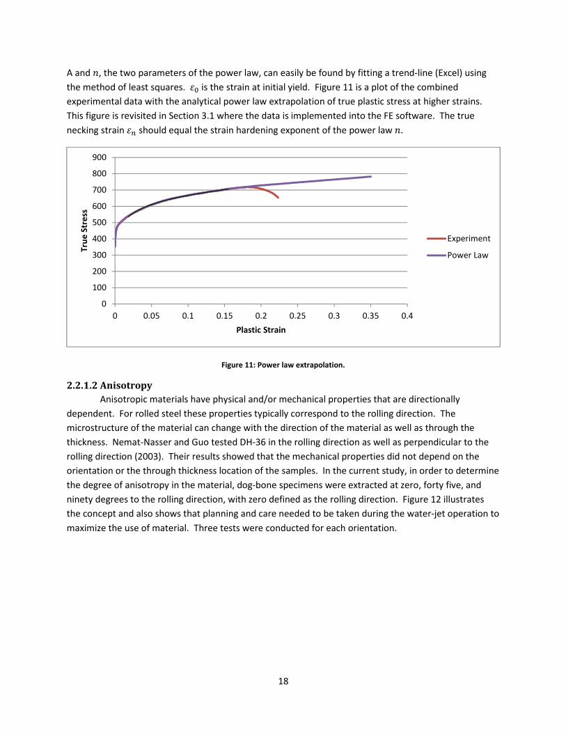
A and G, the two parameters of the power law, can easily be found by fitting a trend-line (Excel) using
the method of least squares. �� is the strain at initial yield. Figure 11 is a plot of the combined
experimental data with the analytical power law extrapolation of true plastic stress at higher strains.
This figure is revisited in Section 3.1 where the data is implemented into the FE software. The true
necking strain �� should equal the strain hardening exponent of the power law G.
Figure 11: Power law extrapolation.
2.2.1.2 Anisotropy
Anisotropic materials have physical and/or mechanical properties that are directionally
dependent. For rolled steel these properties typically correspond to the rolling direction. The
microstructure of the material can change with the direction of the material as well as through the
thickness. Nemat-Nasser and Guo tested DH-36 in the rolling direction as well as perpendicular to the
rolling direction (2003). Their results showed that the mechanical properties did not depend on the
orientation or the through thickness location of the samples. In the current study, in order to determine
the degree of anisotropy in the material, dog-bone specimens were extracted at zero, forty five, and
ninety degrees to the rolling direction, with zero defined as the rolling direction. Figure 12 illustrates
the concept and also shows that planning and care needed to be taken during the water-jet operation to
maximize the use of material. Three tests were conducted for each orientation.
0
100
200
300
400
500
600
700
800
900
0 0.05 0.1 0.15 0.2 0.25 0.3 0.35 0.4
Tru
e S
tre
ss
Plastic Strain
Experiment
Power Law

19
Figure 12: Dog-bone orientation with respect to the rolling direction.
The measurement used to quantify the amount of anisotropy is the Lankford ratio (��), where α
is the angle measured from the rolling direction. The parameter is the ratio of the strain in the width
direction to the strain in the through-thickness direction.
�� 0 B�IJ &-BKL (9)
DIC enables accurate measurement of in plane strains �M and �N. The plastic incompressibility condition
is utilized to express �., thickness reduction, as −1BKO 2 BKP/. The Lankford parameter is important in
drawing and stamping operations. A fully isotropic material will have a Lankford ratio equal to unity. If
the ratio is greater than unity it is more difficult to reduce the thickness of the material than having it
drawn from a blank. Figure 13 shows the relationship of transverse and through thickness strains for
the specimens in all three directions. The slopes of the lines correspond to the �� values. As observed
by Nemat-Nasser and Guo there is little to no anisotropy between the rolling direction (0°) and the
transverse direction (90°).
20
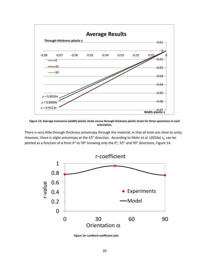
Figure 13: Average transverse (width) plastic strain versus through-thickness plastic strain for three specimens in each
orientation.
There is very little through thickness anisotropy through the material, in that all tests are close to unity.
However, there is slight anisotropy at the 45° direction. According to Mohr et al. (2010a)�� can be
plotted as a function of α from 0° to 90° knowing only the 0°, 45° and 90° directions, Figure 14.
Figure 14: Lankford coefficient plot.
y = 0.8409x
y = 0.9523x
y = 0.8024x
-0.07
-0.06
-0.05
-0.04
-0.03
-0.02
-0.01
0
0.01
-0.08 -0.07 -0.06 -0.05 -0.04 -0.03 -0.02 -0.01 0
Width plastic ε
Through-thickness plastic ε
Average Results
0
45
90
0
0.2
0.4
0.6
0.8
1
0 30 60 90
r-va
lue
Orientation α
r-coefficient
Experiments
Model

21
Abaqus, the FE software used in this project uses “anisotropic creep stress ratios” � , which can be
thought of as yield ratios to express/accept the Lankford data (Abaqus 2011).
�$$ 0 1 (10)
�&& 0 V�N1�M 2 1/�M5�N 2 16
(11)
�.. 0 V�N1�M 2 1/1�M 2 �N/
(12)
�$& 0 V 31�M 2 1/�N12�AX 2 1/1�M 2 �N/
(13)
Without having data on the out of plane shear, it is assumed �$. 0 �&. 0 1 (isotropic). The anisotroic
ratios and material orientation is assigned in abaqus when conducting the FE simulations. The
anisotropy analysis defines the vertical axis of the specimen as ‘x’ and the horizontal axis as ‘y’, a 90° rotation about the z axis.
2.2.2 Notched and Hole Specimens
A variety of specimens, other than the dog-bone specimens, are used to characterize the
dependence of the fracture locus on the type of loading and state of stress. The fracture locus is a
three-dimensional (3D) surface. The specimens are designed to give data points over a broad range of
the stress parameters η and �̅, so an accurate interpolation can be carried out.
The first type of specimen to be considered is the tensile specimen with a central hole. The dog-
bone is a standard uni-axial tension test specimen. It is not used for fracture surface calibration because
the stress state varies throughout the experiment from uni-axial tension to transverse plane strain. This
variation is due to the significant neck that develops at large strains. In order to mitigate this variation
throughout the experiment and keep a more constant stress state, specifically triaxiality, the tensile
specimen with a central hole is used (Figure 15). This feature forces the fracture to initiate at the

22
intersection of the hole and the transverse axis of symmetry of the specimen.
Figure 15: Tensile specimens with different notch radii and a central hole (Dunard and Mohr 2010a).
Testing is also carried out on similar geometries, the notched specimens. These are flat tensile
specimens with circular cutouts (Figure 15). The triaxiality within the specimen is a function of the notch
radius, thus a range of stress states can be achieved. The expression for initial triaxiality is given by:
Y 0 1 2 2Λ3√Λ& 2 Λ 2 1 (14)
where Λ 0 ln[1 2 < 14�/⁄ ] and R denotes the radius of the cutout (Y. Bai 2008). The stress state
approaches uni-axial tension (dog-bone Y 0 0.333) as the notch radius increases. It approaches plane
strain (Y 0 0.577), along the width of the specimen, as the notch radius decreases. Three different
notch radii are used, R = 20mm, R = 10mm and R = 6.67mm. The central hole and notched specimen
loading axis is always oriented along the rolling direction.
2.2.3 Punch Specimen
The punch tests performed demonstrate fracture under an equi-biaxial state of stress. The
geometry can be seen in Figure 16. The outer holes are for bolts used to clamp the outside of the
specimen into a specially designed die.

23
Figure 16: Punch specimen schematic and post test.
The tests were performed in the MTS loading machine. Sandwiched sheets of Teflon (5 at .002 in-thick)
and grease were used in between the hemispherical punch and specimen to eliminate unwanted
frictional forces that would disturb results. The apex of the dome created during the test (Figure 16) is
the most highly-stressed point where radial and circumferential stress and strain are equal to each
other.
2.2.4 Butterfly Specimen
The butterfly specimen is designed to maintain uniform stress and strain fields during
combinations of normal and tangential loading. Mohr and Oswald outlined the details of the multi-axial
testing procedure (2007).
Figure 17: Dual Actuator Loading Frame and definition of the bi-axial loading angle β (Mohr, Dunard and Kim 2010).

24
Figure 17 demonstrates the bi-axial loading angle β. In the current calibration, tests were only
conducted at the limiting cases of ! 0 0° and ! 0 90° corresponding to pure shear and transverse
plane strain respectively. The specimen geometry has changed over the years but was recently
optimized by Dunard and Mohr and can be seen in Figure 18 (2009). The geometry is optimized to
ensure fracture initiates remote from the free specimen boundaries regardless of loading angle. The
design prevents unwanted plastic deformation, high strain concentrations, crack initiation and/or
buckling. It also fulfills the obvious task of fitting the dual actuator loading frame and meeting
manufacturing constraints.
Figure 18: Optimized butterfly specimen (Dunard and Mohr 2009).
Fracture initiates at the center of the specimen and the crack propagates in a stable way toward the
boundaries in a kinematically-controlled test. During pure shear testing, the horizontal actuator is in
displacement control and the vertical actuator is in force control, maintaining a normal force of zero.
Selected images from experimental testing are included in Appendix B.
3 Numerical Simulation
3.1 Hybrid Approach
There are two main reasons numerical simulations are necessary. First, the material points where
fracture initiates are inside the specimens. It is impractical to attempt to make observations and
retrieve data from the center of a specimen in a physical test. Also, the data and parameters required
from the tests, even if fracture were to occur on the surface, are extremely complicated and can be
calculated quickly and accurately using FE software. The simulations provide perspective on the
evolution of the third invariant, von Mises stress, pressure, triaxiality and equivalent plastic strain up to
fracture initiation. The hybrid-approach used is based on the work of Dunard and Mohr (2010a).
3.2 Setup
Implicit finite element simulations were conducted using Abaqus/standard. The notched and
central-hole specimens were meshed using reduced-integration eight-node 3D solid elements (C3D8R in
the Abaqus library). In order to save on computing time, the simulations took advantage of the
symmetry of the specimen’s geometry, material properties, and loading conditions. Thus, only one eight
of the specimen, half the thickness of an upper corner, was modeled. X, Y, and Z symmetry planes were
assigned.
25
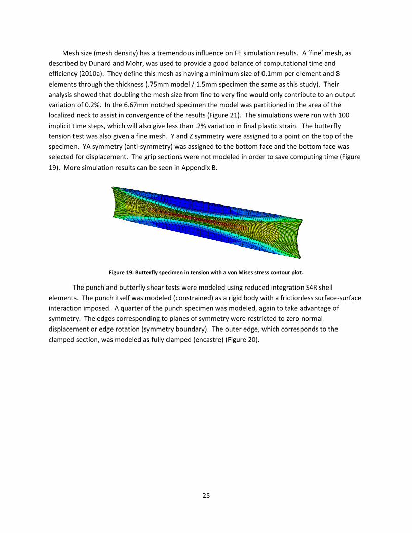
Mesh size (mesh density) has a tremendous influence on FE simulation results. A ‘fine’ mesh, as
described by Dunard and Mohr, was used to provide a good balance of computational time and
efficiency (2010a). They define this mesh as having a minimum size of 0.1mm per element and 8
elements through the thickness (.75mm model / 1.5mm specimen the same as this study). Their
analysis showed that doubling the mesh size from fine to very fine would only contribute to an output
variation of 0.2%. In the 6.67mm notched specimen the model was partitioned in the area of the
localized neck to assist in convergence of the results (Figure 21). The simulations were run with 100
implicit time steps, which will also give less than .2% variation in final plastic strain. The butterfly
tension test was also given a fine mesh. Y and Z symmetry were assigned to a point on the top of the
specimen. YA symmetry (anti-symmetry) was assigned to the bottom face and the bottom face was
selected for displacement. The grip sections were not modeled in order to save computing time (Figure
19). More simulation results can be seen in Appendix B.
Figure 19: Butterfly specimen in tension with a von Mises stress contour plot.
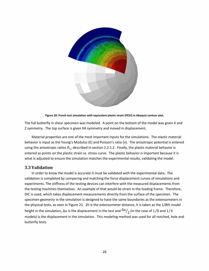
The punch and butterfly shear tests were modeled using reduced integration S4R shell
elements. The punch itself was modeled (constrained) as a rigid body with a frictionless surface-surface
interaction imposed. A quarter of the punch specimen was modeled, again to take advantage of
symmetry. The edges corresponding to planes of symmetry were restricted to zero normal
displacement or edge rotation (symmetry boundary). The outer edge, which corresponds to the
clamped section, was modeled as fully clamped (encastre) (Figure 20).
26
Figure 20: Punch test simulation with equivalent plastic strain (PEEQ in Abaqus) contour plot.
The full butterfly in shear specimen was modeled. A point on the bottom of the model was given X and
Z symmetry. The top surface is given XA symmetry and moved in displacement.
Material properties are one of the most important inputs for the simulations. The elastic material
behavior is input as the Young’s Modulus (E) and Poisson’s ratio (ν). The anisotropic potential is entered
using the anisotropic ratios � described in section 2.2.1.2. Finally, the plastic material behavior is
entered as points on the plastic strain vs. stress curve. The plastic behavior is important because it is
what is adjusted to ensure the simulation matches the experimental results, validating the model.
3.3 Validation
In order to know the model is accurate it must be validated with the experimental data. The
validation is completed by comparing and matching the force displacement curves of simulations and
experiments. The stiffness of the testing devices can interfere with the measured displacements from
the testing machines themselves. An example of that would be strain in the loading frame. Therefore,
DIC is used, which takes displacement measurements directly from the surface of the specimen. The
specimen geometry in the simulation is designed to have the same boundaries as the extensometers in
the physical tests, as seen in Figure 21. 2h is the extensometer distance, h is taken as the 1/8th model
height in the simulation, ∆= is the displacement in the test and ∆= 2- (in the case of 1 8⁄ and 1 4⁄
models) is the displacement in the simulation. This modeling method was used for all notched, hole and
butterfly tests.
27
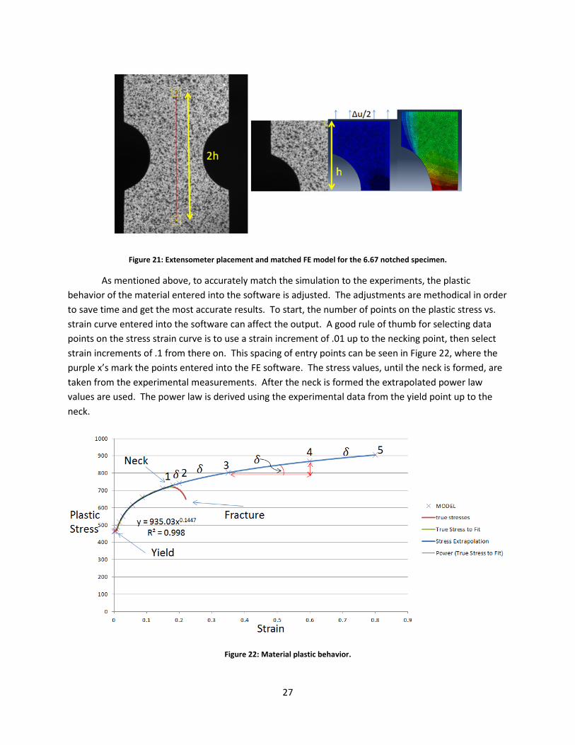
Figure 21: Extensometer placement and matched FE model for the 6.67 notched specimen.
As mentioned above, to accurately match the simulation to the experiments, the plastic
behavior of the material entered into the software is adjusted. The adjustments are methodical in order
to save time and get the most accurate results. To start, the number of points on the plastic stress vs.
strain curve entered into the software can affect the output. A good rule of thumb for selecting data
points on the stress strain curve is to use a strain increment of .01 up to the necking point, then select
strain increments of .1 from there on. This spacing of entry points can be seen in Figure 22, where the
purple x’s mark the points entered into the FE software. The stress values, until the neck is formed, are
taken from the experimental measurements. After the neck is formed the extrapolated power law
values are used. The power law is derived using the experimental data from the yield point up to the
neck.
Figure 22: Material plastic behavior.

28
The adjustment, in order to match simulation to experiment, takes place between the points labeled 1
thru 5. The slopes (δ) between the points are calculated. These δ’s are then used as ‘triggers’ to adjust
the plastic stress up or down. The force displacement curve from the simulation is compared to that of
the actual experiment. If the force in the simulation is too low the plastic stress is slightly increased by
these triggers and the simulation is re-executed. The process repeats until the force displacement
curves match. The outcome is shown using Figure 23. The plot shows, for the central-hole tests, the
two experimental force displacement curves as well as the ensuing simulations until a match was
reached. In this case, 9 iterations were needed. Also, the 6.67 notch test and simulation curve are
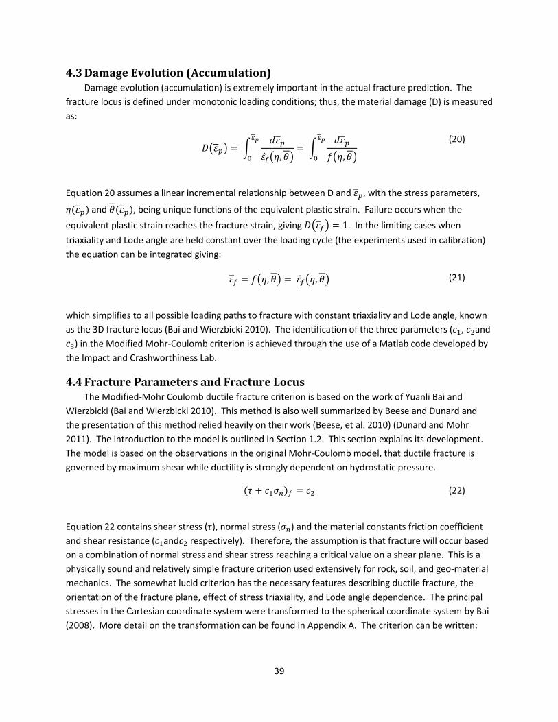
shown in Figure 24 to give a clear view of the match. All simulations need to be matched in this way to
ensure accurate data is coming from the simulation. More plots are included in Appendix B.
Figure 23: Force displacement simulation test series for the central hole specimen.
-2
0
2
4
6
8
10
12
14
0 0.5 1 1.5 2 2.5 3
Fo
rce
[k
N]
Displacement [mm]
t_1
t_2
Simulation
Simulation_2
Simulation_3
Simulation_4
Simulation_5
Simulation_6
Simulation_7
Simulation_8
Simulation_9
Simulation_10

29
Figure 24: Force displacement simulation comparison for the 6.67 notched specimen.
The punch test is a special case. Due to the geometry and the out of plane deformations 3-D
vice 2-D DIC is required (section 2.1.2). For the two cameras to capture images during the test an angled
mirror is placed under the specimen and its clamping frame. The cameras can then be directed at this
mirror giving them a view of the underside of the test. Figure 25 shows the 3-D DIC displacement
contour plot at a time close to fracture. Displacements shown are in the direction of the punch’s path.
This is an image from one of the two cameras used during the test. The circles appear to be off centered
because the camera is not perfectly centered on the specimen. It is not centered because the cameras
need different perspectives of the specimen to capture the relative displacement and thus the third
dimension, they are not perfectly centered on the test area. Using the software, points on the image
can be selected, and displacements or strains can be extracted for that point over the duration of the
test.
Figure 25: 3-D DIC displacement contour plot.
-2
0
2
4
6
8
10
12
0 0.5 1 1.5 2 2.5
Fo
rce
[k
N]
Displacement [mm]
t_1
t_2
Simulation

30
Two punch tests were executed. In the second test, due to the high ductility of the material, the
painted speckle pattern de-laminated from the specimen surface before fracture, which restricted the
use of DIC in that test. The degraded paint near the fracture point can be seen in Figure 26.
Figure 26: Punch test setup and specimen after fracture.
As stated above, displacement measurements can be taken from the MTS loading frame instead of using
DIC. However, that data is affected by the behavior of all the devices located between the specimen
and the measurement device. Since DIC data for the second punch test could not be obtained, the force
displacement curve with MTS displacement data was taken and compared for the first and second test,
simply to confirm repeatability. The punch test is a very repeatable test, which is confirmed in Figure 27
by the series ‘Test_1’ and ‘Test_2’. Also shown in the figure, the FE simulation was matched to the 3-D
DIC plot for the first test, showing a good match. Notice the simulation goes past the actual fracture
displacement. This overshoot is not incorrect and is discussed further in section 3.4
Figure 27: Punch force displacement curve.
-10
0
10
20
30
40
50
60
70
80
90
-5 0 5 10 15 20
Fo
rce
[k
N]
Displacement [mm]
Punch
Test_1
Test_2
3D_DIC_Test1
Simulation

31
3.4 Data Analysis
Once the simulations are validated the history responses of the pertinent parameters can be easily
extracted from the FE software. All stages of the experiment are captured in the simulations including
elastic deformation, yield, plastic deformation, diffuse necking, onset of fracture, and final fracture
(rupture). This evolution can be seen in the experimental stress strain curve of a dog-bone specimen
(Figure 28).
Figure 28: Typical stress strain curve.
The values that describe the state of stress and equivalent plastic strain are changing throughout the
experiment and simulation. The final values used in the fracture model are not the numbers at final
rupture. If they were, the process of pulling the correct data from the simulation would be much easier,
in that the displacement at rupture could just be read at the start of the steep drop in the stress strain
plot. The actual fracture initiation is located somewhere between neck formation and rupture, the red
circle in Figure 28. The process for finding this point involves going back to the images, taken for DIC,
and finding the point in time where the first surface discontinuity occurs. The corresponding
displacement in the given test will give the exact point in the simulation where the stress states for
calibration are taken. Figure 29 shows the transition and identification of onset of fracture for the
butterfly specimen in tension. The identification of onset to fracture is crucial because plastic strain can
change, especially in a ductile material, on the order of 10%. The images labeled 1 to 4 are the first four
images, taken over 4 seconds, where onset of fracture is observed. A zoomed in image of the fracture
area is included. The sub-figure labeled 5 is taken later in time when fracture is much more evident.
32
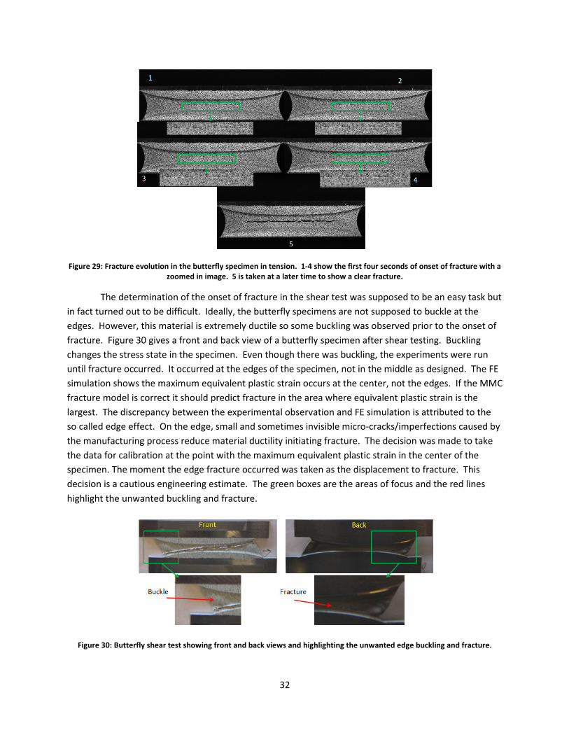
Figure 29: Fracture evolution in the butterfly specimen in tension. 1-4 show the first four seconds of onset of fracture with a
zoomed in image. 5 is taken at a later time to show a clear fracture.
The determination of the onset of fracture in the shear test was supposed to be an easy task but
in fact turned out to be difficult. Ideally, the butterfly specimens are not supposed to buckle at the
edges. However, this material is extremely ductile so some buckling was observed prior to the onset of
fracture. Figure 30 gives a front and back view of a butterfly specimen after shear testing. Buckling
changes the stress state in the specimen. Even though there was buckling, the experiments were run
until fracture occurred. It occurred at the edges of the specimen, not in the middle as designed. The FE
simulation shows the maximum equivalent plastic strain occurs at the center, not the edges. If the MMC
fracture model is correct it should predict fracture in the area where equivalent plastic strain is the
largest. The discrepancy between the experimental observation and FE simulation is attributed to the
so called edge effect. On the edge, small and sometimes invisible micro-cracks/imperfections caused by
the manufacturing process reduce material ductility initiating fracture. The decision was made to take
the data for calibration at the point with the maximum equivalent plastic strain in the center of the
specimen. The moment the edge fracture occurred was taken as the displacement to fracture. This
decision is a cautious engineering estimate. The green boxes are the areas of focus and the red lines
highlight the unwanted buckling and fracture.
Figure 30: Butterfly shear test showing front and back views and highlighting the unwanted edge buckling and fracture.

33
3.5 New Shear Specimen
Due to the problems experienced with the butterfly specimen used for shear testing, a new type of
specimen was examined to achieve pure shear all the way up to the onset of fracture. The new
specimen can be seen in Figure 31.
Figure 31: New Shear Specimen (inches).
The specimen is commonly used in industry and is meant to more easily achieve shear by utilizing a
simple geometry which can be tested on a standard loading frame. It is worth noting the measurements
shown are in inches and the specimen was created with a thickness of 1.5mm, in order to be consistent
with the other specimens in this analysis. The test was conducted using the MTS loading frame. The
holes shown on the drawing were not machined because grips are used as the mounting apparatus on
the MTS. In future testing a slightly wider grip section should be designed into the specimen (as seen in
Figure 15) to mitigate any unwanted stress states near the grips; although, in the 2-D DIC analysis of the
test there were not errant strains observed near the grips, so this test was still valid.
The experiments and data analysis were successfully conducted with very repeatable results.
One observation is that the specimen needs to be mounted perfectly, aligned in exact symmetry,
specifically in the vertical direction. Any misalignment will cause the specimen to take on a twisting
action negating the desired pure shear scenario and putting the gage section into tension and/or torsion
and thus creating an unwanted stress state and neck.
The finite element simulations had great correlation with the experimental force displacement
curve. However, the specimen fractured at a much lower triaxiality and Lode angle then the safe
estimate taken from the butterfly specimen simulations. This discrepancy is discussed further in section
4.2 and resulted in this new specimen’s data not being used in the MMC model calibration

34
4 Modified Mohr-Coulomb Fracture Criterion
4.1 Data Collection and Calibration
With simulations complete the next step in the process is to determine the equivalent plastic strain
as a function of triaxiality and Lode angle at the onset of fracture for all the specimens (more
background is included in Appendix A). The equivalent plastic strain (��̅� or PEEQ in Abaqus) at the onset
of fracture is simply known as the fracture strain (��). The equivalent plastic strain, third invariant, von
Mises stress, and pressure can all be defined as history outputs and taken directly from the simulation
results. Stress triaxiality and Lode angle are calculated from these outputs. Stress triaxiality, also known
as the dimensionless hydrostatic pressure, is the ratio of the mean stress (��) to the equivalent stress
(��). It is the normalized pressure and gives the average level of stress and its distribution along all
principal directions.
Y 0 �� ��- 0 −:-̀ (15)
The mean stress can be written as the negative pressure (-p) and the equivalent stress can be written as
the von Mises stress (q).
: 0 � 0 <�1�/ (16)
` 0 V32 1a: a/
(17)
S is the deviatoric stress. The dimensionless Lode angle parameter is defined by �̅ 0 1 − 6� d- so that -
1<�̅<1, where cos(3θ)=1�./��/. with � being the Lode angle. Sometimes the symbol f is used to
represent the normalized third invariant.
f 0 1�./��/. = 1�/`/. (18)
r and �. both represent the third invariant of the stress deviator tensor. The dimensionless (normalized)
Lode angle is used in the model and is solved for in the form:
�̅ 0 1 − 2d arccos1f/ (19)
All simulations were run until the complete failure (rupture) of the specimen. Each series of
images for a given experiment is analyzed to find the image corresponding to the onset of fracture.
From the image numbering in the DIC software the exact displacement at fracture initiation is
interpreted. In the FE simulation, the element with the maximum equivalent plastic strain at the onset

35
of fracture is detected and recorded. This element is where the data describing the state of stress and
strain is taken. Equivalent plastic strain is plot against Lode angle and triaxiality. The equivalent plastic
strain vs. triaxiality can be seen in Figure 32 and the equivalent plastic strain vs. Lode angle can be seen
in Figure 33. The new shear specimen (Section 3.5) was not used in the final calibration.
Figure 32: Equivalent plastic strain and triaxiality.

36
Figure 33: Equivalent plastic strain and Lode angle.
The displacement at onset of fracture is then used with the FE data to identify the onset of fracture on
the plots, the red “x” shows where the onset of fracture occurred. The data is organized as seen in
Table 1. Two tests were executed for each specimen but only one value of strain is given in the table.
Only one value of �� is shown in the table because the displacement to fracture varied by less than one
percent between similar specimens. Thus, the tests were very repeatable. The lower displacement
value, vice an average, was used to obtain the fracture strain from the simulations. The displacement to
fracture of the punch specimen varied by about 6 percent but only one of the experiments had useable
3-D DIC data, as discussed in section 3.3.
Table 1: Parameters used in model calibration.
Table of Parameters � �l mn Specimen
0.775 0.164 0.793 notched 6.67
0.762 0.169 0.829 notched 10
0.732 0.185 0.839 notched 20
0.349 0.953 0.925 central hole
-0.010 -0.028 1.368 butterfly shear
0.794 0.155 0.857 butterfly tension
0.667 -0.979 0.805 punch

37
4.2 New Shear Specimen Discussion
As stated in section 3.5 the new shear specimen experiment had very repeatable results. Also, the
force displacement curve of the experiment and simulation showed good correlation; however, the
specimen fractured at a much lower triaxiality and Lode angle then the safe estimate taken from the
butterfly specimen simulations, even though the stress states should have been similar.
When looking at the simulation results, in the gage section of the specimen the triaxiality and Lode
angle were similar to those of the butterfly specimen in shear. Thus, the gage section was in pure shear.
The problem is that during the tests sharp edges form outside of the gage section, this can be seen in
Figure 34 which shows the specimen prior to testing, half way through the test, one second before
fracture, and one second after fracture.
Figure 34: New shear specimen experiment prior to testing, mid-test ‘half’, one second prior to fracture, and one second
after fracture.
It is difficult to tell for sure from the experimental data but it is possible that fracture initiates at
these edges, which would make the test invalid. Ideally, fracture would initiate at the center of the gage
section where the desired pure shear stress state is achieved. The FE simulations give more evidence to
believe that fracture initiates outside of the gage section. In the simulation, at the displacement of
failure the highest equivalent plastic strain is observed at one of these edges (Figure 35).
Figure 35: FE simulation PEEQ contour plot at the displacement of fracture, showing the maximum point of equivalent plastic
strain in the edge section not the gage section. The face shown is the middle of the specimen.

38
Figure 36 shows equivalent plastic strain to fracture as a function of triaxiality and Lode angle. The new
shear specimen’s history is shown at the point in the gage section with the highest equivalent plastic
strain (labeled ‘new shear gage’) and the point at the edge (labeled ‘new shear edge’) with the highest
overall equivalent plastic strain in the specimen. From the plots it becomes clear that fracture in the
new shear specimen seams to initiate early when looking at the gage section history. However, when
looking at the edge, it fails as predicted from different specimens. These results led to the new shear
specimen not being used in the calibration.
Figure 36: Plots of equivalent plastic strain as a function of triaxiality and Lode angle.
The butterfly specimen in shear buckled causing fracture to initiate early. Thus, this displacement
to fracture had to be used as a conservative lower bound. A follow on study, or other studies of very
ductile materials, may use an older version of the butterfly specimen which is not as good in combined
loading but will be more resistant to buckling in pure shear (Figure 37). In the case of DH-36, the
fracture strain was clearly linked to triaxiality and follow on tests with the older version of the butterfly
specimen may show even more dependence.
Figure 37: Alternate butterfly specimen for future testing.
39
4.3 Damage Evolution (Accumulation)
Damage evolution (accumulation) is extremely important in the actual fracture prediction. The
fracture locus is defined under monotonic loading conditions; thus, the material damage (D) is measured
as:
@5��6 0 o B����̂5Y, �6Kq
� 0o B��(5Y, �6Kq�
(20)
Equation 20 assumes a linear incremental relationship between D and ��, with the stress parameters, Y1��/ and �1��/, being unique functions of the equivalent plastic strain. Failure occurs when the
equivalent plastic strain reaches the fracture strain, giving @5��6 0 1. In the limiting cases when
triaxiality and Lode angle are held constant over the loading cycle (the experiments used in calibration)
the equation can be integrated giving:
�� 0 (5Y, �6 0 ��̂5Y, �6 (21)
which simplifies to all possible loading paths to fracture with constant triaxiality and Lode angle, known
as the 3D fracture locus (Bai and Wierzbicki 2010). The identification of the three parameters (#$, #&and #.) in the Modified Mohr-Coulomb criterion is achieved through the use of a Matlab code developed by
the Impact and Crashworthiness Lab.
4.4 Fracture Parameters and Fracture Locus
The Modified-Mohr Coulomb ductile fracture criterion is based on the work of Yuanli Bai and
Wierzbicki (Bai and Wierzbicki 2010). This method is also well summarized by Beese and Dunard and
the presentation of this method relied heavily on their work (Beese, et al. 2010) (Dunard and Mohr
2011). The introduction to the model is outlined in Section 1.2. This section explains its development.
The model is based on the observations in the original Mohr-Coulomb model, that ductile fracture is
governed by maximum shear while ductility is strongly dependent on hydrostatic pressure.
1� 2 #$��/� 0 #& (22)
Equation 22 contains shear stress (�), normal stress (��) and the material constants friction coefficient
and shear resistance (#$and#& respectively). Therefore, the assumption is that fracture will occur based
on a combination of normal stress and shear stress reaching a critical value on a shear plane. This is a
physically sound and relatively simple fracture criterion used extensively for rock, soil, and geo-material
mechanics. The somewhat lucid criterion has the necessary features describing ductile fracture, the
orientation of the fracture plane, effect of stress triaxiality, and Lode angle dependence. The principal
stresses in the Cartesian coordinate system were transformed to the spherical coordinate system by Bai
(2008). More detail on the transformation can be found in Appendix A. The criterion can be written:

40
�� 0 #& rV1 2 #$&3 #s" td6 − �u 2 #$ vY 2 13 ">G td6 − �uwxH$
(23)
The equation, in the form above, is expressed in terms if equivalent fracture stress (��). It needs to be
transformed into the mixed stress-strain space so that the experiments, measured in equivalent fracture
strain (��) can be incorporated. Assuming von Mises yield condition a simple power law (as seen in
section 2.2.1.1) � 0 1�� 2 ��/� , can be used to express equivalent stress as equivalent strain, yielding:
�� 0 y#& rz1 2 #$&3 cos v�d6 w 2 #${Y 2 13 ">G v�d6 w|x}H$�
(24)
Equation 24 describes a yield surface for a quadratic yield condition. A “non-quadratic” yield condition
was proposed by Bai (2008) which is modified by the Lode angle parameter using the hardening law:
� 0 �� ~#. 2 √32 − √3 11 − #./ v"8# v�d6 w − 1w� (25)
By adding the parameter #. various shapes of the yield surface can be formed. This feature is made
clear in Figure 38, where a von Mises yield criterion is shown by #. 0 1 and a Tresca yield condition
shown by #. 0 √3 2- .
Figure 38: Effect of �� on the yield surface (Beese, et al. 2010).
Now, with the elimination of the equivalent stress (�) the MMC criterion becomes:

41
�� 0 y#& ~#. 2 √32 − √3 11 − #./ v"8# v�d6 w − 1w� ∙ rz1 2 #$&3 cos v�d6 w 2 #${Y 2 13 ">G v�d6 w|x}H$�
(26)
4.4.1 2D Plane Stress Model
The model can be simplified for the plane stress condition (�. 0 0) (Wierzbicki and Xue 2005)
(Bai and Wierzbicki 2008). In these cases triaxiality and Lode angle can be expressed as:
f 0 cos13�/ 0 −272 Y CY& − 13E 0 sin1d2 �/ (27)
Using this relationship, equations 26 and 27 can be combined and the plane stress fracture locus is
described by:
�� 0 y#& (. r{V1 2 #$&3 ($|2 #$ CY 2 (&3 Ex}H$�
(28)
($ 0 #s" ~13 ;�#">G �−272 Y CY& − 13E�� (29)
(& 0 ">G ~13 ;�#">G �−272 Y CY& − 13E�� (30)
(. 0 #. 2 √32 − √3 11 − #./ C1($ − 1E (31)
The parameters #$ and #. define the contour and shape of the fracture locus and #&adjusts the size. By
assuming plane stress the problem can be solved in the 2D plane. This 2D analysis is helpful in getting a
starting point if the original 3D fitting is unsuccessful. In fitting DH-36, the fracture locus has a simple
shape and fitting the 3D plot was not a problem.
4.4.2 3D Fracture Locus
A Matlab code, developed by the Impact and Crashworthiness lab at MIT, is used to calculate the
best fit for the three parameters. The code uses the Matlab function fmincon which finds a constrained
minimum of a function of several values. It looks for the local minimum to a solution guessed by the
user using bounds also input by the user. Defining these initial conditions is where the 2D method may
be useful. The function the code minimizes is defined by the difference between the experimental
calibration results and the equation for the equivalent strain at fracture (��) surface. The effects of the

42
parameters on the fracture locus were studied in depth by Bai and Wierzbicki (2008). The calibrated 3D
Modified Mohr-Coulomb fracture locus for DH-36 steel can be seen in Figure 39.
Figure 39: DH-36 MMC 3D Fracture Locus.
It is worth noting there is also a more complicated four parameter MMC model. The fourth parameter is #�M. This parameter, like#., characterizes the dependence of the plasticity model on the first and third
stress invariants. The parameter #�M controls the asymmetry of the fracture envelope with respect to
the planef 0 0 (Dunard and Mohr 2011). Industry would strive for the lowest amount of parameters
possible to make calibration faster and simulations less costly. With the extremely tight fit seen in
Figure 39, it is clear the three parameter MMC fracture locus is sufficient for DH-36. Table 2 summarizes
the MMC parameters for DH-36.
Table 2: DH-36 MMC Parameters
A [Mpa] 904
n 0.1387
c1 0.0575
c2 471.2978
c3 0.866
R2
.9968

43
5 Conclusions and Further Studies Calibration of the Modified Mohr Coulomb fracture model for DH-36 steel was successful. There
are some comments that need to be made on the results and future study. First, there was some
variance seen in the basic stress strain characteristics of the material when comparing the results of this
study with those of Nemat-Nasser and Guo and Yuanli Bai (Nemat-Nasser and Guo 2003) (Y. Bai 2008).
It is possible that there may be differences in the material as delivered from the producer or some other
outside influence to the characteristics. In agreement with the works listed, there was very little
anisotropy in the material and somewhat small Lode angle dependence. The fracture strain was clearly
linked to triaxiality and follow on tests may show even more dependence.
A suggestion for future execution of the calibration process would be to use even fewer specimens.
The three notched specimens, 6.67, 10, and 20, and the butterfly specimen in tension give very similar
positions on the fracture surface. The multiple bunched points as seen in Figure 39 do not add much
more clarity to the solution and only make it more difficult for the minimization function to find a
solution. For different materials these specimens may have better spacing and give a better solution to
the optimization. However, if machining and testing cost is a concern one notch specimen would suffice.
Further studies may benefit from testing on the butterfly specimen in combined loading to better
validate the model. Nemat-Nasser and Guo have already produced great results on DH-36 over a wide
range of strain rates and temperatures (Nemat-Nasser and Guo 2003). However, further dynamic
testing could make the current MMC model more robust. The Impact and Crashiworthiness Lab has
developed a new tool for high strain rate fracture testing which could be useful in studying DH-36 and
polyurea (Dunard, Gary and Mohr 2011). As mentioned in the introduction, the motivation for
calibrating DH-36 was achieving the first step in better modeling its use with polyurea. More testing of
polyurea could be incorporated with these results to better optimize design and application of DH-36
with polyurea. This properly calibrated MMC model is a great first step in conducting accurate and
inexpensive analysis techniques.

44
References
Abaqus. ABAQUS analysis user's manual version 6.11. Providence (RI): Dassault Systemes, 2011.
Amini, M.R., A.V. Amirkhizi, and S. Nemat-Nasser. "Numerical modeling of response of monolithic and
bilayer plates to impulsive loads." International Journal of Impact Engineering, 2010d: 90-102.
Amini, M.R., and S. Nemat-Nasser. "Micromechanisms of ductile fracturing of DH-36 steel plates." Int J
Fract 162, 2010c: 205-217.
Amini, M.R., J. Isaacs, and S. Nemat-Nasser. "Investigation of effect of polyurea on response of steel
plates." Mechanics of Materials, 2010b: 628-639.
Amini, M.R., J. Simon, and S. Nemat-Nasser. "Numerical modeling of effect of polyurea on response of
steel plates to impulsive loads in direct pressure-pulse experiments." Mechanics of Materials,
2010a: 615-627.
Amirkhizi, A.V., J. Isaacs, J. McGee, and S. Nemat-Nasser. " An experimentally-based viscoelastic
constitutive model for polyurea, including pressure and temperature effects." Philosophical
Magazine and Philosophical Magazine Letters, 2006: 5847-5866.
ASTM. "ASTM." Standard Test Methods for Tension Testing of Metallic Materials [Metric] E 8M - 04. 10
10, 2001. www.astm.org (accessed 01 31, 2005).
Bai, Y. Effect of Loading History on Necking and Fracture. Thesis, Cambridge: MIT, 2008.
Bai, Y, and T Wierzbicki. "Application of extended Mohr-Coulomb criterion to ductile fracture." Int J Fract
161, 2010: 1-20.
Bai, Y., and T. Wierzbicki. "A new model of metal plasticity and fracture with pressure and Lode."
International Journal of Plasticity, 2008: 1071-1096.
Bao, Y. "On fracture locus in the equivelent strain and stress triaxiality space." International Journal of
Mechanical Sciences, 2004: 81-98.
Bao, Y, and T Wierzbicki. "On fracture locus in the equivelent strain and stress triaxiality space."
International Journal of Mechanical Sciences, 2004: 81-98.
Beese, Allison, Luo Meng, Yaning Li, Yuanli Bai, and T Wierzbicki. "Partially coupled anisotropic fracture
model for aluminum sheets." Engineering Fracture Mechanics, 2010.
Crane, David. "U.S. Military Testing Spray-On Polymer Armor." Defense Review. May 10, 2004.
http://www.defensereview.com/us-military-testing-spray-on-polymer-armor/ (accessed
November 02, 2011).

45
Dunard, M, and D Mohr. "Hybrid experimental-numerical analysis of basic ductile fracture experiments
for sheet metals." International Journal of Solids and Structures (International Journal of Solids
and Structures), 2010a: 1130-1143.
Dunard, M, and D Mohr. Report 216: Predicting Ductile Fracture in Advanced High Strength Steel Sheets:
Comparison of Two approaches. Impact and Crashworthiness Lab, 2010b.
Dunard, M., and D. Mohr. Report No. 199: Optimized Specimen for the Fracture Testing of. Report No.
199, Cambridge: Impact and Crashworthiness Lab, 2009.
Dunard, Matthieu, and Dirk Mohr. "On the Predictive Capabilities of the Shear Modified Guerson and
the Modified-Mohr Coulomb Fracture Models over a Wide Range of Stress Triaxialities and Lode
Angles." Journal of the Mechanics and Physics of Solids Volume 59 Issue 7, 2011: 1374-1394.
Dunard, Matthieu, Gerard Gary, and Dirk Mohr. A New Device for High Strain Rate Frature Testing. No.
224, Cambridge: Impact and Crashworthiness Lab, 2011.
Gurson, AL. "Continum Theory of Ductile Rupture by Void Nucleation and Growth: Part I Yield Criteria
and Flow Rules for Porous Ductile Media." Eng. Mater. Technology, 1977: 2-15.
Hill, R. "A theory of the yielding and plastic flow of anisotropic metals." Proc. R. Soc. Lond., 1948: 281-
297.
Johnson, G.R., and W.H. Cook. "Fracture characteristics of three metals subjected to various."
Engineering Fracture Mechanics, 1985: 31-48.
Kalpakjian, Serope, and Steven R. Schmid. Manufacturing Engineering and Technology Fourth Edition.
Saddle River: Prentice-Hall, 2001.
Klepaczko, J.R., A. Rusinek, J.A. Rodriguez-Martinez, R.B. Pecherski, and A. Arias. "Modelling of thermo-
viscoplastic behaviour of DH-36 and Weldox 460-E." Mechanics of Materials 41, 2009: 599-621.
Lassance, D, D Fabrègue, F Delannay, and Pardoen, T. "Mircomechanics of room and high temperature
fracture in 6xxx Al alloys." Prog. Mater. Sci. 52 (1) (Prog. Mater. Sci. 52), 2007: 62-129.
Matthews, William. "Army News." Army Times. May 03, 2004.
http://www.armytimes.com/legacy/new/0-ARMYPAPER-2851089.php (accessed November 02,
2011).
McClintock, FA. "A criterion for ductile fracture by the growth of holes ." Transactions of the ASME, J.
Appl. Mech., 1968: 363-371.
Mirone, G. "Role of stress triaxiality in elastoplastic characterization and ductile failure prediction."
Engineering Fracture Mechanics, 2007: 1203-1221.
Mohr, D, and S Henn. "Calibration of Stress-triaxiality Dependent Crack Formation Criteria: A New
Hybrid Experimental-Numerical Method." Experimental Mechanics, 2007: 805-820.

46
Mohr, D., and M. Oswald. "A New Experimental Technique for the Multi-axial Testing." Experimental
Mechanics, 2008: 65-77.
Mohr, D., and M. Oswald. "A New Experimental Technique for the Multi-axial Testing." Experimental
Mechanics, 2007: 65-77.
Mohr, D., M. Dunard, and Keun-Hwan Kim. "Evaluation of associated and non-associated quadratic
plasticity models." International Journal of Plasticity, 2010.
Nasser-Nemat, S, W.J. Kang, J.D. McGee, W.-G. Guo, and J.B. Isaacs. "Experimental investigation of
energy-absorption characteristics of components of sandwich structures." International Journal
of Impact Engineering, 2006: 1119-1146.
Nemat-Nasser, Sia, and Wei-Gup Guo. "Thermomechanical Response of DH-36 structural steel over a
wide range of strain rates and temperatures." Mechanics of Materials 35, 2003: 1023-1047.
"Part 2: Rules for Materials and Welding." ABS Steel Vessel Rules. Houston: American Bureau of
Shipping, January 01, 2012.
Rice, JR, and DM Tracey. "On the ductile enlargement of voids in triaxial stress fields." Mech. Phys. Solids
17, 1969: 210-217.
Sayed, Teamer EL, Willis Mock, Alejandro Mota, Fernando Fraternali, and Michael Ortiz. "Computational
assessment of ballistic impact on a high strength." Comput. Mech., 2009: 525-534.
Shim, J., and D. Mohr. "Punch indentation of polyurea at different loading velocities: Experiments and
numerical simulations." Mechanics of Materials, 2011b: 349-360.
Shim, J., and D. Mohr. "Rate dependent finite strain constitutive model of polyurea." International
Journal of Plasticity, 2011a: 868-886.
Teng, X., T. Wierzbicki, and M. Huang. "Ballistic resistance of double-layered armor plates." International
Journal of Impact Engineering, 2008: 870-884.
Weinberg, K., A. Mota, and M. Ortiz. "A variational constitutive model for porous metal plasticity."
Comput. Mech., 2006: 142-152.
Wierzbicki, T, and D Mohr. Research Proposal to establish the Industrial Fracture Consortium 2011-2013.
Research Proposal, Cambridge: Impact and Crashworthiness Lab, 2010.
Wierzbicki, T, and L Xue. Report 136: On the Effect of the Third Invariant of the Stress Deviator on Ductile
Fracture. Inpact and Crashworthiness Lab, 2005.
Xue, L. "Damage accumulation and fracture initiation in uncracked ductile solids subjected to triaxial
loading." International Journal of Solids and Structures, 2007: 5163-5181.

47
Xue, L. "Stress based fracture envelope for damage plastic solids." Engineering Fracture Mechanics,
2009: 419-438.
Xue, Liang, Willis Mock, and Ted Belytschko . "Penetration of DH-36 Steel Plates With and Without
Polyurea Coating." Mechanics of Materials, 2010: 981-1003.

48
Appendix A: Theory – Stress States This section assumes some background in stress mechanics. It is meant to clarify some
parameters in this paper, especially because different symbols are used in the referenced literature. This
section relays known mechanics knowledge but also relies heavily on the explanations in the papers of
Bai and Beese (Beese, et al. 2010) (Bai and Wierzbicki 2010).
If assumed isotropic, a material can be modeled in terms of the three stress invariants of the
cauchy stress tensor [σ], which, as the name implies, will have the same value regardless of the
coordinate system orientation. The first, second and third stress invariants of the deviatoric stress
tensor [S] are defined respectively by,
First Invariant 0 : 0 �$ 0 −�� 0 − $. <�1[�]/ 0 − $. 1�$ 2 �& 2 �./
Second Invariant 0 ` 0 �& 0 �� 0 �.& [a] ∶ [a] 0 �$& [1�$ − �&/& 2 1�& − �./& 2 1�. − �$/&] Third Invariant � 0 �. 0 1�& [a] ∙ [a] ∶ [a]/$ .- 0 �&�& det1[a]/�$ .- 0 �&�& 1�$ − ��/1�$ − ��/1�$ − ��/�$ .-
[S]0 [�] 2 :[�] 0 [�] − t��1[�]/. u [�] �� is the mean stress, �$, �& and �. are the principal stresses and [I] is the identity tensor. Stress
triaxiality, also known as the dimensionless hydrostatic pressure, is the ratio of the mean stress �� to
the equivalent stress ��.
Y 0 −:̀ 0 �� ��-
The symbol f is used, for convenience, to represent the normalized third invariant.
f 0 C�̀E. 0 cos13�/
The dimensionless Lode angle parameter (�̅) is defined and used so that -1<�̅<1. With � as the Lode
angle:
cos13�/ 0 1�./��/.
�̅ 0 1 − 6� d- 0 1 − 2d arccos1f/
The following describes the transformation of MC to the space of ��, Y, and �̅ as discussed in
section 4.4. The state of stress is fully defined by the principal stresses �$, �& and �.. Taking an
arbitrary cutting plane, defined by the unit normal vector )$, )& and )., the shear and normal stress can
be written:

49
� 0 z)$&)&&1�$ − �&/& 2 )&&).&1�& − �./& 2 ).&)$&1�. − �$/&
�� 0 )$&�$ 2 )&&�& 2 ).&�.
As described above, fracture initiates when a combination of normal stress(��) and shear stress(�) reach
a critical value on a shear plane:
1� 2 #$��/� 0 #&
By combining the equations for normal stress and shear stress into the equation above and maximizing
the left hand side with respect to the components of the defined unit normal vector ()), the orientation
of the fracture plane can be found. Using the Lagrange multiplier technique, the direction cosines of the
maximum, intermediate and minimum principal stresses are defined by:
)$& 0 1z1 − #$& − #$/&1 2 1z1 − #$& − #$/&
)&. 0 0
).& 0 11 2 1z1 − #$& − #$/&
By combining the six equations above the MC criterion can be described in the space of principal
stresses.
As stated in Section 4.4, Bai transformed the fracture surface from the Cartesian coordinate
system to the Spherical coordinate system as illustrated in Figure 40 (Y. Bai 2008).
Figure 40: The coordinate systems in the space of Principal Stresses (Beese, et al. 2010) (Bai and Wierzbicki 2010)

50
The transformation equations are:
�$ 0 �� 2 "$ 0 �� 2 23�� cos1�/ 0 �1 2 2cos�3Y ���
�& 0 �� 2 "& 0 �� 2 23�� cos C23d − �E 0 r1 2 2cos123d − �/3Y x ��
�. 0 �� 2 ". 0 �� 2 23�� cos C43d − �E 0 r1 2 2cos143d − �/3Y x ��
The transformed form of the MC fracture criterion, as stated in section 4.4, is:
�� 0 #& rV1 2 #$&3 #s" td6 − �u 2 #$ vY 2 13 ">G td6 − �uwxH$

51
Appendix B: Additional Data
Dog-bone stress strain curves in three directions:
Selected before and after experiment images for each specimen:
-100
0
100
200
300
400
500
600
700
800
0 0.05 0.1 0.15 0.2 0.25 0.3 0.35
Str
ess
[M
pa
]
Plastic Strain
0_1
0_2
0_3
45_1
45_2
45_3
90_1
90_2
90_3

52
Notched 6.67
Notched 10
Notched 20

53
Central Hole
Punch View 1
Punch View 2

54
Butterfly Tension
Butterfly Shear

55
Finite Element models showing Mises stress contour plots:
Notched 6.67:
Notched 10:

56
Notched 20:
Central Hole:

57
Punch:

58
Butterfly Tension:
Butterfly Shear:
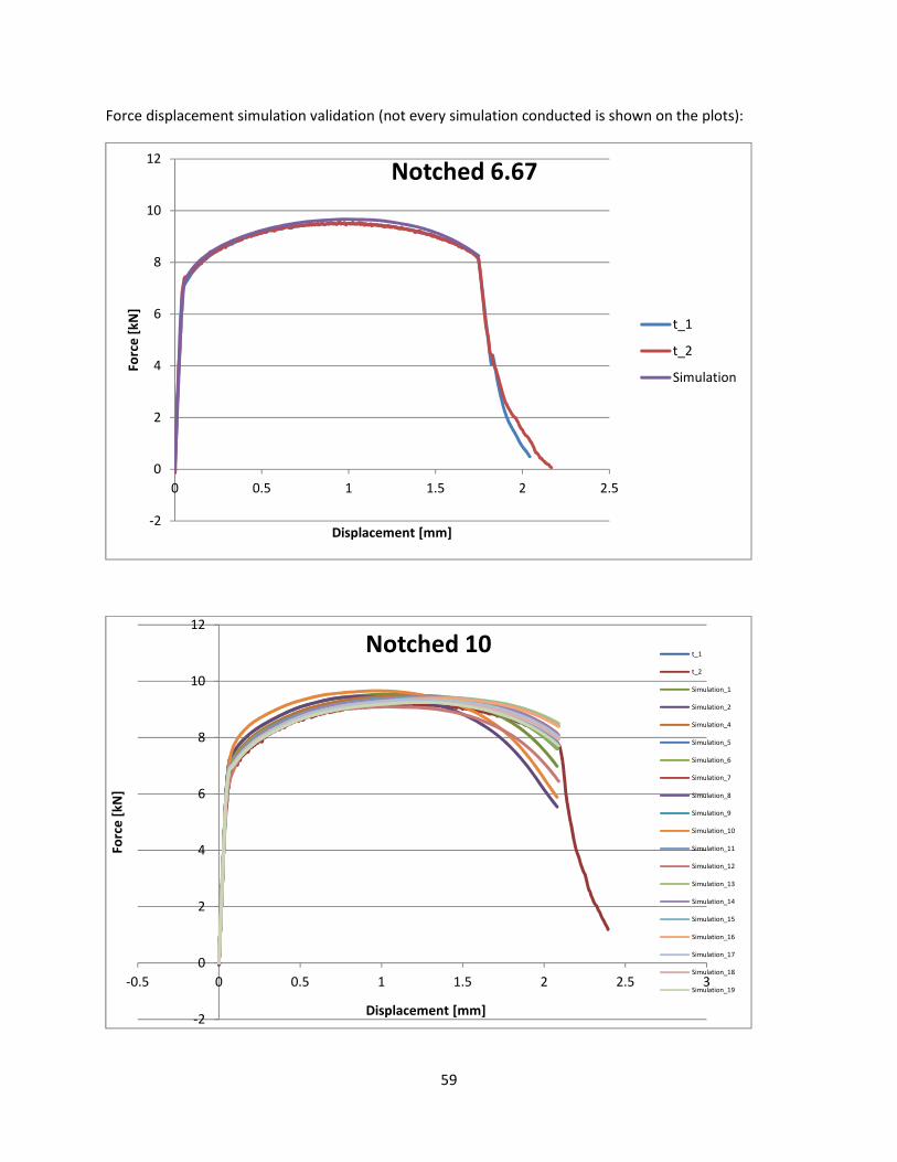
59
Force displacement simulation validation (not every simulation conducted is shown on the plots):
-2
0
2
4
6
8
10
12
0 0.5 1 1.5 2 2.5
Fo
rce
[k
N]
Displacement [mm]
Notched 6.67
t_1
t_2
Simulation
-2
0
2
4
6
8
10
12
-0.5 0 0.5 1 1.5 2 2.5 3
Fo
rce
[k
N]
Displacement [mm]
Notched 10t_1
t_2
Simulation_1
Simulation_2
Simulation_4
Simulation_5
Simulation_6
Simulation_7
Simulation_8
Simulation_9
Simulation_10
Simulation_11
Simulation_12
Simulation_13
Simulation_14
Simulation_15
Simulation_16
Simulation_17
Simulation_18
Simulation_19

60
-2
0
2
4
6
8
10
0 0.5 1 1.5 2 2.5 3 3.5
Fo
rce
[k
N]
Displacement [mm]
Notched 20
t_1
t_2
Simulation 1
Simulation 2
Simulation 3
Simulation 4
Simulation 5
Simulation 6
Simulation 7
Simulation 8
Simulation 9
-2
0
2
4
6
8
10
12
14
0 0.5 1 1.5 2 2.5 3
Fo
rce
[k
N]
Displacement [mm]
Central Hole
t_1
t_2
Simulation
Simulation_2
Simulation_3
Simulation_4
Simulation_5
Simulation_6
Simulation_7
Simulation_8
Simulation_9
Simulation_10

61
-10
0
10
20
30
40
50
60
70
80
90
-5 0 5 10 15 20
Fo
rce
[k
N]
Displacement [mm]
Punch
Test_1
Test_2
3D_DIC_Test1
Simulation
Simulation 2
Simulation 3
Simulation 4
Simulation 6
Simulation 7

62
-10
-5
0
5
10
15
20
25
0 0.1 0.2 0.3 0.4 0.5 0.6 0.7 0.8
Fo
rce
[k
N]
Displacement [mm]
Butterfly Tension
Test
Simulation 1
Simulation 2
Simulation 3
Simulation 4
Simulation 5
-2
0
2
4
6
8
10
12
14
0 1 2 3 4 5 6
Fo
rce
[k
N]
Displacement [mm]
Butterfly Shear
Test_1
Test_2
Simulation