Embed Size (px)
Citation preview
REPORT DOCUMENTATION FORMWAlER RESOURCES RESEARCH CENTER
University of Hawaii at Manoa1 SERIES
NUMBER Technical Report No. 1833TITLE
Groundwater flow and development alternatives:A numerical simulation of Laura, Majuro Atoll,Marshall Islands
8AUfHORS
4REPORTDATE
5NO. OFPAGES
~O.OFTABLES
9GRANT AGENCY
4-B
June 1989
X+ 91
17NO. OF
12 FIGURES 40
John E. GriggsFrank L. Peterson
U.S. Geological SurveyUniversity of Guam
10CONTRACfNUMBER RCUH 3162, RCUH 3292
IlDESCRIPTORS: *groundwater movement, *groundwater potential, *solute transport, simulation analysis,geohydrologyIDENTIFIERS: *groundwater flow, SUTRA, Laura, Majuro Atoll, Marshall Islands
12ABSTRACT (PURPOSE, METIfOD. RESULTS. CONCLUSIONS)
The numerical simulation of groundwater flow with solute transport is described for Laura on MajuroAtoll, Marshall Islands. The primary objective was to investigate strategies for developing and managingthe freshwater resource in Laura. Secondary objectives included performing a sensitivity analysis of theparameters used to calibrate the model and illustrating the effect of density-dependent fluid flow. Thetwo-dimensional mathematical model SUTRA was selected for the simulations because it is based ondensity-dependent fluid flow and solute transportequations. Cartesiancoordinates were used to aproximatea vertical cross section through the Laura area in which three boreholes and three nests of piezometerswere emplaced during another 1987 study. The wells are along a line perpendicular to the ocean andlagoon shorelines running through the central portion of Laura. The model was calibrated in a transientmode with constant sea-level boundary conditions by using observed salinity data. Permeabilities anddispersivities were adjusted during calibration. In a preliminary attempt, tidal boundary conditions werealso used to calibrate the model. Model calibration showed that the 50% isochlordepth depends primarilyon permeability and that the transition wne thickness is most sensitive to transverse dispersivity.Simulated pumping results indicated that gallery-type wells constructed in the center of the islet couldsupply 1.4 to 2.1 million Vday of fresh water. Also, a comparison between flow regimes generated bysingle-phase fluid flow and density-dependent fluid flow demonstrated that the latter greatly affects thegroundwater flow regime and must be included in flow dynamics modeling studies of atolls and smalloceanic islands.
2540 Dole Street· Honolulu, Hawaii 96822· U.S.A.• (808) 956-7847

AlJfHORS:
Dr. John E. GriggsHydrologistHarza Environmental Services150 S. Walker DriveChicago, lllinois 60606Tel.: 312/236-8010
Dr. Frank L. PetersonProfessorDepartment of Geology and GeophysicsUniversity of Hawaii at Manoa2525 Correa RoadHonolulu, Hawaii 96822Tel.: 808/956-7897andResearcherWater Resources Research CenterUniversity of Hawaii at Manoa
The activities on which this report is based were fmanced in part by the Department of theInterior, U.S. Geological Survey, through the Hawaii Water Resources Research Center.
The contents of this publication do not necessarily reflect the views and policies of theDepartment of the Interior, nor does mention of trade names or commercial productsconstitute their endorsement by the United States Government.
GROUNDWATER FLOW AND DEVELOPMENTALTERNATIVES: A Numerical Simulation of Laura,
Majuro Atoll, Marshall Islands
John E. GriggsFrank: L. Peterson
Technical Report No. 183
June 1989
PROJECf COMPLETION REPORTfor
"Atoll Groundwater Systems"Funding Agency: U.S. Geological Survey
Project Nos.: 14-08-0001-G-101314-08-0001-G-1221
Project Periods: 27 June 1985-31 July 19861 August 1986-31 July 1987
Principal Investigator: Frank L. Peterson
and"Atoll Groundwater Development Modeling, Laura Island"
Funding Agency: Water and Energy Research Institute of theWestern Pacific, University of Guam
Project Nos.: RCUH 3162, RCUH 3292Project Periods: 1 June 1986-31 May 1987
1 June 1987-31 May 1988Principal Investigators: Frank L. Peterson
Keith Loague
WATER RESOURCES RESEARCH CENTERUniversity of Hawaii at Manoa
Honolulu, Hawaii 96822

vABSTRACT
The numerical simulation of groundwater flow with solute transpon is described for Laura onMajuro Atoll, Marshall Islands. The primary objective was to investigate strategies fordeveloping and managing the freshwater resource in Laura. Secondary objectives includedperforming a sensitivity analysis of the parameters used to calibrate the model and illustratingthe effect of density-dependent fluid flow. The two-dimensional mathematical model SlITRAwas selected for the simulations because it is based on density-dependent fluid flow and solutetranspon equations.
Canesian coordinates were used to approximate a venical cross section through the Lauraarea in which three boreholes and three nests of piezometers were emplaced during another1987 study. The wells are along a line perpendicular to the ocean and lagoon shorelinesrunning through the central ponion of Laura. The model was calibrated in a transient modewith constant sea-level boundary conditions by using observed salinity data. Permeabilities anddispersivities were adjusted during calibration. In a preliminary attempt, tidal boundaryconditions were also used to calibrate the model.
Model calibration showed that the 50% isochlor depth depends primarily on permeabilityand that the transition zone thickness is most sensitive to transverse dispersivity. Simulatedpumping results indicated that gallery-type wells constructed in the center of the islet couldsupply 1.4 to 2.1 million Vday of fresh water. Also, a comparison between flow regimesgenerated by single-phase fluid flow and density-dependent fluid flow demonstrated that thelatter greatly affects the groundwater flow regime and must be included in flow dynamicsmodeling studies of atolls and small oceanic islands.


vii
CONTENTS
ABSIRACf v
IN1RODUCfION . . . . . . . . . . . . . . . . . . . . . . . . . . . . . . . . . . . . . . . . . . . . . . . . . . . . . . . . . 1
Location and Description ofMajuro Atoll . . . . . . . . . . . . . . . . . . . . . . . . . . . . . . . . . . . . . . 2
Project Scope and Objectives. . . . . . . . . . . . . . . . . . . . . . . . . . . . . . . . . . . . . . . . . . . . . . . 5
MODELING BACKGROUND. . . . . . . . . . . . . . . . . . . . . . . . . . . . . . . . . . . . . . . . . . . . . . . . 5
Modeling of Atolls and Small Oceanic Islands. . . . . . . . . . . . . . . . . . . . . . . . . . . . . . . . . . . 6
MODEL SELECfION AND COMPUTERS. . . . . . . . . . . . . . . . . . . . . . . . . . . . . . . . . . . . . . . 8
SUTRA Model. . . . . . . . . . . . . . . . . . . . . . . . . . . . . . . . . . . . . . . . . . . . . . . . . . . . . . . . . 8
Computers. . . . . . . . . . . . . . . . . . . . . . . . . . . . . . . . . . . . . . . . . . . . . . . . . . . . . . . . . . . . 10
HYDROGEOLOGYOFLAURA 10
Previous Work. . . . . . . . . . . . . . . . . . . . . . . . . . . . . . . . . . . . . . . . . . . . . . . . . . . . . . . . . 10
Near-Surface Hydrogeology. . . . . . . . . . . . . . . . . . . . . . . . . . . . . . . . . . . . . . . . . . . . . . . 12
Additional Field Data 13
MESH DESIGN ANDMODELCALffiRATION 15
Boundary-Value Problem. . . . . . . . . . . . . . . . . . . . . . . . . . . . . . . . . . . . . . . . . . . . . . . . . 15
Mesh Design and Evolution. . . . . . . . . . . . . . . . . . . . . . . . . . . . . . . . . . . . . . . . . . . . . . . . 17
Boundary Conditions . . . . . . . . . . . . . . . . . . . . . . . . . . . . . . . . . . . . . . . . . . . . . . . . . . .. 24
ParaIIleter Estimation 26
Simulations Using Mesh 3 31
Calibration of SUTRA for Laura . . . . . . . . . . . . . . . . . . . . . . . . . . . . . . . . . . . . . . . . . . . . 36
RESULTS............................................................... 43
Sensitivity Analysis . . . . . . . . . . . . . . . . . . . . . . . . . . . . . . . . . . . . . . . . . . . . . . . . . . . .. 44
Validation of Calibrated Model 50
Freshwater Lens Development and Management . . . . . . . . . . . . . . . . . . . . . . . . . . . . . . . . . 51
Influence of Recharge on Pumping 63
Influence of Calibrated ParaIIleters on Lens Creation and Pumping. . . . . . . . . . . . . . . . . . .. 66
Extensions of the Initial Boundary-Value Problem. . . . . . . . . . . . . . . . . . . . . . . . . . . . . . . . 68
Effect of Density-Dependent Fluid Flow. . . . . . . . . . . . . . . . . . . . . . . . . . . . . . . . . . . . . . . 75
Possible Sources of Error . . . . . . . . . . . . . . . . . . . . . . . . . . . . . . . . . . . . . . . . . . . . . . . .. 78
CONCLUSIONS AND FUTURE RESEARCH. . . . . . . . . . . . . . . . . . . . . . . . . . . . . . . . . . . . 84
Technical Conclusions " 85
viii
Managerial Conclusions . . . . . . . . . . . . . . . . . . . . . . . . . . . . . . . . . . . . . . . . . . . . . . . . .. 85
Future Research . . . . . . . . . . . . . . . . . . . . . . . . . . . . . . . . . . . . . . . . . . . . . . . . . . . . . . .. 86
ACKNOWlEOOMENTS . . . . . . . . . . . . . . . . . . . . . . . . . . . . . . . . . . . . . . . . . . . . . . . . . . . . 87
REFERENCES CrrED. . . . . . . . . . . . . . . . . . . . . . . . . . . . . . . . . . . . . . . . . . . . . . . . . . . . . . 88
Figures
I. Schematic Cross Section Showing Island's FreshwaterLens and Transition Zone . . . . . . . . . . . . . . . . . . . . . . . . . . . . . . . . . . . . . . . . . . . . . . . 2
2. Location of Laura, Majuro Atoll, Marshall Islands 3
3. Laura Borehole Sites, Driven Well Sites, andCross-Section Locations Used in lbis Study . . . . . . . . . . . . . . . . . . . . . . . . . . . . . . . . . 4
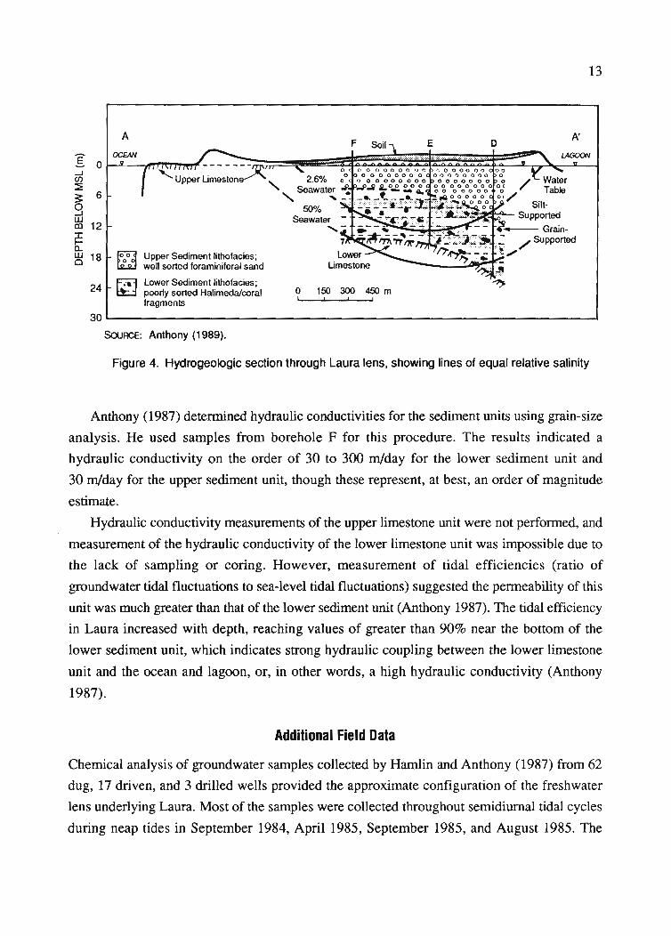
4. Hydrogeologic Section through Laura Lens,Showing Lines of Equal Relative Salinity. . . . . . . . . . . . . . . . . . . . . . . . . . . . . . . . . . . . 13
5. Mesh 3 Hydrogeologic Boundaries andBoundary Conditions for Fluid-Flow Equation. . . . . . . . . . . . . . . . . . . . . . . . . . . . . . . . 19
6. Mesh 4 Boundary Conditions for Fluid-Flow Equation. . . . . . . . . . . . . . . . . . . . . . . . .. 22
7. Mesh 4 Hydrogeologic Boundaries and BoundaryConditions for Fluid-Flow Equation 26
8.1. Unsmoothed Salinity Contours. . . . . . . . . . . . . . . . . . . . . . . . . . . . . . . . . . . . . . . . . .. 33
8.2. Smoothed Salinity Contours. . . . . . . . . . . . . . . . . . . . . . . . . . . . . . . . . . . . . . . . . . . . . 33
9. Salinity Contours in Percentage of Seawater for Simulation M3-TI 35
10. Salinity Contours in Percentage of Seawater forSimulation M3-TI vs. Field Data. . . . . . . . . . . . . . . . . . . . . . . . . . . . . . . . . . . . . . . . . . 35
11. Salinity Contours in Percentage of Seawater forSimulation M3-TI vs. Field Data. . . . . . . . . . . . . . . . . . . . . . . . . . . . . . . . . . . . . . . . . . 37
12. Salinity Contours in Percentage of Seawater forSimulation M4-C4 vs. Field Data . . . . . . . . . . . . . . .. 40
13. Salinity Contours in Percentage of Seawater forSimulation M4-C5 vs. Field Data . . .. 41
14. Hydraulic Conductivity vs. Depth of 50% Isochlor, Wells D, E, and F. . . . . . . . . . . . . .. 48
15. Hydraulic Component of Longitudinal Dispersivity vs.Thickness of Upper Half of Transition Zone, Wells D, E, and F . . . . . . . . . . . . . . . . . .. 48
16. Vertical Component of Longitudinal Dispersivity vs.Thickness of Upper Half of Transition Zone, Wells D, E, and F . . . . . . . . . . . . . . . . . .. 49
17. Transverse Dispersivity vs. Thickness of Upper Half ofTransition Zone, Wells D, E, and F . . . . . . . . . . . . . . . . . . . . . . . . . . . . . . . . . . . . . . .. 50
18. Flow Chart of Ideal Modeling Approach and One Used in This Study 51
19. Laura Area Divided into Series of Representative Slices Thicker Than 1 m . . . . . . . . . . .. 52
20. Salinity Contours in Percentage of Seawater for M4-PI vs. M4-C5 . . . . . . . . . . . . . . . .. 54
21. Salinity Contours in Percentage of Seawater for M4-P4 vs. M4-C5 . . . . . . . . . . . . . . . .. 54
22.
23.
24.
25.
26.
27.
28.
29.
30.
31.
32.
33.
34.
35.1.
35.2.
35.3.
35.4.
36.
37.
38.
39.1.
39.2.
39.3.
39.4.
40.1.
40.2.
40.3.
40.4.
Salinity Contours in Percentage of Seawater for M4-P5 Ys. M4-C5 .
Salinity Contours in Percentage of Seawater for M4-P6 Ys. M4-C5 .
Salinity Contours in Percentage of Seawater for M4-P7 YS. M4-P6 .
Salinity Contours in Percentage of Seawater for MS-Tl YS. M5-Pl .
Curves Integrated to Obtain Quantity of Exploitable Water .
Points Used for Detennining Quantity of Exploitable Water in Laura .
Salinity Contours in Percentage of Seawater for M4-P8 Ys. M4-P7 .
Curves Showing Delay between Changes in the Recharge Rateand Corresponding Change in Depth of 50% Isochlor .
Salinity Contours in Percentage of Seawater for M4-P9 Ys. M4-P7 .
Salinity Contours in Percentage of Seawater for M4-PlO YS. M4-P7 .
Salinity Contours in Percentage of Seawater for M3-Pl YS. M3-TI .
Salinity Contours in Percentage of Seawater for M3-PZ YS. M3-T2 .
Salinity Contours in Percentage of Seawater for M4-El YS. M4-C5 .
Contours Representing 2.6% Isochlor for Initial Conditionsof Simulation M4-E2 .
Contours Representing 2.6% Isochlor after Input of 5 emSeawater oyer One Day for Simulation M4-E2 .
Contours Representing 2.6% Isochlor after Six Months ofFreshwater Recharge for Simulation M4-E2 .
Contours Representing 2.6% Isochlor after 1.5 Years ofFreshwater Recharge for Simulation M4-E2 .
Salinity Contours in Percentage of Seawater for M7-G1 YS. M4-C5 .
Flow Regime for Single-Phase Fluid Flow without Tides .
Flow Regime for Density-Dependent Fluid Flow without Tides .
Flow Regime for Single-Phase Fluid Flow at Mean Rising Tide .
Flow Regime for Single-Phase Fluid Flow at High Tide .
Flow Regime for Single-Phase Fluid Flow at Mean Falling Tide .
Flow Regime for Single-Phase Fluid Flow at Low Tide .
Flow Regime for Density-Dependent Fluid Flow at Mean Rising Tide .
Flow Regime for Density-Dependent Fluid Flow at High Tide .
Flow Regime for Density-Dependent Fluid Flow at Mean Falling Tide .
Flow Regime for Density-Dependent Fluid Flow at Low Tide .
Tables
ix
56
56
57
59
59
61
65
65
67
67
69
69
70
72
72
73
73
76
76
77
79
79
80
80
81
81
82
82
1. Modeling Studies of Small Oceanic Islands and Atolls. . . . . . . . . . . . . . . . . . . . . . . . . . 9
2. Computer Usage 11
3. Well Depth and Salinity Data. . . . . . . . . . . . . . . . . . . . . . . . . . . . . . . . . . . . . . . . . . . . 14

x
4. Mean Monthly Rainfall, 1955-1984, Dalap, Majuro Atoll. . . . . . . . . . . . . . . . . . . . . . . . 15
5. Meshes Used During Calibration . . . . . . . . . . . . . . . . . . . . . . . . . . . . . . . . . . . . . . . . . 18
6. Penneability and Dispersivity Values. . . . . . . . . . . . . . . . . . . . . . . . . . . . . . . . . . . . .. 27
7. Other Parameters . . . . . . . . . . . . . . . . . . . . . . . . . . . . . . . . . . . . . . . . . . . . . . . . . . . . 28
8. Experimental and Calibration Simulations. . . . . . . . . . . . . . . . . . . . . . . . . . . . . . . . . .. 32
9. Meshes after Calibration . . . . . . . . . . . . . . . . . . . . . . . . . . . . . . . . . . . . . . . . . . . . . .. 44
10. Sensitivity-Analysis Simulations. . . . . . . . . . . . . . . . . . . . . . . . . . . . . . . . . . . . . . . .. 44
11. Pumping Simulations . . . . . . . . . . . . . . . . . . . . . . . . . . . . . . . . . . . . . . . . . . . . . . . .. 45
12. Nonpumping Simulations. . . . . . . . . . . . . . . . . . . . . . . . . . . . . . . . . . . . . . . . . . . . .. 46
INTRODUCTION
Atolls commonly fonn rings of small islets composed of intact carbonate reef and reef debris
surrounding a shallow saltwater lagoon. Many of the larger islets contain fresh groundwater in
developable quantities. Freshwater bodies in atolls exist as lenses of fresh water floating on
denser saline water. The density contrast results from the difference in concentration of
dissolved salts in the fluids. The concentration changes from that of fresh water to that of
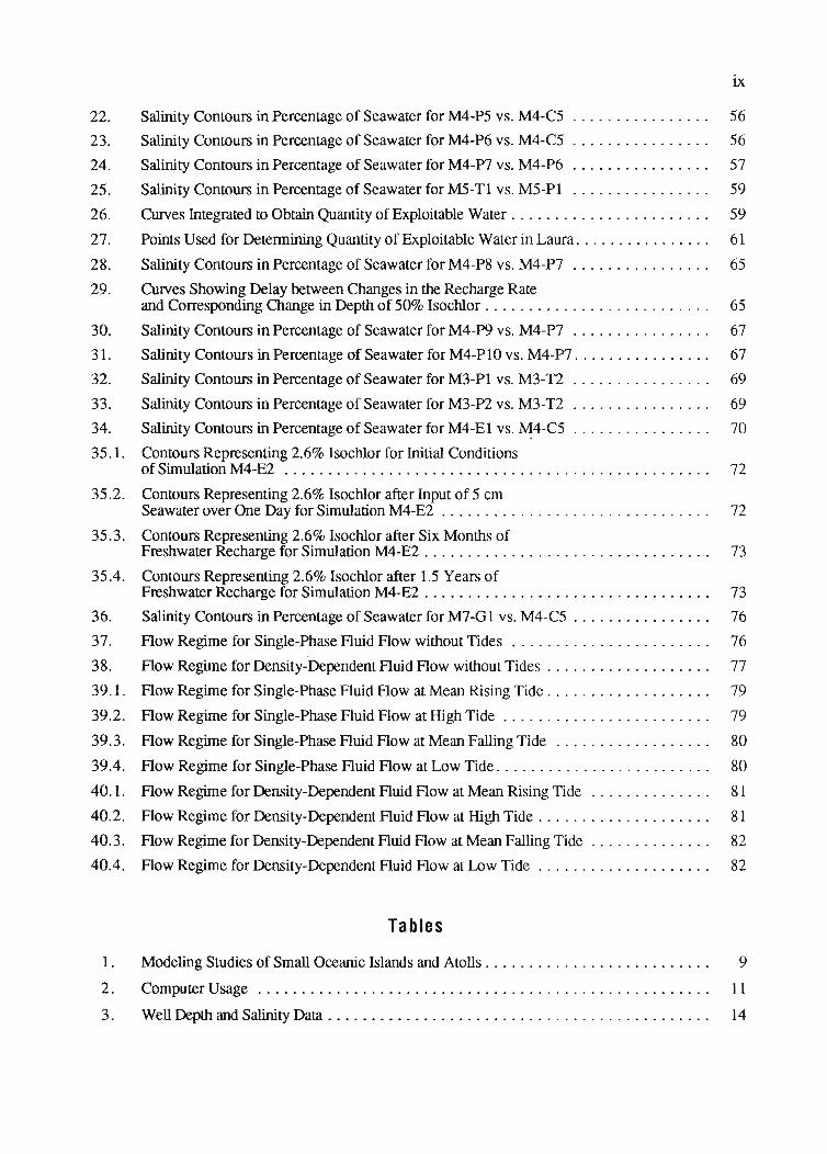
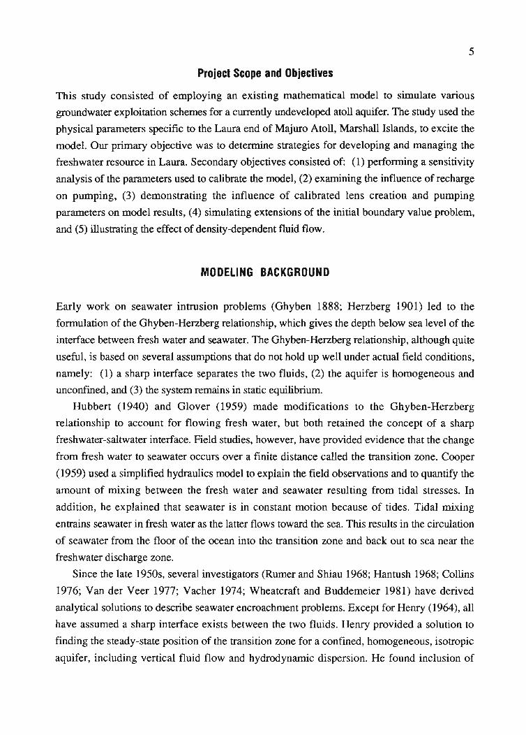
seawater throughout a region tenned the transition zone (Fig. 1).
Under natural conditions, the transition zone typically thickens toward the ocean and
lagoon boundaries and remains in a state of dynamic equilibrium with fresh water flowing
toward the sea above it. Pumping from an aquifer changes the flow regime and increases the
thickness of the transition zone. Consequently, development of potable groundwater resources
in coastal aquifers often leads to degradation of the water quality due to seawater intrusion and
upconing. Poor development schemes or the overpumping of production wells can cause
contamination of the fresh water when the underlying saline water is drawn into wells. Thus,
prior to development of a new groundwater resource, consideration must be given to alternative
modes of exploitation and their probable effects on the groundwater body.
Most hydrogeological studies of small-island aquifers have failed to examine optional
development schemes in detail. Traditional studies have usually included: (1) drilling wells to
delineate the subsurface geology, (2) collecting groundwater samples to determine salinity, (3)
measuring the height of the water table above sea level to estimate the thickness of the
freshwater lens, and (4) calculating the water balance to determine the amount of freshwater
recharge to the aquifer. The interpretation of these data has generally led to the construction of a
geologic cross section with the approximate configuration of the freshwater lens superimposed
on the cross section. Areal maps showing water table elevation and salinity contours have often
accompanied the cross sections. Researchers have used these maps and the water balance
calculations to determine locations to install wells and rates at which to pump the wells. The
objective of many hydrogeological studies of small islands has been to define the sustainable
yield, which represents the maximum amount of potable water that can be continuously
extracted from an aquifer without damaging the resource.
Investigations of the type described here have provided most of the present knowledge of
small island hydraulics. The need for field data requires that traditional investigations continue;
however, time constraints, expense, and potential damage to the resource often preclude
implementation of the various methods of groundwater exploitation in the field. The advent of
high-speed digital computers provides an alternative to typical ways of analyzing the data.
Well-described b0undary value problems can approximate many physical problems of small-
2
ISLANDBOUNDARY
10
I -10zQ
~>W...Jw -30
SEALEVEL
SEAWATER
V' WATER TABLE
FRESHWATER
-50 LI_-'-_-L_--'--_-L-_--'---_-l1_----'-_---'-_---'-_---J1
o 200 400 600 800 1 000
DI5TANCE (m)
SouRCE: Griggs (1989).
Figure 1. Schematic cross section showing island's freshwater lens andtransition zone
island hydraulics. This involves replacing the physical problem with a mathematical equation
and using accepted techniques to solve the equation.
Numerical solution techniques, such as the fmite-difference and finite-element methods
(Remson, Hornberger, and Molz 1971; Pinder and Gray 1977), performed on digital
computers have found widespread acceptance for solving complex hydrogeologic boundary
value problems. Computer simulations have the advantages of speed, versatility,
reproducibility, and cost effectiveness. Mathematical models allow the rapid simulation of
numerous development schemes prior to installation of wells. For this study, we used a
mathematical model to explore various groundwater exploitation schemes for the Laura atoll
aquifer in Majuro Atoll, Marshall Islands.
Location and Description of Majuro Atoll
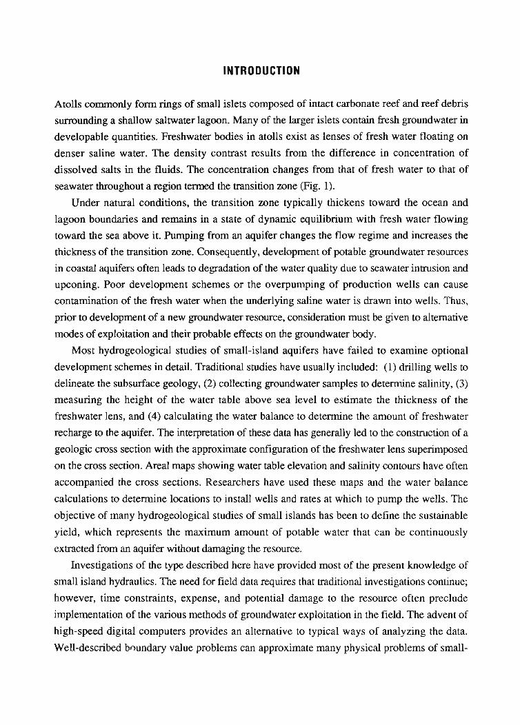
The Marshall Islands are located in the Pacific Ocean approximately 3 600 km southwest of
Hawai'i, and include a wide chain of atolls trending northwest. Majuro Atoll, the capital of the
Republic of the Marshall Islands, lies toward the southeastern end of the chain at latitude 7°N
and longitude 171°E tFig. 2).
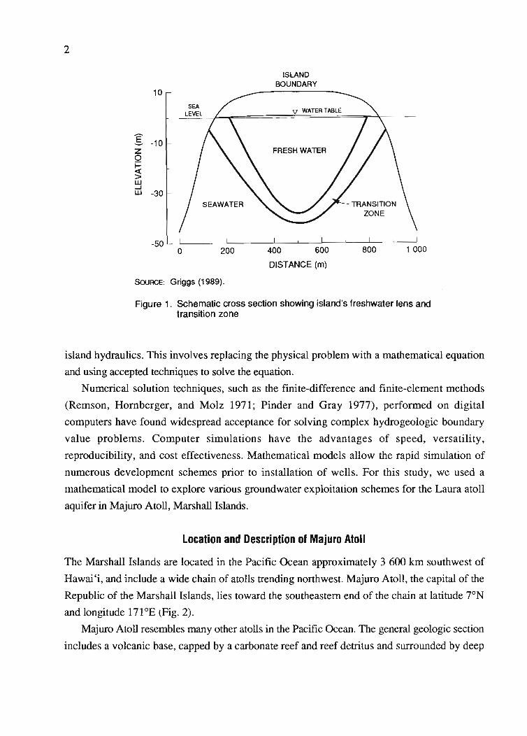
Majuro Atoll resembles many other atolls in the Pacific Ocean. The general geologic section
includes a volcanic base, capped by a carbonate reef and reef detritus and surrounded by deep
3
120°
MAJURO ATOlL
EQUATOR
'. Hawaiian. :·-.Islands
16O"W
• ':'" MAJUROMarshall':<" ATOll
Islands
1600e
. .'
PACIFIC OCEAN
Mariana'Islands:
• Guam
Caroline Islands
<~~"""Australia
120°
Figure 2. Location of Laura, Majuro Atoll, Marshall Islands
ocean. Majuro Atoll is elongated and consists of 64 islets approximately 9 km2 in area,
surrounding a central lagoon of nearly 324 km2. The atoll extends about 40 km from east to
west and 10 km from north to south, and has a maximum elevation of only a few meters above
mean sea level (MSL).
Majuro Atoll has a warm and humid tropical climate. The mean monthly temperature,
nearly constant throughout the year, is 27°C. The average annual rainfall is approximately
3 600 mm (Hamlin and Anthony 1987).
Majuro Island stretches approximately 27 km along the southwestern portion of the atoll
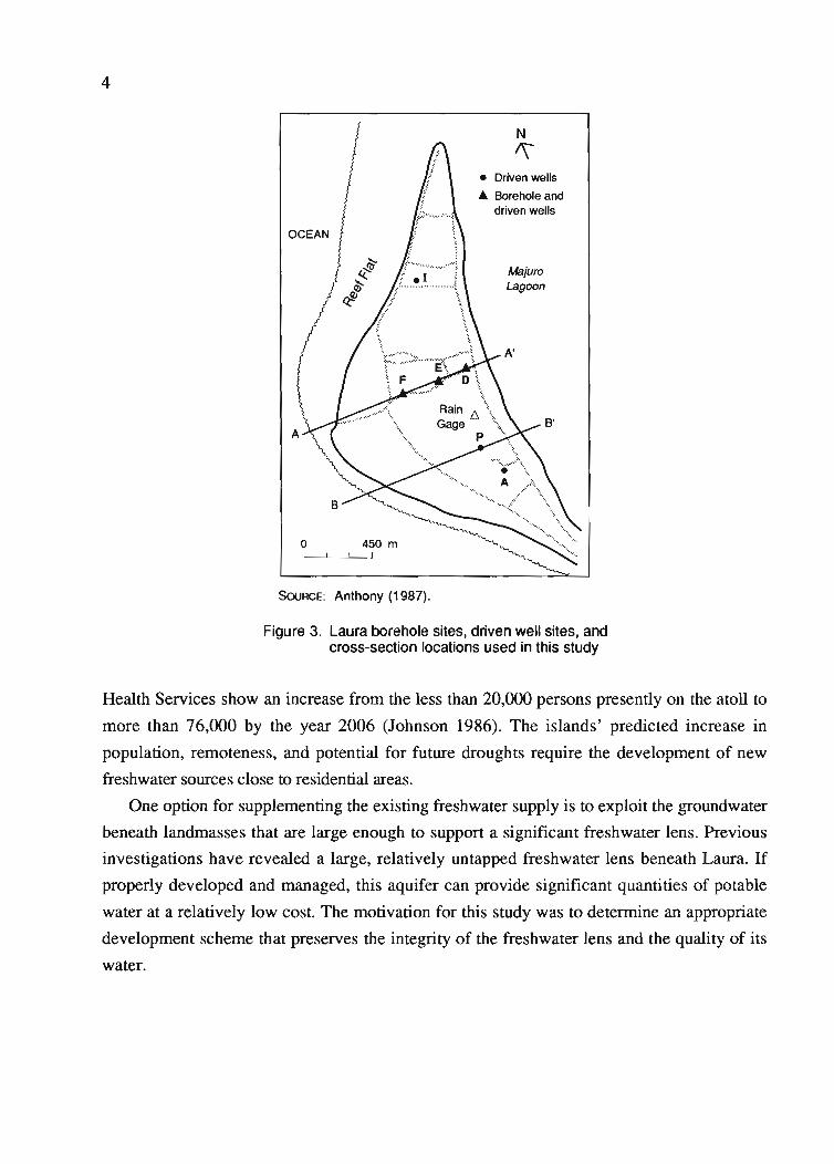
and attains a maximum width of a few hundred meters, except at the westernmost Laura end,
where it is almost 1 km wide at its broadest point (Figs. 2,3). Laura is about 1.8 km2 in area
and supports some 300 homes, in which approximately 800 persons live. Most persons living
on Majuro Atoll reside in the Dalap-Uliga-Darrit area, in the eastern portion of the atoll.
Persons living on Majuro Atoll depend on rain catchment systems and shallow dug wells to
obtain potable water. The combination of population growth and occasional drought is
increasingly stressing existing freshwater supplies. Majuro Atoll's annual population growth
rate of nearly 3.5% is one of the highest in the world. Predictions made by the Marshallese
4
o 450 m
N
1\• Driven wells
A Borehole anddriven wells
MajuroLagoon
SouRCE: Anthony (1987).
Figure 3. Laura borehole sites, driven well sites, andcross-section locations used in this study
Health Services show an increase from the less than 20,000 persons presently on the atoll to
more than 76,000 by the year 2006 (Johnson 1986). The islands' predicted increase in
population, remoteness, and potential for future droughts require the development of new
freshwater sources close to residential areas.
One option for supplementing the existing freshwater supply is to exploit the groundwater
beneath landmasses that are large enough to support a significant freshwater lens. Previous
investigations have revealed a large, relatively untapped freshwater lens beneath Laura. If
properly developed and managed, this aquifer can provide significant quantities of potable
water at a relatively low cost. The motivation for this study was to determine an appropriate
development scheme that preserves the integrity of the freshwater lens and the quality of its
water.
5
Project Scope and Objectives
This study consisted of employing an existing mathematical model to simulate various
groundwater exploitation schemes for a currently undeveloped atoll aquifer. The study used the
physical parameters specific to the Laura end of Majuro Atoll, Marshall Islands, to excite the
model. Our primary objective was to determine strategies for developing and managing the
freshwater resource in Laura. Secondary objectives consisted of: (1) performing a sensitivity
analysis of the parameters used to calibrate the model, (2) examining the influence of recharge
on pumping, (3) demonstrating the influence of calibrated lens creation and pumping
parameters on model results, (4) simulating extensions of the initial boundary value problem,
and (5) illustrating the effect of density-dependent fluid flow.
MODELING BACKGROUND
Early work on seawater intrusion problems (Ghyben 1888; Herzberg 1901) led to the
formulation of the Ghyben-Herzberg relationship, which gives the depth below sea level of the
interface between fresh water and seawater. The Ghyben-Herzberg relationship, although quite
useful, is based on several assumptions that do not hold up well under actual field conditions,
namely: (1) a sharp interface separates the two fluids, (2) the aquifer is homogeneous and
unconfmed, and (3) the system remains in static equilibrium.
Hubbert (1940) and Glover (1959) made modifications to the Ghyben-Herzberg
relationship to account for flowing fresh water, but both retained the concept of a sharp
freshwater-saltwater interface. Field studies, however, have provided evidence that the change
from fresh water to seawater occurs over a finite distance called the transition zone. Cooper
(1959) used a simplified hydraulics model to explain the field observations and to quantify the
amount of mixing between the fresh water and seawater resulting from tidal stresses. In
addition, he explained that seawater is in constant motion because of tides. Tidal mixing
entrains seawater in fresh water as the latter flows toward the sea. This results in the circulation
of seawater from the floor of the ocean into the transition zone and back out to sea near the
freshwater discharge zone.
Since the late 1950s, several investigators (Rumer and Shiau 1968; Hantush 1968; Collins
1976; Van der Veer 1977; Vacher 1974; Wheatcraft and Buddemeier 1981) have derived
analytical solutions to describe seawater encroachment problems. Except for Henry (1964), all
have assumed a sharp interface exists between the two fluids. Henry provided a solution to
finding the steady-state position of the transition zone for a confined, homogeneous, isotropic
aquifer, including vertical fluid flow and hydrodynamic dispersion. He found inclusion of
6
dispersion produced less seawater intrusion and resulted in circulation of the seawater, similar
to the fmdings of Cooper (1959). This particular boundary value problem is well known now
as Henry's problem, and several investigators have used the solution to verify numerical
models.
The advent of high-speed digital computers has led to an increase in the popularity of
numerical solutions to groundwater flow problems. Numerical solutions allow greater
flexibility in the shapes of regions being studied, variation of parameters across the region, and
complexity of boundary conditions. In addition, researchers can simulate transient solutions,
flowing seawater, and velocity-dependent dispersion.
Early pioneering work by Pinder and Cooper (1970) and Reddell and Sunada (1970) used
finite-difference techniques to simulate saltwater intrusion with dispersion. Lee and Cheng
(1974), Segol, Pinder, and Gray (1975), and Segol and Pinder (1976) used finite-element
methods to solve coupled fluid flow and solute transport equations. In recent years, numerical
modeling has become accepted as a valid and versatile tool for studying seawater encroachment
problems, and its use is widespread. However, few modeling investigations have dealt with
atolls and small oceanic islands.
Modeling of Atolls and Small Oceanic Islands
Early modeling of oceanic islands was based on numerous assumptions to limit mathematical
complexity and the computer time necessary for simulations. Fetter (1972) developed a finite
difference model assuming a sharp interface, the Dupuit-Forchheimer approximations, steady
state fluid flow, static seawater, and homogeneous permeabilities. Fetter neglected tides in his
simulations of the South Fork of Long Island in New York. The model produced values for
depths to the interface that were within 6% of field data, although the Dupuit-Forchheimer
approximations failed to allow for a seepage face below sea level at the shoreline. Inclusion of
an outflow face using the solution from Rumer and Shiau (1968) caused the interface to drop
by about 1.5 m.
Lam (1974) used the finite-difference method to calculate the average subsurface
permeability of a radially symmetric atoll. Calibration of the model against tidal efficiency and
phase-lag data for four variations in approximation of the atoll produced permeability values
that ranged over three orders of magnitude. However, the simulations succeeded in
reproducing the gross features of the data. Lam suggested that the simplicity of the
approximations accounted for some of the spread in the calculated permeability values.
Anderson (1976) reported an attempt to simulate groundwater management schemes that
involved two one-dimensional models. The continuously moving interface model included the
7
assumption that the freshwater-saltwater interface moves to an equilibrium position in the sameamount of time as the water table moves to a new equilibrium position. This model displayedlong response times and was unable to reproduce short-term water-level fluctuations.Consequently, Anderson developed a second model, which she called the delayed interfaceresponse (DMI) model. This model introduced a larger error in the materials balance, yet thepredictive simulations employed the DMI model because it could simulate the changes inrecharge patterns observed in field data.
Chidley and Lloyd (1977) studied the lens response to pumping for Grand Cayman Island.They used an effective Ghyben-Herzberg ratio of 1:20 for the base of the potable lens tocalibrate the model. Calibration entailed varying the recharge and permeability spatially to forcethe model results to match field data. Much of the calibration involved reducing the thickness ofthe lens near the edge of the island. Calibrated permeability values ranged over two orders ofmagnitude.
Lloyd et al. (1980), in a study of Tarawa Atoll, demonstrated the effect a drought has on afreshwater lens, though the investigators experienced difficulty in calibrating the model. Thelens appeared too small for high permeabilities, and it rose above land surface for lowpermeabilities. The researchers settled on an intermediate value and assumed that resultsshowing the lens above land surface indicated overland flow.
Falkland (1983) simulated groundwater flow for various lenses of Christmas Island. Hisresults failed to match field data near the edges of the lens because of the Dupuit-Forchheimerapproximations invoked in the model. The lenses became too thick near the edges. In addition,there was numerical instability when he attempted to simulate high pumping rates. He attributedthis to the sharp-interface assumption used in his model.
Ayers and Vacher (1983) developed a simple model to study unsteady flow in thefreshwater lens of Somerset Island, Bermuda. Monthly recharge data for this island wereunknown a priori. Thus, Ayers and Vacher calibrated their model by adjusting the rechargerate. Water table elevations for interior wells compared favorably with observed data, but theresults for wells near the shoreline showed a greater discrepancy. They attributed thediscrepancies to the Dupuit-Forchheimer approximations invoked in the model.
Herman (1984) used the model FEMWAlER to simulate the saturated and unsaturated fluidflow of Enjebi Island, Enewetak Atoll. The model required a single-phase fluid of a constantdensity, which precluded simulation of groundwater management schemes. Herman concludedthat vertical groundwater flow is an important component of atoll flow regimes. This fmdingconflicts with the popular Dupuit-Forchheimer approximations, which include the assumptionthat vertical groundwater movement in freshwater lenses can be neglected.
8
Hogan (1988) employed the fluid-density-dependent solute transport model SUTRA to
simulate groundwater flow for Enjebi Island, Enewetak Atoll. He calibrated permeability using
tidal efficiency and tidal lag data, as did Herman (1984), and obtained permeability values
about six times smaller than Herman's. His calibration of the transport equation involved
assigning a separate dispersivity to each element. The magnitude of each dispersivity value
depended on the path length of the fluid flow through each element, yet Hogan apparently
derived the path length from a solution that neglected density-dependent fluid flow.
Pertinent features of the above-described modeling studies of atolls and small islands are
summarized in Table 1. Of these, only the study by Hogan (1988) used a fluid-density
dependent transport model. That study proceeded concurrently with the one reported here,
although the simulation of pumping schemes was not attempted. Thus, it is believed that the
current research represents the first effort to utilize a fluid-density-dependent mathematical
transport model to simulate groundwater pumping schemes for an atoll.
MODEL SELECTION AND COMPUTERS
Time and budget constraints of this project precluded the time-consuming and expensive task
of developing a model. Therefore, an existing appropriate model was sought. The selection of
a model began with a set of requirements necessary to satisfy the objectives of this study. First,
the model had to solve the coupled transient density-dependent fluid flow and transient solute
transport equations. The flow regime and transport of solute change over time due to recharge
and pumping events. These events eliminated the possibility of using steady-state models, and
the relatively large size of the transition zone in relation to the size of the freshwater nucleus
prohibited the use of sharp-interface models. Second, the model had to be validated.
Demonstration of model accuracy had to include an application of the model to a problem
similar to the one at hand and the production of acceptable results.
SUTRA Model
The model SUTRA (Voss 1984) satisfied the above requirements, though it solves only one
and two-dimensional problems. The search for an accessible three-dimensional fluid-density
dependent model failed. SUIRA can simulate density-dependent fluid flow and solute transport,
though it can accept only one species of solute in any given simulation, and the temperature of
the system must be constant. The transport equation includes equilibrium sorption and both
first-order and zero-order production or decay of the solute. Simulations may involve steady
state or transient boundary conditions, fluid flow, and transport. The model can be used to

TA
BL
E1.
MO
DE
LIN
GST
UD
IES
OF
SMA
LL
OC
EA
NIC
ISL
AN
DS
AN
DA
TO
LL
SN ~
til~
NFL
UID
FLO
W2
~~
°~5
~'U.
lti
lI.l
.l
ffi N~
i~~
Cl
...~"'Cl
E=:
O~
I.l.lN
...c::
~~i
8ce:
j~
AU
TH
OR
c::,<
I)..J
].~
>'''
0§O
ffi~
~~N
I.l.l
en.~=
~~gs
~<~~
Cl
'e§
~~..J~
81;;
~0
<I)
~~~
u~
liiO'
~~
~~~
~>
0::r
:<U
Cl
tIlQ
"
Fette
r(1
972)
IN
NN
NFD
C2/
AN
NN
PN
Lam
(197
4)S
yN
NN
FDR
2NN
NY
TN
And
erso
n(1
976)
IN
YN
NFD
CIN
YN
NH
YC
hidl
ey&
Llo
yd(1
977)
IN
YN
NFD
C2/
Ay
NN
PY
Llo
ydet
aI. (
1980
)I
NY
NN
FDC
2/A
NN
NP
YFa
lkla
nd(1
983)
IN
YN
NFD
C2/
Ay
NN
PY
Aye
rs&
Vac
her
(198
3)I
NY
NN
FDC
2/A
yN
NH
NH
enna
n(1
984)
Sy
yN
NFE
C2N
yN
YT
NH
ogan
(198
7)D
YY
YY
FEC
2Ny
NY
TN
Thi
sSt
udy
DY
YY
YFE
C2N
yN
/YN
/YP
Y11
. int
erfa
ce;
S.si
ngle
-pha
se;
D. d
ensi
ty-d
epen
dent
.2N
. no;
Y. y
es.
3FD
, fin
ite-
diff
eren
ce;
FE, f
mit
e-el
emen
t.4C
, car
tesi
an;
R. r
adia
l.5A
. are
al;
V, v
erti
cal;
1,on
e-di
men
sion
al;
2,tw
o-di
men
sion
al.
6p,
sali
nity
;T
,ti
dal
effi
cien
cy;
H, h
ead.
\0
10
perform unsaturated flow simulations in cross section and saturated flow simulations areally or
in cross section.
This investigation involved the use of SUTRA for which boundary conditions, fluid flow,
and solute transport were transient. The simulated region remained a saturated cross section of
the atoll, and the simulations excluded sorption, production, and decay since chloride is a
conservative ion.
For a more detailed description of capabilities and uses of SUIRA, the reader should consult
Voss (1984).
computers
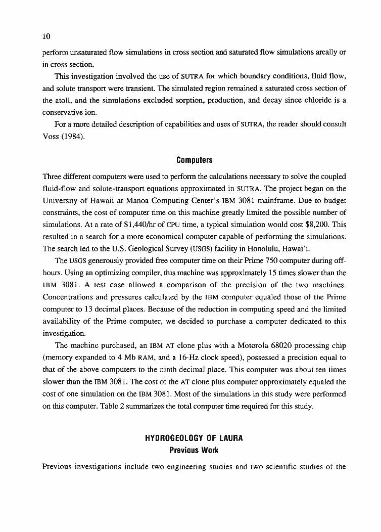
Three different computers were used to perform the calculations necessary to solve the coupled
fluid-flow and solute-transport equations approximated in SUTRA. The project began on the
University of Hawaii at Manoa Computing Center's IBM 3081 mainframe. Due to budget
constraints, the cost of computer time on this machine greatly limited the possible number of
simulations. At a rate of $1,440/hr of CPU time, a typical simulation would cost $8,200. This
resulted in a search for a more economical computer capable of performing the simulations.
The search led to the U.S. Geological Survey (USGS) facility in Honolulu, Hawai'i.
The USGS generously provided free computer time on their Prime 750 computer during off
hours. Using an optimizing compiler, this machine was approximately 15 times slower than the
IBM 3081. A test case allowed a comparison of the precision of the two machines.
Concentrations and pressures calculated by the IBM computer equaled those of the Prime
computer to 13 decimal places. Because of the reduction in computing speed and the limited
availability of the Prime computer, we decided to purchase a computer dedicated to this
investigation.
The machine purchased, an IBM AT clone plus with a Motorola 68020 processing chip
(memory expanded to 4 Mb RAM, and a 16-Hz clock speed), possessed a precision equal to
that of the above computers to the ninth decimal place. This computer was about ten times
slower than the IBM 3081. The cost of the AT clone plus computer approximately equaled the
cost of one simulation on the IBM 3081. Most of the simulations in this study were performed
on this computer. Table 2 summarizes the total computer time required for this study.
HYDROGEOLOGY OF LAURAPrevious Work
Previous investigations include two engineering studies and two scientific studies of the
11
TABLE 2. COMPlITER USAGE
Computer
IBM 3081
Prime 750
AT Clone Plus
CPU Time*(days)
2.25
40
210
Costt
$7,000
$125,000
$660,000
*Equivalent processing times on AT Clone Plus.tEquivalent costs on IBM 3081.
freshwater lens beneath Laura. The fIrst engineering study (Austin, Smith & Associates 1967)proposed the construction of two gallery-type wells in the central portion of the island thatwould supply nearly 600 000 I of fresh water per day. The second study (M&E PacifIc andTenorio & Associates 1979) reiterated the fmdings of Austin, Smith & Associates (1967) andconcentrated on a wastewater facilities plan for the entire atoll.
The fIrst scientifIc study of Laura* focused on water-level and salinity measurements fromshallow dug wells. Huxel produced a contour map of water-table elevations and chlorideconcentrations. He found the freshwater lens to be thicker toward the lagoon side of the isletand estimated a sustainable yield of 730 000 I of fresh water per day per square kilometer oflens area.
The most extensive study of Laura conducted to date (Hamlin and Anthony 1987) consistedof installing 3 drilled wells and 17 driven well points, and performing a geophysical survey.The drilled wells allowed collection of water samples and yielded cores. Clusters of threedriven well points, each at different depths, provided point measurements of salinity andhydraulic head. Salinity measurements from each of the wells established the approximateextent of the freshwater lens, and the cores aided in delineation of the subsurface geology. Thegeophysical survey furnished the position of the geoelectric interface, which represents theboundary between the relatively low electrical conductivity fresh water and the relatively highelectrical conductivity saline water. In addition, Hamlin and Anthony (1987) determined anaverage daily recharge rate to the freshwater lens of 6.93 million 1. From this, they calculated asustainable yield for Laura of approximately 1.5 million Vday of fresh water by assuming thesustainable yield represented roughly 20% of the average daily recharge to the lens and thepotable lens area equaled 1.42 km2. The following sections provide a brief summary of thehydrogeologic results obtained by Hamlin and Anthony (1987).
·C. Huxel (1973): unpublished hydrologic survey data.
12
Near-Surface Hydrogeology
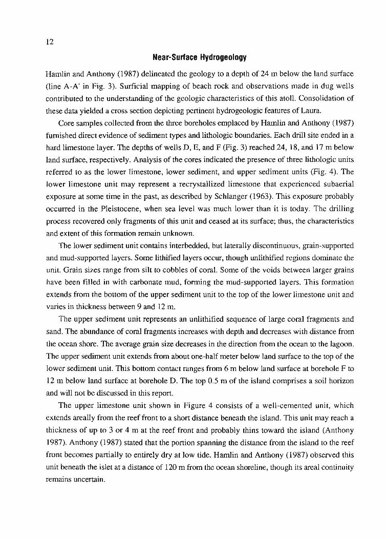
Hamlin and Anthony (1987) delineated the geology to a depth of 24 m below the land surface
(line A-A' in Fig. 3). Surficial mapping of beach rock and observations made in dug wells
contributed to the understanding of the geologic characteristics of this atoll. Consolidation of
these data yielded a cross section depicting pertinent hydrogeologic features of Laura.
Core samples collected from the three boreholes emplaced by Hamlin and Anthony (1987)
furnished direct evidence of sediment types and lithologic boundaries. Each drill site ended in a
hard limestone layer. The depths of wells D, E, and F (Fig. 3) reached 24, 18, and 17 m below
land surface, respectively. Analysis of the cores indicated the presence of three lithologic units
referred to as the lower limestone, lower sediment, and upper sediment units (Fig. 4). The
lower limestone unit may represent a recrystallized limestone that experienced subaerial
exposure at some time in the past, as described by Schlanger (1963). This exposure probably
occurred in the Pleistocene, when sea level was much lower than it is today. The drilling
process recovered only fragments of this unit and ceased at its surface; thus, the characteristics
and extent of this formation remain unknown.
The lower sediment unit contains interbedded, but laterally discontinuous, grain-supported
and mud-supported layers. Some lithified layers occur, though unlithified regions dominate the
unit. Grain sizes range from silt to cobbles of coral. Some of the voids between larger grains
have been filled in with carbonate mud, forming the mud-supported layers. This formation
extends from the bottom of the upper sediment unit to the top of the lower limestone unit and
varies in thickness between 9 and 12 m.
The upper sediment unit represents an unlithified sequence of large coral fragments and
sand. The abundance of coral fragments increases with depth and decreases with distance from
the ocean shore. The average grain size decreases in the direction from the ocean to the lagoon.
The upper sediment unit extends from about one-half meter below land surface to the top of the
lower sediment unit. This bottom contact ranges from 6 m below land surface at borehole F to
12 m below land surface at borehole D. The top 0.5 m of the island comprises a soil horizon
and will not be discussed in this report.
The upper limestone unit shown in Figure 4 consists of a well-cemented unit, which
extends areally from the reef front to a short distance beneath the island. This unit may reach a
thickness of up to 3 or 4 m at the reef front and probably thins toward the island (Anthony
1987). Anthony (1987) stated that the portion spanning the distance from the island to the reef
front becomes partially to entirely dry at low tide. Hamlin and Anthony (1987) observed this
unit beneath the islet at a distance of 120 m from the ocean shoreline, though its areal continuity
remains uncertain.
13
AF A'
Soil E 0
E OCEAN
0-JC/)
::E
~6
UJ12co
F0..UJ 18 ~ Upper Sediment lithofacies;0 well sorted foraminiferal sand
24 ~ Lower Sediment lithofacies;poorly sorted Halimeda/coral 0 150 300 450mfragments
! , , ,
30 "'---------------------------------'
SOURCE: Anthony (1989).
Figure 4. Hydrogeologic section through Laura lens. showing lines of equal relative salinity
Anthony (1987) determined hydraulic conductivities for the sediment units using grain-size
analysis. He used samples from borehole F for this procedure. The results indicated a
hydraulic conductivity on the order of 30 to 300 m/day for the lower sediment unit and
30 m/day for the upper sediment unit, though these represent, at best, an order of magnitude
estimate.
Hydraulic conductivity measurements of the upper limestone unit were not performed, and
measurement of the hydraulic conductivity of the lower limestone unit was impossible due to
the lack of sampling or coring. However, measurement of tidal efficiencies (ratio of
groundwater tidal fluctuations to sea-level tidal fluctuations) suggested the permeability of this
unit was much greater than that of the lower sediment unit (Anthony 1987). The tidal efficiency
in Laura increased with depth, reaching values of greater than 90% near the bottom of the
lower sediment unit, which indicates strong hydraulic coupling between the lower limestone
unit and the ocean and lagoon, or, in other words, a high hydraulic conductivity (Anthony
1987).
Additional Field Data
Chemical analysis of groundwater samples collected by Hamlin and Anthony (1987) from 62
dug, 17 driven, and 3 drilled wells provided the approximate configuration of the freshwater
lens underlying Laura. Most of the samples were collected throughout semidiumal tidal cycles
during neap tides in September 1984, April 1985, September 1985, and August 1985. The
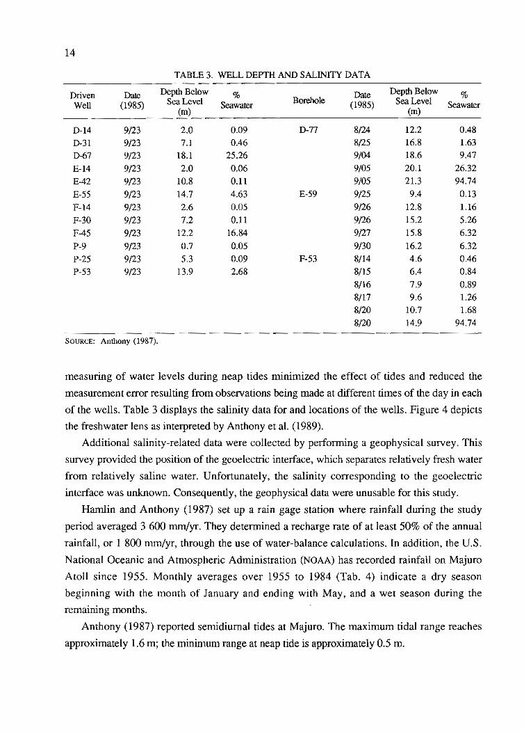
14
TABLE 3. WELL DEPTH AND SALINITY DATA
Driven Date Depth Below % Date Depth Below %Well (1985) SeaLevel Seawater Borehole (1985) SeaLevel Seawater
(m) (m)
D-14 9/23 2.0 0.09 D-77 8/24 12.2 0.48D-31 9/23 7.1 0.46 8/25 16.8 1.63
D-67 9/23 18.1 25.26 9/04 18.6 9.47
E-14 9/23 2.0 0.06 9/05 20.1 26.32
E-42 9/23 10.8 0.11 9/05 21.3 94.74
E-55 9/23 14.7 4.63 E-59 9/25 9.4 0.13
F-14 9/23 2.6 0.05 9/26 12.8 1.16
F-30 9/23 7.2 0.11 9/26 15.2 5.26
F-45 9/23 12.2 16.84 9/27 15.8 6.32
P-9 9/23 0.7 0.05 9/30 16.2 6.32P-25 9/23 5.3 0.09 F-53 8/14 4.6 0.46
P-53 9/23 13.9 2.68 8/15 6.4 0.84
8/16 7.9 0.898/17 9.6 1.26
8/20 10.7 1.68
8/20 14.9 94.74
SOURCE: Anthony (1987).
measuring of water levels during neap tides minimized the effect of tides and reduced the
measurement error resulting from observations being made at different times of the day in each
of the wells. Table 3 displays the salinity data for and locations of the wells. Figure 4 depicts
the freshwater lens as interpreted by Anthony et al. (1989).
Additional salinity-related data were collected by performing a geophysical survey. This
survey provided the position of the geoelectric interface, which separates relatively fresh water
from relatively saline water. Unfortunately, the salinity corresponding to the geoelectric
interface was unknown. Consequently, the geophysical data were unusable for this study.
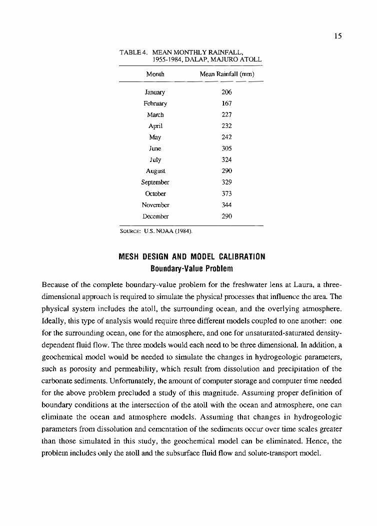
Hamlin and Anthony (1987) set up a rain gage station where rainfall during the study
period averaged 3 600 mrn/yr. They determined a recharge rate of at least 50% of the annual
rainfall, or 1 800 mm/yr, through the use of water-balance calculations. In addition, the U.S.
National Oceanic and Atmospheric Administration (NOAA) has recorded rainfall on Majuro
Atoll since 1955. Monthly averages over 1955 to 1984 (Tab. 4) indicate a dry season
beginning with the month of January and ending with May, and a wet season during the
remaining months.
Anthony (1987) reported semidiumal tides at Majuro. The maximum tidal range reaches
approximately 1.6 m; the minimum range at neap tide is approximately 0.5 m.
15
TABLE 4. MEAN MONTHLY RAINFALL,1955-1984, DALAP, MAJURO ATOLL
Month
January
February
March
April
May
JWle
July
August
September
October
November
December
SOURCE: U.S. NOAA (1984).
Mean Rainfall (mm)
206
167
227
232
242
305
324
290
329
373
344
290
MESH DESIGN AND MODEL CALIBRATIONBoundary-Value Problem
Because of the complete boundary-value problem for the freshwater lens at Laura, a three
dimensional approach is required to simulate the physical processes that influence the area The
physical system includes the atoll, the surrounding ocean, and the overlying atmosphere.
Ideally, this type of analysis would require three different models coupled to one another: one
for the surrounding ocean, one for the atmosphere, and one for unsaturated-saturated density
dependent fluid flow. The three models would each need to be three dimensional. In addition, a
geochemical model would be needed to simulate the changes in hydrogeologic parameters,
such as porosity and permeability, which result from dissolution and precipitation of the
carbonate sediments. Unfortunately, the amount of computer storage and computer time needed
for the above problem precluded a study of this magnitude. Assuming proper definition of
boundary conditions at the intersection of the atoll with the ocean and atmosphere, one can
eliminate the ocean and atmosphere models. Assuming that changes in hydrogeologic
parameters from dissolution and cementation of the sediments occur over time scales greater
than those simulated in this study, the geochemical model can be eliminated. Hence, the
problem includes only the atoll and the subsurface fluid flow and solute-transport model.
16
The use of a three-dimensional subsurface fluid flow and solute-transport model would
have exceeded the resources available for the present study. Time and budget limitations
constrained this investigation to a two-dimensional representation of Laura. Simulation of
density-dependent fluid flow within a freshwater lens necessitated a vertical cross section
instead of an areal region. Assuming that fluid flow near the test boreholes in Laura (see
Fig. 4) is toward the ocean or lagoon, the cross section through these boreholes has two
directions of fluid flow. Under this assumption, no fluid flows into or out of the plane of the
vertical cross section. Two-dimensional fluid flow can be simulated with a two-dimensional
model.
The unsaturated flow portion of the two-dimensional problem requires large amounts of
computer time. According to Freeze and Cherry (1979), the general conclusion of studies that
have included the unsaturated zone is that unsaturated flow above the water table does not
substantially affect the position of the water table during pumpage of unconfined aquifers.
Hence, the approach of this study was to neglect unsaturated fluid flow. The exclusion of
unsaturated fluid flow decreased the execution time needed for this study and increased the
number of possible simulations.
Simplified boundary conditions were used to facilitate the process of identifying when the
simulations reached a steady state. The recharge boundary consisted of a constant recharge
value distributed evenly throughout the year and along the cross section. This was considered
acceptable as a flISt attempt to numerically simulate groundwater flow for Laura because a
variable rate would complicate identification of the steady state. Three simulations included
changes in the recharge rate and its distribution in time (presented in the section on results).
The specified pressure boundaries excluded tides and waves, and MSL for the ocean side of
the islet was set at the same level as for the lagoon side. The exclusion of tides was intended as
a flISt approximation to expedite calibration of the model, with the understanding that the final
calibration would include tidal boundary conditions. However, the inclusion of tides required a
calibration that produced numerically unstable solutions. Thus, tides were ignored for the
development and management simulations. Waves were neglected because the high frequency
of wave impulses would require too small a time-step and thereby limit the number of
simulations. In addition, the erratic nature of waves makes mathematical defmition of the wave
signal extremely complicated. Except for one simulation, which consisted of a higher MSL on
the lagoon side of the islet, the same MSLs on the ocean and lagoon sides of the islet were used
due to the absence of detailed sea-level data on Laura.
17
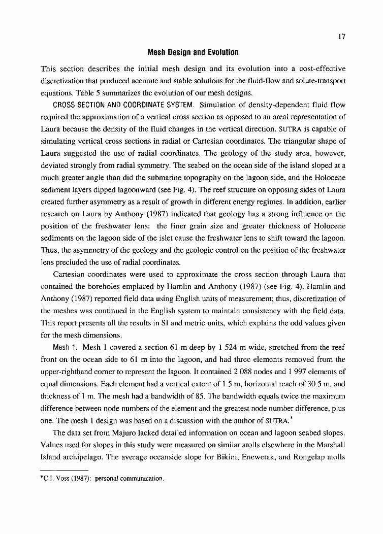
Mesh Design and Evolution
This section describes the initial mesh design and its evolution into a cost-effective
discretization that produced accurate and stable solutions for the fluid-flow and solute-transport
equations. Table 5 summarizes the evolution of our mesh designs.
CROSS SECTION AND COORDINATE SYSTEM. Simulation of density-dependent fluid flow
required the approximation of a vertical cross section as opposed to an areal representation of
Laura because the density of the fluid changes in the vertical direction. SUTRA is capable of
simulating vertical cross sections in radial or Cartesian coordinates. The triangular shape of
Laura suggested the use of radial coordinates. The geology of the study area, however,
deviated strongly from radial symmetry. The seabed on the ocean side of the island sloped at a
much greater angle than did the submarine topography on the lagoon side, and the Holocene
sediment layers dipped lagoonward (see Fig. 4). The reef structure on opposing sides of Laura
created further asymmetry as a result of growth in different energy regimes. In addition, earlier
research on Laura by Anthony (1987) indicated that geology has a strong influence on the
position of the freshwater lens: the finer grain size and greater thickness of Holocene
sediments on the lagoon side of the islet cause the freshwater lens to shift toward the lagoon.
Thus, the asymmetry of the geology and the geologic control on the position of the freshwater
lens precluded the use of radial coordinates.
Cartesian coordinates were used to approximate the cross section through Laura that
contained the boreholes emplaced by Hamlin and Anthony (1987) (see Fig. 4). Hamlin and
Anthony (1987) reported field data using English units of measurement; thus, discretization of
the meshes was continued in the English system to maintain consistency with the field data.
This report presents all the results in SI and metric units, which explains the odd values given
for the mesh dimensions.
Mesh 1. Mesh 1 covered a section 61 m deep by 1 524 m wide, stretched from the reef
front on the ocean side to 61 m into the lagoon, and had three elements removed from the
upper-righthand comer to represent the lagoon. It contained 2 088 nodes and 1 997 elements of
equal dimensions. Each element had a vertical extent of 1.5 m, horizontal reach of 30.5 m, and
thickness of I m. The mesh had a bandwidth of 85. The bandwidth equals twice the maximum
difference between node numbers of the element and the greatest node number difference, plus
one. The mesh I design was based on a discussion with the author of SUTRA.*
The data set from Majuro lacked detailed information on ocean and lagoon seabed slopes.
Values used for slopes in this study were measured on similar atolls elsewhere in the Marshall
Island archipelago. The average oceanside slope for Bikini, Enewetak, and Rongelap atolls
*C.I. Voss (1987): personal communication.

18
TABLE 5. MESHES USED DURING CALIBRATION
No. of No. of CPU Time! Reason forMesh Nodes Elements Bandwidth Time-step Discarding Mesh
(s)
1 2088 1977 85 162 Too expensive
2 841 773 35 3 Unstable; elementsize too large
3 1264 1 167 35 4 Uncertainty ofboundary conditions;element size toolarge
4 1557 1462 51 9 None
SOURCE: Griggs (1989).
Primary Elem. SizeX·Z(m)
30.5 • 1.5
30.5 • 2.0
30.5' 3.0
30.5 • 1.5
equals 35.40, whereas the average lagoon slope to a depth of around 44 m equals 2.30 (Emery,
Tracey, and Ladd 1954). Consequently, approximation of the cross section for mesh 1
included a similar average slope of 2.90 for the lagoon and consisted of truncating the ocean
side at the reef front. The lagoon slope represented a drop of 1.5 m per 30.5 m, or one element
per column. Truncation of the mesh at the reef front was assumed acceptable because it
eliminated only a small submarine portion of the island
Meshes 1 and 2 excluded the portion of the island above MSL, including the portion of the
freshwater lens above MSL. Assuming flow from seepage faces above sea level is negligible,
recharge must pass below sea level before it exits to the ocean. This assumption allowed the
cross-sectional surface to be treated as a recharge boundary and permitted truncation of the
island at sea level.
Approximation of the cross section was based in part on the geologic interpretation of
Hamlin and Anthony (1987) for Laura. Figure 4 depicts the four hydrogeologic units
considered in this study; Figure 5 illustrates the discretization of these formations for mesh 3,
which will be discussed later. The approximation of these four formations for mesh 1 was very
similar to that for mesh 3. Extrapolation of the upper sediment-lower sediment and lower
sediment-lower limestone boundaries to the ocean and lagoon edges of the mesh followed the
boundary trends observed between the boreholes.
Hamlin and Anthony (1987) found the upper limestone below Laura approximately 140 m
inland from the ocean shoreline. Similarly, Ayers and Vacher (1986) located the upper
limestone lying beneath Pingelap Atoll, in the nearby East Caroline Islands, at a distance of up
to a few hundred meters from the ocean shoreline. Thus, using these data and assuming the
observation of Hamlin and Anthony (1987) was not made on the edge of the formation, in
19
It-oI·I--------------IMPERMEABLE-----------.
EIf-oIl.I--------SPECIFIED FLUX--------.j
UPPERW LIMESTONE
OCEAN
IIII-++++++++-H~H-I-t-t++-UPPER SEDIMENT H-+++++++-t+--l--t--1H-
:i!1HI-H-H-++++-H+I-HH-~H-H-++++++-H+I"+IH-H-H-++++++~1I*-++++++-H+-l..-+-1H-I-+-H-++++++++-H-+-l'+-<I-+-l-++-+++++++-H
ffllHl-H-+++++++-t+--l-+-lH-I-+-H-++++++++-H-H..-+-1H-l-+++++~++
cclHl-l-++++++++-t-H--t--1H-H-H-++++++-t-++-t-H-+-1H-H-+++++-+++Q.1II-++++++-+-+-+-l-H~I-+-+-+-++++++--+-++-+-+-lf-+-<~I-+-+++-+-++-+-+-+-+
fil 1HI-H-++++++-H+-l..-+-1H-1-++ LOWER LIMESTONE +-t+-l..-+-1H-I-+-H-+++u:olHl-H-+++++++-t-H--t--1H-H-H-++++++-t-+-+-t-H-+-1H-H-++++++++wQ.Cl)1HI-H-++++++-H+--I-HH-H-H-++++++++-+-t-H-HH-H-++++++++-
o
40
~(/)
:::i:
~ 20~
wCD:r:~0Wo
Io
I400 800 1 200
DISTANCE FROM OCEAN EDGE OF UPPER LIMESTONE (m)
I1 600
SouRCE: Griggs (1989).
Figure 5. Mesh 3 hydrogeologic boundaries and boundary conditions for fluid-flow equation
mesh 1 the upper limestone was extended 213 m into the ocean and 183 m beneath the islet.
Anthony (1987) quoted Buddemeier's estimate of the thickness of the reef plate of no more
than 3.0 to 4.5 m, and Ayers and Vacher (1986) determined that this formation reached a
thickness of 1.7 m near the ocean. Thus, in mesh 1, the upper limestone was assigned a
thickness of 3.0 m.
Testing with mesh 1 proved too expensive. Each time-step required about 162 s of CPU
time on the IBM 3081. Most of the simulations in this study involved a time-step of 0.25 day
for 2 to 3 yr of simulated time. This would have produced an average of 167 hr of CPU time
per simulation. At a rate of $1,440/hr of CPU time on the IBM 3081, each simulation would
have cost approximately $240,000. Thus, budget constraints created the need for a second,
less costly mesh.
Mesh 2. Mesh 2 contained 841 nodes, 773 elements, and a bandwidth of 35. The most
important factor in the length of execution time was the bandwidth of the global matrix, which
contains the summation of integrations over each element. The most efficient scheme for
numbering nodes to minimize the bandwidth consisted of numbering nodes sequentially in the
vertical direction, beginning at the bottom of the mesh. After reaching the top of the mesh in
20
one column of nodes, the next number was assigned to the bottom node of the adjacent
column. The lower-Iefthand-corner node was numbered node 1, and the upper-righthand
corner node was given the largest node number. Reduction of the bandwidth for mesh 2
required reducing the number of nodes in each column.
Modification of the element size for mesh 2 involved changes in the vertical spacing. The
horizontal spacing and mesh thickness remained constant for the entire mesh. Furthermore,
solutions were independent of the mesh thickness because physical parameters and dependent
variables remain constant in the third dimension for two-dimensional models. The vertical
spacing in mesh 2 was twice the spacing for mesh 1 for the portion of the mesh from ground
surface to a 33.5-m depth. Below this depth, the element size was increased by an additional
1.5 m for each element to a maximum of 9.1 m. The bottom of mesh 2 remained 61 m below
the surface of the cross section.
Mesh 2 extended 61 m farther into the lagoon. The fIrst two columns of elements in the
lagoon lacked one element each from the top of the mesh, the third was short two elements,
and the fourth was missing three elements. The region with the removed elements represented
the lagoon. The ocean and islet surface boundaries remained the same as for mesh 1.
SUTRA needs more than one element thickness to represent a hydrogeologic unit.
Permeabilities at nodes along formation edges exhibit a value intermediate between the two
values that meet at the boundary of the units. For example, nodes along the upper limestone
upper sediment boundary in mesh 2 had a permeability intermediate between the two values
assigned to the bordering formations, and nodes along the upper sediment-lower sediment
boundary possessed a permeability intermediate between these two adjoining units. No nodes
on the ocean side of the islet, where only one element thickness represented the upper sediment
and upper limestone units, maintained a permeability equal to the values assigned to these two
formations. Given the coarseness of mesh 2, this result was unavoidable.
Each time-step with mesh 2 used about 3 s of CPU time on the IBM 3081, which
represented a reasonable execution time. Boundary conditions, however, resulted in
instabilities for the mass-transport solution near the lagoon shore. The unstable solution
produced concentrations that oscillated between a range of values. Additional indications of an
unstable solution were concentrations greater than seawater and unrealistic flow regimes. A
stable solution converges on a single value, maintains concentrations equal to or below those of
seawater, and displays a logical flow regime. With mesh 2, the input of freshwater recharge at
one node next to another node held at the concentration of seawater caused the instabilities.
According to Voss (1984), SUTRA needs at least fIve elements across a concentration front to
accurately simulate the physical processes involved in movement of the solute. Mesh 2 violated
this constraint.
21
Mesh 3. Figure 5 illustrates mesh 3, which was used in the first phase of this study. Mesh
3 contained 1 264 nodes and 1 167 elements, and had a bandwidth of 35. Each time-step
required approximately 4 s of CPU time on an IBM 3081. The fmer element size on both edges
of the islet provided a larger number of elements over which the concentration front could be
spread. Each element in the finer areas had a horizontal extent of 7.6 m. The rest of mesh 3
remained the same as mesh 2. The finer discretization on the lagoon side of the atoll stabilized
the mass-transport solution and, although the ocean side did not show any instability, a small
amount of refmement insured a good solution in this part of the mesh as well.
Mesh 4. Mesh 4 was a refmed version of mesh 3. Element sizes were reduced in the same
lens area to provide greater resolution of the transition zone and allow smaller dispersivities.
For numerical stability considerations, the minimum dispersivity value depends on the element
size. The cross section was made deeper and wider to place boundaries farther from the
freshwater lens and to reduce the effects of boundary conditions on the lens. The surface of the
reef plate was lowered in relation to the MSL, and the island dimensions were adjusted to
include the incorporation of a 45° slope on the ocean boundary to more closely approximate
Laura. Mesh 4 had 1 557 nodes, 1 462 elements, and a bandwidth of 51. Each time-step used
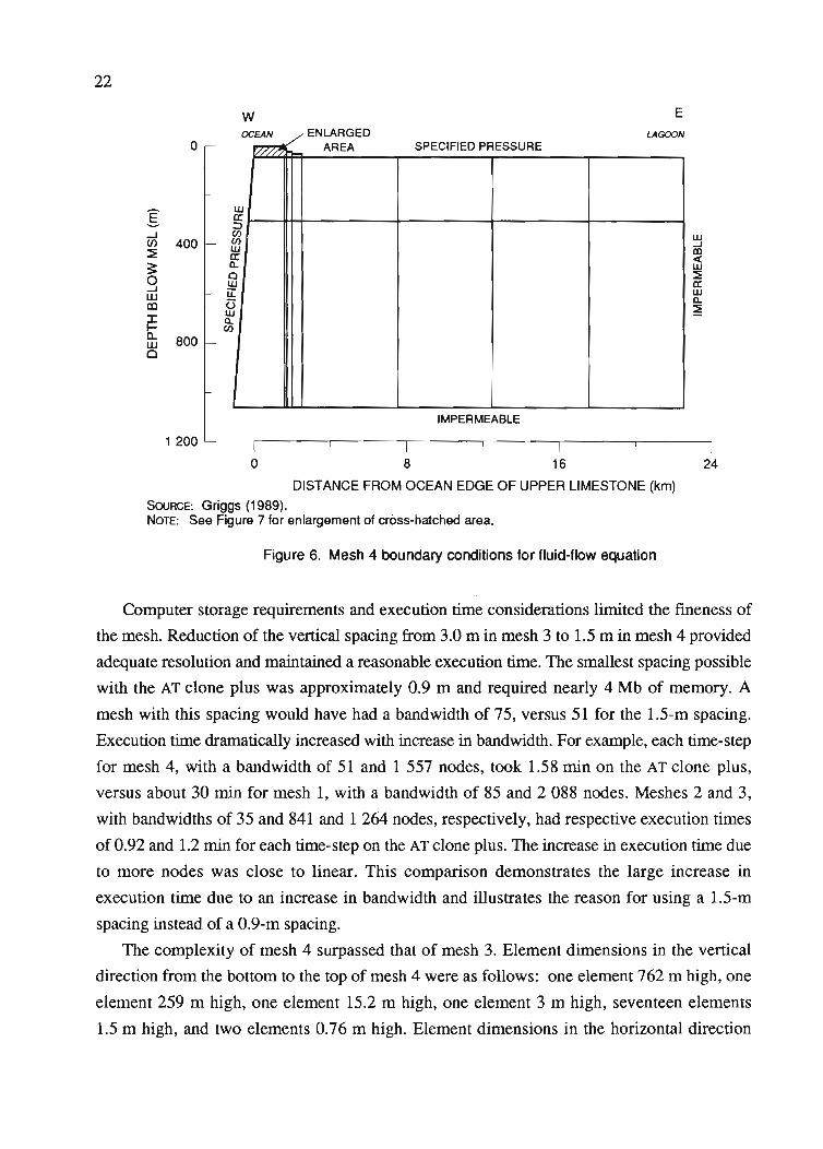
nearly 9 s of CPU time on the IBM 3081. Figure 6 depicts the entire mesh; Figure 7 is an
enlargement of the shaded area, which is roughly equivalent to mesh 3.
The first modification of mesh 3 involved the extension of the bottom boundary from 61 m
to 1 067 m to eliminate the possible influence of the bottom boundary on the freshwater lens.
Based on the findings of Schlanger (1963), it was decided to increase the depth of the cross
section by roughly 1 000 m to obtain a depth to the sediment-basalt interface similar to that
found on Enewetak Atoll. The addition of 5.8 m to this number made it more convenient for
generating data fIles in the English system, so the total increase was 1 006 m. The total depth
of mesh 4 equaled 1 067 m. By way of comparison, two other modeling projects undertaken
on Enjebi Island, Enewetak Atoll (Herman 1984; Hogan 1988), used a depth of 1 277 m,
which represented the depth to the sediment-basalt interface as determined from deep drilling
(Schlanger 1963).
The finer vertical spacing in the lens area of mesh 4 provided greater resolution of
concentration profiles and more control over the thickness of the transition zone because
smaller dispersivities gave stable solutions. If the model spreads a concentration front across
five elements, the smallest transition-zone thickness possible using mesh 3 would be 15.2 m.
According to Anthony (1987), the greatest tnickness of the transition zone in Laura is 7.6 m,
which was so at well D. To simulate this thin transition zone, node spacing had to be 1.5 m or
less.
22
w E
W...Jm<w~a:wll.~
GOOENLARGEDOCEAN LA N
~ AREA SPECIFIED PRESSURE
wIX:::>C/)rnwIX:ll.oWu::(3Wll.rn
o
I...J(/) 400~
~0...JUJCD:r:l-ll. 800UJCl
IMPERMEABLE
I24
Io
1200 I8 16
DISTANCE FROM OCEAN EDGE OF UPPER LIMESTONE (km)
SOURCE: Griggs (1989).NOTE: See Figure 7 for enlargement of cross-hatched area.
Figure 6. Mesh 4 boundary conditions for fluid-flow equation
Computer storage requirements and execution time considerations limited the fineness of
the mesh. Reduction of the vertical spacing from 3.0 m in mesh 3 to 1.5 m in mesh 4 provided
adequate resolution and maintained a reasonable execution time. The smallest spacing possible
with the AT clone plus was approximately 0.9 m and required nearly 4 Mb of memory. A
mesh with this spacing would have had a bandwidth of 75, versus 51 for the 1.5-m spacing.
Execution time dramatically increased with increase in bandwidth. For example, each time-step
for mesh 4, with a bandwidth of 51 and 1 557 nodes, took 1.58 min on the AT clone plus,
versus about 30 min for mesh 1, with a bandwidth of 85 and 2 088 nodes. Meshes 2 and 3,
with bandwidths of 35 and 841 and 1 264 nodes, respectively, had respective execution times
of 0.92 and 1.2 min for each time-step on the AT clone plus. The increase in execution time due
to more nodes was close to linear. This comparison demonstrates the large increase in
execution time due to an increase in bandwidth and illustrates the reason for using a 1.5-m
spacing instead of a 0.9-m spacing.
The complexity of mesh 4 surpassed that of mesh 3. Element dimensions in the vertical
direction from the bottom to the top of mesh 4 were as follows: one element 762 m high, one
element 259 m high, one element 15.2 m high, one element 3 m high, seventeen elements
1.5 m high, and two elements 0.76 m high. Element dimensions in the horizontal direction
23
varied with depth for the four columns of elements closest to the ocean because of the 45°slope. The first five nodes of the bottom row of nodes had a 274-m spacing, and the first fivenodes of the top row a 7.8-m spacing. The remaining nodes in these five columns fell at theintersection of lines drawn from the bottom nodes to the corresponding top nodes and linesdrawn horizontally. The horizontal lines discretized the mesh vertically. The line joining theflith column of nodes stood vertical. The next 38 columns of elements were 30.5 m wide andwere followed by sixteen columns of elements 7.6 m wide, two columns of elements 15.2 mwide, one column of elements 30.5 m wide, three columns of elements 61 m wide, one columnof elements 122 m wide, one column of elements 243.8 m wide, one column of elements609.6 m wide, and four columns of elements 5 km wide.
The fmer discretization beneath the lagoon in mesh 3 proved to be unnecessary because theconcentration of the fluid in this area approached that of seawater. Thus, this region in mesh 4had larger elements than in mesh 3. The finer discretization was needed in areas where theconcentration changed from that of fresh water to seawater. To satisfy this requirement, inmesh 4 the finer element spacing immediately inland of the lagoon extended 61 m farthertoward the ocean than in mesh 3. The extension insured a stable mass-transport solution nearthe lagoon. The large elements at depth and underlying the floor of the lagoon in mesh 4 posedno problems because they contained seawater and were removed from the strong influence ofthe freshwater lens. Voss and Souza (1987) used SUTRA with elements up to 3.75 km in thehorizontal direction and 600 m in the vertical dimension for their simulation of the freshwaterlens beneath the southeast section of the island of O'ahu, Hawai'i. The size of O'ahu'sfreshwater lens greatly exceeded the size of the lens in this study, although the sizes of thesimulated regions were similar.
The extension of mesh 4 to the center of the lagoon served two purposes. First, it placedmuch of the lagoon boundary well away from the region of interest. Errors in approximation ofthis boundary had less influence on the islet the farther away the boundary was. Second,assuming a symmetric atoll, the extension permitted a definition of the center of the lagoon as agroundwater divide.
The maximum depth of the lagoon in mesh 4 was 46 m. The seabed slope from a depth ofo to 30.5 m was 2.9°, decreasing to 1.4° for depths of 30.5 to 46 m. By comparison, theaverage slope to the lagoon floor was 2.2°, which was similar to the findings on Bikini,Enewetak:, and Rongelap atolls. In addition, these three atolls have lagoon-floor slopes of lessthan 0°10' (Emery, Tracey, and Ladd 1954), which allowed the approximation of 0°0' forMajuro Atoll's lagoon-floor slope.
The lowering of the surface of the reef plate to 0.76 m below MSL accommodated theaddition of tidal boundary conditions and conformed to the observations of Anthony (1987)
24
that the reef plate becomes dry to partially dry at low tide. Had a stable calibration with tides
been possible, the reef plate in this study would have become dry at the maximum low tide of
0.76 m below MSL. The nodes along the surface of the reef plate represented specified pressure
nodes. When nodes were assigned a pressure at low tide, specified pressure nodes located at
MSL were a problem: the nodes remained above sea level at low tide, yet this study assumed a
fully saturated simulation region. Elimination of this type of node above the lowest low tide
level obviated this problem for the calibration attempt with tides and for the demonstration of
the effect of density-dependent fluid flow discussed later in this report.
Construction of mesh 4 included the use of information from aerial photographs to refine
the dimensions of the islet. The width of the upper limestone was reduced by 61 m, and the
extension into the ocean beneath the islet was reduced by 30.5 m. The subaerial portion of the
atoll required a shortening of 91.4 m; thus, the total decrease in the width of the islet and reef
plate was 182.9 m. The addition of a 45° slope to the ocean seabed provided a more realistic
approximation of the island, yet maintained the simple mesh design.
Boundary Conditions
Boundary conditions must be defined for both the fluid-flow and mass-transport equations.
Boundary conditions can include specified pressure, specified fluid flux, or impermeable types
for the fluid-flow equation, and specified concentration, specified solute flux, or impermeable
types for the mass-transport equation.
MESH 3. Boundary conditions for mesh 3 (Fig. 5) incorporated flux, constant pressure,
and impermeable types for the fluid-flow equation. The surface of the cross section represented
a flux boundary from the eastern edge of the upper limestone to 61 m from the lagoon. The
upper limestone and 61 m of islet nearest the lagoon were constant pressure boundaries with a
value of 0.0 N/m2. It was assumed that the relatively impermeable nature of the upper
limestone causes rainfall to flow over this unit into the ocean rather than to recharge the
freshwater lens. This situation would prevent development of the portion of the freshwater lens
above MSL and would keep the surface of the upper limestone at atmospheric pressure.
Furthermore, an impermeable boundary failed to accurately describe the portion of the island
nearest the lagoon, and stability considerations discussed in the section on the design of mesh 2
precluded the use of a flux boundary at the lagoon edge of mesh 3. Thus, a constant pressure
boundary appeared to be the most appropriate boundary type for this portion of the mesh.
The ocean and lagoon represented hydrostatic pressure boundaries, with the density of the
fluid equivalent to that of seawater. The initial exclusion of tides simplified identification of a
steady-state freshwater lens. The bottom boundary represented an impermeable base, although
25this certainly is not the case for Majuro Atoll. Hennan (1984) and Hogan (1988) assumed animpenneable boundary at the contact between the Pleistocene limestone and the underlyingvolcanic base for their modeling studies on Enewetak Atoll.
The boundary conditions for the mass-transport equation for mesh 3 depended on theboundary conditions specified for the fluid-flow equation. The approach of this investigationwas to assume the solute did not disperse across boundaries. Hence, mass only advectedacross boundaries with the fluid. Solute was advected across the surface of the cross section,along with the fluid for the flux and constant pressure conditions. Concentrations of theadvected fluid equaled specified values for flux nodes and inflow from pressure nodes, yetequaled the model calculated nodal value for outflow from pressure nodes. Ocean and lagoonboundaries represented constant concentration boundaries with a value of that of seawater. Thebottom boundary represented an impenneable boundary.
MESH 4. Boundary conditions for the fluid-flow equation for mesh 4 remained the same asfor mesh 3 except for a portion of the lagoon boundary and the edges of the islet. Therighthand boundary in Figure 6, the center of the lagoon, represented an impermeableboundary. As explained earlier, the assumption of a symmetric atoll permitted approximation ofthis boundary as a no-flow boundary. Mathematically, a no-flow boundary equals animpermeable boundary.
The flux boundary in mesh 4 extended to within 30.5 m of the fIrst element removed todepict the lagoon (see Fig. 7). This 30.5-m section represented an impenneable boundary forthe following reasons: (1) a flux boundary condition at the edge of the lagoon would havecaused instability, as previously demonstrated with mesh 2, (2) specifIed pressure nodeslocated at MSL were a problem when nodes were assigned a pressure at low tide, as pointed outin the discussion on the lowering of the reef plate for mesh 4, and (3) at high tide, specifIedpressure nodes would have become equivalent to source nodes, possibly producing an unstabletransport solution similar to a flux boundary condition. Consequently, an impenneableboundary appeared to be the only type that would give a stable transport solution with tides.The same boundary condition and reasoning applied to the portion of the upper limestone unitbeneath the islet. Hence, the island portion of the upper limestone was treated as animpermeable boundary, whereas the extension of this unit into the ocean remained a specifIedpressure boundary. It should be noticed that the design of mesh 4 and the assignment ofboundary conditions included considerations for the incorporation of tidal boundaryconditions. Although calibration of the model with tides was not possible with mesh 4, meshfeatures and boundary condition assignments resulting from these considerations were retainedbecause simulation of the effect of density-dependent fluid flow successfully incorporatedtides.
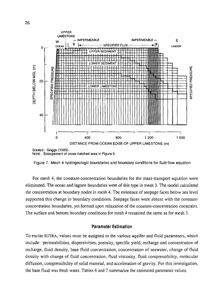
26
UPPERLIMESTONE
o
.s
..Jen::E:: 200..JLUlDJ:.....Q.LUCl
40
wa::::JCI)CI)wa:a..owll:(3wa..CI)
w r IMPERMEABLE IMPERMEABLE~ E
OCEAN I 1-- SPECIFIED FLUX ·1 I LAGOON
UPPER SEDIMENT.• I I I I I I I I I I I
'---LOWER SEDIMENT
LOWER LIMESTONE
wa:::l
~Wa:a..owll:(3wa..CI)
I Io 400 800 1 200
DISTANCE FROM OCEAN EDGE OF UPPER LIMESTONE (m)
SouRCE: Griggs (1989).NOTE: Enlargement of cross-hatched area in Figure 6.
I1 600
Figure 7. Mesh 4 hydrogeologic boundaries and boundary conditions for fluid-flow equation
For mesh 4, the constant-concentration boundaries for the mass-transport equation were
eliminated The ocean and lagoon boundaries were of this type in mesh 3. The model calculated
the concentration at boundary nodes in mesh 4. The existence of seepage faces below sea level
supported this change in boundary conditions. Seepage faces were absent with the constant
concentration boundaries, yet formed upon relaxation of the constant-concentration constraint.
The surface and bottom boundary conditions for mesh 4 remained the same as for mesh 3.
Parameter Estimation
To excite SUTRA, values must be assigned to the various aquifer and fluid parameters, which
include: permeabilities, dispersivities, porosity, specific yield, recharge and concentration of
recharge, fluid density, base fluid concentration, concentration of seawater, change of fluid
density with change of fluid concentration, fluid viscosity, fluid compressibility, molecular
diffusion, compressibility of solid material, and acceleration of gravity. For this investigation,
the base fluid was fresh water. Tables 6 and 7 summarize the estimated parameter values.
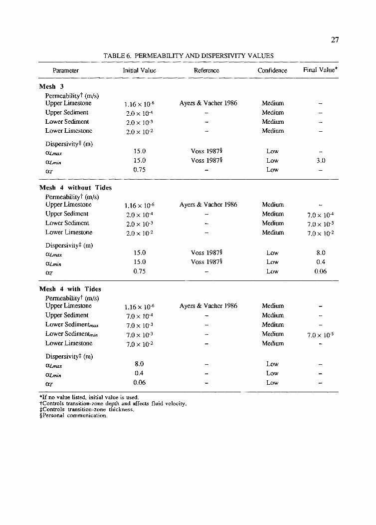
27
TABLE 6. PERMEABILITY AND DISPERSIVITY VALVES
Parameter Initial Value Refereoce Confidence Final Value*
Mesh 3Permeabilityt (m/s)Upper Limestone 1.16 x 10⁻⁶ Ayers & Vacher 1986 MediumUpper Sediment 2.0 x 10⁻⁴ MediumLower Sediment 2.0 x 10⁻³ MediumLower Limestone 2.0 x 10⁻² Medium
Dispersivityt (m)aLmax 15.0 Voss 1987§ LowaLmin 15.0 Voss 1987§ Low 3.0aT 0.75 Low
Mesh 4 without TidesPermeabilityt (m/s)Upper Limestone 1.16 x 10⁻⁶ Ayers & Vacher 1986 MediumUpper Sediment 2.0 x 10⁻⁴ Medium 7.0 x 10⁻⁴Lower Sediment 2.0 x 10⁻³ Medium 7.0 x 10⁻³Lower Limestone 2.0 x 10⁻² Medium 7.0 x 10⁻²
Dispersivityt (m)o.Lmax 15.0 Voss 1987§ Low 8.0aLmin 15.0 Voss 1987§ Low 0.4aT 0.75 Low 0.06
Mesh 4 with TidesPermeabilityt (m/s)Upper Limestone 1.16 x 10⁻⁶ Ayers & Vacher 1986 MediumUpper Sediment 7.0 x 10⁻⁴ MediumLower Sedimentmax 7.0 x 10⁻³ MediumLower Sediment"u,. 7.0 x 10⁻³ Medium 7.0 x 10⁻⁵Lower Limestone 7.0 x 10⁻² Medium
Dispersivityt (m)aLmax 8.0 LowaLmin 0.4 LowaT 0.06 Low
*1£ no value listed, initial value is used.tControls transition-zone depth and affects fluid velocity.:j:Controls transition-zone thickness.§Personal communication.
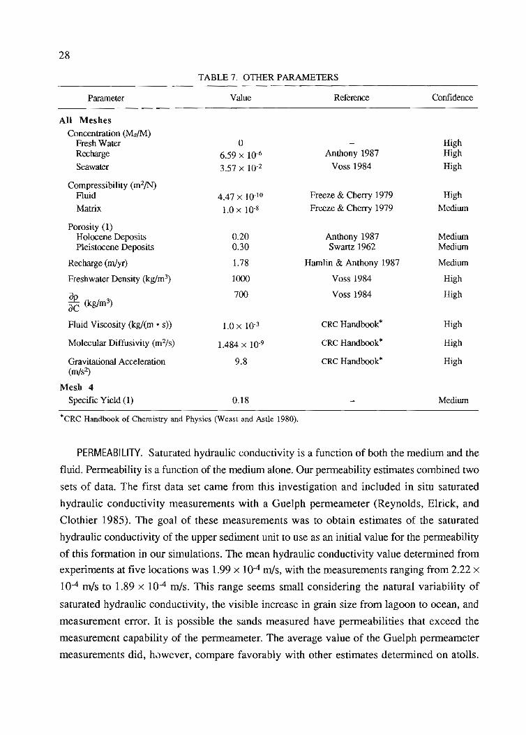
28
TABLE 7. OTHER PARAMETERS
Parameter Value Reference Confidence
All MeshesConcentration (Ms(M)
Fresh Water 0 HighRecharge 6.59 x 10⁻⁶ Anthony 1987 High
Seawater 3.57 x 10⁻² Voss 1984 High
Compressibility (m2/N)Fluid 4.47 x 10⁻¹⁰ Freeze & Cherry 1979 High
Matrix 1.0 x 10⁻⁸ Freeze & Cherry 1979 Mediwn
Porosity (1)Holocene Deposits 0.20 Anthony 1987 MediwnPleistocene Deposits 0.30 Swartz 1962 Mediwn
Recharge (rnjyr) 1.78 Hamlin & Anthony 1987 Mediwn
Freshwater Density (kglm3) 1000 Voss 1984 High
.£e.. (kglm3)700 Voss 1984 High
acFluid Viscosity (kg/(m • s» 1.0 x 10⁻³ CRC Handbook* High
Molecular Diffusivity (m2/s) 1.484 x 10⁻⁹ CRC Handbook* High
Gravitational Acceleration 9.8 CRC Handbook* High(m/sZ)
Mesh 4Specific Yield (1) 0.18 Mediwn
*CRC Handbook of Chemistry and Physics (Weast and Astle 1980).
PERMEABILITY. Saturated hydraulic conductivity is a function of both the medium and the
fluid. Penneability is a function of the medium alone. Our penneability estimates combined two
sets of data. The first data set came from this investigation and included in situ saturated
hydraulic conductivity measurements with a Guelph penneameter (Reynolds, Elrick, and
Clothier 1985). The goal of these measurements was to obtain estimates of the saturated
hydraulic conductivity of the upper sediment unit to use as an initial value for the penneability
of this fonnation in our simulations. The mean hydraulic conductivity value determined from
experiments at five locations was 1.99 x 10⁻⁴ mis, with the measurements ranging from 2.22 x
10-4 mls to 1.89 x 10⁻⁴ mls. This range seems small considering the natural variability of
saturated hydraulic conductivity, the visible increase in grain size from lagoon to ocean, and
measurement error. It is possible the sands measured have penneabilities that exceed the
measurement capability of the penneameter. The average value of the Guelph penneameter
measurements did, h,)wever, compare favorably with other estimates determined on atolls.
29
Anthony (1987) calculated a hydraulic conductivity on the order of 3.53 x 10⁻⁴ m/s for the
upper sediment unit of Laura, using grain-size analysis. From slug tests, Hunt and Peterson
(1980) found a representative value of 1.1 x 10⁻⁴ m/s for the sediments immediately below the
soil horizon on Kwajalein Atoll. Other researchers established hydraulic conductivities for
various islands, including values of 5.2 x 10⁻⁵ m/s for Tarawa Atoll from pump tests (Lloyd et
al. 1980),6.25 x 10-4 m/s for Enewetak Atoll from pump tests (Wheatcraft and Buddemeier
1981), and 2.03 x 10⁻⁵ m/s for Pingelap Atoll from laboratory permeameter measurements
(Ayers and Vacher 1986). Consequently, we felt justified in using the measured value of 2.0 x
10-4 mls for the initial saturated hydraulic conductivity for the upper sediment unit.
The second data set comprised information pertaining to permeability contrast between
hydrogeologic units. Anthony (1987) found the lower sediment unit to be up to one order of
magnitude more permeable than the upper sediment unit in Laura, and he believes, based on
tidal efficiency data, the lower limestone unit is much more permeable than the lower sediment
unit.* The tidal efficiency of the lower limestone approaches 90%, versus roughly 50% for the
lower sediment (Hamlin and Anthony 1987). From pump tests and laboratory permeameter
tests, Hunt and Peterson (1980) derived representative saturated hydraulic conductivities of
1.4 x 10⁻³ mls for sands and gravels and 3.5 x 10⁻³ to 5.3 x 10⁻³ mls for gravels in the lower
part of the aquifer on Kwajalein Atoll; they gave no estimate for the Pleistocene unit.
Wheatcraft and Buddemeier (1981) considered the unconsolidated sediments as a single unit
and estimated that the Pleistocene limestone is substantially more permeable than the overlying
sediments on Enjebi Island, based on tidal efficiency and tidal lag observations. In addition,
two modeling studies of Enewetak Atoll (Herman 1984; Hogan 1988) used a permeability
contrast of two orders of magnitude between the Holocene sediments and the Pleistocene
limestone, based on earlier investigations of Enewetak Atoll and their own calibration results.
Both Herman (1984) and Hogan (1988) treated the Holocene deposits as a single unit.
For this investigation, the permeability used for the lower sediment unit was one order of
magnitude greater than for the upper sediment unit, and the permeability used for the lower
limestone unit was two orders of magnitude larger than for the upper sediment unit (see Figs. 4
and 5). This permeability contrast was employed throughout the calibration of 5UTRA. If the
saturated hydraulic conductivity value of the upper sediment unit was doubled, the
conductivities of the lower sediment and lower limestone units were doubled. This constraint is
reasonable, based on the above-cited studies. The initial saturated hydraulic conductivity values
assigned to the lower sediment and lower limestone units were, respectively, 2.0 x 10⁻³ and
2.0 x 10⁻² mls.
*5.5. Anthony (1987): personal communication.
30
Earlier projects in Laura failed to provide a saturated hydraulic conductivity estimate for the
upper limestone unit, though they determined that it acts as a relatively impermeable formation
because it represents a well-cemented competent rock.* The permeability value used in the
present study came from an investigation of Pingelap Atoll. Ayers and Vacher (1986)
determined that the reef plate on Deke Island, which corresponds to the upper limestone unit of
Laura, has a hydraulic conductivity of approximately 1.16 x 10⁻⁶ mls. The current
investigation employed this value for Laura's upper limestone unit
DISPERSIVITY. No dispersivity values for atolls were found in the literature. The initial
longitudinal dispersivity estimate used in this study was 15 m.* The initial transverse
dispersivity was 1/20 of the longitudinal dispersivity, or 0.75 m.
POROSITY. An effective porosity of 20% for the Holocene sediments, as reported by
Anthony (1987), was used in this study. The effective porosity represents the voids through
which fluid flows, exclusive of isolated or dead-end pores, where water stagnates. Anthony
(1987) obtained the value of 20% from Enos and Sawatsky (1981), who stated that the
effective porosity of Holocene carbonate sediments typically falls in the 10% to 30% range.
The value assigned to the lower limestone unit was 30%. Schlanger (1963) indicated the
Pleistocene limestone may contain large solution features, thereby increasing the original
porosity, and Swartz (1962) measured porosities of greater than 30% for this unit on Enewetak
AtolL The higher porosity for the lower limestone agreed with the value used by Herman
(1984) in his modeling study of Enewetak Atoll.
SPECIFIC YIELD. The modified version of SUrRA, which included the term to account for
storage of water at the water table, required an additional parameter, the specific yield. The
simulations with mesh 4 were done with the modified version, whereas the simulations before
mesh 4 were done with the original version of SUTRA and did not need this parameter. The
field data set lacked information about the specific yield. Therefore, this study estimated the
specific yield to equal 90% of the effective porosity because of the coarseness of the sand.
RECHARGE. The average recharge rates used in this study came from Hamlin and Anthony
(1987), as described previously. The rainfall rate measured by Hamlin and Anthony exceeded
the average rainfall rate measured over the previous 30 years; however, the measurements of
Hamlin and Anthony coincided temporally with the collection of the salinity data used in the
SUTRA calibration. Assuming the lens responds to recharge on a time scale shorter than the
duration of Hamlin and Anthony's study, which was 1.5 yr, the recharge and salinity data
collected by them should have been in a state of quasi-equilibrium. The lens never reaches true
equilibrium because recharge varies continuously in time. In addition, the concentration of
*S.S. Anthony (1987): personal communication.
31
chloride ion in the rainfall was 4 mg/l (Anthony 1987), and this value was used for the
concentration of the recharge in this study.
OTHER PARAMETERS. Many of the remaining parameters needed to excite SUTRA required
specification at a given temperature. Hamlin and Anthony (1987) measured temperatures at
each well sampled on Laura. A representative temperature for groundwater in Laura, based on
their data, is 28°C. However, the density of pure water at approximately 4°C was utilized in
this investigation for the following reason: the simulation of a region with large depth
differences may generate false velocities due to rounded-off errors if the parameter equating the
change in density with change in concentration needs many decimal places to be accurately
represented. The importance of accurately defining this parameter more than offsets the error
introduced by employing the density of pure water at a depressed temperature.* The following
set of parameters alleviated the problem of generating false velocities. The base density of the
fluid was 1 000 kg/m3, and the base concentration was 0.0 MsiM (where M =fluid mass and
M s = solute mass). For a seawater density of 1 024.99 kg/m3 and a concentration of
3.57 x 10⁻² MsiM (Voss 1984), the parameter equating the change in density with change in
concentration was exactly 700 kg/m3.
Other temperature-dependent coefficients and their values included the dynamic viscosity
value of 1.0 x 10⁻³ kg/(m • s) at a temperature of 20°C, fluid compressibility of 4.47 x
10-10 m2/N at a temperature of 30°C, and molecular diffusion of 1.484 x 10⁻⁹ m2/s at 25°C.
These three values were obtained from the CRC Handbook ofChemistry and Physics (Weast
and Astle 1980). The two remaining temperature-independent parameters were the
compressibility of the porous medium and the acceleration due to gravity. Freeze and Cherry
(1979) list an average compressibility for sands of 10-8 m2/N. The CRC Handbook provides a
value of9.8 m/s2 for the acceleration due to gravity.
Simulations Using Mesh 3
The purpose of simulations using mesh 3 was to develop a freshwater lens. A summary of
these simulations is given in Table 8.
The first simulation, M3-TI, furnished the length of time needed to form a freshwater lens
given the set of parameters used as input for the model. This simulation involved the creation
of a freshwater lens, starting from the initial condition of 100% seawater saturating the islet.
The initial pressure field was hydrostatic, with a fluid density equal to that of seawater.
Simulated recharge approximated the average measured recharge rate, distributed evenly in time
and space.
*C.I. Voss (1987): personal communication.
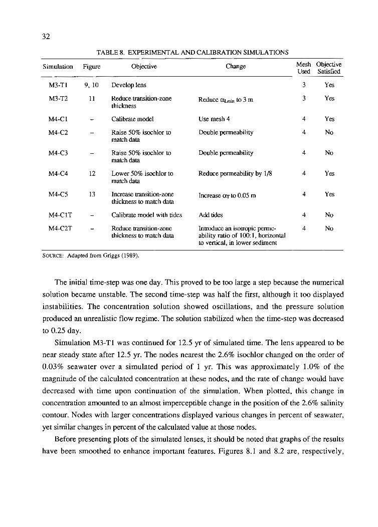
32
TABLE 8. EXPERIMENTAL AND CALIBRAnON SIMULAnONS
Simulation Figure Objective Change Mesh ObjectiveUsed Satisfied
M3-Tl 9,10 Develop lens 3 Yes
M3-T2 11 Reduce transition-zone Reduce 0Lmin to 3 m 3 Yesthickness
M4-CI Calibrate model Use mesh 4 4 Yes
M4-C2 Raise 50% isochlor to Double permeability 4 Nomatch data
M4-C3 Raise 50% isochlor to Double permeability 4 Nomatch data
M4-C4 12 Lower 50% isochlor to Reduce permeability by 1/8 4 Yesmatch data
M4-C5 13 Increase transition-zone Increase aT to 0.05 m 4 Yesthickness to match data
M4-ClT Calibrate model with tides Add tides 4 No
M4-C2T Reduce transition-zone Introduce an isotropic perme- 4 Nothickness to match data ability ratio of 100: 1, horizontal
to vertical, in lower sediment
SOURCE: Adapted from Griggs (1989).
The initial time-step was one day. This proved to be too large a step because the numerical
solution became unstable. The second time-step was half the fIrst, although it too displayed
instabilities. The concentration solution showed oscillations, and the pressure solution
produced an unrealistic flow regime. The solution stabilized when the time-step was decreased
to 0.25 day.
Simulation M3-Tl was continued for 12.5 yr of simulated time. The lens appeared to be
near steady state after 12.5 yr. The nodes nearest the 2.6% isochlor changed on the order of
0.03% seawater over a simulated period of 1 yr. This was approximately 1.0% of the
magnitude of the calculated concentration at these nodes, and the rate of change would have
decreased with time upon continuation of the simulation. When plotted, this change in
concentration amounted to an almost imperceptible change in the position of the 2.6% salinity
contour. Nodes with larger concentrations displayed various changes in percent of seawater,
yet similar changes in percent of the calculated value at those nodes.
Before presenting plots of the simulated lenses, it should be noted that graphs of the results
have been smoothed to enhance important features. Figures 8.1 and 8.2 are, respectively,
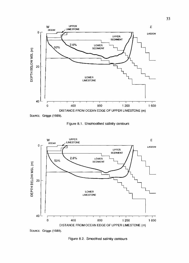
o
I...J(f)
::E3:oi:d 20co::cI0..WCl
40
WOCEAN
LOWERLIMESTONE
E
LAGOON
33
o 400 800 1 200 1 600
DISTANCE FROM OCEAN EDGE OF UPPER LIMESTONE (m)
SouRCE: Griggs (1989).
Figure 8.1. Unsmoothed salinity contours
o
I...J(f)
::E3:oi:d 20co::cI-0..WCl
40
WOCEAN
UPPERLIMESTONE
LOWERLIMESTONE
E
LAGOON
o 400 800 1 200 1 600
DISTANCE FROM OCEAN EDGE OF UPPER LIMESTONE (m)
SouRCE: Griggs (1989).
Figure 8.2. Smoothed salinity contours
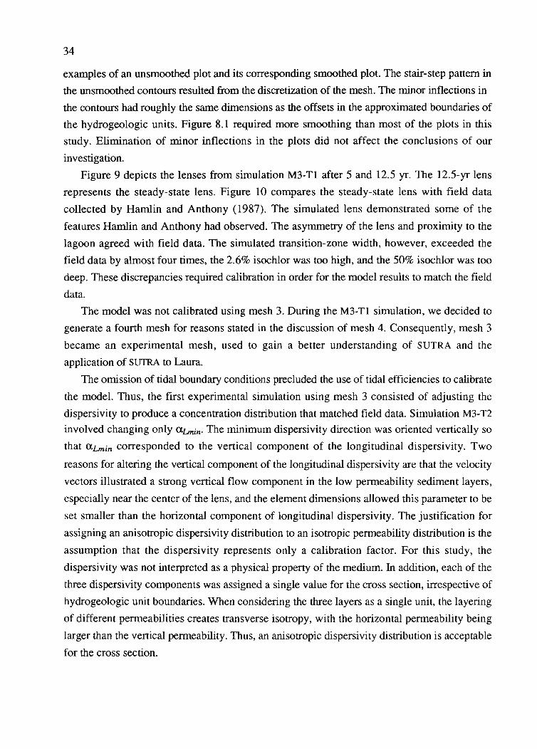
34
examples of an unsmoothed plot and its corresponding smoothed plot. The stair-step pattern in
the unsmoothed contours resulted from the discretization of the mesh. The minor inflections in
the contours had roughly the same dimensions as the offsets in the approximated boundaries of
the hydrogeologic units. Figure 8.1 required more smoothing than most of the plots in this
study. Elimination of minor inflections in the plots did not affect the conclusions of our
investigation.
Figure 9 depicts the lenses from simulation M3-T1 after 5 and 12.5 yr. The 12.5-yr lens
represents the steady-state lens. Figure 10 compares the steady-state lens with field data
collected by Hamlin and Anthony (1987). The simulated lens demonstrated some of the
features Hamlin and Anthony had observed. The asymmetry of the lens and proximity to the
lagoon agreed with field data. The simulated transition-zone width, however, exceeded the
field data by almost four times, the 2.6% isochlor was too high, and the 50% isochlor was too
deep. These discrepancies required calibration in order for the model results to match the field
data.
The model was not calibrated using mesh 3. During the M3-TI simulation, we decided to
generate a fourth mesh for reasons stated in the discussion of mesh 4. Consequently, mesh 3
became an experimental mesh, used to gain a better understanding of SUTRA and the
application of SUTRA to Laura.
The omission of tidal boundary conditions precluded the use of tidal efficiencies to calibrate
the model. Thus, the first experimental simulation using mesh 3 consisted of adjusting the
dispersivity to produce a concentration distribution that matched field data. Simulation M3-T2
involved changing only aLmin' The minimum dispersivity direction was oriented vertically so
that aLmin corresponded to the vertical component of the longitudinal dispersivity. Two
reasons for altering the vertical component of the longitudinal dispersivity are that the velocity
vectors illustrated a strong vertical flow component in the low permeability sediment layers,
especially near the center of the lens, and the element dimensions allowed this parameter to be
set smaller than the horizontal component of longitudinal dispersivity. The justification for
assigning an anisotropic dispersivity distribution to an isotropic permeability distribution is the
assumption that the dispersivity represents only a calibration factor. For this study, the
dispersivity was not interpreted as a physical property of the medium. In addition, each of the
three dispersivity components was assigned a single value for the cross section, irrespective of
hydrogeologic unit boundaries. When considering the three layers as a single unit, the layering
of different permeabilities creates transverse isotropy, with the horizontal permeability being
larger than the vertical permeability. Thus, an anisotropic dispersivity distribution is acceptable
for the cross section.
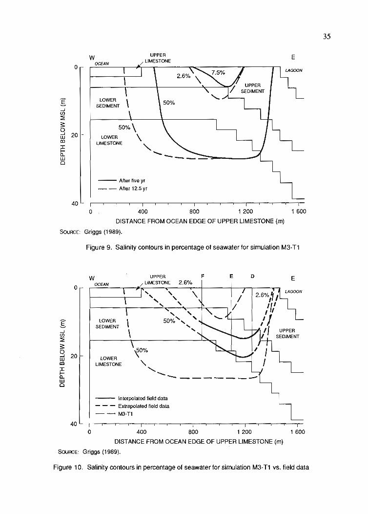
35
LOWERSEDIMENT
LOWERLIMESTONE
o
I....JCf)
:E~
9w 20lDJ:....0..Wo
40
WOCEAN
50%\
\
"- After five yr
- - After 12.5 yr
E
o 400 800 1 200 1 600
DISTANCE FROM OCEAN EDGE OF UPPER LIMESTONE (m)
SouRCE: Griggs (1989).
Figure 9. Salinity contours in percentage of seawater for simulation M3-T1
UPPERSEDIMENT
~O%
".................... .......... _----------
\\
LOWERSEDIMENT
LOWERLIMESTONE
W UPPER F E 0 EOCEAN LIMESTONE 2.6%
0
" \","
I....JCf)
:E~
9 20wlDJ:....0..Wo
- Interpolated field data
- - - Extrapolated field data
- - M3-T1
40 I I
o 400 800 1 200 1 600
DISTANCE FROM OCEAN EDGE OF UPPER LIMESTONE (m)
SouRCE: Griggs (1989).
Figure 10. Salinity contours in percentage of seawater for simulation M3-T1 vs. field data
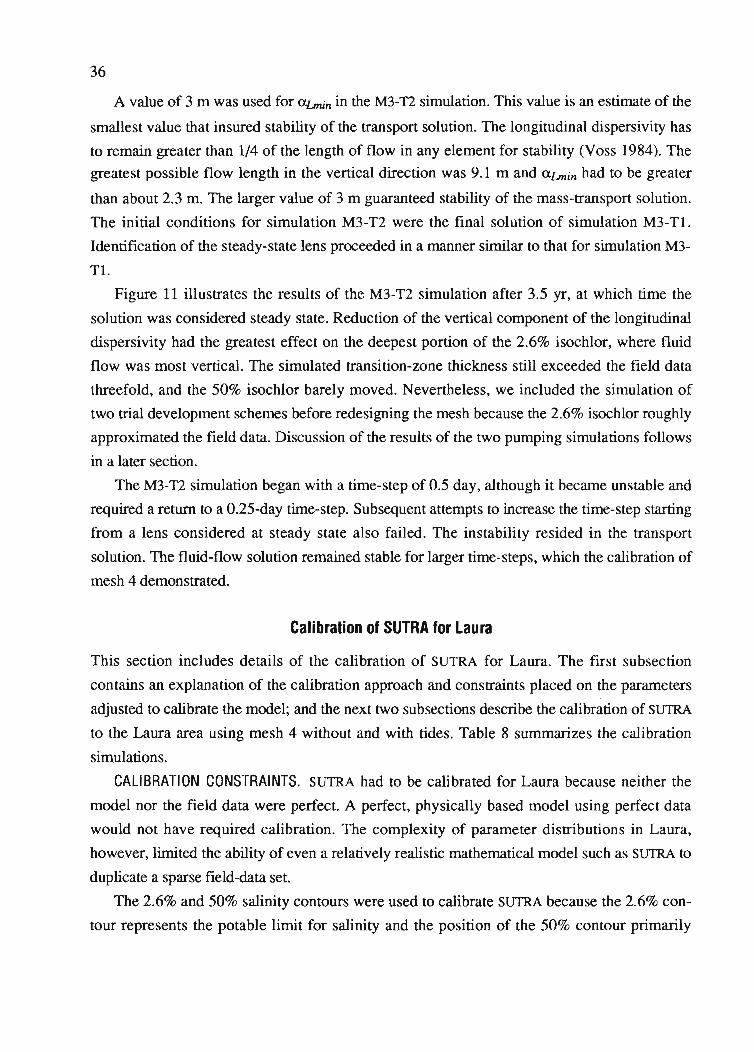
36
A value of 3 m was used for C1.Lmin in the M3-TI simulation. This value is an estimate of the
smallest value that insured stability of the transport solution. The longitudinal dispersivity has
to remain greater than 1/4 of the length of flow in any element for stability (Voss 1984). The
greatest possible flow length in the vertical direction was 9.1 m and (J.Lmin had to be greater
than about 2.3 m. The larger value of 3 m guaranteed stability of the mass-transport solution.
The initial conditions for simulation M3-T2 were the final solution of simulation M3-Tl.
Identification of the steady-state lens proceeded in a manner similar to that for simulation M3
Tl.
Figure 11 illustrates the results of the M3-T2 simulation after 3.5 yr, at which time the
solution was considered steady state. Reduction of the vertical component of the longitudinal
dispersivity had the greatest effect on the deepest portion of the 2.6% isochlor, where fluid
flow was most vertical. The simulated transition-zone thickness still exceeded the field data
threefold, and the 50% isochlor barely moved. Nevertheless, we included the simulation of
two trial development schemes before redesigning the mesh because the 2.6% isochlor roughly
approximated the field data. Discussion of the results of the two pumping simulations follows
in a later section.
The M3-TI simulation began with a time-step of 0.5 day, although it became unstable and
required a return to a 0.25-day time-step. Subsequent attempts to increase the time-step starting
from a lens considered at steady state also failed. The instability resided in the transport
solution. The fluid-flow solution remained stable for larger time-steps, which the calibration of
mesh 4 demonstrated.
Calibration of SUTRA for Laura
This section includes details of the calibration of SUTRA for Laura. The first subsection
contains an explanation of the calibration approach and constraints placed on the parameters
adjusted to calibrate the model; and the next two subsections describe the calibration of SUTRA
to the Laura area using mesh 4 without and with tides. Table 8 summarizes the calibration
simulations.
CALIBRATION CONSTRAINTS. SUTRA had to be calibrated for Laura because neither the
model nor the field data were perfect. A perfect, physically based model using perfect data
would not have required calibration. The complexity of parameter distributions in Laura,
however, limited the ability of even a relatively realistic mathematical model such as SUTRA to
duplicate a sparse field-data set.
The 2.6% and 50% salinity contours were used to calibrate SUTRA because the 2.6% con
tour represents the potable limit for salinity and the position of the 50% contour primarily
37
w F E D E
0OCEAN
~2.6% / I,'" " I '\ " If
50% "g LOWER "-,
SEDIMENT \ "- I ,1 UPPER"--l
\ I SEDIMENTC/)
::E?; \50%0-l 20 \W LOWERCO LIMESTONE "-J:..... "-a.. ""'------------w0
- Interpolated field data
- - - Extrapolated field data
--M3-T2
40 I I Io 400 800 1 200 1 600
DISTANCE FROM OCEAN EDGE OF UPPER LIMESTONE (m)
SouRCE: Griggs (1989).
Figure 11. Salinity contours in percentage of seawater for simulation M3-T2 vs. field data
depended on the permeabilities. This method resulted in determining the position and thickness
of the upper and lower halves of the transition zone using field data from only the upper half.
This is acceptable for two reasons: (1) the majority of the salinity data was collected from the
upper half of the transition zone, and (2) the upper half of the transition zone exerts a greater
influence on the freshwater nucleus because of its proximity.
The approach of the calibration process was to force the model results to match or closely
reproduce field data by adjusting, within their ranges, parameters that gave stable solutions.
The match between simulation results and field data was determined graphically. This
necessitated formulating constraints that defined when a solution became acceptable. The
factors considered to determine constraints included the quantity, quality, and location of the
field data, the possibility of matching all of the field data, the assessment of which field data
were most important, and the effect of matching only the most important field data. Only three
points, estimated from semilog plots of percent seawater versus depth below MSL, defined
each contour. These points provided control over the center of the lens, though they provided
little information about the edges of the lens--especially the ocean edge (see Fig. 10).
Early modeling results indicated the numerical solution could match the field data from
wells D and E with similar parameter sets. A considerably different parameter set, which would
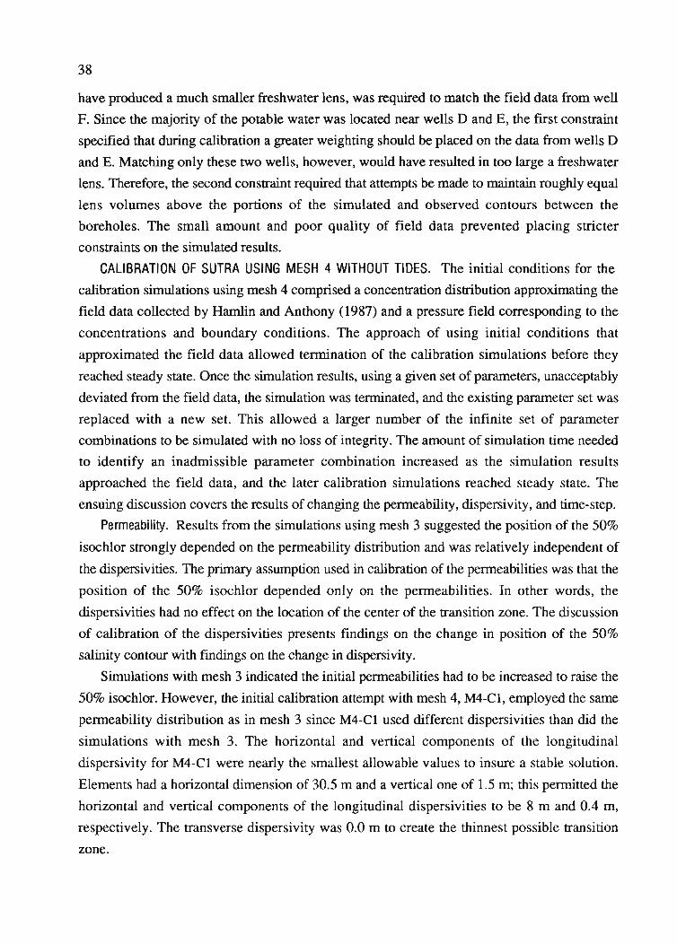
38
have produced a much smaller freshwater lens, was required to match the field data from well
F. Since the majority of the potable water was located near wells D and E, the first constraint
specified that during calibration a greater weighting should be placed on the data from wells D
and E. Matching only these two wells, however, would have resulted in too large a freshwater
lens. Therefore, the second constraint required that attempts be made to maintain roughly equal
lens volumes above the portions of the simulated and observed contours between the
boreholes. The small amount and poor quality of field data prevented placing stricter
constraints on the simulated results.
CALIBRATION OF SUTRA USING MESH 4 WITHOUT TIDES. The initial conditions for the
calibration simulations using mesh 4 comprised a concentration distribution approximating the
field data collected by Hamlin and Anthony (1987) and a pressure field corresponding to the
concentrations and boundary conditions. The approach of using initial conditions that
approximated the field data allowed termination of the calibration simulations before they
reached steady state. Once the simulation results, using a given set of parameters, unacceptably
deviated from the field data, the simulation was terminated, and the existing parameter set was
replaced with a new set. This allowed a larger number of the infinite set of parameter
combinations to be simulated with no loss of integrity. The amount of simulation time needed
to identify an inadmissible parameter combination increased as the simulation results
approached the field data, and the later calibration simulations reached steady state. The
ensuing discussion covers the results of changing the permeability, dispersivity, and time-step.
Permeability. Results from the simulations using mesh 3 suggested the position of the 50%
isochlor strongly depended on the permeability distribution and was relatively independent of
the dispersivities. The primary assumption used in calibration of the permeabilities was that the
position of the 50% isochlor depended only on the permeabilities. In other words, the
dispersivities had no effect on the location of the center of the transition zone. The discussion
of calibration of the dispersivities presents findings on the change in position of the 50%
salinity contour with fmdings on the change in dispersivity.
Simulations with mesh 3 indicated the initial permeabilities had to be increased to raise the
50% isochlor. However, the initial calibration attempt with mesh 4, M4-Cl, employed the same
permeability distribution as in mesh 3 since M4-Cl used different dispersivities than did the
simulations with mesh 3. The horizontal and vertical components of the longitudinal
dispersivity for M4-Cl were nearly the smallest allowable values to insure a stable solution.
Elements had a horizontal dimension of 30.5 m and a vertical one of 1.5 m; this permitted the
horizontal and vertical components of the longitudinal dispersivities to be 8 m and 0.4 m,
respectively. The transverse dispersivity was 0.0 m to create the thinnest possible transition
zone.
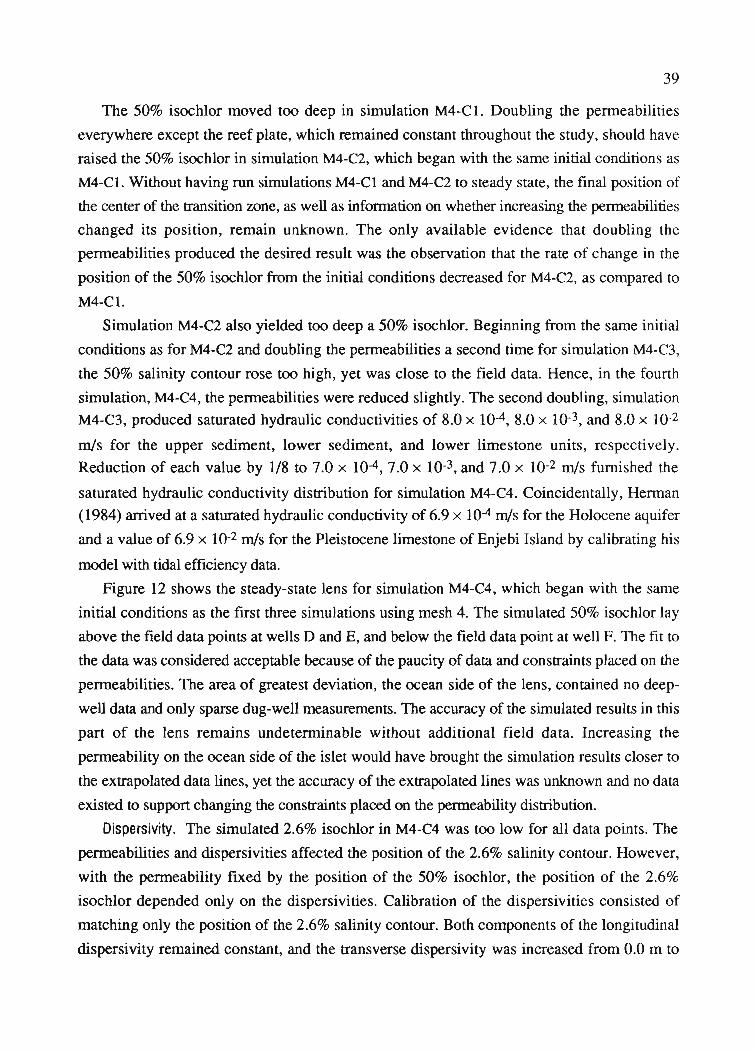
39
The 50% isochlor moved too deep in simulation M4-Cl. Doubling the permeabilitieseverywhere except the reef plate, which remained constant throughout the study, should haveraised the 50% isochlor in simulation M4-C2, which began with the same initial conditions asM4-Cl. Without having run simulations M4-CI and M4-C2 to steady state, the final position ofthe center of the transition zone, as well as information on whether increasing the permeabilitieschanged its position, remain unknown. The only available evidence that doubling thepermeabilities produced the desired result was the observation that the rate of change in theposition of the 50% isochlor from the initial conditions decreased for M4-C2, as compared toM4-Cl.
Simulation M4-C2 also yielded too deep a 50% isochlor. Beginning from the same initialconditions as for M4-C2 and doubling the permeabilities a second time for simulation M4-C3,the 50% salinity contour rose too high, yet was close to the field data. Hence, in the fourthsimulation, M4-C4, the permeabilities were reduced slightly. The second doubling, simulationM4-C3, produced saturated hydraulic conductivities of 8.0 x 10-4,8.0 X 10-3, and 8.0 x 10⁻²
m/s for the upper sediment, lower sediment, and lower limestone units, respectively.Reduction of each value by 1/8 to 7.0 x 10⁻⁴, 7.0 x 10⁻³, and 7.0 x 10⁻² m/s furnished thesaturated hydraulic conductivity distribution for simulation M4-C4. Coincidentally, Herman(1984) arrived at a saturated hydraulic conductivity of 6.9 x 10⁻⁴ m/s for the Holocene aquiferand a value of 6.9 x 10⁻² m/s for the Pleistocene limestone of Enjebi Island by calibrating hismodel with tidal efficiency data.
Figure 12 shows the steady-state lens for simulation M4-C4, which began with the sameinitial conditions as the first three simulations using mesh 4. The simulated 50% isochlor layabove the field data points at wells D and E, and below the field data point at well F. The fit tothe data was considered acceptable because of the paucity of data and constraints placed on thepermeabilities. The area of greatest deviation, the ocean side of the lens, contained no deepwell data and only sparse dug-well measurements. The accuracy of the simulated results in thispart of the lens remains undeterminable without additional field data. Increasing thepermeability on the ocean side of the islet would have brought the simulation results closer tothe extrapolated data lines, yet the accuracy of the extrapolated lines was unknown and no dataexisted to support changing the constraints placed on the permeability distribution.
Oispersivity. The simulated 2.6% isochlor in M4-C4 was too low for all data points. Thepermeabilities and dispersivities affected the position of the 2.6% salinity contour. However,with the permeability fixed by the position of the 50% isochlor, the position of the 2.6%isochlor depended only on the dispersivities. Calibration of the dispersivities consisted ofmatching only the position of the 2.6% salinity contour. Both components of the longitudinaldispersivity remained constant, and the transverse dispersivity was increased from 0.0 m to
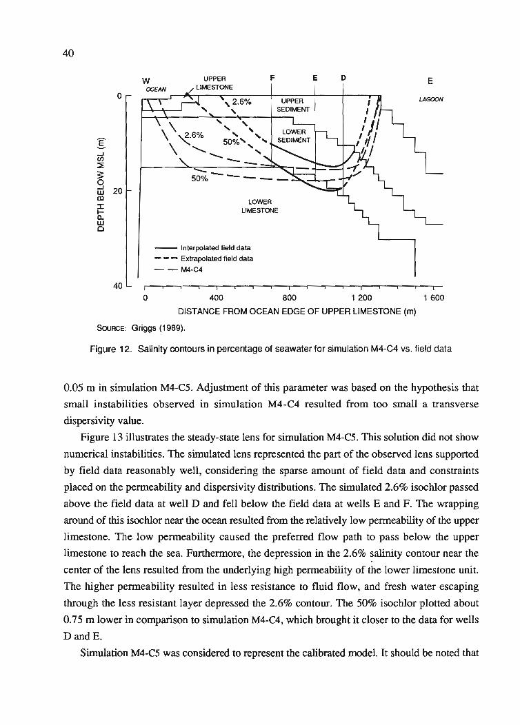
40
o
g...J(/)
~
;::9UJ 20coJ:~0-UJa
40
F
,2.6% UPPER, SEDIMENT
, ,, ,, ,50%' ...
""- '"'- ''--
'--50% -
LOWERLIMESTONE
- Interpolated field data
- - - Extrapolated field data
- - M4-C4
E D E
o 400 800 1 200 1 600
DISTANCE FROM OCEAN EDGE OF UPPER LIMESTONE (m)
SouRCE: Griggs (1989).
Figure 12. salinity contours in percentage of seawater for simulation M4-C4 vs. field data
0.05 m in simulation M4-C5. Adjustment of this parameter was based on the hypothesis that
small instabilities observed in simulation M4-C4 resulted from too small a transverse
dispersivity value.
Figure 13 illustrates the steady-state lens for simulation M4-C5. This solution did not show
numerical instabilities. The simulated lens represented the part of the observed lens supported
by field data reasonably well, considering the sparse amount of field data and constraints
placed on the permeability and dispersivity distributions. The simulated 2.6% isocWor passed
above the field data at well D and fell below the field data at wells E and F. The wrapping
around of this isochlor near the ocean resulted from the relatively low permeability of the upper
limestone. The low permeability caused the preferred flow path to pass below the upper
limestone to reach the sea. Furthermore, the depression in the 2.6% salinity contour near the
center of the lens resulted from the underlying high permeability of the lower limestone unit.
The higher permeability resulted in less resistance to fluid flow, and fresh water escaping
through the less resistant layer depressed the 2.6% contour. The 50% isochlor plotted about
0.75 m lower in comparison to simulation M4-C4, which brought it closer to the data for wells
DandE.
Simulation M4-C5 was considered to represent the calibrated model. It should be noted that
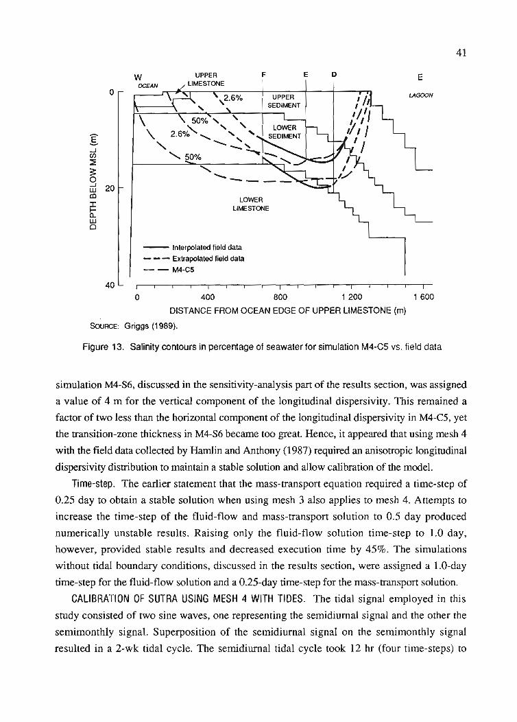
41
EDE
UPPERSEDIMENT
F
LOWERLIMESTONE
\ '" "\ 2.6%.......... "
"-" 50%
WOCEAN
o
I..JC/)
:E3:9w 20alIf-a.wo
- Interpolated field data
- - - Extrapolated field data
-- M4-C5
40o 400 800 1 200 1 600
DISTANCE FROM OCEAN EDGE OF UPPER LIMESTONE (m)
SouRCE: Griggs (1989).
Figure 13. Salinity contours in percentage of seawater for simulation M4-C5 vs. field data
simulation M4-S6, discussed in the sensitivity-analysis part of the results section, was assigned
a value of 4 m for the vertical component of the longitudinal dispersivity. This remained a
factor of two less than the horizontal component of the longitudinal dispersivity in M4-C5, yet
the transition-zone thickness in M4-S6 became too great. Hence, it appeared that using mesh 4
with the field data collected by Hamlin and Anthony (1987) required an anisotropic longitudinal
dispersivity distribution to maintain a stable solution and allow calibration of the model.
Time-step. The earlier statement that the mass-transport equation required a time-step of
0.25 day to obtain a stable solution when using mesh 3 also applies to mesh 4. Attempts to
increase the time-step of the fluid-flow and mass-transport solution to 0.5 day produced
numerically unstable results. Raising only the fluid-flow solution time-step to 1.0 day,
however, provided stable results and decreased execution time by 45%. The simulations
without tidal boundary conditions, discussed in the results section, were assigned a 1.O-day
time-step for the fluid-flow solution and a 0.25-day time-step for the mass-transport solution.
CALIBRATION OF SUTRA USING MESH 4 WITH TIDES. The tidal signal employed in this
study consisted of two sine waves, one representing the semidiurnal signal and the other the
semimonthly signal. Superposition of the semidiurnal signal on the semimonthly signal
resulted in a 2-wk tidal cycle. The semidiurnal tidal cycle took 12 hr (four time-steps) to
42
complete. The time-step for simulations that included tides was 3 hr, with solutions occurring
in the following sequence: MSL, high tide, MSL, and low tide.
Simulation M4-CIT included tidal boundary conditions on the lagoon and ocean
boundaries. The parameter set for this simulation was the calibrated parameter set from M4-C5.
The initial conditions were the final solution of M4-C5. The results of M4-CIT showed that the
potable freshwater nucleus disappeared due to mixing after less than one year of simulated time
and before the solution reached steady state. The freshest water in the simulated region
contained about 10% seawater.
Considering that mixing in SUTRA is simulated with a dispersion model (Voss 1984),
reduction of the mixing required a reduction in the amount of dispersion calculated by the
dispersion model. The two variables that affect dispersion are dispersivity and fluid velocity.
Reducing dispersion by reducing dispersivities would lead to numerical instabilities. Thus, the
only option for reducing the amount of dispersion using mesh 4 was to reduce velocities.
Reduction of fluid velocities required decreasing permeabilities. Observations made during
calibration of SUTRA without tides indicated that the reduction of permeabilities subject to the
initial constraints would have produced too large a lens if the permeabilities were lowered
enough to produce an acceptable thickness of the transition zone. The thickness of the
transition zone appeared to be relatively insensitive to the changes made in the permeabilities.
In fact, the sensitivity analysis demonstrated that a reduction in permeabilities from 7.0 x 10⁻⁴,
7.0 x 10⁻³, and 7.0 x 10⁻² rn/s to 2.0 x 10⁻⁴, 2.0 x 10⁻³, and 2.0 x 10⁻² m/s for, respectively,
the upper sediment, lower sediment, and lower limestone produced a reduction of about 1 m in
the thickness of the upper half of the transition zone and a lens much too large. A reduction of
several meters was required to calibrate SUTRA with tides. Therefore, a new constraint for the
permeability distribution had to be defined.
The new constraint incorporated observations and measurements made by Hamlin and
Anthony (1987). The previous description of the lower sediment unit included the mention of
mud-supported and lithified layers, which were originally ignored because they were
discontinuous and too thin to be approximated with a mesh as coarse as mesh 4. However, the
inability to calibrate the model subject to the original permeability constraints indicated these,
layers might be important in reducing fluid velocities and, thereby, the amount of dispersion.
The new constraint allowed the lower sediment layer to have anisotropic permeability,
although the other three hydrogeologic units retained isotropic permeabilities. According to
Anthony,· the mud-supported layers had permeabilities at least one order of magnitude less
than the upper sediment layer. Therefore, a horizontal-to-vertical permeability ratio of 100:1
·S. Anthony (1987): personal communication.
43was used for the lower sediment layer. This type of anisotropy not only reduced the velocity ofthe fluid in the vertical direction, it also caused fluid flow to be more horizontal, therebyreducing vertical mixing. Permeabilities for simulation M4-C2T were the calibrated values fromM4-C5, except for the vertical component of the lower sediment unit, which was set two ordersof magnitude less than the calibrated horizontal permeability.
Simulation M4-C2T began with initial conditions equal to the final solution of M4-C5. Inputparameters remained the same as for M4-C5, except for the addition of tides and theincorporation of anisotropy in the lower sediment unit. The results of simulation M4-C2T failedto adequately reproduce the field data. After approximately one year of simulated time, thepotable water disappeared due to mixing. The freshest water contained about 4% seawater. Theamount of mixing decreased upon addition of anisotropic permeability, although not enough topursue calibration of SUTRA by adjusting permeabilities. Thus, it was concluded thatcalibration of SUTRA using mesh 4 with tides was not possible for this study.
The inability to calibrate SUlRA with tides using mesh 4 is a limitation of this study. Thislimitation required an additional assumption that the dispersion model employed in SUTRAaccounted for the mixing observed in the field due to tides. The purpose of the dispersionmodel is to account for the lack of information and ability required to simulate the true velocityfield, at least on a microscopic scale. Thus, the above assumption is believed to be acceptable.
It is believed the inability to calibrate SUTRA with tides is a problem of scale related to thecoarseness of mesh 4. As discussed in the section on mesh 4, a fmer discretization was limitedby computer time and computer memory. In addition, the smallest possible element height of0.9 m (see the discussion of mesh 4) would allow a reduction of dispersivity values by lessthan a factor of two. The sensitivity analysis presented in the following section shows thisreduction would not have been large enough to offset the increase of several meters inthickness of the transition zone caused by tides.
RESULTS
This section presents the results of simulations after calibration of SUTRA. Included are: asensitivity analysis for permeability and dispersivity; a discussion of model validation; ananalysis of alternative groundwater development schemes; an analysis of the impact thatchanges in recharge rates have on pumping; a description of the influence that calibratedparameters have on model results; results from several nonpumping simulations; a discussionof the effects of density-dependent fluid flow, both with and without tidal boundary conditions;and a discussion of possible sources of error in the modeling approach. Table 9 outlines

44
TABLE 9. MESHES AFTER CALIBRATION
No. of No. ofCPU Time/ Reason for
Mesh Bandwidth Time-stepNodes Elements (s)
Discarding Mesh
5 1437 1347 51 9 None
6 1 701 1600 51 10 Unstable; element size too
large near grout wall forpermeability contrast used
7 1557 1451 51 9 None
Primary Elem. Size
x·z(m)
30.5· 1.5
30.5 • 1.5
30.5· 1.5
SOURCE: Griggs (1989).
TABLE 10. SENSITIVITY-ANALYSIS SIMULATIONS
Simu-Hydraulic Conductivity (mls) Dispersivity (m)
lationFigure UL US LS LL
x1D-6 x 10-4 x 10-3 x 10⁻² (J./.max aLmin aT
M4-S1 14 1.16 2.00 2.00 2.00 8.0 0.4 0.05
M4-S2 14 1.16 3.50 3.50 3.50 8.0 0.4 0.05
M4-S3 15 1.16 7.00 7.00 7.00 16.0 0.4 0.05
M4-S4 15 1.16 7.00 7.00 7.00 80.0 0.4 0.05
M4-S5 16 1.16 7.00 7.00 7.00 8.0 0.8 0.05
M4-S6 16 1.16 7.00 7.00 7.00 8.0 4.0 0.05
M4-S7 17 1.16 7.00 7.00 7.00 8.0 0.4 0.50
SOURCE: Adapted from Griggs (1989).
NOTE: UL = upper limestone, US = upper sediment, LL = lower limestone, LS = lower sediment
additional meshes, which were generated for the simulations discussed in this section. Table 10
summarizes the sensitivity-analysis simulations. Table 11 lists the pumping simulations.
Table 12 summarizes additional nonpumping simulations.
Sensitivity Analysis
The sensitivity analysis included some of the simulations from calibration of the model, though
most of the sensitivity-analysis simulations followed the calibration phase. The analysis
included only simulations that used mesh 4 and involved adjusting four parameters
independently to obtain information on the sensitivity of the model results to each of those
parameters. This process consisted of varying the permeability, horizontal (maximum)
component of the longitudinal dispersivity, vertical (minimum) component of the longitudinal
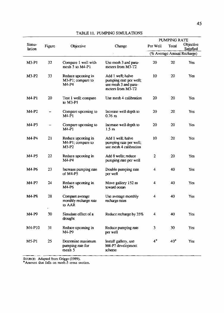
45
TABLE II. PUMPING SIMULAnONS
PUMPING RATESimu- Figure Objective Change Per Well Total ObjectivelationSatisfied
(% Average Annual Recharge)
M3-PI 32 Compare I well with Use mesh 3 and para- 20 20 Yesmesh 3 to M4-PI meters from M3-T2
M3-P2 33 Reduce upconing in Add I well; halve 10 20 YesM3-PI; compare to pumping rate per well;M4-P4 use mesh 3 and para-
meters from M3-T2
M4-PI 20 Test I well; compare Use mesh 4 calibration 20 20 Yesto M3-PI
M4-P2 Compare upconing to Increase well depth to 20 20 YesM4-PI 0.76 m
M4-P3 Compare upconing to Increase well depth to 20 20 YesM4-PI 1.5 m
M4-P4 21 Reduce upconing in Add I well; halve 10 20 YesM4-PI; compare to pumping rate per well;M3-P2 use mesh 4 calibration
M4-P5 22 Reduce upconing in Add 8 wells; reduce 2 20 YesM4-P4 pumping rate per well
M4-P6 23 Increase pwnping rate Double pumping rate 4 40 YesofM4-P5 per well
M4-P7 24 Reduce upconing in Move gallery 152 m 4 40 YesM4-P6 towanl ocean
M4-PS 28 Compare average Use average monthly 4 40 Yesmonthly recharge rate recharge ratestoAAR
M4-P9 30 Simulate effect of a Reduce recharge by 35% 4 40 Yesdrought
M4-PIO 31 Reduce upconing in Reduce pwnping rate 3 30 YesM4-P9 per well
M5-PI 25 Determine maximwn Install gallery. use 4* 40* Yespumping rate for M4-P7 developmentmesh 5 scheme
SOURCE: Adapted from Griggs (1989).*Amount that falls on mesh-5 cross section.
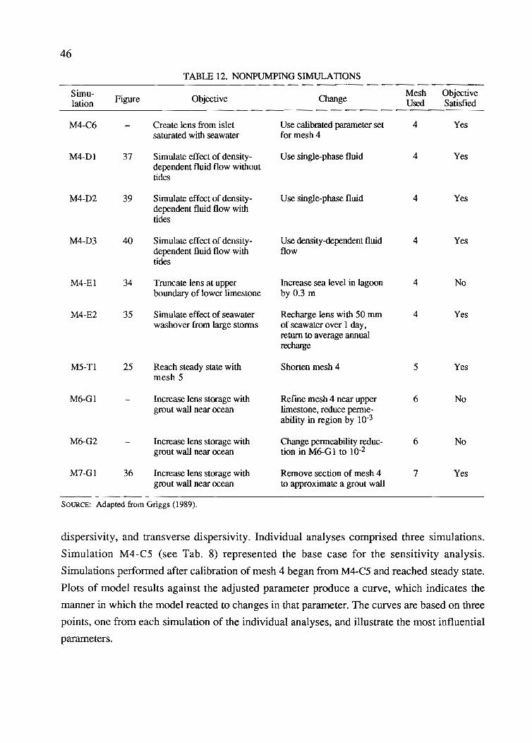
46
TABLE 12. NONPUMPING SIMULATIONS
Simu-Figure Objective Change
Mesh Objectivelation Used Satisfied
M4-C6 Create lens from islet Use calibrated parameter set 4 Yessaturated with seawater for mesh 4
M4-Dl 37 Simulate effect of density- Use single-phase fluid 4 Yesdependent fluid flow withouttides
M4-D2 39 Simulate effect of density- Use single-phase fluid 4 Yesdependent fluid flow withtides
M4-D3 40 Simulate effect of density- Use density-dependent fluid 4 Yesdependent fluid flow with flowtides
M4-El 34 Truncate lens at upper Increase sea level in lagoon 4 Noboundary of lower limestone by 0.3 m
M4-E2 35 Simulate effect of seawater Recharge lens with 50 mm 4 Yeswashover from large storms of seawater over 1 day,
return to average annualrecharge
M5-Tl 25 Reach steady state with Shorten mesh 4 5 Yesmesh 5
M6-Gl Increase lens storage with Refme mesh 4 near upper 6 Nogrout wall near ocean limestone, reduce perme-
ability in region by 10-3
M6-G2 Increase lens storage with Change permeability reduc- 6 Nogrout wall near ocean tion in M6-G 1 to 10-2
M7-Gl 36 Increase lens storage with Remove section of mesh 4 7 Yesgrout wall near ocean to approximate a grout wall
SOURCE: Adapted from Griggs (1989).
dispersivity, and transverse dispersivity. Individual analyses comprised three simulations.
Simulation M4-C5 (see Tab. 8) represented the base case for the sensitivity analysis.
Simulations performed after calibration of mesh 4 began from M4-C5 and reached steady state.
Plots of model results against the adjusted parameter produce a curve, which indicates the
manner in which the model reacted to changes in that parameter. The curves are based on three
points, one from each simulation of the individual analyses, and illustrate the most influential
parameters.
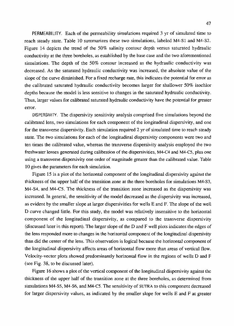
47
PERMEABILITY. Each of the permeability simulations required 3 yr of simulated time to
reach steady state. Table 10 summarizes these two simulations, labeled M4-S1 and M4-S2.
Figure 14 depicts the trend of the 50% salinity contour depth versus saturated hydraulic
conductivity at the three boreholes, as established by the base case and the two aforementioned
simulations. The depth of the 50% contour increased as the hydraulic conductivity was
decreased. As the saturated hydraulic conductivity was increased, the absolute value of the
slope of the curve diminished. For a fIxed recharge rate, this indicates the potential for error as
the calibrated saturated hydraulic conductivity becomes larger for shallower 50% isochlor
depths because the model is less sensitive to changes in the saturated hydraulic conductivity.
Thus, larger values for calibrated saturated hydraulic conductivity have the potential for greater
error.
DISPERSIVITY. The dispersivity sensitivity analysis comprised fIve simulations beyond the
calibrated lens, two simulations for each component of the longitudinal dispersivity, and one
for the transverse dispersivity. Each simulation required 2 yr of simulated time to reach steady
state. The two simulations for each of the longitudinal dispersivity components were two and
ten times the calibrated value, whereas the transverse dispersivity analysis employed the two
freshwater lenses generated during calibration of the dispersivities, M4-C4 and M4-C5, plus one
using a transverse dispersivity one order of magnitude greater than the calibrated value. Table
10 gives the parameters for each simulation.
Figure 15 is a plot of the horizontal component of the longitudinal dispersivity against the
thickness of the upper half of the transition zone at the three boreholes for simulations M4-S3,
M4-S4, and M4-C5. The thickness of the transition zone increased as the dispersivity was
increased. In general, the sensitivity of the model decreased as the dispersivity was increased,
as evident by the smaller slope at larger dispersivities for wells E and F. The slope of the well
D curve changed little. For this study, the model was relatively insensitive to the horizontal
component of the longitudinal dispersivity, as compared to the transverse dispersivity
(discussed later in this report). The larger slope of the D and F well plots indicates the edges of
the lens responded more to changes in the horizontal component of the longitudinal dispersivity
than did the center of the lens. This observation is logical because the horizontal component of
the longitudinal dispersivity affects areas of horizontal flow more than areas of vertical flow.
Velocity-vector plots showed predominantly horizontal flow in the regions of wells D and F
(see Fig. 38, to be discussed later).
Figure 16 shows a plot of the vertical component of the longitudinal dispersivity against the
thickness of the upper half of the transition zone at the three boreholes, as determined from
simulations M4-S5, M4-S6, and M4-C5. The sensitivity of SUTRA to this component decreased
for larger dispersivity values, as indicated by the smaller slope for wells E and F at greater
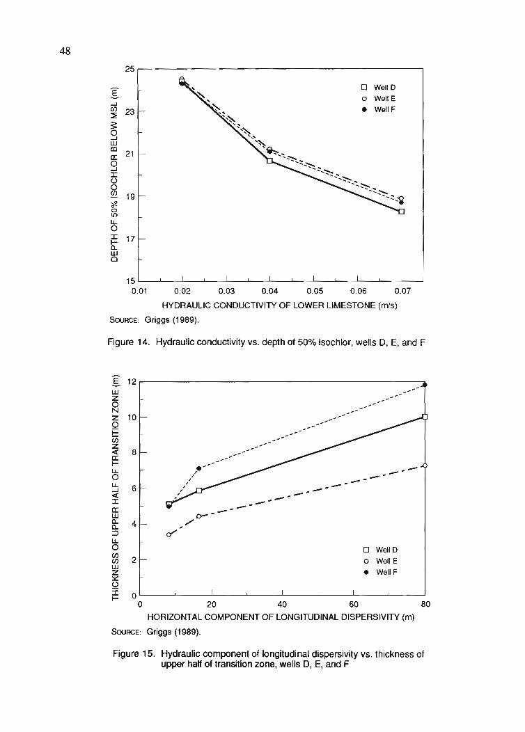
48
25
E 0 Well 0
0 WellE....J(/) 23 • WeliF::::E~0....JUJco
21a:0....J:::c00~ 19~0010U.0:::c 17I-a..UJ0
15 '-----..J_---L_--'-_--'-_-'-_....L-_-'--_.J...-_~____J'_____L_ ____'__ ___'
0.01 0.02 0.03 0.04 0.05 0.06 0.07
HYDRAULIC CONDUCTIVITY OF LOWER LIMESTONE (mls)
SouRCE: Griggs (1989).
Figure 14. Hydraulic conductivity vs. depth of 50% isochlor, wells D, E, and F
E 12r--------------------------..
80
o WeliO
o WellE
• WeliF
---------------------0--/'4
2
8
O'----.J...---..l-.--..l-.--....L----'----'-----'---~
o
6
20 40 60
HORIZONTAL COMPONENT OF LONGITUDINAL DISPERSIVITY (m)
SouRCE: Griggs (1989).
UJz2z 10oi=(j)z«a:Iu.oU.....J«:::ca:UJa..a..:::>u.o(/)(/)UJZ:ll::Q:::cI-
Figure 15. Hydraulic component of longitudinal dispersivity vs. thickness ofupper half of transition zone, wells D, E, and F
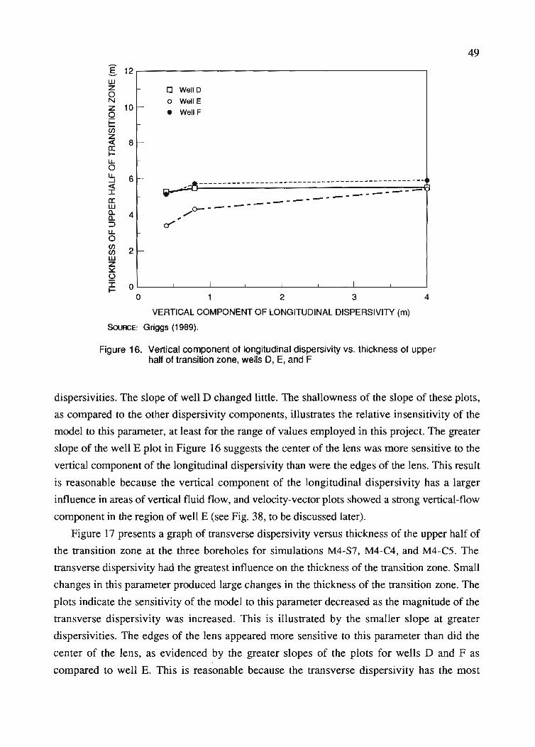
49
I 12~------------------------,
4
,~-----------------------------------------------~
o WeliD
o Well E
• Well F
----------------------0--------,/,
if'
2f-
6f-
8f-
wz2z 10 fai=enz«a:r-u.au...J«J:a:wa..a..=>u.a(/)(/)wz~()
Ir-o1...-__.1--.__.1--.1 _--1__--11__--1__---1.1__---1.__-..1
o 1 2 3
VERTICAL COMPONENT OF LONGITUDINAL DISPERSIVITY (m)
SouRCE: Griggs (1989).
Figure 16. Vertical component of longitudinal dispersivity vs. thickness of upperhalf of transition zone, wells 0, E, and F
dispersivities. The slope of well D changed little. The shallowness of the slope of these plots,
as compared to the other dispersivity components, illustrates the relative insensitivity of the
model to this parameter, at least for the range of values employed in this project. The greater
slope of the well E plot in Figure 16 suggests the center of the lens was more sensitive to the
vertical component of the longitudinal dispersivity than were the edges of the lens. This result
is reasonable because the vertical component of the longitudinal dispersivity has a larger
influence in areas of vertical fluid flow, and velocity-vector plots showed a strong vertical-flow
component in the region of well E (see Fig. 38, to be discussed later).
Figure 17 presents a graph of transverse dispersivity versus thickness of the upper half of
the transition zone at the three boreholes for simulations M4-S7, M4-C4, and M4-C5. The
transverse dispersivity had the greatest influence on the thickness of the transition zone. Small
changes in this parameter produced large changes in the thickness of the transition zone. The
plots indicate the sensitivity of the model to this parameter decreased as the magnitude of the
transverse dispersivity was increased. This is illustrated by the smaller slope at greater
dispersivities. The edges of the lens appeared more sensitive to this parameter than did the
center of the lens, as evidenced by the greater slopes of the plots for wells D and F as
compared to well E. This is reasonable because the transverse dispersivity has the most
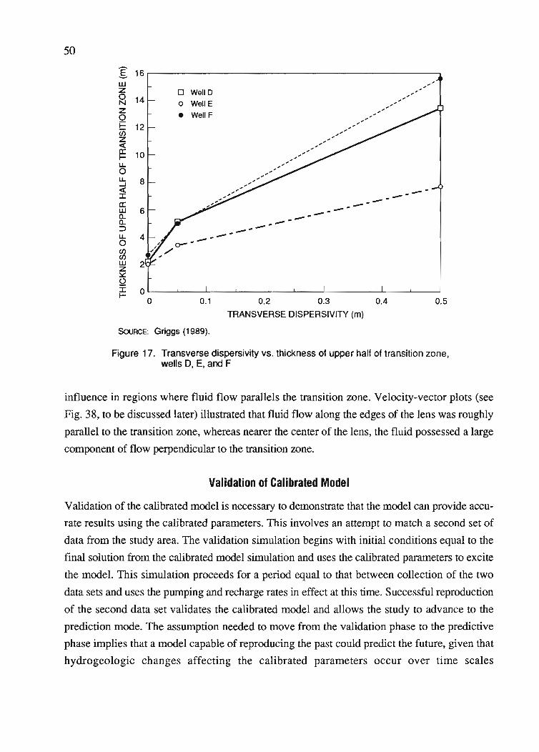
----------------------
WallO
WellE
WallF
0.1 0.2 0.3 0.4 0.5
TRANSVERSE DISPERSIVITY (m)
50
E 16wz 00 14N 0Z •0E 12(/)zor:(II: 10l-LL0u. 8...Jor:(::I:II:W 6a..a..:::lLL 40(/)(/)w 2z~
0I 0I-
0
SouRCE: Griggs (1989).
Figure 17. Transverse dispersivity vs. thickness of upper half of transition zone,wells D, E, and F
influence in regions where fluid flow parallels the transition zone. Velocity-vector plots (see
Fig. 38, to be discussed later) illustrated that fluid flow along the edges of the lens was roughly
parallel to the transition zone, whereas nearer the center of the lens, the fluid possessed a large
component of flow perpendicular to the transition rone.
Validation of Calibrated Model
Validation of the calibrated model is necessary to demonstrate that the model can provide accu
rate results using the calibrated parameters. This involves an attempt to match a second set of
data from the study area. The validation simulation begins with initial conditions equal to the
final solution from the calibrated model simulation and uses the calibrated parameters to excite
the model. This simulation proceeds for a period equal to that between collection of the two
data sets and uses the pumping and recharge rates in effect at this time. Successful reproduction
of the second data set validates the calibrated model and allows the study to advance to the
prediction mode. The assumption needed to move from the validation phase to the predictive
phase implies that a model capable of reproducing the past could predict the future, given that
hydrogeologic changes affecting the calibrated parameters occur over time scales
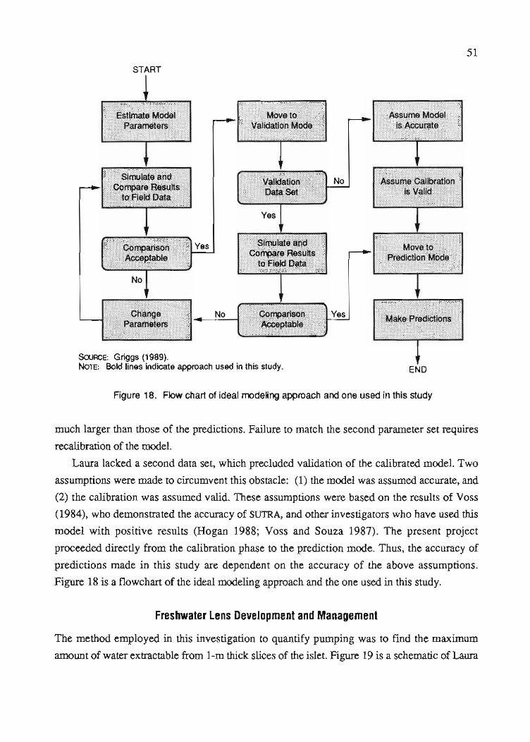
51
START
END
No
......-:.=..--1_ Yes
SouRCE: Griggs (1989).NoTE: Bold lines indicate approach used in this study.
Yes
No
Figure 18. Flow chart of ideal modeling approach and one used in this study
much larger than those of the predictions. Failure to match the second parameter set requires
recalibration of the model.
Laura lacked a second data set, which precluded validation of the calibrated model. Two
assumptions were made to circumvent this obstacle: (1) the model was assumed accurate, and
(2) the calibration was assumed valid. These assumptions were based on the results of Voss
(1984), who demonstrated the accuracy of SUTRA, and other investigators who have used this
model with positive results (Hogan 1988; Voss and Souza 1987). The present project
proceeded directly from the calibration phase to the prediction mode. Thus, the accuracy of
predictions made in this study are dependent on the accuracy of the above assumptions.
Figure 18 is a flowchart of the ideal modeling approach and the one used in this study.
Freshwater Lens Development and Management
The method employed in this investigation to quantify pumping was to find the maximum
amount of water extractable from 1-m thick slices of the islet. Figure 19 is a schematic of Laura
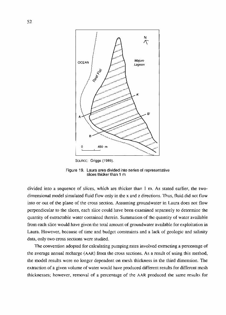
52
o 450 m
N
1\
MajuroLagoon
SouRCE: Griggs (1989).
Figure 19. Laura area divided into series of representativeslices thicker than 1 m
divided into a sequence of slices, which are thicker than I m. As stated earlier, the two
dimensional model simulated fluid flow only in the x and z directions. Thus, fluid did not flow
into or out of the plane of the cross section. Assuming groundwater in Laura does not flow
perpendicular to the slices, each slice could have been examined separately to determine the
quantity of extractable water contained therein. Summation of the quantity of water available
from each slice would have given the total amount of groundwater available for exploitation in
Laura. However, because of time and budget constraints and a lack of geologic and salinity
data, only two cross sections were studied.
The convention adopted for calculating pumping rates involved extracting a percentage of
the average annual recharge (AAR) from the cross sections. As a result of using this method,
the model results were no longer dependent on mesh thickness in the third dimension. The
extraction of a given volume of water would have produced different results for different mesh
thicknesses; however, removal of a percentage of the AAR produced the same results for

53
different thicknesses because the extraction rate changed in proportion to the change in mesh
thickness.
The criteria for a superior development scheme stipulated that the new pumping scenario
had to produce either an equal volume of fresh water with less upconing or a greater quantity of
potable water with more, though acceptable, upconing. Upconing refers to the shape and
decreasing depth of salinity contours as a result of pumping in coastal aquifers. The
quantification of upconing was based on the determination of the shallowest depth of the top of
the saline cone, not on the area of the cone. The following analysis consisted of the comparison
of the depths to the top of the cones to distinguish between superior and inferior development
schemes.
The simulations discussed in this section all reached steady state. Considerations involved
in determining the condition of steady state conformed to those presented earlier in this report.
Initial conditions for each simulation were the final solution from M4-C5, unless stated
otherwise.
WELL DEPTH. The first three pumping simulations that used mesh 4 entailed the extraction
of water from a single node located at different depths. (Extraction nodes are referred to as
wells throughout this report.) The extraction rate was 20% of the AAR, and the simulations
lasted for 2 yr of simulated time. Each well occupied one of three nodes above the 2.6%
isochlor: (1) at the surface of the cross section for simulation M4-PI, (2) 0.76 m below the
surface of the cross section for simulation M4-P2, and (3) 1.52 m below the surface of the
cross section for simulation M4-P3. The node nearest the 2.6% salinity contour directly below
the well became slightly more saline as the depth of the well increased, though the greatest
difference in salinity was 0.04% seawater. Although the greatest well depth was only 1.5 m,
deeper wells would continue to raise the 2.6% isochlor. The shallowest depth of the 2.6%
isochlor was virtually indistinguishable between the simulations and was 9.4 m in each case
(see Fig. 20). The greater well depths caused the potable limit to rise slightly, and these wells
would require more effort to emplace in the field. Therefore, subsequent simulations employed
extraction nodes at the surface of the cross section.
NUMBER OF WELLS. The objective of an increase in the number of wells was to reduce the
amount of upconing observed in the single-well simulations. The development scheme for
simulation M4-P4 consisted of emplacing two wells. The wells lay 61 m to either side of the
single well, and each extracted 10% of the AAR, for a total of 20%. Figure 21 illustrates the
results of simulation M4-P4. The two-well version showed less upconing than the one-well
simulation. The top of the cone in M4-P4 reached a minimum depth of 10.9 m, as compared to
9.4 m for M4-Pl.
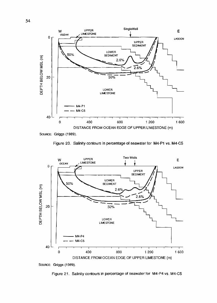
54
o
I-..IC/)
::::E~
9w 20co:cI-Q.Wo
WOCEAN
UPPERLIMESTONE
LOWERLIMESTONE
SingleWellE
LAGOON
- M4-P1
-- M4-C5
40
o 400 800 1 200 1 600
DISTANCE FROM OCEAN EDGE OF UPPER LIMESTONE (m)
SouRCE: Griggs (1989).
Figure 20. Salinity contours in percentage of seawater for M4-P1 vs. M4-C5
WTwo Wells
EOCEAN
0 LAGOON
LOWER
ISEDIMENT
-..IC/)
::::E~0-..I 20 50%wco:cI-Q. LOWERW0 LIMESTONE
-M4-P4
-- M4-C5
40 i
0 400 800 1 200 1 600
DISTANCE FROM OCEAN EDGE OF UPPER LIMESTONE (m)
SouRCE: Griggs (1989).
Figure 21. Salinity contours in percentage of seawater for M4-P4 VS. M4-C5
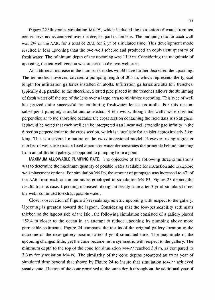
55
Figure 22 illustrates simulation M4-P5, which included the extraction of water from ten
consecutive nodes centered over the deepest part of the lens. The pumping rate for each well
was 2% of the AAR, for a total of 20% for 2 yr of simulated time. This development mode
resulted in less upconing than the two-well scheme and produced an equivalent quantity of
fresh water. The minimum depth of the upconing was 11.9 m. Considering the magnitude of
upconing, the ten-well version was superior to the two-well case.
An additional increase in the number of nodes would have further decreased the upconing.
The ten nodes, however, covered a pumping length of 305 m, which represents the typical
length for infiltration galleries installed on atolls. Infiltration galleries are shallow trenches,
typically dug parallel to the shoreline. Slotted pipe placed in the trenches allows the skimming
of fresh water off the top of the lens over a large area to minimize upconing. This type of well
has proved quite successful for exploiting freshwater lenses on atolls. For this reason,
subsequent pumping simulations consisted of ten wells, though the wells were oriented
perpendicular to the shoreline because the cross section containing the field data is so aligned.
It should be noted that each well can be interpreted as a linear well extending to infinity in the
direction perpendicular to the cross section, which is unrealistic for an islet approximately 3 km
long. This is a severe limitation of the two-dimensional model. However, using a greater
number of wells to extract a fixed amount of water demonstrates the principle behind pumping
from an infiltration gallery, as opposed to pumping from a point.
MAXIMUM ALLOWABLE PUMPING RATE. The objective of the following three simulations
was to determine the maximum quantity of potable water available for extraction and to explore
well-placement options. For simulation M4-P6, the amount of pumpage was increased to 4% of
the AAR from each of the ten nodes employed in simulation M4-P5. Figure 23 depicts the
results for this case. Upconing increased, though at steady state after 3 yr of simulated time,
the wells continued to extract potable water.
Closer observation of Figure 23 reveals asymmetric upconing with respect to the gallery.
Upconing is greatest toward the lagoon. Considering that the low-permeability sediments
thicken on the lagoon side of the islet, the following simulation consisted of a gallery placed
152.4 m closer to the ocean in an attempt to reduce upconing by pumping above more
permeable sediments. Figure 24 compares the results of the original gallery location to the
outcome of the new gallery position after 3 yr of simulated time. The magnitude of the
upconing changed little, yet the cone became more symmetric with respect to the gallery. The
minimum depth to the top of the cone for simulation M4-P7 reached 3.4 m, as compared to
3.3 m for simulation M4-P6. The similarity of the cone depths prompted an extra year of
simulated time beyond that shown by Figure 24 to insure that simulation M4-P7 achieved
steady state. The top of the cone remained at the same depth throughout the additional year of
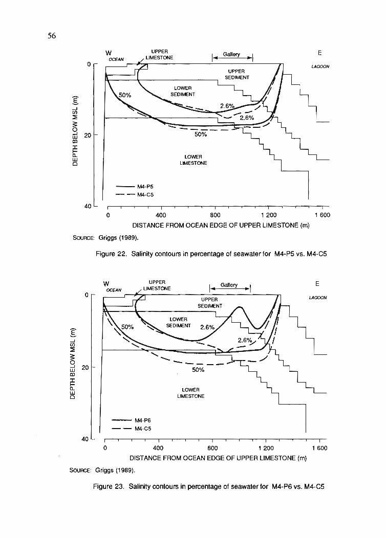
56
o
:[..Jf/)
::E;:oLa 20co
~wCl
WOCEAN
UPPERLIMESTONE
50%
LOWERLIMESTONE
Gallery .1 E
40
-M4-P5--M4-C5
o 400 800 1 200 1 600
DISTANCE FROM OCEAN EDGE OF UPPER LIMESTONE (m)
SouRCE: Griggs (1989).
Figure 22. Salinity contours in percentage of seawater for M4-P5 vs. M4-C5
o
:[..Jf/)
::E;:oLa 20co
~wCl
40
WOCEAN
- M4-P6
-- M4-C5
50%
LOWERLIMESTONE
E
LAGOON
o 400 800 1 200 1 600
DISTANCE FROM OCEAN EDGE OF UPPER LIMESTONE (m)
SouRCE: Griggs (1989).
Figure 23. Salinity contours in percentage of seawater for M4-P6 VS. M4-C5
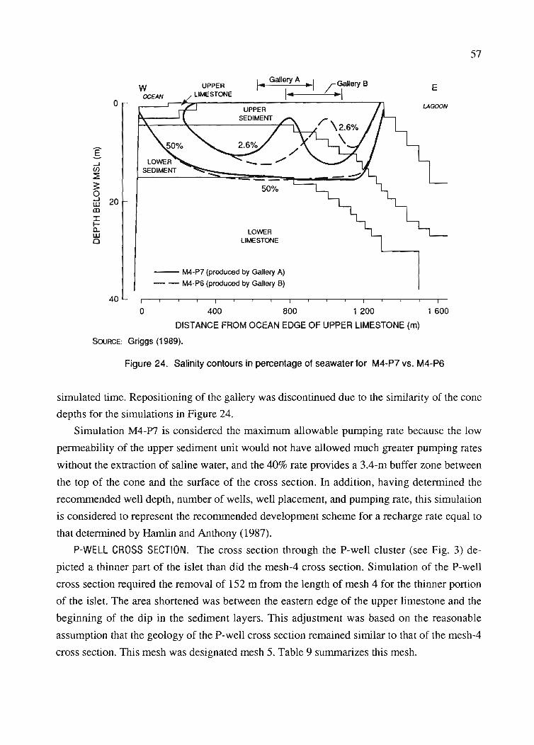
o
..JC/)
::E~ou:l 20CDJ:Ia..LUCl
WOCEAN
I... Gallery A I..__-=-_~~ ~GaIleryB
I... ~I
50%
LOWERLIMESTONE
E
LAGOON
57
40
-- M4-P7 (produced by Gallery A)- - M4-P6 (produced by Gallery B)
o 400 800 1 200 1 600DISTANCE FROM OCEAN EDGE OF UPPER LIMESTONE (m)
SouRCE: Griggs (1989).
Figure 24. Salinity contours in percentage of seawater for M4-P7 vs. M4-P6
simulated time. Repositioning of the gallery was discontinued due to the similarity of the conedepths for the simulations in Figure 24.
Simulation M4-P7 is considered the maximum allowable pumping rate because the lowpermeability of the upper sediment unit would not have allowed much greater pumping rateswithout the extraction of saline water, and the 40% rate provides a 3.4-m buffer zone betweenthe top of the cone and the surface of the cross section. In addition, having determined therecommended well depth, number of wells, well placement, and pumping rate, this simulationis considered to represent the recommended development scheme for a recharge rate equal tothat detennined by Hamlin and Anthony (1987).
P-WELL CROSS SECTION. The cross section through the P-well cluster (see Fig. 3) depicted a thinner part of the islet than did the mesh-4 cross section. Simulation of the P-wellcross section required the removal of 152 m from the length of mesh 4 for the thinner portionof the islet. The area shortened was between the eastern edge of the upper limestone and thebeginning of the dip in the sediment layers. This adjustment was based on the reasonableassumption that the geology of the P-well cross section remained similar to that of the mesh-4cross section. This mesh was designated mesh 5. Table 9 summarizes this mesh.
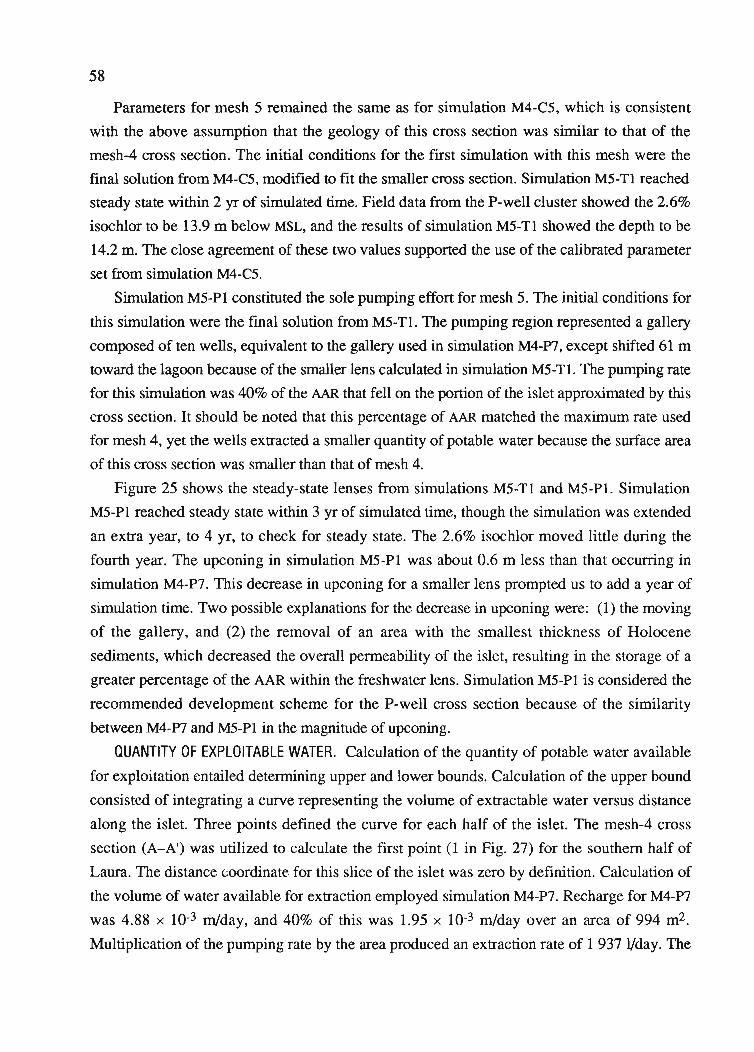
58
Parameters for mesh 5 remained the same as for simulation M4-C5, which is consistent
with the above assumption that the geology of this cross section was similar to that of the
mesh-4 cross section. The initial conditions for the fIrst simulation with this mesh were the
final solution from M4-C5, modified to fIt the smaller cross section. Simulation M5-Tl reached
steady state within 2 yr of simulated time. Field data from the P-well cluster showed the 2.6%
isochlor to be 13.9 m below MSL, and the results of simulation M5-Tl showed the depth to be
14.2 m. The close agreement of these two values supported the use of the calibrated parameter
set from simulation M4-C5.
Simulation M5-Pl constituted the sole pumping effort for mesh 5. The initial conditions for
this simulation were the final solution from M5-Tl. The pumping region represented a gallery
composed of ten wells, equivalent to the gallery used in simulation M4-P7, except shifted 61 m
toward the lagoon because of the smaller lens calculated in simulation M5-Tl. The pumping rate
for this simulation was 40% of the AAR that fell on the portion of the islet approximated by this
cross section. It should be noted that this percentage of AAR matched the maximum rate used
for mesh 4, yet the wells extracted a smaller quantity of potable water because the surface area
of this cross section was smaller than that of mesh 4.
Figure 25 shows the steady-state lenses from simulations M5-Tl and M5-Pl. Simulation
M5-Pl reached steady state within 3 yr of simulated time, though the simulation was extended
an extra year, to 4 yr, to check for steady state. The 2.6% isochlor moved little during the
fourth year. The upconing in simulation M5-Pl was about 0.6 m less than that occurring in
simulation M4-P7. This decrease in upconing for a smaller lens prompted us to add a year of
simulation time. Two possible explanations for the decrease in upconing were: (1) the moving
of the gallery, and (2) the removal of an area with the smallest thickness of Holocene
sediments, which decreased the overall permeability of the islet, resulting in the storage of a
greater percentage of the AAR within the freshwater lens. Simulation M5-Pl is considered the
recommended development scheme for the P-well cross section because of the similarity
between M4-P7 and M5-Pl in the magnitude of upconing.
QUANTITY OF EXPLOITABLE WATER. Calculation of the quantity of potable water available
for exploitation entailed determining upper and lower bounds. Calculation of the upper bound
consisted of integrating a curve representing the volume of extractable water versus distance
along the islet. Three points defined the curve for each half of the islet. The mesh-4 cross
section (A_A') was utilized to calculate the fIrst point (l in Fig. 27) for the southern half of
Laura. The distance (;oordinate for this slice of the islet was zero by definition. Calculation of
the volume of water available for extraction employed simulation M4-P7. Recharge for M4-P7
was 4.88 x 10⁻³ m/day, and 40% of this was 1.95 x 10⁻³ m/day over an area of 994 m2.
Multiplication of the pumping rate by the area produced an extraction rate of 1 937 1/day. The

W UPPER GalleryOCEAN LIMESTONE I~ ~I
0UPPER
SEDIMENT
E--IC/)
~
3=0 50%-I 20LUm::I:....
LOWERa..LU LIMESTONEQ
-- MS-P1
-- MS-T1
40
E
59
o 400 800 1 200 1 600
DISTANCE FROM OCEAN EDGE OF UPPER LIMESTONE (m)
SouRCE: Griggs (1989).
Figure 25. Salinity contours in percentage of seawater for M5-T1 vs. M5-P1
2 OOO~ __
-- Southern half
- - Northern half
>; 1 600co~LU 1 200....<l::a:C'~ 800a..~:::>a..
400
"""""""""" ...." .... .... .... .... ....
........ 3N.. ..... ..... ..... ..... ..... ..... ..... ..... .....
2N0L-_-'---~----'-_.l..-_-'----'---'--_...1---4f...'e---'
o 200 400 600 800 2S 1 000
DISTANCE FROM MESH 4 CROSS SECTION (m)
SouRCE: Griggs (1989).
Figure 26. Curves integrated to obtain quantity of exploitable water
60
coordinates for the first point were 1 937 Vday and zero distance from the mesh-4 cross section
(see Fig. 26).
The second point (25 in Fig. 27) is defIned by the southern limit of potable water, the 2.6%
salinity contour. This contour defined the limit for the installation of wells. Wells placed
outside the 2.6% salinity contour would withdraw nonpotable water. The southern end of the
potable limit contour, shown in Figure 27, was used as the point at which pumpage was zero
for the southern half of the islet. Simulation of a cross section approximating the slice of the
islet containing this point and parallel to the mesh-4 cross section would have resulted in the
withdrawal of only unpotable water. This point plotted at zero pumpage and a distance of
914 m from the mesh-4 cross section (see Fig. 26).
The P-well cross section (B-B') was used to determine the third point (35 in Fig. 27) for
the southern portion of Laura. The distance between this cross section and the mesh-4 cross
section was 486 m. Derivation of the quantity of exploitable water available from this slice of
the islet utilized simulation M5-Pl and the same method as for the first point. The P-well cross
section produced an extraction rate of 1 640 Vday from an area of 842 m2. The coordinates for
point three were 1 640 Vday at a distance of 486 m from the mesh-4 cross section (see
Fig. 26).
Integration to obtain the area below the curve defined by the three points gave the maximum
amount of water available for extraction from the southern half of Laura. The calculation of the
amount of water required a function to integrate over the limits 0.0 m to 914.0 m. A quadratic
equation of the form
a + b(x) + C(X)2 = Y (1)
is required to describe a general curve defined by three points. The simultaneous solution of
equation (1) at the three known points on the curve provided the constants a, b, and c needed to
obtain the required function. The calculations were performed in units of liters per day. For the
sake of clarity, units were omitted in the following calculations.
Substitution of the coordinates of point one in equation (1) produced
a + b(O) + c(Of= 1937 (2)
and a = 1937. Using the results of equation (2), the solution of equation (1) for point two
produced
1937 + b(914) + c(914)2 =0 (3)
and b = -2.12 - 914c. Substitution of the coordinates for point three and the results from
equations (2) and (3) into equation (1) produced
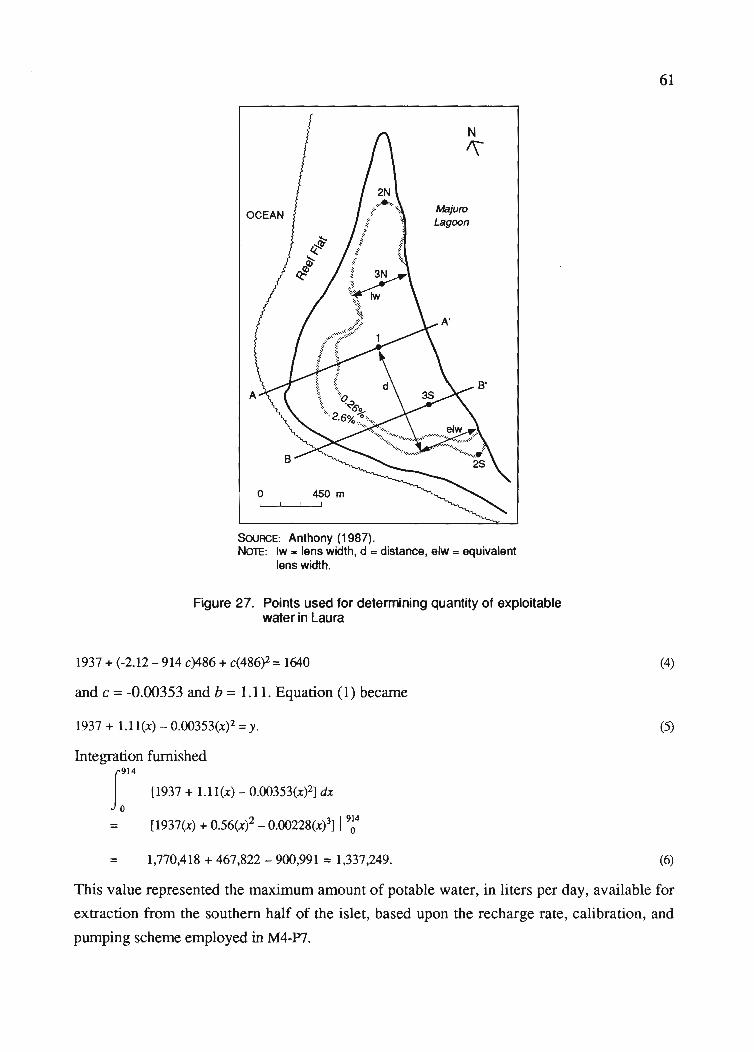
61
OCEAN
oI
450mI
N
1\
MajuroLagoon
SouRCE: Anthony (1987).NoTE: Iw '"' lens width, d =distance, elw =equivalent
lens width.
Figure 27. Points used for determining quantity of exploitablewater in Laura
1937 + (-2.12 - 914 c)486 + c(486)2 =1640
and c =-0.00353 and b =1.11. Equation (1) became
1937 + 1.11(x) - 0.OO353(x)2 = y.
Integration furnished
fo914
(1937 + 1.l1(x) - 0.OO353(x)2] dx
= [1937(x) + 0.56(x)2 _ 0.OO228(x?] I 9~4
(4)
(5)
= 1.770,418 + 467.822 - 900,991 =1,337,249. (6)
This value represented the maximum amount of potable water, in liters per day, available forextraction from the southern half of the islet, based upon the recharge rate, calibration, andpumping scheme employed in M4-P7.
62
The northern portion of the lens appeared smaller than the southern part, based on dug-well
observations (see Fig. 27). The area enclosed by the intersection of the potable limit contour
with the water table in the southern half of the island was larger than the region encompassed
by this contour in the northern half. Simply doubling the allowable extraction rate calculated for
the southern half would have produced too large a value. Determination of the quantity of
exploitable water in the northern half of the islet required a separate solution to equation (1),
using information about pumping rates obtained from simulations of the southern half of the
islet. Derivation of the constants a, b, and c proceeded in the same manner as for the southern
part of the lens.
Calculation of the volume of potable water available for extraction from the northern half of
the islet required three points to define a curve under which to integrate. The first point was the
first point from the curve for the southern half of the islet (see Fig. 26). The second point (2N
in Fig. 27) was an extrapolation of the northern end on the 0.26% isochlor determined by
Anthony (1987). The 0.26% isochlor was used because of a lack of data on the 2.6% isochlor
in this area (see Fig. 27). Using the 0.26% isochlor enabled us to make a conservative estimate
of the extent of the potable lens. The coordinates for the second point were zero pumpage at a
distance of 952 m from the mesh-4 cross section (see Fig. 26).
The third point (3N in Fig. 27), taken midway between the two points, fell at a distance of
476 m from the mesh-4 cross section. Calculation of the pumping rate for point three consisted
of determining the width of the extrapolated potable lens along a line parallel to and 476 m
north of the mesh-4 cross section, finding the distance from the mesh-4 cross section to an
equivalent lens width in the southern half of the islet, and calculating, with equation (5), the
pumping rate at this distance. Figure 27 illustrates the lens width, equivalent lens width, and
distance used to determine the pumping rate. The result was 700 Vday. This point plotted at a
pumpage of 700 Vday and a distance of 476 m (see Fig. 26).
Solution of equation (1) for point one from the northern portion of the lens furnished
a + b(O) + c(O)2= 1937 (7)
and a = 1937. Substitution of the solution for equation (7) and the coordinates for point two in
equation (1) produced
1937 + b(952) + c(952)2 = 0 (8)
and b = -2.03 - 952c. Employing the results from equations (7) and (8), the solution of
equation (1) for point three produced
1937 + (-2.03 - 952c)476 + c(476)2 = 700
and c =0.00107 and b =-3.05. Equation (1) became
(9)
1937 - 3.05(x) + O.OO107(x)2 =y.
Integration furnished
f0
952[1937 - 3.05(x) + O.OO107(x)2)dx
63
(10)
=
=
[1937(x) - 1.53(x)2 + O.OOO36(x)3) I~2
1,844,024 - 1,386,645 + 310,609 =767,988. (11)
This number was the maximum quantity of potable water, in liters per day, available for
exploitation from the northern half of the islet. The total for the islet was approximately 2.1
million l/day, or 30% of the average daily recharge to the lens calculated by Hamlin and
Anthony (1987). This compared favorably with the estimate given by Anthony (1987) of
roughly 1.5 million l/day, or 22% of the average daily recharge to the lens. It should be noted
that the value determined above represents a maximum because the method used to calculate it
included the assumption that each I-m slice of the islet contained a gallery of ten wells and was
independent of the other slices.
Calculation of the lower bound for the quantity of potable water available for exploitation
from Laura involved the use of simulation M4-Pl (see Tab. 11 and Fig. 20). The magnitude of
upconing in this simulation was less than that of M4-P7, which indicated M4-Pl demonstrated
an acceptable development and management scheme. For the calculation of the minimum
quantity of exploitable water, Laura was assumed to represent an infinite strip and simulation
M4-Pl was interpreted as representing a gallery extending the full length of the islet. The lens
near the ends of the islet would not have sustained extraction of 20% of the AAR because the
islet narrows, and the assumption of an infinite strip is invalid in these areas. However, the
center of the lens would have allowed a greater extraction rate while maintaining an acceptable
amount of upconing. Thus, it is believed, based on M4-Pl, an average pumping rate of 20% is
possible and the extraction of 20% of the AAR represents a lower bound for Laura. In other
words, at least 20% of the AAR can be extracted. This is approximately 1.4 million I of fresh
water per day at the recharge rate determined by Hamlin and Anthony (1987).
Influence of Recharge on Pumping
The goal of the following three simulations was to examine the effect of changes in the
recharge rate. The first simulation included a change in the recharge rate from the AAR to
average monthly recharge (AMR) values. The second and third simulations consisted of an
analysis of the effect of a severe drought on the freshwater lens in Laura, using two different
pumping rates.
64
AVERAGE MONTHLY RECHARGE RATES. The recharge rate for simulation M4-P8 was
changed to AMR rates because they more closely approximate the field recharge rate.
Calculation of the percentage of the annual recharge attributable to each month entailed the use
of AMR values recorded on Majuro Atoll since 1955 (u.s. NOAA 1985). The recorded AMR
rates required normalization to the current annual recharge rate because the average annual
rainfall over the duration of the study of Hamlin and Anthony (1987) exceeded the average of
the prior 30 yr. This normalization maintained a total yearly recharge to the freshwater lens
equivalent to the rate used for the previous simulations.
The initial conditions for simulation M4-P8 were the fmal solution from M4-C5. The
simulation began with the August monthly recharge rate because this value most closely
approximated the AAR rate used for the previous simulations. The initial conditions were
closest to steady state for the August recharge rate. In this case, steady state referred to the lens
being in the same condition at the same time each year. The changing recharge rate caused the
solution to change continuously and never reach steady state, as defmed before.
The pumping rate remained constant throughout the year, at 40% of the AAR. The
simulation proceeded for 3 yr of simulated time and generated output every two weeks during
the third year to allow identification of the smallest lens. Figure 28 illustrates the largest amount
of upconing throughout the year. This lens appeared at the end of July.
The results of simulation M4-P8 showed less upconing than determined for M4-P7,
although the areas of the lenses above the 2.6% isochlor were similar. More interestingly,
simulation M4-P8 provided insight into the time the lens took to react to variations in the
recharge rate. The 50% isochlor, which can be interpreted as the boundary of the lens,
responded to changes in recharge after approximately one month (see Fig. 29). The largest lens
appeared in early December, approximately one month after the end of the recharge peak in
October. In addition, the lens began to show growth in July, after the large increase in recharge
in June, and a period of lens stagnation occurred during late August and early September,
nearly one month after the beginning of the August recharge trough. The 2.6% isochlor had a
greater lag time. However, the position of the 2.6% isochlor depends on both the calibrated
permeabilities and dispersivities, whereas the position of the 50% isochlor depends primarily
on the calibrated permeabilities. The dispersivities have a strong influence on reaction times, as
will be illustrated in a later section of this report. Therefore, the 2.6% isochlor is not
considered a good indicator of lens reaction times.
SIMULATED DROUGHT CONDITIONS. The simulated drought conditions approximated the
rainfall measured during the 1982 to 1983 El Nino event, when rainfall records showed a
decrease of approximately 35% in the rainfall rate. Hence, the AAR rate was uniformly reduced
by 35% for the two simulations in this experiment. The initial conditions for simulation M4-P9
65
o
-I(J)
~
3:ou:J 20co:cIa..UJo
WOCEAN
LOWERLIMESTONE
E
LAGOON
--- M4-P8--M4-P7
40o 400 800 1 200 1 600
DISTANCE FROM OCEAN EDGE OF UPPER LIMESTONE (m)
SouRCE: Griggs (1989).
Figure 28. Salinity contours in percentage of seawater for M4-P8 vs. M4-P7
4.5
0.65 8.5
E0.55 :c
:§:I-a..
Recharge UJUJ 0
" UJa:6.5 z
< 0.45 0:c ()()
::EUJa: :::::>
::E
0.35 ~::E
Jan. Feb. Mar. Apr. May Jun. Jul. Aug. Sept. Oct. Nov. Dec.
MONTH
SouRCE: Griggs (1989).
Figure 29. Curves showing delay between changes in the recharge rate andcorresponding change in depth of 50% isochlor
66
were the final solution of M4-P7 to simulate the consequences of a drought beginning after
development of the resource at Laura. The pumping rate for the first drought simulation
remained constant at 40% of the AAR before the drought, which was 62% of the drought
recharge rate.
Figure 30 depicts the lens from M4-P9 after 3 yr of simulated time. Unpotable water entered
the gallery after less than one year. The original extraction rate (40% of AAR) failed as a viable
management scheme for supplying fresh water under severe drought conditions. After 3 yr of
the reduced recharge, the average salinity of the ten nodes forming the gallery was
approximately 7.5% seawater. This exceeded the potable limit for salinity about threefold, yet
in a critical situation, this development and management scheme could provide large quantities
of relatively fresh water, which would require less effort to desalinize than pure seawater.
The pumping rate was decreased to 30% of the AAR before the drought for simulation M4
PlO, which was 46% of the drought recharge. Initial conditions were the final solution from
M4-P7. Figure 31 shows the lens after 3 yr of simulated time. The gallery continued to extract
potable water, though upconing exceeded that of simulation M4-P7. This scheme is considered
unacceptable because the top of the cone is too near the surface. However, these results
indicate the lens beneath Laura can continue to provide significant quantities of potable or low
salinity water during drought periods.
Influence of Calibrated Parameters on Lens Creation and Pumping
This section discusses the influence calibrated parameters had on lens creation and pumping
results. The first subsection covers differences in the length of time needed to create a
freshwater lens, beginning with an islet saturated with seawater. The second subsection
includes results from pumping using two different parameter sets.
LENS CREATION. Simulation M4-C6 consisted of the creation of the freshwater lens using
the calibrated parameter set from M4-C5. The initial conditions were concentrations equal to
seawater and hydrostatic pressures, calculated using a fluid density equivalent to seawater. The
simulation reached steady state within 6 yr of simulated time. This was roughly half the time
needed to form the steady-state lens for simulation M3-Tl(see Tab. 8).
The higher permeability for M4-C6 required less fresh water to recharge the aquifer because
the lens was smaller and stored less water. This accounted for part of the decrease in the time
needed to reach steady state. However, the sensitivity analysis suggested the transport solution
reacted more slowly to large dispersivities since the solute had to be dispersed over greater
distances. The smaller dispersivities in M4-C6 produced the remaining decrease in simulation
time. This indicated the time the model took to react to imposed stresses depended on the
o
I-l(f)
~
~
9 20wIX)
::r:::Ia..wo
40
"-LOWE~ ..........---...;;;;..;.....----~-_=Z~
SEDIMENT """- _
LOWERLIMESTONE
---M4-P9
-- M4-P7
E
67
o 400 800 1 200 1 600
DISTANCE FROM OCEAN EDGE OF UPPER LIMESTONE (m)
SouRCE: Griggs (1989).
Figure 30. Salinity contours in percentage of seawater for M4-P9 VS. M4-P7
o
I-l(f)
~
~
9w 20IX)
::r:::Ia..wo
40
-M4-P10
-- M4-P7
LOWERLIMESTONE
E
LAGOON
o 400 800 1 200 1 600
DISTANCE FROM OCEAN EDGE OF UPPER LIMESTONE (m)
SouRCE: Griggs (1989).
Figure 31. Salinity contours in percentage of seawater for M4-P10 VS. M4-P7
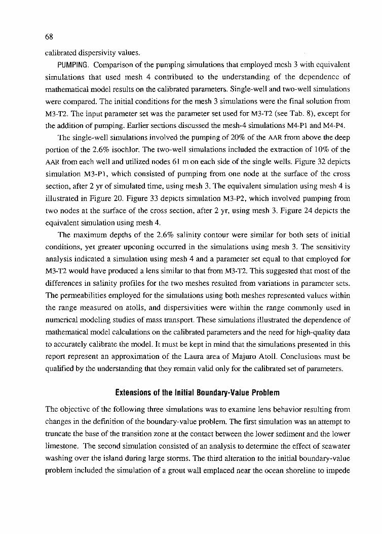
68
calibrated dispersivity values.
PUMPING. Comparison of the pumping simulations that employed mesh 3 with equivalent
simulations that used mesh 4 contributed to the understanding of the dependence of
mathematical model results on the calibrated parameters. Single-well and two-well simulations
were compared. The initial conditions for the mesh 3 simulations were the final solution from
M3-TI. The input parameter set was the parameter set used for M3-TI (see Tab. 8), except for
the addition of pumping. Earlier sections discussed the mesh-4 simulations M4-Pl and M4-P4.
The single-well simulations involved the pumping of 20% of the AAR from above the deep
portion of the 2.6% isochlor. The two-well simulations included the extraction of 10% of the
AAR from each well and utilized nodes 61 m on each side of the single wells. Figure 32 depicts
simulation M3-Pl, which consisted of pumping from one node at the surface of the cross
section, after 2 yr of simulated time, using mesh 3. The equivalent simulation using mesh 4 is
illustrated in Figure 20. Figure 33 depicts simulation M3-P2, which involved pumping from
two nodes at the surface of the cross section, after 2 yr, using mesh 3. Figure 24 depicts the
equivalent simulation using mesh 4.
The maximum depths of the 2.6% salinity contour were similar for both sets of initial
conditions, yet greater upconing occurred in the simulations using mesh 3. The sensitivity
analysis indicated a simulation using mesh 4 and a parameter set equal to that employed for
M3-TI would have produced a lens similar to that from M3-TI. This suggested that most of the
differences in salinity profiles for the two meshes resulted from variations in parameter sets.
The permeabilities employed for the simulations using both meshes represented values within
the range measured on atolls, and dispersivities were within the range commonly used in
numerical modeling studies of mass transport. These simulations illustrated the dependence of
mathematical model calculations on the calibrated parameters and the need for high-quality data
to accurately calibrate the model. It must be kept in mind that the simulations presented in this
report represent an approximation of the Laura area of Majuro Atoll. Conclusions must be
qualified by the understanding that they remain valid only for the calibrated set of parameters.
Extensions of the Initial Boundary-Value Problem
The objective of the following three simulations was to examine lens behavior resulting from
changes in the defmition of the boundary-value problem. The first simulation was an attempt to
truncate the base of the transition zone at the contact between the lower sediment and the lower
limestone. The second simulation consisted of an analysis to determine the effect of seawater
washing over the island during large storms. The third alteration to the initial boundary-value
problem included the simulation of a grout wall emplaced near the ocean shoreline to impede
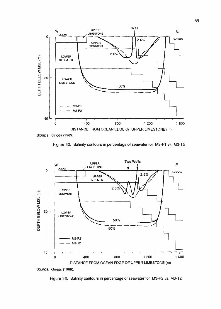
69Well
50%
............ ---------
- M3-P1
-- M3-P2
LOWERSEDIMENT
LOWERLIMESTONE
WOCEANo
g-lC/)
::E~ou:J 20co:cb:wo
40 I I Io 400 800 1 200 1 600
DISTANCE FROM OCEAN EDGE OF UPPER LIMESTONE (m)
SouRCE: Griggs (1989).
Figure 32. Salinity contours in percentage of seawater for M3-P1 vs. M3-T2
E
~
~, 50%
-------_./50%
- M3-P2
-- M3-T2
LOWERSEDIMENT
LOWERLIMESTONE
WOCEANo
g-lC/)
::E~
9 20wco:cb:wo
40 I I Io 400 800 1 200 1 600
DISTANCE FROM OCEAN EDGE OF UPPER LIMESTONE (m)
SouRCE: Griggs (1989).
Figure 33. Salinity contours in percentage of seawater for M3-P2 vs. M3-T2
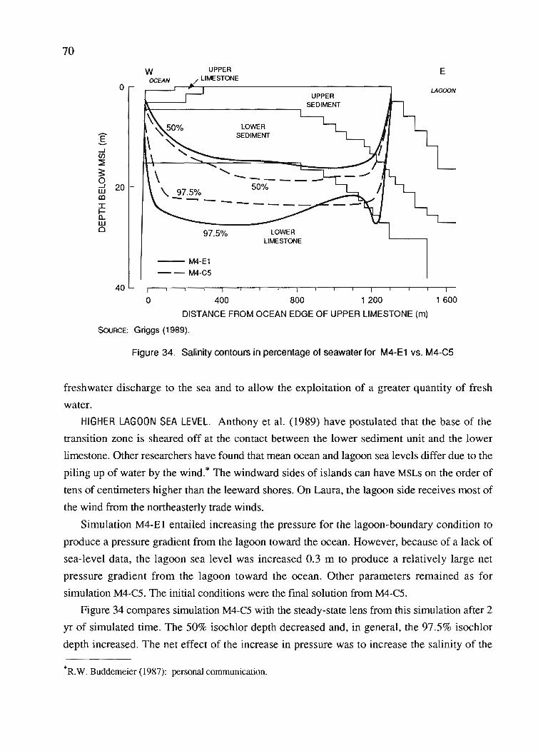
70
o
g-l(/)
::E~om 20co
~a..wCl
WOCEAN
UPPERLIMESTONE
LOWERSEDIMENT
97.5% LOWERLIMESTONE
E
LAGOON
40
-- M4-El
-- M4-C5
o 400 800 1 200 1 600
DISTANCE FROM OCEAN EDGE OF UPPER LIMESTONE (m)
SouRCE: Griggs (1989).
Figure 34. Salinity contours in percentage of seawater for M4-E1 vs. M4-C5
freshwater discharge to the sea and to allow the exploitation of a greater quantity of fresh
water.
HIGHER LAGOON SEA LEVEL. Anthony et al. (1989) have postulated that the base of the
transition zone is sheared off at the contact between the lower sediment unit and the lower
limestone. Other researchers have found that mean ocean and lagoon sea levels differ due to the
piling up of water by the wind.* The windward sides of islands can have MSLs on the order of
tens of centimeters higher than the leeward shores. On Laura, the lagoon side receives most of
the wind from the northeasterly trade winds.
Simulation M4-E 1 entailed increasing the pressure for the lagoon-boundary condition to
produce a pressure gradient from the lagoon toward the ocean. However, because of a lack of
sea-level data, the lagoon sea level was increased 0.3 m to produce a relatively large net
pressure gradient from the lagoon toward the ocean. Other parameters remained as for
simulation M4-C5. The initial conditions were the [mal solution from M4-C5.
Figure 34 compares simulation M4-C5 with the steady-state lens from this simulation after 2
yr of simulated time. The 50% isochlor depth decreased and, in general, the 97.5% isochlor
depth increased. The net effect of the increase in pressure was to increase the salinity of the
*R.W. Buddemeier (1987): personal communication.
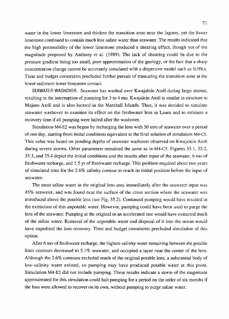
71
water in the lower limestone and thicken the transition zone near the lagoon, yet the lowerlimestone continued to contain much less saline water than seawater. The results indicated thatthe high permeability of the lower limestone produced a shearing effect, though not of themagnitude proposed by Anthony et al. (1989). The lack of shearing could be due to thepressure gradient being too small, poor approximation of the geology, or the fact that a sharpconcentration change cannot be accurately simulated with a dispersive model such as SUTRA.Time and budget constraints precluded further pursuit of truncating the transition zone at thelower sediment-lower limestone contact.
SEAWATER WASHOVER. Seawater has washed over Kwajalein Atoll during large storms,resulting in the interruption of pumping for 3 to 4 mo. Kwajalein Atoll is similar in structure toMajuro Atoll and is also located in the Marshall Islands. Thus, it was decided to simulateseawater washover to examine its effect on the freshwater lens in Laura and to estimate arecovery time if all pumping were halted after the washover.
Simulation M4-E2 was begun by recharging the lens with 50 mm of seawater over a periodof one day, starting from initial conditions equivalent to the final solution of simulation M4-C5.This value was based on ponding depths of seawater washover observed on Kwajalein Atollduring severe storms. Other parameters remained the same as in M4-C5. Figures 35.1, 35.2,35.3, and 35.4 depict the initial conditions and the results after input of the seawater, 6 mo offreshwater recharge, and 1.5 yr of freshwater recharge. This problem required about two yearsof simulated time for the 2.6% salinity contour to reach its initial position before the input ofseawater.
The most saline water in the original lens area immediately after the seawater input was45% seawater, and was found near the surface of the cross section where the seawater wasintroduced above the potable lens (see Fig. 35.2). Continued pumping would have resulted inthe extraction of this unpotable water. However, pumping could have been used to purge thelens of the seawater. Pumping at the original or an accelerated rate would have extracted muchof the saline water. Removal of the unpotable water and disposal of it into the ocean wouldhave expedited the lens recovery. Time and budget constraints precluded simulation of thisoption.
After 6 mo of freshwater recharge, the highest-salinity water remaining between the potablelimit contours decreased to 5.1 % seawater, and occupied a layer near the center of the lens.Although the 2.6% contours excluded much of the original potable lens, a substantial body oflow-salinity water existed, so pumping may have produced potable water at this point.Simulation M4-E2 did not include pumping. These results indicate a storm of the magnitudeapproximated for this simulation could halt pumping for a period on the order of six months ifthe lens were allowed to recover on its own, without pumping to purge saline water.
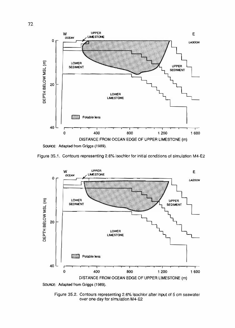
72
o
40
WOCEAN
LOWERSEDIMENT
I:::::) Potable lens
LOWERLIMESTONE
E
LAGOON
o 400 800 1 200 1 600
DISTANCE FROM OCEAN EDGE OF UPPER LIMESTONE (m)
SOURCE: Adapted from Griggs (1989).
Figure 35.1. Contours representing 2.6% isochlor for initial conditions of simulation M4-E2
o
I...JC/)
~
==g 20UJmJ:
6:UJCl
40
wOCEAN
LOWERSEDIMENT
ttl Potable lens
LOWERLIMESTONE
E
LAGOON
o 400 800 1 200 1 600
DISTANCE FROM OCEAN EDGE OF UPPER LIMESTONE (m)
SOURCE: Adapted from Griggs (1989).
Figure 35.2. Contours representing 2.6% isochlor after input of 5 cm seawaterover one day for simulation M4-E2
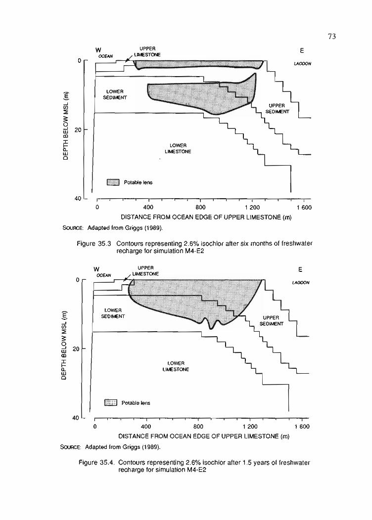
o
I-J(/)
~
:=ou:l 20CDJ:
li:wo
40
WOCEAN
LOWERSEDIMENT
@i>~{1 Potable lens
LOWERLIMESTONE
E
LAGOON
73
o 400 800 1 200 1 600
DISTANCE FROM OCEAN EDGE OF UPPER LIMESTONE (m)
SouRCE: Adapted from Griggs (1989).
Figure 35.3 Contours representing 2.6% isochlor after six months of freshwaterrecharge for simulation M4-E2
o
I-J(/)
~
:=ou:l 20CDJ:~Q.Wo
40
WOCEAN
LOWERSEDIMENT
It I Potable lens
LOWERLIMESTONE
E
LAGOON
o 400 800 1 200 1 600
DISTANCE FROM OCEAN EDGE OF UPPER LIMESTONE (m)
SouRCE: Adapted from Griggs (1989).
Figure 35.4. Contours representing 2.6% isochlor after 1.5 years of freshwaterrecharge for simulation M4-E2

74
Figure 35.4 shows the 2.6% contour after 1.5 yr of freshwater recharge. Potable water again
formed an intact lens. The fingering near the greatest depth of the 2.6% isochlor also appeared
at earlier times. This feature evolved from a complex flow field caused by density-dependent
fluid flow. The flow field consisted of a set of transient clockwise and counterclockwise
vortices. The downward extensions of the 2.6% contour formed where vortices met and the
flow direction was downward. (See Voss and Souza [1987] for a more in-depth discussion of
this process.)
GROUT WALL. A grout wall was simulated in an attempt to increase lens storage by
reducing permeability and thereby groundwater-flow rates. The decision to place the grout wall
on the ocean side of the islet was based on the observation that the potable lens was thinnest on
this side of the islet, so a grout wall would have the greatest effect in this area. The depth of the
wall extended to the contact between the lower sediment and lower limestone units because the
lower limestone appeared to be lithified and contain large solution features. Injection of grout
into this unit would require more effort and probably have a small effect on large solution
features. The reason for locating the wall at the edge of the upper limestone was that it would
require more effort to drill through the limestone than it would to drill through unconsolidated
sediments, yet being less thick, the permeable sediment layer below the relatively impermeable
upper limestone could be taken advantage of at the edge of the limestone.
Initial attempts to approximate a grout wall entailed refming the horizontal dimension of the
elements in the area of the mesh near the edge of the upper limestone and assigning a
gradational permeability distribution leading to an inner core of relatively low permeability. The
horizontal dimension was reduced from 30.5 m to 7.6 m for 30.5 m on each side of the edge of
the upper limestone. This mesh was denoted mesh 6, and is described in Table 9.
For simulation M6-G1, the two elements in the center of the refined area of the mesh were
assigned a permeability value three orders of magnitude less than that of the upper sediment.
The three elements on each side of this core had permeabilities 1.5 orders of magnitude less
than that of the upper sediment. The model was unable to simulate this large a permeability
contrast, especially in the lower sediment, as indicated by instabilities near the wall in the form
of negative concentrations and an unrealistic flow regime.
Simulation M6-G2 included a decrease of the core permeability to two orders of magnitude
less than the upper sediment. The three elements on each side of the core had permeabilities one
order of magnitude less than that of the upper sediment unit. Again, the solution produced
negative concentrations and an unrealistic flow regime in the area of the grout wall.
It was felt that a smaller permeability contrast between the grout wall and the upper
sediment unit would fail to represent an effective barrier to fluid flow. Hence, the third attempt
involved a modification of the boundaries of the mesh to approximate the limiting case of an
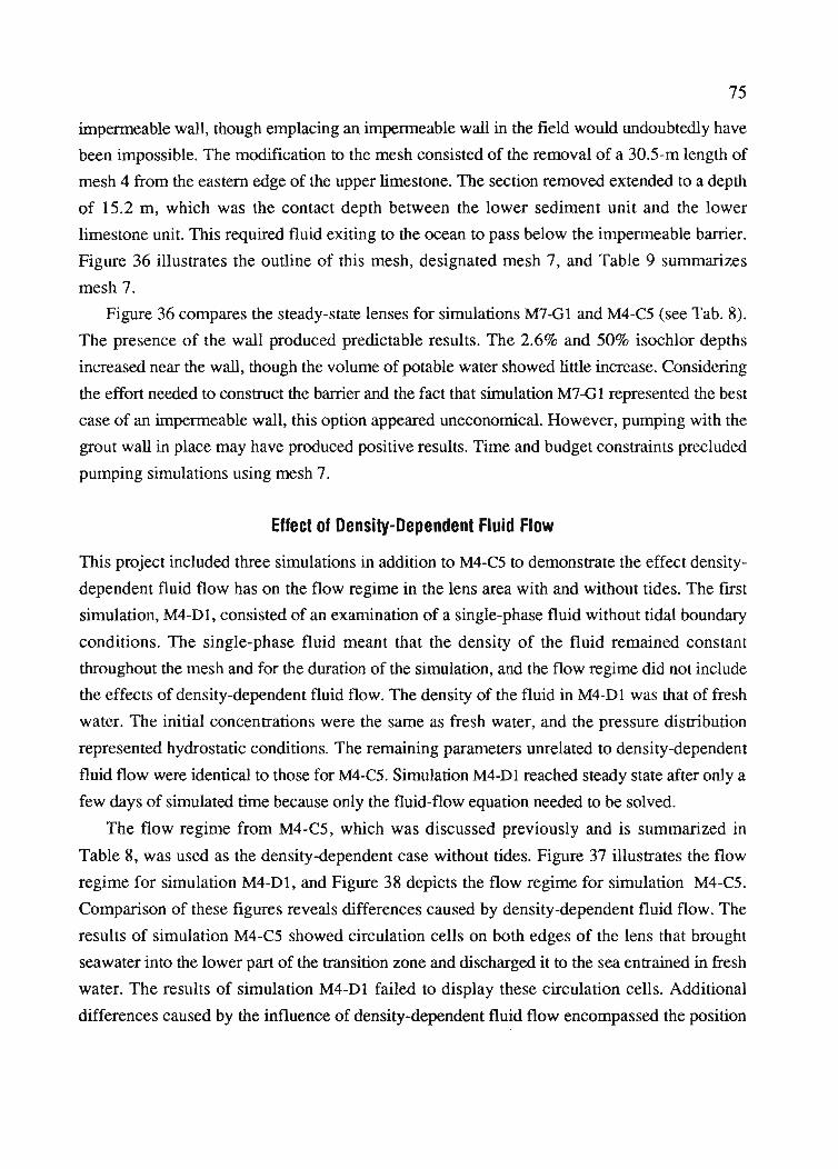
75
impenneable wall, though emplacing an impenneable wall in the field would undoubtedly havebeen impossible. The modification to the mesh consisted of the removal of a 30.5-m length ofmesh 4 from the eastern edge of the upper limestone. The section removed extended to a depthof 15.2 m, which was the contact depth between the lower sediment unit and the lowerlimestone unit. This required fluid exiting to the ocean to pass below the impenneable barrier.Figure 36 illustrates the outline of this mesh, designated mesh 7, and Table 9 summarizesmesh 7.
Figure 36 compares the steady-state lenses for simulations M7-G1 and M4-C5 (see Tab. 8).The presence of the wall produced predictable results. The 2.6% and 50% isochlor depthsincreased near the wall, though the volume of potable water showed little increase. Consideringthe effort needed to construct the barrier and the fact that simulation M7-Gl represented the bestcase of an impenneable wall, this option appeared uneconomical. However, pumping with thegrout wall in place may have produced positive results. Time and budget constraints precludedpumping simulations using mesh 7.
Effect of Density-Dependent Fluid Flow
This project included three simulations in addition to M4-C5 to demonstrate the effect densitydependent fluid flow has on the flow regime in the lens area with and without tides. The firstsimulation, M4-Dl, consisted of an examination of a single-phase fluid without tidal boundaryconditions. The single-phase fluid meant that the density of the fluid remained constantthroughout the mesh and for the duration of the simulation, and the flow regime did not includethe effects of density-dependent fluid flow. The density of the fluid in M4-Dl was that of freshwater. The initial concentrations were the same as fresh water, and the pressure distributionrepresented hydrostatic conditions. The remaining parameters unrelated to density-dependentfluid flow were identical to those for M4-C5. Simulation M4-Dl reached steady state after only afew days of simulated time because only the fluid-flow equation needed to be solved.
The flow regime from M4-C5, which was discussed previously and is summarized inTable 8, was used as the density-dependent case without tides. Figure 37 illustrates the flowregime for simulation M4-Dl, and Figure 38 depicts the flow regime for simulation M4-C5.Comparison of these figures reveals differences caused by density-dependent fluid flow. Theresults of simulation M4-C5 showed circulation cells on both edges of the lens that broughtseawater into the lower part of the transition zone and discharged it to the sea entrained in freshwater. The results of simulation M4-Dl failed to display these circulation cells. Additionaldifferences caused by the influence of density-dependent fluid flow encompassed the position
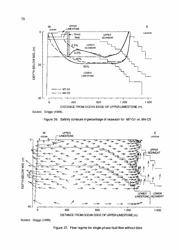
76
o
I...J(/)
::E3:9 20UJcoJ:~a..UJo
40
r-r-i','~Grout1\--\-_-' Wall
I-~-='-------,
50%
LOWER
LIMESTONE
--- M7-Gl
- - M4-C5
E
LAGOON
o 400 800 1 200 1 600
DISTANCE FROM OCEAN EDGE OF UPPER LIMESTONE (m)
SouRCE: Griggs (1989).
Figure 36. Salinity contours in percentage of seawater for M7-G1 vs. M4-C5
LOWER LOWERUMESTONE SEDIMENT
E...J(/)
:::
~UJco
~UJo
o
40 j
o
w
400 800 1200
DISTANCE FROM OCEAN EDGE OF UPPER LIMESTONE (m)
ELAGOON
1600
SouRCE: Griggs (1989).
Figure 37. Flow regime for single-phase fluid flow without tides
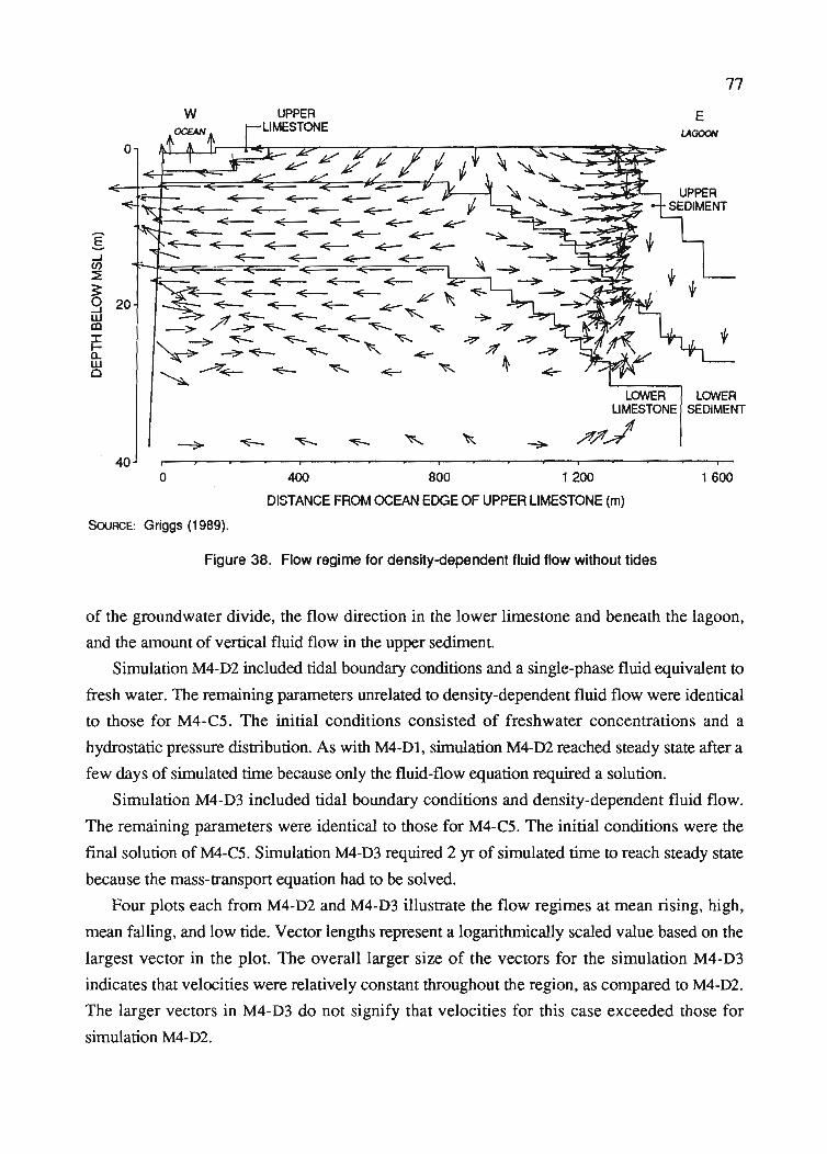
w
o
:[...J
~
~ 20wCD
two
40
77
ELAGOON
LOWER LOWERUMESTONE SEDIMENT
.-#/'~o
SouRCE: Griggs (1989).
~ 800 1200DISTANCE FROM OCEAN EDGE OF UPPER LIMESTONE (m)
1600
Figure 38. Flow regime for density-dependent fluid flow without tides
of the groundwater divide, the flow direction in the lower limestone and beneath the lagoon,and the amount of vertical fluid flow in the upper sediment.
Simulation M4-D2 included tidal boundary conditions and a single-phase fluid equivalent tofresh water. The remaining parameters unrelated to density-dependent fluid flow were identicalto those for M4-C5. The initial conditions consisted of freshwater concentrations and ahydrostatic pressure distribution. As with M4-Dl, simulation M4-D2 reached steady state after afew days of simulated time because only the fluid-flow equation required a solution.
Simulation M4-D3 included tidal boundary conditions and density-dependent fluid flow.The remaining parameters were identical to those for M4-C5. The initial conditions were thefinal solution of M4-C5. Simulation M4-D3 required 2 yr of simulated time to reach steady statebecause the mass-transport equation had to be solved.
Four plots each from M4-D2 and M4-D3 illustrate the flow regimes at mean rising, high,mean falling, and low tide. Vector lengths represent a logarithmically scaled value based on thelargest vector in the plot. The overall larger size of the vectors for the simulation M4-D3indicates that velocities were relatively constant throughout the region, as compared to M4-D2.The larger vectors in M4-D3 do not signify that velocities for this case exceeded those forsimulation M4-D2.
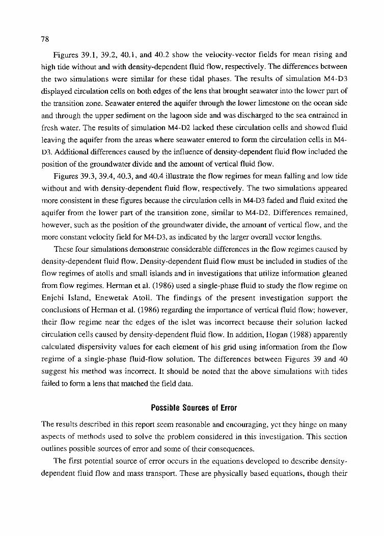
78
Figures 39.1, 39.2, 40.1, and 40.2 show the velocity-vector fields for mean rising and
high tide without and with density-dependent fluid flow, respectively. The differences between
the two simulations were similar for these tidal phases. The results of simulation M4-D3
displayed circulation cells on both edges of the lens that brought seawater into the lower part of
the transition zone. Seawater entered the aquifer through the lower limestone on the ocean side
and through the upper sediment on the lagoon side and was discharged to the sea entrained in
fresh water. The results of simulation M4-D2 lacked these circulation cells and showed fluid
leaving the aquifer from the areas where seawater entered to form the circulation cells in M4
D3. Additional differences caused by the influence of density-dependent fluid flow included the
position of the groundwater divide and the amount of vertical fluid flow.
Figures 39.3, 39.4, 40.3, and 40.4 illustrate the flow regimes for mean falling and low tide
without and with density-dependent fluid flow, respectively. The two simulations appeared
more consistent in these figures because the circulation cells in M4-D3 faded and fluid exited the
aquifer from the lower part of the transition zone, similar to M4-D2. Differences remained,
however, such as the position of the groundwater divide, the amount of vertical flow, and the
more constant velocity field for M4-D3, as indicated by the larger overall vector lengths.
These four simulations demonstrate considerable differences in the flow regimes caused by
density-dependent fluid flow. Density-dependent fluid flow must be included in studies of the
flow regimes of atolls and small islands and in investigations that utilize information gleaned
from flow regimes. Herman et al. (1986) used a single-phase fluid to study the flow regime on
Enjebi Island, Enewetak Atoll. The findings of the present investigation support the
conclusions of Herman et aI. (1986) regarding the importance of vertical fluid flow; however,
their flow regime near the edges of the islet was incorrect because their solution lacked
circulation cells caused by density-dependent fluid flow. In addition, Hogan (1988) apparently
calculated dispersivity values for each element of his grid using information from the flow
regime of a single-phase fluid-flow solution. The differences between Figures 39 and 40
suggest his method was incorrect. It should be noted that the above simulations with tides
failed to form a lens that matched the field data.
Possible Sources of Error
The results described in this report seem reasonable and encouraging, yet they hinge on many
aspects of methods used to solve the problem considered in this investigation. This section
outlines possible sources of error and some of their consequences.
The first potential source of error occurs in the equations developed to describe density
dependent fluid flow and mass transport. These are physically based equations, though their
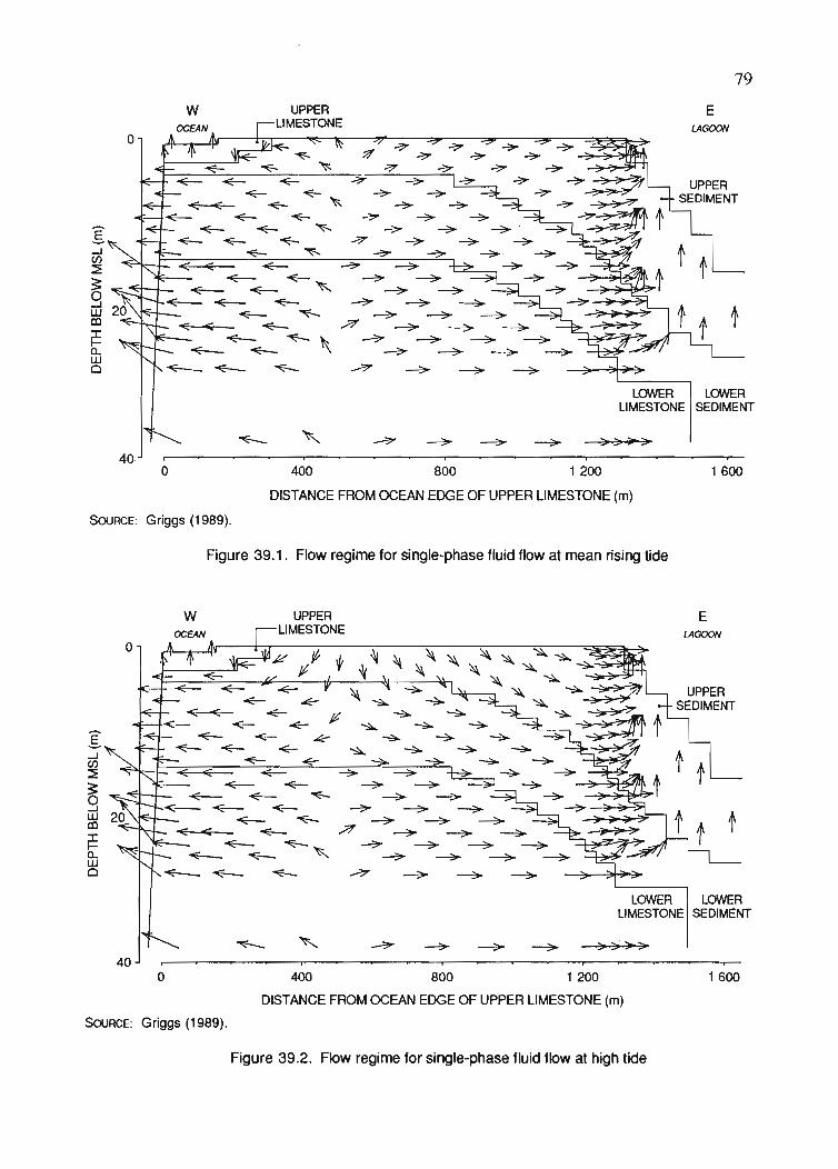
1 600
LOWER LOWERLIMESTONE SEDIMENT
»;;.->
1 200800400o
79
w ELAGOON
0~ ~;;f ~
~ '" "'7~ ~ ~ -?~
~"~
~ ~
~ ~ ~
~ ~ ~
t~ ~
t<: ~ -<:-- ~
t-<:-- -<:- '"~
~ -<:--~ -<:-- ~ ~
t t~ ~ ~
t~ /7~ ~ \ ~
-<:-- ~~~ ~ -"7
DISTANCE FROM OCEAN EDGE OF UPPER LIMESTONE (m)
SouRCE: Griggs (1989).
Figure 39.1. Flow regime for single-phase fluid flow at mean rising tide
UPPERLIMESTONE
E..J(f)
::E~
9wco~a.wCl
o
w
-<:---<:-- ~
~ -<:-- ~
~ -<:-- ~
~ ~
.... ~ -<:--~ ~"""
-<:-- ~ '"~~ ~
~
-->-->- -->-
~ ->- ->--:# ~ -->- -->-
/F ~ -->- -->-~ -->- -->- ->-~ -->- ->- ->-
->- -->- -->-
ELAGOON
LOWER LOWERLIMESTONE SEDIMENT
40o 400 800 1200
DISTANCE FROM OCEAN EDGE OF UPPER LIMESTONE (m)
1600
SouRCE: Griggs (1989).
Figure 39.2. Flow regime for single-phase fluid flow at high tide
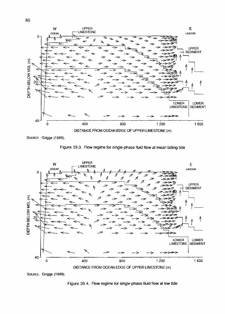
1600400 ·800 1 200
DISTANCE FROM OCEAN EDGE OF UPPER LIMESTONE (m)
o
80
w ELAGOON
0~
~
~
< -<--~ ~
I ~ ~
~...J
~ t(f)
t:::Et~
~
9UJ t tco t~11.UJCl ...-:',;J'
LQlNER LQlNERLIMESTONE SEDIMENT
~,
~ ~ ~ ~ »;'-)0
SouRCE: Griggs (1989).
Figure 39.3. Flow regime for single-phase fluid flow at mean falling tide
LOWER LQlNERLIMESTONE SEDIMENT
o
40o
w
~
~ ~
~ ~ ~
"""'~ ......->- ~/" ~ ......->- ~-=>-~~~
~......->-~--;..
~ ......->- --;..
i
400 800 1200
DISTANCE FROM OCEAN EDGE OF UPPER LIMESTONE (m)
ELAGOON
i
1600
SouRCE: Griggs (1989).
Figure 39.4. Flow regime for single-phase fluid flow at low tide
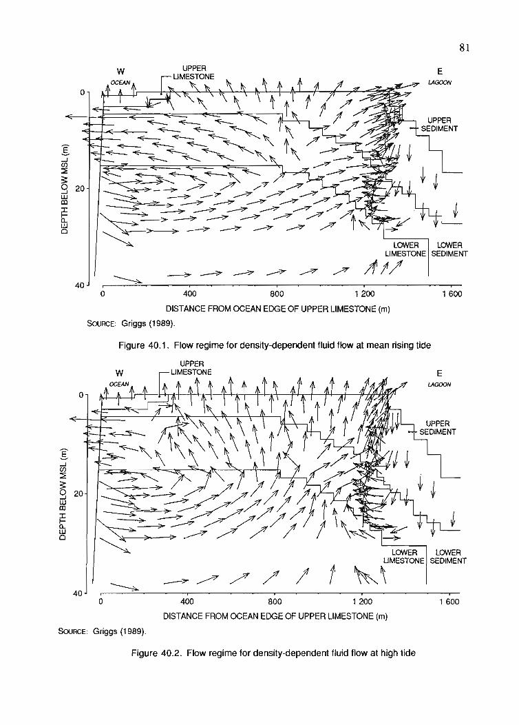
81
LOWER LOWERLIMESTONE SEDIMENT
AI/'i
1600
Ew
i' ,
o 400 800 1 200
DISTANCE FROM OCEAN EDGE OF UPPER LIMESTONE (m)
SOURCE: Griggs (1989).
g-'~
~ 20wco~0Wo
40
o
Figure 40.1. Flow regime for density-dependent fluid flow at mean rising tide
LOWER LOWERUMESTONE SEDIMENT
t ~\i
1600i i
400 800 1200
DISTANCE FROM OCEAN EDGE OF UPPER LIMESTONE (m)
o
o
40
g-'(J)
~
~ 20wco~0Wo
SouRCE: Griggs (1989).
Figure 40.2. Flow regime for density-dependent fluid flow at high tide

82
ELAGOON
~~~--<--~ /40 1'"",-~----""'i-~-~-~---r,---":;:::::"'------.-,-~-----r--i
o 400 800 1 200 1 600
DISTANCE FROM OCEAN EDGE OF UPPER LIMESTONE (m)
w
a
:[...J
~ ~~;J=~===:==:::::::~=~~==~~==l._..;;;;:9 ~"""""IoE--wco~ .I-.-
WCl
SouRCE: Griggs (1989).
Figure 40.3. Flow regime for density-dependent fluid flow at mean falling tide
o
w ELAGOON
LOWER LOWERUMESTONE SEDIMENT
40 ,....,---~--~=-"i--?~/-----'#~/_""" ....,J,?rr-/_--IJ_--.-:\-'!:l:r~-"~.....~--~--"r--o 400 800 t 1 200 1 600
DISTANCE FROM OCEAN EDGE OF UPPER LIMESTONE (m)
SouRCE: Griggs (1989).
Figure 40.4. Flow regime for density-dependent fluid flow at low tide
83
development involved simplifying assumptions. The two equations represent inexact
approximations of a physical problem. Determining the effect that simplifying assumptions
such as Darcy's law accurately describes fluid flow or that Fickian dispersion realistically
approximates macroscopic dispersion-had on this study is beyond the scope of the present
investigation. Nevertheless, it must be kept in mind that these assumptions influenced the
results.
Error also entered the results through the solution method. The finite-element method
consists of an approximate numerical solution rather than exact analytical solution. Truncation
of the Taylor series representing the derivatives in the governing equations introduced error that
caused unstable solutions when the time-step or nodal spacing became too large for the given
problem. The choice of proper element size and time-step length, however, provided stable
solutions. Additional error results from projecting variable values into the future to solve the
governing equations. The projection procedure includes the utilization of known information
and the assumption that the future rate of change of variables is equal to the past rate of change.
The use of small time-steps effectively eliminates this source of error.
The accuracy of assumptions employed in the approximation of the islet affected simulation
results. Assumptions encompassing boundary conditions, formation boundaries, permeability
contrast, formation-independent dispersivities, element size, and use of a two-dimensional
model introduced uncertainties that were difficult to assign to the simulations performed in this
study. More easily identifiable effects resulted from assumptions used in calibration of the
model. This discussion focuses on the influences that field-data quality, calibrated permeability
values, and calibrated dispersivity values had on simulation results.
Comparison of the pumping simulations that used mesh 3 with the equivalent simulations
that employed mesh 4 revealed the dependence of the solution on the calibrated parameter
values. Errors in the calibrated permeability and dispersivity values may have significantly
affected conclusions based on the results of simulations that used the erroneous parameters.
The accuracy of the calibrated permeability and dispersivity values depended on the quality and
compatibility of the recharge and salinity data. Recharge directly affected the size of the lens.
Overestimated recharge rates would have resulted in high calibrated permeabilities and low
calibrated dispersivities. In terms of pumping, the consequence of this scenario would have
been reduced upconing, causing an overestimation of the maximum allowable withdrawal rate.
The opposite would have resulted from underestimated recharge rates.
The equilibrium between the calculated recharge rate and the measured salinity influenced
the conclusions in a similar manner. Salinity measurements made throughout the duration of
the study of Hamlin and Anthony (1987) indicated freshwater lens growth. Thus, the lens
existed in a state of disequilibrium with the recharge rate, and the measured lens was too small
84
for the measured rainfall rate. This suggests that if the recharge rate used were accurate, the
calibration would have produced results similar to those produced in the case of an
overestimated recharge rate. Calibrated permeabilities would have been too large to reduce the
lens size, and the high penneability would have required low dispersivities to offset the higher
fluid velocity. However, the larger lens, which would result in the field when the lens reached
equilibrium with the measured recharge rate, would have allowed a greater pumping rate. The
dominating effect remains unclear without more data and further simulation.
The accuracy of the field salinity measurements directly affected calibration of the model.
Overestimation of the depth of the 50% isochlor and the thickness of the transition zone would
have resulted in error similar to that resulting from an underestimated recharge rate. This would
have produced low calibrated penneabilities and high calibrated dispersivities. Underestimation
of the depth of the 50% salinity contour and the thickness of the transition zone would have
had the opposite effect. The consequences of overestimating the depth of the 50% isochlor and
underestimating the thickness of the transition zone, or underestimating the depth of the 50%
isochlor and overestimating the thickness of the transition zone, were difficult to determine
with the simulations perfonned in this study.
The inability to calibrate SUTRA with tides is another potential source of error. The
dispersion model in SUTRA was used in this study to simulate the mixing of fresh water and
seawater caused by tides in the field. The dispersion model adequately reproduced the amount
of mixing observed in the field for an undeveloped lens. However, pumping changes the flow
regime and the amount of mixing. It remains uncertain whether or not the dispersion model can
accurately reproduce the mixing caused by the combination of tides and pumping. In other
words, the calibrated parameters may be in error to account for the absence of tides. In this
case, the response of the lens to pumping would also be in error. Without being able to
simulate tides, the effect on the conclusions of this study is unclear.
CONCLUSIONS AND FUTURE RESEARCH
The numerical model SUTRA, which solves two-dimensional density-dependent fluid flow and
solute-transport equations, was used to simulate groundwater flow with solute transport for the
Laura area of Majuro Atoll, Marshall Islands. The conclusions from this work encompass both
freshwater lens development and management aspects as well as technical aspects of the
mathematical model and small-island hydraulics. The conclusions in this section must be
qualified by the understanding that discretization of the simulated region and estimation of the
parameters produced only an approximation of Laura. It must be cautioned that these

85
conclusions must be interpreted within the assumptions invoked to approximate Laura and
allow numerical simulation of a three-dimensional entity in two dimensions.
Technical Conclusions
Conclusions for technical aspects of SUlRA and small-island hydraulics include:
1. For calibration of the model, permeability controlled the depth of the center of the
transition zone for a fixed recharge rate, and the transverse dispersivity had the greatest
effect on the transition-zone thickness.
2. As shown by the sensitivity analysis, the results of simulations strongly depend on the
calibrated parameter values. The accuracy of the calibrated parameter values depends
on the quality of the recharge and salinity field data.
3. Density-dependent fluid flow greatly affected the groundwater flow regime and must
be included in projects concerned with the study of the flow dynamics of atolls and
small islands.
4. The use of AMR values demonstrated that the simulated lens responded to changes in
recharge after approximately one month.
5. Higher MSL in the lagoon, of the magnitude employed in this study, raised the salinity
of water in the lower limestone, yet increased the thickness of the transition zone and
failed to cause the truncation of the base of the transition zone at the lower sediment
lower limestone boundary.
Managerial Conclusions
Recommendations for freshwater lens development and management for Laura include:
1. Infiltration galleries produce less upconing than conventional vertical wells and
represent the most efficient well type for maximizing pumping rates. To minimize
upconing, infiltration galleries should be installed near the water table in the central
portion of the islet, not necessarily above the deepest portion of the lens.
2. Pumping simulations indicate Laura can supply between 1.4 million and 2.1 million I
of fresh water per day under the recharge rates measured by Hamlin and Anthony
(1987), although the maximum allowable pumping rate for a gallery is undeterminable
using a two-dimensional model.
3. During severe droughts, Laura can provide significant quantities of fresh water or
low-salinity water, which would be easier to desalinize than seawater.
4. Seawater washover from large storms may halt pumping for up to six months if no
remedial pumping is employed.
86
5. Installation of a grout wall to a depth of 15.2 m on the ocean side of the islet produced
little increase in the storage of fresh water within the lens and appears uneconomical,
although pumping with the wall in place was not simulated.
The consequence of being unable to predict the maximum allowable pumping rate from a
gallery, as stated above, requires that initial field pumping rates be values well below the
maximum rates predicted in this investigation. Continuous monitoring of the upconing
produced by pumping will be necessary to determine the accuracy of predictions made by this
project. Areally extensive galleries with several pumps will most closely match these
predictions.
Future Research
The following discussion covers several proposals for future research projects on atolls. The
suggestions apply to Laura as well as to atolls in general.
Additional simulations need to be perfonned to further evaluate pumping with seawater
washover and the effects of a grout wall. These simulations should begin with the final
solutions of the corresponding simulations presented in the section on results. Continuation of
the simulations begun in this study would provide a simple and rapid first approximation of the
worth of remedial pumping to aid in lens recovery from seawater washover and of the potential
for increasing pumping rates in Laura with a grout wall constructed near the ocean.
With the exception of the above simulations or simple simulations concerning general
aspects of atoll hydraulics or basic management options, work should progress toward a more
comprehensive modeling approach and approximation of the atoll. Both of these suggestions
require more data than were available for the present study. A more comprehensive modeling
approach requires the collection of data over time. At least one, and preferably more, validation
data sets are needed to strengthen the modeling approach employed in this study. The approach
should include validating the calibrated model instead of assuming the calibration is valid.
Upconing data from the developed lens would serve both as a check on the accuracy of the
predictions made in this study and as a validation data set with which to recalibrate the model if
necessary. A data set from the developed lens would be useful because it would include the
effects of changes in the flow regime resulting from the addition of pumping. Parameters
calibrated using data sets that exclude the effects of pumping may become invalid upon the
initiation of pumping because the flow regime will change.
A more comprehensive approximation of the atoll requires collection of data from more
than the three boreholes used in this study. Numerous deep boreholes are needed to define the
geology of the entire islet. This would enable better approximation of several cross sections for

87
two-dimensional analysis or better approximation of the islet as a whole for three-dimensional
analysis. In conjunction with the need for additional geologic data is the need for high-quality
hydrogeologic data. These data should consist of penneability and porosity measurements to
better defme the aquifer, and salinity and recharge infonnation to better define the lens and
water balance.
Modeling of Laura can also be improved by employing a faster computer with larger
memory so that the mesh can be refined to give better resolution of parameter variations and
concentration profiles. Finer discretization of the mesh would increase the possibility of
including tides because the smaller element size would allow smaller dispersivities, which
would reduce the amount of mixing calculated by the model. Tides and AMR rates must be used
to make boundary conditions for Laura as accurate as possible.
A more accurate penneability distribution would require a relaxation of the constraints
placed on penneabilities in this study. Results from this study suggest that permeability
increases laterally in the direction from the lagoon to the ocean. This is supported in the field by
the visible increase in grain size observed for the upper sediment layer. Furthermore, the
inability to calibrate the model with tides indicated the possibility that anisotropic permeabilities
are needed.
Ultimately, a three-dimensional density-dependent model should be used to simulate
pumping schemes. Quantities of extractable water are difficult to detennine with a two
dimensional model. Moreover, the assumption that parameters remain constant in the third
dimension is a severe limitation of two-dimensional analysis, and its effect needs to be
quantified.
In summary, future studies should focus attention on the following four tasks:
1. Performing additional first approximation simulations using the approach of this study
2. Collecting high-quality field data in time and space
3. Eliminating assumptions used in this study to more accurately approximate Laura for
two-dimensional analysis
4. Using a three-dimensional density-dependent model to simulate pumping schemes.
ACKNOWLEDGMENTS
We would like to acknowledge the University of Guam's Water and Energy Research Institute
of the Western Pacific and the Water Resources Research Center of the University of Hawaii at
Manoa for their fmancial support, which has made this study possible. We would especially
like to thank Keith Loague, of the University of California at Berkeley, for his assistance with
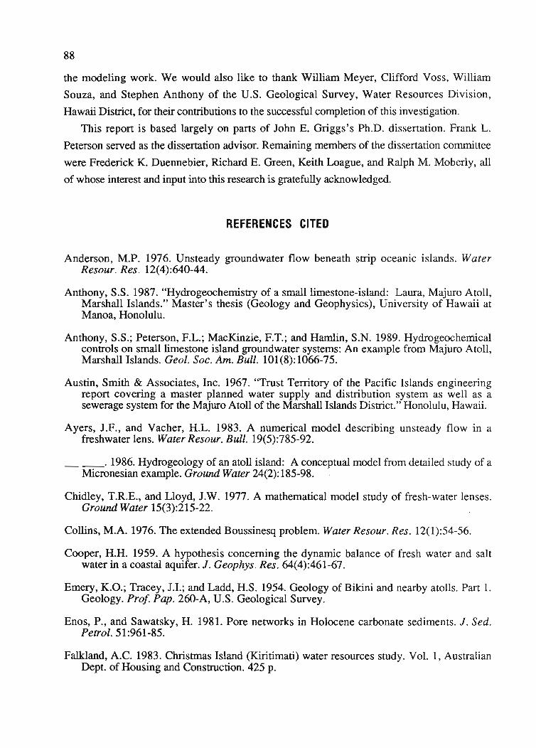
88
the modeling work. We would also like to thank William Meyer, Clifford Voss, William
Souza, and Stephen Anthony of the U.S. Geological Survey, Water Resources Division,
Hawaii District, for their contributions to the successful completion of this investigation.
This report is based largely on parts of John E. Griggs's Ph.D. dissertation. Frank L.
Peterson served as the dissertation advisor. Remaining members of the dissertation committee
were Frederick K. Duennebier, Richard E. Green, Keith Loague, and Ralph M. Moberly, all
of whose interest and input into this research is gratefully acknowledged.
REFERENCES CITED
Anderson, M.P. 1976. Unsteady groundwater flow beneath strip oceanic islands. WaterResour. Res. 12(4):640-44.
Anthony, S.S. 1987. "Hydrogeochemistry of a small limestone-island: Laura, Majuro Atoll,Marshall Islands." Master's thesis (Geology and Geophysics), University of Hawaii atManoa, Honolulu.
Anthony, S.S.; Peterson, FL.; MacKinzie, F.T.; and Hamlin, S.N. 1989. Hydrogeochemicalcontrols on small limestone island groundwater systems: An example from Majuro Atoll,Marshall Islands. Geol. Soc. Am. Bull. 101(8):1066-75.
Austin, Smith & Associates, Inc. 1967. "Trust Territory of the Pacific Islands engineeringreport covering a master planned water supply and distribution system as well as asewerage system for the Majuro Atoll of the Marshall Islands District." Honolulu, Hawaii.
Ayers, J.F., and Vacher, H.L. 1983. A numerical model describing unsteady flow in afreshwater lens. Water Resour. Bull. 19(5):785-92.
___.1986. Hydrogeology of an atoll island: A conceptual model from detailed study of aMicronesian example. Ground Water 24(2):185-98.
Chidley, T.R.E., and Lloyd, J.W. 1977. A mathematical model study of fresh-water lenses.Ground Water 15(3):215-22.
Collins, M.A. 1976. The extended Boussinesq problem. Water Resour. Res. 12(1):54-56.
Cooper, H.H. 1959. A hypothesis concerning the dynamic balance of fresh water and saltwater in a coastal aquifer. J. Geophys. Res. 64(4):461-67.
Emery, K.O.; Tracey, J.I.; and Ladd, H.S. 1954. Geology of Bikini and nearby atolls. Part 1.Geology. Prof Pap. 260-A, U.S. Geological Survey.
Enos, P., and Sawatsky, H. 1981. Pore networks in Holocene carbonate sediments. J. Sed.Petrol. 51:961-85.
Falkland, A.C. 1983. Christmas Island (Kiritimati) water resources study. Vol. 1, AustralianDept. of Housing and Construction. 425 p.
89Fetter, C.W. 1972. Position of the saline water interface beneath oceanic islands. WaterResour. Res. 8(5):1307-15.
Freeze, RA., and Cherry, J.A. 1979. Groundwater. Englewood, N.J.: Prentice Hall.
Gardner, A.O.; Peaceman, D.W.; and Pozzi, A.L., Jr. 1964. Numerical calculation ofmultidimensional miscible displacement by the method of characteristics. J. Soc. Petrol.Eng. 4(1):26-36.
Ghyben, W.B. 1888. Nota in verband met de voorgenomen putboring nabij Amsterdam.Tijdschrift van Let Koninklijk Inst. van Ing.
Glover, RE. 1959. The pattern of fresh water flow ,in a coastal aquifer. J. Geophys. Res.64(4):457-59.
Griggs, J.E. 1989. "Simulation of an optimal groundwater development scheme on the Lauraend of Majuro Atoll, Marshall Islands." Ph.D. dissertation (Geology and Geophysics),University of Hawaii at Manoa, Honolulu.
Hamlin, S.N., and Anthony, S.S. 1987. Ground-water resources of the Laura area, MajuroAtoll, Marshall Islands. Water Resour. Inves. Rep. 87-4047, U.S. Geological Survey.Hantush, M.S. 1968. Unsteady movement of fresh water in thick unconfined saline aquifers.Bull. Int. Assoc. Sci. Hydrol. 13:40-60.
Henry, H.R. 1964. Effects of dispersion on salt encroachment in coastal aquifers. WaterSupply Pap. 1613C: C70-C84. U.S. Geological Survey.
Herman, M.E. 1984. "Tidal fluctuations and ground-water dynamics in atoll island aquifers."Master's thesis, University of Nevada-Reno, Reno, Nevada.
Herman, M.E.; Buddemier, R.W.; and Wheatcraft, S.W. 1986. A layered aquifer model ofatoll island hydrology: Validation of a computer simulation. J. Hydrol. 84:303-322.
Herzberg, A. 1901. Die Wasserversorgung einiger Nordseebader. 1. Gasbeleucht.Wasserversorg.44:815-19.
Hogan, P. 1988. "Modeling of freshwater-seawater interaction on Enjebi Island, EnewetakAtoll." Master's thesis, San Jose State University, California. 75 p.
Hubbert, M.K. 1940. The theory of ground-water motion. 1. Geol. Res. 48:785-944.
Hunt, C.D., Jr., and Peterson, P.L. 1980. Groundwater resources of Kwajalein Island,Marshall Islands. Tech. Rep. No. 126, Water Resources Research Center, University ofHawaii at Manoa, Honolulu. 91 p.
Johnson, G. 1986. Everywhere education level rises, birth rates comes down. Marshall IslandNewspaper 17(42):14.
Lam, RK. 1974. Atoll permeability calculated from tidal diffusion. J. Geophys. Res.79(21):3073-81.
Lee, c., and Cheng, RT. 1974. On seawater encroachment in coastal aquifers. Water Resour.Res. 10(5):1039-43.
90Lloyd, J.W.; Miles, J.e.; Chessman, G.R.; and Bugg, S.F. 1980. A groundwater resources
study of a Pacific Ocean atoll-Tarawa, Gilbert Islands. Water Resour. Bull. 16(4):646-53.
M&E Pacific, Inc., and Juan C. Tenorio & Associates, Inc. 1979. Wastewater facilities plan,Marshall District Volume 1-Darrit-Uliga-Dalap and Laura Islands, Section II.
Masch, F.D., and Denny, K.J. 1966. Grain-size distribution and its effects on the penneabilityof unconsolidated sands. Water Resour. Res. 2:665-77.
Peaceman, D.W., and Rachford, H.H., Jr. 1955. The numerical solution of parabolic andelliptic differential equations. J. Soc. Ind. Appl. Math. 3:28-41.
Pinder, G.F., and Cooper, H.H., Jr. 1970. A numerical technique for calculating the transientposition of the saltwater front. Water Resour. Res. 6(3):875-82.
Pinder, G.F., and Gray, W.G. 1977. Finite element simulation in surface and subsurfacehydrology. New York:: Academic.
Reddell, D.L., and Sunada, D.K. 1970. Numerical simulation of dispersion in groundwateraquifers. Hydrol. Pap. No. 41, Colorado State University, Fort Collins, Colorado. 79 p.
Remson, I.; Hornberger, G.M.; and Molz, F.J. 1971. Numerical methods in subsurfacehydrology. New York: Wiley-Interscience.
Reynolds, W.D.; Elrick, D.E.; and Clothier, RE. 1985. The constant head well pennearneter:Effect of unsaturated flow. Soil Sci. 139(2):172-80.
Rumer, R.R., and Shiau, J.e. 1968. Salt water interface in a layered coastal aquifer. WaterResour. Res. 4(6):1235-47.
Sa da Costa, A.A., and Wilson, J.L. 1979. "A numerical model of seawater intrusion inaquifers." Rep. No. 247, Department of Civil Engineering, Massachusetts Institute ofTechnology.
Schlanger, S.O. 1963. Subsurface geology of Enewetak Atoll. Prof Pap. 260-BB, u.S.Geological Survey.
Segol, G., and Pinder, G.F. 1976. Transient simulation of saltwater intrusion in southeasternFlorida. Water Resour. Res. 12(1):65-70.
Segol, G.; Pinder, G.F.; and Gray, W.G. 1975. A Galerkin-finite element technique forcalculating the transient position of the saltwater front. Water Resour. Res. 11(2):343-47.
Swartz, J.H. 1962. Some physical constants for the Marshall Islands area. Prof Pap. 260AA, pp. 953-990. U.S. Geological Survey.
U.S. National Oceanic and Atmospheric Administration. 1984. Climatological data, annualsummary, Hawaii and Pacific area, vol. 80, no. 13.40 p.
___-. 1985. Local climatological data, annual summary with comparative data, Majuro,Marshall Islands. 8 p.
Vacher, H.L. 1974. Groundwater hydrology of Bennuda. Government of Bennuda, PublicWorks Department, Hamilton, Bennuda. 87 p.
91
Van der Veer, P. 1977. Analytical solution for steady interface flow in a coastal aquiferinvolving a phreatic surface with precipitation. J. Hydrol. 34:1-11.
Voss, C. 1984. A finite-element simulation model for saturated-unsaturated, fluid-densitydependent ground-water flow with energy transport of chemically-reactive single-speciessolute transport. Water-Resour. Investigation Rep. 84-4369, U.S. Geological Survey.
Voss, C., and Souza, W.R 1987. Variable density flow and solute transport simulation ofregional aquifers containing a narrow freshwater-saltwater transition zone. Water Resour.Res. 23(10):1851-66.
Weast, RC., and Astle, M.J. 1980. CRC handbook of chemistry and physics. Boca Raton,Fla.: CRC Press.
Wheatcraft, S.W., and Buddemeier, RW. 1981. Atoll island hydrology. Ground Water19(3):311-20.