Lecture Notes in Geoinformation and Cartography

Remote Sensing and Geospatial Technologies for Coastal EcosystemAssessment and Management

Bearbeitet vonXiaojun Yang

1. Auflage 2009. Buch. xiv, 561 S. HardcoverISBN 978 3 540 88182 7

Format (B x L): 15,5 x 23,5 cmGewicht: 1122 g

Weitere Fachgebiete > Geologie, Geographie, Klima, Umwelt > Geologie undNachbarwissenschaften > Paläontologie, Taphonomie

Zu Inhaltsverzeichnis

schnell und portofrei erhältlich bei

Die Online-Fachbuchhandlung beck-shop.de ist spezialisiert auf Fachbücher, insbesondere Recht, Steuern und Wirtschaft.Im Sortiment finden Sie alle Medien (Bücher, Zeitschriften, CDs, eBooks, etc.) aller Verlage. Ergänzt wird das Programmdurch Services wie Neuerscheinungsdienst oder Zusammenstellungen von Büchern zu Sonderpreisen. Der Shop führt mehr

als 8 Millionen Produkte.

Chapter 2Sensors and Techniques for ObservingCoastal Ecosystems

Victor V. Klemas

This chapter reviews the advances in sensor design and related field techniques thatare particularly appropriate for coastal ecosystem research and management. Multi-spectral and hyperspectral imagers are available for mapping coastal land cover andconcentrations of organic or inorganic suspended particles and dissolved substancesin coastal waters. Thermal infrared scanners can map sea surface temperatures accu-rately and chart coastal currents, while microwave radiometers can measure oceansalinity, soil moisture and other hydrologic parameters. Radar imagers, scatterom-eters and altimeters provide information on ocean waves, ocean winds, sea surfaceheight and coastal currents. Using airborne LIDAR one can produce bathymetricmaps, even in moderately turbid coastal waters. Since coastal ecosystems have highspatial complexity and temporal variability, they frequently have to be observedfrom both, satellites and aircraft, in order to obtain the required spatial, spectral andtemporal resolutions. A reliable field data collection approach using ships, buoys,and field instruments with a valid sampling scheme is required to calibrate andvalidate the remotely sensed information.

2.1 Introduction

To understand and manage ecosystems, one must monitor and study their biologi-cal/physical features and controlling processes. However, obtaining this informationfor coastal ecosystems is quite challenging since they exhibit extreme variations inspatial complexity and temporal variability. Also, the influence of coastal ecosys-tems extends well beyond the local scale, and the only realistic means of obtainingdata over such large areas is by remote sensing. To accomplish such monitoringaccurately and cost-effectively, the design of the monitoring approach must makeintegrated use of remote sensing and field techniques (Kerr and Ostrovsky 2003).

V.V. Klemas (B)College of Marine and Earth Studies, University of Delaware, Newark, DE 19716, USAe-mail: klemas@udel.edu

X. Yang (ed.), Remote Sensing and Geospatial Technologies for Coastal Ecosystem 17Assessment and Management, Lecture Notes in Geoinformation and Cartography,DOI 10.1007/978-3-540-88183-4 2, c© Springer-Verlag Berlin Heidelberg 2009

18 V.V. Klemas

Advances in technology and decreases in cost are now making remote sensing(RS) and geographic information systems (GIS) practical and attractive for use incoastal ecosystem management. They are also allowing researchers and managersto take a broader view of ecological patterns and processes. Landscape-level envi-ronmental indicators that can be detected by remote sensors are available to providequantitative estimates of coastal and estuarine habitat conditions and trends. Suchindicators include watershed land cover, riparian buffers, wetland losses and frag-mentation, marsh productivity, invasive species, beach erosion, water turbidity andchlorophyll concentrations, among others. New satellites, carrying sensors with finespatial (1–4 m) and spectral (200 narrow bands) resolutions are being launched, pro-viding a capability to more accurately detect changes in coastal habitat and wetlandhealth. Advances in the application of GIS help incorporate ancillary data layers toimprove the accuracy of satellite land-cover classification. When these techniquesfor generating, organizing, storing, and analyzing spatial information are combinedwith watershed and ecosystem models, coastal planners and managers have a meansfor assessing the impacts of alternative management practices.

In Sects. 2.2 and 2.3 of this chapter, the reader is introduced to those airborneand spaceborne remote sensors and techniques which are cost-effective for studyingand monitoring coastal ecosystems. In Sects. 2.4 and 2.5, case studies are used toillustrate the application of selected remote sensors and techniques to monitor en-vironmental indicators related to coastal wetland health and estuarine water quality.Section 2.6 describes the most important field techniques required for coastal re-mote sensing projects. Section 2.7 summarizes the main points followed by a list ofcarefully selected references.

2.2 Remote Sensors

Aerial photography started approximately in 1858 when the famous French photog-rapher, Gaspard Tournachon, obtained the first aerial photographs from a balloonnear Paris. Since then, aerial photography has advanced, primarily during war times,to include color infrared films (for camouflage detection) and sophisticated cameras.Aerial photography and other remote sensing techniques are now used successfullyin agriculture, forestry, land use planning, fire detection, mapping wetlands andbeach erosion, oceanography and many other applications. For instance, in agri-culture they have been used for land-use inventories, soil surveys, crop conditionestimates, yield forecasts, acreage estimates, crop insect/pest/disease detection, irri-gation management, and more recently, precision agriculture (Jensen 2007).

A major advance in aerial remote sensing has been the development of digitalaerial cameras (Al-Tahir et al. 2006). Digital photography is capable of deliver-ing photogrammetric accuracy and coverage as well as multispectral data at anyuser-defined resolution down to 0.1 m ground sampling distance. It provides pho-togrammetric positional accuracy with multispectral capabilities for image analy-sis and interpretation. As no chemical film processing is needed, the direct digital

2 Sensors and Techniques for Observing Coastal Ecosystems 19

acquisition can provide image data in just a few hours compared to several weeksusing the traditional film-based camera. Another advantage over the traditional filmis the ability to assess the quality of data taken directly after the flight is completed.Two examples of digital mapping cameras, ADS40 by Leica Geosystems and DMCfrom Z/I Imaging, were first presented to the market in 2002 to address require-ments for extensive coverage, high geometric and radiometric resolution and accu-racy, multispectral imagery, and stereo capability (Leica 2002).

Since the 1960s, remote sensing has progressed to include new techniques ofinformation collection that include aircraft and satellite platforms carrying electro-optical and antenna sensor systems (Campbell 2007). Up to that time, camera sys-tems dominated image collection, and photographic media dominated the storageof the spatially varying visible (VIS) and near-infrared (NIR) radiation intensitiesreflected from the Earth. Beginning in the 1960s, electronic sensor systems wereincreasingly used for collection and storage of the Earth’s reflected radiation, andsatellites were developed as an alternative to aircraft platforms.

Advances in electronic sensors and satellite platforms were accompanied by anincreased interest and use of electromagnetic radiant energy not only from the VISand NIR wavelength regions, but also from the thermal infrared (TIR) and mi-crowave regions. For instance, TIR is used for mapping sea surface temperature andmicrowaves (e.g. radar) are used for measuring sea surface height, currents, wavesand winds on a global scale (Martin 2004).

While most geologists, geographers, and other earth scientists are familiar withaerial photography techniques (Sabins 1978, Avery and Berlin 1992), relatively fewscientists have had the opportunity to use thermal infrared, radar, and LIDAR data.Since the TIR radiance depends on both the temperature and emissivity of the target,it is difficult to measure land surface temperatures, because the emissivity will varyas the land cover changes. On the other hand, over water the emissivity is knownand nearly constant, 98%, approaching the behavior of a perfect blackbody radiator(Ikeda and Dobson 1995). Thus the TIR radiance measured over the oceans willvary primarily with the sea surface temperature (SST) and allow one to determinethe SST accurately (±0.5◦C), with some atmospheric corrections (Martin 2004,Elachi and van Ziel 2006).

Radar images represent landscape and ocean surface features that differ signifi-cantly from those observed by aerial photography or multispectral scanners. A Side-looking Airborne Radar (SLAR) irradiates a swath along the aircraft flight directionby scanning the terrain with radar pulses at right angles to the flight path. Thusthe radar image is created by pulse energy reflected from the terrain and representsprimarily surface topography. Since radar images look quite different from visiblephotographs, they require specialized interpretation skills. Radar pulses penetrateonly a few wavelengths into the soil, depending on soil moisture, salinity, surfaceroughness, etc. The range resolution of SLAR depends on the length of the radarpulse which can be made quite short with new electronic techniques. However, theazimuth resolution is limited by the antenna size and altitude, thus preventing SLARsystems to be used on satellites.

20 V.V. Klemas

Synthetic Aperture Radar (SAR) was specifically developed to provide high res-olution images from satellite altitudes. SAR employs the Doppler shift technique tonarrow down the azimuth resolution even with a small antenna. Thus range and az-imuth resolutions of the order of 10 m are obtainable with SAR mounted on satelliteplatforms (Radarsat, ERS-2). In oceanography, radar is used not only for imagingthe sea surface but also as altimeters to map sea surface height; scatterometers to de-termine sea surface winds; etc. (Ikeda and Dobson 1995, Martin 2004). Radar canpenetrate fog and clouds, making it particularly valuable for emergency applicationsand in areas where cloud cover persists. Passive microwave radiometers are becom-ing important for measuring sea surface salinity, soil moisture and a wide range ofhydrology related parameters (Burrage et al. 2003, Parkinson 2003).

Airborne LIDAR (Light Detection and Ranging) has become quite useful fortopographic and bathymetric mapping. Laser profilers are unique in that they confinethe coherent light energy in a very narrow beam, providing pulses of very high peakintensity. This enables LIDARS to penetrate moderately turbid coastal waters forbathymetric measurements or gaps in forest canopies to provide topographic datafor digital elevation models (Brock and Sallenger 2000). The water depth is derivedby comparing the travel times of the LIDAR pulses reflected from the sea bottomand the water surface.

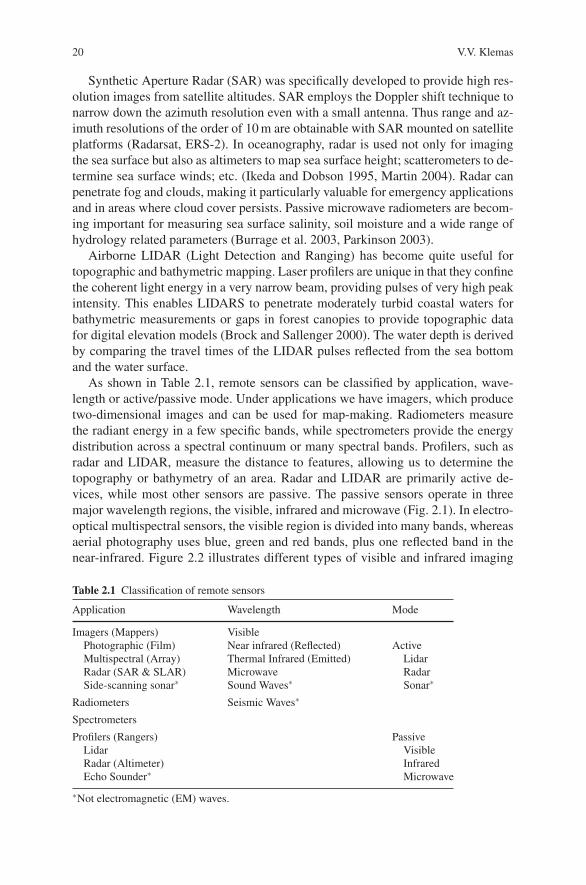
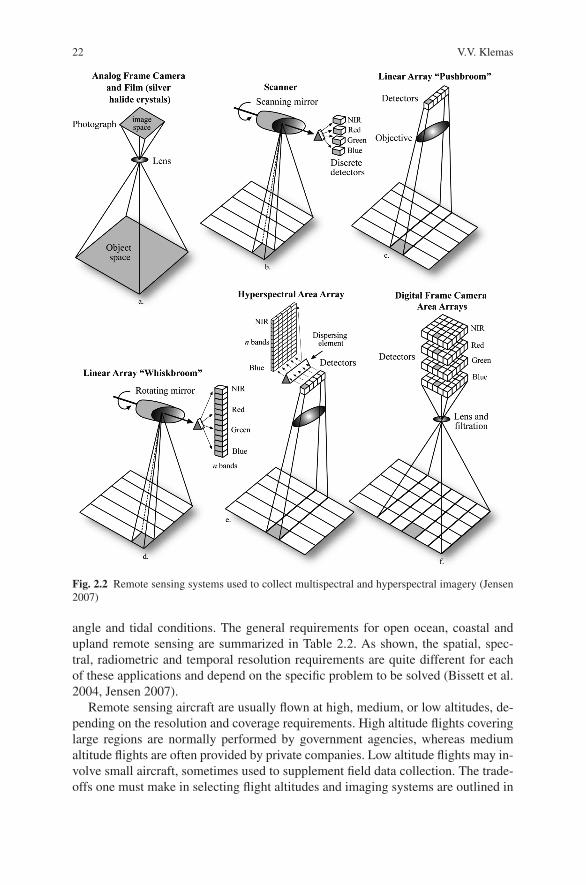
As shown in Table 2.1, remote sensors can be classified by application, wave-length or active/passive mode. Under applications we have imagers, which producetwo-dimensional images and can be used for map-making. Radiometers measurethe radiant energy in a few specific bands, while spectrometers provide the energydistribution across a spectral continuum or many spectral bands. Profilers, such asradar and LIDAR, measure the distance to features, allowing us to determine thetopography or bathymetry of an area. Radar and LIDAR are primarily active de-vices, while most other sensors are passive. The passive sensors operate in threemajor wavelength regions, the visible, infrared and microwave (Fig. 2.1). In electro-optical multispectral sensors, the visible region is divided into many bands, whereasaerial photography uses blue, green and red bands, plus one reflected band in thenear-infrared. Figure 2.2 illustrates different types of visible and infrared imaging

Table 2.1 Classification of remote sensors

Application Wavelength Mode

Imagers (Mappers) VisiblePhotographic (Film) Near infrared (Reflected) ActiveMultispectral (Array) Thermal Infrared (Emitted) LidarRadar (SAR & SLAR) Microwave RadarSide-scanning sonar∗ Sound Waves∗ Sonar∗

Radiometers Seismic Waves∗

Spectrometers

Profilers (Rangers) PassiveLidar VisibleRadar (Altimeter) InfraredEcho Sounder∗ Microwave

∗Not electromagnetic (EM) waves.

2 Sensors and Techniques for Observing Coastal Ecosystems 21

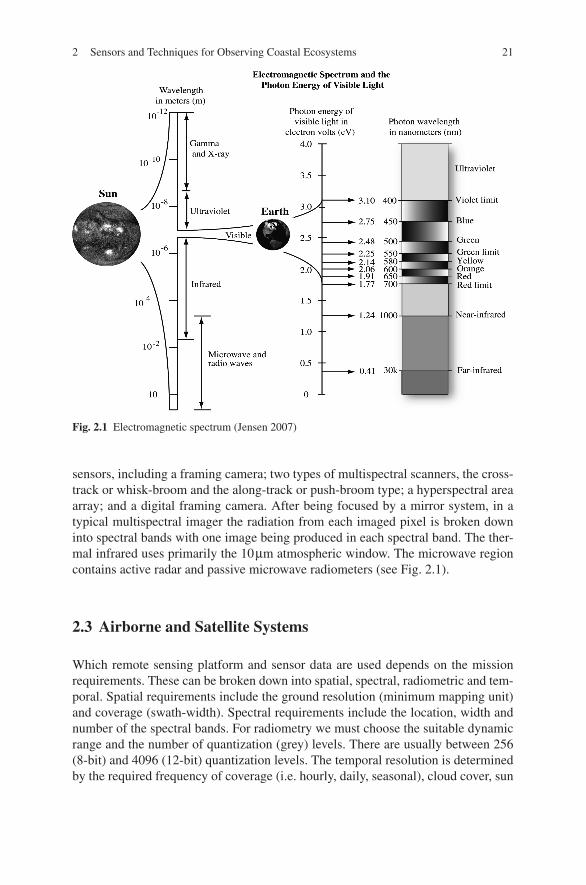
Fig. 2.1 Electromagnetic spectrum (Jensen 2007)

sensors, including a framing camera; two types of multispectral scanners, the cross-track or whisk-broom and the along-track or push-broom type; a hyperspectral areaarray; and a digital framing camera. After being focused by a mirror system, in atypical multispectral imager the radiation from each imaged pixel is broken downinto spectral bands with one image being produced in each spectral band. The ther-mal infrared uses primarily the 10μm atmospheric window. The microwave regioncontains active radar and passive microwave radiometers (see Fig. 2.1).

2.3 Airborne and Satellite Systems

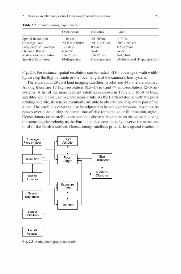
Which remote sensing platform and sensor data are used depends on the missionrequirements. These can be broken down into spatial, spectral, radiometric and tem-poral. Spatial requirements include the ground resolution (minimum mapping unit)and coverage (swath-width). Spectral requirements include the location, width andnumber of the spectral bands. For radiometry we must choose the suitable dynamicrange and the number of quantization (grey) levels. There are usually between 256(8-bit) and 4096 (12-bit) quantization levels. The temporal resolution is determinedby the required frequency of coverage (i.e. hourly, daily, seasonal), cloud cover, sun

22 V.V. Klemas

Fig. 2.2 Remote sensing systems used to collect multispectral and hyperspectral imagery (Jensen2007)

angle and tidal conditions. The general requirements for open ocean, coastal andupland remote sensing are summarized in Table 2.2. As shown, the spatial, spec-tral, radiometric and temporal resolution requirements are quite different for eachof these applications and depend on the specific problem to be solved (Bissett et al.2004, Jensen 2007).

Remote sensing aircraft are usually flown at high, medium, or low altitudes, de-pending on the resolution and coverage requirements. High altitude flights coveringlarge regions are normally performed by government agencies, whereas mediumaltitude flights are often provided by private companies. Low altitude flights may in-volve small aircraft, sometimes used to supplement field data collection. The trade-offs one must make in selecting flight altitudes and imaging systems are outlined in

2 Sensors and Techniques for Observing Coastal Ecosystems 23

Table 2.2 Remote sensing requirements

Open ocean Estuaries Land

Spatial Resolution 1–10 km 20–200 m 1–30 mCoverage Area 2000×2000km 200×200km 200×200kmFrequency of Coverage 1–6 days 0.5–6 h 0.5–5 yearsDynamic Range Narrow Wide WideRadiometric Resolution 10–12 bits 10–12 bits 8–10 bitsSpectral Resolution Multispectral Hyperspectral Multispectral (Hyperspectral)

Fig. 2.3. For instance, spatial resolution can be traded off for coverage (swath width)by varying the flight altitude or the focal length of the camera’s lens system.

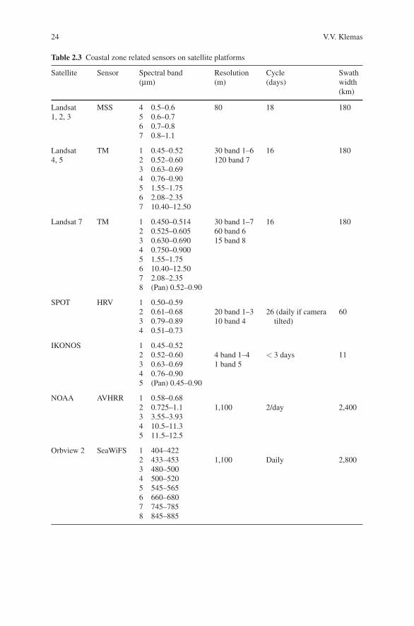
There are about 29 civil land imaging satellites in orbit and 34 more are planned.Among these are 18 high-resolution (0.5–1.8 m) and 44 mid-resolution (2–36 m)systems. A list of the more relevant satellites is shown in Table 2.3. Most of thesesatellites are in polar, sun-synchronous orbits. As the Earth rotates beneath the polarorbiting satellite, its sensors eventually are able to observe and map every part of theglobe. The satellite’s orbit can also be adjusted to be sun-synchronous, repeating itspasses over a site during the same time of day (or same solar illumination angle).Geostationary orbit satellites are stationed above a fixed point on the equator, havingthe same angular velocity as the Earth, and thus continuously observe the same onethird of the Earth’s surface. Geostationary satellites provide less spatial resolution

Fig. 2.3 Aerial photography trade-offs

24 V.V. Klemas

Table 2.3 Coastal zone related sensors on satellite platforms

Satellite Sensor Spectral band(μm)

Resolution(m)

Cycle(days)

Swathwidth(km)

Landsat MSS 4 0.5–0.6 80 18 1801, 2, 3 5 0.6–0.7

6 0.7–0.87 0.8–1.1

Landsat TM 1 0.45–0.52 30 band 1–6 16 1804, 5 2 0.52–0.60 120 band 7

3 0.63–0.694 0.76–0.905 1.55–1.756 2.08–2.357 10.40–12.50

Landsat 7 TM 1 0.450–0.514 30 band 1–7 16 1802 0.525–0.605 60 band 63 0.630–0.690 15 band 84 0.750–0.9005 1.55–1.756 10.40–12.507 2.08–2.358 (Pan) 0.52–0.90

SPOT HRV 1 0.50–0.592 0.61–0.68 20 band 1–3 26 (daily if camera 603 0.79–0.89 10 band 4 tilted)4 0.51–0.73

IKONOS 1 0.45–0.522 0.52–0.60 4 band 1–4 < 3 days 113 0.63–0.69 1 band 54 0.76–0.905 (Pan) 0.45–0.90

NOAA AVHRR 1 0.58–0.682 0.725–1.1 1,100 2/day 2,4003 3.55–3.934 10.5–11.35 11.5–12.5

Orbview 2 SeaWiFS 1 404–4222 433–453 1,100 Daily 2,8003 480–5004 500–5205 545–5656 660–6807 745–7858 845–885

2 Sensors and Techniques for Observing Coastal Ecosystems 25

(4–8 km), but have the short repeat cycles needed for tracking storms and weatherfronts (every 15–30 min) (Lillesand and Kiefer 1994, Jensen 2007).

Two of the more common medium-resolution satellites for mapping coastal landcover on a regional scale have been the U.S. Landsat and French SPOT (Le Systemepour l’Observation de la Terre). As shown in Table 2.3, the satellites have multispec-tral scanners which provide spatial resolutions of 10–30 m and cover swaths from60 km to 180 km wide. Their repeat cycle, even without cloud cover, is only every16–26 days. SPOT has the ability to tilt its camera, resulting in a daily repeat cycleand stereo mapping capability.

The medium resolution data from the Landsat and SPOT systems provide infor-mation for local or regional studies, but are not quite suitable for investigations atglobal scales, because of cloud cover and differences in sun angle which preventconvenient comparisons and mosaicking of many scenes into a seamless data setcovering a large area.

For global land cover mapping, the NOAA-AVHRR sensors seem to be moreefficient, having 2,400 km swath widths and 1.1 km spatial resolutions. Vegetationindices derived from the NOAA-AVHRR sensor have been employed for both qual-itative and quantitative studies of forest, desert and other ecosystems, includingthe contraction and expansion of the Sahara desert, Sellers and Schimel (1993),the calculation of biophysical parameters for climate models, etc. An overview ofthese studies is given by Prince and Justice (1991), Tucker et al. (1991), and Kogan(2001).

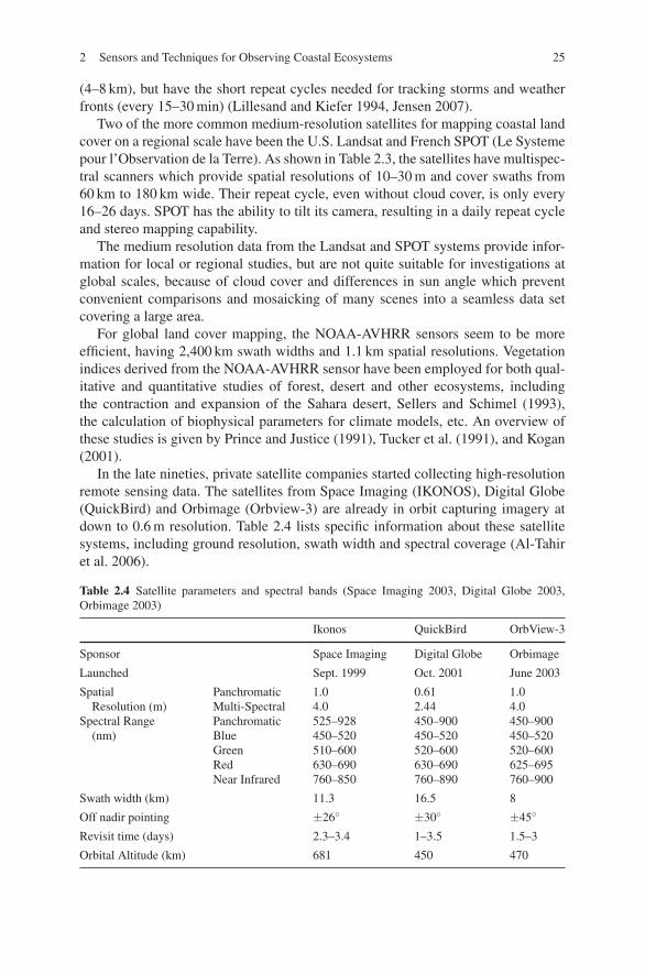
In the late nineties, private satellite companies started collecting high-resolutionremote sensing data. The satellites from Space Imaging (IKONOS), Digital Globe(QuickBird) and Orbimage (Orbview-3) are already in orbit capturing imagery atdown to 0.6 m resolution. Table 2.4 lists specific information about these satellitesystems, including ground resolution, swath width and spectral coverage (Al-Tahiret al. 2006).

Table 2.4 Satellite parameters and spectral bands (Space Imaging 2003, Digital Globe 2003,Orbimage 2003)

Ikonos QuickBird OrbView-3

Sponsor Space Imaging Digital Globe Orbimage

Launched Sept. 1999 Oct. 2001 June 2003

Spatial Panchromatic 1.0 0.61 1.0Resolution (m) Multi-Spectral 4.0 2.44 4.0

Spectral Range Panchromatic 525–928 450–900 450–900(nm) Blue 450–520 450–520 450–520

Green 510–600 520–600 520–600Red 630–690 630–690 625–695Near Infrared 760–850 760–890 760–900

Swath width (km) 11.3 16.5 8

Off nadir pointing ±26◦ ±30◦ ±45◦

Revisit time (days) 2.3–3.4 1–3.5 1.5–3

Orbital Altitude (km) 681 450 470

26 V.V. Klemas

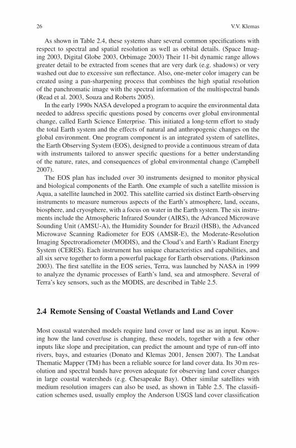
As shown in Table 2.4, these systems share several common specifications withrespect to spectral and spatial resolution as well as orbital details. (Space Imag-ing 2003, Digital Globe 2003, Orbimage 2003) Their 11-bit dynamic range allowsgreater detail to be extracted from scenes that are very dark (e.g. shadows) or verywashed out due to excessive sun reflectance. Also, one-meter color imagery can becreated using a pan-sharpening process that combines the high spatial resolutionof the panchromatic image with the spectral information of the multispectral bands(Read et al. 2003, Souza and Roberts 2005).

In the early 1990s NASA developed a program to acquire the environmental dataneeded to address specific questions posed by concerns over global environmentalchange, called Earth Science Enterprise. This initiated a long-term effort to studythe total Earth system and the effects of natural and anthropogenic changes on theglobal environment. One program component is an integrated system of satellites,the Earth Observing System (EOS), designed to provide a continuous stream of datawith instruments tailored to answer specific questions for a better understandingof the nature, rates, and consequences of global environmental change (Campbell2007).

The EOS plan has included over 30 instruments designed to monitor physicaland biological components of the Earth. One example of such a satellite mission isAqua, a satellite launched in 2002. This satellite carried six distinct Earth-observinginstruments to measure numerous aspects of the Earth’s atmosphere, land, oceans,biosphere, and cryosphere, with a focus on water in the Earth system. The six instru-ments include the Atmospheric Infrared Sounder (AIRS), the Advanced MicrowaveSounding Unit (AMSU-A), the Humidity Sounder for Brazil (HSB), the AdvancedMicrowave Scanning Radiometer for EOS (AMSR-E), the Moderate-ResolutionImaging Spectroradiometer (MODIS), and the Cloud’s and Earth’s Radiant EnergySystem (CERES). Each instrument has unique characteristics and capabilities, andall six serve together to form a powerful package for Earth observations. (Parkinson2003). The first satellite in the EOS series, Terra, was launched by NASA in 1999to analyze the dynamic processes of Earth’s land, sea and atmosphere. Several ofTerra’s key sensors, such as the MODIS, are described in Table 2.5.

2.4 Remote Sensing of Coastal Wetlands and Land Cover

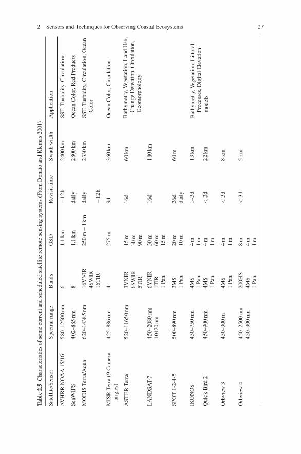
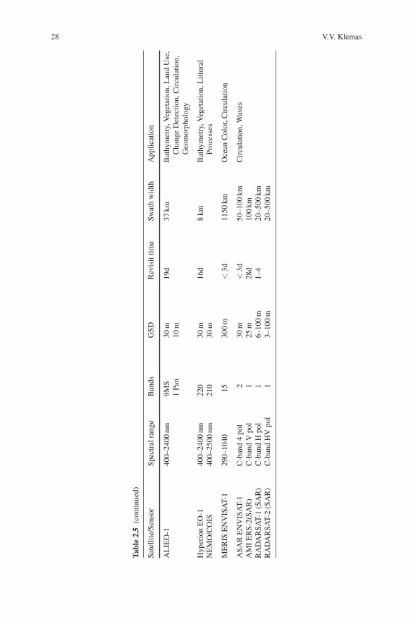
Most coastal watershed models require land cover or land use as an input. Know-ing how the land cover/use is changing, these models, together with a few otherinputs like slope and precipitation, can predict the amount and type of run-off intorivers, bays, and estuaries (Donato and Klemas 2001, Jensen 2007). The LandsatThematic Mapper (TM) has been a reliable source for land cover data. Its 30 m res-olution and spectral bands have proven adequate for observing land cover changesin large coastal watersheds (e.g. Chesapeake Bay). Other similar satellites withmedium resolution imagers can also be used, as shown in Table 2.5. The classifi-cation schemes used, usually employ the Anderson USGS land cover classification

2 Sensors and Techniques for Observing Coastal Ecosystems 27

Tabl

e2.

5C

hara

cter

istic

sof

som

ecu

rren

tand

sche

dule

dsa

telli

tere

mot

ese

nsin

gsy

stem

s(F

rom

Don

ato

and

Kle

mas

2001

)

Sate

llite

/Sen

sor

Spec

tral

rang

eB

ands

GSD

Rev

isit

time

Swat

hw

idth

App

licat

ion

AV

HR

RN

OA

A15

/16

580–

1250

0nm

61.

1km

−12

h24

00km

SST,

Tur

bidi

ty,C

ircu

latio

n

SeaW

IFS

402–

885

nm8

1.1

kmda

ily28

00km

Oce

anC

olor

,Red

Prod

ucts

MO

DIS

Terr

a/A

qua

620–

1438

5nm

16V

NIR

4SW

IR16

TIR

250

m−

1km

daily

−12

h

2330

kmSS

T,T

urbi

dity

,Cir

cula

tion,

Oce

anC

olor

MIS

RTe

rra

(9C

amer

aan

gles

)42

5–88

6nm

427

5m

9d36

0km

Oce

anC

olor

,Cir

cula

tion

AST

ER

Terr

a52

0–11

650

nm3V

NIR

6SW

IR5T

IR

15m

30m

90m

16d

60km

Bat

hym

etry

,Veg

etat

ion,

Lan

dU

se,

Cha

nge

Det

ectio

n,C

ircu

latio

n,G

eom

orph

olog

y

LA

ND

SAT-

745

0–20

80nm

6VN

IR30

m16

d18

0km

1042

0nm

1TIR

60m

1Pa

n15

m

SPO

T1-

2-4-

550

0–89

0nm

3MS

20m

26d

60m

1Pa

n10

mda

ily

IKO

NO

S45

0–75

0nm

4MS

1Pa

n4

m1

m1–

3d13

kmB

athy

met

ry,V

eget

atio

n,L

ittor

alPr

oces

ses,

Dig

italE

leva

tion

mod

els

Qui

ckB

ird

245

0–90

0nm

4MS

4m

<3d

22km

1Pa

n1

m

Orb

view

345

0–90

0m

4MS

4m

<3d

8km

1Pa

n1

m

Orb

view

445

0–25

00nm

200H

S8

m<

3d5

km45

0–90

0nm

4MS

4m

1Pa

n1

m

28 V.V. Klemas

Tabl

e2.

5(c

ontin

ued)

Sate

llite

/Sen

sor

Spec

tral

rang

eB

ands

GSD

Rev

isit

time

Swat

hw

idth

App

licat

ion

AL

IEO

-140

0–24

00nm

9MS

1Pa

n30

m10

m19

d37

kmB

athy

met

ry,V

eget

atio

n,L

and

Use

,C

hang

eD

etec

tion,

Cir

cula

tion,

Geo

mor

phol

ogy

Hyp

erio

nE

O-1

400–

2400

nm22

030

m16

d8

kmB

athy

met

ry,V

eget

atio

n,L

ittor

alPr

oces

ses

NE

MO

/CO

IS40

0–25

00nm

210

30m

ME

RIS

EN

VIS

AT-

129

0–10

4015

300

m<

3d11

50km

Oce

anC

olor

,Cir

cula

tion

ASA

RE

NV

ISA

T-1

C-b

and

4po

l2

30m

<3d

50–1

00km

Cir

cula

tion,

Wav

esA

MI

ER

S-2(

SAR

)C

-ban

dV

pol

125

m28

d10

0km

RA

DA

RSA

T-1

(SA

R)

C-b

and

Hpo

l1

6–10

0m

1–4

20–5

00km

RA

DA

RSA

T-2

(SA

R)

C-b

and

HV

pol

13–

100

m20

–500

km

2 Sensors and Techniques for Observing Coastal Ecosystems 29

system (Anderson et al. 1976) for the top level, and develop their own classifica-tion for the more detailed levels, such as the C-CAP Classification System (Klemaset al. 1993, Dobson et al. 1995). A very detailed wetlands classification system isthe one developed by Cowardin et al. (1979). However, this classification systemproved to be too complex for satellite remote sensing. Some of the ecosystem healthindicators that can be observed by remote sensors include percent of imperviousareas, natural vegetation cover, buffer degradation, wetland loss and fragmentation,wetland biomass change, invasive species, etc. (Odum 1993, Lathrop et al. 2000,Klemas 2005).

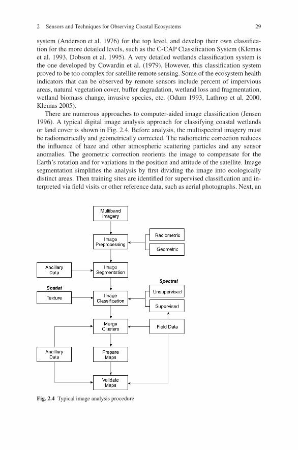
There are numerous approaches to computer-aided image classification (Jensen1996). A typical digital image analysis approach for classifying coastal wetlandsor land cover is shown in Fig. 2.4. Before analysis, the multispectral imagery mustbe radiometrically and geometrically corrected. The radiometric correction reducesthe influence of haze and other atmospheric scattering particles and any sensoranomalies. The geometric correction reorients the image to compensate for theEarth’s rotation and for variations in the position and attitude of the satellite. Imagesegmentation simplifies the analysis by first dividing the image into ecologicallydistinct areas. Then training sites are identified for supervised classification and in-terpreted via field visits or other reference data, such as aerial photographs. Next, an

Fig. 2.4 Typical image analysis procedure

30 V.V. Klemas

unsupervised classification is performed to identify variations in the image not con-tained in the training sites. Training site spectral clusters and unsupervised spectralclasses are then analyzed using cluster analysis to develop an optimum set of spec-tral signatures. Final image classification is then performed to match the classifiedthemes with the project requirements. (Lachowski et al. 1995, Jensen 1996). Textureanalysis is quite useful, but more difficult to automate and is best performed visually(Sabins 1978, Purkis 2005). Note that throughout the process, ancillary data is used,whenever available (e.g. aerial photos, maps, field data, etc.).

When studying critical wetland sites or small watersheds one can use aircraftor high resolution satellite systems. Airborne digital cameras, providing color andcolor infrared digital imagery are particularly suitable for mapping or validatingsatellite data. Such digital imagery can be integrated with GPS information and usedas georeferenced layers in a GIS for a wide range of modeling applications (Lyonand McCarthy 1995). Small aircraft flown at low altitudes (e.g. 500 m) can be usedto supplement field data. High resolution imagery (0.6–4 m) can also be obtainedfrom satellites, such as IKONOS and QuickBird (see Table 2.4). The cost becomesexcessive if the site is larger than a few hundred square kilometers. Wetland speciesidentification is difficult; however, some progress is being made using hyperspectralimagers (Schmidt et al. 2004, Porter 2006).

For looking at coastal land cover changes or beach erosion over long time pe-riods, it is important to review historical airphotos, held by local, state and federalagencies. The U.S. Geological Survey and the USDA Soil Conservation Servicehave useable aerial photos of the coast dating back to the 1930s. They also have var-ious maps, including planimetric, topographic, quadrangle, thematic, orthophoto,satellite and digital maps (Rasher and Weaver 1990, Lachowski et al. 1995). For in-stance, to map long-term changes of the shoreline due to beach erosion, time seriesof aerial photographs are used. The shoreline is divided into segments which areuniformly eroding or accreting. Then the change in the distance of the waterline ismeasured in reference to some stable feature like a coastal highway (Jensen 2007).

The actual beach profile can be obtained with low altitude LIDAR flights. Opticalwater clarity is the most limiting factor for LIDAR depth detection. Therefore, it isimportant to conduct the LIDAR overflights during tidal and current conditions thatminimize the water turbidity due to sediment resuspension and river inflow. TheLIDAR system must have a kd factor large enough to accommodate the water depthand water turbidity at the study site (k = attenuation coefficient; d = water depth).For instance, if a given LIDAR system has a kd = 3 and the turbid water has anattenuation coefficient of k = 1, the system will be effective only to depths of about3 m. Beyond that depth, one may have to use acoustic echo-sounding techniques(Brock and Sallenger 2000).

Mapping submerged aquatic vegetation (SAV) and coral reefs requires high res-olution (1–4 m) imagery (Mumby and Edwards 2002, Purkis 2005). Coral reefecosystems usually exist in clear water and can be classified to show different formsof coral reef, dead coral, coral rubble, algal cover, sand lagoons, different densitiesof seagrasses, etc. SAV may grow in more turbid waters and thus is more difficultto map. High resolution (e.g. IKONOS) multispectral imagers have been used in the

2 Sensors and Techniques for Observing Coastal Ecosystems 31

past to map SAV and coral reefs; however, hyperspectral imagers should improvethe results significantly (Maeder et al. 2002, Mishra et al. 2006).

Digital change detection using satellite imagery can be performed effectivelyby employing one of several techniques, including post-classification comparisonand temporal image differencing (Dobson et al. 1995, Jensen 1996, Lunetta andElvidge 1998). Post-classification comparison change detection requires rectifica-tion and classification of the remotely sensed images from both dates. These twomaps are then compared on a pixel-by-pixel basis. One disadvantage is that everyerror in the individual date classification maps will also be present in the final changedetection map.

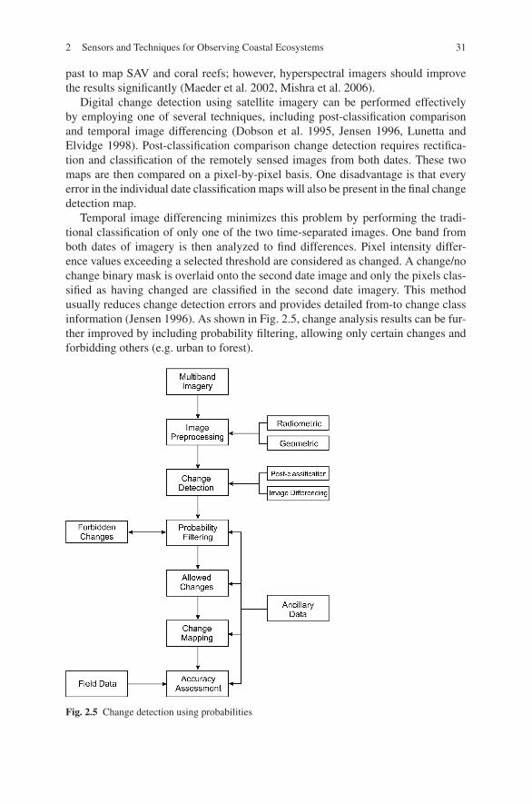
Temporal image differencing minimizes this problem by performing the tradi-tional classification of only one of the two time-separated images. One band fromboth dates of imagery is then analyzed to find differences. Pixel intensity differ-ence values exceeding a selected threshold are considered as changed. A change/nochange binary mask is overlaid onto the second date image and only the pixels clas-sified as having changed are classified in the second date imagery. This methodusually reduces change detection errors and provides detailed from-to change classinformation (Jensen 1996). As shown in Fig. 2.5, change analysis results can be fur-ther improved by including probability filtering, allowing only certain changes andforbidding others (e.g. urban to forest).

Fig. 2.5 Change detection using probabilities

32 V.V. Klemas

Biomass and vegetation indices have long been used in remote sensing for mon-itoring the health and temporal changes associated with wetland or other vegeta-tion (Goward et al. 1991, Lyon and McCarthy 1995). The spectral bands used forbiomass mapping are primarily the red band, which is absorbed by the chlorophyll inthe upper leaf layers, and a near-infrared band, which is reflected from the inner leafstructure, yet still penetrates several leaf layers and thus provides information on thecanopy thickness and density. These spectral bands are combined in the NormalizedDifference Vegetation Index (NDVI) to provide an estimate of above-ground wet-land plant biomass in grams dry weight per square meter. The NDVI consists of thedifference of the near-infrared and red band radiances (digital numbers) divided bytheir sum (Hardisky et al. 1984, Gross et al. 1987).

A particularly effective method for remotely sensing wetland changes usesbiomass as an indicator. To detect biomass changes the Modified Soil AdjustedVegetation Index (MSAVI) is used with red and near-infrared reflectances derivedfrom Landsat/TM images (Qi et al. 1994). This biomass algorithm is applied to atime series of Landsat/TM images and used with selected thresholds to detect wet-land changes. To minimize natural variations between images in the time series(e.g. atmospheric, annual, seasonal, etc.) it is assumed that the relative distributionof biomass in each sub-basin will remain essentially constant over time. Wetlandpixels whose MSAVI deviation from the sub-basin mean changes from its previousdeviation by more than a selected threshold value are considered as having changed.Threshold selection determines whether many small changes or only the more sig-nificant ones are detected. To minimize data costs, only changed sites “flagged”by Landsat/TM are studied in more detail with high-resolution systems, such asIKONOS or airborne scanners (Porter 2006, Klemas 2007).

2.5 Remote Sensing of Coastal and Estuarine Waters

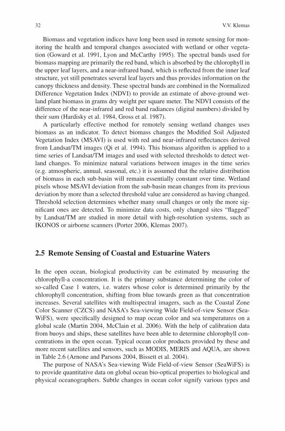
In the open ocean, biological productivity can be estimated by measuring thechlorophyll-a concentration. It is the primary substance determining the color ofso-called Case 1 waters, i.e. waters whose color is determined primarily by thechlorophyll concentration, shifting from blue towards green as that concentrationincreases. Several satellites with multispectral imagers, such as the Coastal ZoneColor Scanner (CZCS) and NASA’s Sea-viewing Wide Field-of-view Sensor (Sea-WiFS), were specifically designed to map ocean color and sea temperatures on aglobal scale (Martin 2004, McClain et al. 2006). With the help of calibration datafrom buoys and ships, these satellites have been able to determine chlorophyll con-centrations in the open ocean. Typical ocean color products provided by these andmore recent satellites and sensors, such as MODIS, MERIS and AQUA, are shownin Table 2.6 (Arnone and Parsons 2004, Bissett et al. 2004).

The purpose of NASA’s Sea-viewing Wide Field-of-view Sensor (SeaWiFS) isto provide quantitative data on global ocean bio-optical properties to biological andphysical oceanographers. Subtle changes in ocean color signify various types and

2 Sensors and Techniques for Observing Coastal Ecosystems 33

Table 2.6 Ocean color products (Arnone and Parsons 2004)

Chlorophyll concentration Biological processes such as algal (harmful andnon-harmful) blooms and decay

Spectral backscattering coefficient bb(γ) 90–180◦ particle scattering linked to concentration,composition, index of refraction of organic(marine) and inorganic (terrigenous) particles,resuspension

Spectral absorption coefficient a(λ ) Total absorption, changes in water quality

Spectral absorption colored dissolvedorganic matter a(CDOMλ )

Conservative tracer of river plumes, linked withcoastal salinity, photo-oxidation processes

Spectral particle absorption coefficienta(pλ )

Particle composition, (organic and inorganicparticles)

Spectral phytoplankton absorptioncoefficient a(φλ )

Absorption linked to differences in chlorophyllpackaging within phytoplankton cells

Remote sensing reflectance RRS(λ ) Spectral absolute water color and water signature

Diffuse attenuation coefficient(k532, k490)

Light penetration depth, light availability at depth

Aerosol concentration – Epsilon Type and distribution, affects visibility, Atmosphericcorrection methods

Beam attenuation coefficient – c(λ ) Total light attenuation using a collimated beam

Diver visibility Horizontal visibility, average target size, targetcontrast, solar overhead illumination

Laser penetration depth Underwater performance of lasers (imaging orbathymetry systems)

quantities of marine phytoplankton, the knowledge of which has many scientific andpractical applications. The ability to map the color of the world’s oceans has beenused to estimate global ocean productivity (Longhurst et al. 1995, Behrenfeld andFalkowski 1997), aid in delineating oceanic biotic provinces (Longhurst 1998), andstudy regional shelf break frontal processes (Ryan et al. 1999, Schofield et al. 2004).As shown in Table 2.5, SeaWiFS has eight spectral bands which are optimized forocean chlorophyll detection and the necessary atmospheric corrections. The spatialresolution is 1.1 km and the swath width 2,800 km. Due to the wide swath width, therevisit time is once per day. Data in the form of analyzed sea surface temperatureand chlorophyll charts are provided daily to the fisheries and shipping industriesover Marine Radio Networks. Because certain species of commercial and game fishare indigenous to waters of a specific temperature, fishermen can cut fuel costs andtime by being able to locate areas of higher catch potential (Cracknell and Hayes2007).

Wind-induced upwelling in coastal regions brings nutrients to the surface, cre-ating zones of high biological productivity, accompanied by high concentrations ofchlorophyll and phytoplankton, which can be detected by color sensors on satellites.The waters off Peru and California are good examples, where long term upwellingevents influence the abundance of fish over periods of months. When wind patternsover the Pacific Ocean change, warm waters from the Western Pacific shift to the

34 V.V. Klemas

Eastern Pacific and the upwelling of nutrient-rich cold water off the Peruvian coastis suppressed, resulting in well-recognized “El Nino” conditions (Yan et al. 1993).Such upwelling areas and their condition can be observed by satellites with thermalinfrared imagers, such as NOAA’s AVHRR, or ocean color sensors, such as Sea-WiFS (Schofield et al. 2004, Martin 2004).

As one approaches the coast and enters the bays and estuaries, the water be-comes quite turbid and contains suspended sediment, dissolved organics and othersubstances, in addition to chlorophyll. To identify each substance in this complexmixture of Case 2 waters requires hyperspectral sensors and more sophisticated al-gorithms than the empirical regression models (Sydor 2006, Cannizzaro and Carder2006) used in Case 1 waters in the open ocean (Ikeda and Dobson 1995, Bukata2005). Neural network approaches have been used to map chlorophyll and sus-pended sediment concentrations in Delaware Bay and other estuaries (Keiner andBrown 1999, Dzwonkowski and Yan 2005a). Neural networks, however, require ex-tensive calibration with coincident ship and satellite observations of radiance, andshipboard measurements of chlorophyll and sediment concentrations.

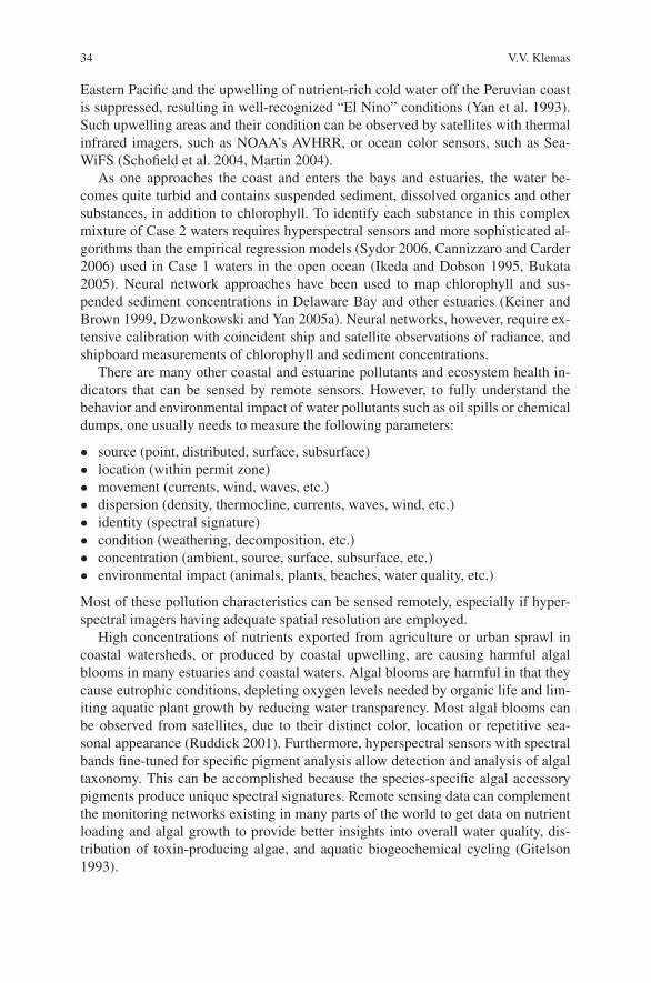
There are many other coastal and estuarine pollutants and ecosystem health in-dicators that can be sensed by remote sensors. However, to fully understand thebehavior and environmental impact of water pollutants such as oil spills or chemicaldumps, one usually needs to measure the following parameters:

• source (point, distributed, surface, subsurface)• location (within permit zone)• movement (currents, wind, waves, etc.)• dispersion (density, thermocline, currents, waves, wind, etc.)• identity (spectral signature)• condition (weathering, decomposition, etc.)• concentration (ambient, source, surface, subsurface, etc.)• environmental impact (animals, plants, beaches, water quality, etc.)

Most of these pollution characteristics can be sensed remotely, especially if hyper-spectral imagers having adequate spatial resolution are employed.

High concentrations of nutrients exported from agriculture or urban sprawl incoastal watersheds, or produced by coastal upwelling, are causing harmful algalblooms in many estuaries and coastal waters. Algal blooms are harmful in that theycause eutrophic conditions, depleting oxygen levels needed by organic life and lim-iting aquatic plant growth by reducing water transparency. Most algal blooms canbe observed from satellites, due to their distinct color, location or repetitive sea-sonal appearance (Ruddick 2001). Furthermore, hyperspectral sensors with spectralbands fine-tuned for specific pigment analysis allow detection and analysis of algaltaxonomy. This can be accomplished because the species-specific algal accessorypigments produce unique spectral signatures. Remote sensing data can complementthe monitoring networks existing in many parts of the world to get data on nutrientloading and algal growth to provide better insights into overall water quality, dis-tribution of toxin-producing algae, and aquatic biogeochemical cycling (Gitelson1993).

2 Sensors and Techniques for Observing Coastal Ecosystems 35

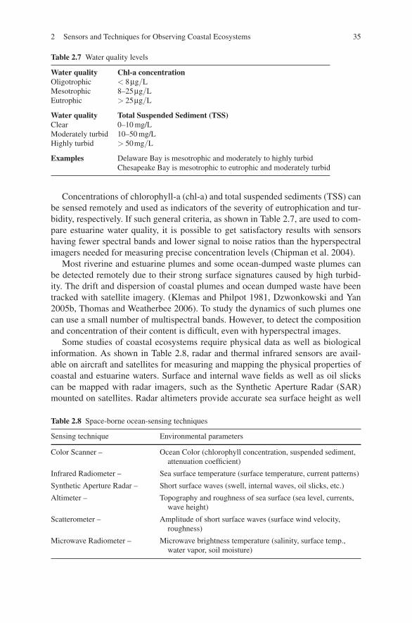
Table 2.7 Water quality levels

Water quality Chl-a concentrationOligotrophic < 8μg/LMesotrophic 8–25μg/LEutrophic > 25μg/L

Water quality Total Suspended Sediment (TSS)Clear 0–10 mg/LModerately turbid 10–50 mg/LHighly turbid > 50mg/L

Examples Delaware Bay is mesotrophic and moderately to highly turbidChesapeake Bay is mesotrophic to eutrophic and moderately turbid

Concentrations of chlorophyll-a (chl-a) and total suspended sediments (TSS) canbe sensed remotely and used as indicators of the severity of eutrophication and tur-bidity, respectively. If such general criteria, as shown in Table 2.7, are used to com-pare estuarine water quality, it is possible to get satisfactory results with sensorshaving fewer spectral bands and lower signal to noise ratios than the hyperspectralimagers needed for measuring precise concentration levels (Chipman et al. 2004).

Most riverine and estuarine plumes and some ocean-dumped waste plumes canbe detected remotely due to their strong surface signatures caused by high turbid-ity. The drift and dispersion of coastal plumes and ocean dumped waste have beentracked with satellite imagery. (Klemas and Philpot 1981, Dzwonkowski and Yan2005b, Thomas and Weatherbee 2006). To study the dynamics of such plumes onecan use a small number of multispectral bands. However, to detect the compositionand concentration of their content is difficult, even with hyperspectral images.

Some studies of coastal ecosystems require physical data as well as biologicalinformation. As shown in Table 2.8, radar and thermal infrared sensors are avail-able on aircraft and satellites for measuring and mapping the physical properties ofcoastal and estuarine waters. Surface and internal wave fields as well as oil slickscan be mapped with radar imagers, such as the Synthetic Aperture Radar (SAR)mounted on satellites. Radar altimeters provide accurate sea surface height as well

Table 2.8 Space-borne ocean-sensing techniques

Sensing technique Environmental parameters

Color Scanner – Ocean Color (chlorophyll concentration, suspended sediment,attenuation coefficient)

Infrared Radiometer – Sea surface temperature (surface temperature, current patterns)

Synthetic Aperture Radar – Short surface waves (swell, internal waves, oil slicks, etc.)

Altimeter – Topography and roughness of sea surface (sea level, currents,wave height)

Scatterometer – Amplitude of short surface waves (surface wind velocity,roughness)

Microwave Radiometer – Microwave brightness temperature (salinity, surface temp.,water vapor, soil moisture)

36 V.V. Klemas

as wave amplitude information. Radar scatterometer data can be analyzed to extractsea surface winds. (Martin 2004, Elachi and van Ziel 2006). The two passive de-vices, microwave radiometers and thermal infrared scanners can sense sea surfacesalinity and temperature, respectively. Microwave radiometers can also measure awide range of climate related parameters, such as soil moisture (Parkinson 2003,Burrage et al. 2003).

Oil spills are best detected by imaging radars, such as SAR on satellites, becauseoil slicks dampen small surface wavelets, which otherwise backscatter a strong radarreturn signal. Small aircraft can be used to verify oil spill drift and dispersion mod-els by tracking the movement and spreading of oil slicks in coastal waters and theirinteractions with fronts. A typical estuarine front may be caused by flooding higherdensity ocean water gliding under the lower density, lower salinity river water andthus causing a strong convergence zone, which may be marked by a foam line andcolor line. Estuarine fronts are narrow features, quite dynamic and have high con-vergence velocities (Sarabun 1993). Coastal and estuarine fronts can concentratenutrients, pollutants and capture oil slicks causing their paths to deviate from driftand dispersion model predictions (Klemas 1980). To study frontal dynamics andtrack oil slicks one needs spatial and temporal resolutions of 10–50 m and 0.5–3 h,respectively.

Currents and breaking waves strongly affect coastal ecosystems, especially in thenearshore, which is an extremely dynamic environment. Currents influence the driftand dispersion of various pollutants, and together with breaking waves mobilizeand transport sediments, resulting in erosion and morphological evolution of naturalbeaches. Changes in the underlying bathymetry in turn affect the wave and currentpatterns, resulting in a feedback mechanism between the hydrodynamics and mor-phology. The ability to monitor these processes is necessary in order to understandand predict the changes that occur in the nearshore region. Arrays of current meters,acoustic Doppler velocimeters, and pressure sensors are not very effective for de-termining surface currents and waves over large coastal regions, since these sensorsmeasure currents at a point and are expensive, when large numbers of sensors haveto be deployed.

Shore-based high frequency (HF) and microwave Doppler radar systems are usedto map currents and determine swell-wave parameters in coastal waters with con-siderable accuracy. (Paduan and Graber 1997, Graber et al. 1997, Bathgate et al.2006). The surface current measurements use the concept of Bragg scattering froma slightly rough sea surface, modulated by Doppler velocities of the surface cur-rents. Extraction of swell direction, height and period from HF radar data is basedon the modulation imposed on the short Bragg wavelets by the longer faster movingswell. HF radars can determine coastal currents and wave conditions over a rangeof up to 200 km. (Cracknell and Hayes 2007). While HF radar provides accuratemaps of surface currents and wave information for large coastal areas, their spatialresolution, which is about 1 km, is more suitable for measuring mesoscale featuresthan small scale currents. On the other hand, shore-based microwave X-band andS-band radars have resolutions of the order of 10 m, yet have a range of only a fewkilometers.

2 Sensors and Techniques for Observing Coastal Ecosystems 37

Estimates of currents over large coastal areas, such as the continental shelf, canalso be obtained by tracking the movement of drogues, dyes or natural surface fea-tures which differ detectably in color or temperature from the background waters(Davis 1985, Breaker et al. 1994). Examples of such features include sediment orchlorophyll plumes, patches of different water temperature, surface slicks, coastalfronts, etc.

Large ocean internal waves on continental shelves strongly influence acousticwave propagation; submarine navigation; mixing nutrients to euphotic zone; sed-iment resuspension; cross-shore pollutant transport; and coastal engineering andoil exploration. Internal waves move along pycnoclines, which are surfaces thatseparate water masses of different densities. The water column is frequently nothomogeneous, but stratified, containing thermoclines and pycnoclines that markboundaries between water masses. The periods of internal waves are measured inminutes, rather than in seconds, and their wavelengths in kilometers rather than intens of meters. Furthermore, the larger internal waves can attain heights of 100 m(Alford 2003). The period of the internal wave packets approximates the periodof the tides, suggesting a cause-and-effect relationship. Internal waves can be de-tected visually and by radar since they cause local currents which modulate surfacewavelets and slicks (Zhao et al. 2004).

Oil tankers, cargo ships, pleasure craft and military vessels navigating in bayssuch as Delaware Bay or Chesapeake Bay and further north, require informationon the extent and type of ice cover during winter months. Types of ice cover mayinclude fast ice, pack ice, large drift ice, small drift ice, etc. Radar and multispectralvisible bands can provide such information.

The devastating effects of Atlantic hurricanes and tsunamis in the Indian Oceanbring out the need for timely monitoring of coastal flooding. There are many otherstorm events, such as Nor’easters, that impact the Atlantic coast more frequentlythan hurricanes. A good example of a major coastal flooding event is the Nor’easterstorm of 1962 (Mather et al. 1967). The waves and storm surge broke through thedune line, flooded the entire coastal zone and damaged boardwalks and homes insettlements along the mid-Atlantic coast. The extensive damage and flooding alongthe coast was captured in aerial photographs after the storm.

Obtaining images before and after the landfall of hurricane Katrina in NewOrleans in 2005, Landsat TM effectively showed the wetland losses and inunda-tion over the entire region at 30 m resolution, while high resolution satellites, likeIKONOS and QuickBird, documented the details, including actual breaks in thelevees protecting the city. However, more frequent repeat cycles would have beenuseful for emergency operations. Only SAR could penetrate the clouds to observecoastal inundation conditions during the time of the hurricane’s landfall. Radar candetect flooded coastal marshes because they usually provide a weaker radar returnthan non-flooded ones. The marsh grasses may calm the water surface accentuatingspecular reflection (Ramsey 1995). The radar return from flooded forests is usuallyenhanced compared to returns from nonflooded forests. The enhancement is due tothe double bounce mechanism where the signal penetrating the canopy is reflectedoff the water surface and subsequently reflected back toward the sensor by a secondreflection off a tree trunk (Hess et al. 1990).

38 V.V. Klemas

2.6 Field Data

Field or ship data need to be collected for developing a spectral “signature library”for supervised classification of land cover, calibrating remotely sensed data or train-ing neural networks. Field checks may also have to be conducted in order to guidethe interpreters during the image classification stage. Finally, field data is gatheredat the end of a project to validate the remotely sensed products (e.g. wetland maps)and assess their accuracy.

Training sites for supervised classification of coastal land cover must meet well-defined criteria. They should be homogeneous with regard to vegetation/land coverand in accessible areas. They should be large enough so they can be located onsatellite images, but small enough to minimize within-site variation (10–25 pixelsin size). Multiple training sites for each category of the classification scheme arerequired. (e.g. 10 sites).

To determine the reflectance characteristics of a land surface, a goniometer can beused to measure the Bidirectional Reflectance Distribution Function (BRDF). Thisis a tedious procedure, requiring that the irradiance and radiance be measured at allsensor positions and all solar angles. A more practical way is to compare the site’sreflectance with that of a Lambertian white panel (diffuse reflector) made of specialmaterials, such as Halon, having controlled reflectivities from 95% to 99% (McCoy2005, Jensen 2007). To convert ground reflectances to at-satellite-reflectances, onecan use large white canvas sheets or natural targets large enough to be identifiablein the satellite imagery and having reflectances covering the entire range of thereflectances of the land cover sites to be mapped. (e.g. a corn field, a large lawn, afield of dry soil, etc.). By measuring the reflectances of these targets on the groundand at the satellite, and comparing them with the Lambertian white (Halon) panels,one can calibrate the satellite sensor so it could measure the reflectances of all thepixels in the scene (Gross et al. 1987).

To validate the remote sensing results and determine their accuracy, a statisti-cally valid sampling scheme should be selected. For instance, for land cover maps asystematic unaligned sampling pattern is frequently used. On the other hand, somesituations may require a clustered or stratified random sampling pattern. Tests byvarious researchers have shown the simple random and stratified random patternsboth give satisfactory results. However, the stratified random approach requiressome advance knowledge of where the land cover boundaries are located (McCoy2005).

The accuracy of completed map products can be expressed in terms of an errormatrix for land cover mapping applications and as percentage error for water qualitystudies. Furthermore, a Kappa coefficient can be calculated to show how much betterthe map results are than a totally random labeling of the pixels in the image (Jensen1996, Campbell 2007).

Instrumented ships, buoys, and ocean gliders are used to calibrate and validatechlorophyll-a and total suspended sediment maps obtained with multispectral oceancolor sensors. Some typical ship or buoy measurements are shown in Table 2.9. Incoastal and estuarine waters this data must frequently be obtained very close to the

2 Sensors and Techniques for Observing Coastal Ecosystems 39

Table 2.9 Remote sensing related ship measurements

Direct measurementsTemperature, Salinity, Secchi Depth, pH, Attenuation Coefficient, Spectral Reflectance

(Radiance and Irradiance)

Water sample analysisChl-a, TSS, Nitrogen, Phosphorus

Ship data acquisitionWater samples obtained from upper 0.5 m of water column; Ship data obtained within 20 min of

satellite overpass; GPS used for sample site location

satellite overpass time and be statistically representative of prevailing conditions.The water samples are usually taken from the upper half meter of the water column.Sites for calibrating remotely sensed data, such as chlorophyll concentrations incoastal waters, must be located at well-known points representing the entire rangeof variables to be measured.

2.7 Summary and Conclusions

Since the early 1970s, civilian remote sensing satellites have made major contri-butions to our understanding of the Earth’s ecosystems and warned us of criticalnatural and man-made changes taking place, such as deforestation, desertificationand shrinking glaciers in Greenland and the Antarctic. In the open ocean, satelliteshave tracked storms and major oil spills. They have also monitored fisheries-relatedchlorophyll concentrations, algal blooms and sea surface temperatures. However,obtaining this information for coastal and estuarine ecosystems is more challeng-ing, since they exhibit extreme variations in spatial complexity and temporal vari-ability. After several decades of improvements, it now appears that remote sensingneeds, cost and technology are converging in a way that will prove practical andcost-effective for coastal managers and ecosystem researchers. A few specific con-clusions and recommendations are outlined below:

• As shown in Table 2.2, remote sensing of coastal ecosystems requires high spa-tial, spectral, and temporal resolution.

• Aerial photography of coastal ecosystems is usually performed at medium al-titudes with color film, color infrared film and digital cameras at scales of1:1,200–1:24,000. Large coastal regions can be mapped from high altitudes(scale 1:100,000), while low altitude flights (scale 1:600) can be used in supportof field data collection (Jensen 2007, Campbell 2007).

• Georeferenced orthophotos, topographic maps and land cover maps representgood base maps for creating a multi-layer GIS database. Digital camera imagesare especially suited for use with GIS databases and for interpreting land covermaps derived from satellite imagery (Porter 2006).

40 V.V. Klemas

• To keep costs reasonable, large coastal watersheds should be studied with mediumresolution satellite sensors (e.g. 30 m Landsat TM) and only small areas and crit-ical sites mapped with airborne or high resolution satellite sensors (e.g. 1–4 mIKONOS).

• For detecting changes of coastal land cover, including tidal marshes, in a time-series of images, post-classification comparison, image differencing and biomasschange techniques can be used. To determine man-made changes, the imagesmust be corrected for natural variations such as atmospheric, inter-annual, sea-sonal, and tidal differences (Lunetta and Elvidge 1998).

• On land, field data are often collected along transects using systematic randomsampling. The sampling scheme should be optimized for each type of imageclassification approach, e.g. supervised, unsupervised, etc. (McCoy 2005, Jensen1996).

• Mapping wetlands, coral reefs and submerged aquatic vegetation requires highresolution (1–4 m) imagery. Wetland species identification is possible only withhyperspectral sensors and large amounts of field data (Klemas 2005, Mumby andEdwards 2002, Schmidt et al. 2004).

• Airborne LIDAR is effective for near-shore bathymetry, but in turbid waterswhen the kd product exceeds the vendor specified value, acoustic echo sound-ing techniques must be used (k = attenuation coefficient; d = depth) (Brock andSallenger 2000).

• Coastal and estuarine waters contain a complex mixture of chlorophyll, sus-pended sediments, dissolved organics, and other substances. Therefore, hyper-spectral imagers, calibrated ship data and advanced algorithms or neural networkmethods are required to map the concentrations of these substances (Ikeda andDobson 1995).

• Approximate concentrations of chl-a and total suspended sediments can be ob-tained with multispectral scanners and a small number of ship samples.

• Ship samples and water reflectances must be gathered very close to satellite over-pass times. Spotter planes can be used to guide the research vessels to waterfeatures of interest.

• Thermal infrared radiometers or imagers, such as the AVHRR on NOAA satel-lites, can map sea surface temperature to within 0.5◦C accuracy.

• Radar altimeters, scatterometers and SAR imagers can be used for mapping sealevel height, sea surface winds, waves and currents (Ikeda and Dobson 1995,Martin 2004).

References

Alford MH (2003) Redistribution of energy available for ocean mixing by long-range propagationof internal waves. Nature 423:159–162

Al-Tahir A, Baban SMJ, Ramlal B (2006) Utilizing emerging geo-imaging technologies for themanagement of tropical coastal environments. West Indian J Eng 29:11–22

2 Sensors and Techniques for Observing Coastal Ecosystems 41

Anderson JR, Hardy EE, Roach JT, Witmer RE (1976) A land use and land cover classifica-tion system for use with remote sensor data. US Geological Survey Professional Paper 964,Washington, DC, 28p

Arnone RA, Parsons AR (2004) Real-time use of ocean color remote sensing for coastal monitor-ing. In: Miller RL, Del Castillo CE, McKee BA (eds) Remote sensing of the coastal environ-ment. Springer Publishing, Kluwer Academic, New York

Avery TE, Berlin GL (1992) Fundamentals of remote sensing and airphoto interpretation.Macmillan, New York

Bathgate J, Heron M, Prytz A (2006) A method of swell parameter extraction from HF oceansurface radar spectra. IEEE J Oceanic Eng 31:812–818

Behrenfeld MJ, Falkowski PG (1997) Photosynthetic rates derived from satellite-based chlorophyllconcentration. Limnol Oceanogr 42:1–20

Bissett WP, Arnone R, Davis CO, Dye D, Kohler DDR, Gould R (2004) From meters to kilometers-a look at ocean color scales of variability, spatial coherence, and the need for fine scale remotesensing in coastal ocean optics. Oceanography 17:32–43

Breaker LC, Krasnopolski VM, Rao DB, Yan X-H (1994) The feasibility of estimating ocean sur-face currents on an operational basis using satellite feature tracking methods. Bull Am MeteorSoc 75:2085–2095

Brock J, Sallenger A (2000) Airborne topographic LIDAR mapping for coastal science. U.S. Geo-logical Survey, Open-File Report 01–46

Bukata R (2005) Satellite monitoring of inland and coastal water quality: retrospection, introspec-tion, future directions. Taylor & Francis, London

Burrage DM, Heron ML, Hacker JM, Miller JL, Stieglitz TC, Steinberg CR, Prytz A (2003) Struc-ture and influence of tropical river plumes in the Great Barrier reef: Application and perfor-mance of an airborne sea surface salinity mapping system. Remote Sens Envir 85:204–220

Campbell JB (2007) Introduction to remote sensing. The Guilford Press, New YorkCannizzaro JP, Carder KL (2006) Estimating chlorophyll-a concentrations from remote sensing

reflectance in optically shallow waters. Remote Sens Envir 101:13–24Chipman JW, Lillesand TM, Schmaltz JE, Leale JE, Nordheim MJ (2004). Mapping lake water

clarity with Landsat images in Wisconsin, USA. Can J Remote Sens 30:1–7Cowardin L, Carter V, Golet F, LaRoe E (1979) Classification of wetlands and deep water habi-

tats of the United States. US Department of the Interior, Fish and Wildlife Service, Office ofBiological Services, FWS/OBS-79/31. Washington, DC, 131p

Cracknell AP, Hayes L (2007) Introduction to remote sensing. CRC Press, New YorkDavis RE (1985) Drifter observations of coastal surface currents during CODE: the method and

descriptive view. J Geophys Res 90:4741–4755Digital Globe (2003) Quickbird imagery products and product guide (revision 4). Digital Globe,

Inc., Colorado, USADobson JE, Bright EA, Ferguson RL, Field DW, Wood LL, Haddad KD, Iredale H, Jensen JR,

Klemas V, Orth RJ, Thomas JP (1995) NOAA Coastal Change Analysis Program (C-CAP):Guidance for regional implementation, NOAA Technical Report NMFS 123, U.S. Departmentof Commerce, Washington, DC

Donato T, Klemas V (2001) Remote sensing and modeling applications for coastal resource man-agement. Geocarto Int 16:23–29

Dzwonkowski B, Yan X-H (2005a) Development and application of a neural network based oceancolor algorithm in coastal water. Int J Remote Sens 26:1175–1200

Dzwonkowski B, Yan X-H (2005b) Tracking of a Chesapeake Bay estuarine outflow plume withsatellite-based ocean color data. Continental Shelf Res 25:1942–1958

Elachi C, van Ziel J (2006) Introduction to the physics and techniques of remote sensing. JohnWiley & Sons, New Jersey

Gitelson A (1993) Quantitative remote sensing methods for real-time monitoring of inland waterquality. Int J Remote Sens 14:1269–1295

Goward SN, Markham B, Dye DG, Dulaney W, Yang J (1991) Normalized Difference VegetationIndex measurements from the Advanced Very High Resolution Radiometer. Remote Sens Envir35:257–277

42 V.V. Klemas

Graber H, Haus B, Chapman R, Shay L (1997) HF radar comparisons with moored estimatesof current speed and direction: expected differences and implications. J Geophys Res 102:18,749–18, 766

Gross MF, Hardisky MA, Klemas V, Wolf PL (1987) Quantification of biomass of the marsh grassSpartina Alterniflora Loisel using Landsat Thematic Mapper imagery. Photogramm Eng Re-mote Sens 53:1577–1583

Hardisky MA, Daiber FC, Roman CT, Klemas V (1984) Remote sensing of biomass and annualnet aerial productivity of a salt marsh. Remote Sens Envir 16:91–106

Hess L, Melack J, Simonett D (1990) Radar detection of flooding beneath the forest canopy: areview. Int J Remote Sens 11:1313–1325

Ikeda M, Dobson FW (1995) Oceanographic applications of remote sensing. CRC Press, New YorkJensen JR (1996) Introductory digital image processing: a remote sensing perspective.

Prentice-Hall, New JerseyJensen JR (2007) Remote sensing of the environment: an Earth resource perspective. Prentice Hall,

New JerseyKeiner LE, Brown CW (1999) Estimating oceanic chlorophyll concentrations with neural net-

works. Int J Remote Sens 20:189–194Kerr JT, Ostrovsky M (2003) From space to species: ecological applications of remote sensing.

Trends Ecol Evol 18:299–305Klemas V (1980) Remote sensing of coastal fronts and their effects on oil dispersion. Int J Remote

Sens 1:11–28Klemas V (2005) Remote sensing: Wetlands classification. In: Schwartz ML (ed) Encyclopedia of

coastal science. Springer, Dordrecht, The Netherlands, pp 804–807Klemas V (2007) Remote sensing of coastal wetlands and estuaries. Proc of Coastal Zone 07.

NOAA Coastal Services Center, Charleston, South CarolinaKlemas V, Dobson JE, Ferguson RL, Haddad KD (1993) A coastal land cover classification system

for the NOAA Coastwatch Change Analysis Project. J Coast Res 9:862–872Klemas V, Philpot W (1981) Drift and dispersion studies of ocean-dumped waste using Landsat

imagery and current drogues. Photogram Eng Remote Sens 47:533–542Kogan FN (2001) Operational space technology for global vegetation assessment. Bull Amer Me-

teor Soc 82:1949–1964Lachowski H, Maus P, Golden M, Johnson J, Landrum V, Powell J, Varner V, Wirth T, Gonza-

les J, Bain S (1995) Guidelines for the use of digital imagery for vegetation mapping. U.S.Department of Agriculture, Forest Service EM-7140-25, Washington, DC

Lathrop RG, Cole MB, Showalter RD (2000) Quantifying the habitat structure and spatial patternof New Jersey (USA) salt marshes under different management regimes. Wetl Ecol Manag8:163–172

Leica (2002) ADS40 Airborne digital sensor. Leica Geosystems, GIS and Mapping, LLC, Atlanta,Georgia, USA

Lillesand TM, Kiefer RW (1994) Remote sensing and image interpretation. John Wiley & Sons,New Jersey

Longhurst A (1998) Ecological Geography of the Sea. Academic Press, LondonLonghurst A, Sathyendranath S, Platt T, Caverhill C (1995) An estimate of global primary produc-

tion in the ocean from satellite data. J Plank Res 17:1245–1271Lunetta RS, Elvidge CD (1998) Remote sensing change detection: environmental monitoring

methods and applications. Ann Arbor Press, MichiganLyon JG, McCarthy J (1995) Wetland and environmental applications of GIS. Lewis Publishers,

New YorkMaeder J, Narumalani S, Rundquist D, Perk R, Schalles J, Hutchins K, Keck J (2002) Classify-

ing and mapping general coral reef structure using Ikonos data. Photogram Eng Remote Sens68:1297–1305

Martin S (2004) An introduction to remote sensing. Cambridge University Press, CambridgeMather JR, Field RT, Yoshioka GA (1967) Storm damage hazard along the East Coast of the United

States. J Appl Meteor 6:20–30

2 Sensors and Techniques for Observing Coastal Ecosystems 43

McClain C, Hooker S, Feldman G, Bontempi P (2006) Satellite data for ocean biology, biogeo-chemistry, and climate research. Eos, Transactions, Amer Geophys Union 87:337–343

McCoy R (2005) Field methods in remote sensing. Guilford Press, New YorkMishra D, Narumalani S, Rundquist D, Lawson M (2006) Benthic habitat mapping in tropi-

cal marine environments using QuickBird multispectral data. Photogram Eng Remote Sens72:1037–1048

Mumby PJ, Edwards AJ (2002) Mapping marine environments with Ikonos imagery: enhancedspatial resolution can deliver greater thematic accuracy. Remote Sens Envir 82:248–257

Odum EP (1993) Ecology and Our Endangered Life-Support Systems, 2nd edn. Sinauer Asso-ciates, Inc., Sunderland, MA

Orbimage (2003) OrbView-3 Satellite and ground systems specifications. Orbimage Inc., Vir-ginia, USA

Paduan JD, Graber HC (1997) Introduction to high-frequency radar: Reality and myth. Oceanog-raphy 10:36–39

Parkinson CL (2003) Aqua: An earth-observing satellite mission to examine water and other cli-mate variables. IEEE T Geosci and Remote 41:173–183

Porter DE (2006) RESAAP/Final Report, NOAA/NERRS Remote sensing applications assessmentproject. University of South Carolina

Prince SD, Justice CO (1991) Coarse resolution remote sensing of the Sahelian environment. Int JRemote Sens 12:1133–1421

Purkis SJ (2005) A reef-up approach to classifying coral habitats from IKONOS imagery. IEEE TGeosci Remote 43:1375–1390

Qi J, Chehbouni A, Huete AR, Kerr YH, Sorooshian S (1994) A modified soil adjusted vegetationindex. Remote Sens Envir 48:119–126

Ramsey E (1995) Monitoring flooding in coastal wetlands by using radar imagery and ground-based measurements. Int J Remote Sens 16:2495–2502

Rasher ME, Weaver W (1990) Basic photo interpretation: a comprehensive approach to interpreta-tion of vertical aerial photography for natural resource applications. U.S. Department of Agri-culture, Washington, DC

Read JM, Clark DB, Venticinque EM, Moreira MP (2003) Application of merged 1-m and 4-mresolution satellite data to research and management in tropical forests. J Appl Ecol 40:592–600

Ruddick KG (2001) Optical remote sensing of chlorophyll-a in case 2 waters by use of an adaptivetwo-band algorithm with optimal error properties. Appl Optics 40:3575–3585

Ryan JP, Yoder JA, Cornillon PC, Barth JA (1999) Chlorophyll enhancement and mixing associ-ated with meanders of the shelf break front in the Mid-Atlantic Bight. J Geophys Res 104:23,479–23, 493

Sabins FF (1978) Remote sensing: principles and interpretation, 2nd edn. Freeman & Co,New York

Sarabun CC (1993) Observations of a Chesapeake Bay tidal front. Estuaries 16:68–73Schmidt KS, Skidmore AK, Kloosterman EH, Van Oosten H, Kumar L, Janssen JAM (2004) Map-

ping coastal vegetation using an expert system and hyperspectral imagery. Photogram Eng Re-mote Sens 70:703–716

Schofield O, Arnone RA, Bissett WP, Dickey TD, Davis CO, Finkel Z, Oliver M, Moline MA(2004) Watercolors in the Coastal Zone: What can we see? Oceanography 17:25–31

Sellers PJ, Schimel D (1993) Remote sensing of the land biosphere and biochemistry in the EOSera: science priorities, methods of implementation – EOS biosphere and biochemical panels.Global Planet Change 7:279–297

Souza CM, Roberts DA (2005) Mapping forest degradation in the Amazon region with Ikonosimages. Int J Remote Sens 26:425–429

Space Imaging (2003) IKONOS Imagery products and product guide (version 1.3). Space ImagingLLC., Colorado, USA

Sydor M (2006) Use of hyperspectral remote sensing reflectance in extracting the spectral volumeabsorption coefficient for phytoplankton in coastal water: remote sensing relationships for theinherent optical properties of coastal water. J Coastal Res 22:587–594

44 V.V. Klemas

Thomas AC, Weatherbee RA (2006) Satellite-measured temporal variability of the Columbia Riverplume. Remote Sens Envir 100:167–178

Tucker CJ, Dregne HE, Newcomb WW (1991) Expansion and contraction of the Saharan desertfrom 1980 to 1990. Science 253:299–301

Yan X-H, Ho C, Zheng Q, Klemas V (1993) Using satellite IR in studies of the variabilities of theWestern Pacific Warm Pool. Science 262:440–441

Zhao X, Klemas V, Zheng Q, Li X, Yan X-H (2004) Estimating parameters of a two-layer stratifiedocean from polarity conversion of internal solarity waves observed in satellite SAR images.Remote Sens Envir 94:276–287